Embed Size (px)
Citation preview

–조시 윌스(Josh Wills)
데이터 과학자(명사) : ’어떠한 소프트웨어공학자보다 통계학을 잘 알고 어떠한 통계학자보다 소프트웨어
공학을 잘 아는 사람’

알고리즘이란?
• 어떤 과업을 달성하기 위한 단계 / 법칙을 모은 절차
• 대용량의 데이터를 다룰 때 효율성 / 계산시간 측면에서 가장 좋아야 함
• 데이터 과학 알고리즘의 종류
• 데이터 변환, 사전준비, 처리 알고리즘
• 모수추정을 위한 최적화 알고리즘
• 기계학습 알고리즘

기계학습 알고리즘
• 예측, 분류, 군집화에 사용
• 통계학 v.s. 컴퓨터과학
• 컴퓨터과학: 가장 정확하게 예측/분류 목적 (상품화)
• 통계학: 내재되어있는 생성과정 추론 목적 (모형화)
• 데이터 과학자는 두 접근방법 사이에서 균형/가치 발견

통계학 컴퓨터공학
모수의 해석 각 모수의 현실세계 의미 탐구
모수 해석보다 예측력 최적화에 관심
신뢰구간불확실성 도출
(신뢰구간, 사후확률, 모수의 변동성 등)
신뢰구간, 불확실성을 따지지 않음
명시적 가정 가정을 명시적으로 밝히고 모수 추정 가정이 없거나 숨겨짐

세 가지 기본 알고리즘
• 데이터로 해결 가능한 현실 문제 => 분류와 예측 문제
• 문제에 어떤 해법을 사용해야 하나?
• 문제의 내용과 속성을 이해
• 어떤 알고리즘을 적용할 지 고민
• 알고리즘을 어떻게 적용할 것 인지 고민
• 기계로 자동화 해서 어떤 패턴을 보고자 하는가?

선형회귀 (Linear Regression)
• 두 개의 변수 간에 수학적인 관계 분석
• 하나의 변수와 다른 여러 변수 간에 선형관계가 있다고 가정
• 변수를 통한 미래결과 예측, 상황 파악을 위한 관계이해에 사용
• 추세와 변이를 모형화 함

선형회귀 - 모형 탐색
number of users several days or weeks in advance. But for now, youare simply trying to build intuition and understand your dataset.
You eyeball the first few rows and see:
7 276
3 43
4 82
6 136
10 417
9 269
Now, your brain can’t figure out what’s going on by just looking at them(and your friend’s brain probably can’t, either). They’re in no obviousparticular order, and there are a lot of them. So you try to plot it as inFigure 3-2.
Figure 3-2. Looking kind of linear
Three Basic Algorithms | 59
www.it-ebooks.info
It looks like there’s kind of a linear relationship here, and it makes sense;the more new friends you have, the more time you might spend on thesite. But how can you figure out how to describe that relationship?Let’s also point out that there is no perfectly deterministic relationshipbetween number of new friends and time spent on the site, but it makessense that there is an association between these two variables.Start by writing something downThere are two things you want to capture in the model. The first is thetrend and the second is the variation. We’ll start first with the trend.
First, let’s start by assuming there actually is a relationship and that it’slinear. It’s the best you can do at this point.
There are many lines that look more or less like they might work, asshown in Figure 3-3.
Figure 3-3. Which line is the best fit?
60 | Chapter 3: Algorithms
www.it-ebooks.info
모형을 찾는다:
So how do you pick which one?
Because you’re assuming a linear relationship, start your model byassuming the functional form to be:
y = β0 + β1x
Now your job is to find the best choices for β0 and β1 using the ob‐served data to estimate them: x1, y1 , x2, y2 , . . . xn, yn .
Writing this with matrix notation results in this:
y = x · β
There you go: you’ve written down your model. Now the rest is fittingthe model.Fitting the modelSo, how do you calculate β? The intuition behind linear regression isthat you want to find the line that minimizes the distance between allthe points and the line.
Many lines look approximately correct, but your goal is to find theoptimal one. Optimal could mean different things, but let’s start withoptimal to mean the line that, on average, is closest to all the points.But what does closest mean here?
Look at Figure 3-4. Linear regression seeks to find the line that mini‐mizes the sum of the squares of the vertical distances between theapproximated or predicted yis and the observed yis. You do this be‐cause you want to minimize your prediction errors. This method iscalled least squares estimation.
Three Basic Algorithms | 61
www.it-ebooks.info
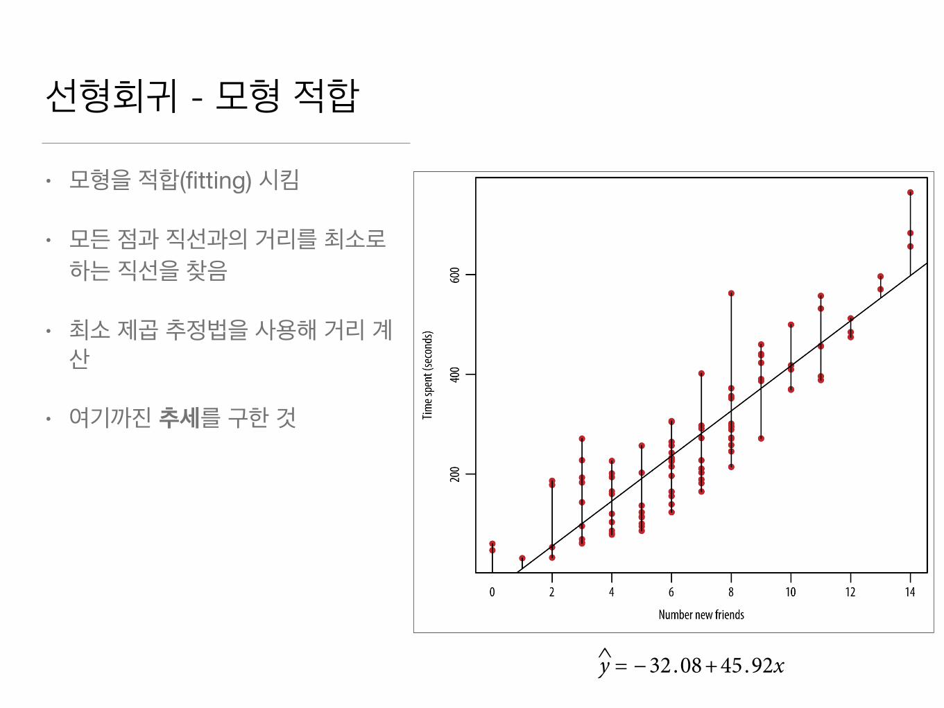
선형회귀 - 모형 적합
• 모형을 적합(fitting) 시킴
• 모든 점과 직선과의 거리를 최소로 하는 직선을 찾음
• 최소 제곱 추정법을 사용해 거리 계산
• 여기까진 추세를 구한 것
Figure 3-4. The line closest to all the points
To find this line, you’ll define the “residual sum of squares” (RSS),denoted RSS β , to be:
RSS β = ∑i yi − βxi2
where i ranges over the various data points. It is the sum of all thesquared vertical distances between the observed points and any givenline. Note this is a function of β and you want to optimize with respectto β to find the optimal line.
To minimize RSS β = y − βx t y − βx , differentiate it with respect toβ and set it equal to zero, then solve for β . This results in:
β = xt x −1xt y
62 | Chapter 3: Algorithms
www.it-ebooks.info
Here the little “hat” symbol on top of the β is there to indicate that it’sthe estimator for β. You don’t know the true value of β; all you have isthe observed data, which you plug into the estimator to get an estimate.
To actually fit this, to get the βs, all you need is one line of R code whereyou’ve got a column of y’s and a (single) column of x’s:
model <- lm(y ~ x)
So for the example where the first few rows of the data were:
x y
7 276
3 43
4 82
6 136
10 417
9 269
The R code for this would be:> model <- lm (y~x)> model
Call:lm(formula = y ~ x)
Coefficients:(Intercept) x -32.08 45.92
> coefs <- coef(model)> plot(x, y, pch=20,col="red", xlab="Number new friends", ylab="Time spent (seconds)")> abline(coefs[1],coefs[2])
And the estimated line is y = −32.08+45.92x, which you’re welcometo round to y = −32+46x, and the corresponding plot looks like thelefthand side of Figure 3-5.
Three Basic Algorithms | 63
www.it-ebooks.info
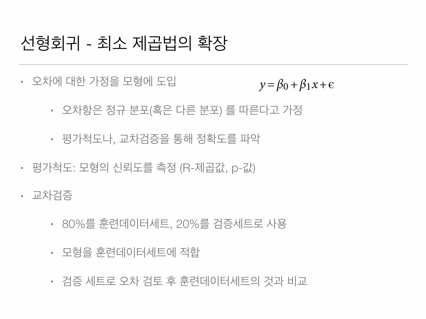
선형회귀 - 최소 제곱법의 확장
• 오차에 대한 가정을 모형에 도입
• 오차항은 정규 분포(혹은 다른 분포) 를 따른다고 가정
• 평가척도나, 교차검증을 통해 정확도를 파악
• 평가척도: 모형의 신뢰도를 측정 (R-제곱값, p-값)
• 교차검증
• 80%를 훈련데이터세트, 20%를 검증세트로 사용
• 모형을 훈련데이터세트에 적합
• 검증 세트로 오차 검토 후 훈련데이터세트의 것과 비교
righthand side of Figure 3-5 that for a fixed value of x = 5, there isvariability among the time spent on the site. You want to capture thisvariability in your model, so you extend your model to:
y = β0 + β1x +ϵ
where the new term ϵ is referred to as noise, which is the stuff that youhaven’t accounted for by the relationships you’ve figured out so far. It’salso called the error term—ϵ represents the actual error, the differencebetween the observations and the true regression line, which you’llnever know and can only estimate with your βs.
One often makes the modeling assumption that the noise is normallydistributed, which is denoted:
ϵ∼N 0,σ2
Note this is sometimes not a reasonable assumption. If youare dealing with a known fat-tailed distribution, and if yourlinear model is picking up only a small part of the value ofthe variable y, then the error terms are likely also fat-tailed.This is the most common situation in financial modeling.That’s not to say we don’t use linear regression in finance,though. We just don’t attach the “noise is normal” assumptionto it.
With the preceding assumption on the distribution of noise, this mod‐el is saying that, for any given value of x, the conditional distributionof y given x is p y x ∼N β0 + β1x,σ2 .
So, for example, among the set of people who had five new friends thisweek, the amount of the time they spent on the website had a normaldistribution with a mean of β0 + β1 *5 and a variance of σ2, and you’regoing to estimate your parameters β0,β1,σ from the data.
How do you fit this model? How do you get the parameters β0,β1,σfrom the data?
Three Basic Algorithms | 65
www.it-ebooks.info

If the mean squared errors are approximately the same, then ourmodel generalizes well and we’re not in danger of overfitting. SeeFigure 3-6 to see what this might look like. This approach is highlyrecommended.
Figure 3-6. Comparing mean squared error in training and test set,taken from a slide of Professor Nando de Freitas; here, the groundtruth is known because it came from a dataset with data simulatedfrom a known distribution
Other models for error termsThe mean squared error is an example of what is called a loss func‐tion. This is the standard one to use in linear regression because it givesus a pretty nice measure of closeness of fit. It has the additional de‐sirable property that by assuming that εs are normally distributed, wecan rely on the maximum likelihood principle. There are other lossfunctions such as one that relies on absolute value rather than squar‐ing. It’s also possible to build custom loss functions specific to yourparticular problem or context, but for now, you’re safe with using meansquare error.
68 | Chapter 3: Algorithms
www.it-ebooks.info

선형회귀 - 최소 제곱법의 확장
• 더 많은 예측 변수 추가(다중 선형회귀)
• 예측변수를 변환
Adding other predictors. What we just looked at was simple linear re‐gression—one outcome or dependent variable and one predictor. Butwe can extend this model by building in other predictors, which iscalled multiple linear regression:
y = β0 + β1x1 + β2x2 + β3x3 +ϵ .
All the math that we did before holds because we had expressed it inmatrix notation, so it was already generalized to give the appropriateestimators for the β. In the example we gave of predicting time spenton the website, the other predictors could be the user’s age and gender,for example. We’ll explore feature selection more in Chapter 7, whichmeans figuring out which additional predictors you’d want to put inyour model. The R code will just be:
model <- lm(y ~ x_1 + x_2 + x_3)
Or to add in interactions between variables:model <- lm(y ~ x_1 + x_2 + x_3 + x2_*x_3)
One key here is to make scatterplots of y against each of the predictorsas well as between the predictors, and histograms of y x for variousvalues of each of the predictors to help build intuition. As with simplelinear regression, you can use the same methods to evaluate yourmodel as described earlier: looking at R2, p-values, and using trainingand testing sets.
Transformations. Going back to one x predicting one y, why did weassume a linear relationship? Instead, maybe, a better model would bea polynomial relationship like this:
y = β0 + β1x + β2x2 + β3x3
Wait, but isn’t this linear regression? Last time we checked, polyno‐mials weren’t linear. To think of it as linear, you transform or createnew variables—for example, z = x2—and build a regression modelbased on z. Other common transformations are to take the log or topick a threshold and turn it into a binary predictor instead.
If you look at the plot of time spent versus number friends, the shapelooks a little bit curvy. You could potentially explore this furtherby building up a model and checking to see whether this yields animprovement.
Three Basic Algorithms | 69
www.it-ebooks.info

선형회귀 - 검토
• 가정 • 선형성
• 오차항은 평균이 0인 정규분포
• 오차항은 서로 독립
• 오차항은 모든 x에 대해 동일한 분산을 가짐
• 모형에 포함된 예측변수는 올바른 예측변수
• 선형회귀를 사용하는 이유 • 다른 변수들은 다 알고 하나의 변수에 대해 예측하려 할 때
• 둘 혹은 여럿 간의 관계를 설명하거나 이해하려 할 때

k-근접이웃(k-NN)
• 이미 분류한 많은 객체가 있을 때 아직 분류되지 않은 객체에 자동으로 분류명을 붙이고자 할 때 사용
• 아직 분류되지 않을 것과 가장 유사한 것들을 찾아내어 그것들의 분류명을 보고 다수결에 의해 분류명을 부여
• 지도 학습의 일종
• 결정해야 할 것
• 유사도/근접성을 어떻게 정의 할 것인가?
• 몇 명의 이웃을 선택해서 투표하게 할 것인가? (k값)

Make sense? Let’s try it out with a more realistic example.Example with credit scoresSay you have the age, income, and a credit category of high or low fora bunch of people and you want to use the age and income to predictthe credit label of “high” or “low” for a new person.
For example, here are the first few rows of a dataset, with income rep‐resented in thousands:
age income credit69 3 low66 57 low49 79 low49 17 low58 26 high44 71 high
You can plot people as points on the plane and label people with anempty circle if they have low credit ratings, as shown in Figure 3-7.
Figure 3-7. Credit rating as a function of age and income
Three Basic Algorithms | 73
www.it-ebooks.info
What if a new guy comes in who is 57 years old and who makes$37,000? What’s his likely credit rating label? Look at Figure 3-8. Basedon the other people near him, what credit score label do you think heshould be given? Let’s use k-NN to do it automatically.
Figure 3-8. What about that guy?
Here’s an overview of the process:
1. Decide on your similarity or distance metric.2. Split the original labeled dataset into training and test data.3. Pick an evaluation metric. (Misclassification rate is a good one.
We’ll explain this more in a bit.)4. Run k-NN a few times, changing k and checking the evaluation
measure.5. Optimize k by picking the one with the best evaluation measure.6. Once you’ve chosen k, use the same training set and now create a
new test set with the people’s ages and incomes that you have no
74 | Chapter 3: Algorithms
www.it-ebooks.info

k-근접이웃 - 절차
1. 유사도 또는 거리척도를 결정한다
• 단위 문제는 아주 중요함 (한 변수가 지배하지 않게 단위를 적절히 설정)
• 데이터 형태에 따라 여러 유사도 중 적합한 것을 선택 (모르면 구글링으로...)
2. 분류명이 있는 원래의 데이터들을 훈련데이터세트와 검증세트로 나눈다
• 검증 세트의 실제 분류명을 모르는 것 처럼 가정해서 검증 진행
3. 평가척도의 선택
• 보편적인 방법이 없음 => 해당 분야의 전문지식 사용
• 민감도와 특이도 간 적절한 균형이 필요
• 정밀도와 정확도 역시 사용 가능

ConditionPositive
ConditionNegative
Test outcomePositive True-Positive False-Positive
Test OutcomeNegative False-Negative True-Negative
예측값
실제값
참고링크: Sensitivity and specificity

k-근접이웃 - 절차
4. k 값을 변화시키면서 k-NN을 여러번 수행한 후 각 평가척도 값 계산
5. 평가척도가 가장 좋을 때의 k값을 최적값으로 한다.
6. k값이 정해졌으면 이 훈련데이터세트를 사용해서 분류명을 예측하고자 하는 검증 세트를 만든다.

k-근접이웃 - 모형화 과정에서의 가정
• 비모수적 접근방법: 모형화 가정 없음, 모수추정 하지 않음
• 데이터 간의 ‘거리’ 개념을 사용할 수 있는 특정 공간을 정의
• 훈련데이터세트는 두 개 이상의 분류를 가짐
• 이웃의 수 k를 선택
• 관측된 특징과 분류명은 연관성이 있다고 가정

k-평균법(k-means)
• 데이터를 k개로 군집화 하면서 정답을 만들어가는 알고리즘
• 목표는 사용자의 유사점을 찾아서 그들을 세분하는 것
• 사용하는 이유
• 사용자에게 개인화된 경험 제공
• 서로 다른 집단 간 다른 모형 적용
• 계층적 모형화

have been shown to each user (the number of impressions) and howmany times each has clicked on an ad (number of clicks).
Figure 3-9 shows a simplistic picture that illustrates what this mightlook like.
Figure 3-9. Clustering in two dimensions; look at the panels in the leftcolumn from top to bottom, and then the right column from top tobottom
Visually you can see in the top-left that the data naturally falls intoclusters. This may be easy for you to do with your eyes when it’s onlyin two dimensions and there aren’t that many points, but when youget to higher dimensions and more data, you need an algorithm tohelp with this pattern-finding process. k-means algorithm looks forclusters in d dimensions, where d is the number of features for eachdata point.
Three Basic Algorithms | 83
www.it-ebooks.info

k-평균법 - 장단점
• 문제점
• k값의 선택은 과학적이 아닌 분석자의 감에 의지
• 수렴의 문제: 단일해가 존재하지 않을 수 있다
• 해석의 문제: 답이 전혀 도움이 되지 않을 수 있음(제일 큰 문제)
• 장점
• (다른 군집화 알고리즘에 비해) 빠르다
• 마케팅, 컴퓨터비전, 다른 모형의 출발점으로 널리 응용되고 있다

대규모 데이터의 모형화와 알고리즘
• 모형을 규모에 맞게 확장해야 함
• 여러 차례 반복 수행에 기반을 둔 전통적인 접근방식은 적절하지 않음 => 비용이 높기 때문
• 현대적인 병렬 컴퓨팅 능력 활용: 멀티코어 프로세서, GPU, 컴퓨터 클러스터 등


![[동그라미재단] 2014ㄱ찾기_에어_CSS 입문](https://img.pdfslide.tips/doc/110x75/55d59e97bb61eb7b778b463b/-2014css-.jpg)