CUSUM ANOMALY DETECTION

1

THE CUSUM ANOMALY DETECTION ALGORITHM WAS CREATED IN RESPONSE TO THE NEED FOR AN AUTOMATIZED METHOD OF SEARCHING M-LAB’S VAST DATABASE OF NETWORK DIAGNOSTIC TEST RESULTS NOT FOR SINGLE OUTLIER POINTS, BUT FOR A SERIES OF UNUSUALLY HIGH OR LOW MEASUREMENTS. IT WAS DEVELOPED DURING THE COURSE OF A THREE MONTH LONG “OUTREACHY” INTERNSHIP AT MEASUREMENT LAB IN THE SUMMER OF 2015.

WHY WAS CAD CREATED?

2

3

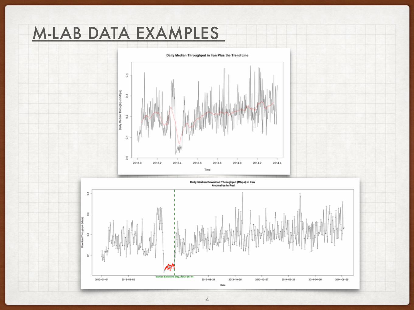
M-LAB DATA EXAMPLES

4

260

280

300

320

340

360

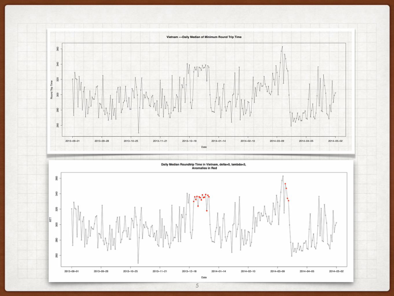
Vietnam −−Daily Median of Minimum Round Trip Time

Date

Rou

nd T

rip T

ime

2013−09−01 2013−09−28 2013−10−25 2013−11−21 2013−12−18 2014−01−14 2014−02−10 2014−03−09 2014−04−05 2014−05−02

5

6

CUSUM CHARTS

• It is a statistical control chart • It is a graph that is used to show how a process changes over

time. • It has a center line for the average • It has an upper control and a lower control line • The CUSUM chart uses four parameters:

1. the expected mean of the process 2. the expected standard deviation of the process 3. the size of the shift that is to be detected — k 4. the control limit — H

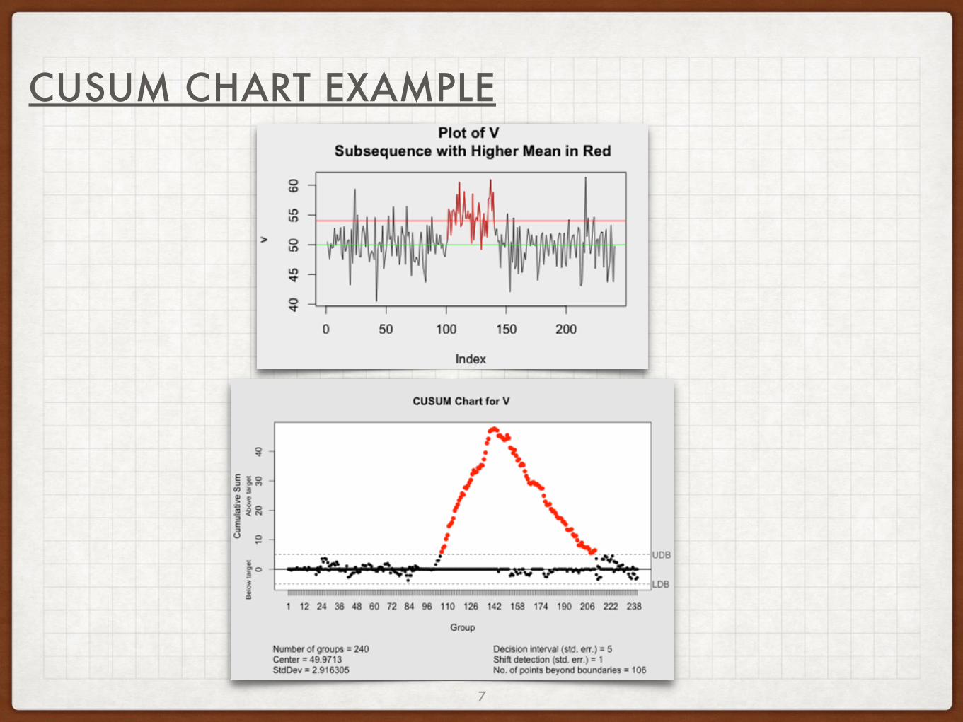
CUSUM CHART EXAMPLE

7

8

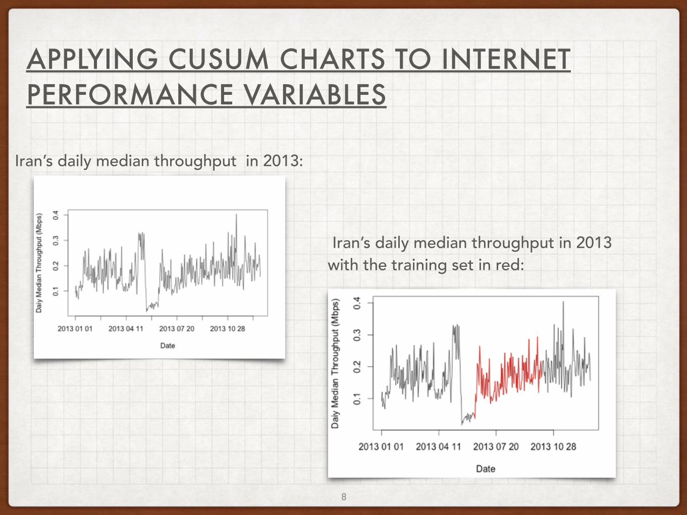
APPLYING CUSUM CHARTS TO INTERNET PERFORMANCE VARIABLES

Iran’s daily median throughput in 2013:

Iran’s daily median throughput in 2013 with the training set in red:

9

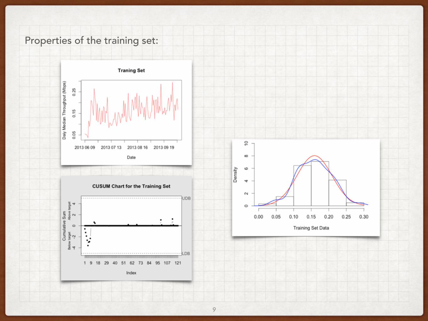
Properties of the training set:

10

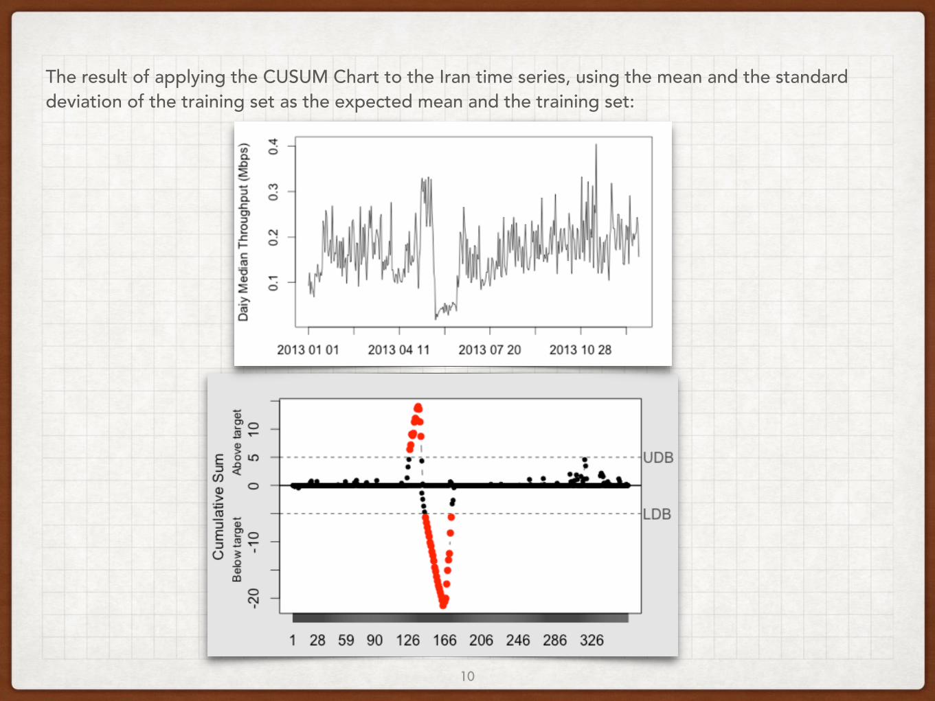
The result of applying the CUSUM Chart to the Iran time series, using the mean and the standard deviation of the training set as the expected mean and the training set:

11

CAD AND ITS DESIGN

OVERVIEW

The implementation of CAD was written in R and it uses the qcc* package to find the CUSUM chart of a time series. CAD uses the sliding window technique. For each window, CAD searches the time series along the window for a training set. If one is found, CAD applies the CUSUM chart to the entire time series along the window. After interpreting the results of the CUSUM chart, some of the points are designated as possible anomalies. This procedure is repeated for every window down the length of the time series. The output of the process is the indices of the anomalies within the time series and a graph of the time series with anomalies in red.

*Scrucca, L. (2004). qcc: an R package for quality control charting and statistical process control. R News 4/1, 11-17.

12

TUNING PARAMETERS

CAD is mostly automated, however, there are still a few parameters that, although they have default values, can nonetheless be adjusted by the user. These are:

• lambda: the minimum length of the anomalous subsequences that CAD should detect; its default value is 5. • delta: an offset added to the CUSUM parameter K; its default value is 3. • type: the choices for this parameter are upper or lower. It determines the type of anomaly CAD should search for.

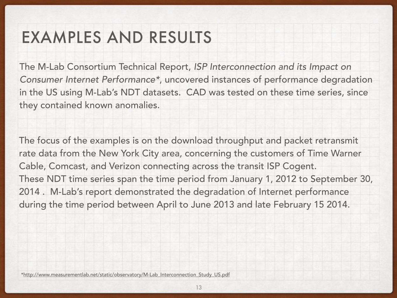
EXAMPLES AND RESULTS

13

The M-Lab Consortium Technical Report, ISP Interconnection and its Impact on Consumer Internet Performance*, uncovered instances of performance degradation in the US using M-Lab’s NDT datasets. CAD was tested on these time series, since they contained known anomalies.

*http://www.measurementlab.net/static/observatory/M-Lab_Interconnection_Study_US.pdf

The focus of the examples is on the download throughput and packet retransmit rate data from the New York City area, concerning the customers of Time Warner Cable, Comcast, and Verizon connecting across the transit ISP Cogent. These NDT time series span the time period from January 1, 2012 to September 30, 2014 . M-Lab’s report demonstrated the degradation of Internet performance during the time period between April to June 2013 and late February 15 2014.

14

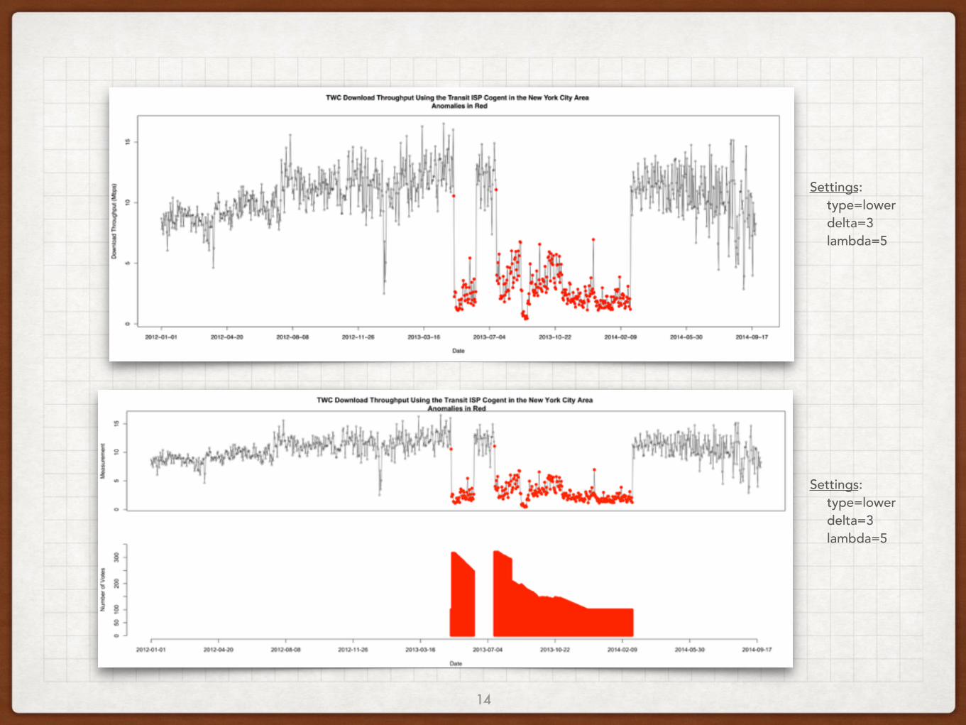
Settings: type=lower delta=3 lambda=5

Settings: type=lower delta=3 lambda=5

15

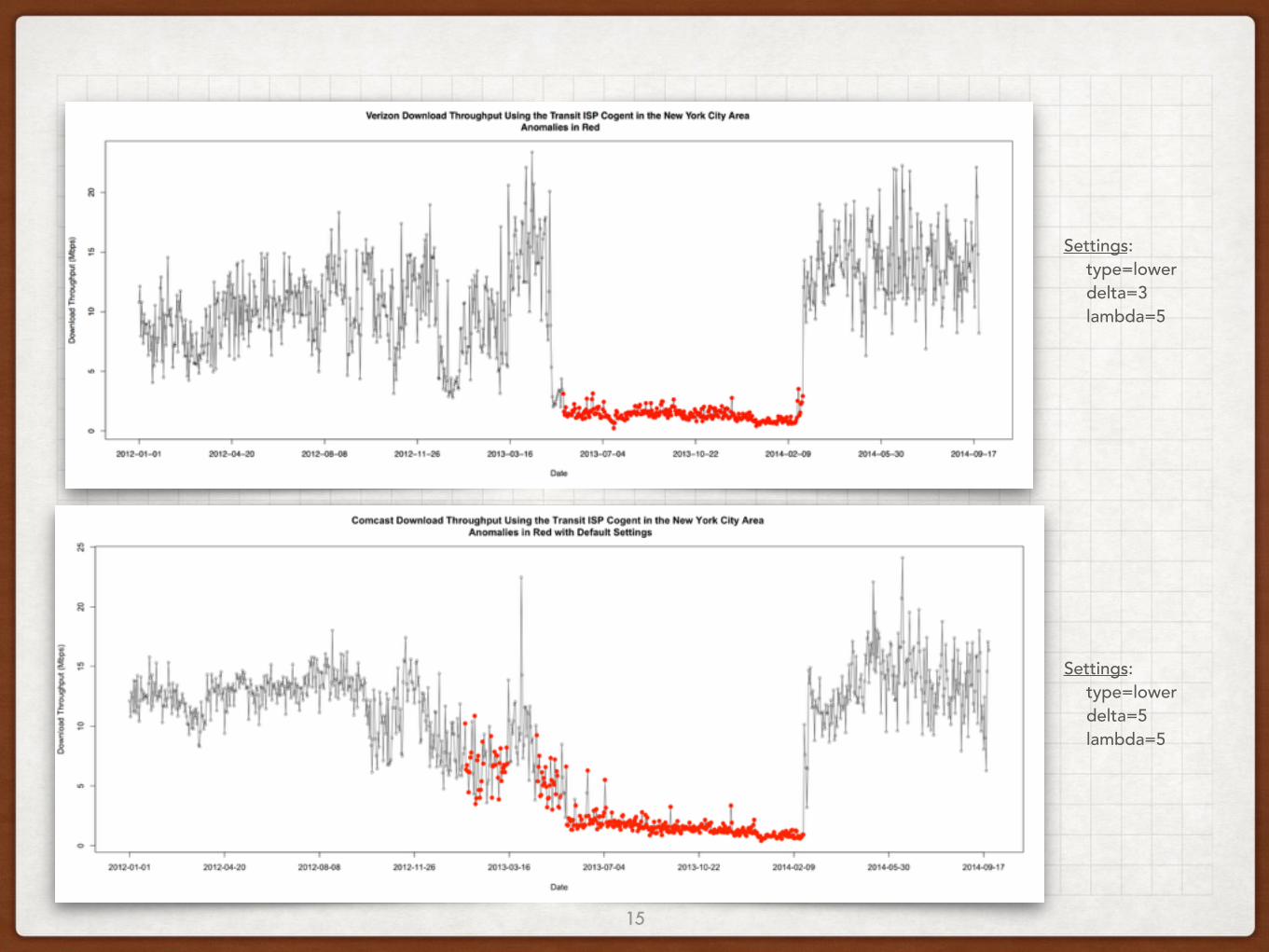
Settings: type=lower delta=3 lambda=5

Settings: type=lower delta=5 lambda=5

16

Settings: type=upper delta=3 lambda=1

Settings: type=upper delta=3 lambda=3

17

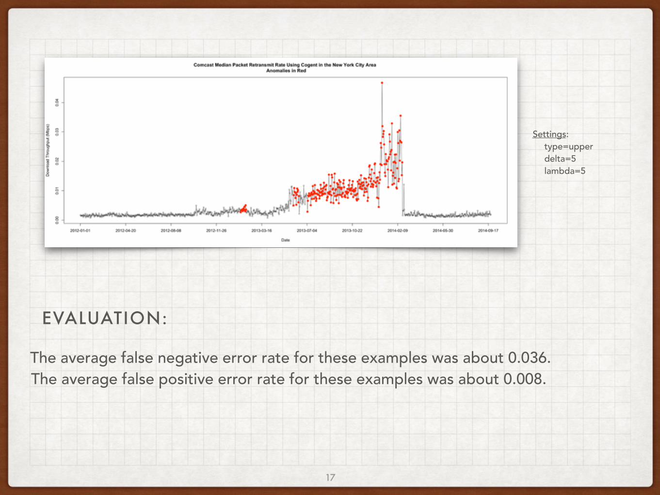
Settings: type=upper delta=5 lambda=5

The average false negative error rate for these examples was about 0.036. The average false positive error rate for these examples was about 0.008.

EVALUATION:

CONCLUSION & FUTURE WORK

• The CAD method works well for discovering anomalies in network performance data, with a high rate of successful anomaly detection and a low rate of false positives

• CAD has not been tested outside a narrow scope

• CAD is an automatic process, but it does not provide a list of points that can be labeled anomalous with absolute certainty. It merely provides a potential list of anomalies that the user must assess and then adjust parameters as necessary.

• Future work will be focused on eliminating delta from the list of tunable parameters and finding a way to make this method into a map-reduce process

18