动态经济计量模型与时间序列模型

罗 凯2005.11.22

Notice

为防止丢失，上机作业统一交至助教 黄国华师兄 信箱

huangguohua@gsm.pku.edu.cn

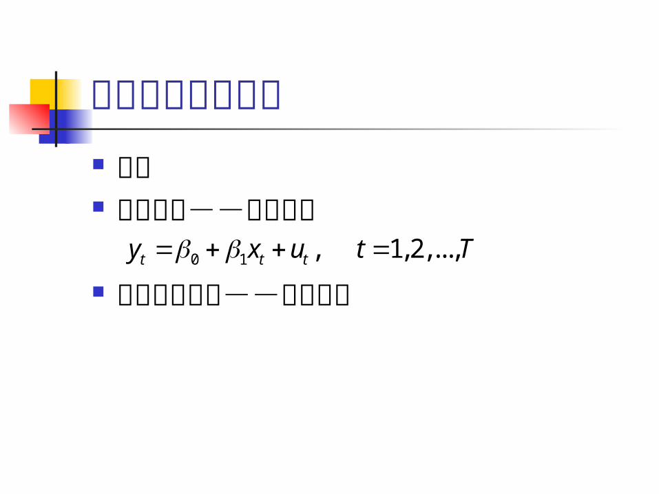
动态经济计量模型 时间 静态模型－－同期影响

分布滞后模型－－持续影响0 1 , 1, 2,...,t t ty x u t T

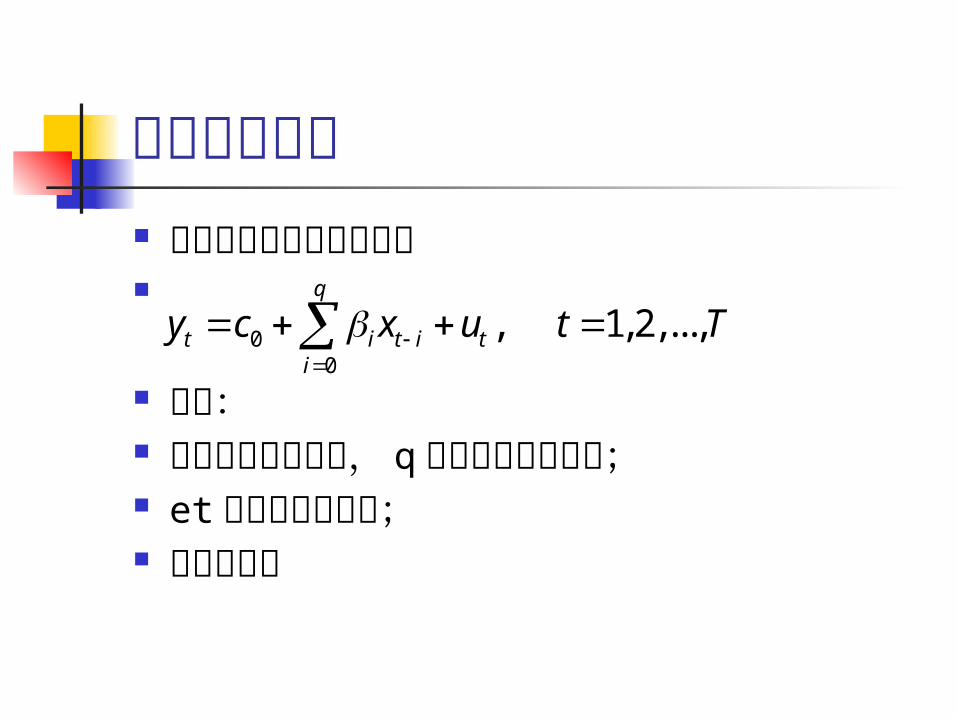
分布滞后模型 无约束有限分布滞后模型

困难： 时间序列期数有限， q 会过多占用自由度； et 自相关会很严重； 多重共线性

00

, 1, 2,...,q

t i t i ti

y c x u t T

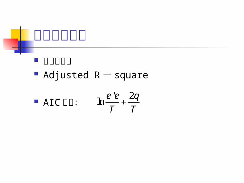
分布滞后模型 滞后期长度 Adjusted R － square

AIC 准则：' 2

lne e q

T T

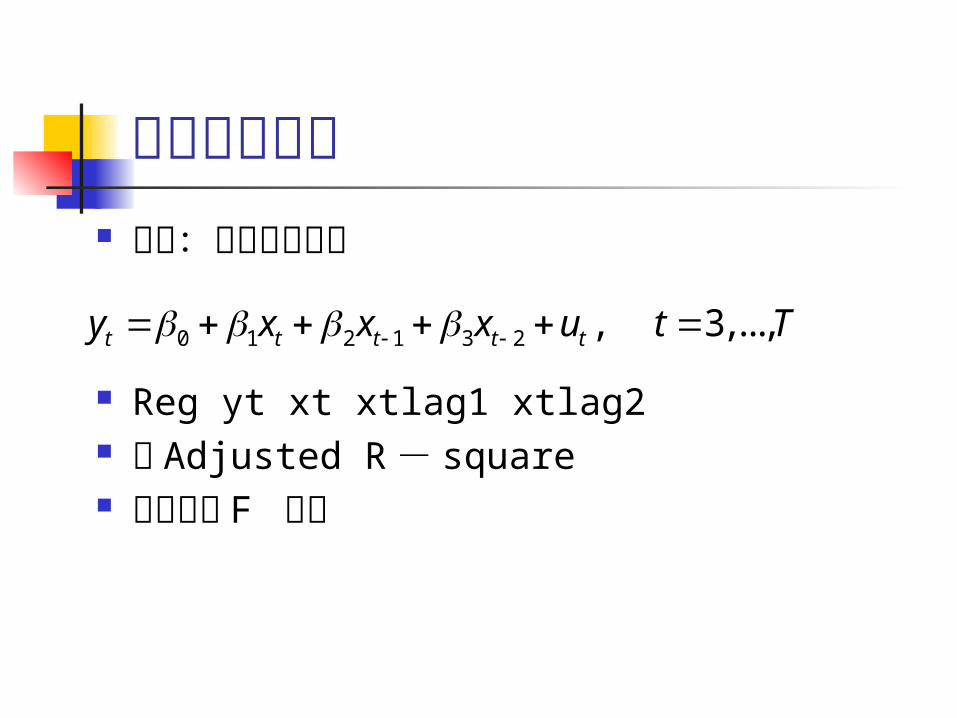
分布滞后模型 例如：两期滞后模型

Reg yt xt xtlag1 xtlag2 看 Adjusted R － square 进行序贯 F 检验

0 1 2 1 3 2 , 3,...,t t t t ty x x x u t T

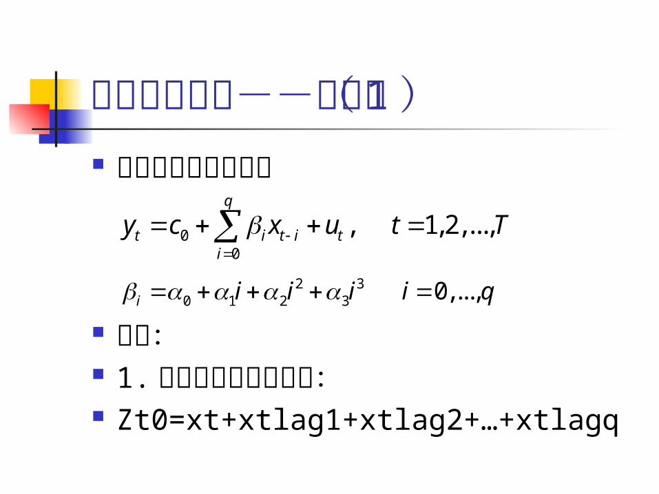
分布滞后模型－－方法（ 1 ） 多项式分布滞后模型

步骤： 1. 先定义新的解释变量： Zt0=xt+xtlag1+xtlag2+…+xtlagq

00

, 1, 2,...,q

t i t i ti

y c x u t T

2 3

0 1 2 3 0,...,i i i i i q

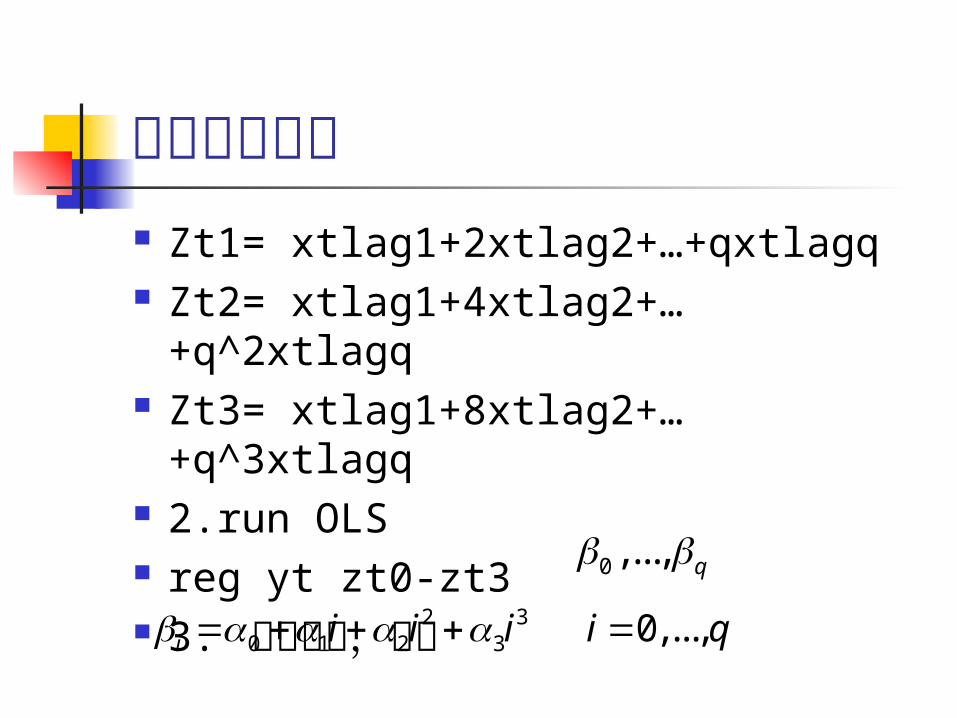
分布滞后模型 Zt1= xtlag1+2xtlag2+…+qxtlagq Zt2= xtlag1+4xtlag2+…

+q^2xtlagq Zt3= xtlag1+8xtlag2+…

+q^3xtlagq 2.run OLS reg yt zt0-zt3 3. 根据下式，回求

0 ,..., q 2 3

0 1 2 3 0,...,i i i i i q

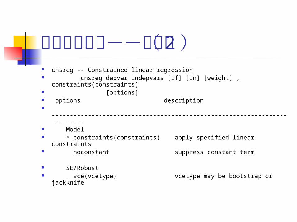
分布滞后模型－－方法（ 2 ） cnsreg -- Constrained linear regression cnsreg depvar indepvars [if] [in] [weight] ,

constraints(constraints) [options] options description -------------------------------------------------------------------------- Model * constraints(constraints) apply specified linear constraints noconstant suppress constant term

SE/Robust vce(vcetype) vcetype may be bootstrap or jackknife

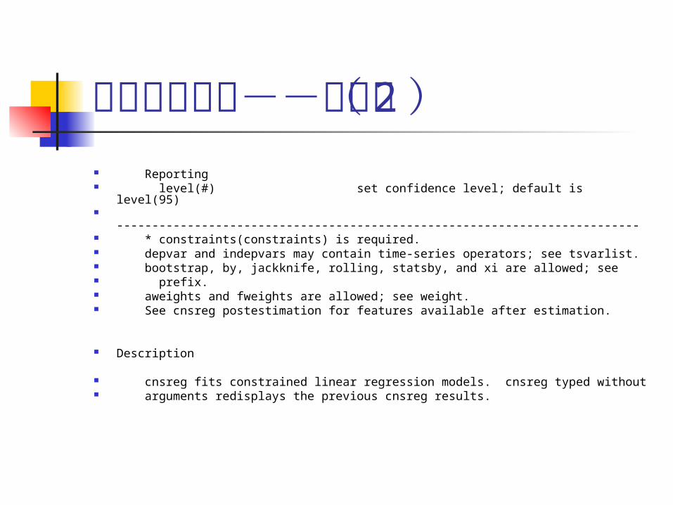
分布滞后模型－－方法（ 2 ） Reporting level(#) set confidence level; default is level(95) -------------------------------------------------------------------------- * constraints(constraints) is required. depvar and indepvars may contain time-series operators; see tsvarlist. bootstrap, by, jackknife, rolling, statsby, and xi are allowed; see prefix. aweights and fweights are allowed; see weight. See cnsreg postestimation for features available after estimation.

Description

cnsreg fits constrained linear regression models. cnsreg typed without arguments redisplays the previous cnsreg results.

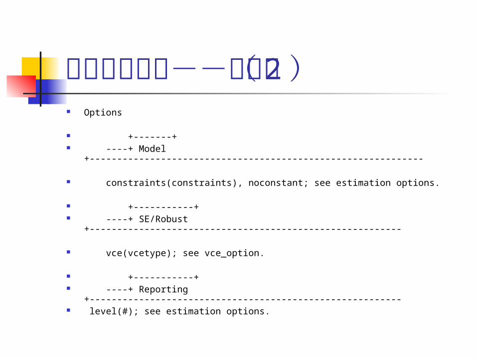
分布滞后模型－－方法（ 2 ） Options

+-------+ ----+ Model +-------------------------------------------------------------

constraints(constraints), noconstant; see estimation options.

+-----------+ ----+ SE/Robust +---------------------------------------------------------

vce(vcetype); see vce_option.

+-----------+ ----+ Reporting +--------------------------------------------------------- level(#); see estimation options.

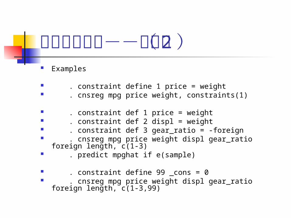
分布滞后模型－－方法（ 2 ） Examples

. constraint define 1 price = weight . cnsreg mpg price weight, constraints(1)

. constraint def 1 price = weight . constraint def 2 displ = weight . constraint def 3 gear_ratio = -foreign . cnsreg mpg price weight displ gear_ratio foreign length,

c(1-3) . predict mpghat if e(sample)

. constraint define 99 _cons = 0 . cnsreg mpg price weight displ gear_ratio foreign length,

c(1-3,99)

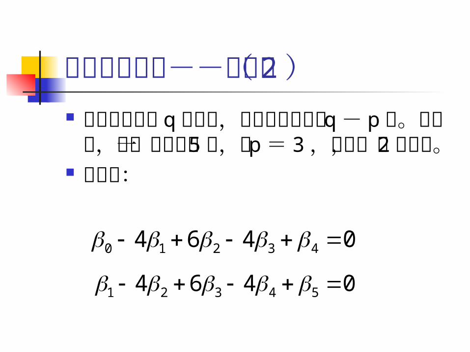
分布滞后模型－－方法（ 2 ） 如果原模型有 q 个滞后，则约束的个数

为 q － p 个。接上例，进一步设滞后 5期，因 p ＝ 3 ，因此，有 2 个约束。

依次为：

0 1 2 3 44 6 4 0

1 2 3 4 54 6 4 0

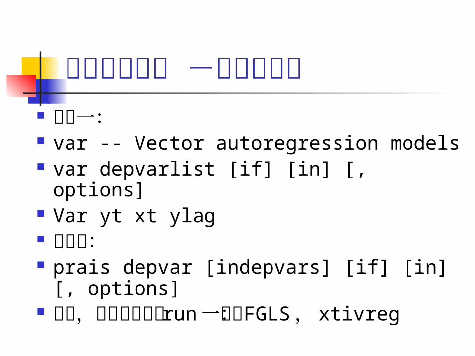
几何滞后模型 －自回归形式 方法一： var -- Vector autoregression models var depvarlist [if] [in] [, options] Var yt xt ylag 方法二： prais depvar [indepvars] [if] [in] [,

options] 此外，还是可以试着 run 一下：

FGLS ， xtivreg

几何滞后模型 －移动平均形式 主要方法：

非线性最小二乘法

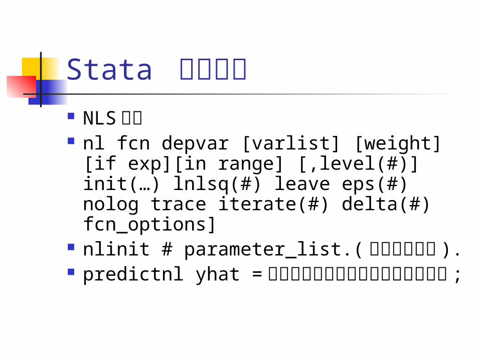
Stata 语句示例 NLS 语句 nl fcn depvar [varlist] [weight][if

exp][in range] [,level(#)] init(…) lnlsq(#) leave eps(#) nolog trace iterate(#) delta(#) fcn_options]

nlinit # parameter_list.( 给参数赋初值 ).

predictnl yhat = 将参数最终估计值带入的回归方程式 ;

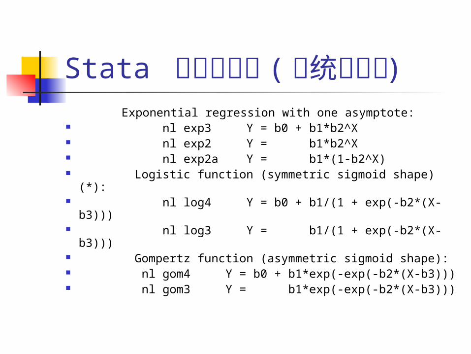
Stata 常用的函数 ( 系统已内设 ) Exponential regression with one asymptote: nl exp3 Y = b0 + b1*b2^X nl exp2 Y = b1*b2^X nl exp2a Y = b1*(1-b2^X) Logistic function (symmetric sigmoid shape)(*): nl log4 Y = b0 + b1/(1 + exp(-b2*(X-b3))) nl log3 Y = b1/(1 + exp(-b2*(X-b3))) Gompertz function (asymmetric sigmoid

shape): nl gom4 Y = b0 + b1*exp(-exp(-b2*(X-b3))) nl gom3 Y = b1*exp(-exp(-b2*(X-b3)))

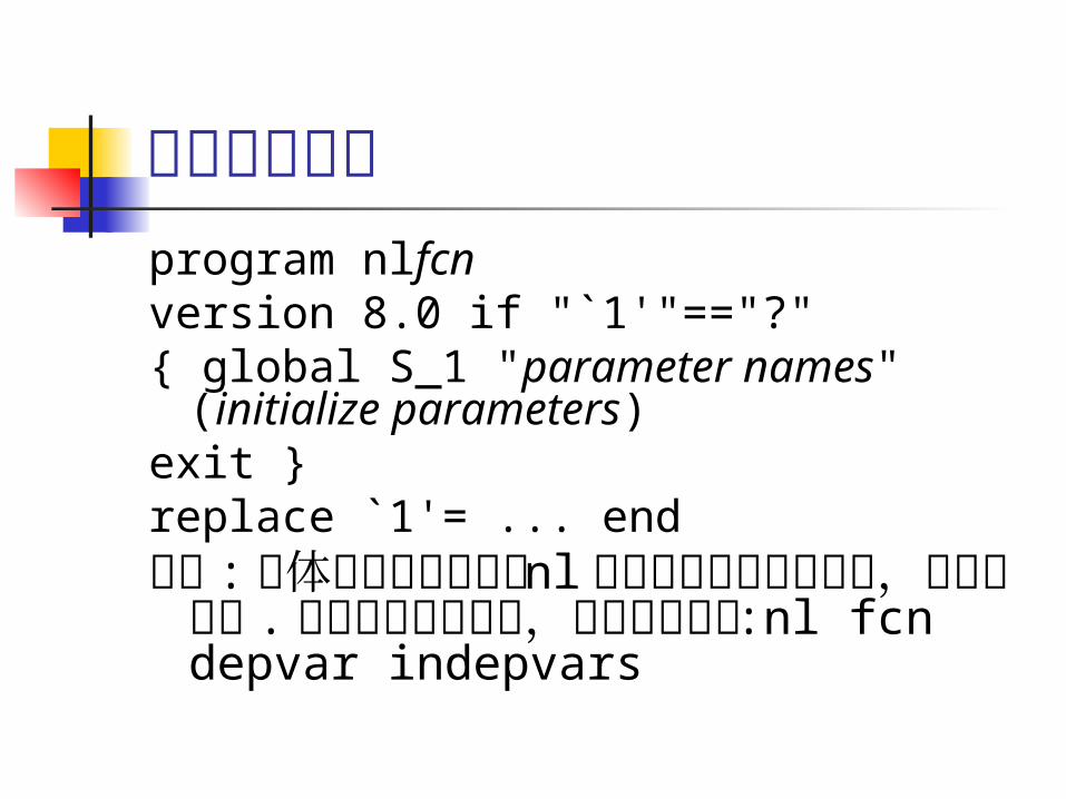
函数编程示例program nlfcn version 8.0 if "`1'"=="?" { global S_1 "parameter names"

(initialize parameters) exit } replace `1'= ... end 注意 : 具体函数名称前面的 nl 与函数名称

中间无空格，且不可去掉 . 以后可以直接调用，注意语句格式 :nl fcn depvar indepvars

动态回归模型 ARMAX 方法

或： ( 差分法 )

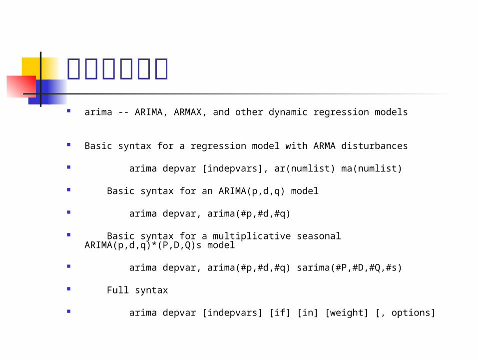
动态回归模型 arima -- ARIMA, ARMAX, and other dynamic regression models

Basic syntax for a regression model with ARMA disturbances

arima depvar [indepvars], ar(numlist) ma(numlist)

Basic syntax for an ARIMA(p,d,q) model

arima depvar, arima(#p,#d,#q)

Basic syntax for a multiplicative seasonal ARIMA(p,d,q)*(P,D,Q)s model

arima depvar, arima(#p,#d,#q) sarima(#P,#D,#Q,#s)

Full syntax

arima depvar [indepvars] [if] [in] [weight] [, options]

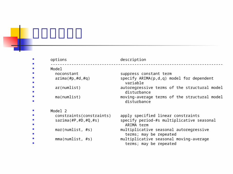
动态回归模型 options description -------------------------------------------------------------------------- Model noconstant suppress constant term arima(#p,#d,#q) specify ARIMA(p,d,q) model for dependent variable ar(numlist) autoregressive terms of the structural model disturbance ma(numlist) moving-average terms of the structural model disturbance

Model 2 constraints(constraints) apply specified linear constraints sarima(#P,#D,#Q,#s) specify period-#s multiplicative seasonal ARIMA term mar(numlist, #s) multiplicative seasonal autoregressive terms; may be repeated mma(numlist, #s) multiplicative seasonal moving-average terms; may be repeated

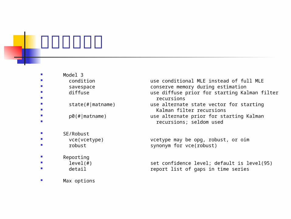
动态回归模型 Model 3 condition use conditional MLE instead of full MLE savespace conserve memory during estimation diffuse use diffuse prior for starting Kalman filter recursions state(#|matname) use alternate state vector for starting Kalman filter recursions p0(#|matname) use alternate prior for starting Kalman recursions; seldom used

SE/Robust vce(vcetype) vcetype may be opg, robust, or oim robust synonym for vce(robust)

Reporting level(#) set confidence level; default is level(95) detail report list of gaps in time series

Max options

动态回归模型 maximize_options control the maximization process; seldom used -------------------------------------------------------------------------- You must tsset your data before using arima; see tsset. depvar and indepvars may contain time-series operators; see tsvarlist. by, rolling, statsby, and xi may be used with arima; see prefix. iweights are allowed; see weights. See arima postestimation for features available after estimation.

Description

arima fits univariate models with time-dependent disturbances. arima fits a model of depvar on indepvars where the disturbances are allowed to follow a linear autoregressive moving-average (ARMA) specification. The dependent and independent variables may be differenced or seasonally differenced to any degree. When independent variables are included in the specification, such models are frequently called ARMAX models; and when independent variables are not specified, they reduce to Box-Jenkins autoregressive integrated moving-average (ARIMA) models in the dependent

动态回归模型 variable. Multiplicative seasonal ARIMA and ARMAX models can also be fitted. Missing data are allowed and are handled using the Kalman filter and methods outlined in [TS] arima.

In the full syntax, depvar is the variable being modeled, and the structural or regression part of the model is specified in indepvars. ar() and ma() specify the lags of autoregressive and moving-average terms, respectively; and mar() and mma() specify the multiplicative seasonal autoregressive and moving-average terms, respectively.

arima allows time-series operators in the dependent variable and independent variable lists, and it is often convenient to make extensive use of these operators; see dates for an extended discussion of time-series operators.

arima typed without arguments redisplays the previous estimates.

Options

动态回归模型 +-------+ ----+ Model +-------------------------------------------------------------

noconstant; see estimation options.

arima(#p,#d,#q) is an alternative, shorthand notation for specifying models with ARMA disturbances. The dependent variable and any independent variables are differenced #d times, 1 through #p lags of autocorrelations and 1 through #q lags of moving averages are included in the model. For example, the specification

. arima D.y, ar(1/2) ma(1/3)

is equivalent to

. arima y, arima(2,1,3)

The latter is easier to write for simple ARMAX and ARIMA models, but if gaps in the AR or MA lags are to be modeled, of if different operators are to be applied to independent variables, the first syntax

动态回归模型 is required.

ar(numlist) specifies the autoregressive terms of the structural model disturbance to be included in the model. For example, ar(1/3) specifies that lags of 1, 2, and 3 of the structural disturbance be included in the model; and ar(1 4) specifies that lags 1 and 4 be included, perhaps to account for additive quarterly effects.

If the model does not contain regressors, these terms can also be considered autoregressive terms for the dependent variable.

ma(numlist) specifies the moving-average terms to be included in the model. These are the terms for the lagged innovations (white-noise disturbances).

constraints(constraints); see estimation options for details.

If constraints are placed between structural model parameters and ARMA terms, the first few iterations may attempt steps into nonstationary areas. This can be ignored if the final solution is well within the

动态回归模型 bounds of stationary solutions.

+---------+ ----+ Model 2 +-----------------------------------------------------------

sarima(#P,#D,#Q,#s) is an alternative, shorthand notation for specifying the multiplicative seasonal components of models with ARMA disturbances. The dependent variable and any independent variables are lag-#s seasonally differenced #D times, and 1 through #P seasonal lags of autoregressive terms and 1 through #Q seasonal lags of moving-average terms are included in the model. For example, the specification

. arima DS12.y, ar(1/2) mar(1/2,12) mma(1/2,12)

is equivalent to

. arima y, arima(2,1,3) sarima(2,1,2,12)

mar(numlist,#s) specifies the lag-#s multiplicative seasonal autoregressive terms. For example, mar(1/2,12) requests that the

动态回归模型 first two lag-12 multiplicative seasonal autoregressive terms be included in the model.

mma(numlist,#s) specifies the lag-#s multiplicative seasonal moving-average terms. For example, mma(1 3,12) requests that the first and third (but not the second) lag-12 multiplicative seasonal moving-average terms be included in the model.

+---------+ ----+ Model 3 +-----------------------------------------------------------

condition specifies that conditional, rather than full, maximum likelihood estimates be produced. This estimation method is not appropriate for nonstationary series but may be preferable for long series or for models that have one or more long AR or MA lags. diffuse, p0(), and state0() may not be specified with condition. See [TS] arima for details.

savespace specifies that memory use be conserved by retaining only those variables required for estimation. The original dataset is restored

动态回归模型 after estimation. This option is rarely used and should be used only if there is insufficient space to fit a model without the option. Note, however, that arima requires considerably more temporary storage

diffuse specifies that a diffuse prior be used as a starting point for the during estimation than most estimation commands in Stata. Kalman filter recursions. Using diffuse, nonstationary models may be fitted with arima (see option p0() below; diffuse is equivalent to specifying p0(1e9)). See [TS] arima for details.

state0(#|matname) is a rarely used option that specifies an alternate initial state vector for starting the Kalman filter recursions. If # is specified, all elements of the vector are taken to be #. The default initial state vector is state0(0).

p0(#|matname) is a rarely specified option that can be used for nonstationary series or when an alternate prior for starting the Kalman recursions is desired; see [TS] arima for details.

+-----------+

动态回归模型 ----+ SE/Robust +---------------------------------------------------------

vce(vcetype); see vce_option.

robust; see estimation options.

For state-space models in general and ARMAX and ARIMA models in particular, the robust or quasi-maximum likelihood estimates (QMLE) of variance are robust to symmetric non-normality in the disturbances, including, as a special case, heteroskedasticity. The robust varianc estimates are not generally robust to functional misspecification of the structural or ARMA components of the model.

+-----------+ ----+ Reporting +---------------------------------------------------------

level(#); see estimation options.

detail specifies that a detailed list of any gaps in the series be reported, including gaps due to missing observations or missing data

动态回归模型 for the dependent variable or independent variables.

+-------------+ ----+ Max options +-------------------------------------------------------

maximize_options: difficult, technique(algorithm_spec), iterate(#), [no]log, trace, gradient, showstep, hessian, shownrtolerance, tolerance(#), ltolerance(#), gtolerance(#), nrtolerance(#), nonrtolerance(#), from(init_specs); see maximize.

These options are sometimes more important for ARIMA models than most maximum likelihood models because of potential convergence problems with ARIMA models, particularly if the specified model and the sample data imply a nonstationary model.

Several alternate optimization methods, such as Berndt-Hall-Hall-Hausman (BHHH) and Broyden-Fletcher-Goldfarb-Shanno (BFGS), are provided for arima models. Although arima models are not as difficult to optimize as ARCH models, their likelihoods are nevertheless generally not quadratic and often pose optimization

动态回归模型 difficulties; this is particularly true if a model is nonstationary or nearly nonstationary. Since each method approaches optimization differently, some problems can be successfully optimized by an alternate method when one method fails.

The following options are all related to maximization and are particularly important in fitting ARIMA models. technique(algorithm_spec) specifies the optimization technique to use to maximize the likelihood function.

technique(bhhh) specifies the Berndt-Hall-Hall-Hausman (BHHH) algorithm.

technique(dfp) specifies the Davidon-Fletcher-Powell (DFP) algorithm.

technique(bfgs) specifies the Broyden-Fletcher-Goldfarb-Shanno (BFGS) algorithm.

动态回归模型 technique(nr) specifies that Stata's modified Newton-Raphson (NR) algorithm.

You can specify multiple optimization methods. For example,

technique(bhhh 10 nr 20)

requests that the optimizer perform 10 BHHH iterations, switch to Newton-Raphson for 20 iterations, switch back to BHHH for 10 more iterations, and so on.

The default for arima is technique(bhhh 5 bfgs).

gtolerance(#) is a rarely used option that specifies a threshold for the relative size of the gradient; see maximize. The default gradient tolerance for arima is gtolerance(.05).

gtolerance(999) effectively disables the gradient criterion when convergence is difficult to achieve. If the optimizer becomes stuck with repeated "(backed up)" messages, the gradient probably

动态回归模型 still contains substantial values, but an uphill direction cannot be found for the likelihood. Using gtolerance(999) will often obtain results but it may be unclear whether the global maximum likelihood has been found. It is usually better to set the maximum number of iterations (see maximize) to the point where the optimizer appears to be stuck and then inspect the estimation results.

from(init_specs) specifies the starting values of the model coefficients; see maximize for a general discussion and syntax options.

The standard syntax for from() accepts a matrix, a list of values, or coefficient name value pairs; see maximize. In addition, arima accepts from(armab0), which sets the starting value for all ARMA paramters in the model to 0 prior to optimization.

ARIMA models may be sensitive to initial conditions and may have coefficent values that correspond to local maxima. The default starting values for arima are generally very good, particularly in

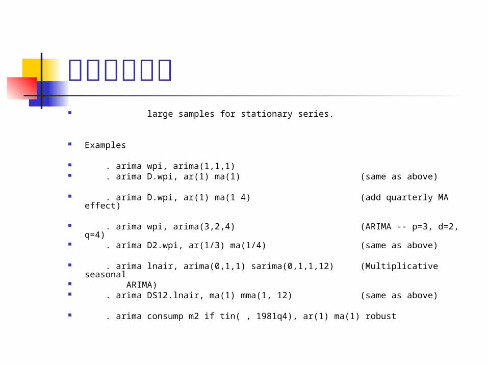
动态回归模型 large samples for stationary series.

Examples

. arima wpi, arima(1,1,1) . arima D.wpi, ar(1) ma(1) (same as above)

. arima D.wpi, ar(1) ma(1 4) (add quarterly MA effect)

. arima wpi, arima(3,2,4) (ARIMA -- p=3, d=2, q=4) . arima D2.wpi, ar(1/3) ma(1/4) (same as above)

. arima lnair, arima(0,1,1) sarima(0,1,1,12) (Multiplicative seasonal ARIMA) . arima DS12.lnair, ma(1) mma(1, 12) (same as above)

. arima consump m2 if tin( , 1981q4), ar(1) ma(1) robust

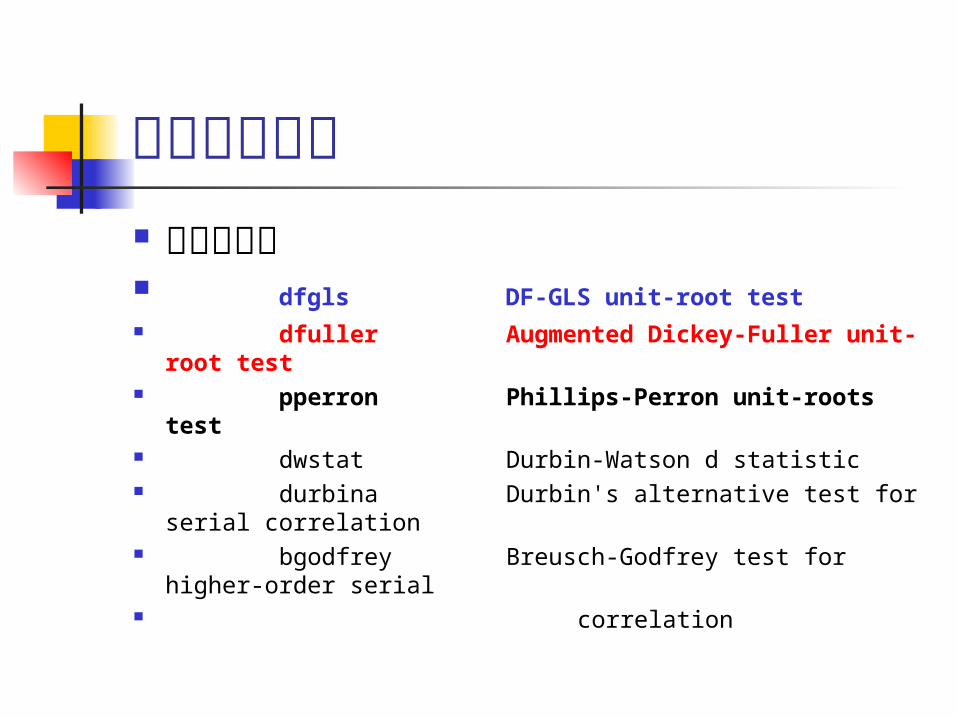
时间序列模型 单位根检验 dfgls DF-GLS unit-root test dfuller Augmented Dickey-Fuller unit-

root test pperron Phillips-Perron unit-roots test dwstat Durbin-Watson d statistic durbina Durbin's alternative test for serial

correlation bgodfrey Breusch-Godfrey test for higher-

order serial correlation

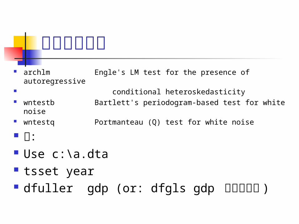
时间序列模型 archlm Engle's LM test for the presence of autoregressive conditional heteroskedasticity wntestb Bartlett's periodogram-based test for white noise wntestq Portmanteau (Q) test for white noise

例： Use c:\a.dta tsset year dfuller gdp (or: dfgls gdp 根据情况选 )

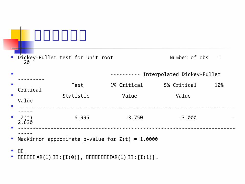
时间序列模型 Dickey-Fuller test for unit root Number of obs =

20

---------- Interpolated Dickey-Fuller --------- Test 1% Critical 5% Critical 10% Critical Statistic Value Value Value ------------------------------------------------------------------------------ Z(t) 6.995 -3.750 -3.000 -2.630 ------------------------------------------------------------------------------ MacKinnon approximate p-value for Z(t) = 1.0000

发散。 不遵循平稳的 AR(1) 过程 :[I(0)] ，其差分也不是平稳的 AR(1) 过程 :

[I(1)] 。

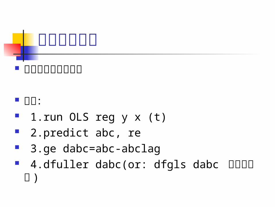
时间序列模型 协整和误差修正模型

步骤： 1.run OLS reg y x (t) 2.predict abc, re 3.ge dabc=abc-abclag 4.dfuller dabc(or: dfgls dabc 根据情况选 )

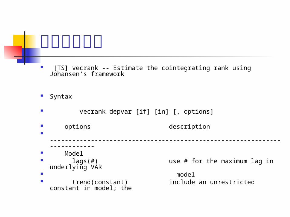
其他备用语句 [TS] vecrank -- Estimate the cointegrating rank using

Johansen's framework

Syntax

vecrank depvar [if] [in] [, options]

options description -------------------------------------------------------------------------- Model lags(#) use # for the maximum lag in underlying

VAR model trend(constant) include an unrestricted constant in

model; the

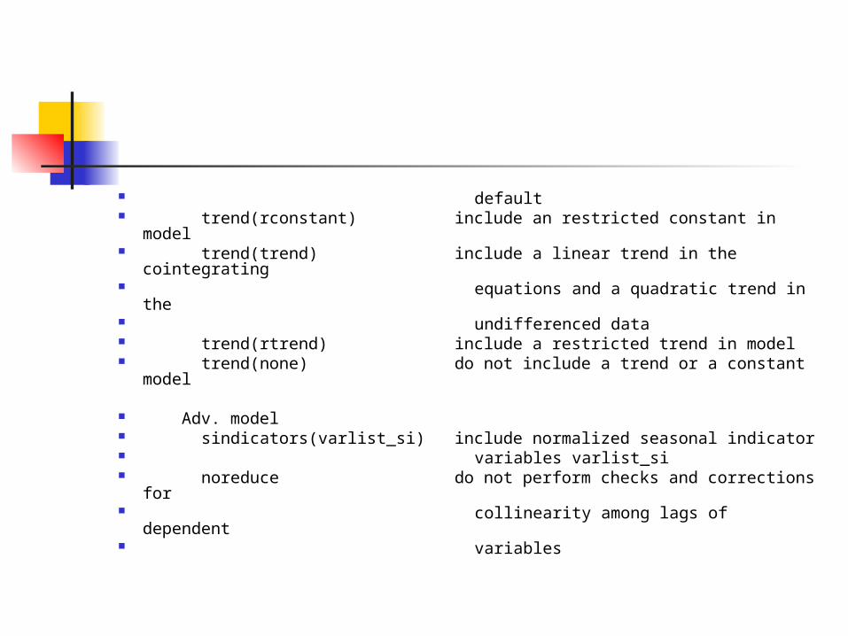
default trend(rconstant) include an restricted constant in model trend(trend) include a linear trend in the cointegrating equations and a quadratic trend in the undifferenced data trend(rtrend) include a restricted trend in model trend(none) do not include a trend or a constant model

Adv. model sindicators(varlist_si) include normalized seasonal indicator variables varlist_si noreduce do not perform checks and corrections for collinearity among lags of dependent variables

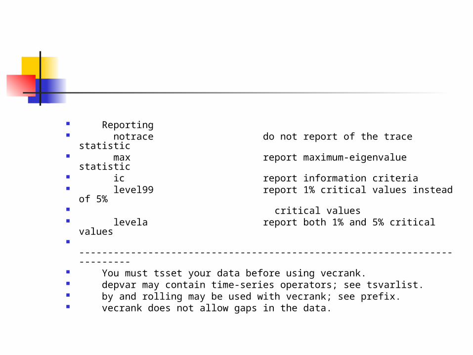
Reporting notrace do not report of the trace statistic max report maximum-eigenvalue statistic ic report information criteria level99 report 1% critical values instead of

5% critical values levela report both 1% and 5% critical values -------------------------------------------------------------------------- You must tsset your data before using vecrank. depvar may contain time-series operators; see tsvarlist. by and rolling may be used with vecrank; see prefix. vecrank does not allow gaps in the data.

Description

vecrank produces statistics used to determine the number of cointegrating

equations in a vector error-correction model (VECM).

Options

+-------+ ----+ Model +-------------------------------------------------------------

lags(#) specifies the number of lags in the VAR representation of the

model. The VECM will include one fewer lag of the first-differences.

The number of lags must be greater than zero but small enough so that

the degrees of freedom used up by the model are less than the number

of observations.

trend(trend_spec) specifies one of five trend specifications to include in

the model. See vec intro and vec for descriptions. The default is trend(constant).

+------------+ ----+ Adv. model +--------------------------------------------------------

sindicators(varlist_si) specifies normalized seasonal indicator variables

to be included in the model. The indicator variables specified in

this option must be normalized. If the indicators are not properly normalized, the likelihood-ratio-based tests for the number of cointegrating equations do not converge to the asymptotic distributions derived by Johansen. For details, see Methods and Formulas of [TS] vec. sindicators() cannot be specified with trend(none) or trend(rconstant).

noreduce causes vecrank to skip the checks and corrections for collinearity among the lags of the dependent variables. By default, vecrank checks if the current lag specification causes some of the regressions performed by vecrank to contain perfectly collinear variables and reduces the maximum lag until the perfect collinearity is removed. See Collinearity in [TS] vec for more information.

+-----------+ ----+ Reporting +---------------------------------------------------------

notrace requests that the output for the trace statistic not be displayed.

The default is to display the trace statistic.

max requests that the output for the maximum-eigenvalue statistic be

displayed. The default is to not display this output.

ic causes the output for the information criteria to be displayed. The

default is to not display this output.

level99 causes the 1% critical values to be displayed instead of the default 5% critical values.

levela causes both the 1% and the 5% critical values to be displayed.

Examples

. vecrank y i c, lags(5)

. vecrank y i c, lags(5) level99

. vecrank y i c, lags(5) max levela notrace

. vecrank y i c, lags(5) ic notrace