Embed Size (px)
Citation preview

© 2008 Pearson Addison Wesley. All rights reserved
Chapter Three
A Consumer’s Constrained Choice
家庭收支調查 _消費支出
© 2008 Pearson Addison Wesley. All rights reserved. 3-2
消費支出結構(%) 86年 96年 增減百分點
食品飲料費 25.7 24.2 -1.5
衣著鞋襪費 4.5 3.3 -1.2
房租、水電 25.1 23.5 -1.6
家具管理費 4.4 3.4 -1
醫療保健費 10 14.3 4.3
交通通訊費 10.4 12.5 2
娛樂教育費 13.1 12.5 -0.6
雜項支出 6.8 6.3 -0.5
資料來源:主計處 家庭收支調查 96 年新聞稿
家庭收支調查 _消費支出
© 2008 Pearson Addison Wesley. All rights reserved. 3-3
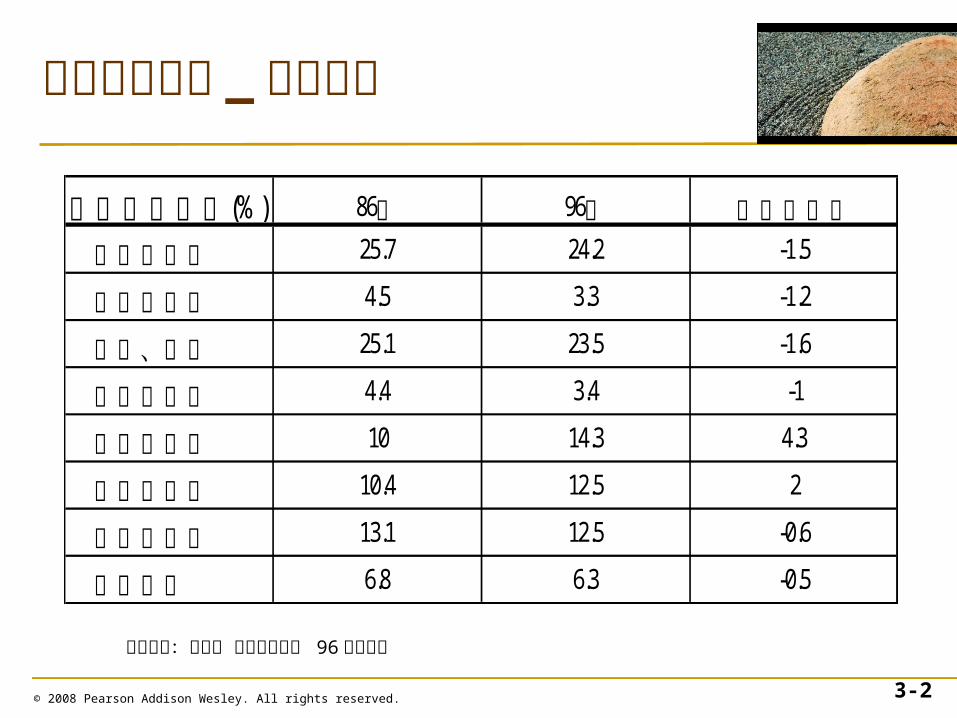
資料來源:主計處 家庭收支調查 96 年新聞稿
86 年消費支出結構 96 年消費支出結構
家庭收支調查 _消費性支出 _食品類項目表
© 2008 Pearson Addison Wesley. All rights reserved. 3-4
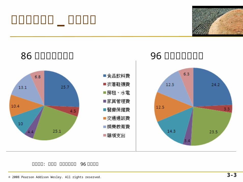
主食品 米、米製品,麥麵,雜糧,農牧戶自種自食設算。
副食品肉類,魚貝及水產品,蔬菜類,蛋類,油脂類,調味品類。農牧戶自種自食設算。
乳酪類奶粉,訂購鮮牛、羊奶,其他奶製品,如奶油、煉乳、養樂多.....等。
水果類 水果,自種自食設算,其他加工水果與乾果,檳榔。其他 茶,咖啡、可可,砂糖(方糖),糖果、冰淇淋等其他糖類。
婚生壽慶喪祭宴費凡上列各類食物因婚生壽慶喪祭及地區性拜拜而增加購買食品費金額,例如滿月油飯、蛋糕、喜餅、建醮宴客等 (初1、15拜拜之食品。
在外伙食費1.向現場有調理(煎煮炒炸、沖泡)之餐飲服務者,所購買可即時依消費者需求調整口味且供立即食用之餐飲費。2.平均每月搭伙:如學生餐費;就業;托兒所、幼稚園點心費。
Chapter Outline
• In this chapter, we examine four main topics.
– Preferences
– Utility
– Budget Constraint
– Constrained Consumer Choice
© 2008 Pearson Addison Wesley. All rights reserved. 3-5
© 2007 Pearson Addison-Wesley. All rights reserved. 3–6
Preferences
• To explain consumer behavior, economists assume that consumers have a set of tastes or preferences that they use to guide them in choosing between goods. These tastes differ substantially among individuals.
© 2007 Pearson Addison-Wesley. All rights reserved. 3–7
Properties of Consumer Preferences
• Economists make five critical assumptions about the properties of consumers’ preferences.
• For brevity, these properties are referred to as completeness, transitivity, more is better, continuity, and strict convexity.
© 2007 Pearson Addison-Wesley. All rights reserved. 3–8
Completeness
• The completeness property holds that, when facing a choice between any two bundles of goods, a consumer can rank them so that one and only one of the following relationships is true: The consumer prefers the first bundle to the second, prefers the second to the first, or is indifferent between them.
© 2007 Pearson Addison-Wesley. All rights reserved. 3–9
Transitivity
• The transitivity (or what some people refer to
as rationality) property is that a consumer’s
preferences over bundles is consistent in the
sense that, if the consumer weakly prefers Bundle z to Bundle y (like z at least as much as
y ) and weakly prefers Bundle y to Bundle x ,
the consumer also weakly prefers Bundle z to
Bundle x .
© 2007 Pearson Addison-Wesley. All rights reserved. 3–10
• good– a commodity for which more is preferred to
less, at least at some levels of consumption
• bad– something for which less is preferred to
more, such as pollution
• We now concentrate on goods.
More is Better
© 2007 Pearson Addison-Wesley. All rights reserved. 3–11
More is Better
• The more-is-better property holds that, all else the same, more of a commodity is better than less of it (always wanting more is known as nonsatiation).
Continuity
• The continuity property holds that if a consumer prefer Bundle a to Bundle b, then the consumer prefers Bundle c to b if c is very close to a.
• The purpose of this assumption is to rule out sudden preference reversals in response to small change in the characteristics of a bundle.
© 2007 Pearson Addison-Wesley. All rights reserved. 3–12
Strict Convexity
• Strict convexity of preferences means that consumers prefer averages to extremes.
• If Bundle a and Bundle b are distinct bundles and the consumer prefers both of these bundles to Bundle c, then the consumer prefers a weighted average of a and b, a + (1-)b (where 0 < < 1), to Bundle c.
© 2007 Pearson Addison-Wesley. All rights reserved. 3–13
© 2007 Pearson Addison-Wesley. All rights reserved. 3–14
Preference Maps
• One of the simplest ways to summarize information about a consumer’s preferences is to create a graphical interpretation—a map—of them.
© 2007 Pearson Addison-Wesley. All rights reserved. 3–15
• indifference curve– the set of all bundles of goods that a
consumer views as being equally desirable
• indifference map (or preference map)– a complete set of indifference curves that
summarize a consumer’s tastes or preferences
Preference Maps
© 2008 Pearson Addison Wesley. All rights reserved. 3-16
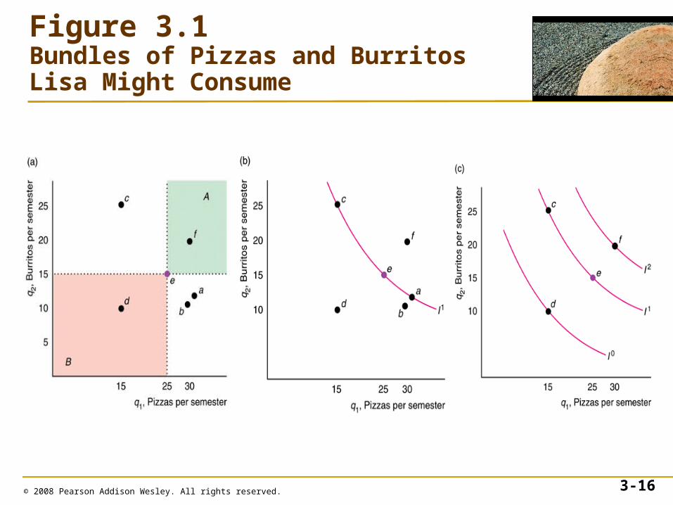
Figure 3.1Bundles of Pizzas and Burritos Lisa Might Consume
© 2007 Pearson Addison-Wesley. All rights reserved. 3–17
Indifference Curves
• All indifference curve maps must have five important properties:1. Bundles on indifference curves farther from
the origin are preferred to those on indifference curves closer to the origin.
2. There is an indifference curve through every possible bundle.
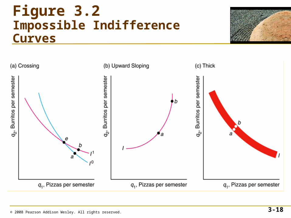
3. Indifference curves cannot cross.
4. Indifference curves slope downward.
5. Indifference curves cannot be thick
© 2008 Pearson Addison Wesley. All rights reserved. 3-18
Figure 3.2Impossible Indifference Curves
© 2007 Pearson Addison-Wesley. All rights reserved. 3–19
Utility
• Utility– a set of numerical values that reflect the
relative rankings of various bundles of goods
• Utility Function– the relationship between utility values and
every possible bundle of goods
© 2007 Pearson Addison-Wesley. All rights reserved. 3–20
Ordinal Preferences
• If we know only consumers’ relative rankings of bundles, our measure of pleasure is ordinal rather than cardinal. An ordinal measure is one that tells us the relative ranking of two things but not how much more one rank is than another.
• Because utility is an ordinal measure, we should not put any weight on the absolute differences between the utility associated with one bundle and another. We care only about the relative utility or ranking of the two bundles.
Utility and Indifference Curves
• In short, an indifference curve consists of all those bundles that correspond to a particular utility measure.
• A utility function is . This expression determines all those bundles of and that give her utility of pleasure.
© 2008 Pearson Addison Wesley. All rights reserved. 3-21
1q 2q U

© 2007 Pearson Addison-Wesley. All rights reserved. 3–22
Willingness to Substitute Between Goods
• Marginal Utility
– the slope of the utility function– the extra utility that a consumer gets from
consuming the last unit of a good–
11
1 Uq
Uq
ofutilitymarginal
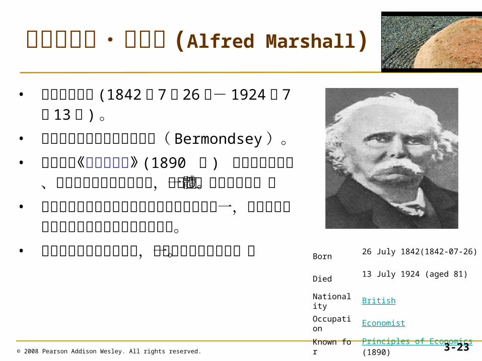
艾爾弗雷德 ·馬歇爾 (Alfred Marshall)
Born26 July 1842(1842-07-26)
Died13 July 1924 (aged 81)
Nationality British
Occupation Economist
Known for Principles of Economics (1890)
© 2008 Pearson Addison Wesley. All rights reserved. 3-23
• 英國經濟學家 (1842年 7月 26日-1924年 7月 13日 )。
• 出生在英國倫敦南岸的柏孟塞( Bermondsey)。
• 他的著作《經濟學原理》 (1890 的 ) 集中了供求理論、邊際效用理論和生產成本,形成了一個邏輯的整體。
• 這部著作使他成為當時的最顯赫的經濟學家之一,並在很長時間裡是英國大學科堂的經濟學課本。
• 馬歇爾曾任劍橋大學教授,凱恩斯是他的學生之一。
© 2007 Pearson Addison-Wesley. All rights reserved. 3–24
Willingness to Substitute Between Goods
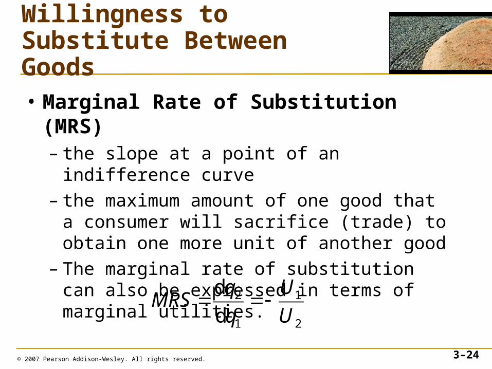
• Marginal Rate of Substitution (MRS)– the slope at a point of an indifference curve– the maximum amount of one good that a
consumer will sacrifice (trade) to obtain one more unit of another good
– The marginal rate of substitution can also be expressed in terms of marginal utilities.
2
1
1
2
d
d
U
U
q
qMRS
Willingness to Substitute Between Goods
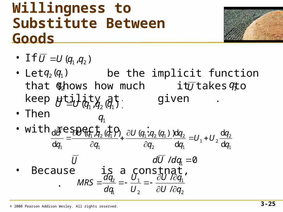
• If • Let be the implicit function that shows how
much it takes to keep utility at given .• Then • with respect to :
• Because is a constnat, .
© 2008 Pearson Addison Wesley. All rights reserved. 3-25
),( 21 qqUU )( 12 qq
2q U 1q
))(,( 121 qqqUU
1q
1
221
1
2
2
121
1
121
1 d
d
d
d))(,())(,(
d
d
q
qUU
q
q
q
qqqU
q
qqqU
q
U
U 0/ 1 dqUd
2
1
2
1
1
2
/
/
qU
qU
U
U
dq
dqMRS
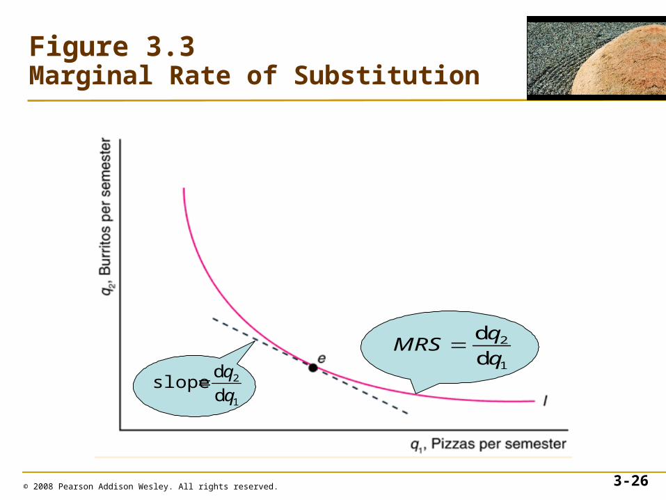
© 2008 Pearson Addison Wesley. All rights reserved. 3-26
Figure 3.3Marginal Rate of Substitution
1
2
d
d
q
qMRS
1
2
d
dslope
q
q

Solved Problem 3.2Cobb-Douglas Utility Function
• Suppose that Jackie has what is known as a Cobb-Douglas utility function:
Where is a positive constant, is the number of music CDs she buys a year, and is the number of movie DVDs she buys.
• What is her marginal rate of substitution?
© 2008 Pearson Addison Wesley. All rights reserved. 3-27
aaqqU 121
a 1q2q
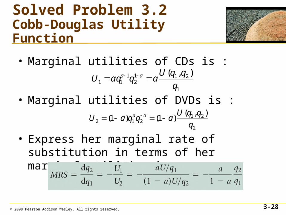
Solved Problem 3.2Cobb-Douglas Utility Function
• Marginal utilities of CDs is :
• Marginal utilities of DVDs is :
• Express her marginal rate of substitution in terms of her marginal utilities is :
© 2008 Pearson Addison Wesley. All rights reserved. 3-28
1
2112
111
),(
q
qqUaqaqU aa
2
21212
),()1()1(
q
qqUaqqaU aa
© 2007 Pearson Addison-Wesley. All rights reserved. 3–29
Curvature of Indifference Curves
• An indifference curve doesn’t have to be
convex, but casual observation suggests that
most people’s indifference curves are convex.
• When people have a lot of one good, they are
willing to give up a relatively large amount of it
to get a good of which they have relatively little.
However, after that first trade, they are willing to
give up less of the first good to get the same
amount more of the second good.
© 2007 Pearson Addison-Wesley. All rights reserved. 3–30
• This willingness to trade fewer burritos for one
more pizza as we move down and to the right
along the indifference curve reflects a
diminishing marginal rate of substitution:
The marginal rate of substitution (MRS)
approaches zero─becomes flatter or sloped─as
we move down and to the right along an
indifference curve.
Curvature of Indifference Curves
© 2007 Pearson Addison-Wesley. All rights reserved. 3–31
Curvature of Indifference Curves
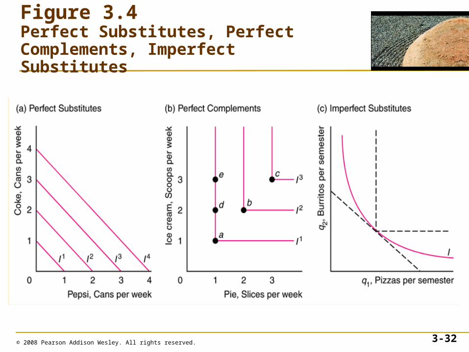
• Perfect Substitutes– goods that a consumer is completely
indifferent as to which to consume– U(C, G) = iC + jG
• Perfect Complements– goods that a consumer is interested in
consuming only in fixed proportions– U(A, V) = min(iA, jV)
© 2008 Pearson Addison Wesley. All rights reserved. 3-32
Figure 3.4Perfect Substitutes, Perfect Complements, Imperfect Substitutes
© 2007 Pearson Addison-Wesley. All rights reserved. 3–33
Budget Constraint
• Consumers maximize their well-being subject to constraints. The most important constraint most of us face in deciding what to consume is our personal budget constraint.
• For simplicity, we assume that each consumer has a fixed amount of money to spend now, so we can use the terms budget and income interchangeably.
Budget Constraint
• If Lisa spends all her budget, Y, on pizza and burritos, then
where p1q1 is the amount she spends on
pizzas and p2q2 is the amount she spends
on burritos.
© 2007 Pearson Addison-Wesley. All rights reserved. 3–34
© 2007 Pearson Addison-Wesley. All rights reserved. 3–35
Budget Constraint
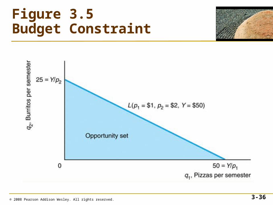
• Budget Line (or Budget Constraint )
– the bundles of goods that can be bought if
the entire budget is spent on those goods at
given prices
• Opportunity Set
– all the bundles a consumer can buy, including
all the bundles inside the budget constraint
and on the budget constraint
© 2008 Pearson Addison Wesley. All rights reserved. 3-36
Figure 3.5Budget Constraint
© 2007 Pearson Addison-Wesley. All rights reserved. 3–37
Slope of the Budget Constraint
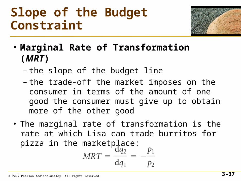
• Marginal Rate of Transformation (MRT)– the slope of the budget line– the trade-off the market imposes on the
consumer in terms of the amount of one good the consumer must give up to obtain more of the other good
• The marginal rate of transformation is the rate at which Lisa can trade burritos for pizza in the marketplace:
© 2007 Pearson Addison-Wesley. All rights reserved. 3–38
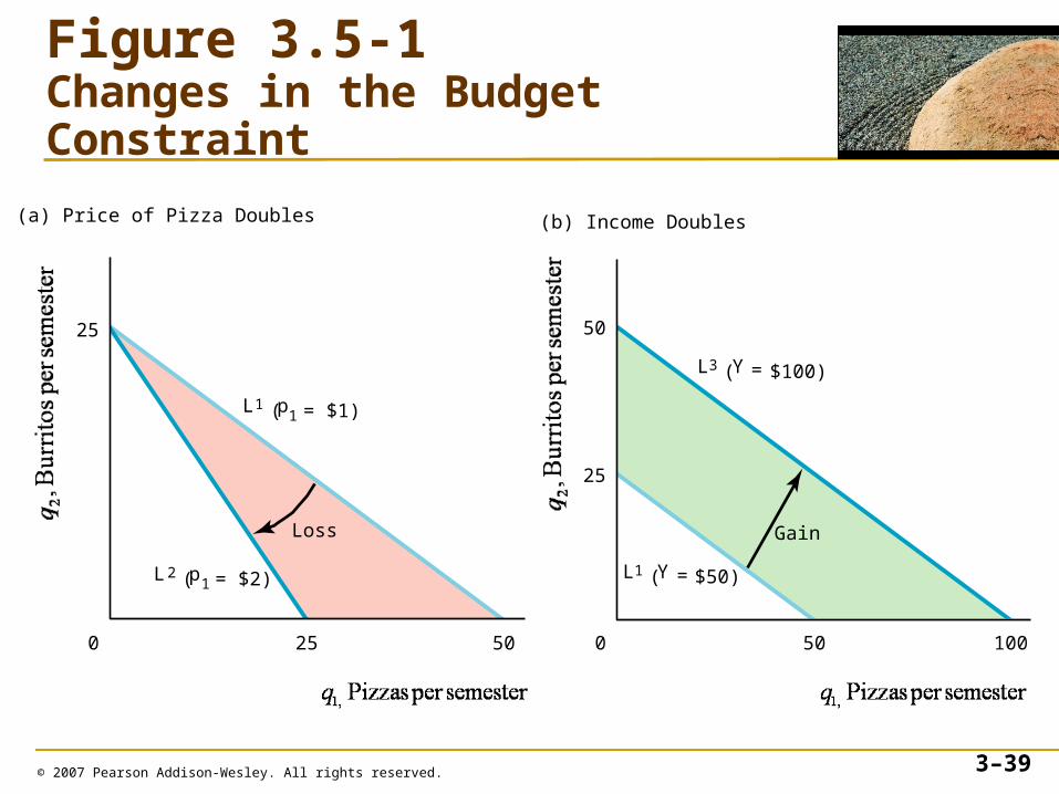
Effect of A Change on Consumption
• If the price of pizza doubles but the price of
burritos is unchanged, the budget constraint
swings in toward the origin in panel a of Figure
3.5-1.
• If the consumer’s income increases, the
consumer can buy more of all goods. The
budget constraint shifts outward—away from
the origin—and is parallel to the origin
constraint in panel b of Figure 3.5-1.
© 2007 Pearson Addison-Wesley. All rights reserved. 3–39
Figure 3.5-1 Changes in the Budget Constraint
(a) Price of Pizza Doubles
Loss
50
L1 (p1 = $1)
L 2 (p1 = $2)
25
250
(b) Income Doubles
Gain
100
L3 (Y = $100)
L1 (Y = $50)
50
25
500
© 2007 Pearson Addison-Wesley. All rights reserved. 3–40
Effect of a Change on Consumption
• A change in income affects only the position and not the slope of the budget line.
• The slope is determined solely by the relative prices of pizza and burritos.
© 2007 Pearson Addison-Wesley. All rights reserved. 3–41
The Consumer’s Optimal Bundle
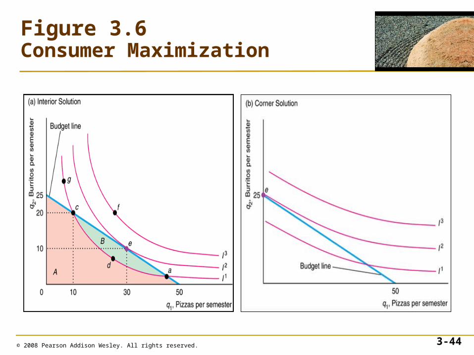
• Bundles that lie on indifference curves above the constraint, such as those on I3, are not in the opportunity set.
• For any bundle inside the constraint (such as d on I1), there is another bundle on the constraint with more of at least one of the two goods, and hence she prefers that bundle.
• Therefore, the optimal bundle must lie on the budget constraint.
© 2007 Pearson Addison-Wesley. All rights reserved. 3–42
The Consumer’s Optimal Bundle
• Bundles that lie on indifference curves that cross
the budget constraint (such as I1, which crosses the constraint at a and c ) are less desirable
than certain other bundles on the constraint.
• Thus the optimal bundle must lie on the budget
constraint and be on an indifference curve that
does not cross it. Such a bundle is the
consumer’s optimum.
The Consumer’s Optimal Bundle
• The optimal bundle must lie on an indifference
curve that touches the budget constraint
but does not cross it.
© 2008 Pearson Addison Wesley. All rights reserved. 3-43
© 2008 Pearson Addison Wesley. All rights reserved. 3-44
Figure 3.6Consumer Maximization
© 2007 Pearson Addison-Wesley. All rights reserved. 3–45
Interior Solution
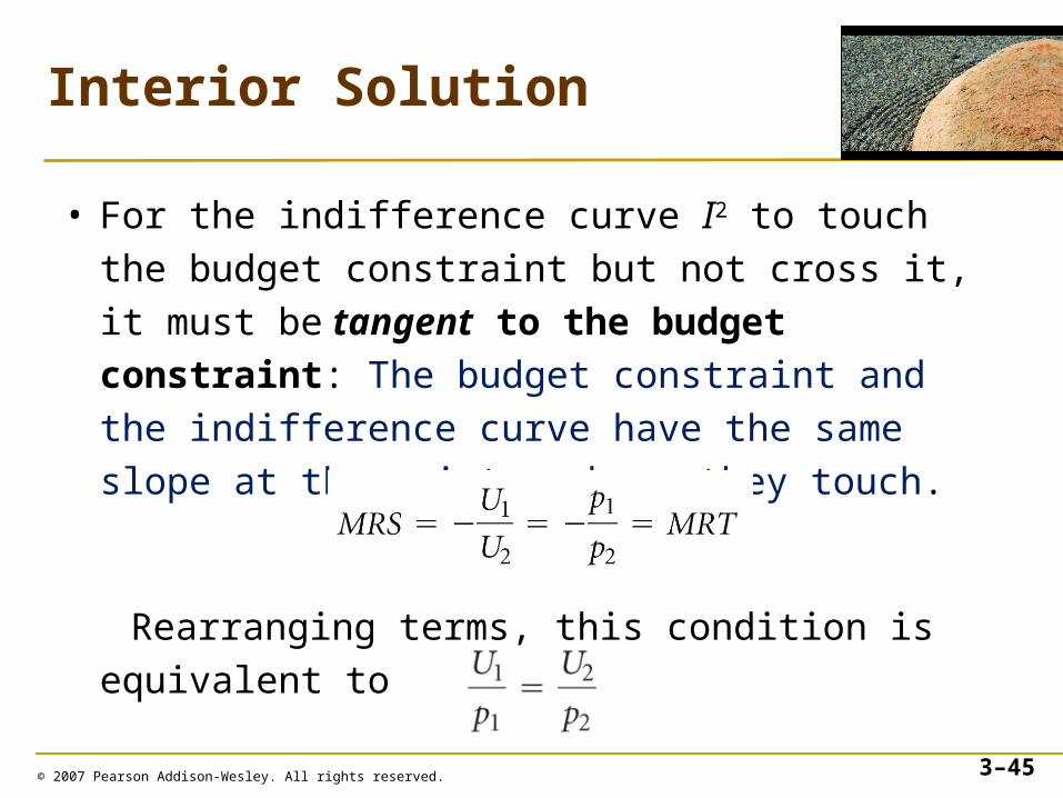
• For the indifference curve I2 to touch the budget
constraint but not cross it, it must be tangent to
the budget constraint: The budget constraint
and the indifference curve have the same slope
at the point e where they touch.
Rearranging terms, this condition is equivalent to
Corner Solution
• There are two ways for an optimal bundle to lie
on an indifference curve that touches the budget
constraint but does not cross it. The first is an
interior solution. The other possibility is called a
corner solution.
– Indifference curve does not cross the constraint into
the opportunity set
– Indifference curve is not tangent to the budget line.
© 2008 Pearson Addison Wesley. All rights reserved. 3-46
© 2008 Pearson Addison Wesley. All rights reserved. 3-47
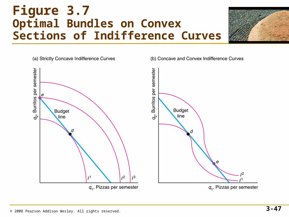
Figure 3.7Optimal Bundles on Convex Sections of Indifference Curves
© 2007 Pearson Addison-Wesley. All rights reserved. 3–48
Buying Where More is Better
• If both goods are consumed in positive quantities and their prices are positive, more of either good must be preferred to less.
• In summary, we do not observe consumer optima at bundles where indifference curves are concave or consumers are satiated. Thus we can safely assume that indifference curves are convex and that consumers prefer more to less in the ranges of goods that we actually observe.
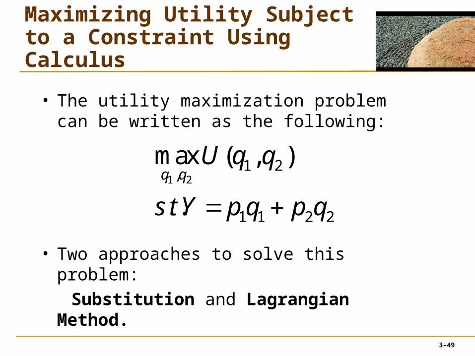
Maximizing Utility Subject to a Constraint Using Calculus
• The utility maximization problem can be written as the following:
• Two approaches to solve this problem:
Substitution and Lagrangian Method.
1 21 2
,max ( , )q qU q q
1 1 2 2. . s t Y p q p q
3–49

Maximizing Utility Subject to a Constraint Using Calculus
• Substitution:
We can substitute the budget constraint into the utility function.
• So we can use standard maximization techniques to solve it.
2
2 22
1
max , q
Y p qU q
p
1 2 21 2
2 1 2 2 1 1 2 1
0
q p pdU U U U UU U
dq q q q p q q p
3–50
Maximizing Utility Subject to a Constraint Using Calculus
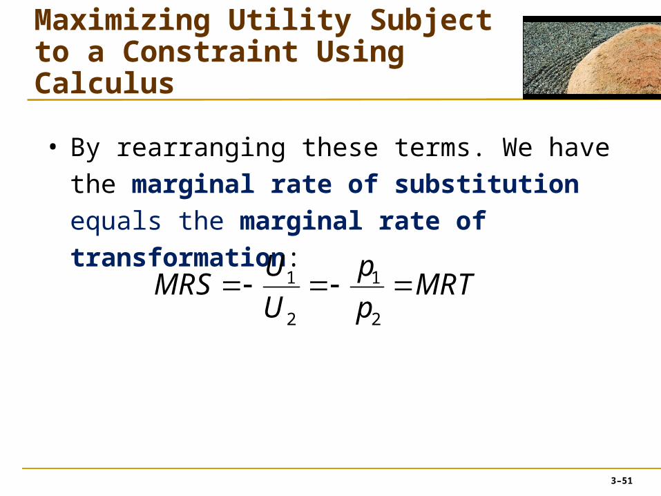
• By rearranging these terms. We have the
marginal rate of substitution equals the
marginal rate of transformation:
1 1
2 2
U p
MRS MRTU p
3–51

Maximizing Utility Subject to a Constraint Using Calculus
• Lagrangian Method:
We write the equivalent Lagrangian problem as
where is the Lagrange multiplier.
© 2008 Pearson Addison Wesley. All rights reserved. 3-52
Maximizing Utility Subject to a Constraint Using Calculus
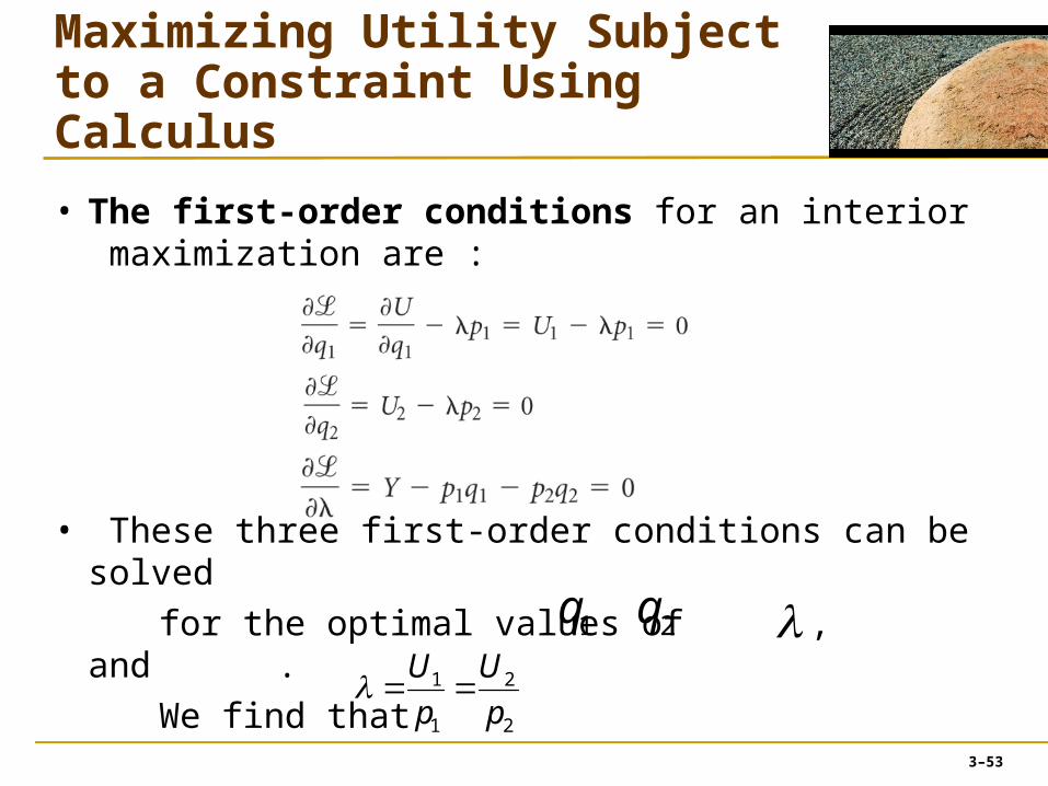
• The first-order conditions for an interior maximization are :
• These three first-order conditions can be solved
for the optimal values of , and .
We find that 1 2
1 2
U U
p p
1q 2q
3–53
Maximizing Utility Subject to a Constraint Using Calculus
• This optimality condition is the same as the
one that we derived using the substitution
method or a graphical approach.
3–54
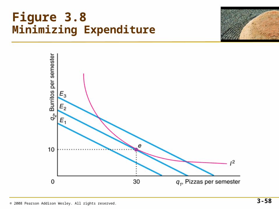
Minimizing Expenditure
• Consider the alternative problem where we ask how Lisa can make the lowest possible expenditure to maintain her utility at a particular level, ,which corresponds to indifference curve .
• The rule for minimizing expenditure while achieving a given level of utility is to choose the lowest expenditure such that the budget line touches — is tangent to — the relevant indifference curve.
U
3–55
2I
Minimizing Expenditure
• Thus solving either of the two problems –
maximizing utility subject to a budget
constraint or minimizing expenditure subject
to maintaining a given level of utility – yields
the same optimal values.
3–56
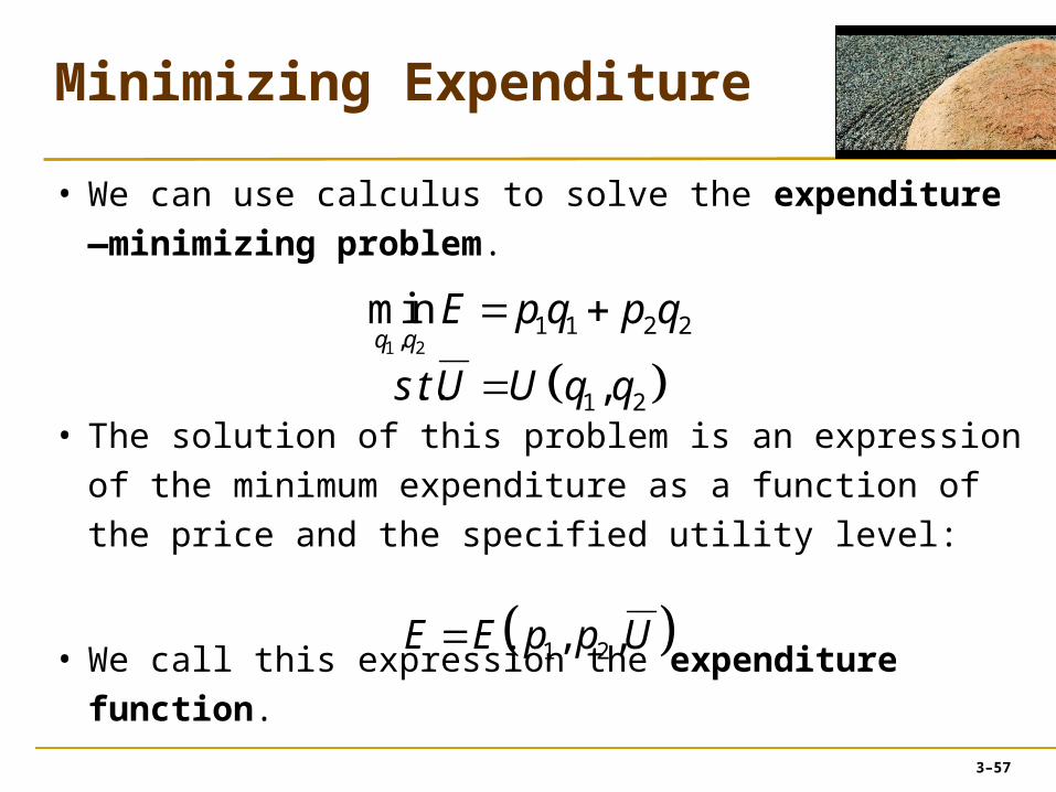
Minimizing Expenditure
• We can use calculus to solve the expenditure —
minimizing problem.
• The solution of this problem is an expression of the
minimum expenditure as a function of the price and
the specified utility level:
• We call this expression the expenditure function.
1 2, ,E E p p U
3–57
1 21 1 2 2
,min q q
E p q p q
1 2. . ,s tU U q q
© 2008 Pearson Addison Wesley. All rights reserved. 3-58
Figure 3.8Minimizing Expenditure