Embed Size (px)
Citation preview

Bézier Splines
陈仁杰
中国科学技术大学
计算机辅助几何设计2021秋学期
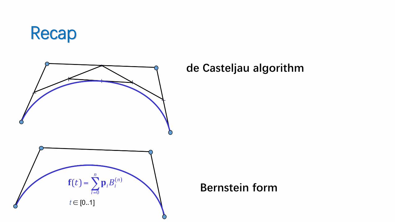
Recap
de Casteljau algorithm
Bernstein form
Recap
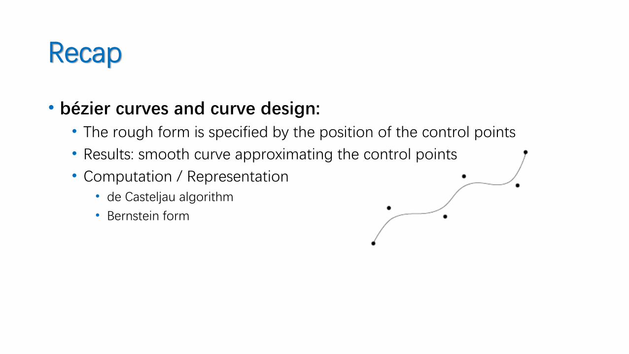
• bézier curves and curve design:• The rough form is specified by the position of the control points
• Results: smooth curve approximating the control points
• Computation / Representation• de Casteljau algorithm
• Bernstein form
Recap
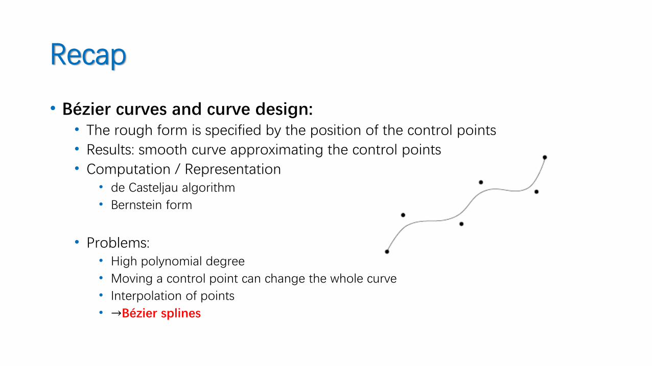
• Bézier curves and curve design:• The rough form is specified by the position of the control points
• Results: smooth curve approximating the control points
• Computation / Representation• de Casteljau algorithm
• Bernstein form
• Problems:• High polynomial degree
• Moving a control point can change the whole curve
• Interpolation of points
• →Bézier splines
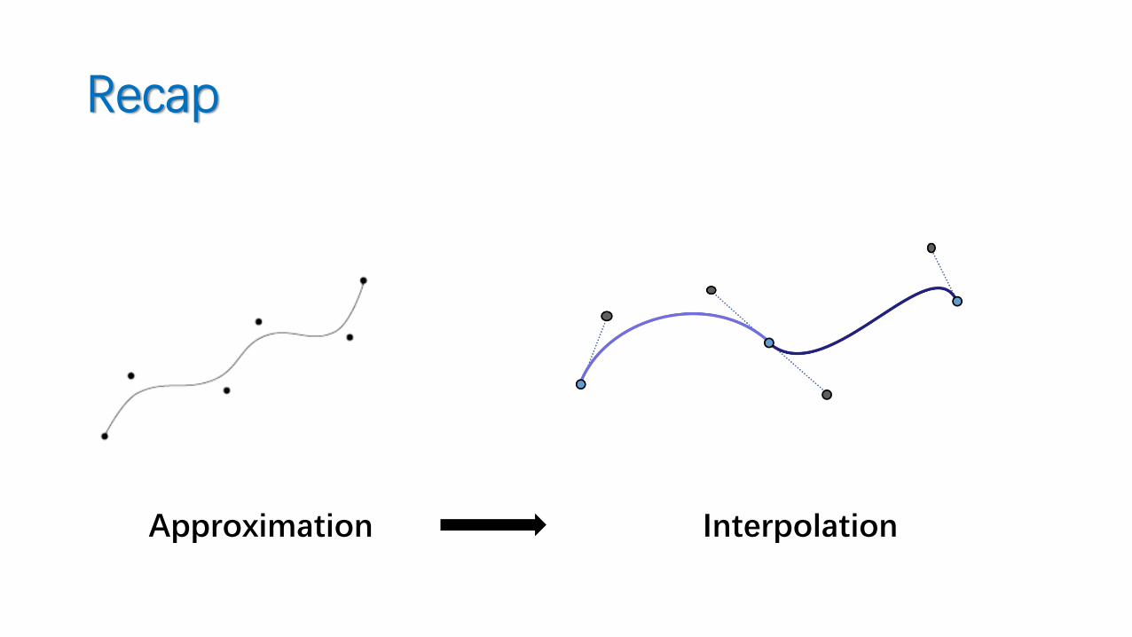
Recap
Approximation Interpolation
Towards Bézier Splines
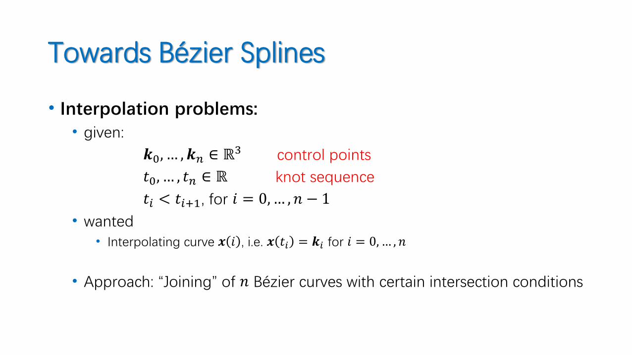
• Interpolation problems:• given:
𝒌0, … , 𝒌𝑛 ∈ ℝ3 control points
𝑡0, … , 𝑡𝑛 ∈ ℝ knot sequence
𝑡𝑖 < 𝑡𝑖+1, for 𝑖 = 0,… , 𝑛 − 1
• wanted• Interpolating curve 𝒙 𝑖 , i.e. 𝒙 𝑡𝑖 = 𝒌𝑖 for 𝑖 = 0, … , 𝑛
• Approach: “Joining” of 𝑛 Bézier curves with certain intersection conditions
Towards Bézier Splines
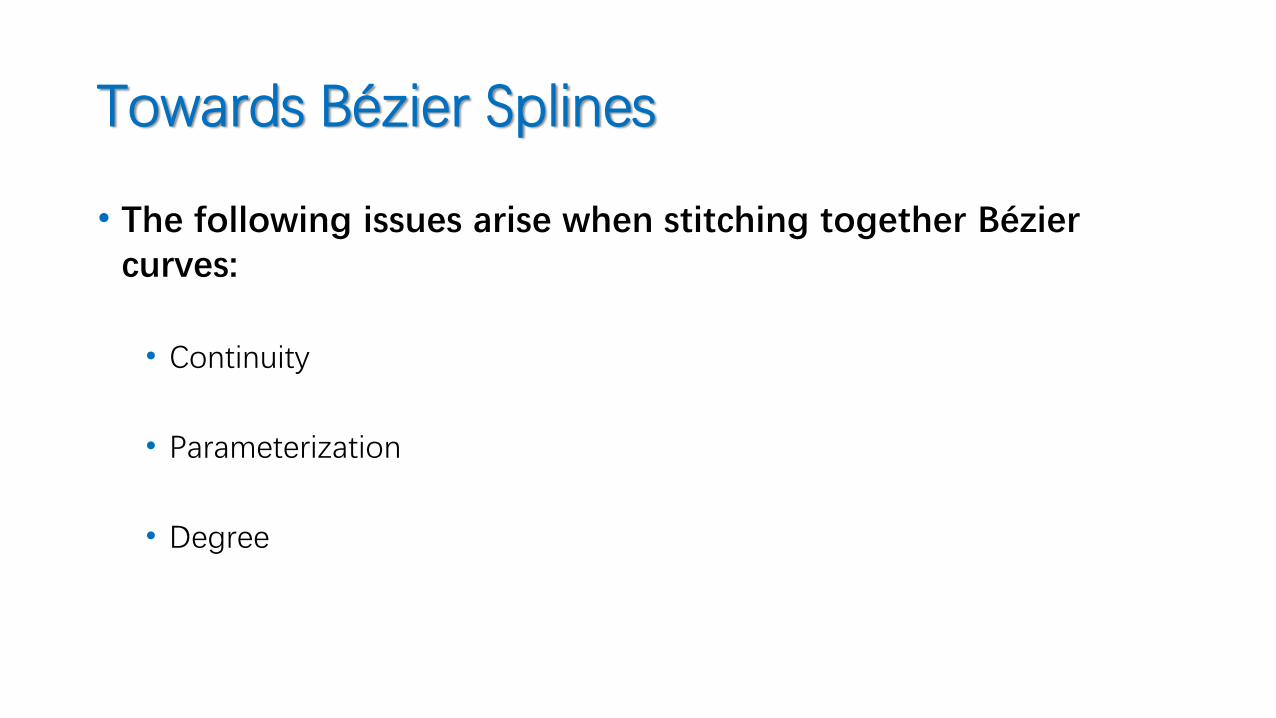
• The following issues arise when stitching together Béziercurves:
• Continuity
• Parameterization
• Degree

Bézier SplinesParametric and Geometric Continuity
Parametric Continuity
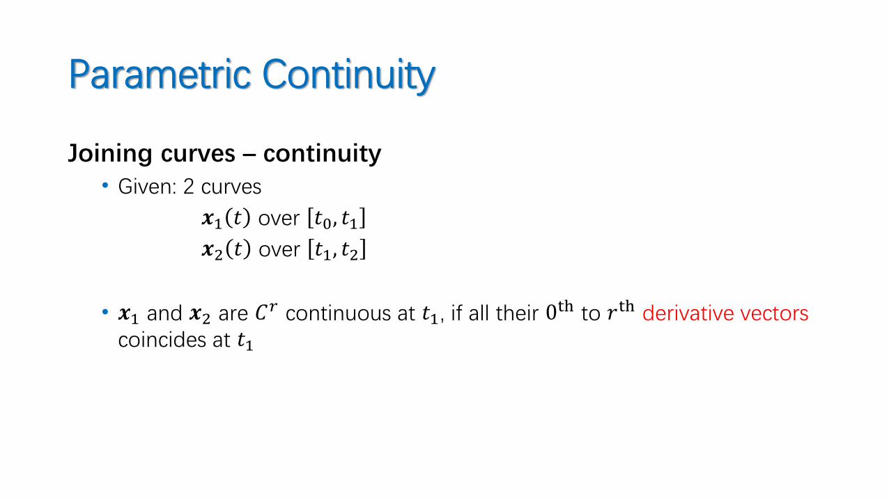
Joining curves – continuity• Given: 2 curves
𝒙1 𝑡 over 𝑡0, 𝑡1𝒙2 𝑡 over 𝑡1, 𝑡2
• 𝒙1 and 𝒙2 are 𝐶𝑟 continuous at 𝑡1, if all their 0th to 𝑟th derivative vectors coincides at 𝑡1
Parametric Continuity
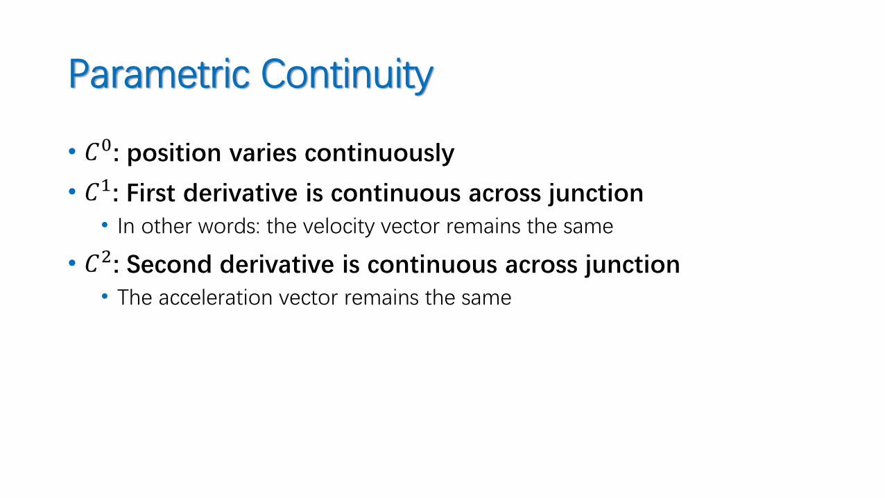
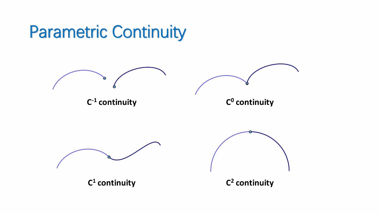
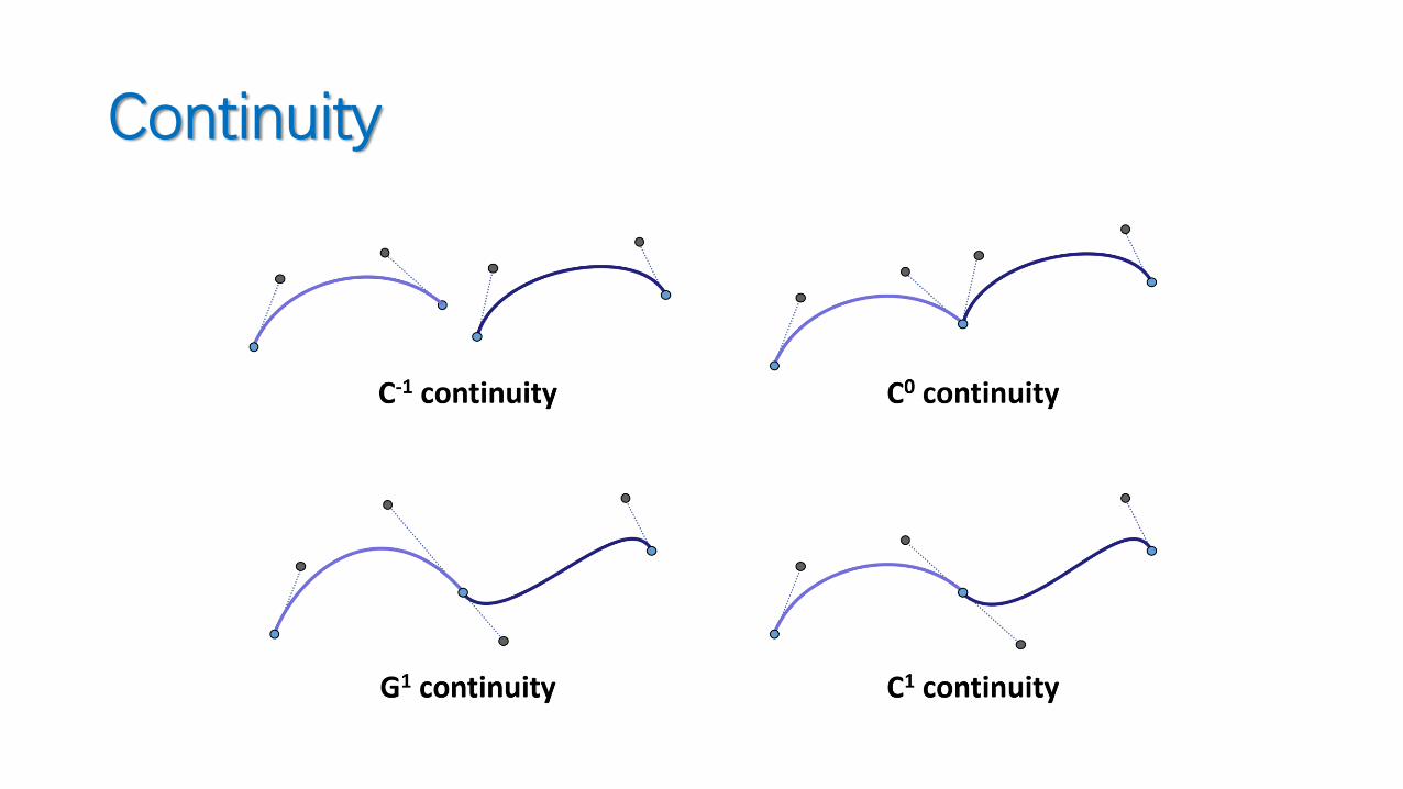
• 𝐶0: position varies continuously
• 𝐶1: First derivative is continuous across junction• In other words: the velocity vector remains the same
• 𝐶2: Second derivative is continuous across junction• The acceleration vector remains the same
Parametric Continuity
Continuity
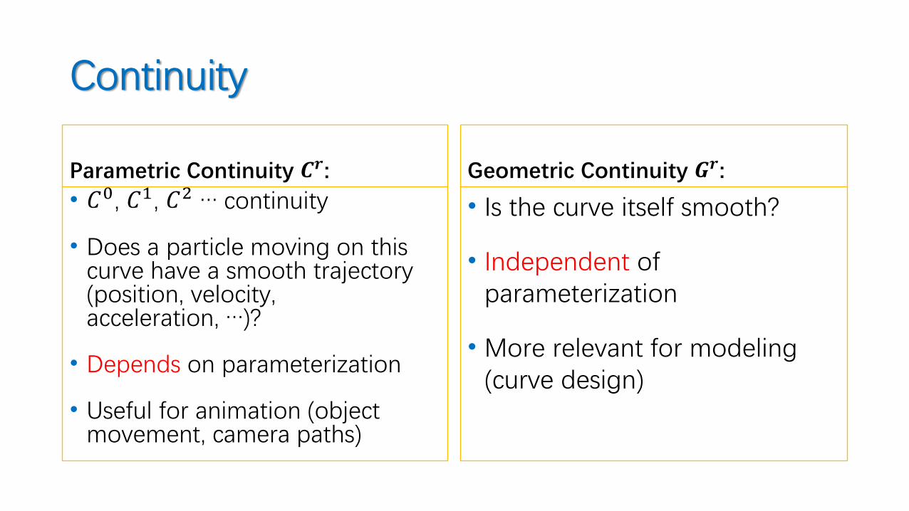
Parametric Continuity 𝑪𝒓:
• 𝐶0, 𝐶1, 𝐶2 … continuity
• Does a particle moving on this curve have a smooth trajectory (position, velocity, acceleration, …)?
• Depends on parameterization
• Useful for animation (object movement, camera paths)
Geometric Continuity 𝑮𝒓:
• Is the curve itself smooth?
• Independent of parameterization
• More relevant for modeling (curve design)
Geometric continuity:
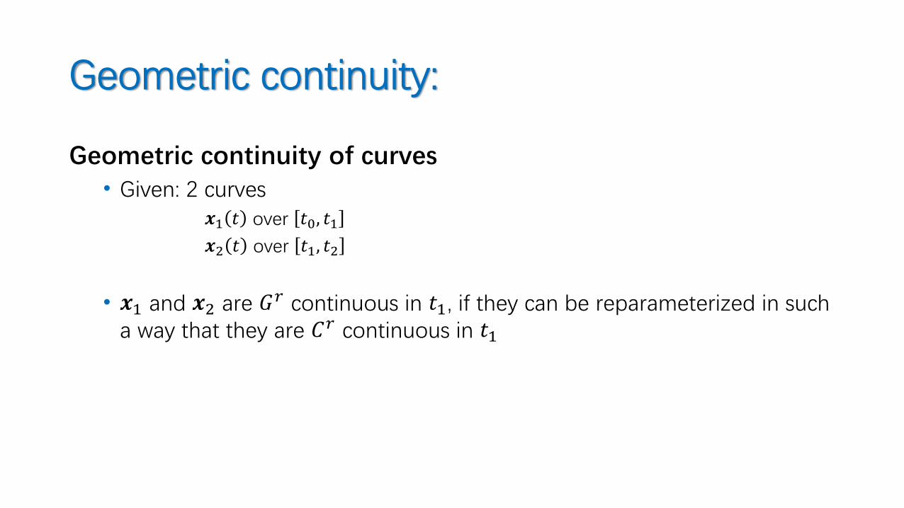
Geometric continuity of curves• Given: 2 curves
𝒙1 𝑡 over 𝑡0, 𝑡1𝒙2 𝑡 over 𝑡1, 𝑡2
• 𝒙1 and 𝒙2 are 𝐺𝑟 continuous in 𝑡1, if they can be reparameterized in such a way that they are 𝐶𝑟 continuous in 𝑡1
Geometric continuity:
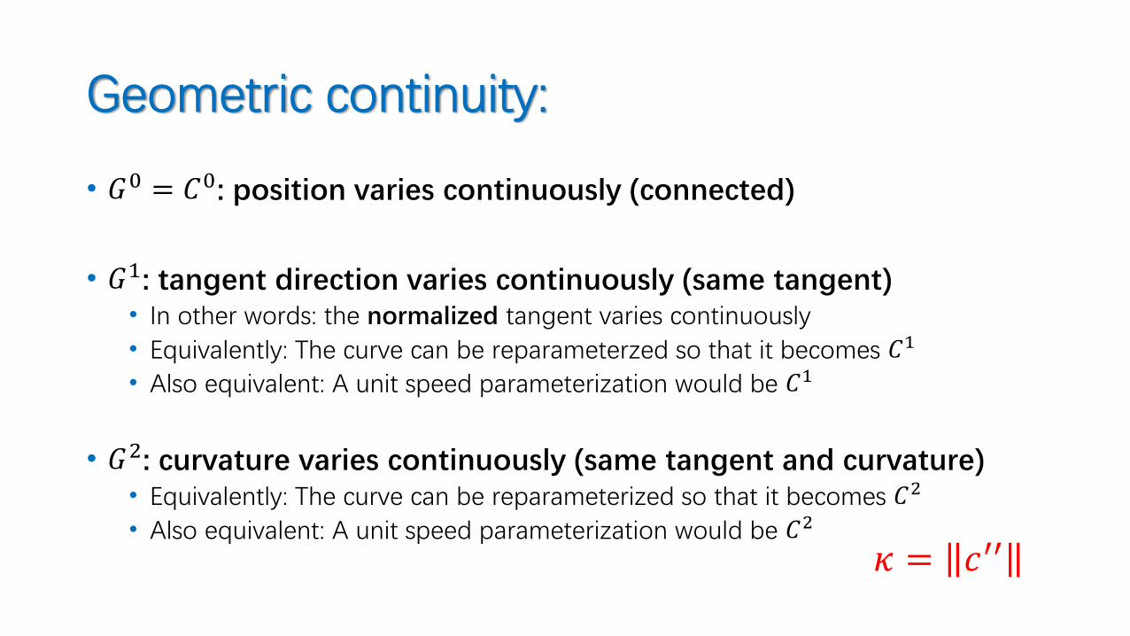
• 𝐺0 = 𝐶0: position varies continuously (connected)
• 𝐺1: tangent direction varies continuously (same tangent)• In other words: the normalized tangent varies continuously
• Equivalently: The curve can be reparameterzed so that it becomes 𝐶1
• Also equivalent: A unit speed parameterization would be 𝐶1
• 𝐺2: curvature varies continuously (same tangent and curvature)• Equivalently: The curve can be reparameterized so that it becomes 𝐶2
• Also equivalent: A unit speed parameterization would be 𝐶2
𝜅 = 𝑐′′

Bézier SplinesParameterization
Bézier spline curves
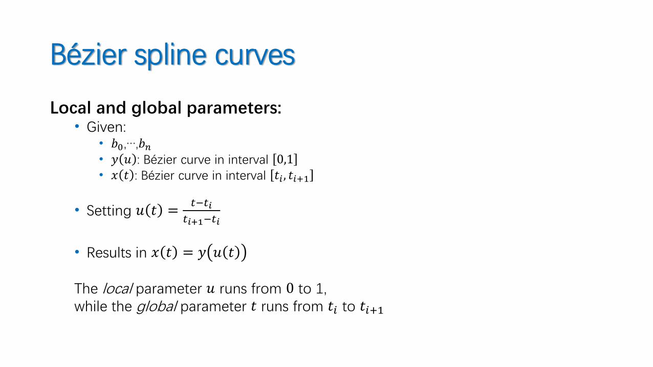
Local and global parameters:• Given:
• 𝑏0,…,𝑏𝑛• 𝑦 𝑢 : Bézier curve in interval 0,1• 𝑥 𝑡 : Bézier curve in interval 𝑡𝑖 , 𝑡𝑖+1
• Setting 𝑢 𝑡 =𝑡−𝑡𝑖
𝑡𝑖+1−𝑡𝑖
• Results in 𝑥 𝑡 = 𝑦 𝑢 𝑡
The local parameter 𝑢 runs from 0 to 1,while the global parameter 𝑡 runs from 𝑡𝑖 to 𝑡𝑖+1
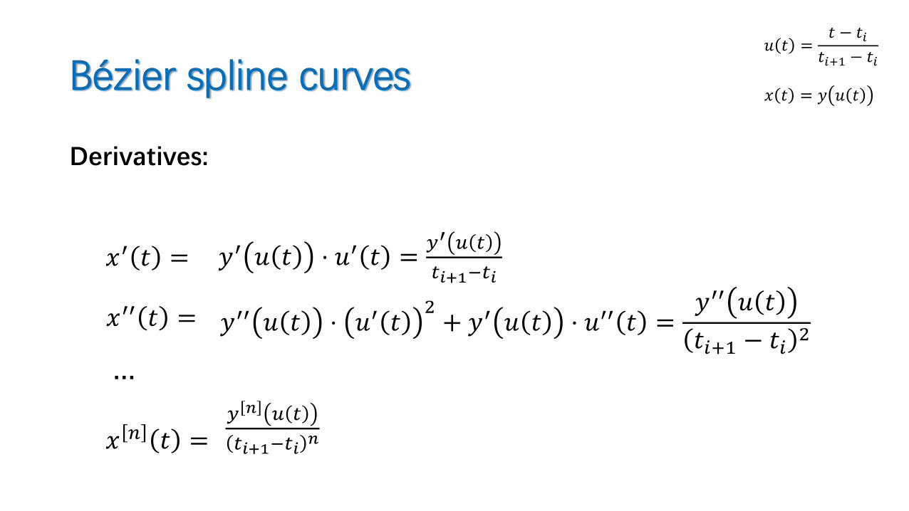
Bézier spline curves
Derivatives:
𝑥′ 𝑡 =
𝑥′′ 𝑡 =
…
𝑥 𝑛 𝑡 =
𝑢 𝑡 =𝑡 − 𝑡𝑖
𝑡𝑖+1 − 𝑡𝑖
𝑥 𝑡 = 𝑦 𝑢 𝑡
𝑦′ 𝑢 𝑡 ⋅ 𝑢′ 𝑡 =𝑦′ 𝑢 𝑡
𝑡𝑖+1−𝑡𝑖
𝑦′′ 𝑢 𝑡 ⋅ 𝑢′ 𝑡2+ 𝑦′ 𝑢 𝑡 ⋅ 𝑢′′ 𝑡 =
𝑦′′ 𝑢 𝑡
𝑡𝑖+1 − 𝑡𝑖2
𝑦 𝑛 𝑢 𝑡
𝑡𝑖+1−𝑡𝑖𝑛
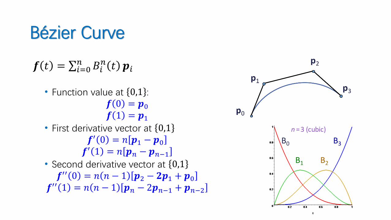
Bézier Curve
𝒇 𝑡 = σ𝑖=0𝑛 𝐵𝑖
𝑛 𝑡 𝒑𝑖
• Function value at 0,1 :𝒇 0 = 𝒑0𝒇 1 = 𝒑1
• First derivative vector at 0,1𝒇′ 0 = 𝑛 𝒑1 − 𝒑0𝒇′ 1 = 𝑛 𝒑𝑛 − 𝒑𝑛−1
• Second derivative vector at 0,1𝒇′′ 0 = 𝑛 𝑛 − 1 𝒑2 − 𝟐𝒑1 + 𝒑0
𝒇′′ 1 = 𝑛 𝑛 − 1 𝒑𝑛 − 2𝒑𝑛−1 + 𝒑𝑛−2
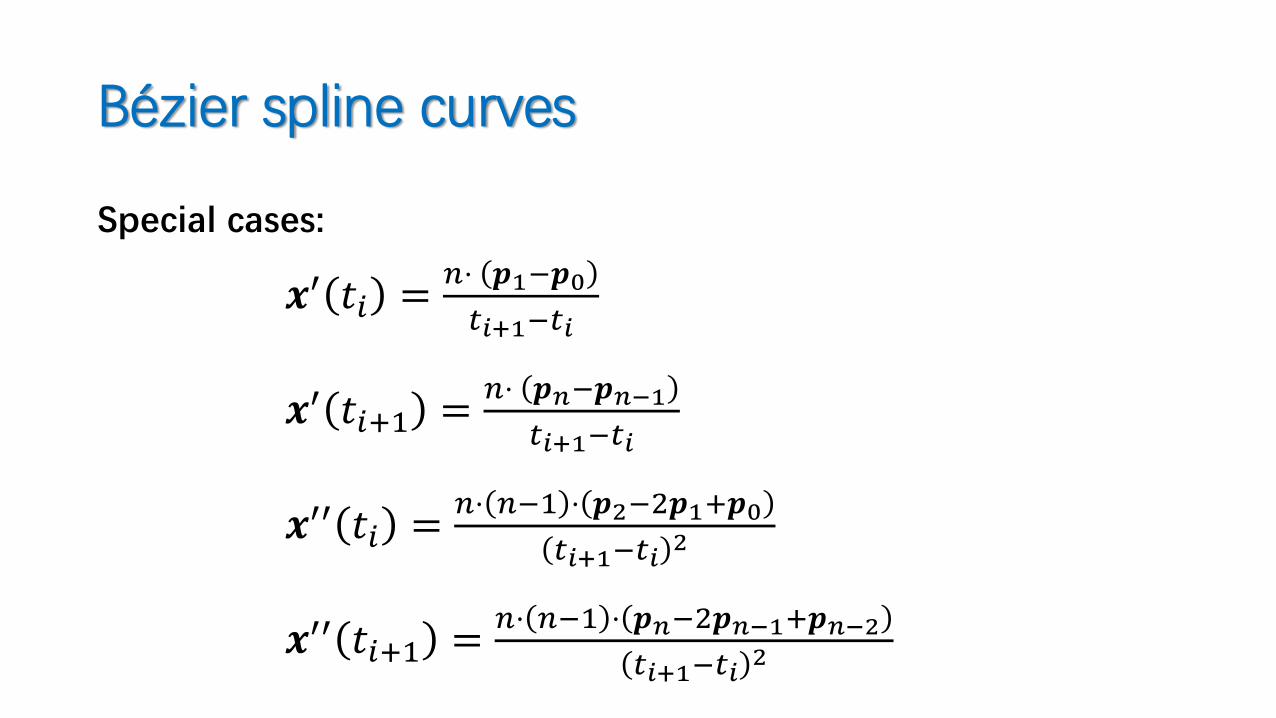
Bézier spline curves
Special cases:
𝒙′ 𝑡𝑖 =𝑛⋅ 𝒑1−𝒑0
𝑡𝑖+1−𝑡𝑖
𝒙′ 𝑡𝑖+1 =𝑛⋅ 𝒑𝑛−𝒑𝑛−1
𝑡𝑖+1−𝑡𝑖
𝒙′′ 𝑡𝑖 =𝑛⋅ 𝑛−1 ⋅ 𝒑2−2𝒑1+𝒑0
𝑡𝑖+1−𝑡𝑖2
𝒙′′ 𝑡𝑖+1 =𝑛⋅ 𝑛−1 ⋅ 𝒑𝑛−2𝒑𝑛−1+𝒑𝑛−2
𝑡𝑖+1−𝑡𝑖2

Bézier SplinesGeneral Case
Bézier spline curves
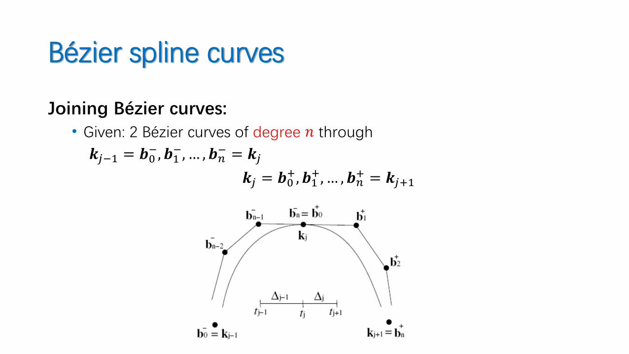
Joining Bézier curves:• Given: 2 Bézier curves of degree 𝑛 through
𝒌𝑗−1 = 𝒃0−, 𝒃1
−, … , 𝒃𝑛− = 𝒌𝑗
𝒌𝑗 = 𝒃0+, 𝒃1
+, … , 𝒃𝑛+ = 𝒌𝑗+1
Bézier spline curves
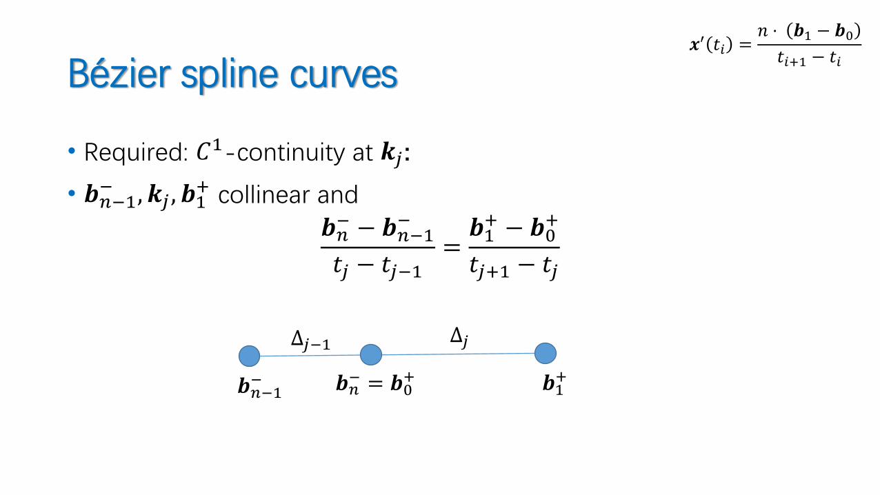
• Required: 𝐶1-continuity at 𝒌𝑗:
• 𝒃𝑛−1− , 𝒌𝑗 , 𝒃1
+ collinear and
𝒃𝑛− − 𝒃𝑛−1
−
𝑡𝑗 − 𝑡𝑗−1=𝒃1+ − 𝒃0
+
𝑡𝑗+1 − 𝑡𝑗
Δ𝑗−1 Δ𝑗
𝒃𝑛− = 𝒃0
+𝒃𝑛−1− 𝒃1
+
𝒙′ 𝑡𝑖 =𝑛 ⋅ 𝒃1 − 𝒃0𝑡𝑖+1 − 𝑡𝑖
Bézier spline curves
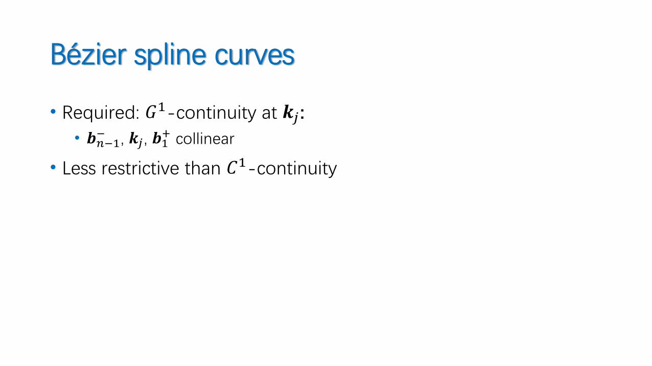
• Required: 𝐺1-continuity at 𝒌𝑗:
• 𝒃𝑛−1− , 𝒌𝑗 , 𝒃1
+ collinear
• Less restrictive than 𝐶1-continuity

Bézier SplinesChoosing the degree
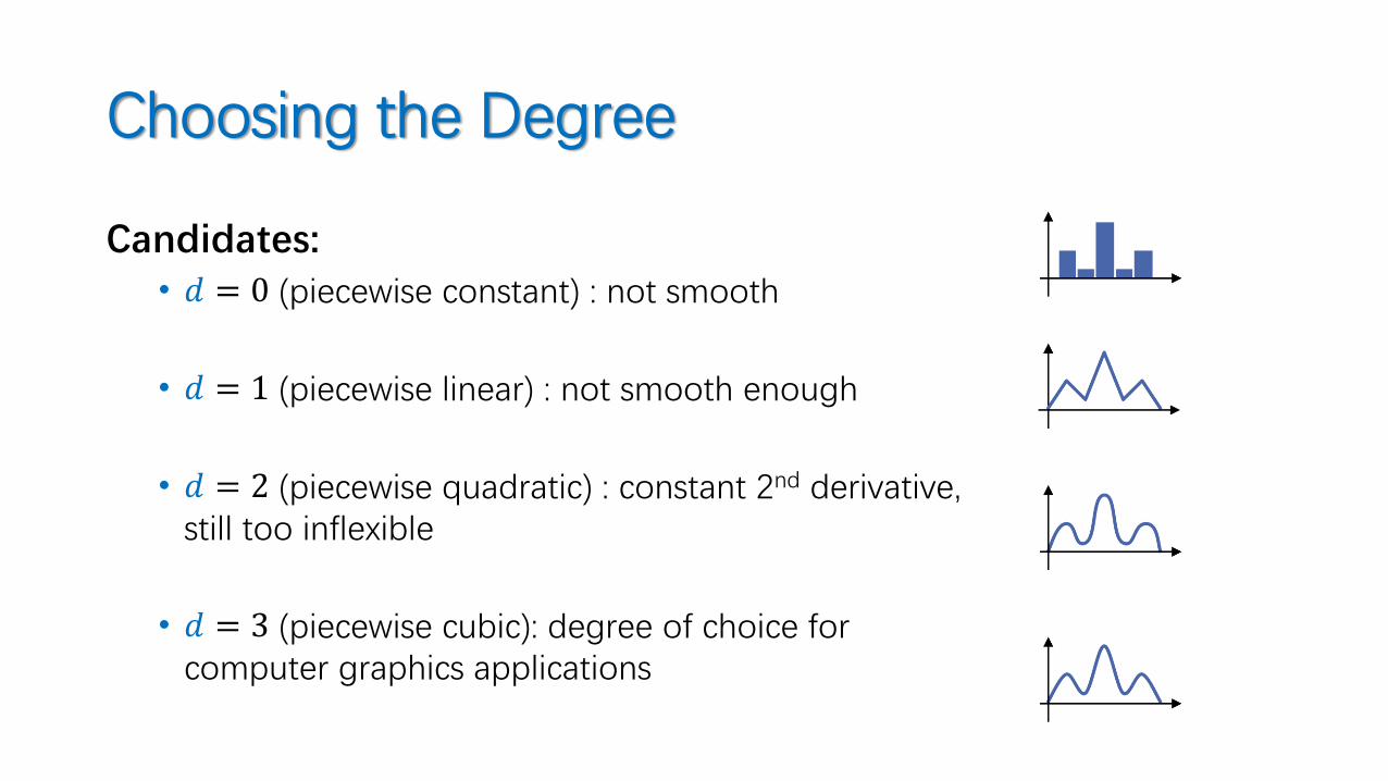
Choosing the Degree
Candidates:• 𝑑 = 0 (piecewise constant) : not smooth
• 𝑑 = 1 (piecewise linear) : not smooth enough
• 𝑑 = 2 (piecewise quadratic) : constant 2nd derivative, still too inflexible
• 𝑑 = 3 (piecewise cubic): degree of choice for computer graphics applications
Cubic Splines
Cubic piecewise polynomials:• We can attain 𝐶2 continuity without fixing the second derivative
throughout the curve
Cubic Splines
Cubic piecewise polynomials:• We can attain 𝐶2 continuity without fixing the second derivative
throughout the curve
• 𝐶2 continuity is perceptually important
• Motion: continuous position, velocity & acceleration
Discontinuous acceleration noticeable (object/camera motion)
• We can see second order shading discontinuities
(esp.: reflective objects)
Cubic Splines
Cubic piecewise polynomials• We can attain 𝐶2 continuity without fixing the second derivative throughout the
curve
• 𝐶2 continuity is perceptually important• We can see second order shading discontinuities
(esp.: reflective objects)
• Motion: continuous position, velocity & accelerationDiscontinuous acceleration noticeable (object/camera motion)
• One more argument for cubics:• Among all 𝐶2 curves that interpolate a set of points (and obey to the same end
condition), a piecewise cubic curve has the least integral acceleration (“smoothest curve you can get”).
Bézier Splines
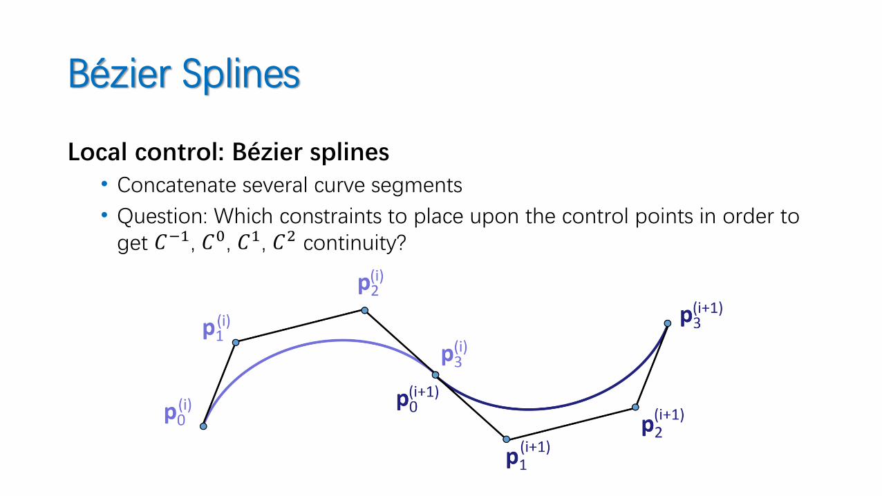
Local control: Bézier splines• Concatenate several curve segments
• Question: Which constraints to place upon the control points in order to get 𝐶−1, 𝐶0, 𝐶1, 𝐶2 continuity?
Bézier Spline Continuity
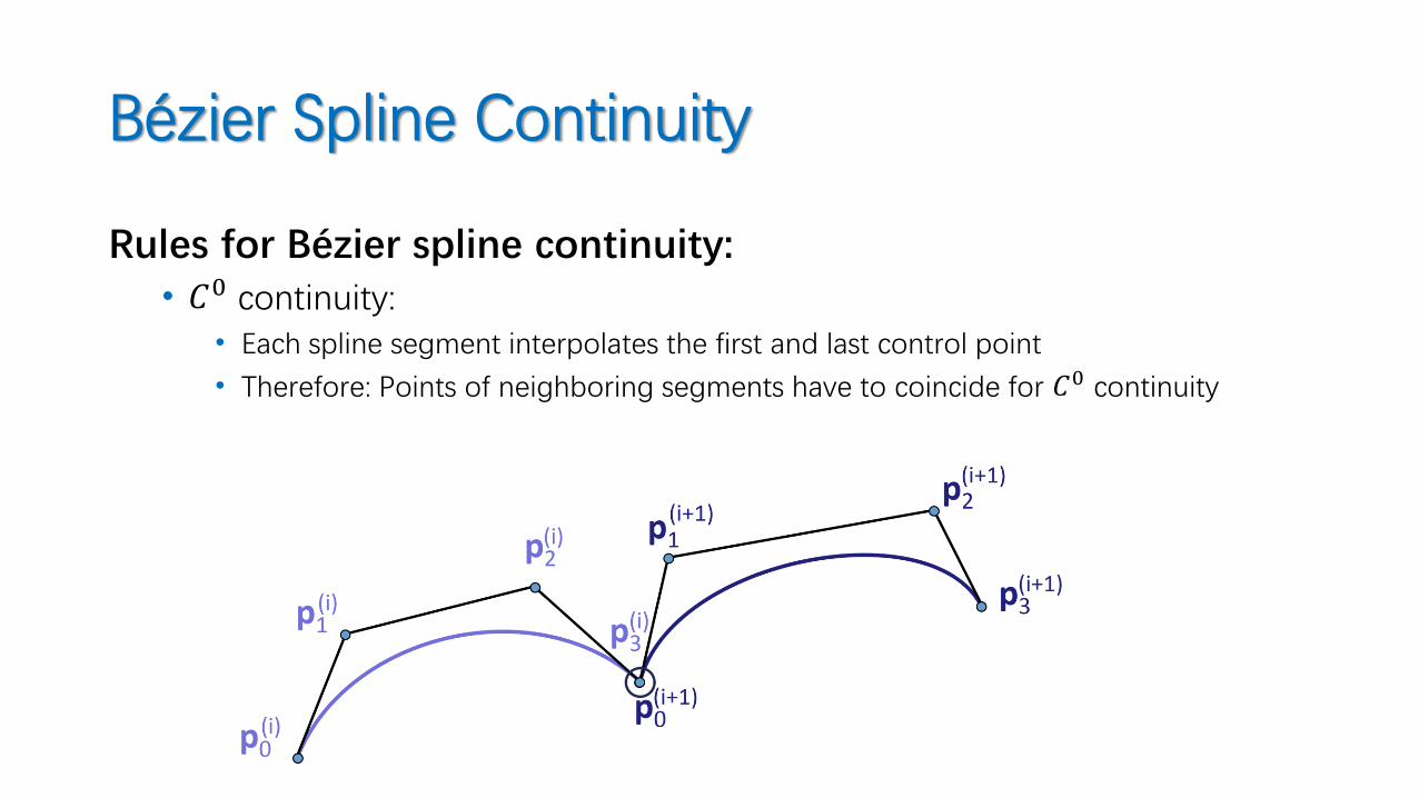
Rules for Bézier spline continuity:• 𝐶0 continuity:
• Each spline segment interpolates the first and last control point
• Therefore: Points of neighboring segments have to coincide for 𝐶0 continuity
Bézier Spline Continuity
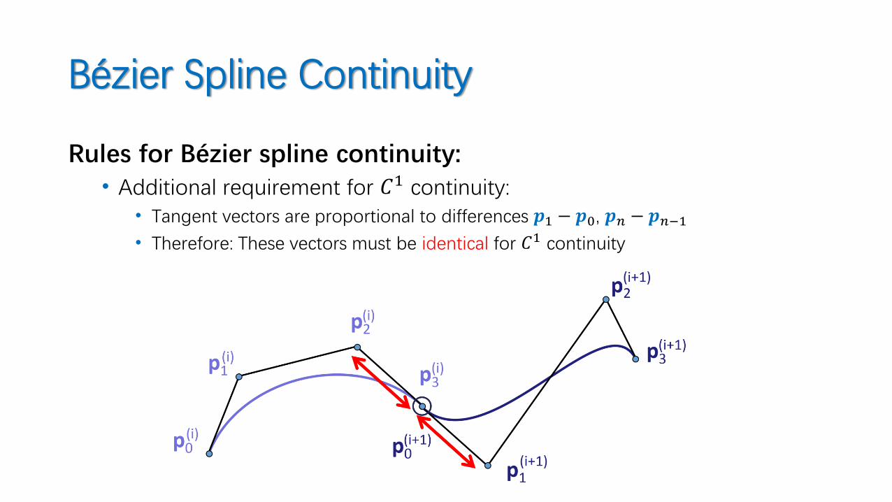
Rules for Bézier spline continuity:• Additional requirement for 𝐶1 continuity:
• Tangent vectors are proportional to differences 𝒑1 − 𝒑0, 𝒑𝑛 − 𝒑𝑛−1
• Therefore: These vectors must be identical for 𝐶1 continuity
Bézier Spline Continuity
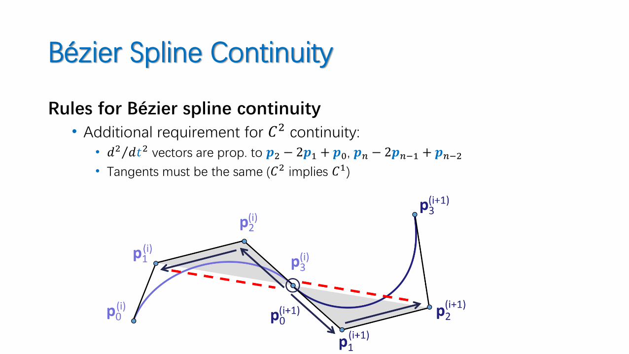
Rules for Bézier spline continuity• Additional requirement for 𝐶2 continuity:
• Τ𝑑2 𝑑𝑡2 vectors are prop. to 𝒑2 − 2𝒑1 + 𝒑0, 𝒑𝑛 − 2𝒑𝑛−1 + 𝒑𝑛−2• Tangents must be the same (𝐶2 implies 𝐶1)
Continuity
Continuity for Bézier Splines
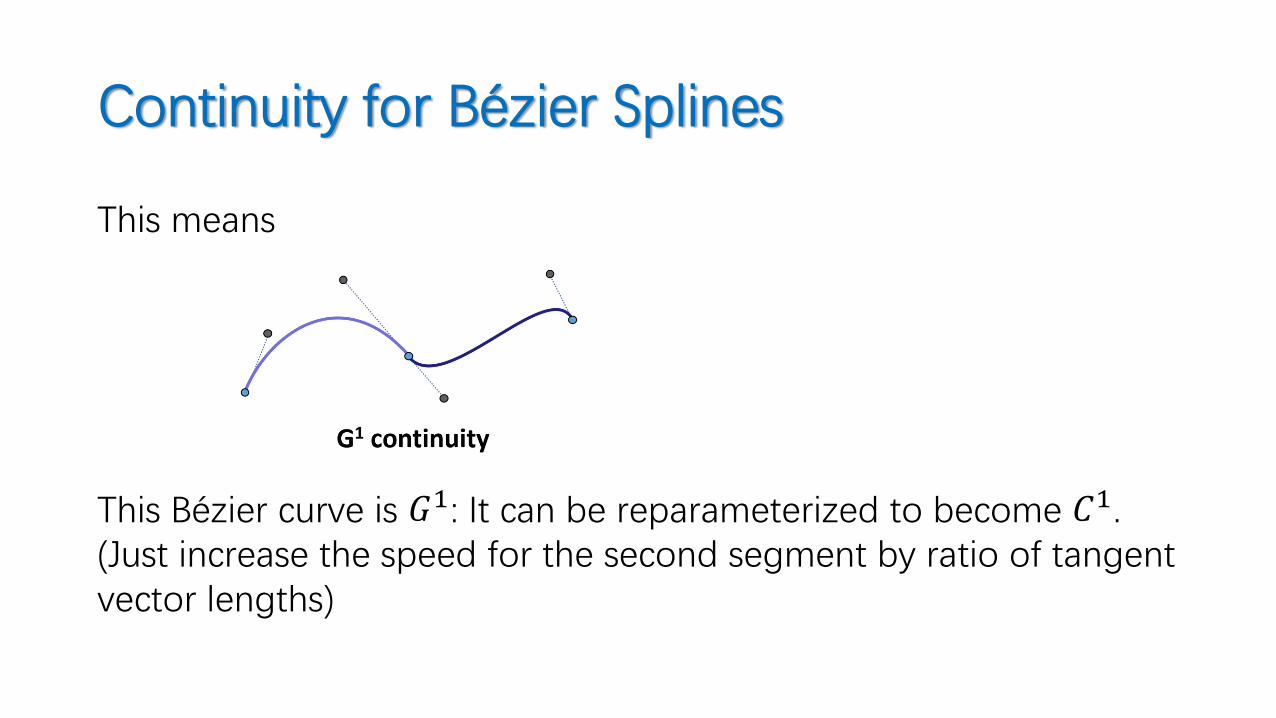
This means
This Bézier curve is 𝐺1: It can be reparameterized to become 𝐶1. (Just increase the speed for the second segment by ratio of tangent vector lengths)
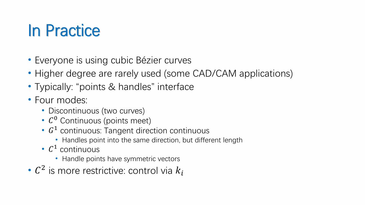
In Practice
• Everyone is using cubic Bézier curves
• Higher degree are rarely used (some CAD/CAM applications)
• Typically: “points & handles” interface
• Four modes:• Discontinuous (two curves)• 𝐶0 Continuous (points meet)• 𝐺1 continuous: Tangent direction continuous
• Handles point into the same direction, but different length
• 𝐶1 continuous• Handle points have symmetric vectors
• 𝐶2 is more restrictive: control via 𝑘𝑖
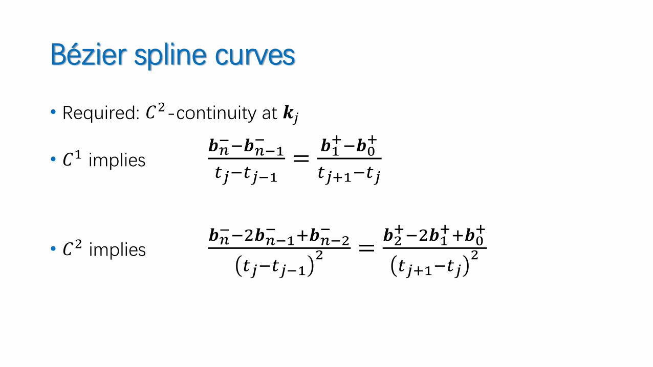
Bézier spline curves
• Required: 𝐶2-continuity at 𝒌𝑗
• 𝐶1 implies 𝒃𝑛−−𝒃𝑛−1
−
𝑡𝑗−𝑡𝑗−1=
𝒃1+−𝒃0
+
𝑡𝑗+1−𝑡𝑗
• 𝐶2 implies 𝒃𝑛−−2𝒃𝑛−1
− +𝒃𝑛−2−
𝑡𝑗−𝑡𝑗−12 =
𝒃2+−2𝒃1
++𝒃0+
𝑡𝑗+1−𝑡𝑗2
Bézier spline curves
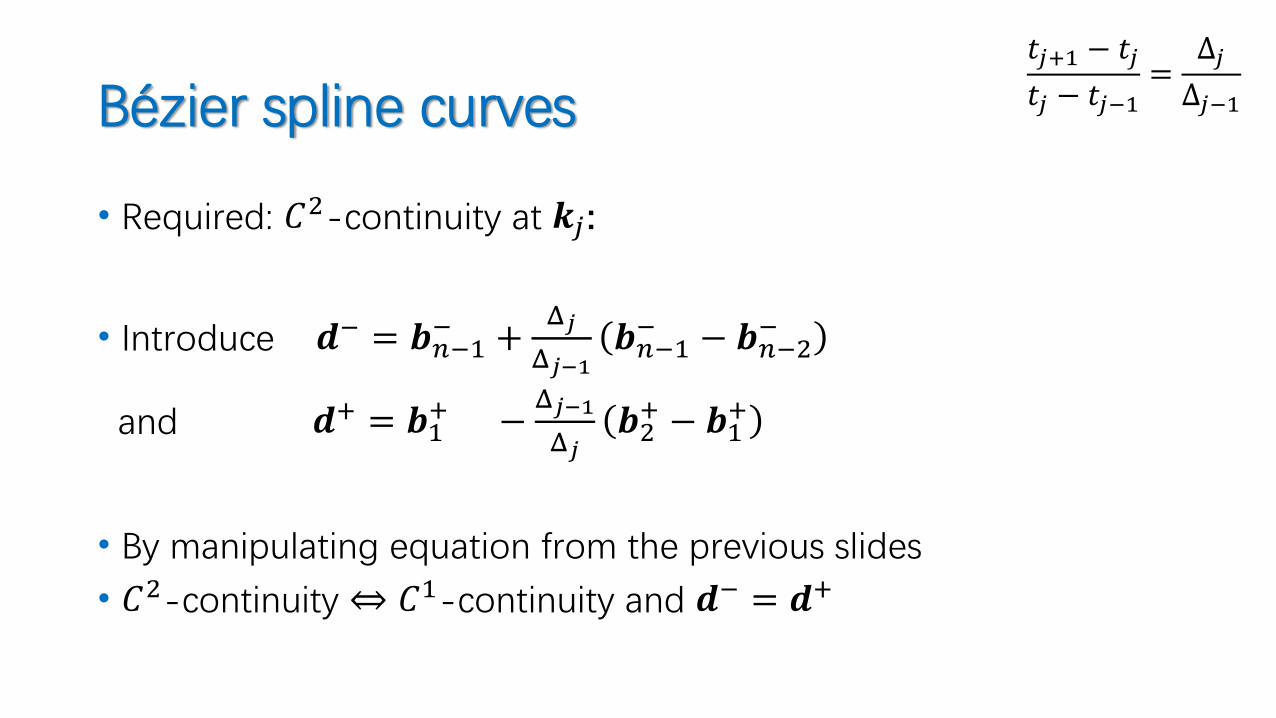
• Required: 𝐶2-continuity at 𝒌𝑗:
• Introduce 𝒅− = 𝒃𝑛−1− +
Δ𝑗
Δ𝑗−1𝒃𝑛−1− − 𝒃𝑛−2
−
and 𝒅+ = 𝒃1+ −
Δ𝑗−1
Δ𝑗𝒃2+ − 𝒃1
+
• By manipulating equation from the previous slides
• 𝐶2-continuity ⇔ 𝐶1-continuity and 𝒅− = 𝒅+
𝑡𝑗+1 − 𝑡𝑗𝑡𝑗 − 𝑡𝑗−1
=Δ𝑗Δ𝑗−1
Bézier spline curves
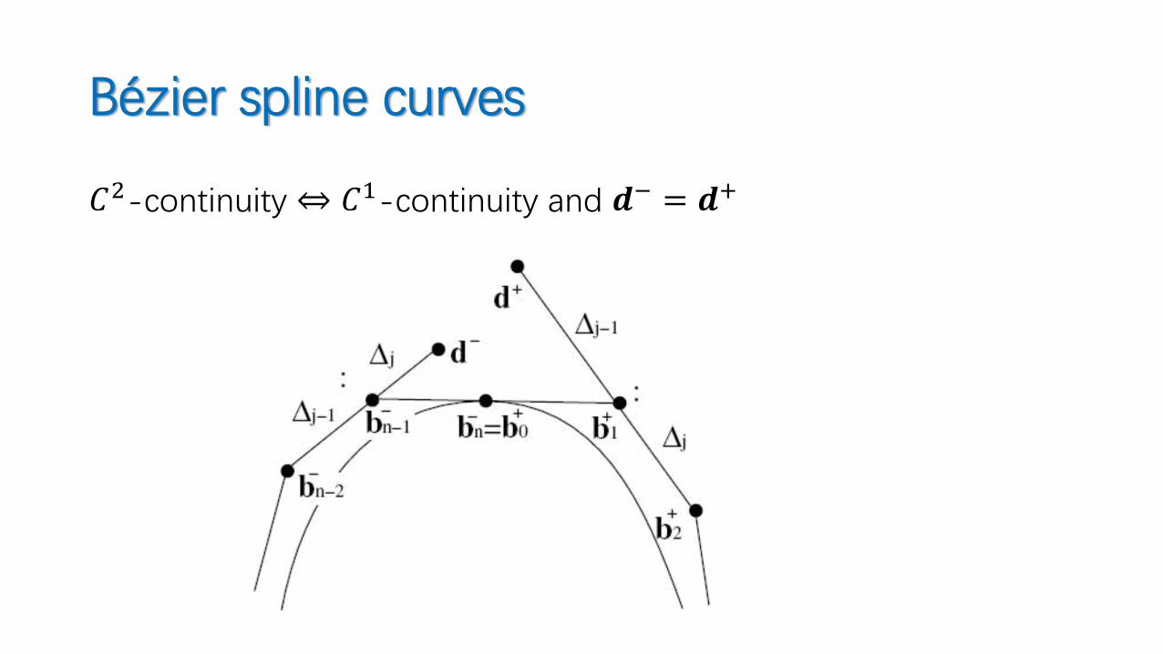
𝐶2-continuity ⇔ 𝐶1-continuity and 𝒅− = 𝒅+
Bézier spline curves
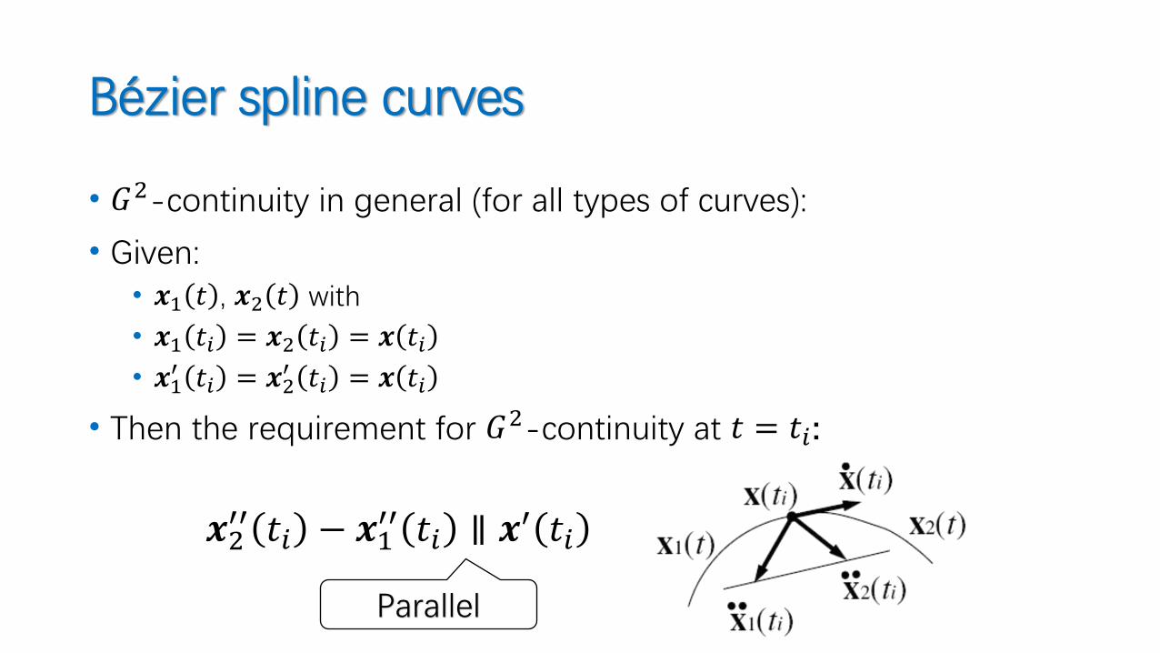
• 𝐺2-continuity in general (for all types of curves):
• Given:• 𝒙1 𝑡 , 𝒙2 𝑡 with
• 𝒙1 𝑡𝑖 = 𝒙2 𝑡𝑖 = 𝒙 𝑡𝑖• 𝒙1
′ 𝑡𝑖 = 𝒙2′ 𝑡𝑖 = 𝒙 𝑡𝑖
• Then the requirement for 𝐺2-continuity at 𝑡 = 𝑡𝑖:
𝒙2′′ 𝑡𝑖 − 𝒙1
′′ 𝑡𝑖 ∥ 𝒙′ 𝑡𝑖
Parallel
Bézier spline curves
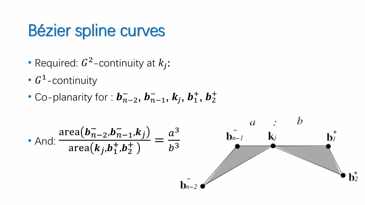
• Required: 𝐺2-continuity at 𝑘𝑗:
• 𝐺1-continuity
• Co-planarity for : 𝒃𝑛−2− , 𝒃𝑛−1
− , 𝒌𝑗, 𝒃1+, 𝒃2
+
• And:area 𝒃𝑛−2
− ,𝒃𝑛−1− ,𝒌𝑗
area 𝒌𝑗,𝒃1+,𝒃2
+ =𝑎3
𝑏3

Bézier Splines𝐶2 Cubic Bézier Splines
Cubic Bézier Splines
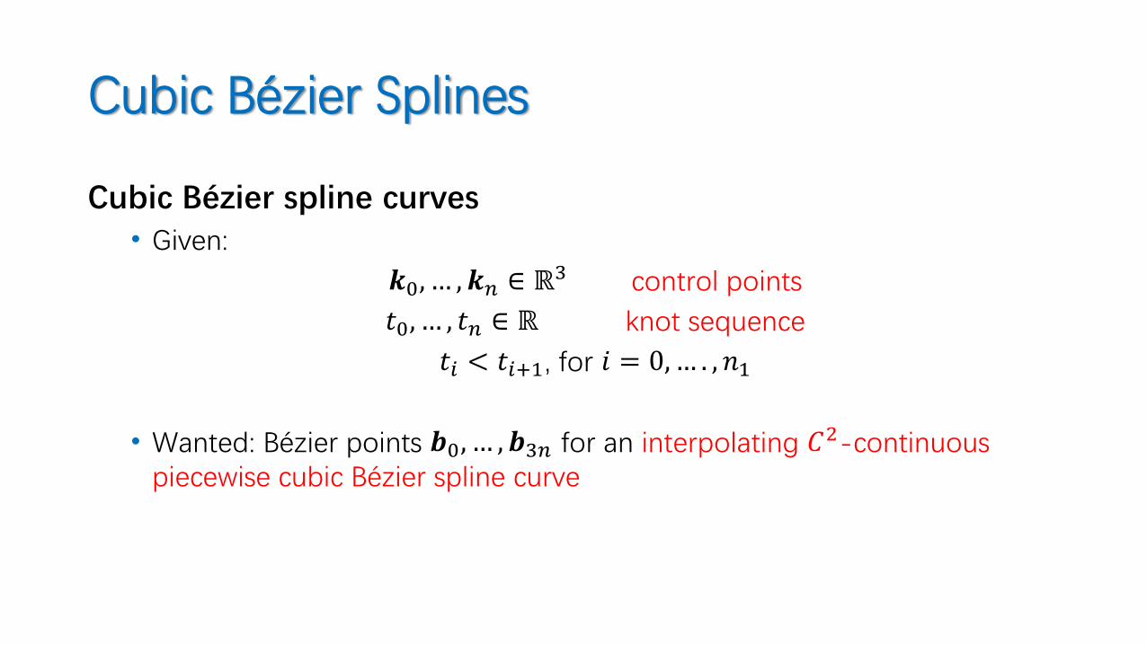
Cubic Bézier spline curves• Given:
𝒌0, … , 𝒌𝑛 ∈ ℝ3 control points
𝑡0, … , 𝑡𝑛 ∈ ℝ knot sequence
𝑡𝑖 < 𝑡𝑖+1, for 𝑖 = 0,… . , 𝑛1
• Wanted: Bézier points 𝒃0, … , 𝒃3𝑛 for an interpolating 𝐶2-continuous piecewise cubic Bézier spline curve

Cubic Bézier Splines
Examples: 𝑛 = 3:
Cubic Bézier Splines
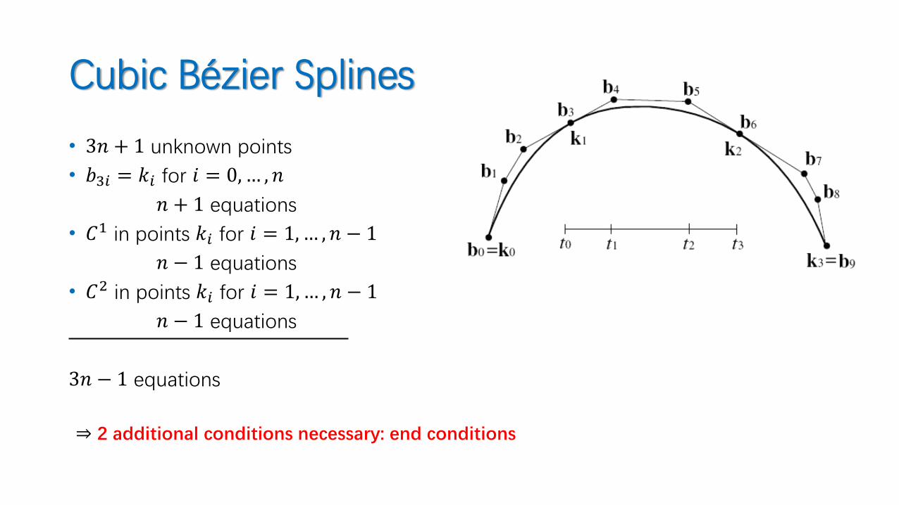
• 3𝑛 + 1 unknown points
• 𝑏3𝑖 = 𝑘𝑖 for 𝑖 = 0,… , 𝑛
𝑛 + 1 equations
• 𝐶1 in points 𝑘𝑖 for 𝑖 = 1, … , 𝑛 − 1
𝑛 − 1 equations
• 𝐶2 in points 𝑘𝑖 for 𝑖 = 1,… , 𝑛 − 1
𝑛 − 1 equations
3𝑛 − 1 equations
⇒ 2 additional conditions necessary: end conditions

Bézier Splines𝐶2 Cubic Bézier Splines: End conditions
Bézier spline curves: End conditions
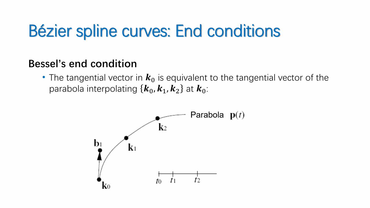
Bessel’s end condition• The tangential vector in 𝒌0 is equivalent to the tangential vector of the
parabola interpolating 𝒌0, 𝒌1, 𝒌2 at 𝒌0:
Bézier spline curves: End conditions
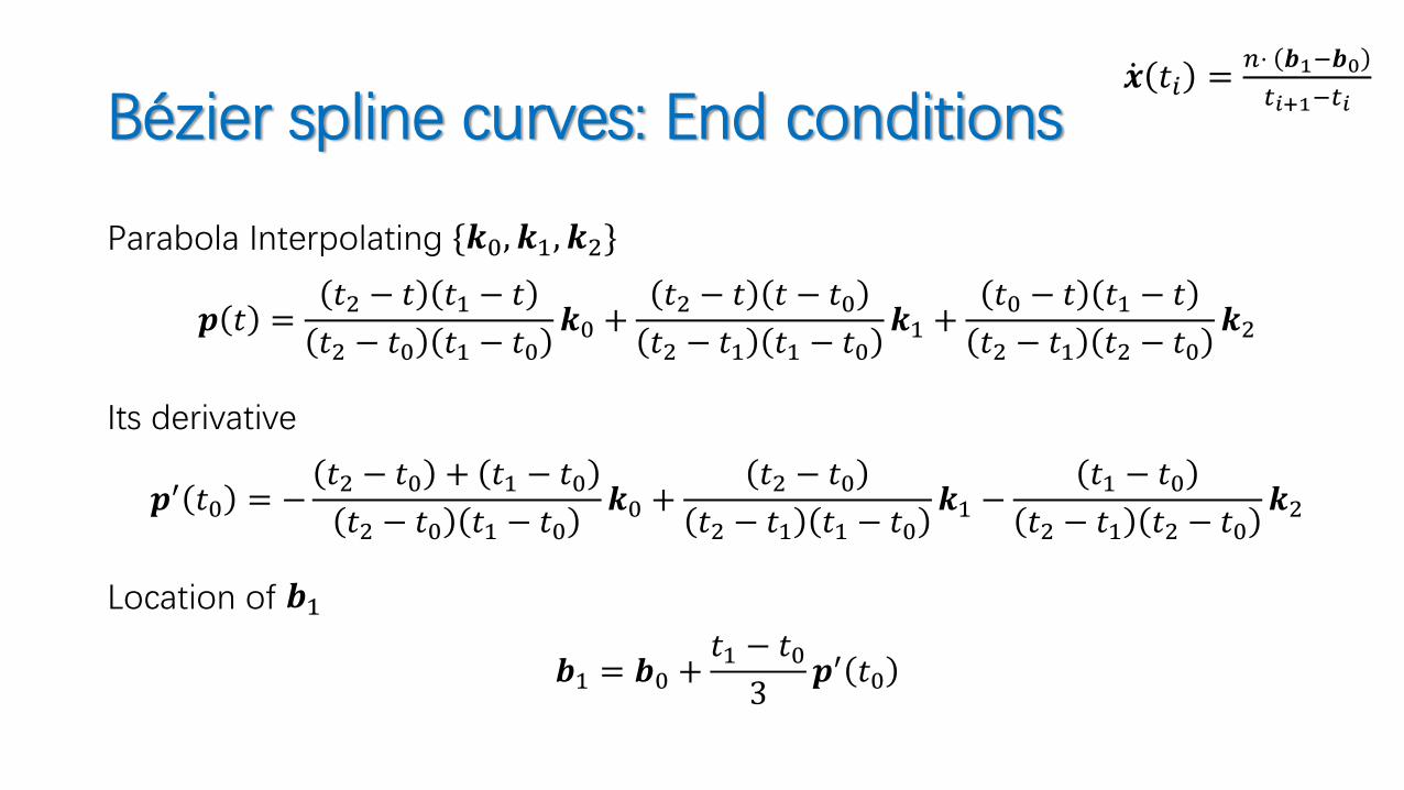
Parabola Interpolating {𝒌0, 𝒌1, 𝒌2}
𝒑 𝑡 =𝑡2 − 𝑡 𝑡1 − 𝑡
𝑡2 − 𝑡0 𝑡1 − 𝑡0𝒌0 +
𝑡2 − 𝑡 𝑡 − 𝑡0𝑡2 − 𝑡1 𝑡1 − 𝑡0
𝒌1 +𝑡0 − 𝑡 𝑡1 − 𝑡
𝑡2 − 𝑡1 𝑡2 − 𝑡0𝒌2
Its derivative
𝒑′ 𝑡0 = −𝑡2 − 𝑡0 + 𝑡1 − 𝑡0𝑡2 − 𝑡0 𝑡1 − 𝑡0
𝒌0 +𝑡2 − 𝑡0
𝑡2 − 𝑡1 𝑡1 − 𝑡0𝒌1 −
𝑡1 − 𝑡0𝑡2 − 𝑡1 𝑡2 − 𝑡0
𝒌2
Location of 𝒃1
𝒃1 = 𝒃0 +𝑡1 − 𝑡0
3𝒑′ 𝑡0
ሶ𝒙 𝑡𝑖 =𝑛⋅ 𝒃1−𝒃0
𝑡𝑖+1−𝑡𝑖
Bézier spline curves: End conditions
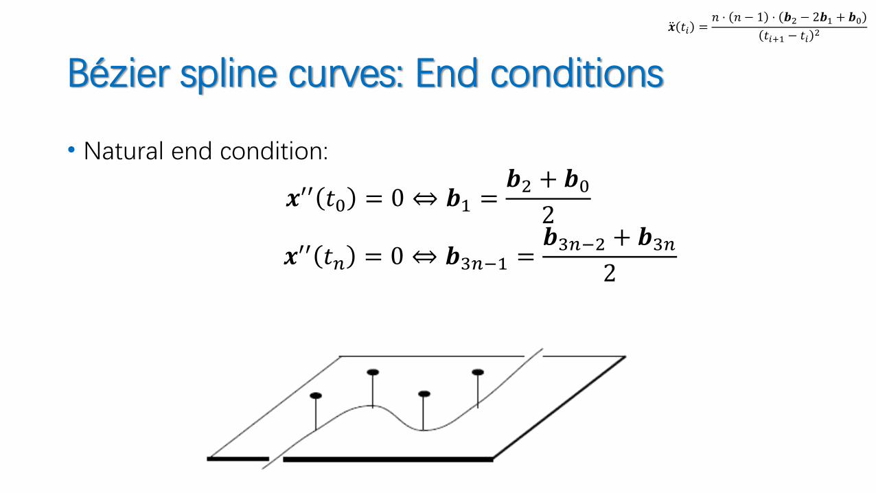
• Natural end condition:
𝒙′′ 𝑡0 = 0 ⇔ 𝒃1 =𝒃2 + 𝒃0
2
𝒙′′ 𝑡𝑛 = 0 ⇔ 𝒃3𝑛−1 =𝒃3𝑛−2 + 𝒃3𝑛
2
ሷ𝒙 𝑡𝑖 =𝑛 ⋅ 𝑛 − 1 ⋅ 𝒃2 − 2𝒃1 + 𝒃0
𝑡𝑖+1 − 𝑡𝑖2
End conditions: Examples
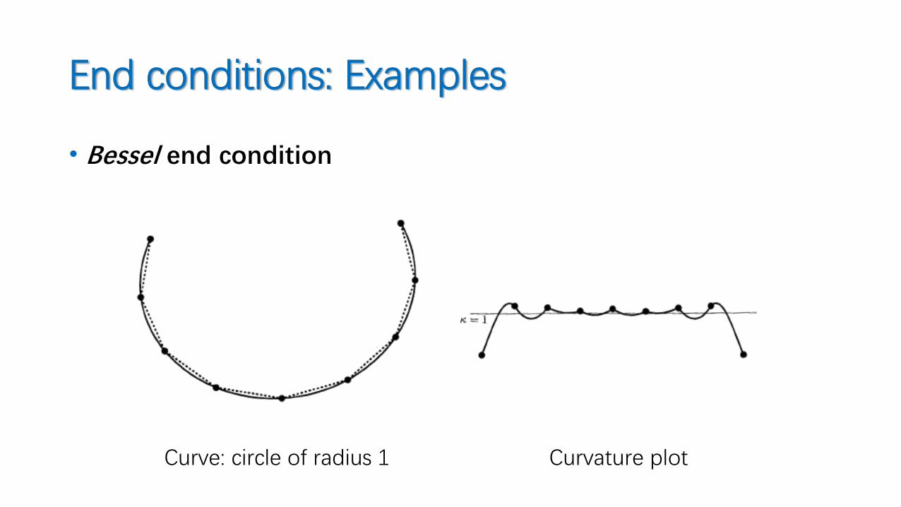
• Bessel end condition
Curve: circle of radius 1 Curvature plot
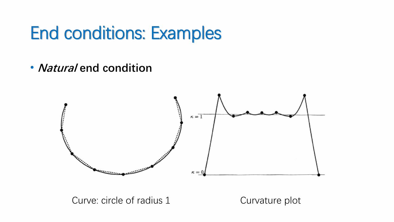
End conditions: Examples
• Natural end condition
Curve: circle of radius 1 Curvature plot

Bézier Splines𝐶2 Cubic Bézier Splines: parameterization
Bézier spline curves: Parameterization
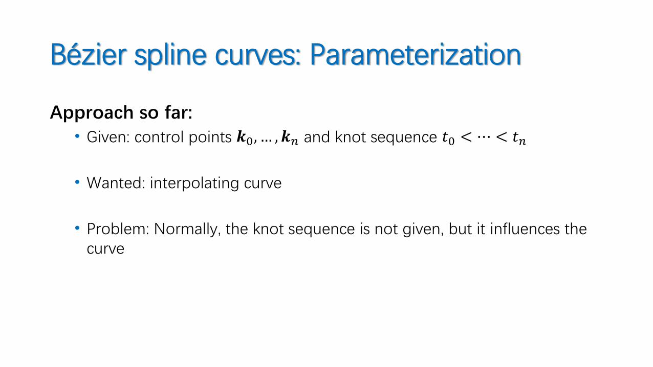
Approach so far:• Given: control points 𝒌0, … , 𝒌𝑛 and knot sequence 𝑡0 < ⋯ < 𝑡𝑛
• Wanted: interpolating curve
• Problem: Normally, the knot sequence is not given, but it influences the curve
Bézier spline curves: Parameterization
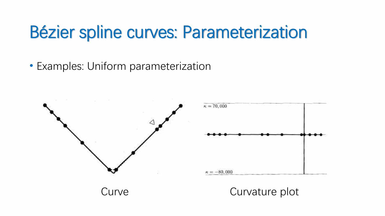
• Equidistant (uniform) parameterization• 𝑡𝑖+1 − 𝑡𝑖 = const
• e.g. 𝑡𝑖 = 𝑖
• Geometry of the data points is not considered
• Chordal parameterization• 𝑡𝑖+1 − 𝑡𝑖 = 𝒌𝑖+1 − 𝒌𝑖• Parameter intervals proportional to the distances of neighbored control
points
Bézier spline curves: Parameterization
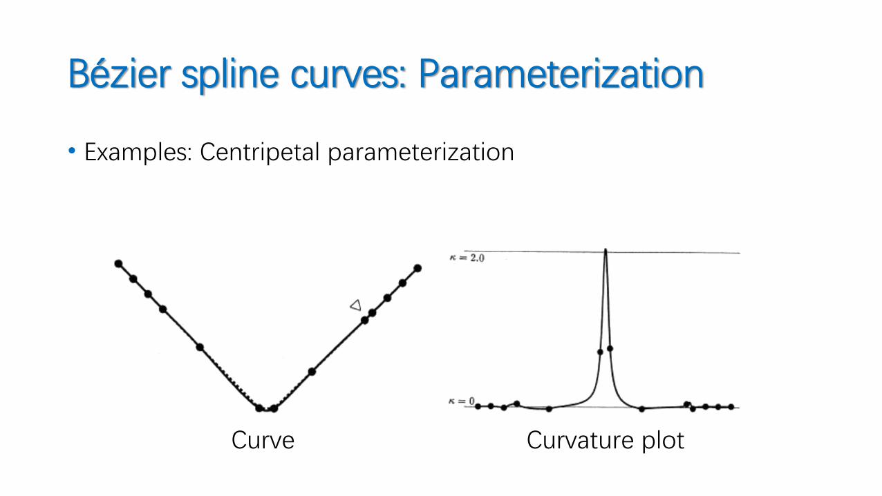
• Centripetal parameterization
• 𝑡𝑖+1 − 𝑡𝑖 = 𝒌𝑖+1 − 𝒌𝑖
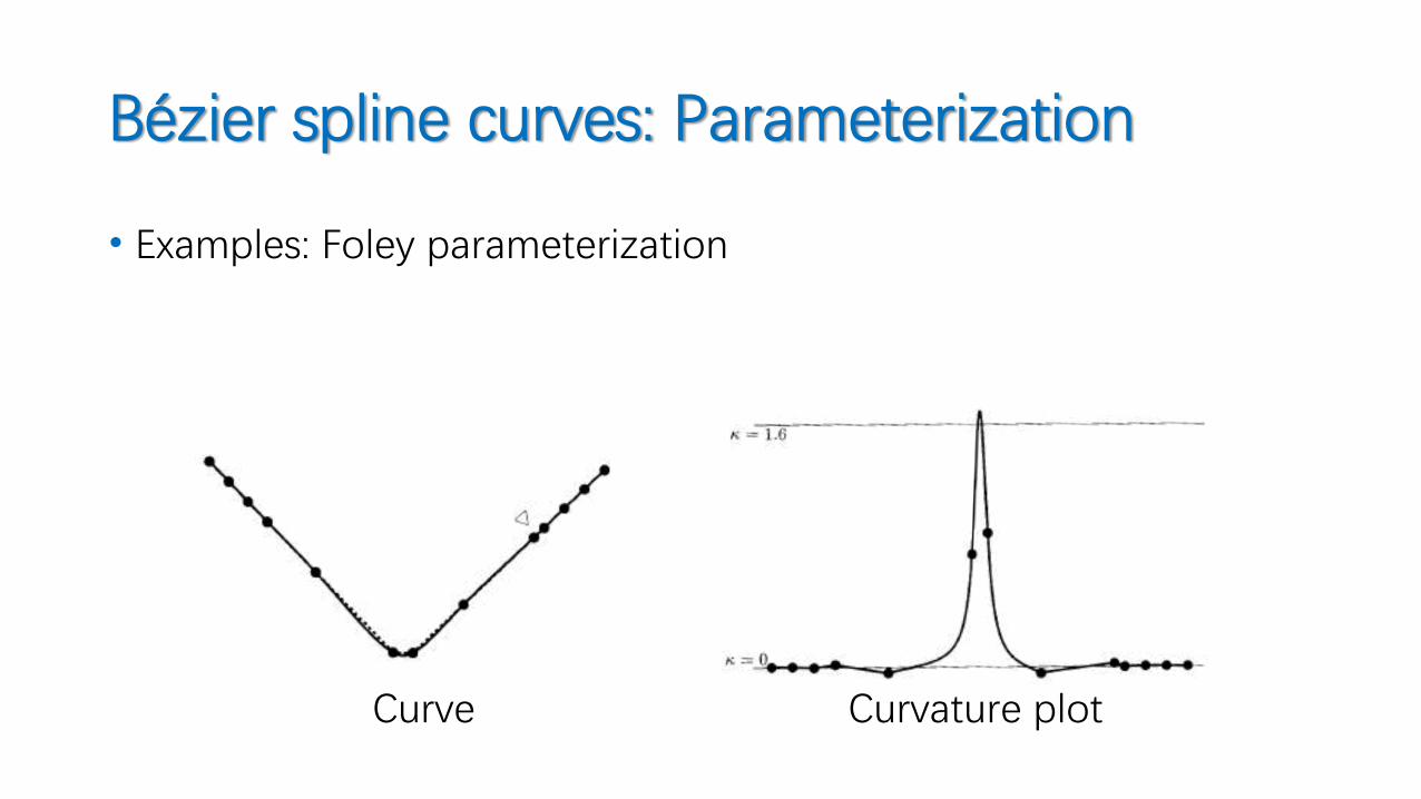
• Foley parameterization• Involvement of angles in the control polygon
• 𝑡𝑖+1 − 𝑡𝑖 = 𝒌𝑖+1 − 𝒌𝑖 ⋅ 1 +3
2
ෝ𝛼𝑖 𝒌𝑖−𝒌𝑖−1
𝒌𝑖−𝒌𝑖−1 + 𝒌𝑖+1−𝒌𝑖+
3
2
ෝ𝛼𝑖+1 𝒌𝑖+1−𝒌𝑖
𝒌𝑖+1−𝒌𝑖 + 𝒌𝑖+2−𝒌𝑖+1
• with ො𝛼𝑖 = min 𝜋 − 𝛼𝑖 ,𝜋
2
• and 𝛼𝑖 = angle 𝒌𝑖−1, 𝒌𝑖 , 𝒌𝑖+1
• Affine invariant parameterization• Parameterization on the basis of an affine invariant distance measure (e.g. G. Nielson)
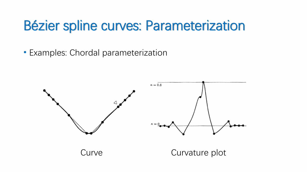
Bézier spline curves: Parameterization
• Examples: Chordal parameterization
Curve Curvature plot
Bézier spline curves: Parameterization
• Examples: Centripetal parameterization
Curve Curvature plot
Bézier spline curves: Parameterization
• Examples: Foley parameterization
Curve Curvature plot
Bézier spline curves: Parameterization
• Examples: Uniform parameterization
Curve Curvature plot

Bézier Splines𝐶2 Cubic Bézier Splines: closed curves
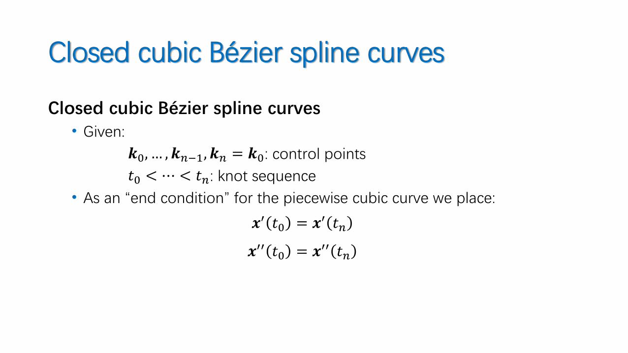
Closed cubic Bézier spline curves
Closed cubic Bézier spline curves• Given:
𝒌0, … , 𝒌𝑛−1, 𝒌𝑛 = 𝒌0: control points
𝑡0 < ⋯ < 𝑡𝑛: knot sequence
• As an “end condition” for the piecewise cubic curve we place:
𝒙′ 𝑡0 = 𝒙′ 𝑡𝑛
𝒙′′ 𝑡0 = 𝒙′′ 𝑡𝑛
Closed cubic Bézier spline curves
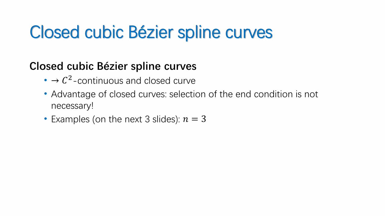
Closed cubic Bézier spline curves• → 𝐶2-continuous and closed curve
• Advantage of closed curves: selection of the end condition is not necessary!
• Examples (on the next 3 slides): 𝑛 = 3
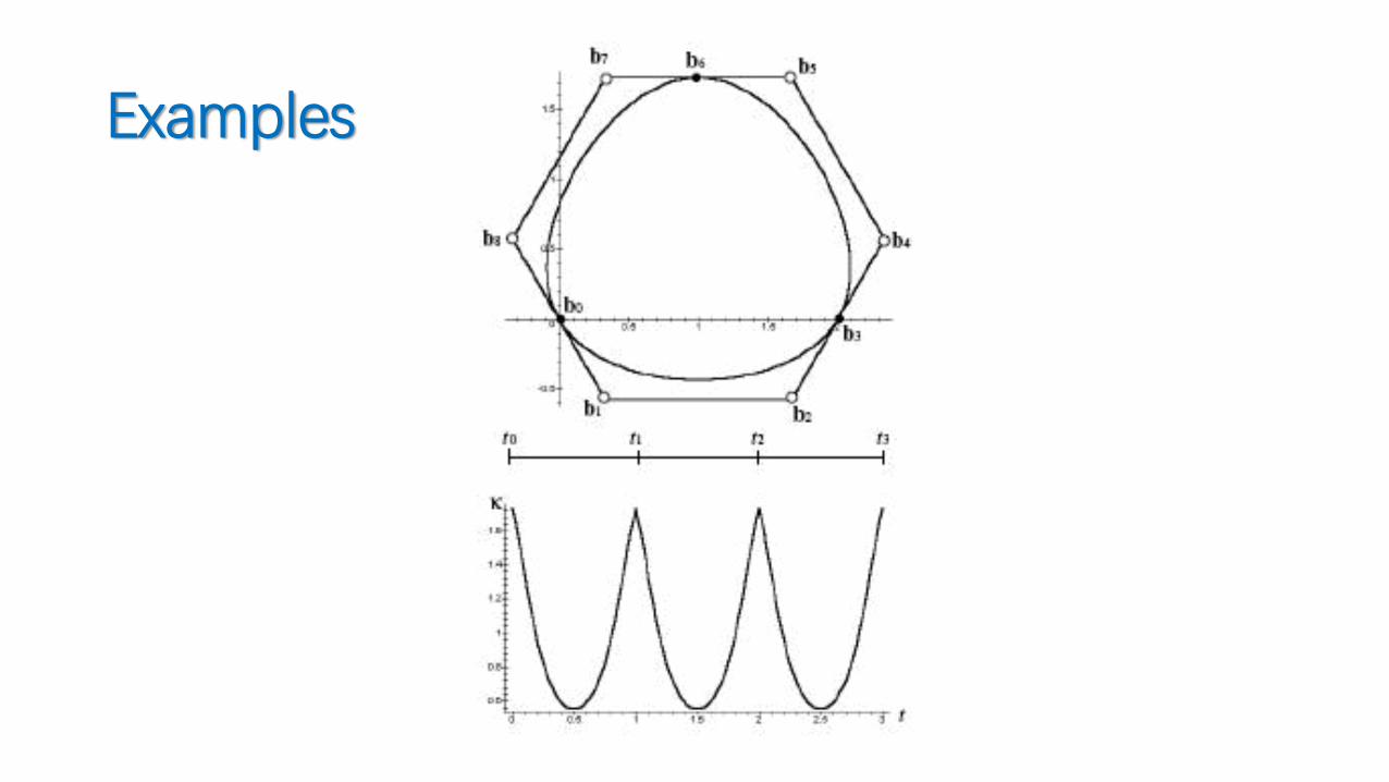
Examples
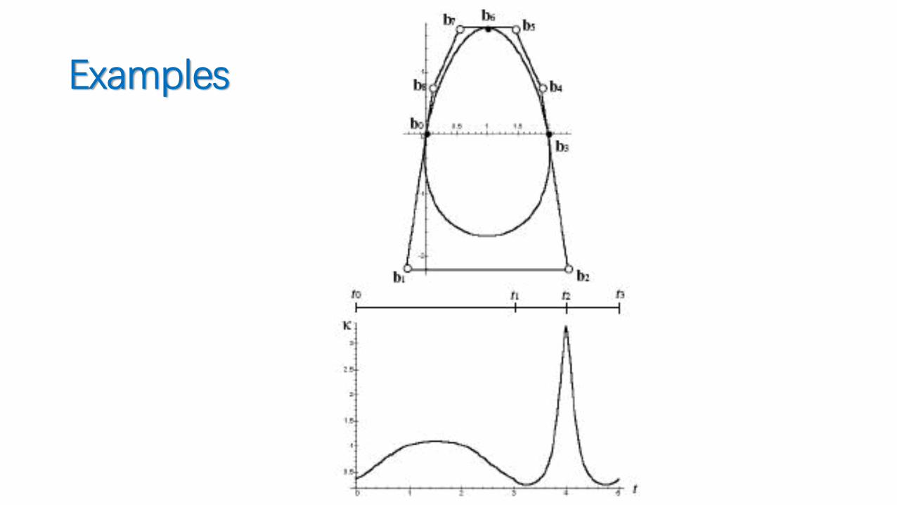
Examples
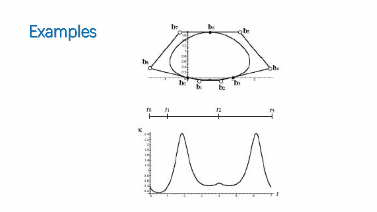
Examples