人类群体遗传学基本原理和分析方法

中科院 - 马普学会计算生物学伙伴研究所

中国科学院上海生命科学研究院研究生课程 人类群体遗传学

徐书华 金 力

第六讲第六讲

人群遗传结构分析人群遗传结构分析 （（ II ））

第四讲第四讲►群体遗传学中的基本概念（群体遗传学中的基本概念（ 44 ））►群体遗传结构群体遗传结构►描述群体遗传结构的统计量描述群体遗传结构的统计量

Hierarchical Hierarchical F F statisticsstatistics►软件演示软件演示

利用利用 ArlequinArlequin 计算人群的计算人群的 Hierarchical Hierarchical F F statstatisticsistics

什么是遗传结构？什么是遗传结构？►从从差异差异中发现中发现结构结构！！►遗传多态性在时间上和空间上的不同分布 遗传多态性在时间上和空间上的不同分布 模式就是模式就是遗传结构遗传结构。。时间：不同时代；时间：不同时代；

不同世代。不同世代。空间：不同地理分布；空间：不同地理分布；

同域不同人群；同域不同人群；不同基因组区域。不同基因组区域。

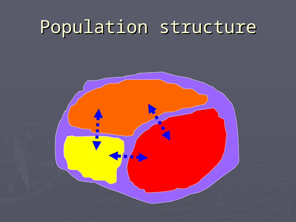
Population structurePopulation structure

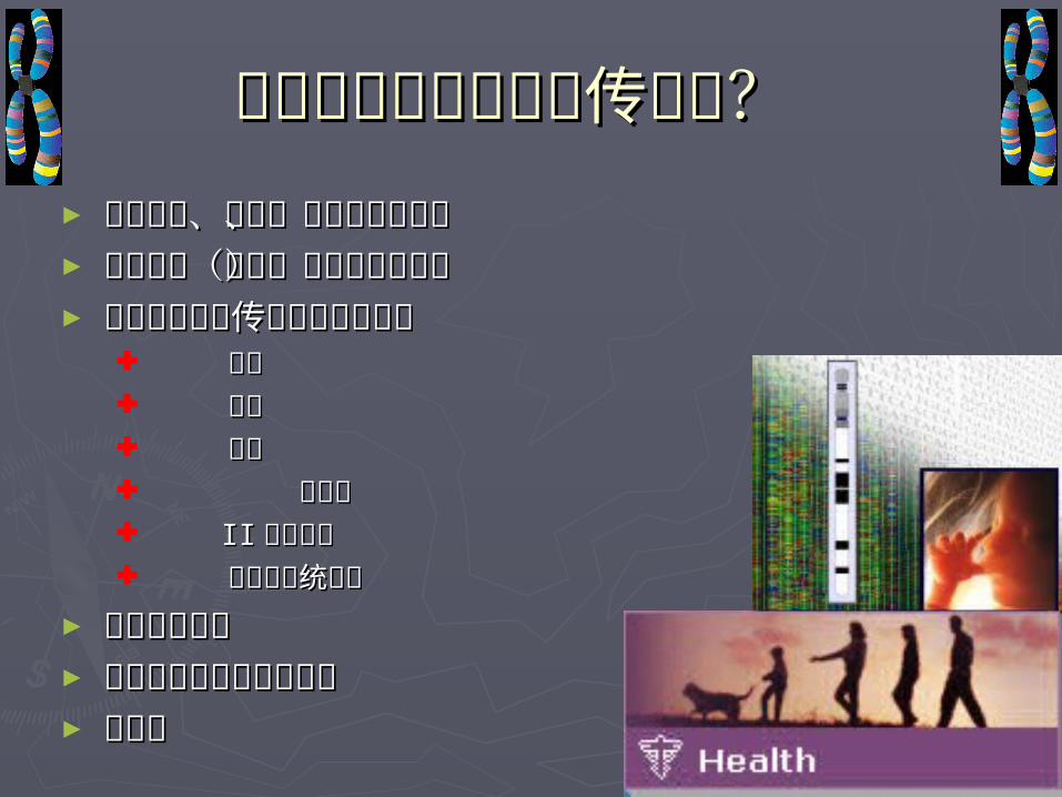
为什么研究人类的遗传结构？为什么研究人类的遗传结构？ ► 人类起源、迁徙、进化历史及前景人类起源、迁徙、进化历史及前景► 现代人群（民族）之间的亲缘关系现代人群（民族）之间的亲缘关系► 复杂疾病的遗传基础和基因定位复杂疾病的遗传基础和基因定位

癌症癌症 肥胖肥胖 哮喘哮喘 精神病精神病 IIII 型糖尿病型糖尿病 心血管系统疾病心血管系统疾病

► 公共卫生保健公共卫生保健► 个性化用药和个性化治疗个性化用药和个性化治疗► 法医学法医学

An exampleAn example

►Population structures and Population structures and association studiesassociation studies

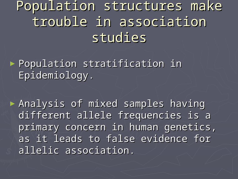
Population structures make Population structures make trouble in association trouble in association

studiesstudies

►Population stratification in Population stratification in Epidemiology.Epidemiology.

►Analysis of mixed samples having Analysis of mixed samples having different allele frequencies is a different allele frequencies is a primary concern in human genetics, primary concern in human genetics, as it leads to false evidence for as it leads to false evidence for allelic association.allelic association.

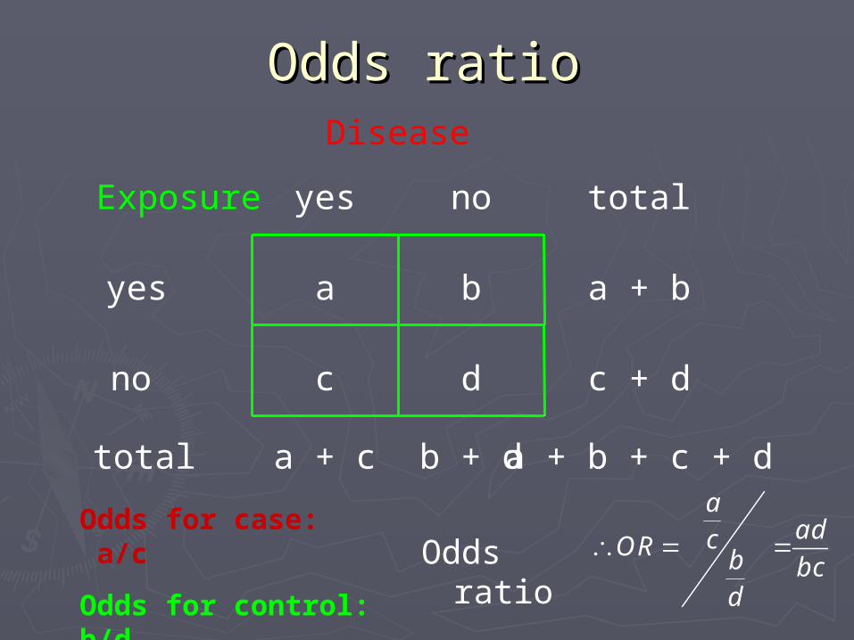
Odds ratioOdds ratio

aadcOR b bc

d

Odds ratioOdds for case: a/c

Odds for control: b/d

Disease

Exposure yes no total

yes a b a + b

no c d c + d

total a + c b + d a + b + c + d

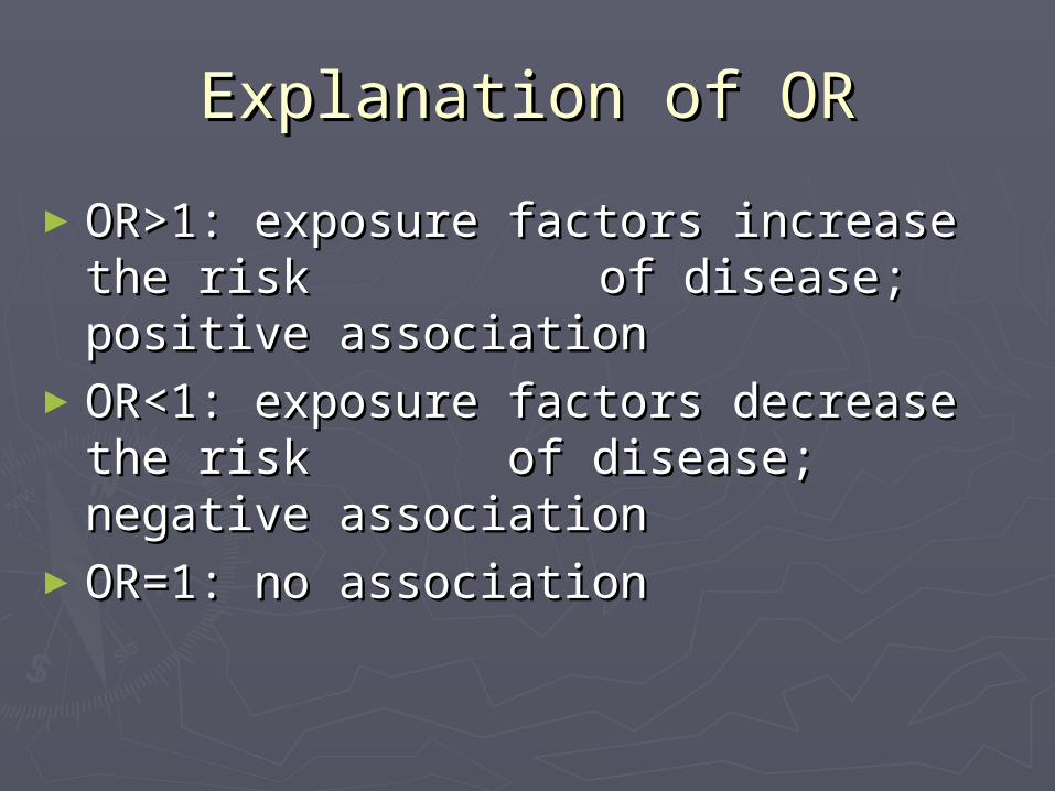
Explanation of ORExplanation of OR

►OR>1: exposure factors increase OR>1: exposure factors increase the risk the risk of disease; of disease; positive associationpositive association

►OR<1: exposure factors decrease OR<1: exposure factors decrease the risk the risk of disease; of disease; negative associationnegative association

►OR=1: no associationOR=1: no association

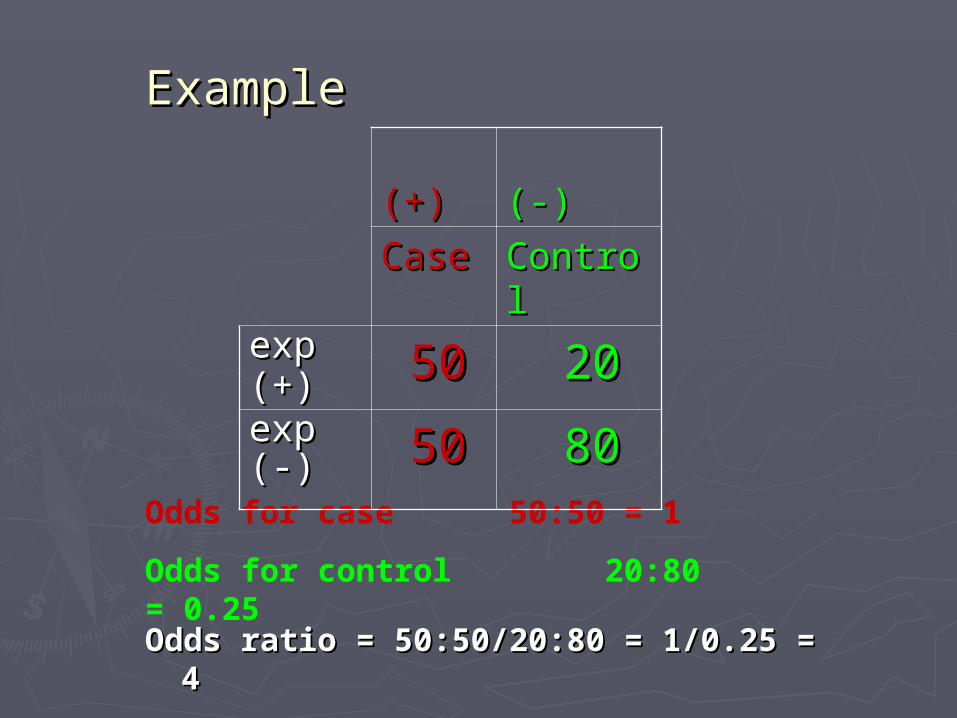
Odds for case 50:50 = 1

Odds for control 20:80 = 0.25

(+)(+)

(-)(-)

CaseCase ControControll

expexp(+)(+) 5050 2020expexp(-)(-) 5050 8080

Example Example

Odds ratio = 50:50/20:80 = 1/0.25 = 4Odds ratio = 50:50/20:80 = 1/0.25 = 4

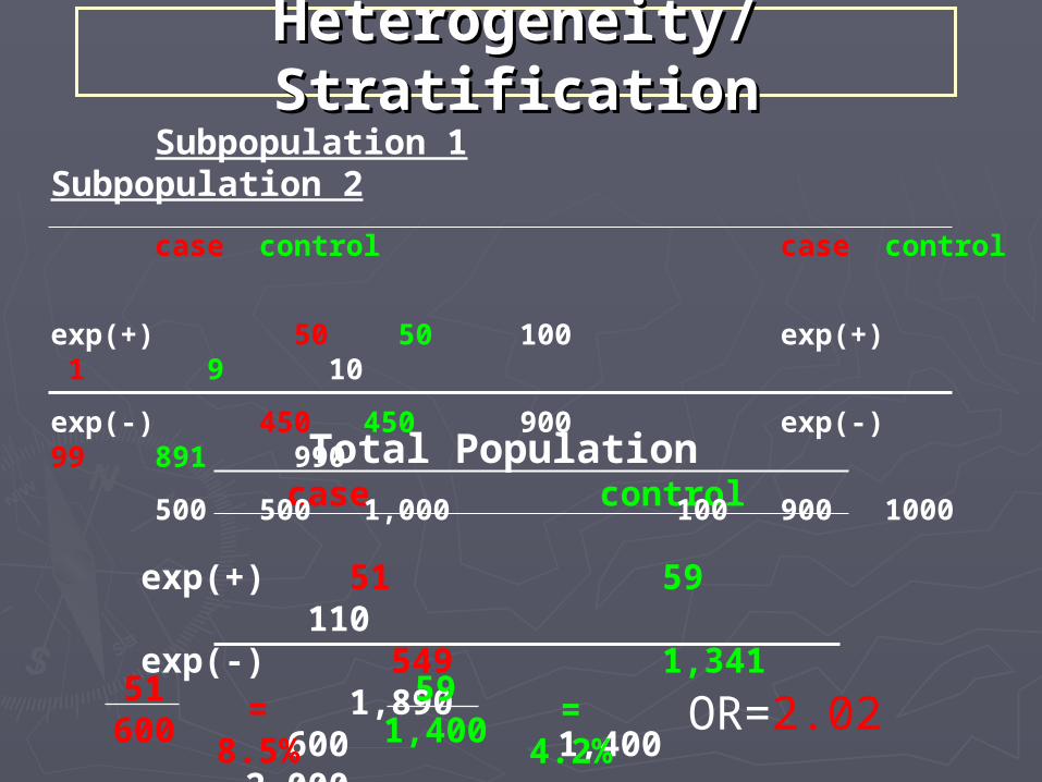
Total Population case control

exp(+) 51 59 110

exp(-) 549 1,3411,890

600 1,4002,000

Heterogeneity/Heterogeneity/StratificationStratification

Subpopulation 1Subpopulation 2

case control case control

exp(+) 50 50 100 exp(+) 1 9 10

exp(-) 450 450 900 exp(-) 99 891 990

500 500 1,000 100 900 1000

= 8.5%

= 4.2%

51600

591,400 OR=2.02

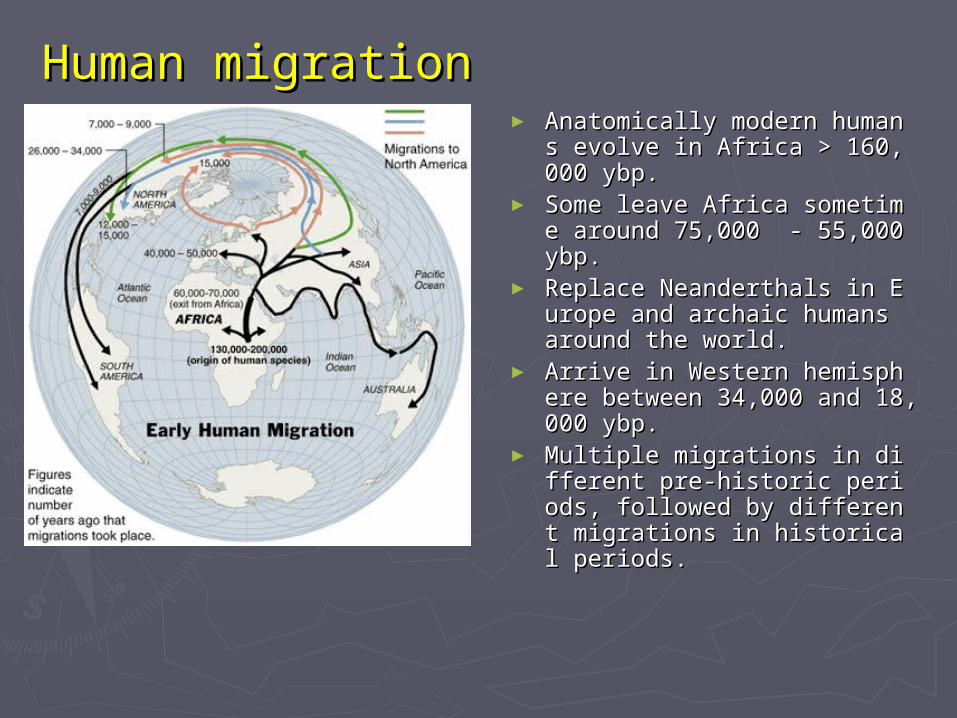
Human migrationHuman migration► Anatomically modern humans Anatomically modern humans

evolve in Africa > 160,000 evolve in Africa > 160,000 ybp.ybp.

► Some leave Africa sometime Some leave Africa sometime around 75,000 - 55,000 ybp.around 75,000 - 55,000 ybp.

► Replace Neanderthals in EurReplace Neanderthals in Europe and archaic humans arouope and archaic humans around the world.nd the world.

► Arrive in Western hemispherArrive in Western hemisphere between 34,000 and 18,000 e between 34,000 and 18,000 ybp.ybp.

► Multiple migrations in diffMultiple migrations in different pre-historic periods, erent pre-historic periods, followed by different migrafollowed by different migrations in historical periods.tions in historical periods.

Note on Definitions: Note on Definitions: Biological RaceBiological Race

►morphology (phenotype)morphology (phenotype)►Geographical locationGeographical location►Population based (frequency of Population based (frequency of genes)genes)

Socially Constructed Race: Arbitrarily utilizes aspects of morphology, geography, culture, language, religion, etc. in the service of asocial dominance hierarchy.

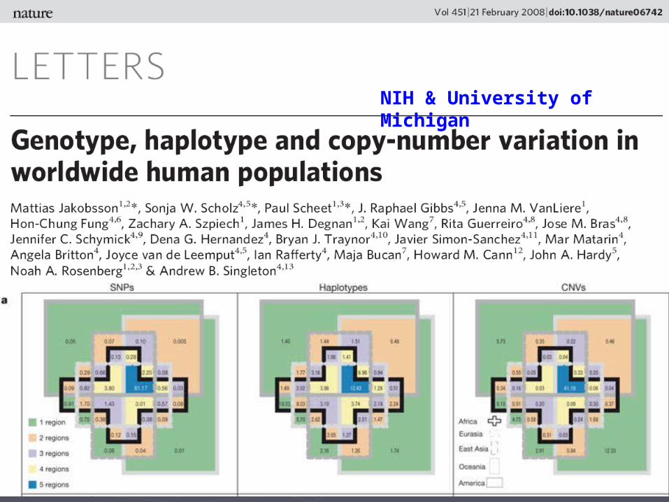
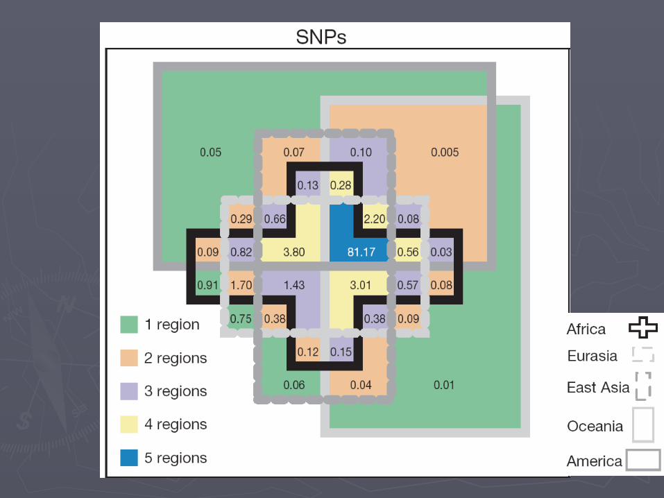
NIH & University of Michigan

描述遗传结构的统计量描述遗传结构的统计量►Hierarchical Hierarchical F F statisticsstatistics

固定指数固定指数► 固定指数（固定指数（ FF ）） ::► 如果一个座位上有两个等位基因，如果一个座位上有两个等位基因， Hardy-WeinbergHardy-Weinberg 比率的比率的

任何偏差可以由参量任何偏差可以由参量 FF 来度量，来度量， FF 称为固定指数，则基因型称为固定指数，则基因型频率可以由下式给出：频率可以由下式给出：

211 1 1

12 1 2

222 2 2

(1 )

2(1 )

(1 )

X F x Fx

X F x x

X F x Fx

► 由以上第二式可得：由以上第二式可得：

1 2 12 1 2(2 ) /(2 )F x x X x x

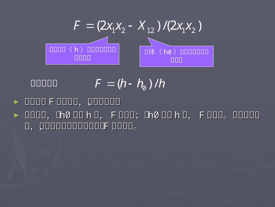
1 2 12 1 2(2 ) /(2 )F x x X x x

► 固定指数固定指数 FF 可正可负，视情况而定。可正可负，视情况而定。► 可以看出，当可以看出，当 h0h0 小于小于 hh 时，时， FF 取正值；当取正值；当 h0h0 大于大于 hh 时，时， FF

取负值。在近亲交配时，杂合子频率的观察值减小，取负值。在近亲交配时，杂合子频率的观察值减小， FF 就就取正值。取正值。

随机交配（ h ）情况下杂合子的预期频率

群体（ h0 ）中下杂合子的观察频率

0( ) /F h h h 上式可写成

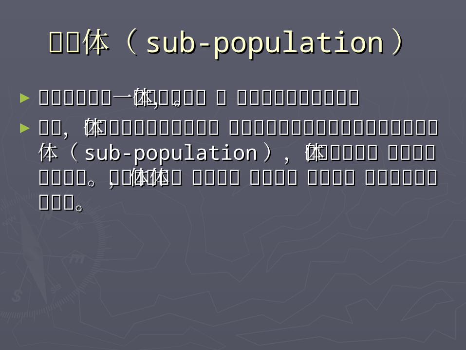
亚群体（亚群体（ sub-populationsub-population ））►以上考虑的是一个简单的群体，不论其是否以上考虑的是一个简单的群体，不论其是否近亲交配。近亲交配。

►然而，实际上大多数的自然群体可被再分为然而，实际上大多数的自然群体可被再分为许多不同的繁殖单位或亚群体（许多不同的繁殖单位或亚群体（ sub-populasub-populationtion ），尽管这些群体并不是完全隔离的。），尽管这些群体并不是完全隔离的。这种情况下，研究群体内和群体间的遗传变这种情况下，研究群体内和群体间的遗传变异就显得十分重要。异就显得十分重要。

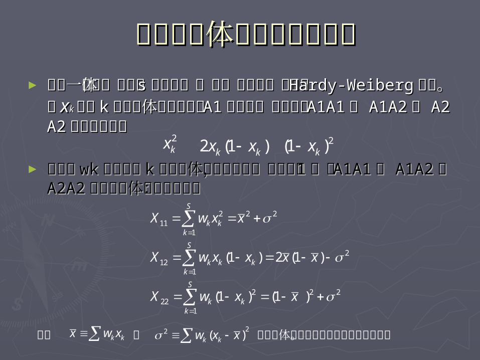
可再分群体中的基因型频率可再分群体中的基因型频率► 假定一个群体可分为假定一个群体可分为 ss 个亚群体，每一个亚群体都满足个亚群体，每一个亚群体都满足 HaHa

rdy-Weibergrdy-Weiberg平衡。设平衡。设 xxkk为第为第 kk个亚群体中等位基因个亚群体中等位基因 A1A1的频率，则基因型的频率，则基因型 A1A1A1A1 ，， A1A2A1A2，， A2A2A2A2的频率分别为的频率分别为

2kx 2 (1 )k kx x 2(1 )kx

2 2 211

1

212

1

2 2 222

1

(1 ) 2 (1 )

(1 ) (1 )

S

k kk

S

k k kk

S

k kk

X w x x

X w x x x x

X w x x

k kx w x 22 ( )k kw x x

► 我们用我们用 wkwk来表示第来表示第 kk个亚群体的相对大小，且总和为个亚群体的相对大小，且总和为 11 。。则则 A1A1A1A1 ，， A1A2A1A2，， A2A2A2A2在整个群体中的频率为：在整个群体中的频率为：

其中 和 是亚群体中等位基因频率的均值和方差。

可再分群体中的固定指数可再分群体中的固定指数

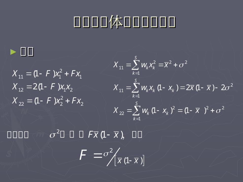
►比较比较2

11 1 1

12 1 2

222 2 2

(1 )

2(1 )

(1 )

X F x Fx

X F x x

X F x Fx

2 2 211

1

211

1

2 2 222

1

(1 ) 2 (1 ) 2

(1 ) (1 )

S

k kk

S

k k kk

S

k kk

X w x x

X w x x x x

X w x x

2 (1 )Fx x 对应于我们知道 ，因此

2

(1 )x xF

►表明如果一个群体被分为多个交配单位，纯合子表明如果一个群体被分为多个交配单位，纯合子的频率要高于的频率要高于 Hardy-WeinbergHardy-Weinberg 比率。这个性质首比率。这个性质首先由先由 WahlundWahlund （（ 19281928 ）发现，被称为）发现，被称为 WahlundWahlund 定定律，也称律，也称 WahlundWahlund 现象。现象。

► 当等位基因频率在所有亚群体中一致时，当等位基因频率在所有亚群体中一致时， FF 为为 00 ；；而当每个亚群体都被固定为某一个等位基因时，而当每个亚群体都被固定为某一个等位基因时，FF 为为 11 。。

WahlundWahlund 定律定律

2

(1 )x xF

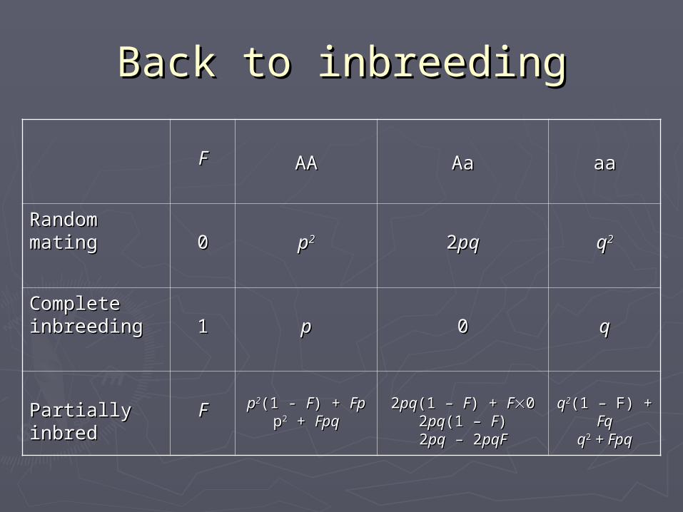
Back to inbreedingBack to inbreeding

FF AAAA AaAa aaaa

RandomRandommatingmating 00 pp22 22pqpq qq22

Complete Complete inbreedinginbreeding 11 pp 00 qq

Partially Partially inbredinbred

FF pp22(1 - (1 - FF) + ) + FpFppp22 + + FpqFpq

22pqpq(1 – (1 – FF) + ) + FF0022pqpq(1 – (1 – FF))22pqpq – 2 – 2pqFpqF

qq22(1 – F) + (1 – F) + FFqq

qq22 + Fpq + Fpq

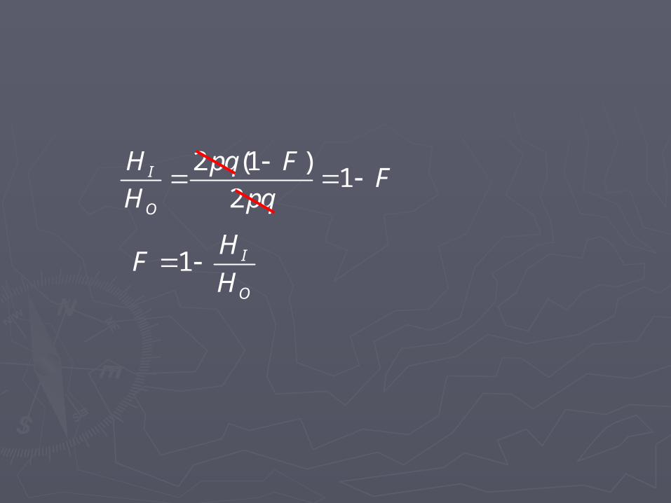
2 (1 )1

2I

O

H pq FF

H pq

1 I

O

HF

H

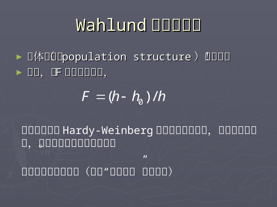
WahlundWahlund 现象的启示现象的启示► 群体结构（群体结构（ population structurepopulation structure ）的存在！）的存在！►反之，当反之，当 FF 为负值的时候，为负值的时候，

0( ) /F h h h

杂合子频率比 Hardy-Weinberg平衡时预期的要高，意味着杂合优势，某种程度的自然选择发生。

杂合优势与平衡选择（后面“自然选择”章节细谈）

Wright’s Fixation Wright’s Fixation Index (Index (FFSTST))

Sewall Wright1889-1988

FF-statistics-statistics

►Different Different FF-statistics for different -statistics for different scalesscales Individual (I)Individual (I) Subpopulation (S)Subpopulation (S) Total population (T)Total population (T)

►Those are the traditional scales but Those are the traditional scales but in theory there can be no limit to the in theory there can be no limit to the # of levels of analysis .# of levels of analysis .

►Originally defined for 2 allelesOriginally defined for 2 alleles►Extended to >2 alleles as Extended to >2 alleles as G-G-statisticsstatistics

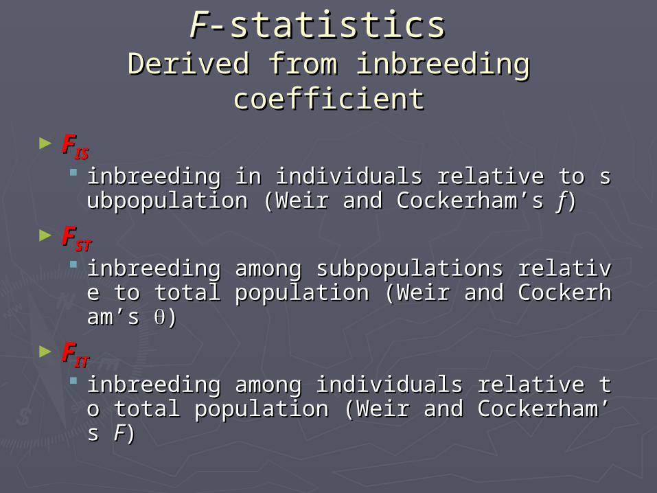
FF-statistics -statistics Derived from inbreeding Derived from inbreeding

coefficientcoefficient►FFISIS

inbreeding in individuals relative to subpoinbreeding in individuals relative to subpopulation (Weir and Cockerham’s pulation (Weir and Cockerham’s ff))

►FFSTST inbreeding among subpopulations relative to inbreeding among subpopulations relative to total population (Weir and Cockerham’s total population (Weir and Cockerham’s ))

►FFITIT inbreeding among individuals relative to toinbreeding among individuals relative to total population (Weir and Cockerham’s tal population (Weir and Cockerham’s FF))

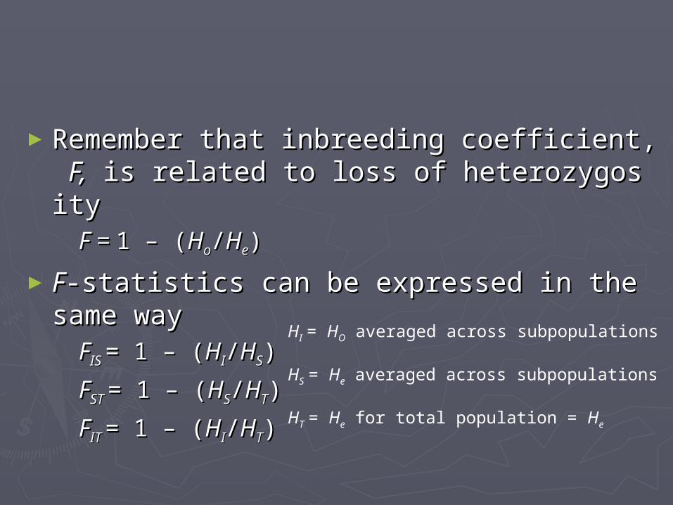
►Remember that inbreeding coefficient, Remember that inbreeding coefficient, F,F, is related to loss of heterozygosity is related to loss of heterozygosity

F = F = 1 – (1 – (HHoo//HHee))►FF-statistics can be expressed in the sa-statistics can be expressed in the same wayme way

FFIS IS = 1 – (= 1 – (HHII//HHSS))FFST ST = 1 – (= 1 – (HHSS//HHTT))FFIT IT = 1 – (= 1 – (HHII//HHTT))

HI = HO averaged across subpopulations

HS = He averaged across subpopulations

HT = He for total population = He

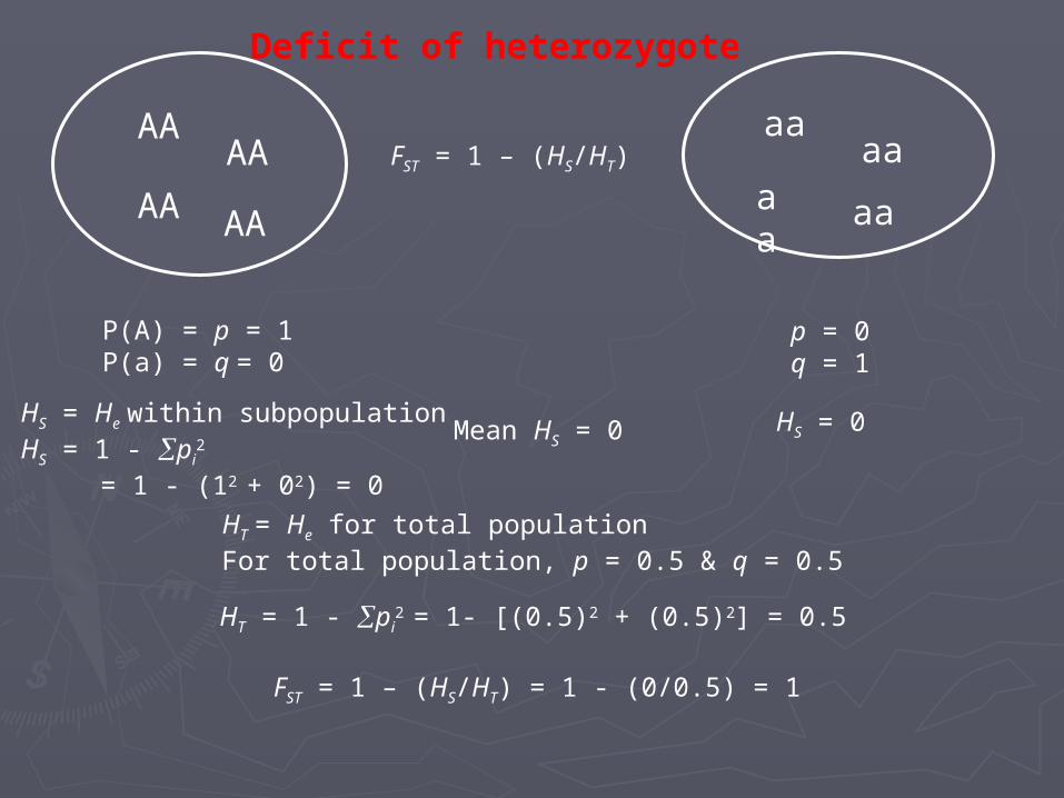
AA AA

AAAA

aa

aaaa

aa

P(A) = p = 1P(a) = q = 0

p = 0q = 1

HS = He within subpopulationHS = 1 - pi

2 = 1 - (12 + 02) = 0

HS = 0Mean HS = 0

HT = 1 - pi2 = 1- [(0.5)2 + (0.5)2] = 0.5

FST = 1 – (HS/HT) = 1 - (0/0.5) = 1

HT = He for total populationFor total population, p = 0.5 & q = 0.5

FST = 1 – (HS/HT)

Deficit of heterozygote

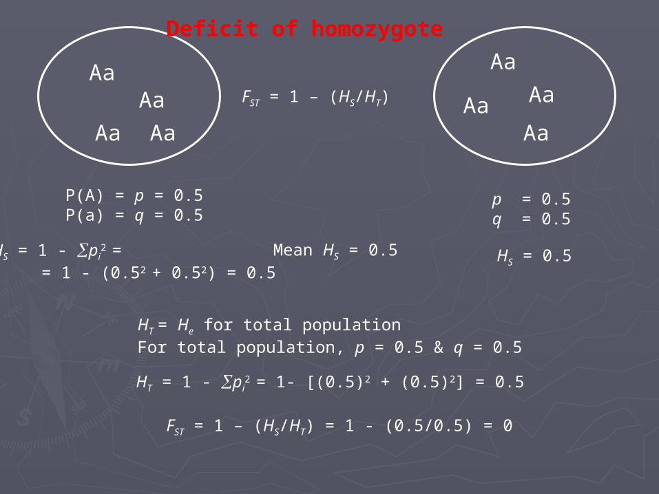
Aa

Aa Aa

Aa AaAa

Aa

Aa

P(A) = p = 0.5P(a) = q = 0.5

p = 0.5q = 0.5

HS = 1 - pi2 =

= 1 - (0.52 + 0.52) = 0.5HS = 0.5Mean HS = 0.5

FST = 1 – (HS/HT)

HT = 1 - pi2 = 1- [(0.5)2 + (0.5)2] = 0.5

FST = 1 – (HS/HT) = 1 - (0.5/0.5) = 0

HT = He for total populationFor total population, p = 0.5 & q = 0.5

Deficit of homozygote

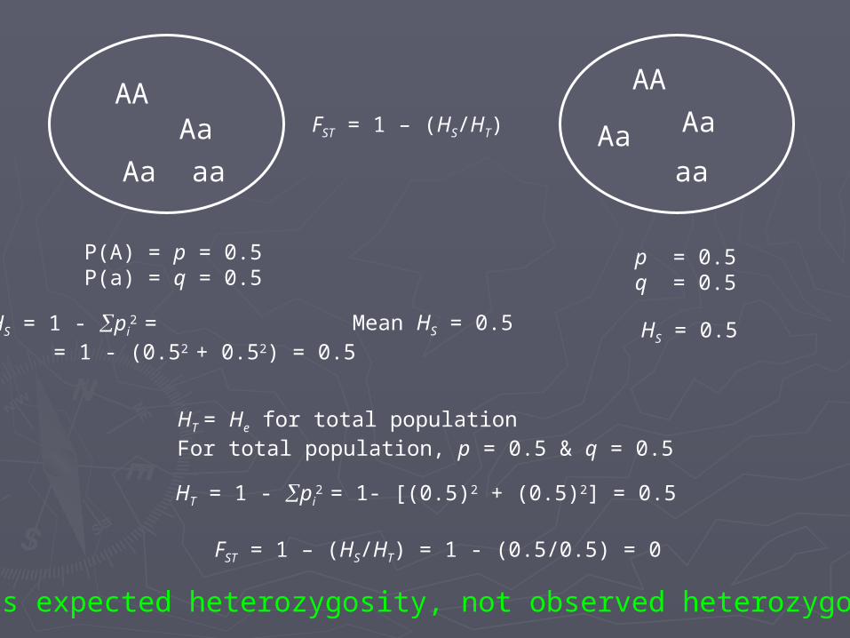
AA

Aa aa

Aa Aaaa

AA

AaFST = 1 – (HS/HT)

P(A) = p = 0.5P(a) = q = 0.5

p = 0.5q = 0.5

HS = 1 - pi2 =

= 1 - (0.52 + 0.52) = 0.5HS = 0.5Mean HS = 0.5

HT = 1 - pi2 = 1- [(0.5)2 + (0.5)2] = 0.5

FST = 1 – (HS/HT) = 1 - (0.5/0.5) = 0

HT = He for total populationFor total population, p = 0.5 & q = 0.5

FST uses expected heterozygosity, not observed heterozygosity!!

F statisticsF statistics► FFISIS tells us if there is inbreeding within subpo tells us if there is inbreeding within subpo

pulations by comparing Hpulations by comparing HII and H and HSS::

► Bars mean that the values are the averages over Bars mean that the values are the averages over all the subpopulations that we are considering. all the subpopulations that we are considering.

► So FSo FISIS measures whether there is, on average, a measures whether there is, on average, a deficit of heterozygotes within subpopulations.deficit of heterozygotes within subpopulations.

S IIS

S

H HF

H

F statisticsF statistics

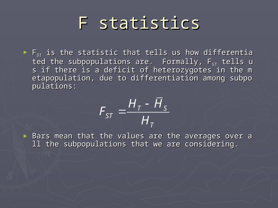
► FFSTST is the statistic that tells us how differentiated is the statistic that tells us how differentiated the subpopulations are. Formally, Fthe subpopulations are. Formally, FSTST tells us if th tells us if there is a deficit of heterozygotes in the metapopulatere is a deficit of heterozygotes in the metapopulation, due to differentiation among subpopulations:ion, due to differentiation among subpopulations:

► Bars mean that the values are the averages over all Bars mean that the values are the averages over all the subpopulations that we are considering.the subpopulations that we are considering.

T SST

T

H HF

H

F statisticsF statistics

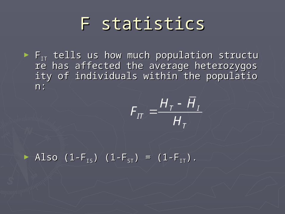
► FFITIT tells us how much population structure has affected the tells us how much population structure has affected the average heterozygosity of individuals within the populatioaverage heterozygosity of individuals within the population:n:

► Also (1-FAlso (1-FISIS) (1-F) (1-FSTST) = (1-F) = (1-FITIT).).

T IIT

T

H HF

H

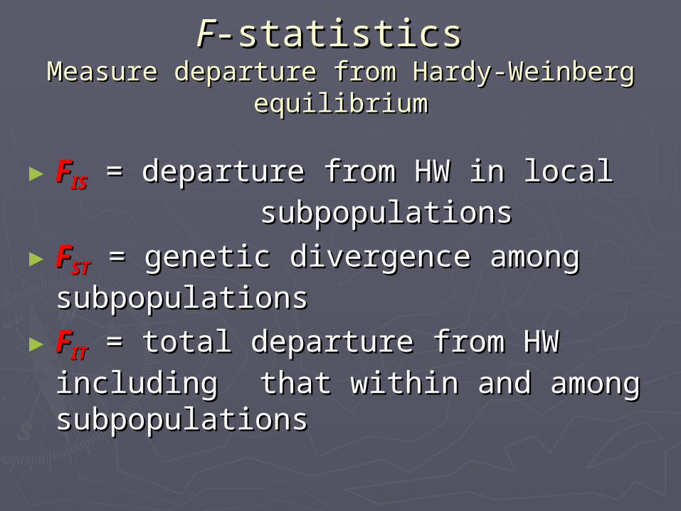
FF-statistics -statistics Measure departure from Hardy-Weinberg Measure departure from Hardy-Weinberg

equilibriumequilibrium

►FFISIS = departure from HW in local = departure from HW in local subpopulationssubpopulations

►FFSTST = genetic divergence among = genetic divergence among subpopulationssubpopulations

►FFITIT = total departure from HW = total departure from HW including including that within and among that within and among subpopulationssubpopulations

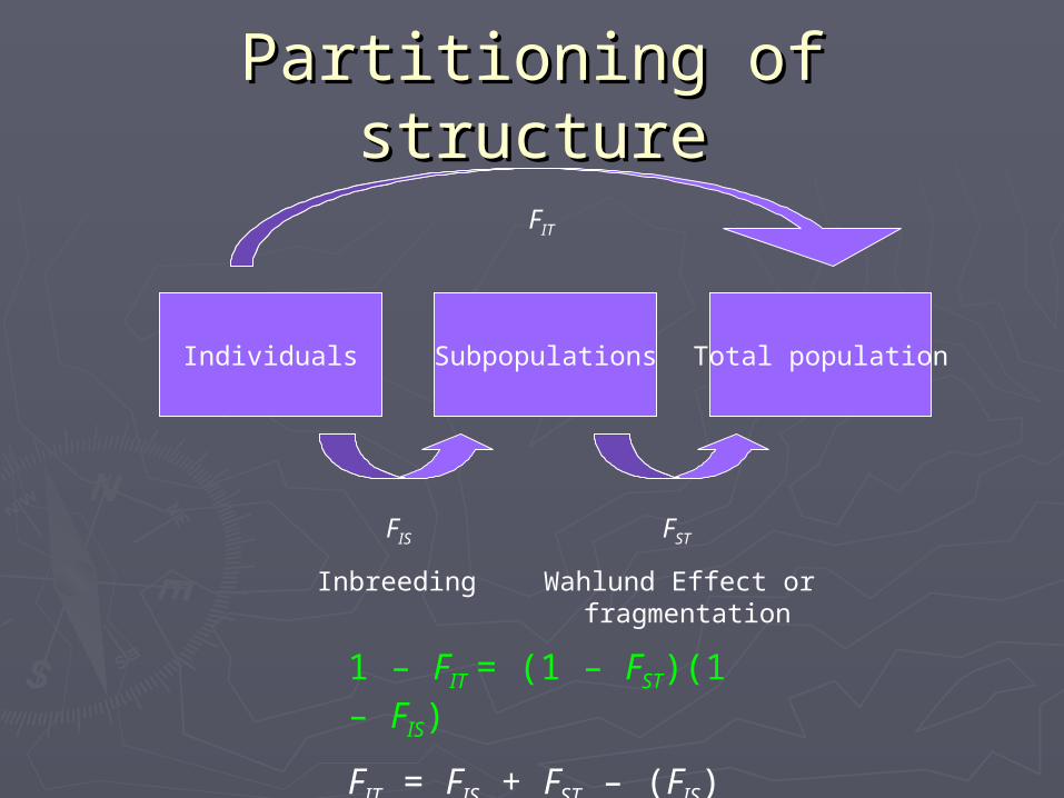
Partitioning of Partitioning of structurestructure

Individuals Subpopulations Total population

FIS FST

FIT

Inbreeding Wahlund Effect or fragmentation

1 – FIT = (1 – FST)(1 – FIS)

FIT = FIS + FST – (FIS)(FST)

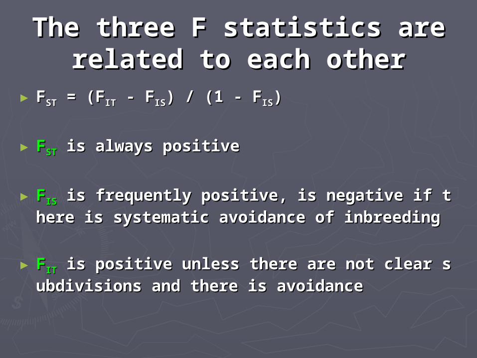
The three F statistics are The three F statistics are related to each otherrelated to each other

► FFSTST = (F = (FITIT - F - FISIS) / (1 - F) / (1 - FISIS))

► FFSTST is always positive is always positive

► FFISIS is frequently positive, is negative if ther is frequently positive, is negative if there is systematic avoidance of inbreedinge is systematic avoidance of inbreeding

► FFITIT is positive unless there are not clear subd is positive unless there are not clear subdivisions and there is avoidanceivisions and there is avoidance

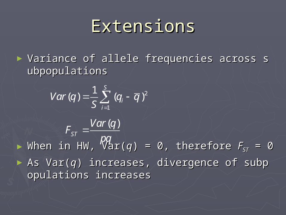
ExtensionsExtensions

► Variance of allele frequencies across subpopVariance of allele frequencies across subpopulationsulations

► When in HW, Var(When in HW, Var(qq) = 0, therefore ) = 0, therefore FFSTST = 0 = 0► As Var(As Var(qq) increases, divergence of subpopula) increases, divergence of subpopula

tions increasestions increases

2

1

1( ) ( )

S

ii

Var q q qS

( )ST

Var qF

pq

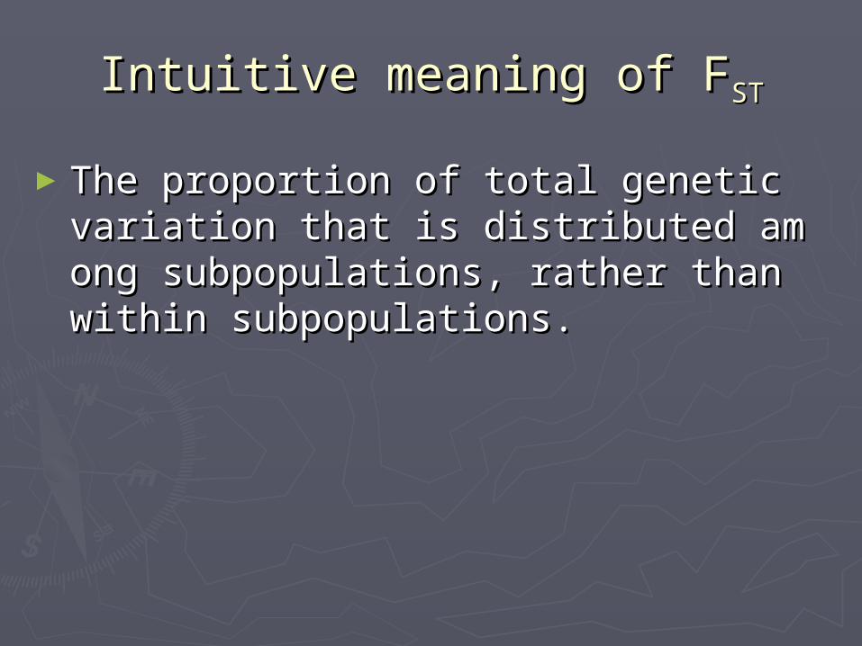
Intuitive meaning of FIntuitive meaning of FSTST

►The proportion of total genetic variatiThe proportion of total genetic variation that is distributed among subpopulaton that is distributed among subpopulations, rather than within subpopulations.ions, rather than within subpopulations.

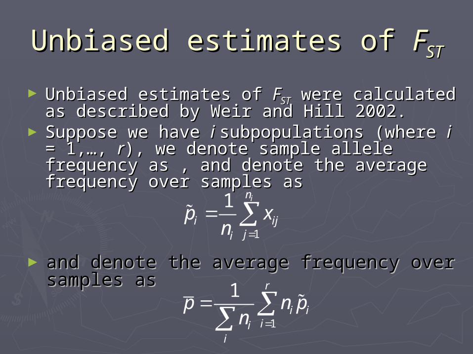
Unbiased estimates of Unbiased estimates of FFSTST

► Unbiased estimates of Unbiased estimates of FFSTST were calculated were calculated as described by Weir and Hill 2002. as described by Weir and Hill 2002.

► Suppose we have Suppose we have i i subpopulations (where subpopulations (where i i = 1,…, = 1,…, rr), we denote sample allele ), we denote sample allele frequency as , and denote the average frequency as , and denote the average frequency over samples as frequency over samples as

1

1 in

i ijji

p xn

1

1 r

i iii

i

p n pn

► and denote the average frequency over and denote the average frequency over samples as samples as

►The observed mean square for loci The observed mean square for loci within populations are denoted by MSG:within populations are denoted by MSG:

1

11

1

r

i i iri

ii

MSG n p pn

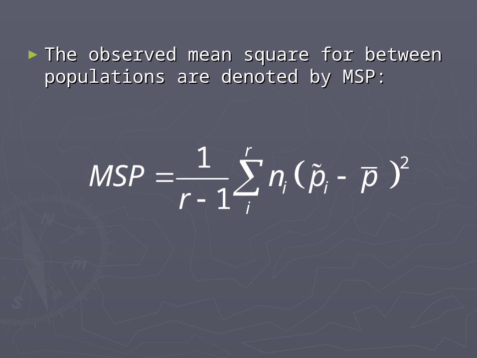
►The observed mean square for between The observed mean square for between populations are denoted by MSP: populations are denoted by MSP:

21

1

r

i ii

MSP n p pr

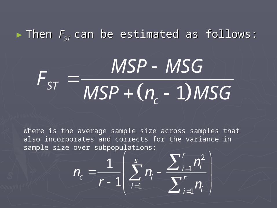
►Then Then FFSTST can be estimated as follows:can be estimated as follows:

1STc

MSP MSGF

MSP n MSG

Where is the average sample size across samples that also incorporates and corrects for the variance in sample size over subpopulations:

2

1

11

1

1

rs

iic i r

i ii

nn n

r n

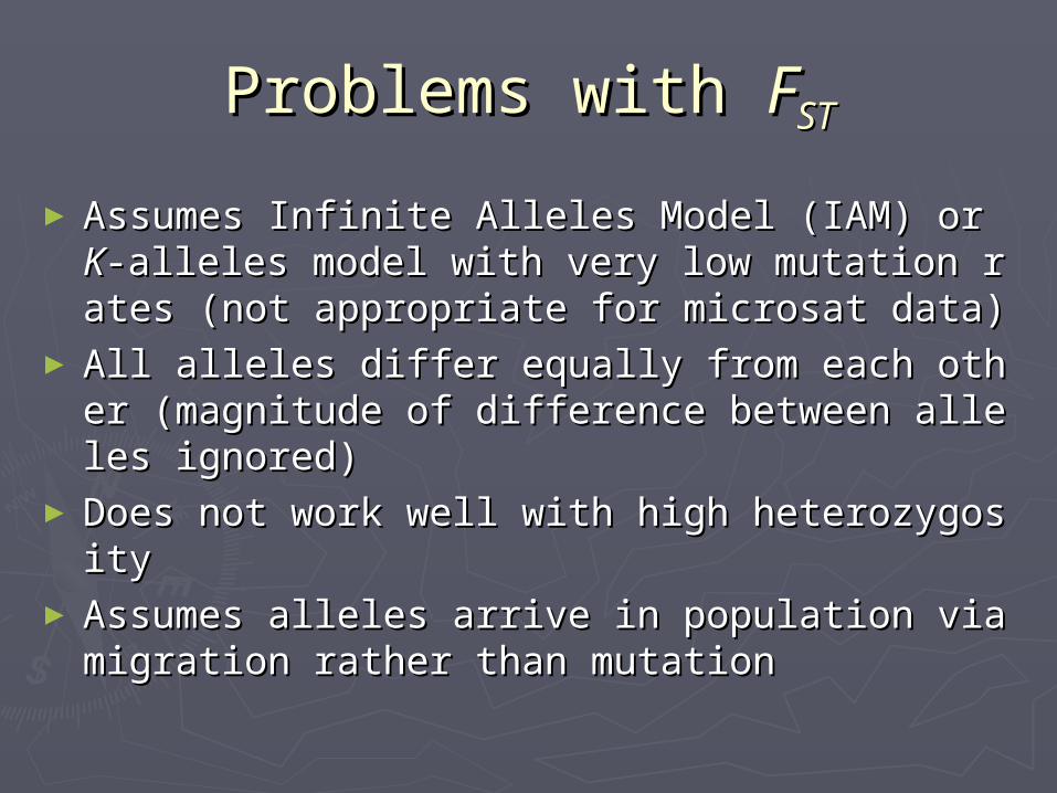
Problems with Problems with FFSTST

► Assumes Infinite Alleles Model (IAM) or Assumes Infinite Alleles Model (IAM) or KK-alleles model with very low mutation rates -alleles model with very low mutation rates (not appropriate for microsat data)(not appropriate for microsat data)

► All alleles differ equally from each other All alleles differ equally from each other (magnitude of difference between alleles ign(magnitude of difference between alleles ignored)ored)

► Does not work well with high heterozygosityDoes not work well with high heterozygosity► Assumes alleles arrive in population via migAssumes alleles arrive in population via mig

ration rather than mutationration rather than mutation

Special version for microsatelliSpecial version for microsatellitestes

► RRSTST (Slatkin 1995) (Slatkin 1995)► Analogue of Analogue of FFSTST

► Assumes Stepwise Mutation Model (mutation model most appropAssumes Stepwise Mutation Model (mutation model most appropriate for microsats)riate for microsats)

► Allows for high mutation ratesAllows for high mutation rates► Allows differences in magnitude between alleles to be accouAllows differences in magnitude between alleles to be accou

nted fornted for

► Where Where SS = average sum of differences in allele sizes in tot = average sum of differences in allele sizes in total population, and al population, and SSWW = average sum within populations = average sum within populations

WST

W

S SR

S

Which to use for Which to use for sats?sats?► FFSTST and and RRSTST can differ using same data can differ using same data► If loci don’t conform to SMM model, If loci don’t conform to SMM model, RRST ST will be underestimatedwill be underestimated

► If mutation rates are large relative to If mutation rates are large relative to migration rates, migration rates, RRSTST is superior is superior

► Longer divergence times between Longer divergence times between populations favors populations favors RRSTST

► RRSTST favored under ideal conditions and favored under ideal conditions and with large sampleswith large samples

► FFSTST favored with small samples and when favored with small samples and when a more conservative estimator is a more conservative estimator is desireddesired

Distance measures for microsatelDistance measures for microsatelliteslites

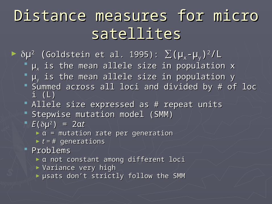
► µµ22 ( (Goldstein et al. 1995):Goldstein et al. 1995): ∑(µ ∑(µxx-µ-µyy))22/L/L µµxx is the mean allele size in population x is the mean allele size in population x µµyy is the mean allele size in population y is the mean allele size in population y Summed across all loci and divided by # of loci (L)Summed across all loci and divided by # of loci (L) Allele size expressed as # repeat unitsAllele size expressed as # repeat units Stepwise mutation model (SMM)Stepwise mutation model (SMM) EE((µµ22) = 2) = 2ααtt

►αα = mutation rate per generation = mutation rate per generation► t = t = # generations# generations

ProblemsProblems►αα not constant among different loci not constant among different loci► Variance very highVariance very high►µsats don’t strictly follow the SMMµsats don’t strictly follow the SMM

Distance measures for microsatelDistance measures for microsatelliteslites

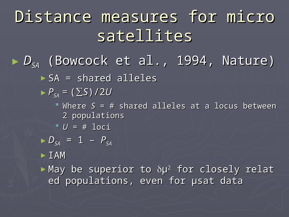
►DDSASA (Bowcock et al., 1994, Nature) (Bowcock et al., 1994, Nature)►SA = shared allelesSA = shared alleles►PPSASA = = (∑(∑SS)/2)/2UU

Where Where SS = # shared alleles at a locus between 2 popu = # shared alleles at a locus between 2 populationslations

UU = # loci = # loci►DDSASA = 1 – = 1 – PPSASA►IAMIAM►May be superior to May be superior to µµ22 for closely related popu for closely related populations, even for µsat datalations, even for µsat data

Degree of Degree of F F statisticsstatistics

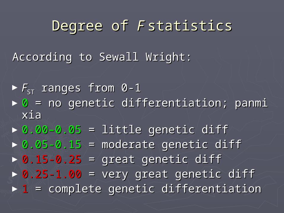
According to Sewall Wright:According to Sewall Wright:

►FFSTST ranges from 0-1 ranges from 0-1►00 = no genetic differentiation; panmixia = no genetic differentiation; panmixia►0.00–0.050.00–0.05 = little genetic diff = little genetic diff►0.05-0.150.05-0.15 = moderate genetic diff = moderate genetic diff►0.15-0.250.15-0.25 = great genetic diff = great genetic diff►0.25-1.000.25-1.00 = very great genetic diff = very great genetic diff►11 = complete genetic differentiation = complete genetic differentiation

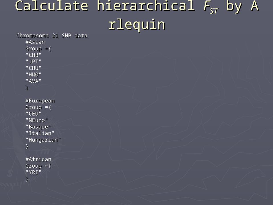
Calculate hierarchical Calculate hierarchical FFSTST by Arlequi by Arlequinn

Chromosome 21 SNP dataChromosome 21 SNP data#Asian#AsianGroup ={Group ={"CHB""CHB""JPT""JPT""CHU""CHU""HMO""HMO""AVA""AVA"}}

#European#EuropeanGroup ={Group ={"CEU""CEU""NEuro""NEuro""Basque""Basque""Italian""Italian""Hungarian""Hungarian"}}

#African#AfricanGroup ={Group ={"YRI""YRI"}}

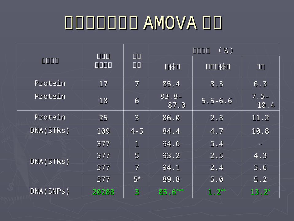
三个大洲人群的三个大洲人群的 AMOVAAMOVA 分析 分析

多态类型多态类型 座位或座位或位点数目位点数目

分组分组数目数目

方差成分 （ 方差成分 （ %% ））

群体内群体内 组内群体间组内群体间 组间组间

ProteinProtein 1717 77 85.485.4 8.38.3 6.36.3

ProteinProtein1818 66

83.8-83.8-87.087.0 5.5-6.65.5-6.6 7.5-7.5-

10.410.4

ProteinProtein 2525 33 86.086.0 2.82.8 11.211.2

DNA(STRs)DNA(STRs) 109109 4-54-5 84.484.4 4.74.7 10.810.8

DNA(STRs)DNA(STRs)

377377 11 94.694.6 5.45.4 --

377377 55 93.293.2 2.52.5 4.34.3

377377 77 94.194.1 2.42.4 3.63.6

377377 55## 89.889.8 5.05.0 5.25.2

DNA(SNPs)DNA(SNPs) 2028820288 33 85.685.6****** 1.21.2**** 13.213.2**

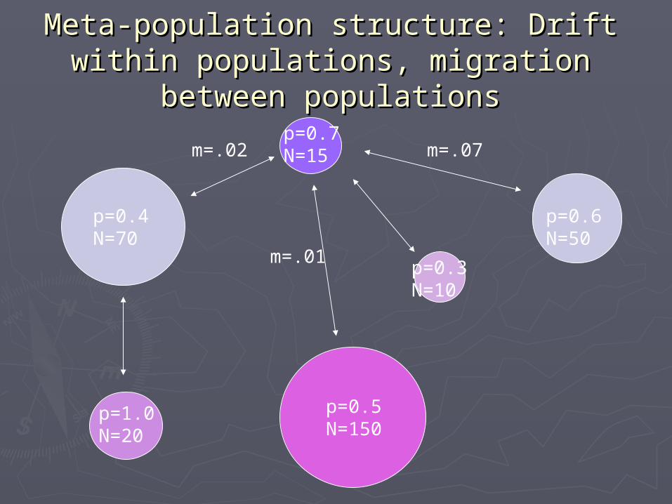
Meta-population structure: Drift Meta-population structure: Drift within populations, migration within populations, migration

between populationsbetween populations

p=0.4N=70

p=0.7N=15

p=1.0N=20

p=0.5N=150

p=0.3N=10

p=0.6N=50

m=.01

m=.07m=.02

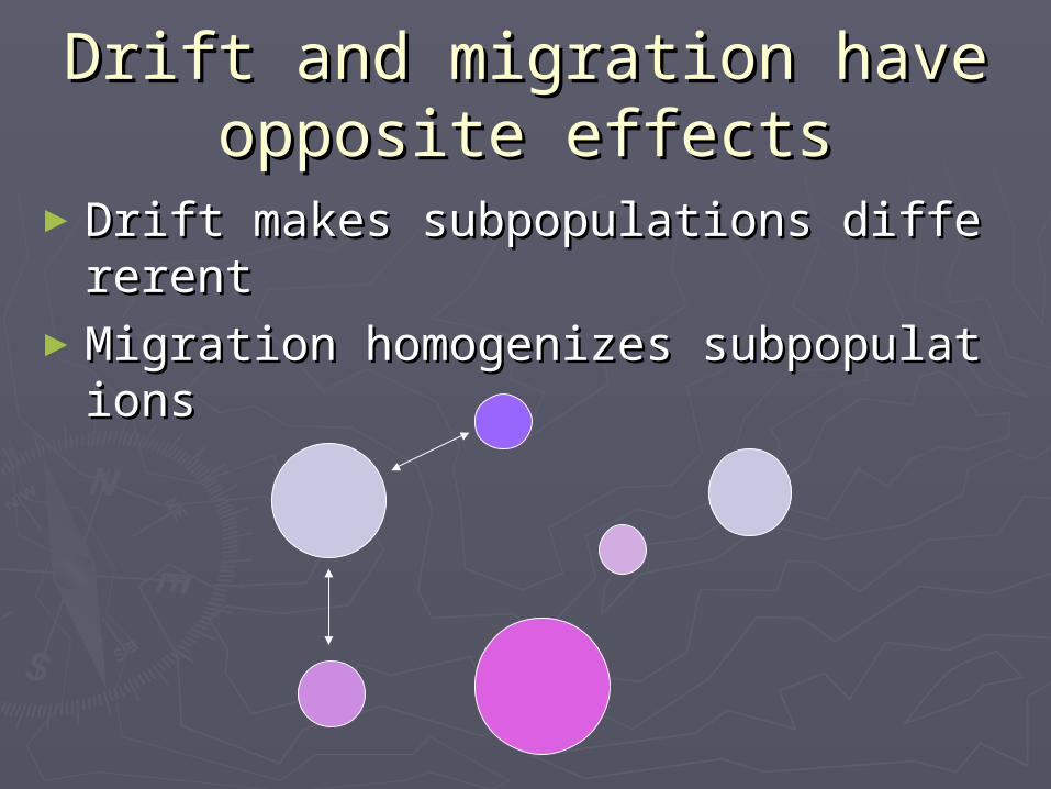
Drift and migration have Drift and migration have opposite effectsopposite effects

►Drift makes subpopulations differerentDrift makes subpopulations differerent►Migration homogenizes subpopulationsMigration homogenizes subpopulations

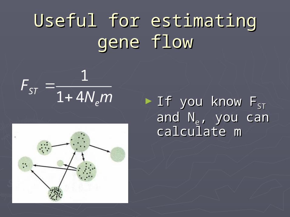
Useful for estimating Useful for estimating gene flowgene flow

►If you know FIf you know FSTST and and NNee, you can calcul, you can calculate mate m

1

1 4STe

FN m

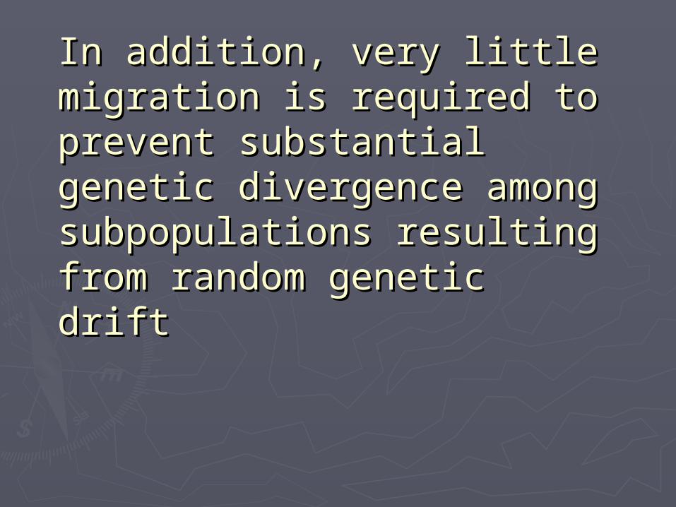
In addition, very little In addition, very little migration is required to migration is required to prevent substantial prevent substantial genetic divergence among genetic divergence among subpopulations resulting subpopulations resulting from random genetic from random genetic driftdrift

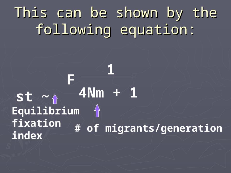
This can be shown by the This can be shown by the following equation:following equation:

Fst ~ 1

4Nm + 1

# of migrants/generation

Equilibriumfixationindex

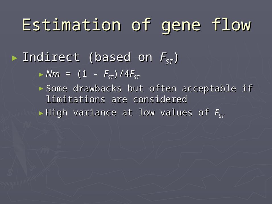
Estimation of gene flowEstimation of gene flow

►Indirect (based on Indirect (based on FFSTST))►NmNm = (1 - = (1 - FFSTST)/4)/4FFSTST

►Some drawbacks but often acceptable if Some drawbacks but often acceptable if limitations are consideredlimitations are considered

►High variance at low values of High variance at low values of FFSTST

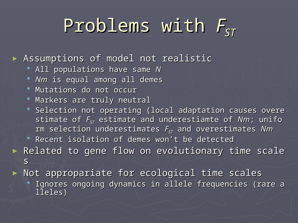
Problems with Problems with FFSTST

► Assumptions of model not realisticAssumptions of model not realistic All populations have same All populations have same NN NmNm is equal among all demes is equal among all demes Mutations do not occurMutations do not occur Markers are truly neutralMarkers are truly neutral Selection not operating (local adaptation causes overestimaSelection not operating (local adaptation causes overestima

te of te of FFSTST estimate and underestiamte of estimate and underestiamte of NmNm; uniform selectio; uniform selection underestimates n underestimates FFSTST and overestimates and overestimates NmNm

Recent isolation of demes won’t be detectedRecent isolation of demes won’t be detected► Related to gene flow on evolutionary time scalesRelated to gene flow on evolutionary time scales► Not appropariate for ecological time scalesNot appropariate for ecological time scales

Ignores ongoing dynamics in allele frequencies (rare alleleIgnores ongoing dynamics in allele frequencies (rare alleles)s)

► Best in situations where Best in situations where Spatial scale small (island model holds and spatiSpatial scale small (island model holds and spatially varying selection unlikely)ally varying selection unlikely)

Migration rates high (rapid attainment of genetic Migration rates high (rapid attainment of genetic equilibrium)equilibrium)

Sample sizes and number of loci used are large - Sample sizes and number of loci used are large - accuracy of estimates accuracy of estimates

Long-term estimate of NLong-term estimate of Neem “averaged” over many gm “averaged” over many generations desiredenerations desired

Not useful for short-term nonequilibrium situatioNot useful for short-term nonequilibrium situations e.g. recently fragmented, rapidly declining pons e.g. recently fragmented, rapidly declining populationspulations

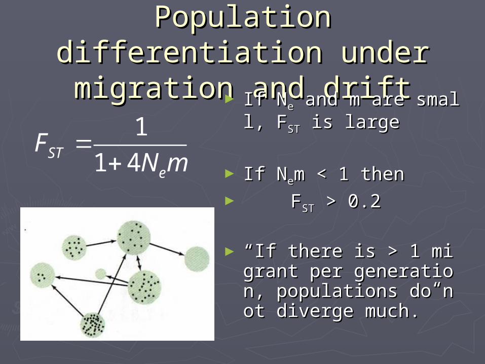
Population Population differentiation under differentiation under migration and driftmigration and drift► If NIf Nee and m are small, and m are small,

FFSTST is large is large

► If NIf Neem < 1 then m < 1 then ► FFSTST > 0.2 > 0.2

►““If there is > 1 migraIf there is > 1 migrant per generation, popunt per generation, populations do not diverge lations do not diverge much.” much.”

1

1 4STe

FN m

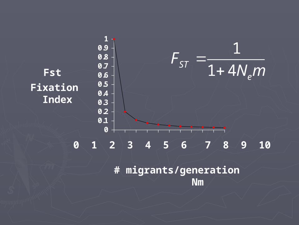
00.10.20.30.40.50.60.70.80.9

1

0 1 2 3 4 5 6 7 8 9 10

Fixation Index

Fst

# migrants/generation Nm

1

1 4STe

FN m

=+

OMPGOMPG rule of thumb rule of thumb

►From this analysis emerged a From this analysis emerged a genetic rule of thumb that genetic rule of thumb that oone ne mmigrant individual per local igrant individual per local population population pper er ggeneration (eneration (OMPGOMPG) ) is sufficient to obscure any is sufficient to obscure any disruptive effects of drift.disruptive effects of drift.

Biologists concerned with pBiologists concerned with population insularization caopulation insularization caused by habitat fragmentatiused by habitat fragmentation began advocating the appon began advocating the application of this principle lication of this principle for conservation purposesfor conservation purposes

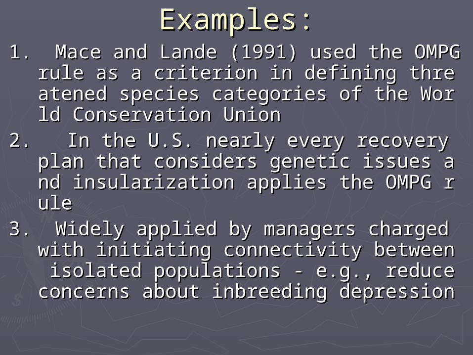
Examples:Examples:1. Mace and Lande (1991) used the OMPG rul1. Mace and Lande (1991) used the OMPG rul

e as a criterion in defining threatened e as a criterion in defining threatened species categories of the World Conservaspecies categories of the World Conservation Uniontion Union

2. In the U.S. nearly every recovery plan 2. In the U.S. nearly every recovery plan that considers genetic issues and insulathat considers genetic issues and insularization applies the OMPG rulerization applies the OMPG rule

3. Widely applied by managers charged with 3. Widely applied by managers charged with initiating connectivity between isolateinitiating connectivity between isolated populations - e.g., reduce concerns abd populations - e.g., reduce concerns about inbreeding depressionout inbreeding depression

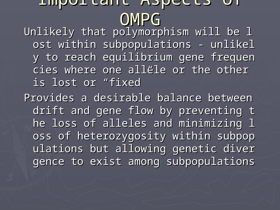
Important Aspects of Important Aspects of OMPGOMPG

Unlikely that polymorphism will be losUnlikely that polymorphism will be lost within subpopulations - unlikely tt within subpopulations - unlikely to reach equilibrium gene frequencies o reach equilibrium gene frequencies where one allele or the other is loswhere one allele or the other is lost or “fixed”t or “fixed”Provides a desirable balance between dProvides a desirable balance between drift and gene flow by preventing the rift and gene flow by preventing the loss of alleles and minimizing loss loss of alleles and minimizing loss of heterozygosity within subpopulatiof heterozygosity within subpopulations but allowing genetic divergence ons but allowing genetic divergence to exist among subpopulationsto exist among subpopulations

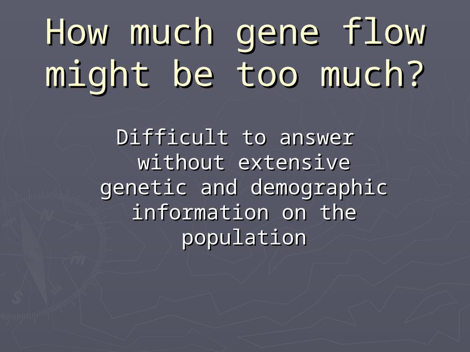
How much gene flow How much gene flow might be too much?might be too much?

Difficult to answer Difficult to answer without extensive without extensive

genetic and demographic genetic and demographic information on the information on the

populationpopulation

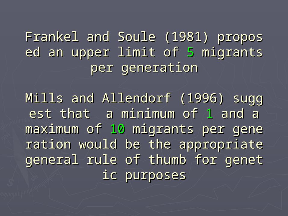
Frankel and Soule (1981) proposed an Frankel and Soule (1981) proposed an upper limit of upper limit of 55 migrants per generat migrants per generat

ionion

Mills and Allendorf (1996) suggest thMills and Allendorf (1996) suggest that a minimum of at a minimum of 11 and a maximum of and a maximum of 1100 migrants per generation would be th migrants per generation would be the appropriate general rule of thumb fe appropriate general rule of thumb f

or genetic purposesor genetic purposes

00.10.20.30.40.50.60.70.80.9

1

0 1 2 3 4 5 6 7 8 9 10

Fixation Index

Fst

# mutation/generation Nu

1

1 4STe

FN

=+

Mutation Mutation has the same effect has the same effect

常用软件常用软件

►Arlequin 3.01Arlequin 3.01 http://anthro.unige.ch/software/arlequin/http://anthro.unige.ch/software/arlequin/

练习练习►利用利用 HapMapHapMap 数据进行群体结构分析；数据进行群体结构分析；

http://www.hapmap.orghttp://www.hapmap.org