Embed Size (px)
Citation preview
因子分析,共分散構造分析Factor Analysis
Structural Equations Model
第 16 章 因子分析 Factor Analysis
主成分分析 Principal Components
第 17 章 共分散構造分析 Structural Equations Model (SEM)
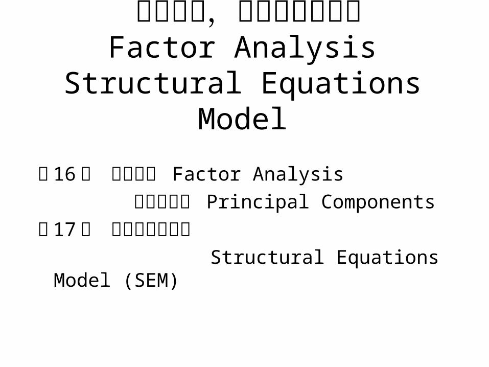
線形構造の図式(p 310 )Linear Structure
観測変数Observed V.
潜在変数Latent V.
誤差項Error term
重回帰分析 Multiple Linear Regression( 複数の観測変数と誤差で目的の観測変数を表現 )
y
x 1
x2e
因子分析 Factor Analysis( 複数の観測変数を共通の潜在変数で表現 )
y1
y2
y3
f1
f2
e1
e2
e3
主成分分析 Principal Components( 複数の観測変数を統合し集約した潜在変数で表現 )
x1
x2
x3
h1
h2
e1
e2
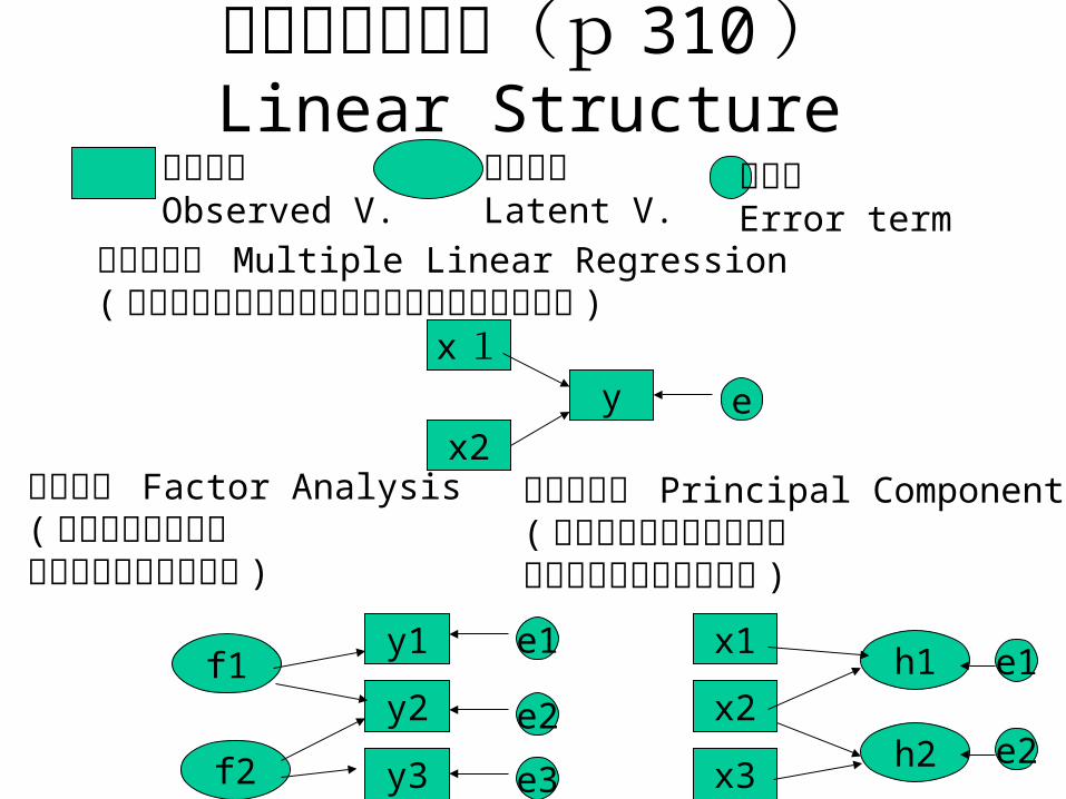
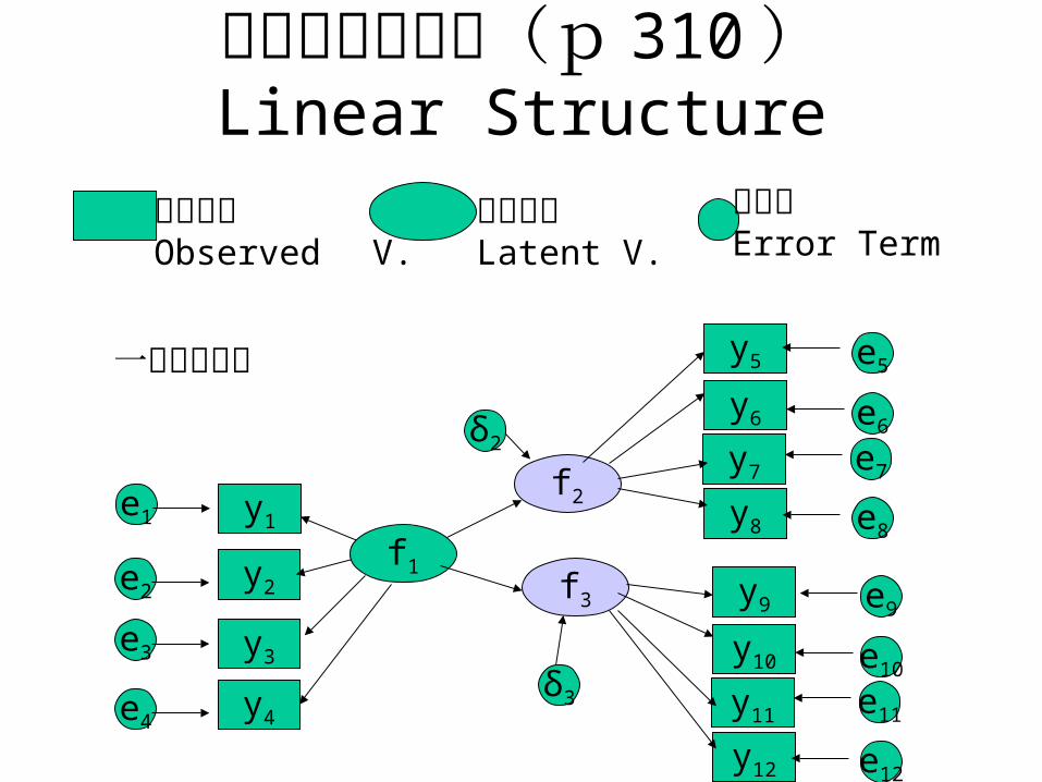
線形構造の図式(p 310 )Linear Structure
観測変数Observed V.
潜在変数Latent V.
誤差項Error term
一般線形構造General Structure
y4
y5
e4y1
y2
y3
f2
f3
e1
e2
e3e5
f1
δ3
δ2
Structural Equation Model (SEM), Linear Structure Regression with Latent variables(LISREL)
線形構造の図式(p 310 )Linear Structure
観測変数Observed V.
潜在変数Latent V.
誤差項Error Term
一般線形構造
y1
y2
e1
y7
y8
f2
f3
e7
e8
e2
f1
δ3
δ2
y3
y4
e3
e4
y5
y6
e5
e6
y11
y12
e11
e12
y9
y10
e9
e10
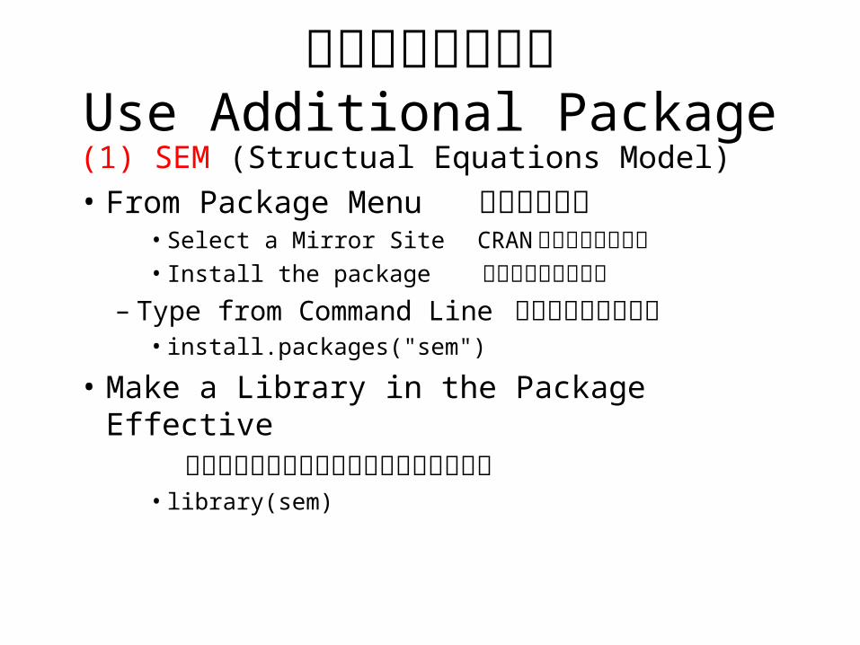
パッケージを使うUse Additional Package
(1) SEM (Structual Equations Model)
• From Package Menu メニューから• Select a Mirror Site CRAN ミラーサイト指定• Install the package プルダウンから選ぶ
– Type from Command Line コマンドラインから• install.packages("sem")
• Make a Library in the Package Effective パッケージ内のライブラリーを有効にする
• library(sem)
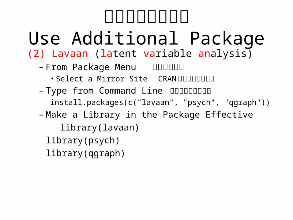
パッケージを使うUse Additional Package
(2) Lavaan (latent variable analysis)– From Package Menu メニューから
• Select a Mirror Site CRAN ミラーサイト指定– Type from Command Line コマンドラインから
install.packages(c("lavaan", "psych", "qgraph"))
– Make a Library in the Package Effective
library(lavaan)
library(psych)
library(qgraph)
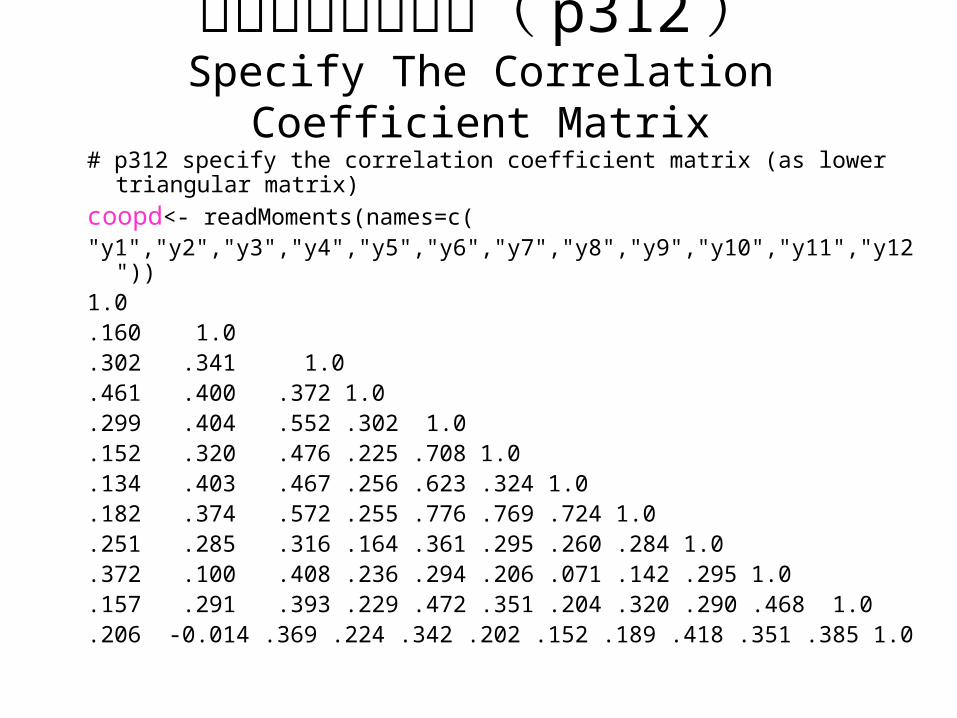
相関係数行列入力( p312 )Specify The Correlation Coefficient Matrix
# p312 specify the correlation coefficient matrix (as lower triangular matrix)
coopd<- readMoments(names=c("y1","y2","y3","y4","y5","y6","y7","y8","y9","y10","y11","y12"))1.0.160 1.0.302 .341 1.0.461 .400 .372 1.0.299 .404 .552 .302 1.0.152 .320 .476 .225 .708 1.0.134 .403 .467 .256 .623 .324 1.0.182 .374 .572 .255 .776 .769 .724 1.0.251 .285 .316 .164 .361 .295 .260 .284 1.0.372 .100 .408 .236 .294 .206 .071 .142 .295 1.0.157 .291 .393 .229 .472 .351 .204 .320 .290 .468 1.0.206 -0.014 .369 .224 .342 .202 .152 .189 .418 .351 .385 1.0
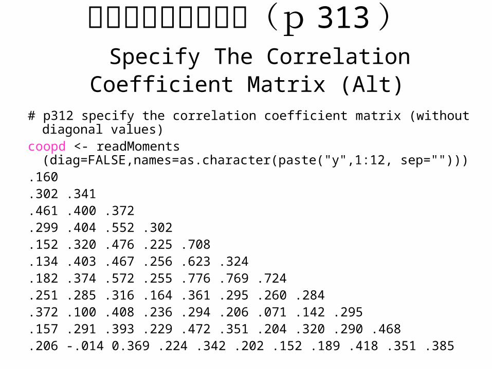
相関係数行列の入力(p 313 ) Specify The Correlation Coefficient Matrix (Alt)
# p312 specify the correlation coefficient matrix (without diagonal values)coopd <- readMoments (diag=FALSE,names=as.character(paste("y",1:12,
sep=""))).160 .302 .341 .461 .400 .372.299 .404 .552 .302.152 .320 .476 .225 .708.134 .403 .467 .256 .623 .324.182 .374 .572 .255 .776 .769 .724.251 .285 .316 .164 .361 .295 .260 .284.372 .100 .408 .236 .294 .206 .071 .142 .295.157 .291 .393 .229 .472 .351 .204 .320 .290 .468.206 -.014 0.369 .224 .342 .202 .152 .189 .418 .351 .385
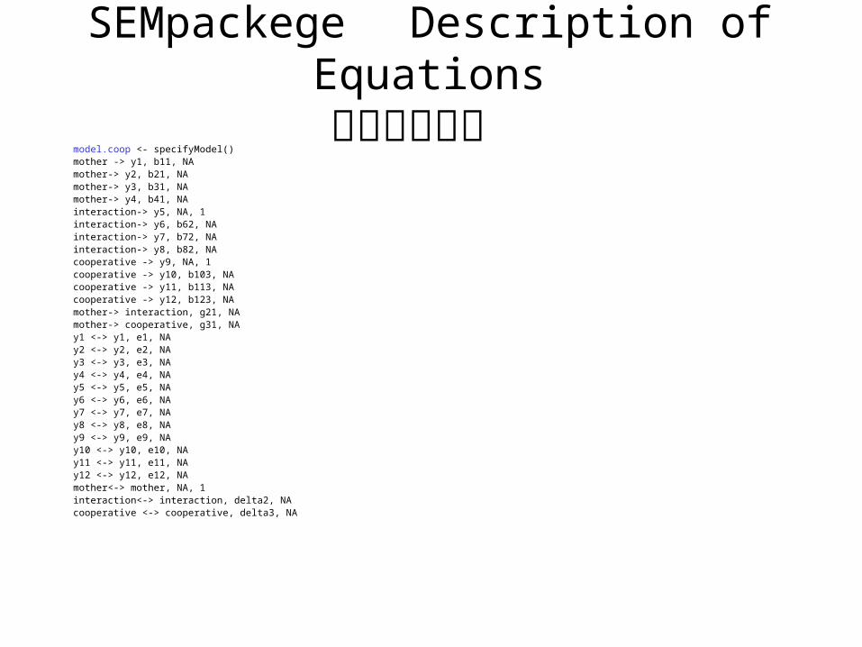
SEMpackege Description of Equations方程式の記述
model.coop <- specifyModel()mother -> y1, b11, NAmother-> y2, b21, NAmother-> y3, b31, NAmother-> y4, b41, NAinteraction-> y5, NA, 1interaction-> y6, b62, NAinteraction-> y7, b72, NAinteraction-> y8, b82, NAcooperative -> y9, NA, 1cooperative -> y10, b103, NAcooperative -> y11, b113, NAcooperative -> y12, b123, NAmother-> interaction, g21, NAmother-> cooperative, g31, NAy1 <-> y1, e1, NAy2 <-> y2, e2, NAy3 <-> y3, e3, NAy4 <-> y4, e4, NAy5 <-> y5, e5, NAy6 <-> y6, e6, NAy7 <-> y7, e7, NAy8 <-> y8, e8, NAy9 <-> y9, e9, NAy10 <-> y10, e10, NAy11 <-> y11, e11, NAy12 <-> y12, e12, NAmother<-> mother, NA, 1interaction<-> interaction, delta2, NAcooperative <-> cooperative, delta3, NA
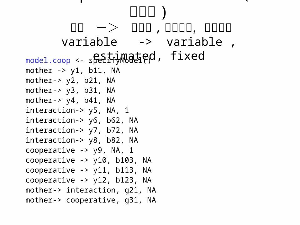
Description of Relations( 係数の記述 )変数 -> 影響先 , 推定母数,固定母数
variable -> variable , estimated, fixed
model.coop <- specifyModel()mother -> y1, b11, NAmother-> y2, b21, NAmother-> y3, b31, NAmother-> y4, b41, NAinteraction-> y5, NA, 1interaction-> y6, b62, NAinteraction-> y7, b72, NAinteraction-> y8, b82, NAcooperative -> y9, NA, 1cooperative -> y10, b103, NAcooperative -> y11, b113, NAcooperative -> y12, b123, NAmother-> interaction, g21, NAmother-> cooperative, g31, NA
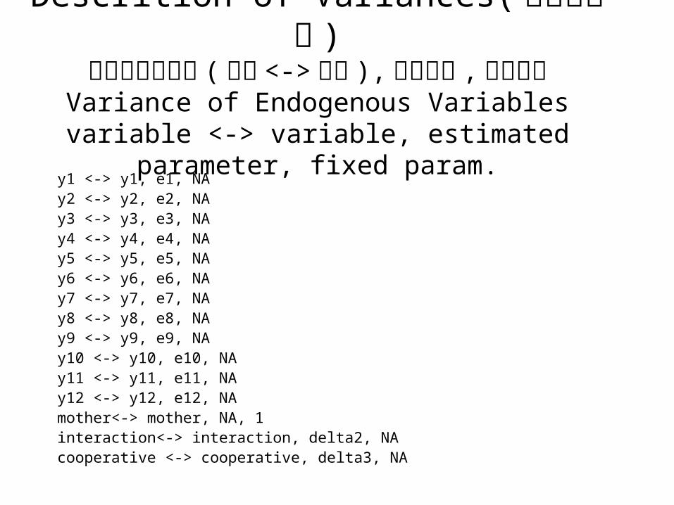
Descrition of Variances( 分散の記述 )内生変数の分散 ( 変数 <-> 変数 ), 推定母数 , 固定母
数Variance of Endogenous Variables
variable <-> variable, estimated parameter, fixed param.y1 <-> y1, e1, NAy2 <-> y2, e2, NAy3 <-> y3, e3, NAy4 <-> y4, e4, NAy5 <-> y5, e5, NAy6 <-> y6, e6, NAy7 <-> y7, e7, NAy8 <-> y8, e8, NAy9 <-> y9, e9, NAy10 <-> y10, e10, NAy11 <-> y11, e11, NAy12 <-> y12, e12, NAmother<-> mother, NA, 1interaction<-> interaction, delta2, NAcooperative <-> cooperative, delta3, NA
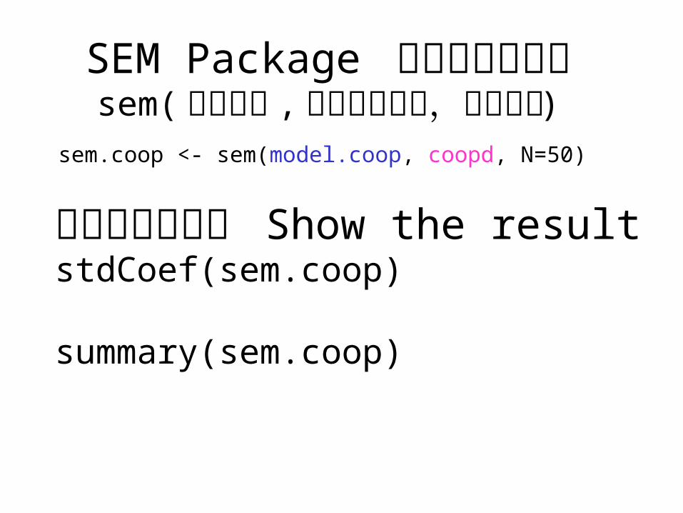
SEM Package 推定母数の計算sem( モデル名 , 相関係数行列,データ
数 )sem.coop <- sem(model.coop, coopd, N=50)
推定結果の表示 Show the resultstdCoef(sem.coop)
summary(sem.coop)
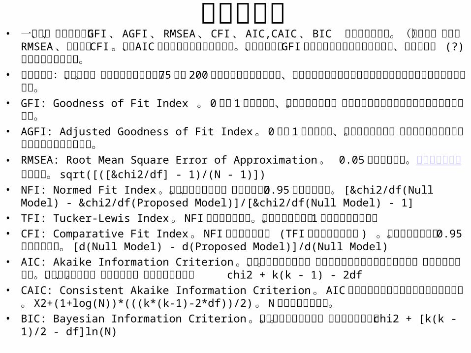
適合度指標• 一般に、カイ二乗値、 GFI 、 AGFI 、 RMSEA 、 CFI 、 AIC,CAIC 、 BIC などが使われる
。(たぶん)まずは RMSEA 、それから CFI 。で、 AIC でほかのモデルと比較する。カイ二乗値、 GFI 系はいろいろよくないらしいが、慣習として (?) 報告だけはしておく。
• カイ二乗値:小さくて、有意じゃないとよい。 75 から 200 ケースくらいならよいが、それ以上になると常に有意になってしまうのでよろしくない指標。
• GFI: Goodness of Fit Index 。 0 から 1 までの値で、大きいほどよい。サンプルサイズに依存するのでおすすめしない。
• AGFI: Adjusted Goodness of Fit Index 。 0 から 1 までの値で、大きいほどよい。サンプルサイズに依存するのでおすすめしない。
• RMSEA: Root Mean Square Error of Approximation 。 0.05 以下だとよい。信頼区間の計算を薦める。 sqrt([([&chi2/df] - 1)/(N - 1)])
• NFI: Normed Fit Index 。ヌルモデルとの差。大きいほど、 0.95 以上だとよい。 [&chi2/df(Null Model) - &chi2/df(Proposed Model)]/[&chi2/df(Null Model) - 1]
• TFI: Tucker-Lewis Index 。 NFI を自由度で補正。大きいほどよい。 1 を超えることもある• CFI: Comparative Fit Index 。 NFI を自由度で補正 (TFI とは違うやりかた ) 。大きいほどよい
。 0.95 以上だとよい。 [d(Null Model) - d(Proposed Model)]/d(Null Model)• AIC: Akaike Information Criterion 。カイ二乗値に自由度、パラメータ数の補正を加えたもの
。小さいほうがよい。相対基準なので、いくつ以下、というのはない。 chi2 + k(k - 1) - 2df• CAIC: Consistent Akaike Information Criterion 。 AIC のサンプルサイズの補正をさらに加えた
。 X2+(1+log(N))*(((k*(k-1)-2*df))/2) 。 N はサンプルサイズ。• BIC: Bayesian Information Criterion 。事後の分布との比較。小さいほどよい。 chi2 + [k(k - 1)/2
- df]ln(N)
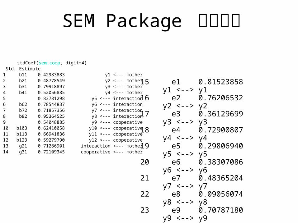
SEM Package 標準化解
stdCoef(sem.coop, digit=4) Std. Estimate 1 b11 0.42983883 y1 <--- mother2 b21 0.48778549 y2 <--- mother3 b31 0.79918897 y3 <--- mother4 b41 0.52056885 y4 <--- mother5 0.83781298 y5 <--- interaction6 b62 0.78544837 y6 <--- interaction7 b72 0.71857356 y7 <--- interaction8 b82 0.95364525 y8 <--- interaction9 0.54048885 y9 <--- cooperative10 b103 0.62410058 y10 <--- cooperative11 b113 0.66941836 y11 <--- cooperative12 b123 0.59279790 y12 <--- cooperative13 g21 0.71286901 interaction <--- mother14 g31 0.72109345 cooperative <--- mother
15 e1 0.81523858 y1 <--> y116 e2 0.76206532 y2 <--> y217 e3 0.36129699 y3 <--> y318 e4 0.72900807 y4 <--> y419 e5 0.29806940 y5 <--> y520 e6 0.38307086 y6 <--> y621 e7 0.48365204 y7 <--> y722 e8 0.09056074 y8 <--> y823 e9 0.70787180 y9 <--> y924 e10 0.61049846 y10 <--> y1025 e11 0.55187906 y11 <--> y1126 e12 0.64859064 y12 <--> y1227 1.00000000 mother <--> mother28 delta2 0.49181777 interaction <--> interaction29 delta3 0.48002423 cooperative <--> cooperative
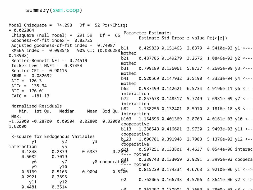
summary(sem.coop)
Model Chisquare = 74.298 Df = 52 Pr(>Chisq) = 0.022864 Chisquare (null model) = 291.59 Df = 66 Goodness-of-fit index = 0.82725 Adjusted goodness-of-fit index = 0.74087 RMSEA index = 0.093548 90% CI: (0.036288, 0.13902) Bentler-Bonnett NFI = 0.74519 Tucker-Lewis NNFI = 0.87454 Bentler CFI = 0.90115 SRMR = 0.082692 AIC = 126.3 AICc = 135.34 BIC = 176.01 CAIC = -181.13
Normalized Residuals Min. 1st Qu. Median Mean 3rd Qu. Max. -1.52000 -0.28700 0.00504 0.02800 0.32000 1.62000
R-square for Endogenous Variables y1 y2 y3 y4 interaction y5 0.1848 0.2379 0.6387 0.2710 0.5082 0.7019 y6 y7 y8 cooperative y9 y10 0.6169 0.5163 0.9094 0.5200 0.2921 0.3895 y11 y12 0.4481 0.3514
Parameter Estimates Estimate Std Error z value Pr(>|z|) b11 0.429839 0.151463 2.8379 4.5410e-03 y1 <--- mother b21 0.487785 0.149279 3.2676 1.0846e-03 y2 <--- mother b31 0.799189 0.136061 5.8737 4.2605e-09 y3 <--- mother b41 0.520569 0.147932 3.5190 4.3323e-04 y4 <--- mother b62 0.937499 0.142621 6.5734 4.9196e-11 y6 <--- interaction b72 0.857678 0.148517 5.7749 7.6981e-09 y7 <--- interaction b82 1.138256 0.132401 8.5970 8.1816e-18 y8 <--- interaction b103 1.154696 0.401369 2.8769 4.0161e-03 y10 <--- cooperative b113 1.238543 0.416601 2.9730 2.9493e-03 y11 <--- cooperative b123 1.096781 0.391948 2.7983 5.1376e-03 y12 <--- cooperative g21 0.597251 0.133801 4.4637 8.0544e-06 interaction <--- mother g31 0.389743 0.133059 2.9291 3.3995e-03 cooperative <--- mother e1 0.815239 0.174334 4.6763 2.9210e-06 y1 <--> y1 e2 0.762065 0.166733 4.5706 4.8641e-06 y2 <--> y2 e3 0.361297 0.130904 2.7600 5.7800e-03 y3 <--> y3 e4 0.729008 0.162139 4.4962 6.9182e-06 y4 <--> y4 e5 0.298069 0.074691 3.9907 6.5882e-05 y5 <--> y5 e6 0.383071 0.088169 4.3447 1.3944e-05 y6 <--> y6 e7 0.483652 0.105790 4.5718 4.8350e-06 y7 <--> y7 e8 0.090561 0.055202 1.6405 1.0090e-01 y8 <--> y8 e9 0.707872 0.165572 4.2753 1.9087e-05 y9 <--> y9 e10 0.610498 0.156681 3.8965 9.7612e-05 y10 <--> y10 e11 0.551879 0.153089 3.6050 3.1220e-04 y11 <--> y11 e12 0.648591 0.159798 4.0588 4.9324e-05 y12 <--> y12 delta2 0.345222 0.120587 2.8628 4.1986e-03 interaction <--> interactiondelta3 0.140229 0.092747 1.5120 1.3055e-01 cooperative <--> cooperative
Iterations = 48
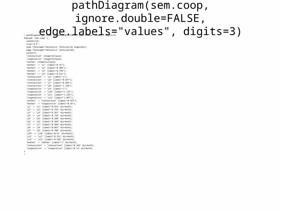
pathDiagram(sem.coop, ignore.double=FALSE, edge.labels="values", digits=3)
> pathDiagram(sem.coop, ignore.double=FALSE, edge.labels="values", digits=3)
digraph "sem.coop" {
rankdir=LR;
size="8,8";
node [fontname="Helvetica" fontsize=14 shape=box];
edge [fontname="Helvetica" fontsize=10];
center=1;
"interaction" [shape=ellipse]
"cooperative" [shape=ellipse]
"mother" [shape=ellipse]
"mother" -> "y1" [label="0.43"];
"mother" -> "y2" [label="0.488"];
"mother" -> "y3" [label="0.799"];
"mother" -> "y4" [label="0.521"];
"interaction" -> "y5" [label="1"];
"interaction" -> "y6" [label="0.937"];
"interaction" -> "y7" [label="0.858"];
"interaction" -> "y8" [label="1.138"];
"cooperative" -> "y9" [label="1"];
"cooperative" -> "y10" [label="1.155"];
"cooperative" -> "y11" [label="1.239"];
"cooperative" -> "y12" [label="1.097"];
"mother" -> "interaction" [label="0.597"];
"mother" -> "cooperative" [label="0.39"];
"y1" -> "y1" [label="0.815" dir=both];
"y2" -> "y2" [label="0.762" dir=both];
"y3" -> "y3" [label="0.361" dir=both];
"y4" -> "y4" [label="0.729" dir=both];
"y5" -> "y5" [label="0.298" dir=both];
"y6" -> "y6" [label="0.383" dir=both];
"y7" -> "y7" [label="0.484" dir=both];
"y8" -> "y8" [label="0.091" dir=both];
"y9" -> "y9" [label="0.708" dir=both];
"y10" -> "y10" [label="0.61" dir=both];
"y11" -> "y11" [label="0.552" dir=both];
"y12" -> "y12" [label="0.649" dir=both];
"mother" -> "mother" [label="1" dir=both];
"interaction" -> "interaction" [label="0.345" dir=both];
"cooperative" -> "cooperative" [label="0.14" dir=both];
}
>
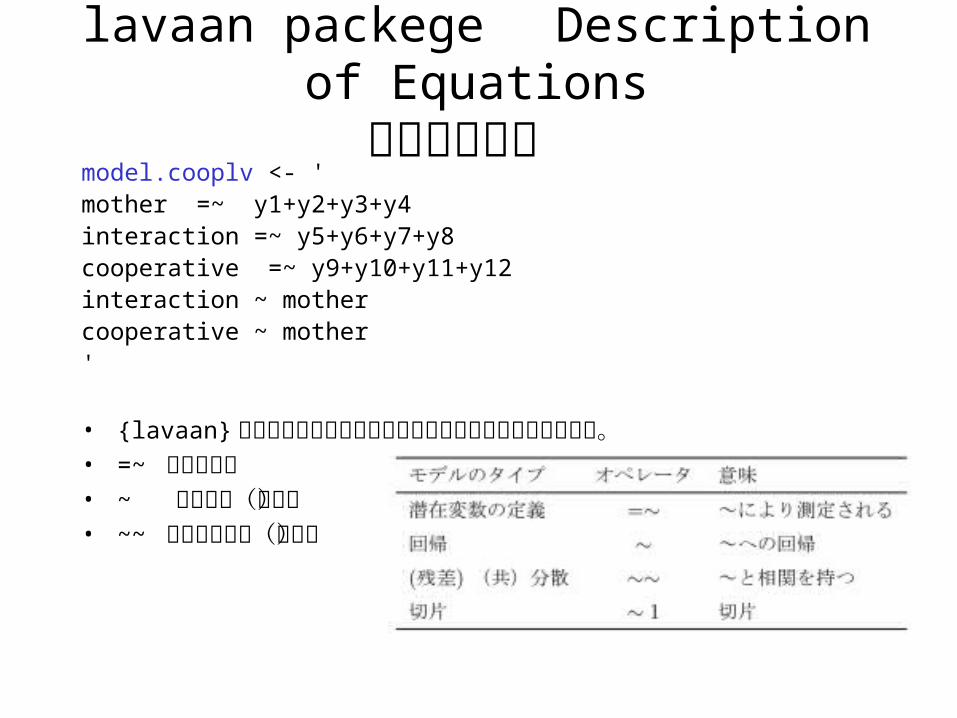
lavaan packege Description of Equations方程式の記述
model.cooplv <- 'mother =~ y1+y2+y3+y4interaction =~ y5+y6+y7+y8cooperative =~ y9+y10+y11+y12interaction ~ mothercooperative ~ mother '
• {lavaan} パッケージでは以下のような記号の使い方をしています。• =~ 測定方程式• ~ 構造程式(回帰)• ~~ 残差の共分散(相関)
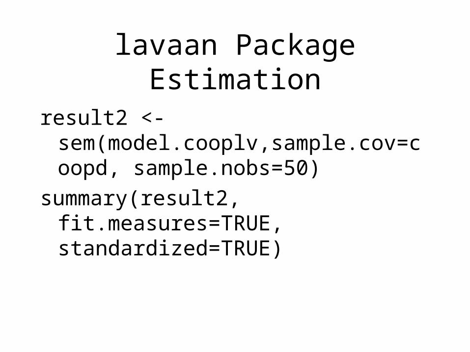
lavaan Package Estimation
result2 <- sem(model.cooplv,sample.cov=coopd, sample.nobs=50)
summary(result2, fit.measures=TRUE, standardized=TRUE)
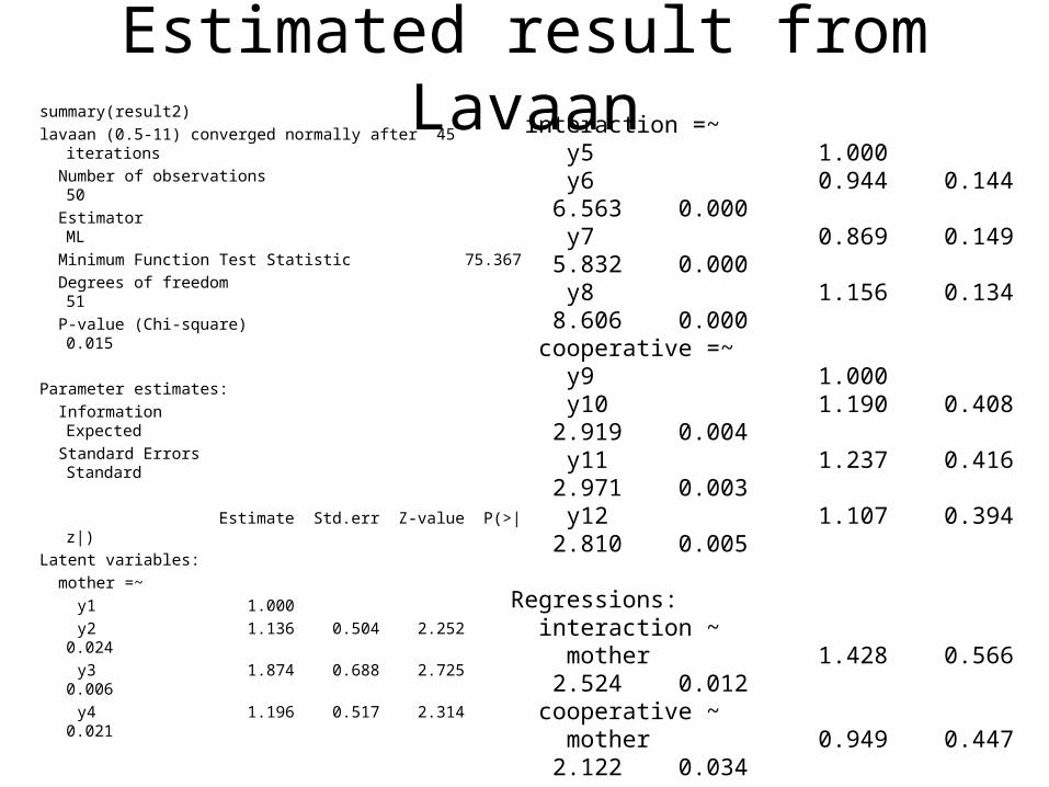
Estimated result from Lavaansummary(result2)
lavaan (0.5-11) converged normally after 45 iterations
Number of observations 50
Estimator ML
Minimum Function Test Statistic 75.367
Degrees of freedom 51
P-value (Chi-square) 0.015
Parameter estimates:
Information Expected
Standard Errors Standard
Estimate Std.err Z-value P(>|z|)
Latent variables:
mother =~
y1 1.000
y2 1.136 0.504 2.252 0.024
y3 1.874 0.688 2.725 0.006
y4 1.196 0.517 2.314 0.021
interaction =~ y5 1.000 y6 0.944 0.144 6.563 0.000 y7 0.869 0.149 5.832 0.000 y8 1.156 0.134 8.606 0.000 cooperative =~ y9 1.000 y10 1.190 0.408 2.919 0.004 y11 1.237 0.416 2.971 0.003 y12 1.107 0.394 2.810 0.005
Regressions: interaction ~ mother 1.428 0.566 2.524 0.012 cooperative ~ mother 0.949 0.447 2.122 0.034
Covariances: interaction ~~ cooperative -0.041 0.060 -0.675 0.499
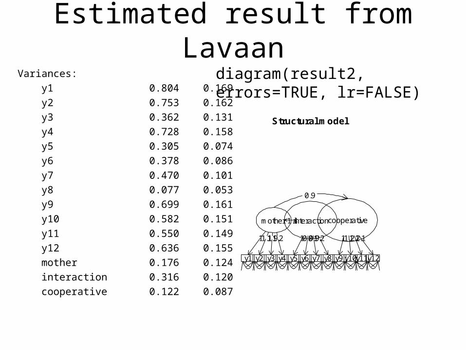
Estimated result from LavaanVariances:
y1 0.804 0.169
y2 0.753 0.162
y3 0.362 0.131
y4 0.728 0.158
y5 0.305 0.074
y6 0.378 0.086
y7 0.470 0.101
y8 0.077 0.053
y9 0.699 0.161
y10 0.582 0.151
y11 0.550 0.149
y12 0.636 0.155
mother 0.176 0.124
interaction 0.316 0.120
cooperative 0.122 0.087
diagram(result2, errors=TRUE, lr=FALSE)
Structural model
y1 y2 y3 y4 y5 y6 y7 y8 y9 y10y11y12
mother
11.11.91.2
interaction
10.90.91.2
cooperative
11.21.21.1
1.4
0.9
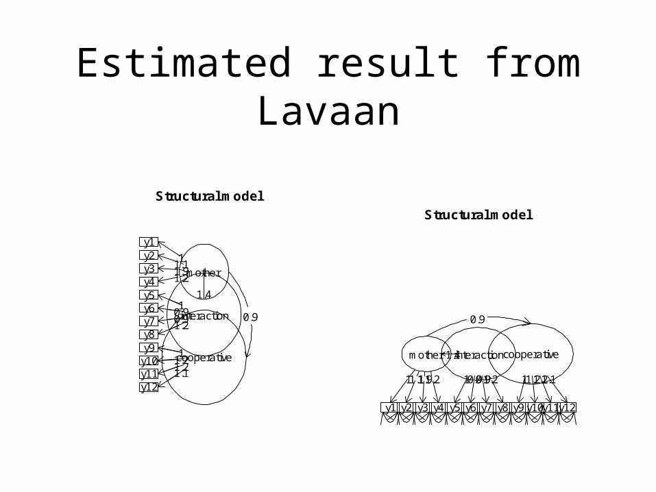
Estimated result from Lavaan
Structural model
y1 y2 y3 y4 y5 y6 y7 y8 y9 y10y11y12
mother
11.11.91.2
interaction
10.90.91.2
cooperative
11.21.21.1
1.4
0.9
Structural model
y1y2y3y4y5y6y7y8y9y10y11y12
mother11.11.91.2
interaction10.90.91.2
cooperative11.21.21.1
1.4
0.9