* Greatest Hits: Old songs from an old performer No covers of others’ work.

Unit Roots Greatest Hits *

David A. Dickey – NC State University

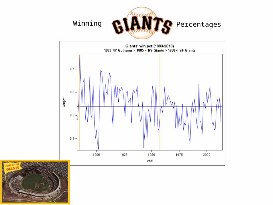
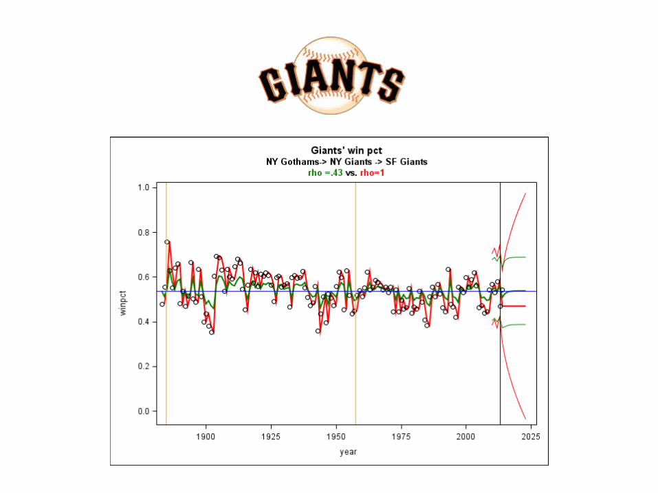
Winning Percentages

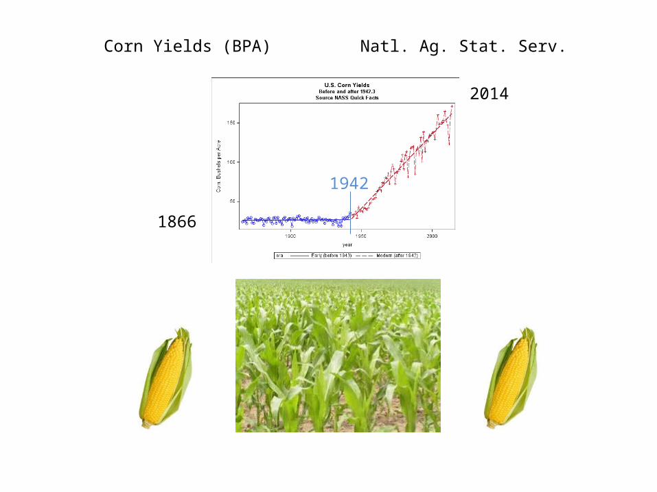
1866

2014

Corn Yields (BPA) Natl. Ag. Stat. Serv.

1942

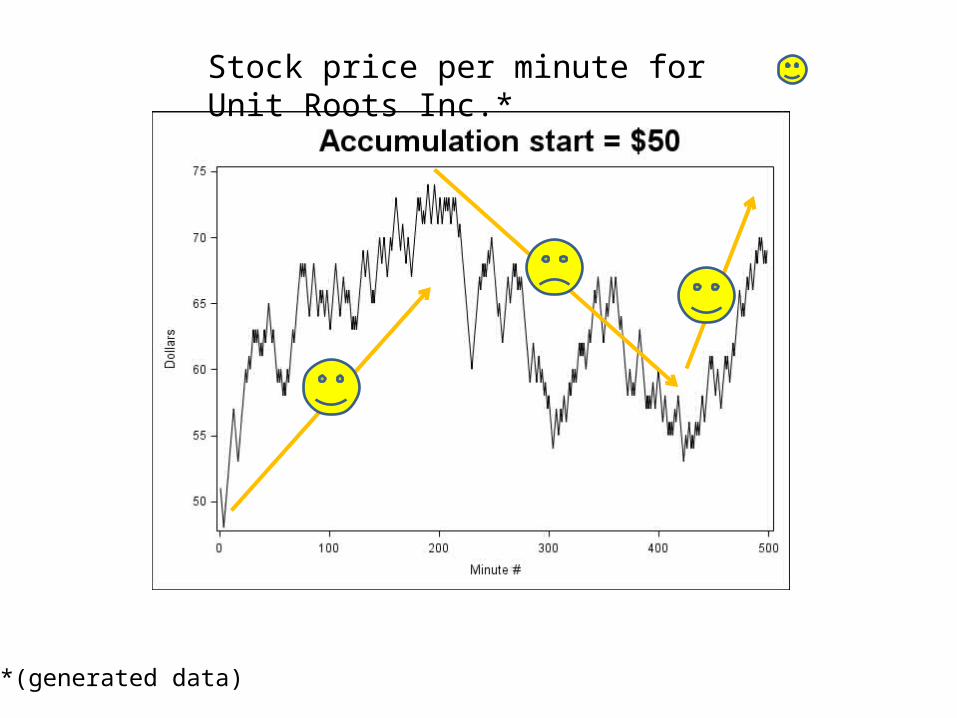
Stock price per minute for Unit Roots Inc.*

*(generated data)

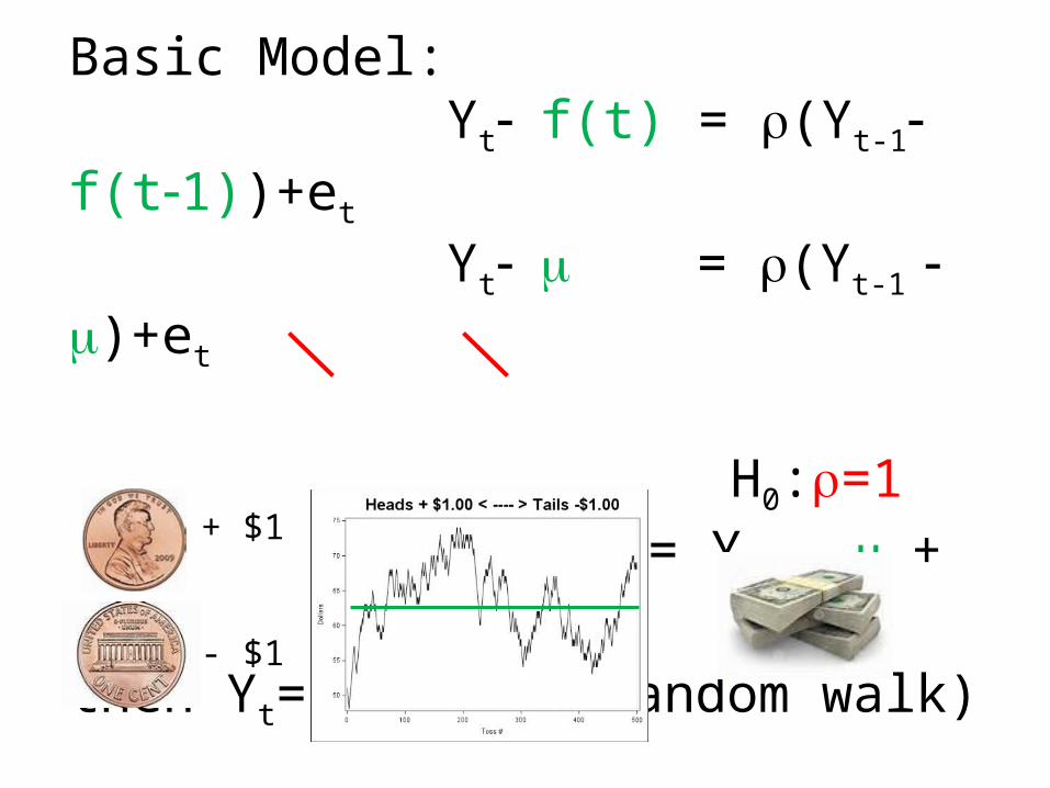
Basic Model: Yt- f(t) = r(Yt-1- f(t-1))+et

Yt- m = r(Yt-1 - m)+et

H0:r=1 Yt-m = Yt-1- m + et

then Yt= Yt-1+et (random walk)+ $1

- $1

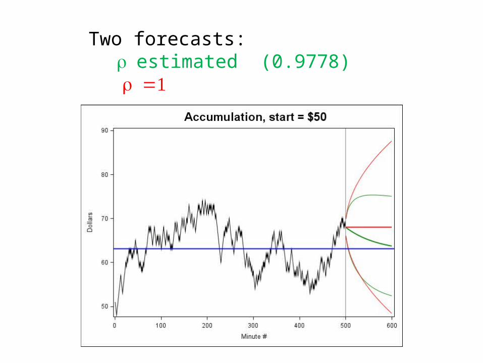
Two forecasts: r estimated (0.9778) =1r

E = MC2

= ?r

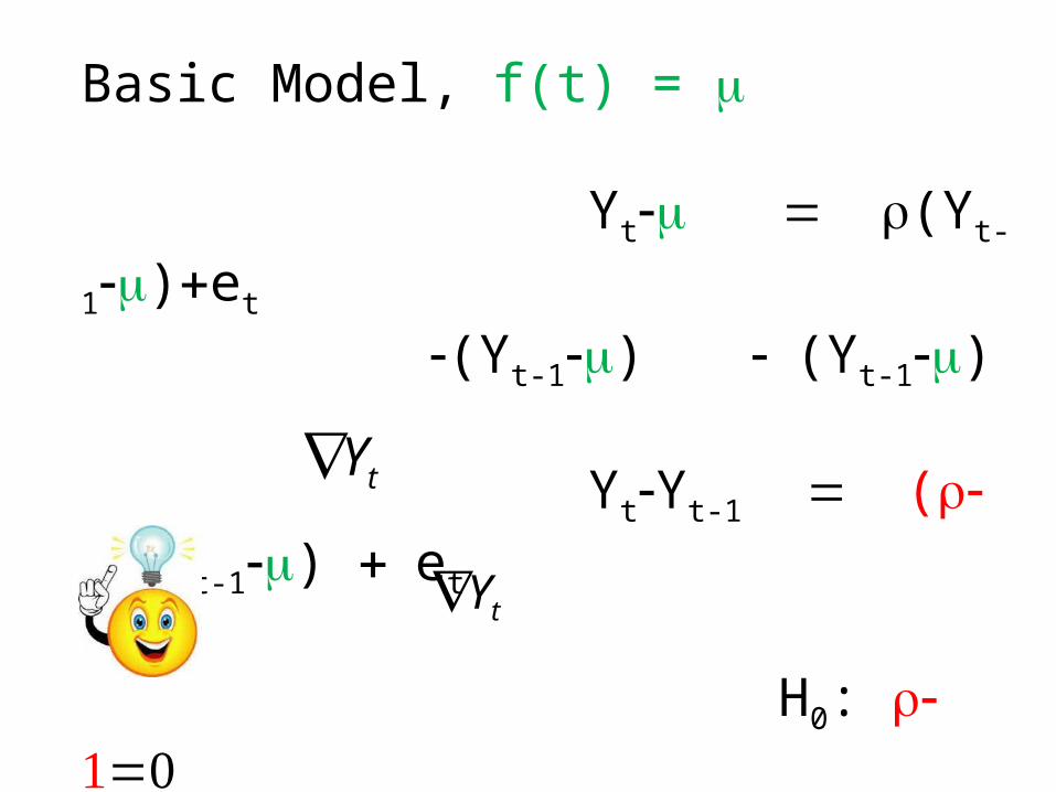
Basic Model, f(t) = m

Yt-m = r(Yt-1-m)+et

-(Yt-1-m) - (Yt-1-m)

Yt-Yt-1 = ( -1)r (Yt-1-m) + et

H0: -1r =0 Regress on 1, Yt-1

t-stat

tY

tY

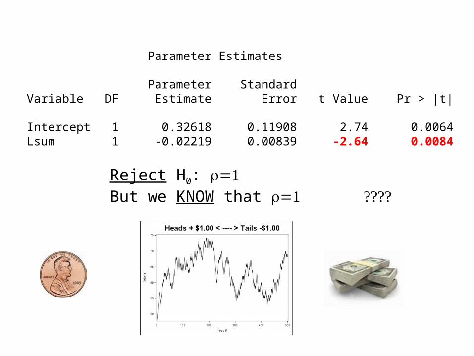
Parameter Estimates

Parameter Standard Variable DF Estimate Error t Value Pr > |t|

Intercept 1 0.32618 0.11908 2.74 0.0064 Lsum 1 -0.02219 0.00839 -2.64 0.0084

Reject H0: =1rBut we KNOW that =1 ????r

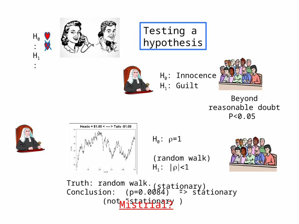
Truth: random walk. Conclusion: (p=0.0084) -> stationary (not “stationary”)

H0:H1:

H0: InnocenceH1: Guilt

Beyond reasonable doubt

P<0.05

H0: r=1 (random walk)H1: | |<r 1 (stationary)

Mistrial?

Testing a hypothesis

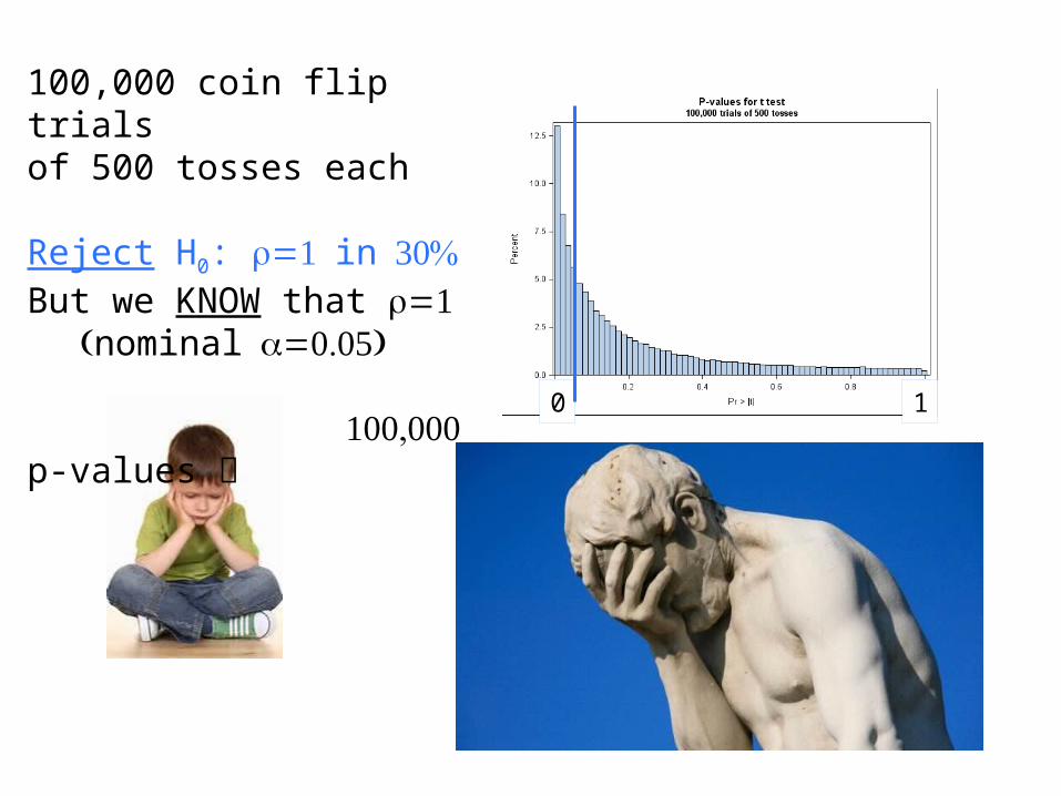
100,000 coin flip trialsof 500 tosses each Reject H0: =1 r in 30%But we KNOW that =1r (nominal =0.05)a

100,000 p-values

0 1

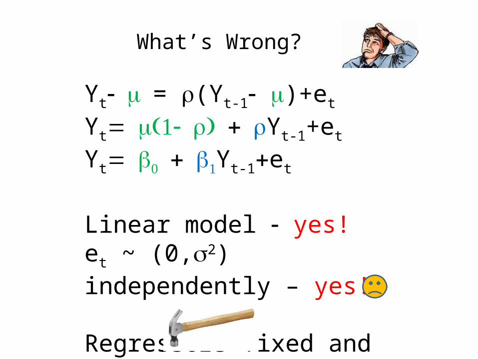
What’s Wrong?

Yt- m = r(Yt-1- m)+et

Yt= (1- )m r + rYt-1+et

Yt= b0 + b1Yt-1+et

Linear model - yes!et ~ (0,s2) independently – yes!

Regressors fixed and known

WilburWright

“I confess that in 1901 I said to my brother Orville that man would not fly for fifty years.” (first flight Dec. 1903)

Lesson 1:

Jim Valvano NCSU basketball coach

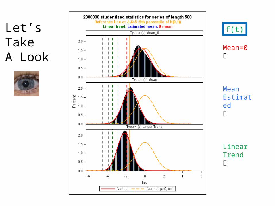
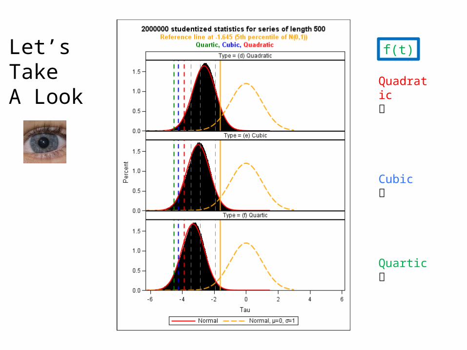
Let’sTake A Look

Mean=0

Mean Estimated

LinearTrend

f(t)

Let’sTake A Look

Quadratic

Cubic

Quartic

f(t)

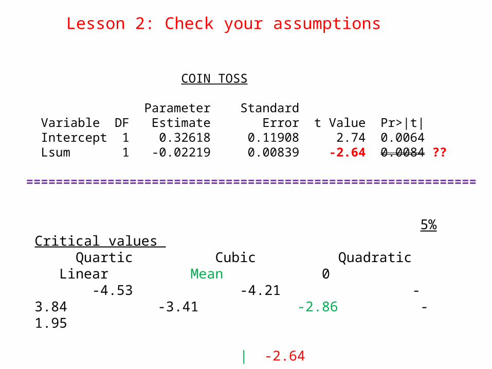
COIN TOSS

Parameter Standard Variable DF Estimate Error t Value Pr>|t| Intercept 1 0.32618 0.11908 2.74 0.0064 Lsum 1 -0.02219 0.00839 -2.64 0.0084 ??

=============================================================

5% Critical values Quartic Cubic Quadratic Linear Mean 0 -4.53 -4.21 -3.84 -3.41 -2.86 -1.95 | -2.64 reject unit roots | don’t reject | | True Pr{t<-2.64} | exceeds 0.05

Lesson 2: Check your assumptions

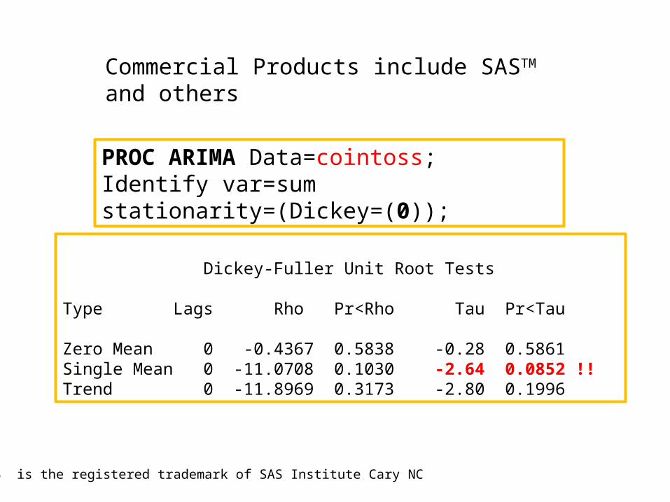
Commercial Products include SASTM and others

Dickey-Fuller Unit Root Tests

Type Lags Rho Pr<Rho Tau Pr<Tau

Zero Mean 0 -0.4367 0.5838 -0.28 0.5861Single Mean 0 -11.0708 0.1030 -2.64 0.0852 !!Trend 0 -11.8969 0.3173 -2.80 0.1996

PROC ARIMA Data=cointoss; Identify var=sum stationarity=(Dickey=(0));

TM SAS is the registered trademark of SAS Institute Cary NC

Where are my clothes?H0: =1r H1:| |<1r

?

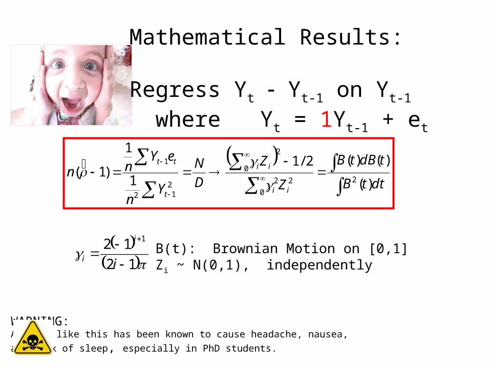
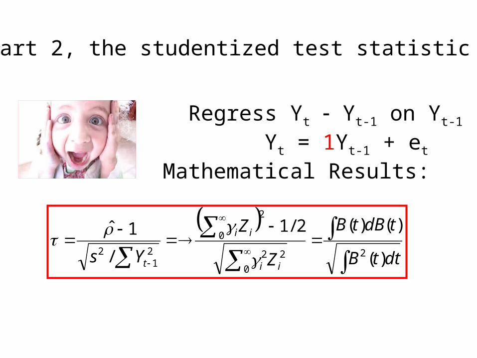
Mathematical Results:

Regress Yt - Yt-1 on Yt-1

where Yt = 1Yt-1 + et

WARNING:Algebra like this has been known to cause headache, nausea, and lack of sleep, especially in PhD students.

dttB

tdBtB

Z

Z

D

N

Yn

eYnn

ii

ii

t

tt

)(

)()(2/1

1

1

)1(2

0

22

2

0

212

1

B(t): Brownian Motion on [0,1]Zi ~ N(0,1), independently

12

12 1

i

i

i

dttB

tdBtB

Z

Z

Ysii

ii

t )(

)()(2/1

/

1ˆ2

0

22

2

0

21

2

Part 2, the studentized test statistic (t)

Regress Yt - Yt-1 on Yt-1

Yt = 1Yt-1 + et

Mathematical Results:

Whether you think you can, or you think you can't--you're right.

Henry Ford

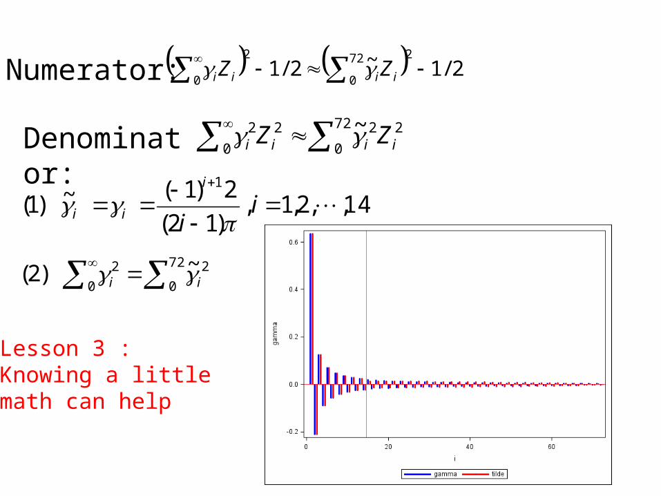
Denominator:

Numerator:

72

0

22

0

22 ~iiii ZZ

72

0

2

0

2 ~)2( ii

14,,2,1,)12(

2)1(~)1(1

ii

i

ii

Lesson 3 :Knowing a little math can help

2/1~2/1272

0

2

0

iiii ZZ

Nice formulas Grandpa!

You can see how excited I am.

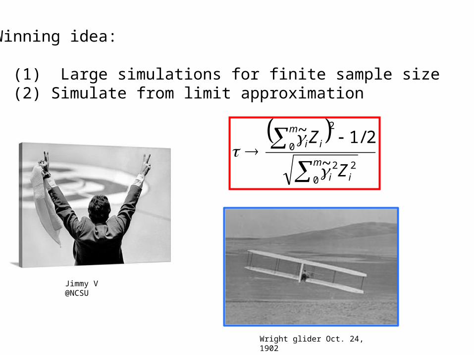
Winning idea:

(1) Large simulations for finite sample size (2) Simulate from limit approximation

m

ii

m

ii

Z

Z

0

22

2

0

~

2/1~

Wright glider Oct. 24, 1902

Jimmy V@NCSU

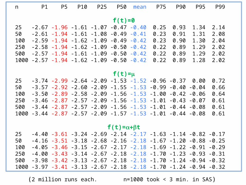
n P1 P5 P10 P25 P50 mean P75 P90 P95 P99

f(t)=0 25 -2.67 -1.96 -1.61 -1.07 -0.47 -0.40 0.25 0.93 1.34 2.14 50 -2.61 -1.94 -1.61 -1.08 -0.49 -0.41 0.23 0.91 1.31 2.08 100 -2.59 -1.94 -1.62 -1.09 -0.49 -0.42 0.23 0.90 1.30 2.04 250 -2.58 -1.94 -1.62 -1.09 -0.50 -0.42 0.22 0.89 1.29 2.02 500 -2.57 -1.94 -1.61 -1.09 -0.50 -0.42 0.22 0.89 1.29 2.02 1000 -2.57 -1.94 -1.62 -1.09 -0.50 -0.42 0.22 0.89 1.28 2.02

f(t)=m 25 -3.74 -2.99 -2.64 -2.09 -1.53 -1.52 -0.96 -0.37 0.00 0.72 50 -3.57 -2.92 -2.60 -2.09 -1.55 -1.53 -0.99 -0.40 -0.04 0.66 100 -3.50 -2.89 -2.58 -2.09 -1.56 -1.53 -1.00 -0.42 -0.06 0.64 250 -3.46 -2.87 -2.57 -2.09 -1.56 -1.53 -1.01 -0.43 -0.07 0.61 500 -3.44 -2.87 -2.57 -2.09 -1.56 -1.53 -1.01 -0.44 -0.08 0.61 1000 -3.44 -2.87 -2.57 -2.09 -1.57 -1.53 -1.01 -0.44 -0.08 0.61

f(t)= +a bt 25 -4.40 -3.61 -3.24 -2.69 -2.14 -2.17 -1.63 -1.14 -0.82 -0.17 50 -4.16 -3.51 -3.18 -2.68 -2.16 -2.18 -1.67 -1.20 -0.88 -0.25 100 -4.05 -3.46 -3.15 -2.67 -2.17 -2.18 -1.69 -1.22 -0.91 -0.29 250 -4.00 -3.43 -3.14 -2.67 -2.18 -2.18 -1.70 -1.23 -0.93 -0.31 500 -3.98 -3.42 -3.13 -2.67 -2.18 -2.18 -1.70 -1.24 -0.94 -0.32 1000 -3.97 -3.41 -3.13 -2.67 -2.18 -2.18 -1.70 -1.24 -0.94 -0.32

(2 million runs each. n=1000 took < 3 min. in SAS)

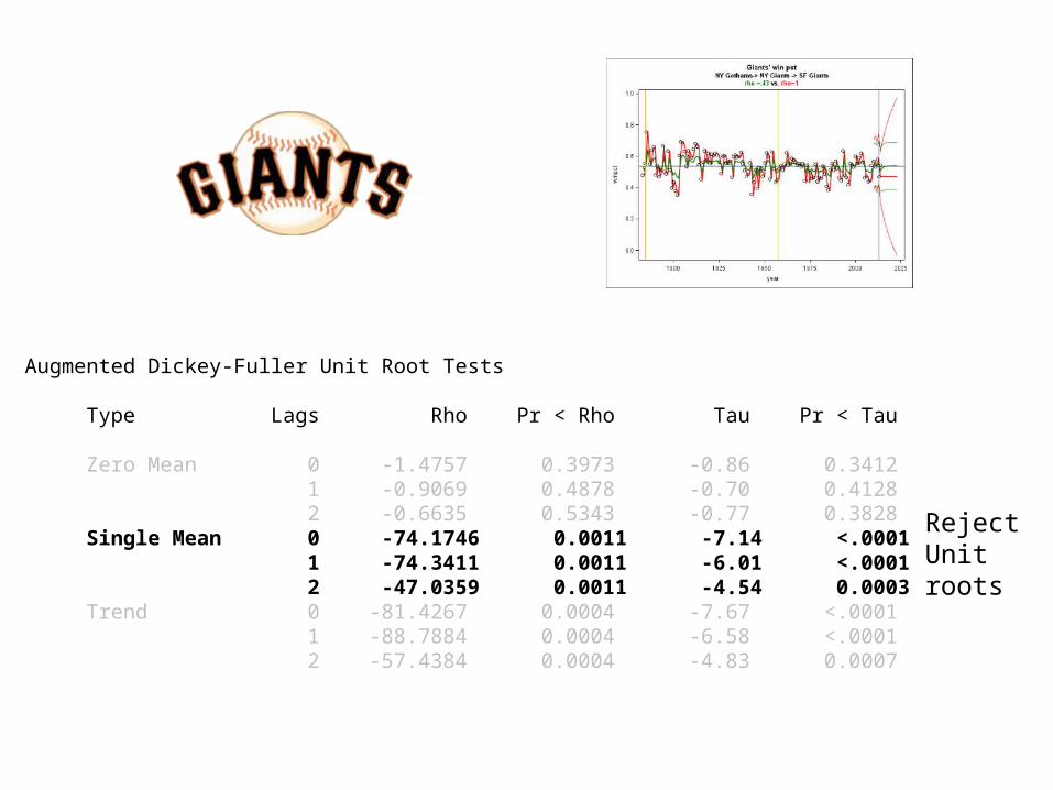
Augmented Dickey-Fuller Unit Root Tests

Type Lags Rho Pr < Rho Tau Pr < Tau

Zero Mean 0 -1.4757 0.3973 -0.86 0.3412 1 -0.9069 0.4878 -0.70 0.4128 2 -0.6635 0.5343 -0.77 0.3828 Single Mean 0 -74.1746 0.0011 -7.14 <.0001 1 -74.3411 0.0011 -6.01 <.0001 2 -47.0359 0.0011 -4.54 0.0003 Trend 0 -81.4267 0.0004 -7.67 <.0001 1 -88.7884 0.0004 -6.58 <.0001 2 -57.4384 0.0004 -4.83 0.0007

Reject Unit roots

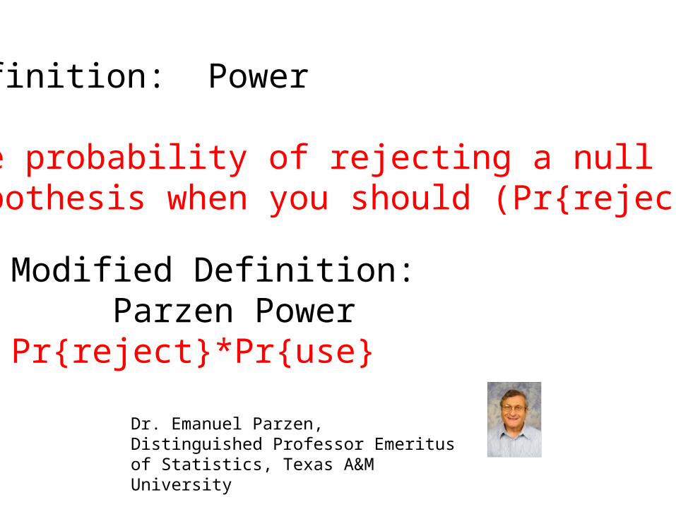
Modified Definition: Parzen PowerPr{reject}*Pr{use}

Definition: Power

The probability of rejecting a null hypothesis when you should (Pr{reject})

Dr. Emanuel Parzen, Distinguished Professor Emeritus of Statistics, Texas A&M University

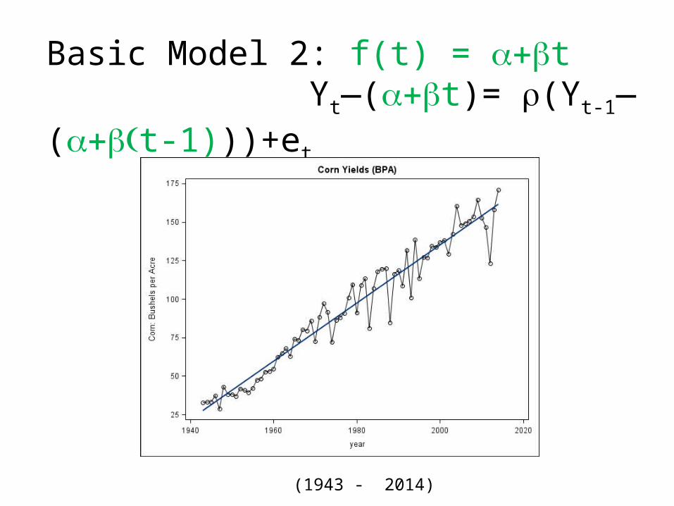
Basic Model 2: f(t) = +a bt Yt—( +a bt)= r(Yt-1—( + (a b t-1)))+et

(1943 - 2014)

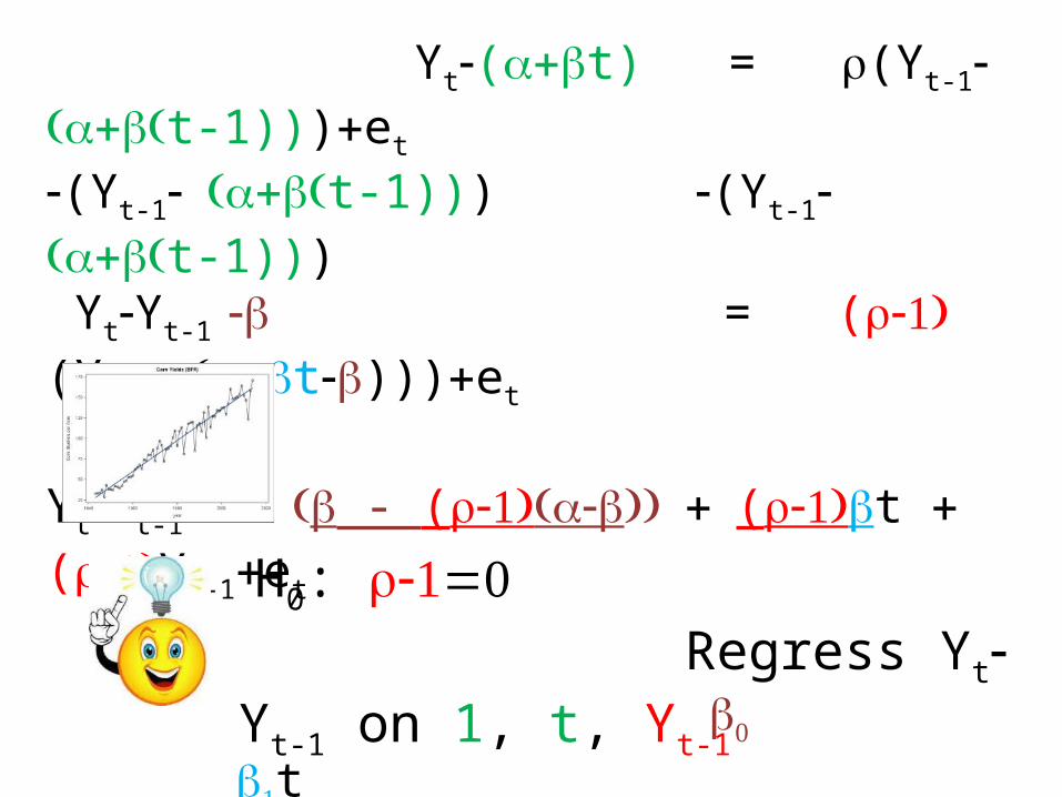
Yt-( +a bt) = r(Yt-1- ( + (a b t-1)))+et

-(Yt-1- ( + (a b t-1))) -(Yt-1- ( + (a b t-1))) Yt-Yt-1 -b = ( -1)r (Yt-1- (a+bt-b)))+et

Yt-Yt-1 = (b - ( -1)r ( -a b)) + ( -1)r bt + ( -1)r Yt-1+et

b0 b1t

H0: -1r =0 Regress Yt-Yt-1 on 1, t, Yt-1

t-stat

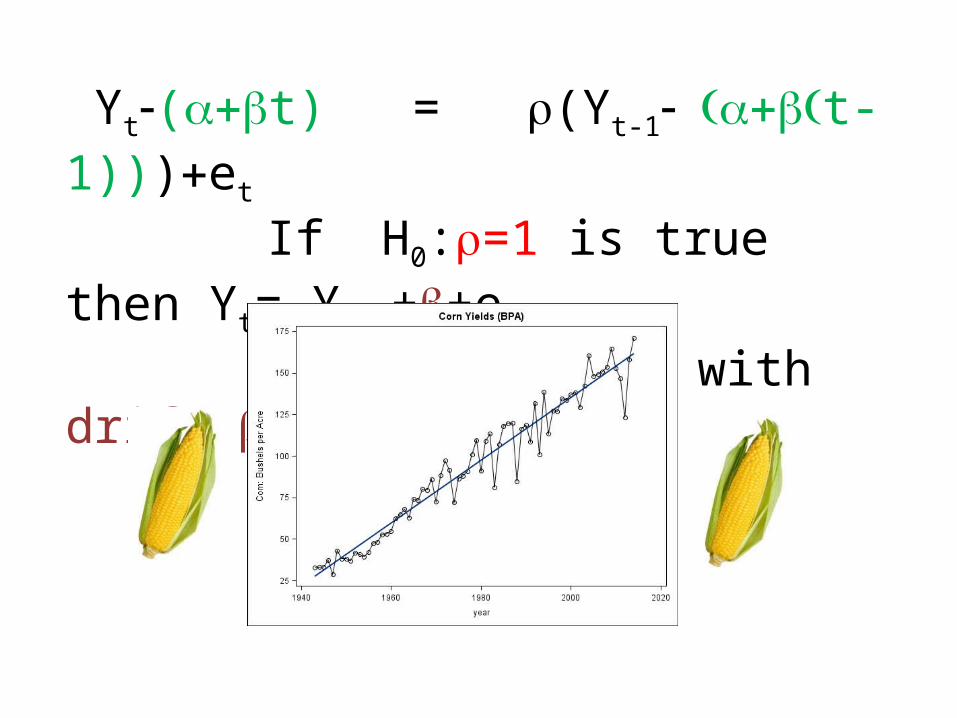
Yt-( +a bt) = r(Yt-1- ( + (a b t-1)))+et

If H0:r=1 is true then Yt= Yt-1+b+et random walk with drift b

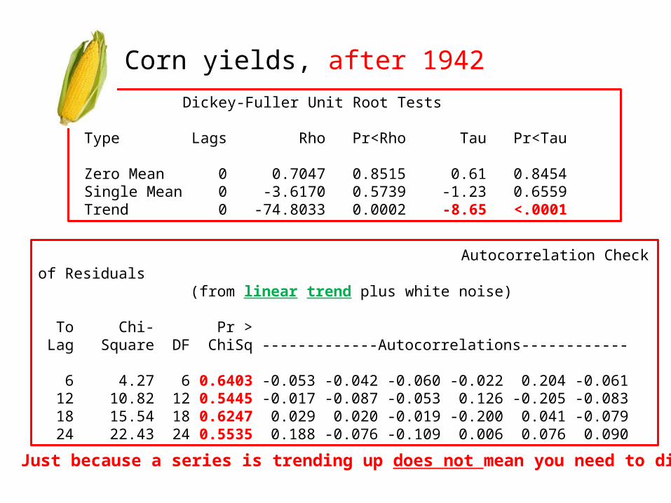
Corn yields, after 1942 Dickey-Fuller Unit Root Tests

Type Lags Rho Pr<Rho Tau Pr<Tau

Zero Mean 0 0.7047 0.8515 0.61 0.8454 Single Mean 0 -3.6170 0.5739 -1.23 0.6559 Trend 0 -74.8033 0.0002 -8.65 <.0001

Autocorrelation Check of Residuals (from linear trend plus white noise)

To Chi- Pr > Lag Square DF ChiSq -------------Autocorrelations------------

6 4.27 6 0.6403 -0.053 -0.042 -0.060 -0.022 0.204 -0.061 12 10.82 12 0.5445 -0.017 -0.087 -0.053 0.126 -0.205 -0.083 18 15.54 18 0.6247 0.029 0.020 -0.019 -0.200 0.041 -0.079 24 22.43 24 0.5535 0.188 -0.076 -0.109 0.006 0.076 0.090

Lesson 4: Just because a series is trending up does not mean you need to difference!

If we all worked on the assumption that what is accepted as true is really true, there would be little hope of advance. (Orville Wright)

Powered flight Kill Devil Hills NC, Dec. 1903

Lesson 4: Just because a series is trending up does not mean you need to difference!

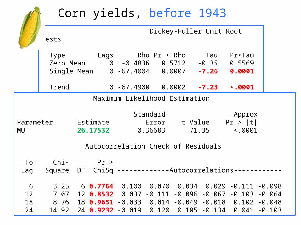
Corn yields, before 1943 Dickey-Fuller Unit Root Tests

Type Lags Rho Pr < Rho Tau Pr<Tau Zero Mean 0 -0.4836 0.5712 -0.35 0.5569 Single Mean 0 -67.4004 0.0007 -7.26 0.0001 Trend 0 -67.4900 0.0002 -7.23 <.0001

Maximum Likelihood Estimation

Standard ApproxParameter Estimate Error t Value Pr > |t| MU 26.17532 0.36683 71.35 <.0001

Autocorrelation Check of Residuals

To Chi- Pr > Lag Square DF ChiSq -------------Autocorrelations------------

6 3.25 6 0.7764 0.100 0.070 0.034 0.029 -0.111 -0.098 12 7.07 12 0.8532 0.037 -0.111 -0.096 -0.067 -0.103 -0.064 18 8.76 18 0.9651 -0.033 0.014 -0.049 -0.018 0.102 -0.048 24 14.92 24 0.9232 -0.019 0.120 0.105 -0.134 0.041 -0.103

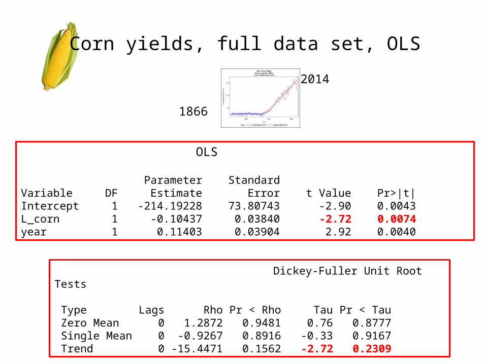
Corn yields, full data set, OLS

1866

2014

OLS

Parameter StandardVariable DF Estimate Error t Value Pr>|t|Intercept 1 -214.19228 73.80743 -2.90 0.0043L_corn 1 -0.10437 0.03840 -2.72 0.0074year 1 0.11403 0.03904 2.92 0.0040

Dickey-Fuller Unit Root Tests

Type Lags Rho Pr < Rho Tau Pr < Tau Zero Mean 0 1.2872 0.9481 0.76 0.8777 Single Mean 0 -0.9267 0.8916 -0.33 0.9167 Trend 0 -15.4471 0.1562 -2.72 0.2309

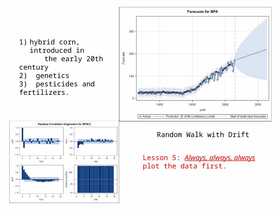
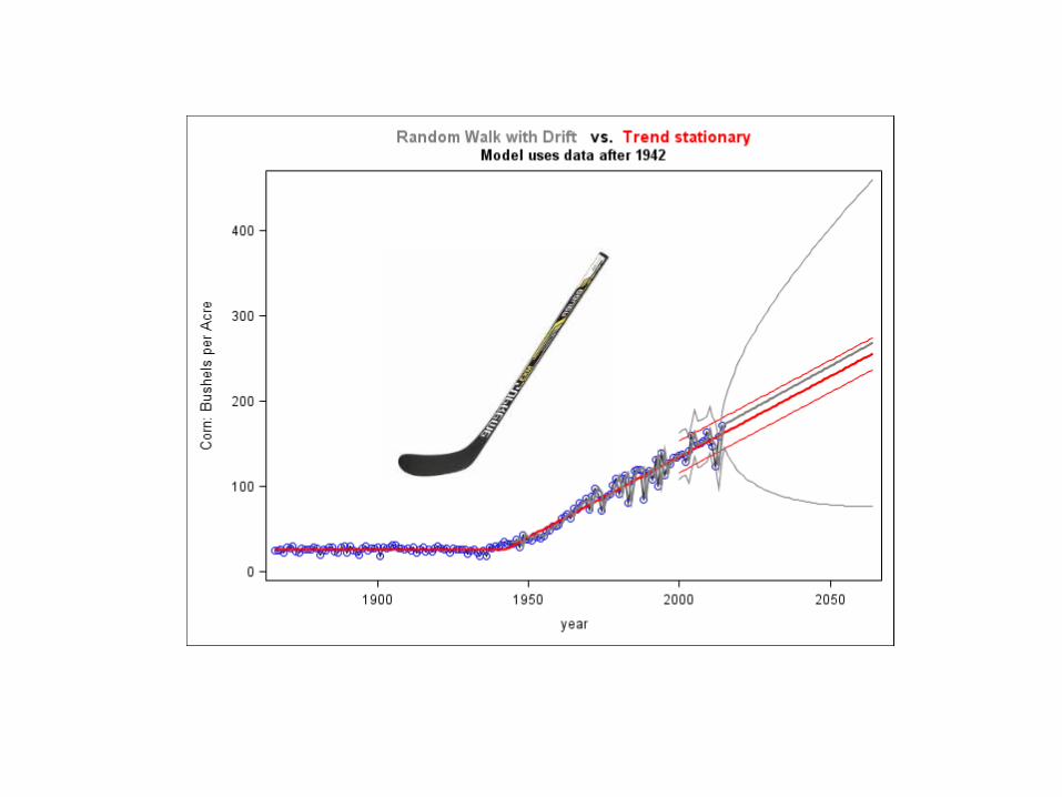
Random Walk with Drift

1) hybrid corn, introduced in the early 20th century 2) genetics3) pesticides and fertilizers.

Lesson 5: Always, always, always plot the data first.

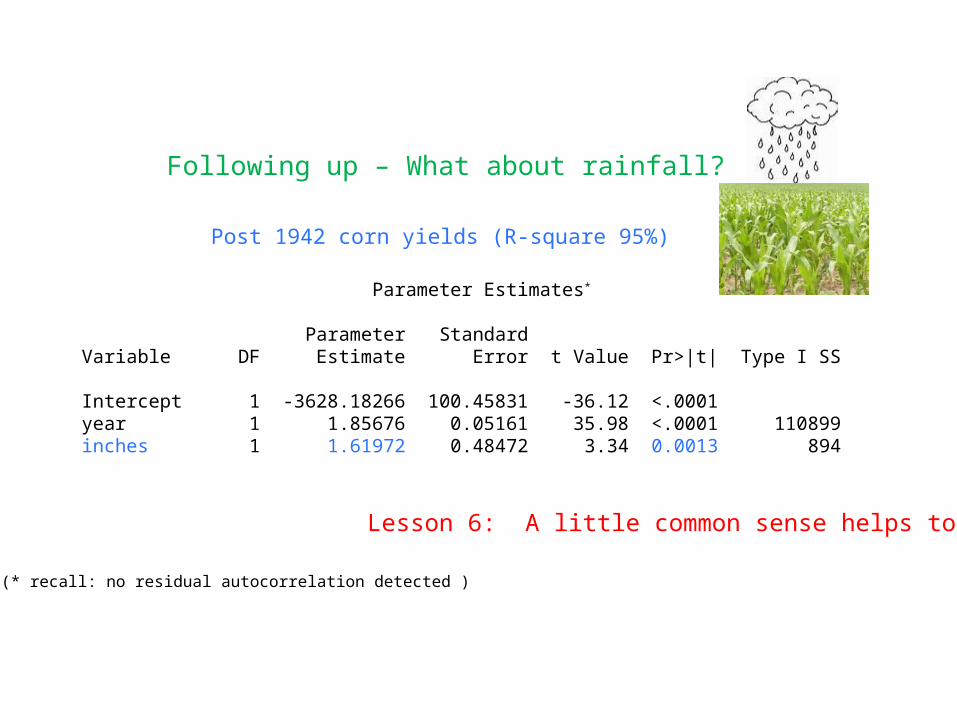
Following up – What about rainfall?

Post 1942 corn yields (R-square 95%)

Parameter Estimates*

Parameter StandardVariable DF Estimate Error t Value Pr>|t| Type I SS

Intercept 1 -3628.18266 100.45831 -36.12 <.0001 year 1 1.85676 0.05161 35.98 <.0001 110899inches 1 1.61972 0.48472 3.34 0.0013 894

(* recall: no residual autocorrelation detected )

Lesson 6: A little common sense helps too!

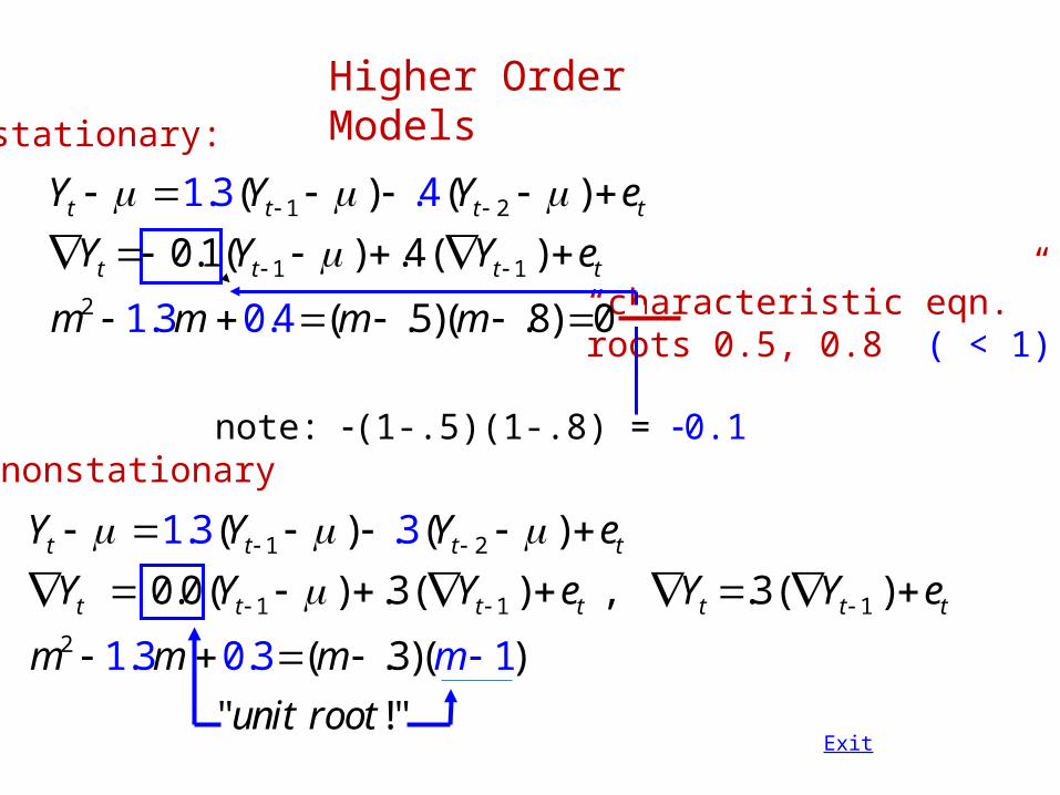
Higher Order Models

1 2

1 1

2

( ) ( )

0.1( ) .4( )

( .5)(

1.3 .4

1 .8). 0.4 03

t t t t

t t t t

Y Y Y e

Y Y Y e

m m m m

“characteristic eqn.”roots 0.5, 0.8 ( < 1)

1 2

1 1 1

2

( ) ( )

0.0( ) .3( ) , .3(

1.3 .3

1.3 0.3 1

)

( .3)( )

" !"

t t t t

t t t t t t t

Y Y Y e

Y Y Y e Y Y e

m m m

unit r t

m

oo

note: -(1-.5)(1-.8) = -0.1

stationary:

nonstationary

Exit

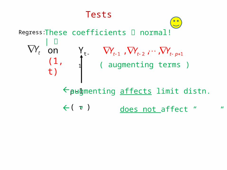
Tests

Regress:

tY 1 2 1, , ,t t t pY Y Y on (1, t) Yt-1

( augmenting terms )

r-1

( t )

augmenting affects limit distn.

“ does not affect “ “

These coefficients normal!| |

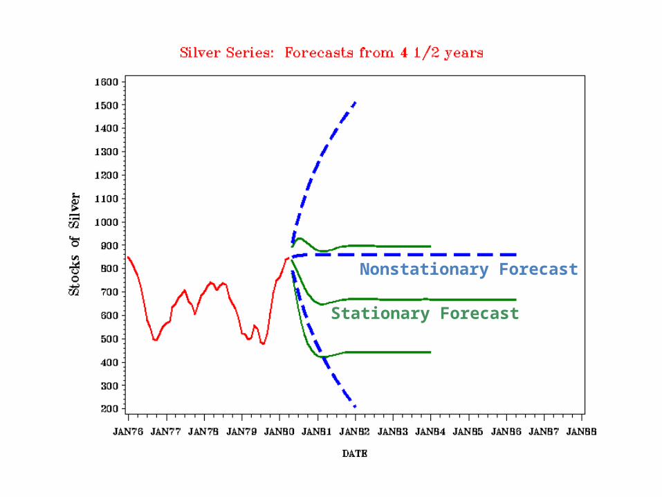
Nonstationary Forecast

Stationary Forecast

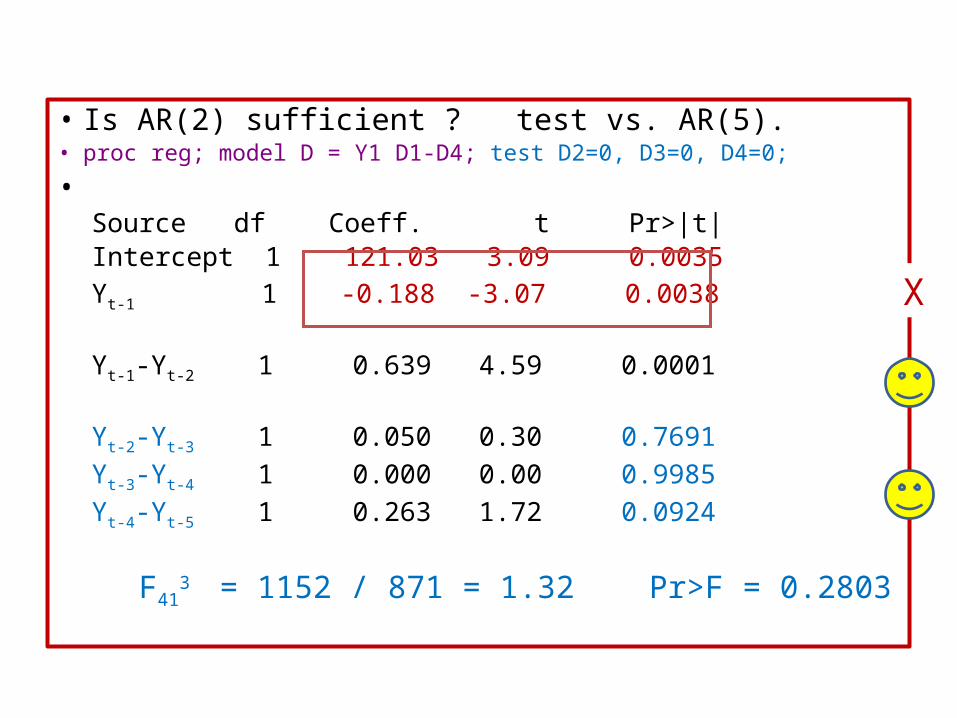
• Is AR(2) sufficient ? test vs. AR(5).• proc reg; model D = Y1 D1-D4; test D2=0, D3=0, D4=0;

• Source df Coeff. t Pr>|t|Intercept 1 121.03 3.09 0.0035Yt-1 1 -0.188 -3.07 0.0038

Yt-1-Yt-2 1 0.639 4.59 0.0001

Yt-2-Yt-3 1 0.050 0.30 0.7691Yt-3-Yt-4 1 0.000 0.00 0.9985Yt-4-Yt-5 1 0.263 1.72 0.0924

F413 = 1152 / 871 = 1.32 Pr>F = 0.2803

X

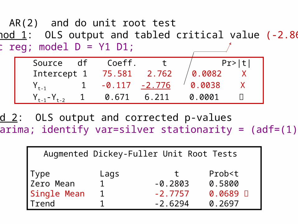
Fit AR(2) and do unit root testMethod 1: OLS output and tabled critical value (-2.86)proc reg; model D = Y1 D1;

Source df Coeff. t Pr>|t|Intercept 1 75.581 2.762 0.0082 XYt-1 1 -0.117 -2.776 0.0038 XYt-1-Yt-2 1 0.671 6.211 0.0001

Method 2: OLS output and corrected p-valuesproc arima; identify var=silver stationarity = (adf=(1));

Augmented Dickey-Fuller Unit Root Tests

Type Lags t Prob<t Zero Mean 1 -0.2803 0.5800 Single Mean 1 -2.7757 0.0689 Trend 1 -2.6294 0.2697

?

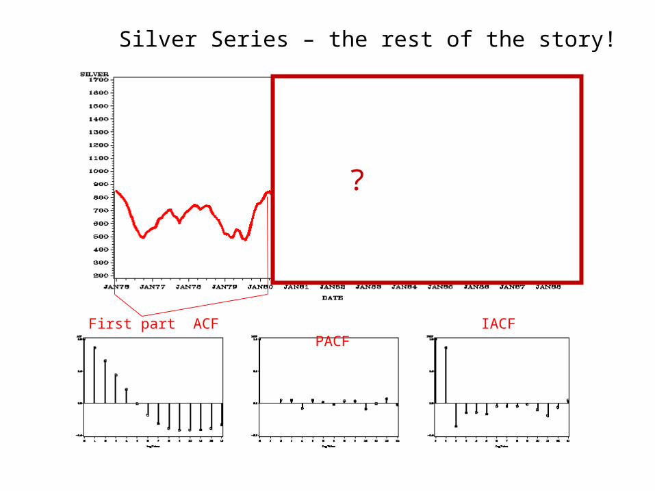
First part ACF IACF PACF

Silver Series – the rest of the story!

Your talk seems better now Grandpa!

Disclaimer: No babies ingested alcohol in the making of this slide. (I personally made sure the bottle was empty).

Exit

One Final Wilbur Wright Quote:

“If I were giving a young man advice as to how he might succeed in life, I would say to him, pick out a good father and mother, and begin life in Ohio.”

--Wilbur Wright, 1910

Wrights (& me) *

… and one from Clark Gable:

“I'm just a lucky slob from Ohio who happened to be in the right place at the right time.”

D. A. Dickey

=1r

The End

Lesson 8: Don’t take yourself too seriously