歐亞書局 P

19.5 Numeric Integration and DifferentiationApplications often lead to integrals whose analytic

evaluation would be very difficult or even impossible, or whose integrand is an empirical function given by recorded numeric values. Then we may obtain approximate numeric values of the integral by a numeric integration method.

continued817

歐亞書局 P

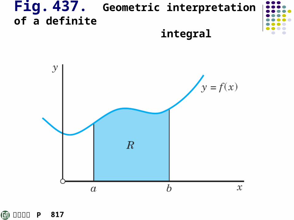
Fig. 437. Geometric interpretation of a definite integral

817

歐亞書局 P

Rectangular Rule. Trapezoidal Rule

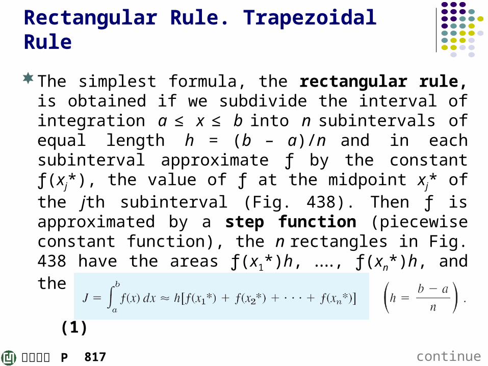
The simplest formula, the rectangular rule, is obtained if we subdivide the interval of integration a ≤ x ≤ b into n subintervals of equal length h = (b – a)/n and in each subinterval approximate ƒ by the constant ƒ(xj*), the value of ƒ at the midpoint xj* of the jth subinterval (Fig. 438). Then ƒ is approximated by a step function (piecewise constant function), the n rectangles in Fig. 438 have the areas ƒ(x1*)h, , ‥‥ƒ(xn*)h, and the rectangular rule is

(1)

continued817

歐亞書局 P

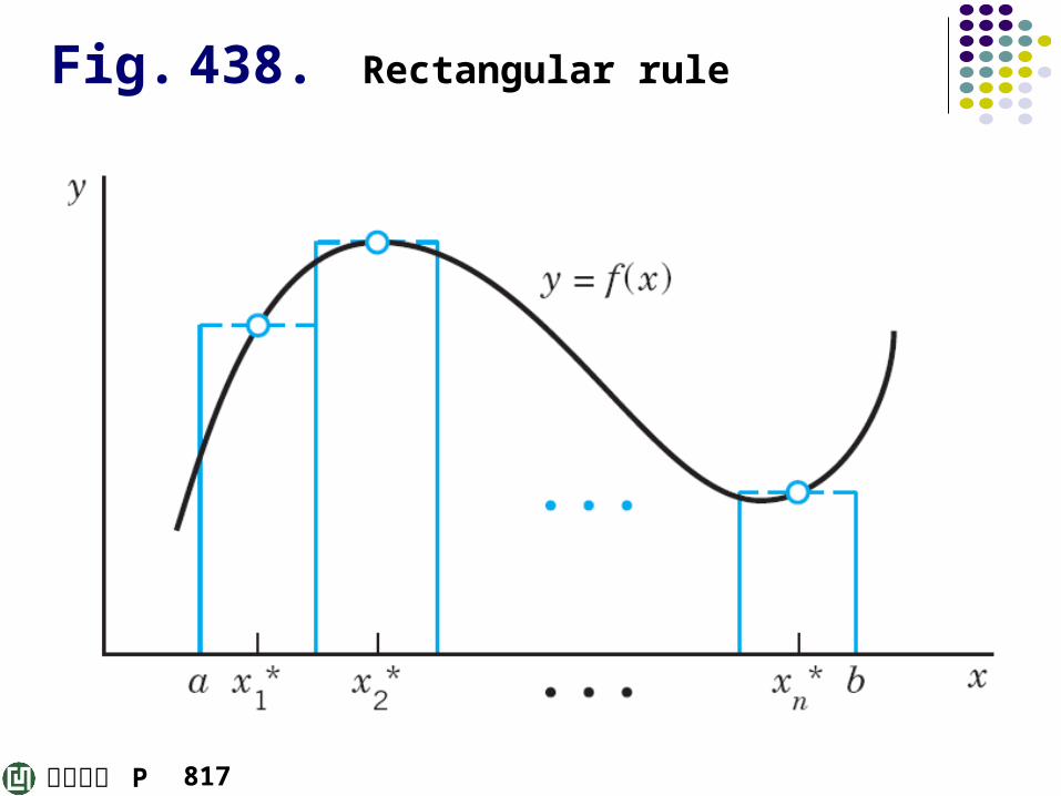
Fig. 438. Rectangular rule

817

歐亞書局 P

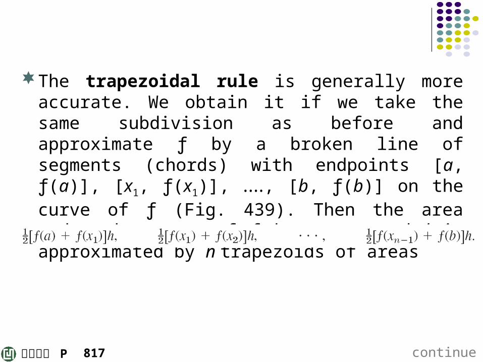
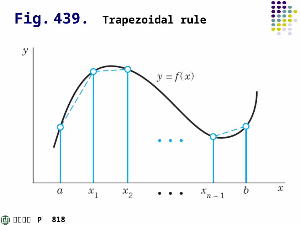
The trapezoidal rule is generally more accurate. We obtain it if we take the same subdivision as before and approximate ƒ by a broken line of segments (chords) with endpoints [a, ƒ(a)], [x1, ƒ(x1)], , [‥‥ b, ƒ(b)] on the curve of ƒ (Fig. 439). Then the area under the curve of ƒ between a and b is approximated by n trapezoids of areas

continued817

歐亞書局 P

Fig. 439. Trapezoidal rule

818

歐亞書局 P

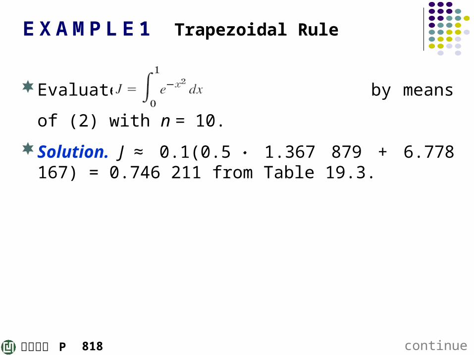
E X A M P L E 1 Trapezoidal Rule

Evaluate by means of (2) with n = 10.

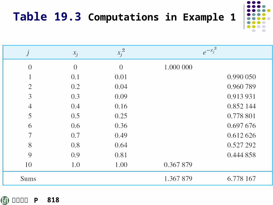
Solution. J ≈ 0.1(0.5 ۰ 1.367 879 + 6.778 167) = 0.746 211 from Table 19.3.

continued818

歐亞書局 P

Table 19.3 Computations in Example 1

818

歐亞書局 P

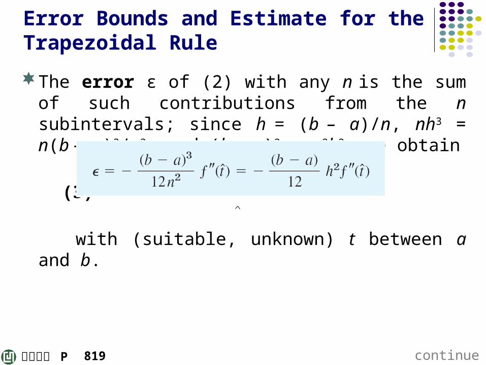
Error Bounds and Estimate for the Trapezoidal Rule

The error ε of (2) with any n is the sum of such contributions from the n subintervals; since h = (b – a)/n, nh3 = n(b – a)3/n3, and (b – a)2 = n2h2, we obtain

(3)

with (suitable, unknown) t between a and b.

continued819

歐亞書局 P

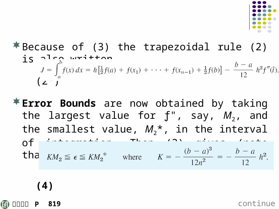
Because of (3) the trapezoidal rule (2) is also written

(2*)

Error Bounds are now obtained by taking the largest value for ƒ", say, M2, and the smallest value, M2*, in the interval of integration. Then (3) gives (note that K is negative)

(4)

continued819

歐亞書局 P

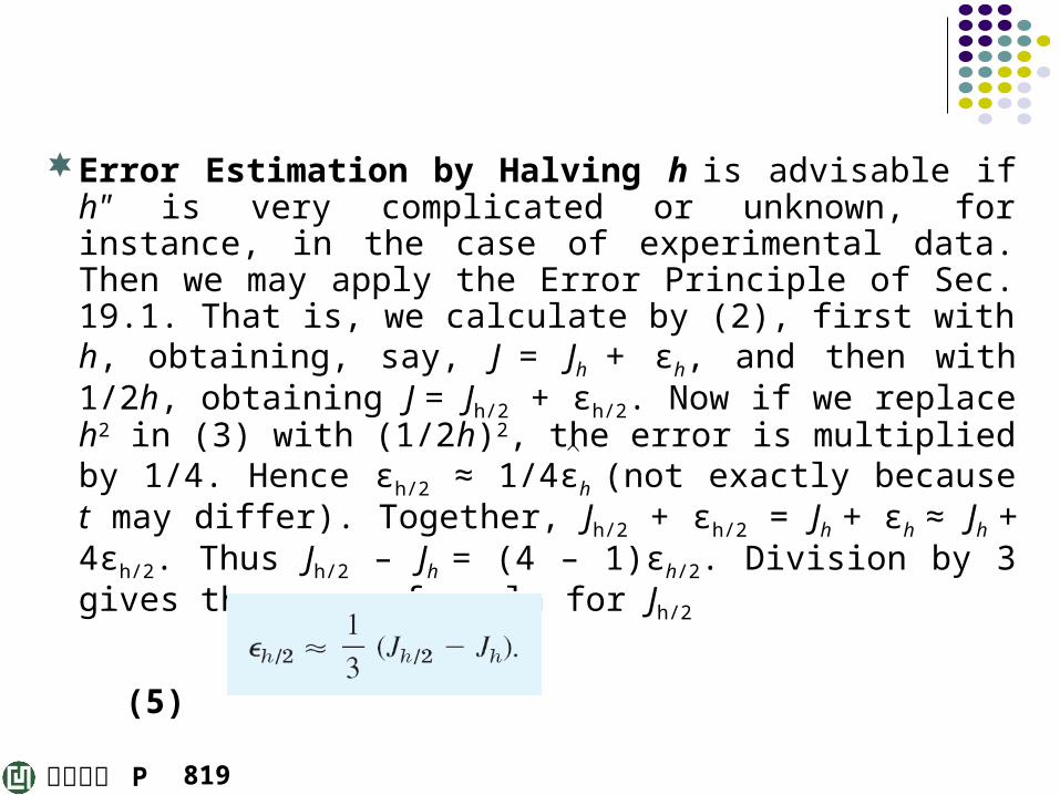
Error Estimation by Halving h is advisable if h" is very complicated or unknown, for instance, in the case of experimental data. Then we may apply the Error Principle of Sec. 19.1. That is, we calculate by (2), first with h, obtaining, say, J = Jh + εh, and then with 1/2h, obtaining J = Jh/2 + εh/2. Now if we replace h2 in (3) with (1/2h)2, the error is multiplied by 1/4. Hence εh/2 ≈ 1/4εh (not exactly because t may differ). Together, Jh/2 + εh/2 = Jh + εh ≈ Jh + 4εh/2. Thus Jh/2 – Jh = (4 – 1)εh/2. Division by 3 gives the error formula for Jh/2

(5)

819

歐亞書局 P

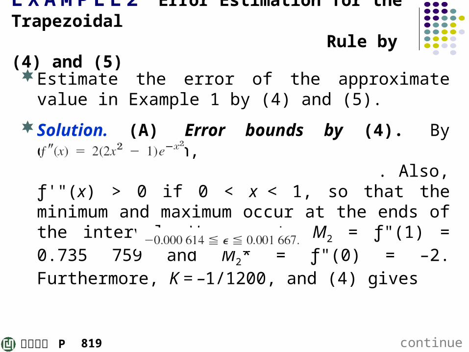
E X A M P L E 2 Error Estimation for the Trapezoidal Rule by (4) and (5)

Estimate the error of the approximate value in Example 1 by (4) and (5).

Solution. (A) Error bounds by (4). By differentiation, . Also, ƒ'"(x) > 0 if 0 < x < 1, so that the minimum and maximum occur at the ends of the interval. We compute M2 = ƒ"(1) = 0.735 759 and M2* = ƒ"(0) = –2. Furthermore, K = –1/1200, and (4) gives

continued819

歐亞書局 P

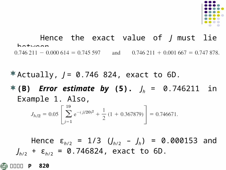
Hence the exact value of J must lie between

Actually, J = 0.746 824, exact to 6D.

(B) Error estimate by (5). Jh = 0.746211 in Example 1. Also,

Hence εh/2 = 1/3 (Jh/2 – Jh) = 0.000153 and Jh/2 + εh/2 = 0.746824, exact to 6D.

820

歐亞書局 P

Simpson’s Rule of Integration

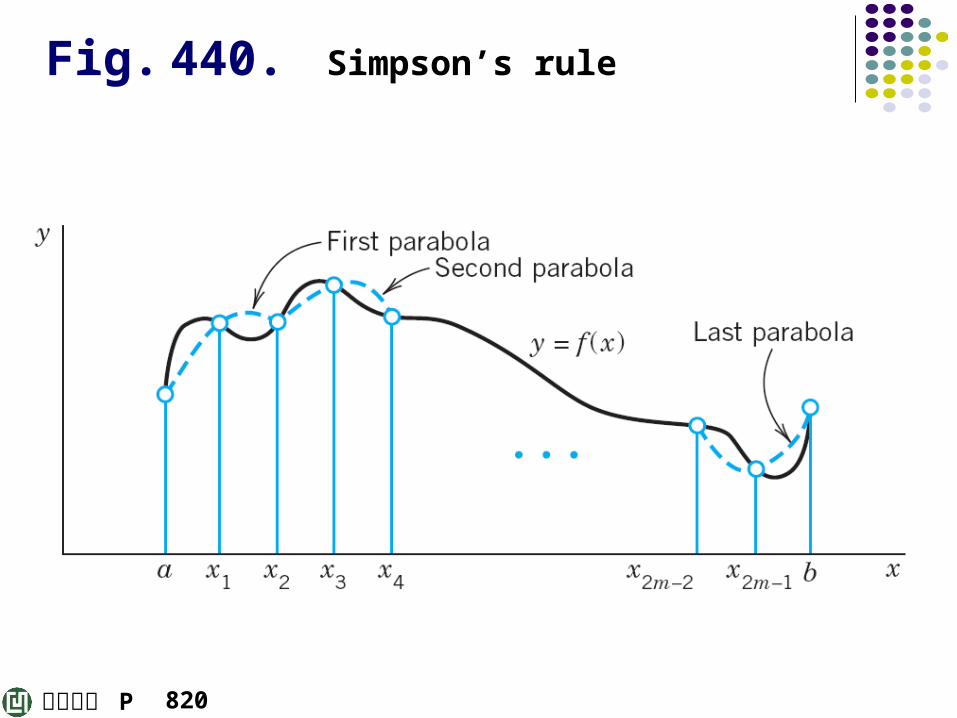
To derive Simpson’s rule, we divide the interval of integration a ≤ x ≤ b into an even number of equal subintervals, say, into n = 2m subintervals of length h = (b – a)/(2m), with endpoints x0 (= a), x1, , ‥‥ x2m-1, x2m (= b); see Fig. 440. We now take the first two subintervals and approximate ƒ(x) in the interval x0 ≤ x ≤ x2 = x0 + 2h by the Lagrange polynomial p2(x) through (x0, ƒ0), (x1, ƒ1), (x2, ƒ2), where ƒj = ƒ(xj).

continued820

歐亞書局 P

Fig. 440. Simpson’s rule

820

歐亞書局 P

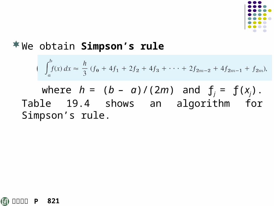
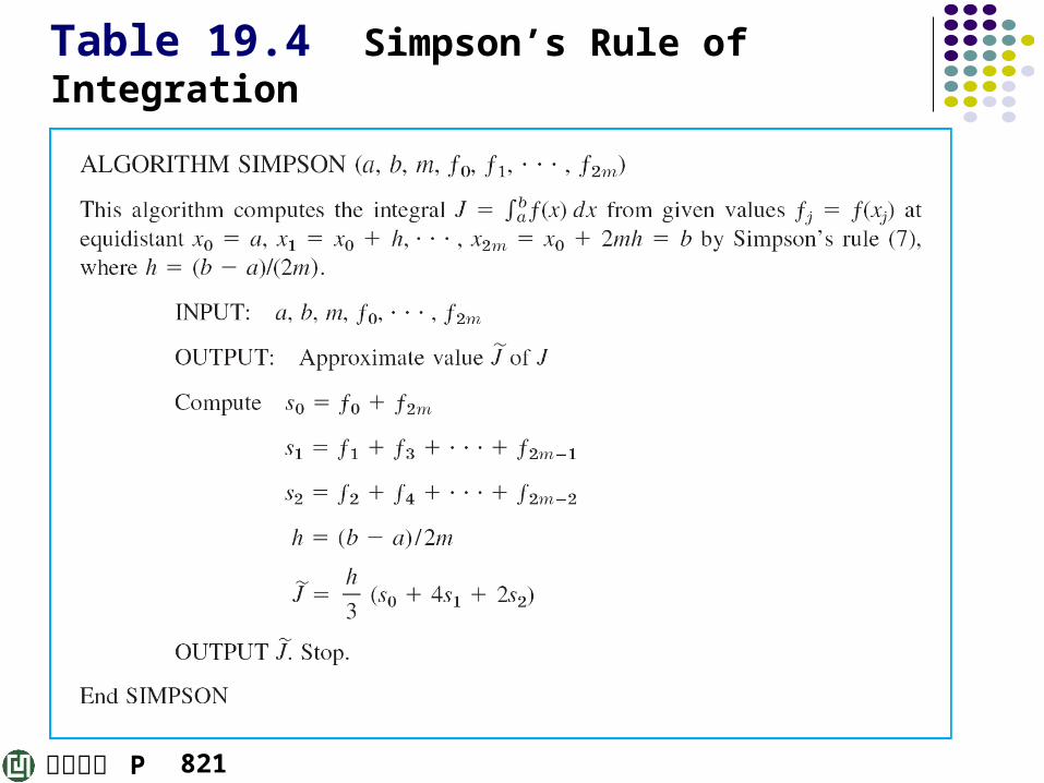
We obtain Simpson’s rule

(7)

where h = (b – a)/(2m) and ƒj = ƒ(xj). Table 19.4 shows an algorithm for Simpson’s rule.

821

歐亞書局 P

Table 19.4 Simpson’s Rule of Integration

821

歐亞書局 P

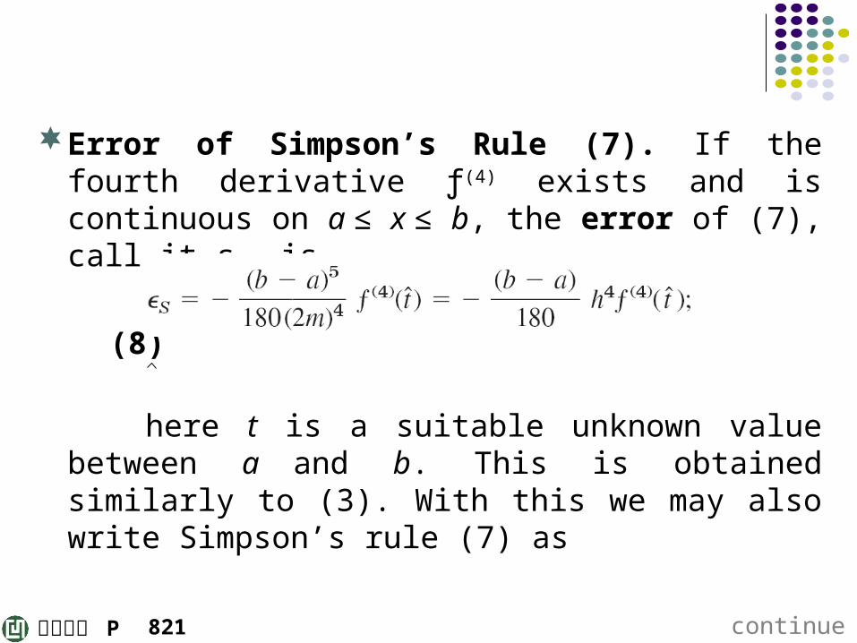
Error of Simpson’s Rule (7). If the fourth derivative ƒ(4) exists and is continuous on a ≤ x ≤ b, the error of (7), call it εS, is

(8)

here t is a suitable unknown value between a and b. This is obtained similarly to (3). With this we may also write Simpson’s rule (7) as

continued821

歐亞書局 P

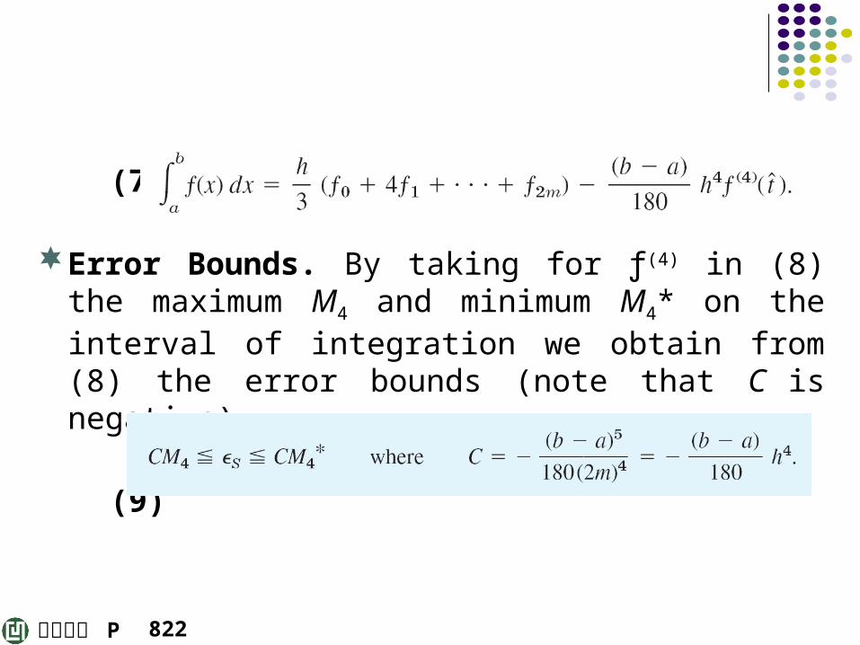
(7**)

Error Bounds. By taking for ƒ(4) in (8) the maximum M4 and minimum M4* on the interval of integration we obtain from (8) the error bounds (note that C is negative)

(9)

822

歐亞書局 P

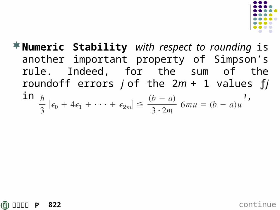
Numeric Stability with respect to rounding is another important property of Simpson’s rule. Indeed, for the sum of the roundoff errors j of the 2m + 1 values ƒj in (7) we obtain, since h = (b – a)/2m,

continued822

歐亞書局 P

where u is the rounding unit (u = 1/2 ۰ 10-6 if we round off to 6D; see Sec. 19.1). Also 6 = 1 + 4 + 1 is the sum of the coefficients for a pair of intervals in (7); take m = 1 in (7) to see this. The bound (b – a)u is independent of m, so that it cannot increase with increasing m, that is, with decreasing h. This proves stability.

822

歐亞書局 P

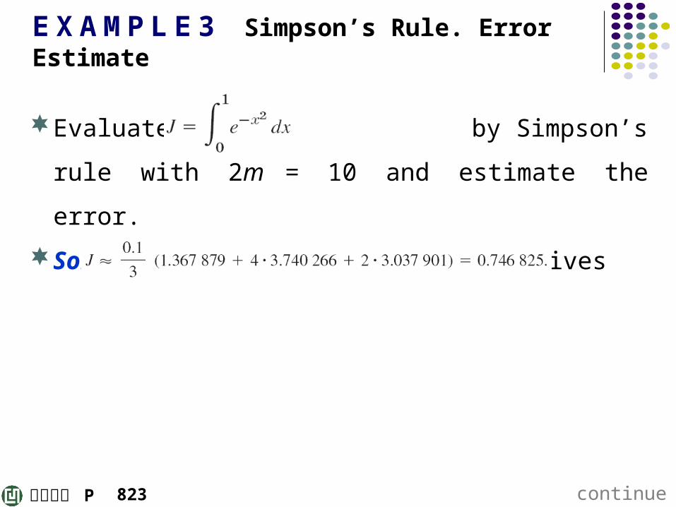
E X A M P L E 3 Simpson’s Rule. Error Estimate

Evaluate by Simpson’s rule with 2m = 10

and estimate the error.

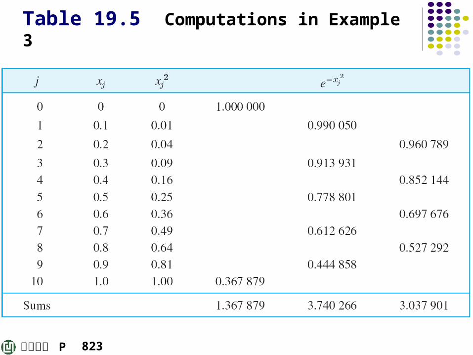
Solution. Since h = 0.1, Table 19.5 gives

continued823

歐亞書局 P

Estimate of error. Differentiation gives . By considering the derivative ƒ(5) of ƒ(4) we

find that the largest value of ƒ(4) in the interval of integration occurs at 0 and the smallest value at

. Computation gives the values M4 = ƒ(4)

(0) = 12 and M4* = ƒ(4)(x*) = –7.419. Since 2m = 10 and b – a = 1, we obtain C = –1/1 800 000 = –0.000 000 56. Therefore, from (9),

continued823

歐亞書局 P

Hence J must lie between 0.746 825 – 0.000 007 = 0.746 818 and 0.746 825 + 0.000 005 = 0.746 830, so that at least four digits of our approximate value are exact. Actually, the value 0.746 825 is exact to 5D because J = 0.746 824 (exact to 6D).

Thus our result is much better than that in Example 1 obtained by the trapezoidal rule, whereas the number of operations is nearly the same in both cases.

continued823

歐亞書局 P

Table 19.5 Computations in Example 3

823

歐亞書局 P

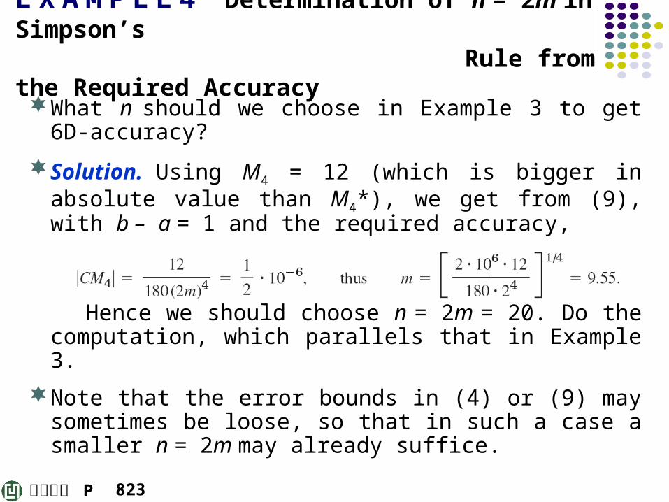
E X A M P L E 4 Determination of n = 2m in Simpson’s Rule from the Required Accuracy

What n should we choose in Example 3 to get 6D-accuracy?

Solution. Using M4 = 12 (which is bigger in absolute value than M4*), we get from (9), with b – a = 1 and the required accuracy,

Hence we should choose n = 2m = 20. Do the computation, which parallels that in Example 3.

Note that the error bounds in (4) or (9) may sometimes be loose, so that in such a case a smaller n = 2m may already suffice.

823

歐亞書局 P

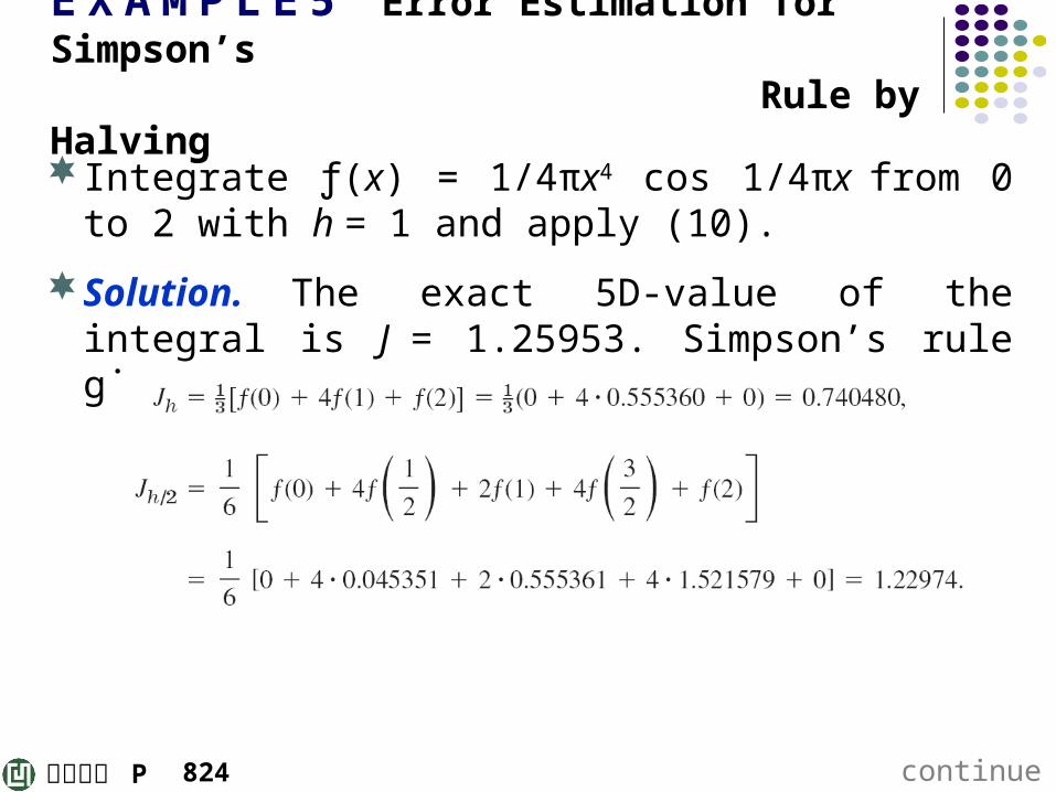
E X A M P L E 5 Error Estimation for Simpson’s Rule by Halving

Integrate ƒ(x) = 1/4πx4 cos 1/4πx from 0 to 2 with h = 1 and apply (10).

Solution. The exact 5D-value of the integral is J = 1.25953. Simpson’s rule gives

continued824

歐亞書局 P

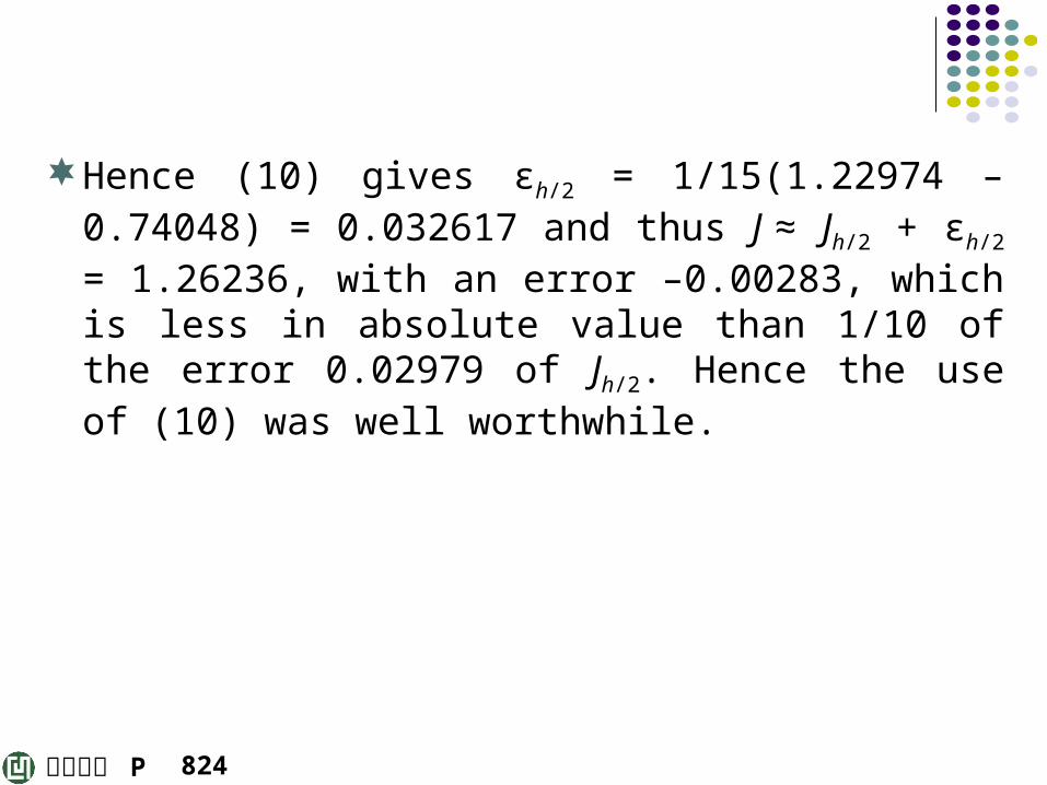
Hence (10) gives εh/2 = 1/15(1.22974 – 0.74048) = 0.032617 and thus J ≈ Jh/2 + εh/2 = 1.26236, with an error –0.00283, which is less in absolute value than 1/10 of the error 0.02979 of Jh/2. Hence the use of (10) was well worthwhile.

824

歐亞書局 P

Adaptive Integration

The idea is to adapt step h to the variability of ƒ(x). That is, where ƒ varies but little, we can proceed in large steps without causing a substantial error in the integral, but where ƒ varies rapidly, we have to take small steps in order to stay everywhere close enough to the curve of ƒ.

824

歐亞書局 P

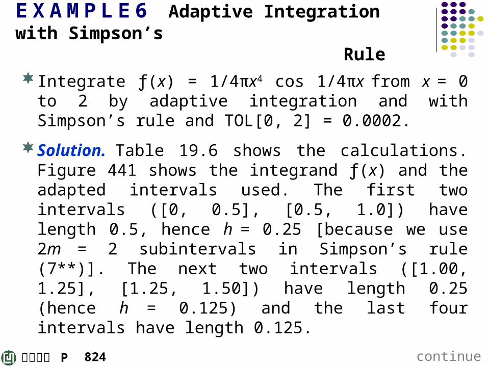
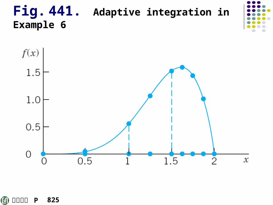
E X A M P L E 6 Adaptive Integration with Simpson’s Rule

Integrate ƒ(x) = 1/4πx4 cos 1/4πx from x = 0 to 2 by adaptive integration and with Simpson’s rule and TOL[0, 2] = 0.0002.

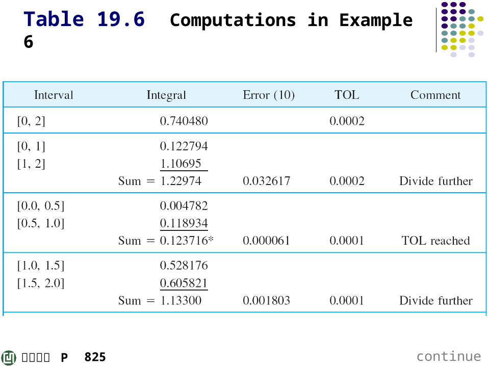
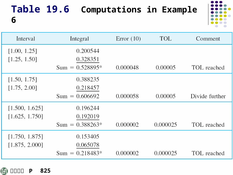
Solution. Table 19.6 shows the calculations. Figure 441 shows the integrand ƒ(x) and the adapted intervals used. The first two intervals ([0, 0.5], [0.5, 1.0]) have length 0.5, hence h = 0.25 [because we use 2m = 2 subintervals in Simpson’s rule (7**)]. The next two intervals ([1.00, 1.25], [1.25, 1.50]) have length 0.25 (hence h = 0.125) and the last four intervals have length 0.125.

continued824

歐亞書局 P

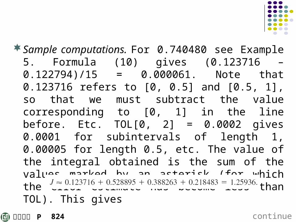
Sample computations. For 0.740480 see Example 5. Formula (10) gives (0.123716 – 0.122794)/15 = 0.000061. Note that 0.123716 refers to [0, 0.5] and [0.5, 1], so that we must subtract the value corresponding to [0, 1] in the line before. Etc. TOL[0, 2] = 0.0002 gives 0.0001 for subintervals of length 1, 0.00005 for length 0.5, etc. The value of the integral obtained is the sum of the values marked by an asterisk (for which the error estimate has become less than TOL). This gives

continued824

歐亞書局 P

The exact 5D-value is J = 1.25953. Hence the error is 0.00017. This is about 1/200 of the absolute value of that in Example 5. Our more extensive computation has produced a much better result.

continued825

歐亞書局 P

Table 19.6 Computations in Example 6

continued825

歐亞書局 P

Table 19.6 Computations in Example 6

825

歐亞書局 P

Fig. 441. Adaptive integration in Example 6

825

歐亞書局 P

Gauss Integration FormulasMaximum Degree of Precision

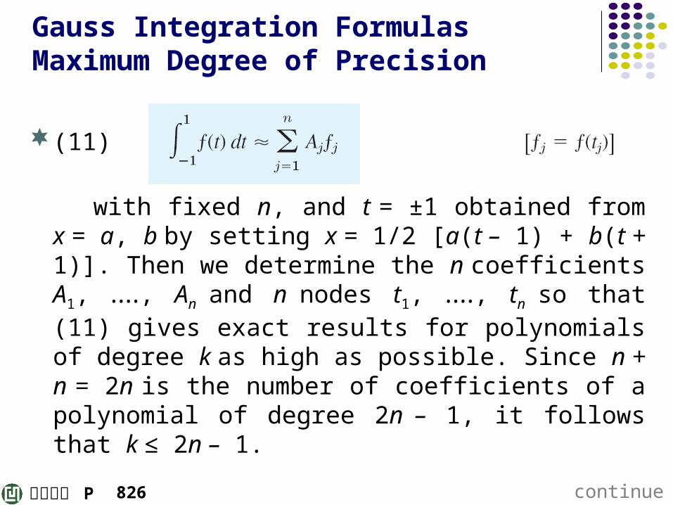
(11)

with fixed n, and t = ±1 obtained from x = a, b by setting x = 1/2 [a(t – 1) + b(t + 1)]. Then we determine the n coefficients A1, , ‥‥ An and n nodes t1, , ‥‥ tn so that (11) gives exact results for polynomials of degree k as high as possible. Since n + n = 2n is the number of coefficients of a polynomial of degree 2n – 1, it follows that k ≤ 2n – 1.

continued826

歐亞書局 P

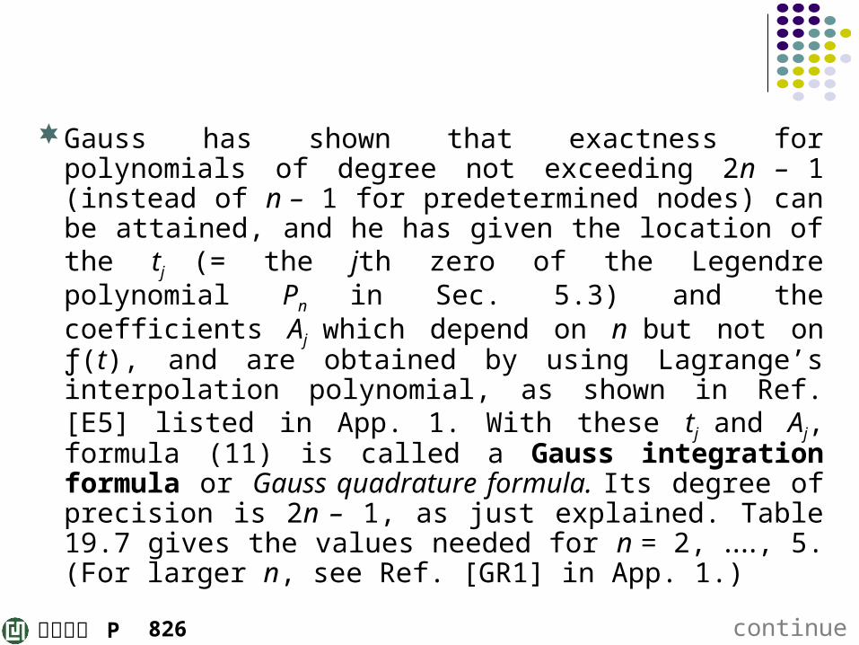
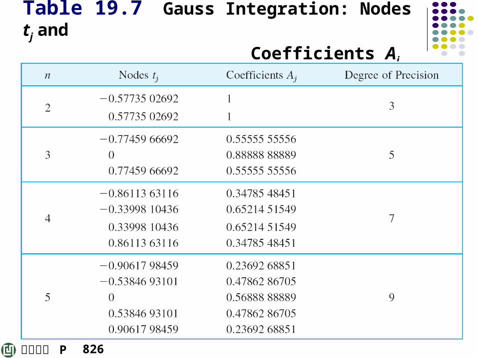
Gauss has shown that exactness for polynomials of degree not exceeding 2n – 1 (instead of n – 1 for predetermined nodes) can be attained, and he has given the location of the tj (= the jth zero of the Legendre polynomial Pn in Sec. 5.3) and the coefficients Aj which depend on n but not on ƒ(t), and are obtained by using Lagrange’s interpolation polynomial, as shown in Ref. [E5] listed in App. 1. With these tj and Aj, formula (11) is called a Gauss integration formula or Gauss quadrature formula. Its degree of precision is 2n – 1, as just explained. Table 19.7 gives the values needed for n = 2, , 5. (For ‥‥larger n, see Ref. [GR1] in App. 1.)

continued826

歐亞書局 P

Table 19.7 Gauss Integration: Nodes tj and Coefficients Aj

826

歐亞書局 P

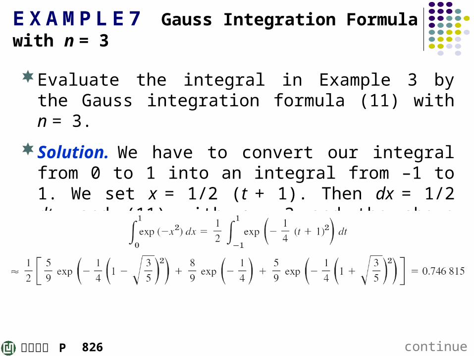
E X A M P L E 7 Gauss Integration Formula with n = 3

Evaluate the integral in Example 3 by the Gauss integration formula (11) with n = 3.

Solution. We have to convert our integral from 0 to 1 into an integral from –1 to 1. We set x = 1/2 (t + 1). Then dx = 1/2 dt, and (11) with n = 3 and the above values of the nodes and the coefficients yields

continued826

歐亞書局 P

(exact to 6D: 0.746 825), which is almost as accurate as the Simpson result obtained in Example 3 with a much larger number of arithmetic operations. With 3 function values (as in this example) and Simpson’s rule we would get 1/6 (1 + 4e-0.25 + e-1) = 0.747 180, with an error over 30 times that of the Gauss integration.

827

歐亞書局 P

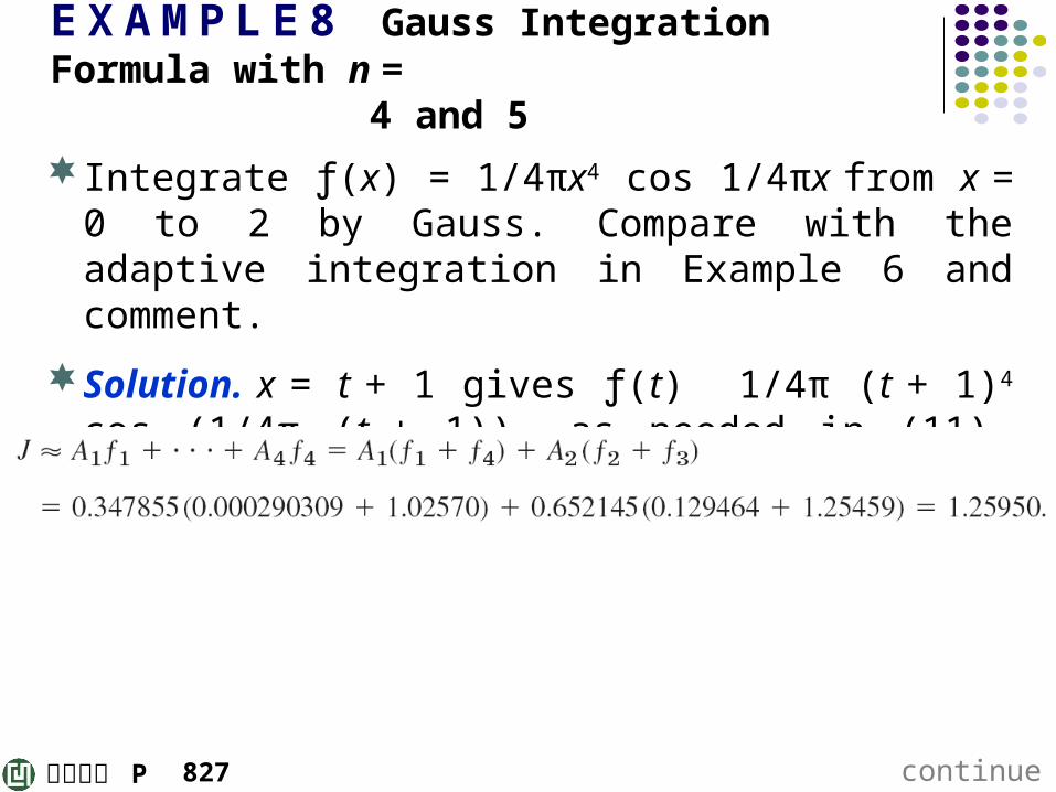
E X A M P L E 8 Gauss Integration Formula with n = 4 and 5

Integrate ƒ(x) = 1/4πx4 cos 1/4πx from x = 0 to 2 by Gauss. Compare with the adaptive integration in Example 6 and comment.

Solution. x = t + 1 gives ƒ(t) 1/4π (t + 1)4 cos (1/4π (t + 1)), as needed in (11). For n = 4 we calculate (6S)

continued827

歐亞書局 P

The error is 0.00003 because J = 1.25953 (6S). Calculating with 10S and n = 4 gives the same result; so the error is due to the formula, not rounding. For n = 5 and 10S we get J ≈ 1.25952 6185, too large by the amount 0.00000 0250 because J = 1.25952 5935 (10S). The accuracy is impressive, particularly if we compare the amount of work with that in Example 6.

827