Embed Size (px)
Citation preview
1
Civil Systems PlanningBenefit/Cost Analysis
Scott Matthews/Joe MarriottFinal ReviewCourses: 12-706 and 73-359Lecture 22 - 12/1/2004

Lecture 21: 11/28/01 12-706 and 73-359 2
Admin
PS 4 Returned TodayPS 5 Due Dec 10 (at final: last
chance)

Lecture 21: 11/28/01 12-706 and 73-359 3
Test Notes
Is cumulative, but “end-weighted”About 4 questions (2 decided already)
‘One’ may be a series of short questions Some HW questions were ‘previous year final
questions’E.g. CARB, DGPS, cash flows
Open book, notes, lecture notes Can Bring calculators (no laptops - shouldn’t
need them - I will provide P|F,i,n values)All slides in this talk from earlier classes

Lecture 21: 11/28/01 12-706 and 73-359 4
Test Hints
I will not try to ‘trick’ youWill be designed for 100 mins, but will have
3 hours to finish - don’t feel need to use whole time! Please!
Do not re-read text - skim familiar areas, ensure knowledge of others
Re-familiarize yourself with handouts And ‘energy problems’
Look for ‘shortcuts’ (e.g. relative NPV)

Lecture 21: 11/28/01 12-706 and 73-359 5
Three Legs to Stand On
Pareto Efficiency Make some better / make none worse
Kaldor-Hicks Program adopted (NB>0) if winners
COULD compensate losers, still be betterFundamental Principle of CBA
Amongst choices, select option with highest net benefit

Lecture 21: 11/28/01 12-706 and 73-359 6
$100
$1000
The ‘pareto frontier’ is the set of allocations that are pareto efficent. Try improving on (25,75) or (50,50) or (75,25)…We said initial alloc. mattered - e.g. (100,0)?
$25
$25

Lecture 21: 11/28/01 12-706 and 73-359 7
Gross Benefits with WTPPrice
Quantity
P*
0 1 2 3 4 Q*
A
BA
B
Total/Gross Benefits = area under curve = A+B = willingness to pay for all people = Social WTP = their benefit from consuming

Lecture 21: 11/28/01 12-706 and 73-359 8
Consumer Surplus Changes Price
Quantity
P*
0 1 2 Q* Q1
A
BP1
CS2
CS2 is the new consumer surplus when price decreases to (P1, Q1)
Change in CS = Trapezoid P*ABP1 = gain = positive net benefits

Lecture 21: 11/28/01 12-706 and 73-359 9
Elasticities of Demand
Measurement of how “responsive” demand is to some change in price or income.
Slope of demand curve = p/q.Elasticity of demand, , is defined to
be the percent change in quantity divided by the percent change in price. = p q / q p
Lecture 21: 11/28/01 12-706 and 73-359 10
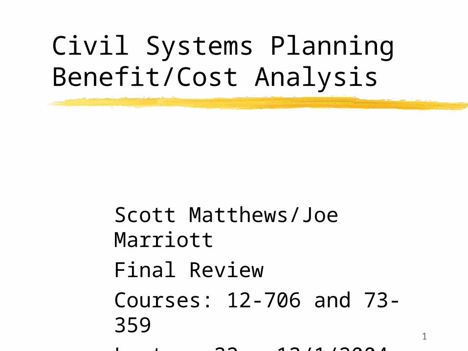
Social Surplus
Social Surplus = consumer surplus + producer surplusLosses in Social Surplus are Dead-Weight Losses!
Q
P
Q*
P*
S
D

Lecture 21: 11/28/01 12-706 and 73-359 11
General Terms
FV = $X (1+i)n
X : present value, i:interest rate and n is number of periods (eg years) of interest
Rule of 72PV = $X / (1+i)n
NPV=NPV(B) - NPV(C) (over time)Real vs. Nominal values

Lecture 21: 11/28/01 12-706 and 73-359 12
Notes on Estimation
Move from abstract to concrete, identifying assumptions
Draw from experience and basic data sources
Use statistical techniques/surveys if neededBe creative, BUTBe logical and able to justifyFind answer, then learn from it.Apply a reasonableness test

Lecture 21: 11/28/01 12-706 and 73-359 13
Equivalent Annual Benefit
EANB=NPV/Annuity Factor Annuity factor (i=5%,n=70) = 19.343 Ann. Factor (i=5%,n=35) = 16.374
EANB(1)=$25.73/19.343=$1.330EANB(2)=$18.77/16.374=$1.146
Still higher for option 1Note we assumed end of period pays

Lecture 21: 11/28/01 12-706 and 73-359 14
Internal Rate of Return
Defined as the discount rate where NPV=0
Graphically it is between 8-9%But we could solve otherwise
E.g. 0=-100k/(1+i) + 150k /(1+i)2 100k/(1+i) = 150k /(1+i)2
100k = 150k /(1+i) <=> 1+i = 1.5, i=50% -100k/1.5 + 150k /(1.5)2 <=> -66.67+66.67

Lecture 21: 11/28/01 12-706 and 73-359 15
Relative NPV Analysis
If comparing, can just find ‘relative’ NPV compared to a single option E.g. homework 2 copier problem Solutions NPV(1)=-$18k , NPV(2)=-$16k
Net difference between them was $1,536
Alternatively consider ‘net amounts’ Copier cost =-3k, salvage 2k, annual +1k -3k+(2k/1.14)+(+1k/1.1)+..+(+1k/1.14) -3k+(2k*.683) +3.1699k = $1,536

Lecture 21: 11/28/01 12-706 and 73-359 16
After-tax cash flows
Dt= Depreciation allowance in t
It= Interest accrued in t + on unpaid balance, - overpayment Qt= available for reducing balance in t
Wt= taxable income in t; Xt= tax rate
Tt= income tax in t
Yt= net after-tax cash flow

Lecture 21: 11/28/01 12-706 and 73-359 17
Chap 5 - Social Discount Rate
Discounting rooted in consumer preference
We tend to prefer current, rather than future, consumption Marginal rate of time preference (MRTP)
Face opportunity cost (of foregone interest) when we spend not save Marginal rate of investment return

Lecture 21: 11/28/01 12-706 and 73-359 18
Tradeoff of Car Problem
Fuel Eff
Comfort
10
5
0 10 20 30
M(25,10)V(30,9)
T
C
-15
The slope of the line between M and V is -1/5, I.e. you must trade one unit less of comfort for 5 units more of fuel efficiency.

Lecture 21: 11/28/01 12-706 and 73-359 19
MCDM via AHP
Formal, quantitative framework for solving multi-criteria problems
Uses survey/system of preferences to incorporate values
Recall how to apply AHP model (matrix-based priorities and weights)

Lecture 21: 11/28/01 12-706 and 73-359 20
Sens. Anal - # of variables?
Choosing ‘variables’ instead of ‘constants’ for all parameters is likely to make model unsolvable
Partial sens. Analysis - change only 1 Equivalent of y/x Do for the most ‘critical’ assumptions Can use this to find ‘break-evens’

Lecture 21: 11/28/01 12-706 and 73-359 21
Best and Worst-Case Analysis
Does any combination of inputs reverse the sign of our answer? If so, are those inputs reasonable? E.g. using very conservative ests.
Monte carlo sens. Analysis Randomly draw from probability
distributions What is resulting dist’n of net benefits? Understand trend towards mean value, etc.
Lecture 21: 11/28/01 12-706 and 73-359 22
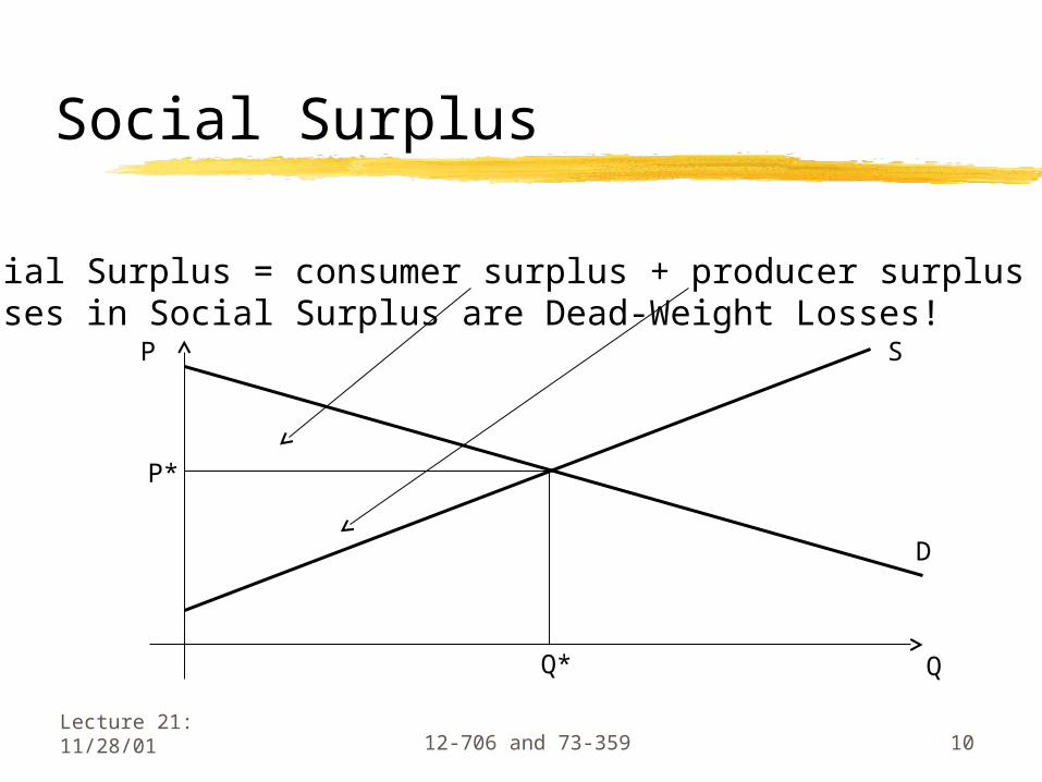
Value - travel time savings
Many studies seek to estimate VTTS Can then be used easily in CBAs
Book reminds us of Waters 1993 (56 studies) Many different methods used in studies Route, speed, mode, location choices Results as % of hourly wages not a $ amount Different rates for business and leisure Range of values (e.g. 50-100%)

Lecture 21: 11/28/01 12-706 and 73-359 23
Cost-Effectiveness Testing
Generally, use when: Considering externality effects or damages Alternatives give same result - eg ‘reduced
x’ Benefit-Cost Analysis otherwise difficult
Instead of finding NB, find “cheapest” Want greatest bang for the buck
Find cost “per benefit” (e.g. lives saved) Allows us to NOT include ‘social costs’

Lecture 21: 11/28/01 12-706 and 73-359 24
The CEA ratiosCE = C/E
Equals cost “per unit of effectiveness” e.g. dollars per lives saved, tons CO2 reduced Want to minimize CE (cheapest is best)
EC = E/C Effectiveness per unit cost e.g. Lives saved per dollar Want to maximize EC
No real difference between 2 ratios

Lecture 21: 11/28/01 12-706 and 73-359 25
Multiple Effectiveness
In Option 2, its not relevant to simply divide total costs (TC) by # deaths, # injuries, e.g. CE1 = TC/death, CE2 = TC/injury
Why? Misrepresents costs of each effectiveness
Instead, we need a method to allocate the costs (or to separate the benefits) so that we have CE ratios relevant to each effectiveness measure

Lecture 21: 11/28/01 12-706 and 73-359 26
WTP versus WTAEconomics implies that WTP should be
equal to ‘willingness to accept’Turns out people want MUCH MORE in
compensation for losing somethingWTA is factor of 4-15 higher than WTP!
Also see discrepancy shrink with experience WTP formats should be used in CVs Only can compare amongst individuals
Lecture 21: 11/28/01 12-706 and 73-359 27
Life Saving Metrics
Dollars/life savedDollars/life-year savedKnow how to calculate and interpret
each one (see notes from those lectures for details)
Know how to do annuity factors, etc.