1 Continuous Time Processes

1.1 Continuous Time Markov Chains

Let Xt be a family of random variables, parametrized by t ∈ [0,∞), withvalues in a discrete set S (e.g., Z). To extend the notion of Markov chain tothat of a continuous time Markov chain one naturally requires

P [Xs+t = j|Xs = i,Xsn = in, · · · , Xs1 = i1] = P [Xs+t = j|Xs = i] (1.1.1)

for all t > 0, s > sn > · · · > s1 ≥ 0 and i, j, ik ∈ S. This is the obviousanalogue of the Markov property when the discrete time variable l is replacedby a continuous parameter t. We refer to equation (1.1.1) as the Markovproperty and to the quantities P [Xs+t = j|Xs = i] as transition probabilitiesor matrices.

We represent the transition probabilities P [Xs+t = j|Xs = i] by a possiblyinfinite matrix P s

s+t. Making the time homogeneity assumption as in thecase of Markov chain, we deduce that the matrix P s

s+t depends only on thedifference s+ t− s = t and and therefore we simply write Pt instead of P s

s+t.Thus for a continuous time Markov chain, the family of matrices Pt (generallyan infinite matrix) replaces the single transition matrix P of a Markov chain.

In the case of Markov chains the matrix of transition probabilities after lunits of time is given by P l. The analogous statement for a continuous timeMarkov chain is

Ps+t = PtPs. (1.1.2)

This equation is known as the semi-group property. As usual we write P(t)ij

for the (i, j)th entry of the matrix Pt. The proof of (1.1.2) is similar tothat of the analogous statement for Markov chains, viz., that the matrix oftransition probabilities after l units of time is given by P l. Here the transitionprobability from state i to state j after t+ s units is given∑

k

P(t)ik P

(s)kj = P

(t+s)ij ,

which means (1.1.2) is valid. Naturally P = I.Just as in the case of Markov chains it is helpful to explicitly describe the

structure of the underlying probability space Ω of a continuous time Markovchain. Here Ω is the space of step functions on R+ with values in the state

1

space S. We also impose the additional requirement of right continuity onω ∈ Ω in the form

limt→a+

ω(t) = ω(a),

which means that Xt(ω), regarded as a function of t for each fixed ω, isright continuous function. This gives a definite time for transition fromstate i to state j in the sense that transition has occurred at time t meansXt−ε = i for ε > 0 and Xt+δ = j for δ ≥> 0 near t. One often requiresan initial condition X = i which means that we only consider the subsetof Ω consisting of functions ω with ω(0) = i. Each ω ∈ Ω is a path or a

realization of the Markov chain. In this context, we interpret P(t)ij as the

probability of the set of paths ω with ω(t) = j given that ω(0) = i.The concept of accessibility and communication of states carries over

essentially verbatim from the discrete case. For instance, state j is accessiblefrom state i if for some t we have P

(t)ij > 0, where P

(t)ij denotes the (i, j)th entry

of the matrix Pt. The notion of communication is an equivalence relation andthe set of states can be decomposed into equivalence classes accordingly.

The semi-group property has strong implications for the matrices Pt. Forexample, it immediately implies that the matrices Ps and Pt commute

PsPt = Ps+t = PtPs.

A continuous time Markov chain is determined by the matrices Pt. The factthat we now have a continuous parameter for time allows us to apply notionsfrom calculus to continuous Markov chains in a way that was not possible inthe discrete time chain. However, it also creates a number of technical issueswhich we treat only superficially since a thorough account would requireinvoking substantial machinery from functional analysis. We assume thatthe matrix of transition probabilities Pt is right continuous, and therefore

limh→0+

Pt = I. (1.1.3)

The limit here means entry wise for the matrix Pt. While no requirement ofuniformity relative to the different entries of the matrix Pt is imposed, we usethis limit also in the sense that for any vector v (in the appropriate functionspace) we have limt→0 vPt = v. We define the infinitesimal generator of the

2

continuous time Markov chain as the one-sided derivative

A = limh→0+

Ph − I

h.

A is a real matrix independent of t. For the time being, in a rather cavaliermanner, we ignore the problem of the existence of this limit and proceed asif the matrix A exists and has finite entries. Thus we define the derivative ofPt at time t as

dPtdt

= limh→0+

Pt+h − Pth

,

where the derivative is taken entry wise. The semi-group property impliesthat we can factor Pt out of the right hand side of the equation. We havetwo choices namely factoring Pt out on the left or on the right. Therefore weget the equations

dPtdt

= APt,dPtdt

= PtA. (1.1.4)

These differential equations are known as the Kolmogorov backward and for-ward equations respectively. They have remarkable consequences some ofwhich we will gradually investigate.

The (possibly infinite) matrices Pt are Markov or stochastic in the sensethat entries are non-negative and row sums are 1. Similarly the matrix A isnot arbitrary. In fact,

Lemma 1.1.1 The matrix A = (Aij) has the following properties:∑j

Aij = 0, Aii ≤ 0, Aij ≥ 0 for i 6= j.

Proof - Follows immediately from the stochastic property of Ph and thedefinition A = lim Ph−I

h. ♣

So far we have not exhibited even a single continuous time Markov chain.Using (1.1.4) we show that it is a simple matter to construct many examplesof stochastic matrices Pt, t ≥ 0.

Example 1.1.1 Assume we are given a matrix A satisfying the properties oflemma 1.1.1. Can we construct a continuous time Markov chain from A? IfA is an n× n matrix or it satisfies some boundedness assumption, we can in

3

principle construct Pt easily. The idea is to explicitly solve the Kolomogorov(forward or backward) equation. In fact if we replace the matrices Pt and Aby scalars, we get the differential equation dp

dt= ap which is easily solved by

p(t) = Ceat. Therefore we surmise the solution Pt = CetA for the Kolmogorovequations where we have defined the exponential of a matrix B as the infiniteseries

eB =∑j

Bj

j!(1.1.5)

where B = I. Substituting tA for B and differentiating formally we see thatCetA satisfies the Kolmogorov equation for any matrix C. The requirementP = I (initial condition) implies that we should set C = I, so that

Pt = etA (1.1.6)

is the desired solution to the Kolmogorov equation. Some boundedness as-sumption on A would ensure the existence of etA, but we shall not dwell onthe issue of the existence and meaning of eB which cannot be adequatelytreated in this context. An immediate implication of (1.1.6) is that

detPt = etTrA > 0,

assuming the determinant and trace exist. For a discrete time Markov chaindetP can be negative. It is necessary to verify that the matrices Pt fulfill therequirements of a stochastic matrix. Proceeding formally (or by assumingthe matrices in question are finite) we show that if the matrix A fulfills therequirements of lemma 1.1.1, then Pt is a stochastic matrix. To prove this letA and B be matrices with row sums equal to zero, then the sum of entriesof the ith row of AB is (formally)∑

k

∑j

AijBjk =∑j

Aij∑k

Bjk = 0.

To prove non-negativity of the entries we make use of the formula (familiarfrom calculus for A a scalar)

etA = limn→∞

(I +tA

n)n. (1.1.7)

It is clear that for n sufficiently large the entries of the N ×N matrix I + tAn

are non-negative (boundedness condition on entries of A) and consequentlyetA is a non-negative matrix. ♠

4

Nothing in the definition of a continuous time Markov chain ensures theexistence of the infinitesimal generator A. In fact it is possible to constructcontinuous time Markov chains with diagonal entries of A being −∞. Intu-itively this means the transition out of a state may be instantaneous. Formany Markov chains appearing in the analysis of problems of interest donot allow of instantaneous transitions. We eliminate this possibility by therequirement

P [Xs+h = i for all h ∈ [0, ε) | Xs = i] = 1− λis+ o(ε), (1.1.8)

as ε→ 0. Here λi is a non-negative real number and the notation g(ε) = o(ε)means

limε→0

g(ε)

ε= 0.

Let T denote the time of first transition out of state i where we assumeX = 0. Excluding the possibility of instantaneous transition out of i, therandom variable T is necessarily memoryless for otherwise the Markov prop-erty, whereby assuming the knowledge of the current state the knowledge ofthe past is irrelevant to predictions about the future, will be violated. It is astandard result in elementary probability that the only memoryless continu-ous random variables are exponentials. Recall that the distribution functionfor the exponential random variable T with parameter λ is given by

P [T < t] =

1− e−λt, if t 0;0, if t ≤ 0.

The mean and variance of T are 1λ. It is useful to allow the possibility

λi = ∞ which means that the state i is absorbing, i.e., no transition out of itis possible. The exponential nature of the transition time is compatible withthe requirement (1.1.8). With this assumption one can rigorously establishexistence of the infinitesimal generator A, but this is just a technical matterwhich we shall not dwell on.

While we have eliminated the case of instantaneous transitions, there isnothing in the definitions that precludes having an infinite number transi-tions in a finite interval of time. It in fact a simple matter to constructcontinuous time Markov chains where infinitely many transitions in finiteinterval occur with positive probability. In fact, since the expectation of an

5

exponential random variable with parameter λ is 1λ, it is intuitively clear

that if λi’s increase sufficiently fast we should expect infinitely transitions ina finite interval. In order to analyze this issue more closely we consider afamily T1, T2, . . . of independent exponential random variables with Tk hav-ing parameter λk. Then we consider the infinite sum

∑k Tk. We consider the

events

[∑k

Tk <∞] and [∑k

Tk = ∞].

The first event means there are infinitely many transitions in a finite intervalof time, and the second is the complement. It is intuitively clear that ifthe rates λk increases sufficiently rapidly we should expect infinitely manytransitions in a finite interval, and conversely, if the rates do not increasetoo fast then only finitely many transitions are possible i finite time. Moreprecisely, we have

Proposition 1.1.1 Let T1, T2, . . . be independent exponential random vari-ables with parameters λ1, λ2, . . .. Then

∑k

1λk

< ∞ (resp.∑k

1λk

< ∞)

implies P [∑k Tk <∞] = 1 (resp. P [

∑k Tk = ∞] = 1).

Proof - We have

E[∑k

Tk] =∑k

1

λk,

and therefore if∑k

1λk

< ∞ then P [∑Tk = ∞] = 0 which proves the first

assertion. To prove the second assertion note that

E[e−∑

Tk ] =∏k

E[e−Tk ].

Now

E[e−Tk ] =∫ ∞

P [−Tk > log s]ds

=∫ ∞

P [Tk < − log s]ds

=λk

1 + λk.

6

Therefore, by a standard theorem on infinite products1,

E[e−∑

Tk ] =∏ 1

1 + 1λk

= 0.

Since e−∑

Tk is a non-negative random variable, its expectation can be 0 onlyif∑Tk = ∞ with probability 1. ♣

Remark 1.1.1 It may appear that the Kolmogorov forward and backwardequations are one and the same equation. This is not the case. While A andPt formally commute, the domains of definition of the operators APt andPtA are not necessarily identical. The difference between the forward andbackward equations becomes significant, for instance, when dealing with cer-tain boundary conditions where there is instantaneous return from boundarypoints (or points at infinity) to another state. However if the infinitesimalgenerator A has the property that the absolute values of the diagonal entriessatisfy a uniform bound |Aii| < c, then the forward and backward equationshave the same solution Pt with P = I. In general, the backward equationhas more solutions than the forward equation and its minimal solution is alsothe solution of the forward equation. Roughly speaking, this is due to thefact that A can be an unbounded operator, while Pt has a smoothing effect.An analysis of such matters demands more technical sophistication than weare ready to invoke in this context. ♥

Remark 1.1.2 The fact that the series (1.1.5) converges is is easy to showfor finite matrices or under some bounded assumption on the entries of thematrix A. If the entries Ajk grow rapidly with k, j, then there will be conver-gence problems. In manipulating exponentials of (even finite) matrices oneshould be cognizant of the fact that if AB 6= BA then eA+B 6= eAeB. On theother hand if AB = BA then eA+B = eAeB as in the scalar case. ♥

Recall that the stationary distribution played an important role in thetheory of Markov chains. For a continuous time Markov chain we similarlydefine the stationary distribution as a row vector π = (π1, π2, · · ·) satisfying

πPt = π for all t ≥ 0,∑

πj = 1, πj ≥ 0. (1.1.9)

1Let ak be a sequence of positive numbers, then the infinite product∏

(1 + ak)−1

diverges to 0 if and only if∑

ak = ∞. The proof is by taking logarithms and expanding thelog and can be found in many books treating infinite series and products, e.g. Titchmarsh- Theory of Functions, Chapter 1.

7

The following lemma re-interprets πPt = π in terms of the infinitesimalgenerator A:

Lemma 1.1.2 The condition πPt = π is equivalent to πA = 0.

Proof - It is immediate that the condition πPt − π = 0 implies πA = 0.Conversely, if πA = 0, then the Kolmogorov backward equation implies

d(πPt)

dt= π

dPtdt

= πAPt = 0.

Therefore πPt is independent of t. Substituting t = 0 we obtain πPt = πP =π as required. ♣

Example 1.1.2 We apply the above considerations to an example fromqueuing theory. Assume we have a server which can service one customerat a time. The service times for customers are independent identically dis-tributed exponential random variables with parameter µ. The arrival timesare also assumed to be independent identically identically distributed expo-nential random variables with parameter λ. The customers waiting to beserviced stay in a queue and we let Xt denote the number of customers inthe queue at time t. Our assumption regarding the exponential arrival timesimplies

P [X(t+ h) = k + 1 | X(t) = k] = λh+ o(h).

Similarly the assumption about service times implies

P [X(t+ h) = k − 1 | X(t) = k] = µh+ o(h).

It follows that the infinitesimal generator of Xt is

A =

−λ λ 0 0 0 · · ·µ −(λ+ µ) λ 0 0 · · ·0 µ −(λ+ µ) λ 0 · · ·0 0 µ −(λ+ µ) λ · · ·...

......

......

. . .

The system of equations πA = 0 becomes

−λπ + µπ1 = 0, · · · , λπi−1 − (λ+ µ)πi + µπi+1 = 0, · · ·

8

This system is easily solved to yield

πi = (λ

µ)iπ.

For λ < µ we obtain

πi = (1− λ

µ)(λ

µ)i.

as the stationary distribution. ♠

The semi-group property (1.1.2) implies

P(t)ii ≥

(P

tnii

)n.

The continuity assumption (1.1.3) implies that for sufficiently large n, P( t

n)

ii >0 and consequently

P(t)ii > 0, for t > 0.

More generally, we have

Lemma 1.1.3 The diagonal entries P(t)ii > 0, and off-diagonal entries P

(t)ij ,

i 6= j, are either positive for all t > 0 or vanish identically. The entries ofthe matrix Pt are right continuous as functions of t.

Proof - We already know that P(t)jj > 0 for all t. Now assume P

(t)ij = 0 where

i 6= j. Then for α, β > 0, α+ β = 1 we have

P(t)ij ≥ P

(αt)ii P

(βt)ij .

Consequently P(βt)ij = 0 for all 0 < β < 1. This means that if P

(t)ij = 0, the

P(s)ij = 0 for all s ≤ t. The conclusion that P

(s)ij = 0 for all s is proven later

(see corollary 1.4.1). The continuity property (1.1.3)

limh→0+

Pt+h = Pt

(limh→0+

Ph

)= Pt.

implies right continuity of P(t)ij . ♣

Note that in the case of a finite state Markov chain Pt has convergentseries representation Pt = etA, and consequently the entries P

(t)ij are analytic

functions of t. An immediate consequence is

9

Corollary 1.1.1 If all the states of a continuous time Markov chain commu-nicate, then the Markov chain has the property that P

(t)ij > 0 for all i, j ∈ S

(and all t > 0). In particular, if S is finite then all states are aperiodic andrecurrent.

In view of the existence of periodic states in the discrete time case, thiscorollary stands in sharp contrast to the latter situation. The existenceof the limiting value of liml→∞ P l for a finite state Markov chain and itsimplication regarding long term behavior of the Markov chain was discussedin §1.4. The same result is valid here as well, and the absence of periodicstates for continuous Markov chains results in a stronger proposition. In fact,we have

Proposition 1.1.2 Let Xt be a finite state continuous time Markov chainand assume all states communicate. Then Pt has a unique stationary distri-bution π = (π1, π2, · · ·), and

limt→∞

P(t)ij = πi.

Proof - It follows from the hypotheses that for some t > 0 all entries ofPt are positive, and consequently for all t > 0 all entries of Pt are positive.Fix t > 0 and let Q = Pt be the transition matrix of a finite state (discretetime) Markov chain. limlQ

l is the rank one matrix each row of which is thestationary distribution of the Markov chain. This limit is independent ofchoice of t > 0 since

liml→∞

Pt(Ps)l = lim

l→∞(Ps)

l

for every s > 0. ♣

10

EXERCISES

Exercise 1.1.1 A hospital owns two identical and independent power gen-erators. The time to breakdown for each is exponential with parameter λ andthe time for repair of a malfunctioning one is exponential with parameter µ.Let X(t) be the Markov process which is the number of operational genera-tors at time t ≥ 0. Assume X(0) = 2. Prove that the probability that bothgenerators are functional at time t > 0 is

µ2

(λ+ µ)2+λ2e−2(λ+µ)t

(λ+ µ)2+

2λµe−(λ+µ)t

(λ+ µ)2.

Exercise 1.1.2 Let α > 0 and consider the random walk Xn on the non-negative integers with a reflecting barrier at 0 defined by

pi i+1 =α

1 + α, pi i−1 =

1

1 + α, for i ≥ 1.

1. Find the stationary distribution of this Markov chain for α < 1.

2. Does it have a stationary distribution for α ≥ 1?

Exercise 1.1.3 (Continuation of exercise 1.1.2) - Let Y, Y1, Y2, · · · be inde-pendent exponential random variables with parameters µ, µ1, µ2, · · · respec-tively. Now modify the Markov chain Xn of exercise 1.1.2 into a Markovprocess by postulating that the holding time in state j before transition toj − 1 or j + 1 is random according to Yj.

1. Explain why this gives a Markov process.

2. Find the infinitesimal generator of this Markov process.

3. Find its stationary distribution by making reasonable assumption onµj’s and α < 1.

11

1.2 Inter-arrival Times and Poisson Processes

Poisson processes are perhaps the most basic examples of continuous timeMarkov chains. In this subsection we establish their basic properties. To con-struct a Poisson process we consider a sequence W1,W2, . . . of iid exponentialrandom variables with parameter λ. Wj’s are called inter-arrival times. SetT1 = W1, T2 = W +W1 and Tn = Tn−1 +Wn. Tj’s are called arrival times.Now define the Poisson process Nt with parameter λ as

Nt = maxn | W1 +W2 + · · ·+Wn ≤ t (1.2.1)

Intuitively we can think of certain events taking place and every time theevent occurs the counter Nt is incremented by 1. We assume N0 and thetimes between consecutive events, i.e., Wj’s, being iid exponentials with thesame parameter λ. Thus Nt is the number of events that have taken placeuntil time t. The validity of the Markov property follows from the construc-tion of Nt and the exponential nature of the inter-arrival times, so that thePoisson process is a continuous time Markov chain. It is clear that Nt isstationary in the sense that Ns+t −Ns has the same distribution as Nt.

The arrival and inter-arrival times can be recovered from Nt by

Tn = supt | Nt ≤ n− 1, (1.2.2)

and Wn = Tn − Tn−1. One can similarly construct other counting processesby considering sequences of independent random variables W1,W2, . . . anddefining Tn and Nt just as above. The assumption that Wj’s are exponentialis necessary and sufficient for the resulting process to be Markov. Whatmakes Poisson processes special among Markov counting processes is thatthe inter-arrival times have the same exponential law. The case where Wj’sare not necessarily exponential (but iid) is very important and will be treatedin connection with renewal theory later.

The underlying probability space Ω for a Poisson process is the space non-decreasing right continuous step function functions such that at each point ofdiscontinuity a we have step function ϕ where at each point of discontinuitya ∈ R+

ϕ(a)− limt→a−

ϕ(t) = 1,

reflecting the fact that from state n only transition to state n+1 is possible.

12

To analyze Poisson processes we begin by calculating the density func-tion for Tn. Recall that the distribution of a sum of independent exponentialrandom variables is computed by convolving the corresponding density func-tions (or using Fourier transforms to convert convolution to multiplication.)Thus it is a straightforward calculation to show that Tn = W1 + · · ·+Wn hasdensity function

f(n,µ)(x) =

µe−µx(µx)n−1

(n−1)!for x ≥ 0;

0 for x < 0.(1.2.3)

One commonly refers to f(n,µ) as Γ density with parameters (n, µ), so thatTn has Γ distribution with parameters (n, µ). From this we can calculate thedensity function for Nt, for given t > 0. Clearly Tn+1 ≤ t ⊂ Tn ≤ t andthe event Nt = n is the complement of Tn+1 ≤ t in Tn ≤ t. Thereforeby (1.2.3) we have

P [Nt = n] =∫ t

f(n,µ)(x)dx−

∫ t

f(n+1,µ)(x)dx =

e−µt(µt)n

n!. (1.2.4)

Hence Nt is a Z+-valued random variable whose distribution is Poisson withparameter µt, hence the terminology Poisson process. This suggests that wecan interpret the Poisson process Nt as the number of arrivals at a server inthe interval of time [0, t] where the assumption is made that the number ofarrivals is a random variable whose distribution is Poisson with parameterµt.

In addition to stationarity Poisson processes have another remarkableproperty. Let 0 ≤ t1 < t2 ≤ t3 < t4, then the random variables Nt2 −Nt1 and Nt4 − Nt3 are independent. This property is called independenceof increments of Poisson processes. The validity of this property can beunderstood intuitively without a formal argument. The essential point is thatthe inter-arrival times have the same exponential distribution and thereforethe number of increments in the interval (t3, t4) is independent of how manytransitions have occurred up to time t3 an in particular independent of thenumber of transitions in the interval (t1, t2). A more formal proof will alsofollow from our analysis of Poisson processes.

To compute the infinitesimal generator of the Poisson process we notethat in view of (1.2.4) for h > 0 small we have

P [Nh = 0]− 1 = −µh+ o(h), P [Nh = 1] = µh+ o(h), P [Nh ≥ 2] = o(h).

13

It follows that the infinitesimal generator of the Poisson process Nt is

A =

−µ µ 0 0 0 · · ·0 −µ µ 0 0 · · ·0 0 −µ µ 0 · · ·0 0 0 −µ µ · · ·...

......

......

. . .

(1.2.5)

To further analyze Poisson processes we recall the following elementaryfact:

Lemma 1.2.1 Let Xi be random variables with uniform density on [0, a]with their indices re-arranged so that X1 < X2 < · · · < Xm (called orderstatistics. The joint distribution of (X1, X2, · · · , Xn) is

f(x1, · · · , xm) =

m!am , if x1 ≤ x2 ≤ · · · ≤ xm;0, otherwise.

Proof - The m! permutations decompose [0, a]m into m! subsets accordingto

xi1 ≤ xi2 ≤ · · · ≤ xim

from which the required result follows.Let X1, · · · , Xm be (continuous) random variables with density function

f(x1, · · · , xm)dx1 · · · dxm. Let Y1, · · · , Ym be random variables such that Xj’sand Yj’s are related by invertible transformations. Thus the joint density ofY1, · · · , Ym is given by h(y1, · · · , ym)dy1 · · · dym. The density functions f andh are then related by

h(y1, · · · , ym) = f(x1(y1, · · · , ym), · · · , xm(y1, · · · , ym))|∂(x1, · · · , xm)

∂(y1, · · · , ym)|,

where ∂(x1,···,xm)∂(y1,···,ym)

denotes the the familiar Jacobian determinant from calculusof several variables. In the particular case that Xj’s and Yj’s are related byan invertible linear transformation

Xi =∑∑

j

AijYj

14

we obtain

h(y1, · · · , ym) = detAf(∑

A1iyi, · · · ,∑

Amiyi).

We now apply these general considerations to calculate the conditional den-sity of T1, · · · , Tm given Nt = m.

Since W1, · · · ,Wm are independent exponentials with parameter µ, theirjoint density is

f(w1, · · · , wm) = µme−µ(w1+···+wm) for wi ≥ 0.

Consider the linear transformation

t1 = w1, t2 = w1 + w2, · · · , tm = w1 + · · ·+ wm

Then the joint density of random variables T1, T2, · · · , Tm+1 is

h(t1, · · · , tm+1) = µm+1e−µtm+1 .

Therefore to calculate

P [Am | Nt = m] =P [Am, Nt = m]

Nt = m,

where Am denotes the event

Am = 0 < T1 < t1 < T2 < t2 < · · · < tm−1 < Tm < tm < t < Tm+1

we evaluate the numerator of the right hand side by noting that the conditionNt = m is implied by the requirement Tm < tm < t <. Now

P [Am] =∫Uµm+1eµtm+1ds1 · · · dsm+1

where U is the region

U : (s1, · · · , sm+1) such that 0 < s1 < t1 < s2 < t2 < · · · < sm < tm < t < sm+1.

Carrying out the simple integration we obtain

P [Am] = µmt1(t2 − t1) · · · (tm − tm−1)e−µt

15

Therefore

P [Am | Nt = m] = t1(t2 − t1) · · · (tm − tm−1)m!

tm. (1.2.6)

To obtain the conditional joint density of T1, · · · , Tm given Nt = m we applythe differential operator ∂m

∂t1···∂tm to (1.2.6) to obtain

fT |N(t1, · · · , tm) =m!

tm, 0 ≤ t1 < t2 < · · · < tm ≤ t. (1.2.7)

We deduce the following remarkable fact:

Proposition 1.2.1 With the above notation and hypotheses, the conditionaljoint density of T1, · · · , Tm given Nt = m is identical with that of the orderstatistics of m uniform random variables from [0, t].

Proof - Follows from lemma 1.2.1 and (1.2.7). ♣.A simple consequence of Proposition 1.2.1 is a proof of the independence

of increments for a Poisson process. To do so let t1 < t2 ≤ t3 < t4, U =Nt2 −Nt1 and V = Nt4 −Nt3 . Then

E[ξUηV ] = E[E[ξUηV | Nt4 ]]

Recall from elementary probability that conditioned on Nt4 = M , the timest1, t2 and t3 are uniformly distributed in [0, t4]. Therefore the conditionalexpectation E[ξUηV | Nt4 ] is easily computed (see example ??)

E[ξUηV | Nt4 ] =[(t2 − t1t4

)ξ +

(t4 − t3t4

)η +

(t1 + t3 − t2

t4

)]M(1.2.8)

Since for fixed t, Nt is a Poisson random variable with parameter µt, we cancalculate the outer expectation to obtain

E[ξUηV ] = eµ[ξ(t2−t1)+η(t4−t3)+(t1+t3−t2−t4)]

= eµ(t2−t1)(ξ−1)eµ(t4−t3)(η−1)

= E[ξU ]E[ηV ],which proves the independence of increments of a Poisson process. Summa-rizing

Proposition 1.2.2 The Poisson process Nt with parameter µ has the fol-lowing properties:

16

1. For fixed t > 0, Nt is a Poisson random variable with parameter µt;

2. Nt is stationary (i.e., Ns+t −Ns has the same distribution as Nt) andhas independent increments;

3. The infinitesimal generator of Nt is given by (1.2.5).

Property (3) of proposition 1.2.2 follows from the first two which in factcharacterize Poisson processes. From the infinitesimal generator (1.2.5) onecan construct the transition probabilities Pt = etA.

There is a general procedure for constructing continuous time Markovchains out of a Poisson process and a (discrete time) Markov chain. Theresulting Markov chains are often considerably easier to analyze and behavesomewhat like the finite state continuous time Markov chains. It is cus-tomary to refer to these processes as Markov chains subordinated to Poissonprocesses. Let Zn be a (discrete time) Markov chain with transition ma-trix K, and Nt be a Poisson process with parameter µ. Let S be the statespace of Zn. We construct the continuous time Markov chain with statespace S by postulating that the number of transitions in an interval [s, s+ t)is given by Nt+s − Ns which has the same distribution as Nt. Given thatthere are n transitions in the interval [s, s + t), we require the probabilityP [Xs+t = j | Xs = i, Nt+s −Ns = n] to be

P [Xs+t = j | Xs = i, Nt+s −Ns = n] = K(n)ij .

Let K = I, then the transition probability P(t)ij for Xt is given by

P(t)ij =

∞∑n=

e−µt(µt)n

n!K

(n)ij . (1.2.9)

The infinitesimal generator is easily computed by differentiating (1.2.9) att = 0:

A = µ(−I +K). (1.2.10)

From the Markov property of the matrix K it follows easily that the infiniteseries expansion of etA converges and therefore Pt = etA is rigorously defined.The matrix Q of lemma 1.4.1 can also be expressed in terms of the Markovmatrix K. Assuming no state is absorbing we get (see corollary 1.4.2)

Qij =

0, if i = j;Kij

1−Kii, otherwise. (1.2.11)

17

Note that if (1.2.10) is satisfied then from A we obtain a continuous timeMarkov chain subordinate to a Poisson process.

18

EXERCISES

Exercise 1.2.1 For the two state Markov chain with transition matrix

K =(p qp q

),

show that the continuous time Markov chain subordinate to the Poisson pro-cess of rate µ has trasnsition matrix

Pt =(p+ qe−µt q − qe−µt

p− pe−µt q + pe−µt

)

1.3 The Kolomogorov Equations

To understand the significance of the Kolmogorov equations we analyze asimple continuous time Markov chain. The method is applicable to manyother situations and it is most easily demonstrated by an example. Considera simple pure birth process by which we mean we have a (finite) numberof organisms which independently and randomly split into two. We let Xt

denote the number of organisms at time t and it is convenient to assume thatX = 1. The law for splitting of a single organism is given by

P [splitting in h units of time] = λh+ o(h)

for h > 0 a small real number. This implies that the probability that a singleorganism splits more than once in h units of time is o(h). Now suppose thatwe have n organisms and Aj denote the event that organism number j splits(at least once) and A be the event that in h units of time there is exactlyone split. Then

P [A] =∑j

P [Aj]−∑i<j

P [Ai ∩ Aj] +∑i<j<k

P [Ai ∩ Aj ∩ Ak]− · · ·

The probability of each of the events Ai ∩ Aj, Ai ∩ Aj ∩ Ak etc. is clearlyo(h) for h > 0 small. Therefore

P [A] = nλh+ o(h). (1.3.1)

Note that the exact value of the terms incorporated into o(h) is quite com-plicated. We shall see that in spite of ignoring these complicated terms, we

19

can recover exact information about our continuous time Markov chain byusing Kolmogorov forward equation. Let B be the event that in h units oftime there are at least two splits, and C the event that there are no split ofthe n organisms. Then

P [B] = o(h), P [C] = 1− λnh+ o(h). (1.3.2)

Equations (1.3.1) and (1.3.2) imply that the infinitesimal generator A of thecontinuous time Markov chain Xt is

A =

−λ λ 0 0 0 · · ·0 −2λ 2λ 0 0 · · ·0 0 −3λ 3λ 0 · · ·...

......

......

. . .

For any initial distribution π = (π1, π

2, · · ·) let q(t) = (q1(t), q2(t), · · ·)

be the row vector q(t) = πPt which describes the distribution of states attime t. In fact,

qk(t) = P [Xt = k | X = π].

Thus a basic problem about the Markov chain Xt is the calculation of E[Xt]or more generally of the generating function

FX(t, ξ) = E[ξXt ] =∑k=1

P [Xt = k]ξk.

We now use Kolomogorov’s forward equation to solve this problem. From(1.1.4) we obtain

dq(t)

dt= π

dPtdt

= πPtA = q(t)A.

Expanding the qtA we obtain

dqk(t)

dt= −kλqk(t) + (k − 1)λqk−1(t). (1.3.3)

With a little straightforward book-keeping, one shows that (1.3.3) implies

∂FX∂t

= λ(ξ2 − ξ)∂FX∂ξ

. (1.3.4)

20

The fact that FX a linear partial differential equation makes the calcula-tion of E[Xt] very simple. In fact, since E[Xt] = ∂FX

∂ξevaluated at ξ = 1−,

we differentiate both sides of (1.3.4) with respect to ξ, change the order ofdifferentiation relative to ξ and t on the left side, and set ξ = 1 to obtain

dE[Xt]

dt= λE[Xt]. (1.3.5)

The solution to this ordinary differential equation is Ceλt and the constantC is determined by the initial condition X = 1 to yield

E[Xt] = eλt.

The partial differential equation (1.3.4) tells us considerably more thanjust the expectation of Xt. The basic theory of a single linear first orderpartial differential equation is well understood. Recall that the solution to afirst order ordinary differential equation is uniquely determined by specifyingone initial condition. Roughly speaking, the solution to a linear first orderpartial differential equation in two variables is uniquely determined by spec-ifying a function of one variable. Let us see how this works for our equation(1.3.4). For a function g(s) of a real variable s we want to substitute for sa function of t and ξ such that (1.3.4) is necessarily valid regardless of thechoice of g. If for s we substitute λt+ φ(ξ), then by the chain rule

∂g(λt+ φ(ξ))

∂t= λg′(λt+ φ(ξ)),

∂g(λt+ φ(ξ))

∂ξ= φ′(ξ)g′(λt+ φ(ξ)).

where g′ denote the derivative of the function g. Therefore if φ is suchthat φ′(ξ) = 1

ξ2−ξ , then, regardless of what function we take for g, equation

(1.3.4) is satisfied by g(λt + φ(ξ)). There is an obvious choice for φ namelythe function

φ(ξ) =∫ ξ

12

du

u2 − u= log

ξ

1− ξ,

for 0 < ξ < 1. (The lower limit of the integral is immaterial and 12

is fixedfor convenience.) Now we incorporate the initial condition X = 1 which interms of the generating function FX means FX(0, ξ) = ξ. In terms of g thistranslates into

g(log1− ξ

ξ) = ξ.

21

That is, g should be the inverse to the mapping ξ → log 1−ξξ

. It is easy tosee that

g(s) =es

1 + es

is the required function. Thus we obtain the expression

FX(t, ξ) =ξ

ξ + (1− ξ)e−λt(1.3.6)

for the probability generating function of Xt. If we change the initial condi-tion to X = N , then the generating function becomes

FX(ξ, t) =ξN

[ξ + (1− ξ)e−λt]N.

From this we deduce

P(t)Nj = e−Nλt

(j − 1

N − 1

)(1− e−λt)N−j

for the transition probabilities. The method of derivation of (1.3.6) is re-markable and instructive. We made essential use of the Kolmogorov forwardequation in obtaining a linear first order partial differential equation for theprobability generating function. This was possible because we have an infi-nite number of states and the coefficients of qk(t) and qk−1(t) in (1.3.3) werelinear in k. If the dependence were quadratic in k, probably we could haveobtained a partial differential equation which had order two relative to thevariable ξ and the situation would have been more complex. The fact thatwe have an explicit differential equation for the generating function gave usa fundamental new tool for understanding it. In the exercises this methodwill be further demonstrated.

Example 1.3.1 The birth process described above can be easily generalizedto a birth-death process by introducing a positive parameter µ > 0 andreplacing equations (1.3.1) and (1.3.2) with the requirement

P [Xt+h = n+ a | Xt = n] =

nµh+ o(h), if a = −1;nλh+ o(h), if a = 1;o(h), if |a| > 1.

(1.3.7)

22

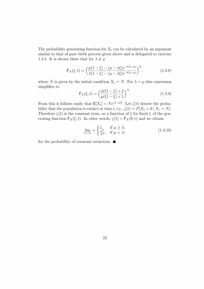
The probability generating function for Xt can be calculated by an argumentsimilar to that of pure birth process given above and is delegated to exercise1.3.5. It is shown there that for λ 6= µ

FX(ξ, t) =(µ(1− ξ)− (µ− λξ)e−t(λ−µ)

λ(1− ξ)− (µ− λξ)e−t(λ−µ)

)N. (1.3.8)

where N is given by the initial condition X = N . For λ = µ this expressionsimplifies to

FX(ξ, t) =(µt(1− ξ) + ξ

µt(1− ξ) + 1

)N. (1.3.9)

From this it follows easily that E[Xt] = Ne(λ−µ)t. Let ζ(t) denote the proba-bility that the population is extinct at time t, i.e., ζ(t) = P [Xt = 0 |X = N ].Therefore ζ(t) is the constant term, as a function of ξ for fixed t, of the gen-erating function FX(ξ, t). In other words, ζ(t) = FX(0, t) and we obtain

limt→∞

=

1, if µ ≥ λ;µN

λN , if µ < λ;(1.3.10)

for the probability of eventual extinction. ♠

23

EXERCISES

Exercise 1.3.1 (M/M/1 queue) A server can service only one customer at atime and the arriving customers form a queue according to order of arrival.Consider the continuous time Markov chain where the length of the queueis the state space, the time between consecutive arrivals is exponential withparameter µ and the time of service is exponential with parameter λ. Showthat the matrix Q = (Qij) of lemma 1.4.1 is

Qij =

µ

µ+λ, if j = i+ 1;

λµ+λ

, if j = i− 1;0, otherwise.

Exercise 1.3.2 The probability that a central networking system receives acall in the time period (t, t + h) is λh + o(h) and calls are received inde-pendently. The service time for the calls are independent and identicallydistributed each according to the exponential random variable with parameterµ. The service times are also assumed independent of the incoming calls.Consider the Markov process X(t) with state space the number of calls beingprocessed by the server. Show that the infinitesimal generator of the Markovprocess is the infinite matrix

−λ λ 0 0 0 · · ·µ −(λ+ µ) λ 0 0 · · ·0 2µ −(λ+ 2µ) λ 0 · · ·...

......

......

. . .

Let FX(ξ, t) = E(ξX(t)) denote the generating function of the Markov process.Show that FX satisfies the differential equation

∂FX∂t

= (1− ξ)[−λFX + µ∂FX∂ξ

].

Assuming that X(0) = m, use the differential equation to show that

E[X(t)] =λ

µ(1− e−µt) +me−µt.

24

Exercise 1.3.3 (Continuation of exercise 1.3.2) - With the same notationas exercise 1.3.2, show that the substitution

FX(ξ, t) = e−λ(1−ξ)

µ G(ξ, t)

gets rid of the term involving FX on the right hand side of the differentialequation for FX . More precisely, it transforms the differential equation forFX into

∂G

∂t= µ(1− ξ)

∂G

∂ξ.

Can you give a general approach for solving this differential equation? Verifythat

FX(ξ, t) = e−λ(1−ξ)(1−e−µt)/µ[1− (1− ξ)e−µt]m

is the desired solution to equation for FX .

Exercise 1.3.4 The velocities Vt of particles in a quantized field are assumedto take only discrete values n + 1

2, n ∈ Z+. Under the influence of the field

and mutual interactions their velocities can change by at most one unit andthe probabilities for transitions are given by

P [Vt+h = m+1

2| Vt = n+

1

2] =

(n+ 1

2)h+ o(h), if m = n+ 1;

1− (2n+ 1)h+ o(h), if m = n;(n− 1

2)h+ o(h), if m = n− 1.

Let FV (ξ, t) be the probability generating function

FV (ξ, t) =∞∑n=0

P [Vt = n+1

2]ξn.

Show that

∂FV∂t

= (1− ξ)2∂FV∂s

− (1− ξ)FX .

Assuming that V = 0 deduce that

FV (ξ, t) =1

1 + t− ξt.

25

Exercise 1.3.5 Consider the birth-death process of example 1.3.1

1. Show that the generating function FX(ξ, t) = E[ξXt ] satisfies the partialdifferential equation

∂FX∂t

= (λξ − µ)(ξ − 1)∂FX∂ξ

,

with the initial condition FX(ξ, 0) = ξN .

2. Deduce the validity of (1.3.7) and (1.3.8).

3. Show that

Var[Xt] = Nλ+ µ

λ− µe(λ−µ)t(e(λ−µ)t − 1).

4. Let N = 1 and Z denote the time of the extinction of the process. Showthat for λ = µ , E[Z] = ∞.

5. Show that µ > λ we have

E[Z | Z <∞] =1

λlog

µ

µ− λ.

6. Show that µ < λ we have

E[Z | Z <∞] =1

µlog

µ

µ− λ.

(Use the fact that

E[Z] =∫ ∞

P [Z > t]dt =

∫ ∞

[1− FX(0, t)]dt,

to calculate E[Z | Z <∞].)

26

1.4 Discrete vs. Continuous Time Markov Chains

In this subsection we show how to assign a discrete time Markov chain to onewith continuous time, and how to construct continuous time Markov chainsfrom a discrete time one. We have already introduced the notions of Markovand stopping times for for Markov chains, and we can easily extend them tocontinuous time Markov chains. Intuitively a Markov time for the (possiblycontinuous time) Markov chain is a random variable T such that the event[T ≤ t] does not depend on Xs for s > t. Thus a Markov time T has theproperty that if T (ω) = t then T (ω′) = t for all paths which are identicalwith ω for s ≤ t. For instance, for a Markov chain Xl with state space Zand X = 0 let T be the first hitting time of state 1 ∈ Z. Then T is aMarkov time. If T is Markov time for the continuous time Markov chain Xt,the fundamental property of Markov time, generally called Strong MarkovProperty, is

P [XT+s = j | Xt, t ≤ T ] = P(s)XT j

(1.4.1)

This reduces to the Markov property if we take T to be a constant. Tounderstand the meaning of equation (1.4.1), consider Ωu = ω | T (ω) = uwhere u ∈ R+ is any fixed positive real number. Then the left hand side of(1.4.1) is the conditional probability of the set of paths ω that after s unitsof time are in state j given Ωu and Xt for t ≤ u = T (ω). The right handside states that the information Xt for t ≤ u is not relevant as long we knowthe states for which T (ω) = u, and this probability is the probability of thepaths which after s units of time are in state j assuming at time 0 they werein a state determined by T = u. One can also loosely think of the strongMarkov property as allowing one to reparametrize paths so that all the pathswill satisfy T (ω) = u at the same constant time T and then the standardMarkov property will be applicable. Examples that we encounter will clarifythe meaning and significance of this concept. The validity of (1.4.1) is quiteintuitive, and one can be convinced of its validity by looking at the set ofpaths with the required properties and using the Markov property. It issometimes useful to make use of a slightly more general version of the strongMarkov property where a function of the Markov time is introduced. Ratherthan stating a general theorem, its validity in the context where it is usedwill be clear.

The notation Ei[Z] where the random variable Z is a function of of thecontinuous time Markov chain Xt means that we are calculating conditional

27

expectation conditioned on X = i. Naturally, one may replace the subscript

i by a random variable to accommodate a different conditional expectation.Of course, instead of a subscript one may write the conditioning in the usualmanner E[? | ?]. The strong Markov property in the context of conditionalexpectations implies

E[g(XT+s) | Xu, u ≤ T ] = EXT[g] = E[

∑j∈S

P(s)XT j

g(j)]. (1.4.2)

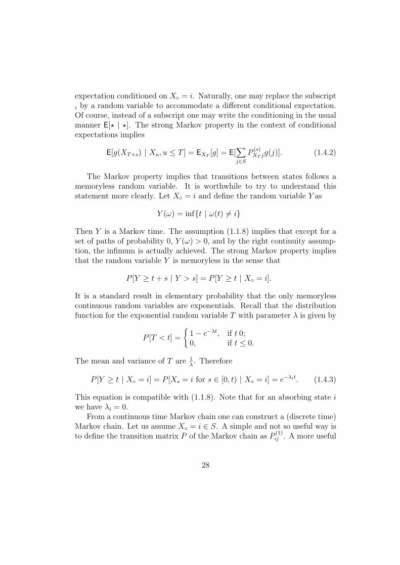
The Markov property implies that transitions between states follows amemoryless random variable. It is worthwhile to try to understand thisstatement more clearly. Let X = i and define the random variable Y as

Y (ω) = inft | ω(t) 6= i

Then Y is a Markov time. The assumption (1.1.8) implies that except for aset of paths of probability 0, Y (ω) > 0, and by the right continuity assump-tion, the infimum is actually achieved. The strong Markov property impliesthat the random variable Y is memoryless in the sense that

P [Y ≥ t+ s | Y > s] = P [Y ≥ t | X = i].

It is a standard result in elementary probability that the only memorylesscontinuous random variables are exponentials. Recall that the distributionfunction for the exponential random variable T with parameter λ is given by

P [T < t] =

1− e−λt, if t 0;0, if t ≤ 0.

The mean and variance of T are 1λ. Therefore

P [Y ≥ t | X = i] = P [Xs = i for s ∈ [0, t) | X = i] = e−λit. (1.4.3)

This equation is compatible with (1.1.8). Note that for an absorbing state iwe have λi = 0.

From a continuous time Markov chain one can construct a (discrete time)Markov chain. Let us assume X = i ∈ S. A simple and not so useful way isto define the transition matrix P of the Markov chain as P

(1)ij . A more useful

28

approach is to let Tn be the time of the nth transition. Thus T1(ω) = s > 0means that there is j ∈ S, j 6= i, such that

ω(t) =i for t < s;j for s = t.

T1 is a stopping time if we assume that i is not an absorbing state. We defineQij to be the probability of the set of paths that at time 0 are in state i andat the time of the first transition they move to state j. Therefore

Qkk = 0, and∑j 6=i

Qij = 1.

Let Wn = Tn+1 − Tn denote the time elapsed between the nth and (n + 1)st

transitions. We define a Markov chain Z = X, Z2, · · · by setting Zn =XTn . Note that the strong Markov property for Xt is used in ensuring thatZ, Z1, Z2, · · · is a Markov chain since transitions occur at different times ondifferent paths. The following lemma clarifies the transition matrix of theMarkov chain Zn and sheds light on the transition matrices Pt.

Lemma 1.4.1 For a non-absorbing state k we have

P [Zn+1 = j,Wn > u | Z = i, Z1, · · · , Zn = k, T1, · · · , Tn] = Qkje−λku.

Furthermore Qkk = 0, Qkj ≥ 0 and∑j Qkj = 1, so that Q = (Qkj) is the

transition matrix for the Markov chain Zn. For an absorbing state k, λk = 0and Qkj = δkj.

Proof - Clearly the left hand side of the equation can be written in the form

P [XTn+Wn = j,Wn > u | XTn = k,Xt, t ≤ T ].

By the strong Markov property2 we can rewrite this as

P [XTn+Wn = j,Wn > u | XTn = k,Xt, t ≤ T ] = P [XW = j,W > u | X = k].

Right hand side of the above equation can be written as

P [XW = j | W > u,X = k]P [W > u | X = k].

2We are using a slightly more general version than the statement (1.4.1), but its validityis equally clear.

29

We haveP [XW = j | W > u,X = k] = P [XW = j | Xs = k for s ≤ u]

= P [Xu+W = j | Xu = k]= P [XW = j | X = k].

The quantity P [XW = j | X = k] is independent of u and we denote it byQkj. Combining this with (1.4.3) (exponential character of elapsed time Wn

between consecutive transitions) we obtain the desired formula. The validityof stated properties of Qkj is immediate. ♣

A immediate corollary of lemma 1.4.1 is that it allows to fill in the gapin the proof of lemma 1.1.3.

Corollary 1.4.1 Let i 6= j ∈ S, then either P(t)ij > 0 for all t > 0 or it

vanishes identically.

Proof - If P(t)ij > 0 for some t, then Qij > 0, and it follows that for all t > 0

P(t)ij > 0. ♣

This process of assigning a Markov chain to a continuous time Markovchain can be reversed to obtain (infinitely many) continuous time Markovchains from a discrete time one. In fact, for every j ∈ S let λj > 0 bea positive real number. Now given a Markov chain Zn with state space Sand transition matrix Q, let Wj be an exponential random variable withparameter λj. If j is not an absorbing state, then the first transition out of jhappens at time s > t with probability e−λjt and once the transition occursthe probability of hitting state k is

Qjk∑i6=j Qji

.

Lemma 1.4.1 does not give direct and adequate information about thebehavior of transition probabilities. However, combining it with the strongMarkov property yields an important integral equation satisfied by the tran-sition probabilities.

Lemma 1.4.2 Assume Xt has no absorbing states. For i, j ∈ S, the transi-tion probabilities P

(t)ij satisfy

P(t)ij = e−λitδij + λi

∫ t

e−λis

∑k

QikP(t−s)kj ds

30

Proof - We may assume i is not an absorbing state. Let T1 be the time offirst transition. Then trivially

P(t)ij = P [Xt = j, T1 > t | X = i] + P [Xt = j, T1 ≤ t | X = i].

The term containing T1 > t can be written as

P [Xt = j, T1 > t | X = i] = δijP [T1 > t | X = i] = e−λitδij.

By the strong Markov property the second term becomes

P [Xt = j, T1 ≤ t | X = i] =∫ t

P [T1 = s < t | X = i]P

(t−s)Xsj ds.

To make a substitution for P [T1 = s < t | X = i] from lemma 1.4.1 we haveto differentiate3 the the expression 1−Qike

−λis with respect to s. We obtain

P [Xt = j, T1 ≤ t | X = i] = λi

∫ t

∑k

e−λisQikP(t−s)kj ds,

from which the required result follows. ♣An application of this lemma will be given in the next subsection. Inte-

gral equations of the general form given in lemma 1.4.2 occur frequently inprobability. Such equations generally result from conditioning on a Markovtime together with the strong Markov property.

A consequence of lemma 1.4.2 is an explicit expression for the infinitesimalgenerator of a continuous time Markov chain.

Corollary 1.4.2 With the notation of lemma 1.4.2, the infinitesimal gener-ator of the continuous time Markov chain Xt is

Aij =−λi, if i = j;λiQij, if i 6= j.

Proof - Making the change of variable s = t − u in the integral in lemma1.4.2 we obtain

P(t)ij = e−λitδij + λi

∫ t

e−λiu

∑k

QikP(u)kj du.

3This is like the connection between the density function and distribution function ofa random variable.

31

Differentiating with respect to t yields

dP(t)ij

dt= −λie−λitδij + λie

−λit∑k

QikP(t)kj .

Taking limt→0+ we obtain the desired result. ♣

1.5 Brownian Motion

Brownian motion is the most basic example of a Markov process with con-tinuous state space and continuous time. In order to motivate some of thedevelpments it may be useful to give an intuitive description of Brownianmotion based on random walks on Z. In this subsection we give an intuitiveapproach to Brownian motion and show how certain quantities of interest canbe practically calculated. In particular, we give heuristic but not frivolousarguments for extending some of the properties of random walks and Markovchains to Brownian motion.

Recall that if X1, X2, · · · is a sequence of iid random variables with valuesin Z, then S = 0, S1 = X1, · · ·, and Sn = Sn−1 + Xn, · · ·, is the generalrandom walk on Z. Let us assume that E[Xi] = 0 and Var[Xi] = σ2 < ∞,or even that Xi takes only finitely many values. The final result whichis obtained by a limiting process will be practically independent of whichrandom walk, subject to the stated conditions on mean and variance, westart with, and in particular we may even start with the simple symmetricrandom walk. For t > 0 a real number define

Z(n)t =

1√nS[nt],

where [x] denotes the largest integer not exceeding x. It is clear that

E[Z(n)t ] = 0, Var[Z

(n)t ] =

[nt]σ2

n' tσ2, (1.5.1)

where the approximation ' is valid for large n. The interesting point is thatwith re-scaling by 1√

n, the variance becomes approximately independent of

n for large n. To make reasonable paths out of those for the random walkon Z in the limit of large n, we further rescale the paths of the random walkSnt in the time direction by 1

n. This means that if we fix a positive integer n

32

and take for instance t = 1, then a path ω between 0 and n will be squeezedin the horizontal (time) direction to the interval [0, 1] and the values will bemultiplied by 1√

n. The resulting path will still consist of broken line segments

where the points of nonlinearity (or non-differentiability) occur at kn, k =

1, 2, 3, · · ·. At any rate since all the paths are continuous, we may surmisethat the path space for limn→∞ is the space Ω = Cx [0,∞) of continuousfunction on [0,∞) and we may require ω(0) = x, some fixed number. Sincein the simple symmetric random walk, a path is just as likely to up as down weexpect, the same is true of the paths in the Brownian motion. A differentiablepath on the other hand has a definite preference at each point, namely,the direction of the tangent. Therefore it is reasonable to expect that withprobability 1 the paths in Brownian are nowhere differentiable in spite of thefact that we have not yet said anything about how probabilities should beassigned to the appropriate subsets of Ω. The assignment of probabilities isthe key issue in defining Brownian motion.

Let 0 < t1 < t2 < · · · < tm and we want to see what we can say aboutthe joint distribution of (Z

(n)t1 , Z

(n)t2 −Z(n)

t1 , · · · , Z(n)tm −Z(n)

tm−1). Note that these

random variables are independent while Z(n)t1 , Z

(n)t2 , · · · are not. By the central

limit theorem, for n sufficiently large,

Z(n)tk − Z

(n)tk−1

=1√n

(S[ntk] − S[tnk−1]

)is approximately normal with mean 0 and variance (tk− tk−1)σ

2. We assume

that taking the limit of n→∞ the process Z(n)t tends to a limit. Of course

this requires specifying the sense in which convergence takes place and proof,but because of the applicability of the central limit theorem we assign prob-abilities to sets of paths accordingly without going through a convergenceargument. More precisely, to the set of paths, starting at 0 at time 0, whichare in the open subset B ⊂ R at time t, it is natural to assign the probability

P [Zt ∈ B] =1√

2πtσ

∫Be−

u2

2tσ2 du. (1.5.2)

In view of independence of Zt1 and Zt2−Zt1 , the probability that Zt1 ∈ (a1, b1)and Zt2 − Zt1 ∈ (a2, b2), is

1

2πσ2√t1(t2 − t1)

∫ b1

a1

∫ b2

a2

e−

u21

2σ2t1 e−

u22

2σ2(t2−t1)du1du2.

33

Note that we are evaluating the probability of the event [Zt1 ∈ (a1, b1), Zt2−Zt1 ∈ (a2, b2)] and not [Zt1 ∈ (a1, b1), Zt2 ∈ (a2, b2)] since the random vari-ables Zt1 and Zt2 are not independent. This formula extends to probabilityof any finite number of increments. In fact, for 0 < t1 < t2 < · · · < tk thejoint density function for (Zt1 , Zt2 − Zt1 , · · · , Ztk − Ztk−1

) is the product

e−

u21

2σ2t1 e−

u22

2σ2(t2−t1) · · · e−

u2k

2σ2(tk−tk−1)

σk√

(2π)kt1(t2 − t1) · · · (tk − tk−1)

One refers to the property of independence of (Zt1 , Zt2−Zt1 , · · · , Ztk−Ztk−1)

as independence of increments. For future reference and economy of notationwe introduce

pt(x;σ) =1√

2πtσe−

x2

2tσ2 . (1.5.3)

For σ = 1 we simply write pt(x) for pt(x;σ).For both discrete and continuous time Markov chains the transition prob-

abilities were give by matrices Pt. Here the transition probabilities are en-coded in the Gaussian density function pt(x;σ). It is easier to introduce theanalogue of Pt for Brownian motion if we look at the dual picture where theaction of the semi-group Pt on functions on the state space is described. Justas in the case of continuous time Markov chains we set

(Ptψ)(x) = E[ψ(Zt) | Z = x] =∫ ∞

−∞ψ(y)pt(x− y;σ)dy, (1.5.4)

which is completely analogous to (??). The operators Pt (acting on whateverthe appropriate function space is) still have the semi-group property Ps+t =PsPt. In view of (1.5.4) the semi-group is equivalent to the statement∫ ∞

−∞ps(y − z;σ)pt(x− y;σ)dy = pt(x− z;σ). (1.5.5)

Perhaps the simplest way to see the validity of (1.5.5) is by making use ofFourier analysis which transforms convolutions into products as explainedearlier in subsection (XXXX). It is a straightforward calculation that

∫ ∞

−∞e−iλx

e−x2

2tσ2

√2πtσ

dx =1

πe−

λ2σ2t2 . (1.5.6)

34

From (??) and (1.5.6), the desired relation (1.5.5) and the semi-group prop-erty follow. An important feature of continuous time Markov chains is thatPt satisfied the the Kolmogorov forward and backward equations. In view ofthe semi-group property the same is true for Brownian motion and we willexplain in example 1.5.2 below what the infinitesimal generator of Brownianmotion is. With some of the fundamental definitions of Brownian motion inplace we now calculate some quantities of interest.

Example 1.5.1 Since the random variables Zs and Zt are dependent, it isreasonable to calculate their covaraince. Assume s < t, then we have

Cov(Zs, Zt) = Cov(Zs, Zt − Zs + Zs)(By independence of increments) = Cov(Zs, Zs)

= sσ2.This may appear counter-intuitive at first sight since one expects Zs and Ztto become more independent as t− s increases while the covariance depends

only on min(s, t) = s. However, if we divide Cov(Zs, Zt) by√

Var[Zs]Var[Zt]we see that the correlation tends to 0 as t increases for fixed s. ♠

Example 1.5.2 One of the essential features of continuous time Markovchains was the existence of the infinitesimal generator. In this example wederive a formula for the infinitesimal generator of Brownian motion. For afunction ψ on the state space R, the action of the semi-group Pt is given by(1.5.4). We set uψ(t, x) = u(t, x) = Ptψ. The Gaussian pt(x;σ) has variancetσ2 and therefore it tends to the δ-function supported at the origin as t→ 0,i.e.,

limt→0

(Ptψ)(x) = limt→0

u(t, x) = ψ(x).

It is straightforward to verify that

∂u

∂t=σ2

2

∂2u

∂x2. (1.5.7)

Therefore from the validity of Kolomogorov’s backward equation (dPt

dt= APt)

we conclude that the infinitesimal generator of Brownian motion is given by

A =σ2

2

d2

dx2. (1.5.8)

Thus the matrix A is now replaced by a differential operator. ♠

35

Example 1.5.3 The notion of hitting time of a state played an importantrole in our discussion of Markov chains. In this example we calculate thedensity function for hitting time of a state a ∈ R in Brownian motion. Thetrick is to look at the identity

P [Zt > a] = P [Zt > a | Ta ≤ t]P [Ta ≤ t] + P [Zt > a | Ta > t]P [Ta > t].

Clearly the second term on the right hand side vanishes, and by symmetry

P [Zt > a | Ta < t] =1

2.

ThereforeP [Ta < t] = 2P [Zt > a]. (1.5.9)

The right hand side is easily computable and we obtain

P [Ta < t] =2√

2πtσ

∫ ∞

ae−

x2

2tσ2 dx =2√2π

∫ ∞

a√tσ

e−u2

2 du.

The density function for Ta is obtained by differentiating this expression withrespect to t:

fTa(t) =a√2πσ

1

t√te−

a2

2tσ2 . (1.5.10)

Since tfTa(t) ∼ c 1√t

as t→∞ for a non-zero constant c, we obtain

E[Ta] = ∞, (1.5.11)

which is similar to the case of simple symmetric random walk on Z. ♠

The reflection principle which we introduced in connection with the simplesymmetric random walk on Z and used to prove the arc-sine law is alsovalid for Brownian motion. However we have already accumulated enoughinformation to prove the arc-sine law for Brownian motion without referenceto the reflection principle. This is the substance of the following example:

Example 1.5.4 For Brownian motion with Z = 0 the event that it crossesthe line −a, where a > 0, between times 0 and t is identical with the event[T−a < t] and by symmetry it has the same probability as P [Ta < t]. Wecalculated this latter quantity in example 1.5.3. Therefore the probablity P

36

that the Brownian motion has at least one 0 in the interval (t1, t2) can bewritten as

P =1√

2πtσ

∫ ∞

−∞P [Ta < t1 − t]e

− a2

2tσ2 da. (1.5.12)

Let us explain the validity of this assertion. At time t, Zt can be at any

point a ∈ R. The Gaussian exponential factor 1√2πtσ

e− a2

2tσ2 is the density

function for Zt . The factor P [Ta < t1 − t] is equal to the probabilitythat starting at a, the Brownian motion will assume value 0 in the ensuingtime interval (t1 − t). The validity of the assertion follows from these factsput together. In view of the symmetry between a and −a, and the densityfunction for Ta which we obtained in example 1.5.3, (1.5.12) becomes

P = 2√2πtσ

∫∞ e−

a2

2tσ a√2πσ

(∫ t1−t e−

a2

2u1

u√udu)da

= 1πσ2

√t

∫ t1−t u−

32 (∫∞ ae−

a2

2σ2 ( 1u+ 1

t)da)du

=√tπ

∫ t1−t

du(u+t)

√u

The substitution√u = x yields

P =2

πtan−1

√t1 − tt

=2

πcos−1

√t1t, (1.5.13)

for the probability of at least one crossing of 0 betwen times t and t1. Itfollows that the probability of no crossing in the time interval (t, t1) is

2

πsin−1

√t1t

which is the arc-sine law for Brownian motion. ♠

So far we have only considered Brownian motion in dimension one. Bylooking at m copies of independent Brownian motions Zt = (Zt;1, · · · , Zt;m)we obtain Brownian motion in Rm. While m-dimensional Brownian motionis defined in terms of coordinates, there is no preference for any direction inspace. To see this more clearly, let A = (Ajk) be an m×m orthogonal matrix.This means that AA′ = I where superscript ′ denotes the transposition ofthe matrix, and geometrically it means that the linear transformation Apreserves lengths and therefore necessarily angles too. Let

Yt;j =m∑k=1

AjkZt;k.

37

Since a sum independent Gaussian random variables is Gaussian, Yt;j’s arealso Gaussian. Furthermore,

Cov(Yt;j, Yt;k) =m∑l=1

AjlAkl = δjk

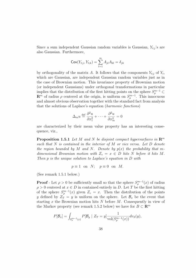
by orthogonality of the matrix A. It follows that the components Yt;j of Yt,which are Gaussian, are independent Gaussian random variables just as inthe case of Brownian motion. This invariance property of Brownian motion(or independent Gaussians) under orthogonal transformations in particularimplies that the distribution of the first hitting points on the sphere Sm−1

ρ ⊂Rm of radius ρ centered at the origin, is uniform on Sm−1

ρ . This innocuousand almost obvious observation together with the standard fact from analysisthat the solutions of Laplace’s equation (harmonic functions)

∆mudef=∂2u

∂x21

+ · · ·+ ∂2u

∂x2m

= 0

are characterized by their mean value property has an interesting conse-quence, viz.,

Proposition 1.5.1 Let M and N be disjoint compact hypersurfaces in Rm

such that N is contained in the interior of M or vice versa. Let D denotethe region bounded by M and N . Denote by p(x) the probability that m-dimensional Brownian motion with Z = x ∈ D hits N before it hits M .Then p is the unique solution to Laplace’s equation in D with

p ≡ 1 on N ; p ≡ 0 on M.

(See remark 1.5.1 below.)

Proof - Let ρ > 0 be sufficiently small so that the sphere Sm−1ρ (x) of radius

ρ > 0 centered at x ∈ D in contained entirely in D. Let T be the first hittingof the sphere Sm−1

ρ (x) given Z = x. Then the distribution of the pointsy defined by ZT = y is uniform on the sphere. Let Bx be the event thatstarting x the Brownian motion hits N before M . Consequently in view ofthe Markov property (see remark 1.5.2 below) we have for B ⊂ Rm

P [Bx] =∫Sm−1

ρ (x)P [By | ZT = y]

1

vol(Sm−1ρ (x))

dvS(y),

38

where dvS(y) denotes the standard volume element on the sphere Sm−1ρ (x).

Therefore we have

p(x) =∫Sm−1

ρ (x)

p(y)

vol(Sm−1ρ (x))

dvS(y), (1.5.14)

which is precisely the mean value property of harmonic functions. Theboundary conditions are clearly satisfied by p and the required result fol-lows. ♣

Remark 1.5.1 The condition that N is contained in the interior of M isintuitively clear in low dimensions and can be defined precisely in higherdimensions but it is not appropriate to dwell on this point in this context.This is not an essential assumption since the same conclusion remains valideven if D is an unbounded region by requiring the solution to Laplace’sequation to vanish at infinity. ♥

Remark 1.5.2 We are in fact using the strong Markov property of Brownianmotion. This application of this property is sufficiently intuitive that we didgive any further justification. ♥

Example 1.5.5 We specialize proposition 1.5.1 to dimensions 2 and 3 withN a sphere of radius ε > 0 and M a sphere of radius R, both centered atthe origin. In both cases we can obtain the desired solutions by writing theLaplacian ∆m in polar coordinates:

∆2 =1

r

∂

∂r(r∂

∂r) +

1

r2

∂2

∂θ2,

and

∆3 =1

r2

[∂

∂rr2 ∂

∂r+

1

sin θ

∂

∂θ(sin θ

∂

∂θ) +

1

sin2 θ

∂2

∂φ2

].

Looking for spherically symmetric solutions pm (i.e., depending only on thevariable r) the partial differential equations reduce to ordinary differentialequations which we easily solve to obtain the solutions

p2(x) =log r − logR

log ε− logR, for x = (r, θ), (1.5.15)

39

and

p3(x) =1r− 1

R1ε− 1

R

, for x = (r, θ, φ), (1.5.16)

for the given boundary conditions. Now notice that

limR→∞

p2(x) = 1, limR→∞

p3(x) =ε

r. (1.5.17)

The difference between the two cases is naturally interpreted as Brownianmotion being recurrent in dimension two but transient in dimensions ≥ 3. ♠

Remark 1.5.3 The functions u = 1rm−2 satisfies Laplace’s equation in Rm

for m ≥ 3, and can be used to rstablish the analogue of example 1.5.5 indimensions ≥ 4. ♥

Brownian motion has the special property that transition from a startingpoint x to a set A is determined by the integration of a function pt(x− y;σ)with respect to y on A. The fact that the integrand is a function of y − xreflects a space homogeneity property which Brownian shares with randomwalks. On the other hand, Markov chains do not in general enjoy such spacehomogeneity property. Naturally there are many pocesses that are Markovianin nature but do not have space homogeneity property. We present some suchexamples constructed from Brownian motion.

Example 1.5.6 Consider one dimensional Brownian motion with Z = x >0 and impose the condition that if for a path ω, ω(t) = 0, then ω(t) = 0 forall t > t. This is absorbed Brownian motion which we denote by Zt. Letus compute the transition probabilities for Zt. Unless stated to the contrary,in this example all probabilities and events involving Zt are conditioned onZ = x. For y > 0 let

Bt(y) = ω | ω(t) > y, min0≤s≤t

ω(s) > 0,

Ct(y) = ω | ω(t) > y, min0≤s≤t

ω(s) < 0.

We haveP [Zt > y] = P [Bt(y)] + P [Ct(y)]. (1.5.18)

By the reflection principle

P [Ct(y)] = P [Zt < −y].

40

ThereforeP [Bt(y)] = P [Zt > y]− P [Zt < −y]

= P [Zt > y − x | Z = 0]− P [Zt > x+ y | Z = 0]

= 1√2πtσ

∫ y+xy−x e

− u2

2tσ2 du

=∫ y+2xy pt(u− x;σ)du.

Therefore for Zt we haveP [Zt = 0 | Z = x] = 1− P [Bt(0)]

= 1−∫ x−x pt(u;σ)du

= 2∫∞ pt(x+ u;σ)du.

Similarly, for 0 < a < b,P [a < Zt < b] = P [Bt(a)]− P [Bt(b)]

=∫ ba [pt(u− x;σ)− pt(u+ x;σ)]du.

Thus we see that the transition probability has a discrete part P [Zt = 0 | Z =0] and a continuous part P [a < Zt < b] and is not a function of y − x. ♠

Example 1.5.7 Let Zt = (Zt;1, Zt;2) denote two dimensional Brownian mo-tion with Zt;i(0) = 0, and define

Rt =√Z2t;1 + Z2

t;2.

This process means that for every Brownian path ω we consider its dis-tance from the origin. This is a one dimensional process on R+, called radialBrownian motion or a Bessel process and its Markovian property is intuitivelyreasonable and will analytically follow from the calculation of transition prob-abilities presented below. Let us compute the transition probabilities. Wehave

P [Rt ≤ b] | Z = (x1, x2)] =∫ ∫

y+1 y22≤b2

12πtσ2 e

− (y1−x1)2+(y2−x2)2

2tσ2 dy1dy2

= 12πtσ2

∫ b∫ 2π e−

(r cos θ−x1)2+(r sin θ−x2)2

2tσ2 dθrdr

= r2πtσ2

∫ b e

− r2+ρ2

2tσ2 I(r, x)dr.where (r, θ) are polar coordinates in y1y2-plane, ρ = ||x|| and

I(r, x) =∫ 2π

e

rtσ2 [x1 cos θ+x2 sin θ]dθ.

Setting cosφ = x1

ρand sinφ = x2

ρ, we obtain

I(r, x) =∫ 2π

e

rρ

tσ2 cos θdθ.

41

The Bessel function I is defined as

I(α) =1

2π

∫ 2π

eα cos θdθ.

Therefore the desired transition probability

P [Rt ≤ b | Z = (x1, x2)] =∫ b

pt(ρ, r;σ)dr, (1.5.19)

where

pt(ρ, r;σ) =r

tσ2e−

r2+ρ2

2tσ2 I(rρ

tσ2).

The Markovian property of radial Brownian motion is a consequence of theexpression for transition probabilities since they depends only on (ρ, r). Fromthe fact that I is a solution of the differential equation

d2u

dz2+

1

z

du

dz− u = 0,

we obtain the partial differential differential equation satisfied p:

∂p

∂t=σ2

2

∂2p

∂r2+σ

2r

∂p

∂r,

which is the radial heat equation. ♠

The analogue of non-symmetric random walk (E[X] 6= 0) is Brownianmotion with drift µ which one may define as

Zµt = Zt + µt

in the one dimensional case. It is a simple exercise to show

Lemma 1.5.1 Zµt is normally distributed with mean µt and variance tσ2,

and has stationary independent increments.

In particular the lemma implies that, assuming Zµ = 0, the probability

of the set of paths that at time t are in the interval (a, b) is

1√2πtσ

∫ b

ae−

(u−µt)2

2tσ2 du.

42

Example 1.5.8 Let −b < 0 < a, x ∈ (−b, a) and p(x) be the probabilitythat Zµ

t hits a before it hits −b. This is similar to proposition 1.5.1. Insteadof using the mean value property of harmonic functions (which is no longervalid here) we directly use our knowledge of calculus to derive a differentialequation for p(x) which allows us to calculate it. The method of proof hasother applications (see exercise 1.5.5). Let h be a small number and B denotethe event that Zµ

t hits a before it hits −b. By conditioning on Zµh , and setting

Zµh = x+ y we obtain

p(x) =∫ ∞

−∞

1√2πhσ

e−(y−µh)2

2hσ2 p(x+ y)dy (1.5.20)

The Taylor expansion of p(x+ y) gives

p(x+ y) = p(x) + yp′(x) +1

2y2p′′(x) + · · ·

Now y = Zh − Z and therefore

∫ ∞

−∞ye−

(y−µh)2

2hσ2

√2πhσ

dy = µh,∫ ∞

−∞y2 e

− (y−µh)2

2hσ2

√2πhσ

dy = σ2h+ h2µ2.

It is straightforward to check that contribution of terms of the Taylor expan-sion containing yk, for k ≥ 3, is O(h2). Substituting in (1.5.20), dividing byh and taking limh→0 we obtain

σ2

2

d2p

dx2+ µ

dp

dx= 0.

The solution with the required boundary conditions is

p(x) =e

2µb

σ2 − e−2µx

σ2

e2µb

σ2 − e−2µa

σ2

.

The method of solution is applicable to other problems. ♠

43

EXERCISES

Exercise 1.5.1 Formulate the analogue of the reflection principle for Brow-nian motion and use it to give an alternative proof of (1.5.9).

Exercise 1.5.2 Discuss the analogue of example 1.5.5 in dimension 1.

Exercise 1.5.3 Generate ten paths for the simple symmetric random walkon Z for n ≤ 1000. Rescale the paths in time direction by 1

1000and in the

space direction by 1√1000

, and display them as graphs.

Exercise 1.5.4 Display ten paths for two dimensional Brownian motion byrepeating the computer simulation of exercise 1.5.3 for each component. Thepaths so generated are one dimensional curves in three dimensional space(time + space). Display only their projections on the space variables.

Exercise 1.5.5 Consider Brownian motion with drift Zµt and assume µ > 0.

Let −b < 0 < a and let T be the first hitting of the boundary of the interval[−b, a] and assume Zµ

= x ∈ (−b, a). Show that E[T ] < ∞. Derive adifferential equation for E[T ] and deduce that for σ = 1

E[T ] =a− x

µ+ (a+ b)

e−2µb − e−2µx

µ(e2µb − e−2µa).

Exercise 1.5.6 Consider Brownian motion with drift Zµt and assume µ > 0

and a > 0. Let T µa be the first hitting of the point a and

Ft(x) = P [T µx < t | Zµ = 0].

Using the method of example 1.5.8, derive a differential equation for Ft(x).

44