1

PH 240A: Chapter 12

Mark van der LaanUniversity of California Berkeley

(Slides by Nick Jewell)

2

Regression Models: Motivation

Stratification methods break down (wrt precision) with large number of strata and moderate sample sizes

Stratification leads to high degree of freedom tests for interaction, for example, and therefore low power

Refined measures of exposure lead to high degree of freedom tests for association and therefore low power

Want parsimonious descriptions of patterns of risk

Regression Models (how to diet wrt degrees of freedom)

3

Regression Models: Linking Effects

xx

x

x

X, numerical measure of Exposure E

P(D|E=x)

x1 x2 x4x3

4

Linear Models (think CHD and body weight)

Form of model:

Interpretation of model parameters a and b:

b = ER associated with unit increase in X b(x*-x) = ER assoc. with increase in X from x* to x

bxaxXDPpx +=== )|(

[ ] [ ]b

bxaxba

XxdpxXDPpp

aXDPp

xx

=

+−++=

=−+==−

===

+

)1(

)|()1|(

)0|(

1

0Choose X = 0 value carefully!

Choose the scale ofX carefully!

5

Linear Models

Pros Good modeling Excess Risk

Cons Can’t be applied to case-control data Can predict probabilities < 0 or > 1

6

Log Linear Models

Form of model:

Interpretation of model parameters a and b:

( ) ( )

bxax

x

ep

bxaxXDPp

+=

+=== )|(loglog

( ) ( )

( ) ( ) [ ] [ ]

bp

p

bxaxbapp

aXDPp

x

x

xx

=⎟⎟⎠

⎞⎜⎜⎝

⎛⇒

+−++=−

===

+

+

1

1

0

log

)1(loglog

)0|(loglog Choose X = 0 value carefully!

7

Log Linear Models

Interpretation of model parameters a and b:

eb = RR associated with unit increase in X

eb(x*-x) = RR assoc. with increase in X from x* to x

Choose the scale ofX carefully!

8

Log Linear Models

Pros Good modeling Relative Risk

Cons Can’t be applied to case-control data Can predict probabilities > 1

9

Logistic Regression Models

Form of model:

Interpretation of model parameters a and b:

( )

bxa

bxa

bxax

x

x

e

e

ep

bxaxXDp

p

+

+

+− +≡

+=

+===⎟⎟⎠

⎞⎜⎜⎝

⎛

−

11

1

|for oddslog1

log

)(

Choose X = 0 value carefully!

10

Logistic Regression Models

Interpretation of model parameters a and b:

eb = OR associated with unit increase in X

eb(x*-x) = OR assoc. with increase in X from x* to x

Choose the scale ofX carefully!

11

Logistic Regression Models

Pros Good modeling Odds Ratio Can be applied to case-control data Predicted probabilities always lie between 0 and 1

Cons Harder to interpret

12

Logistic Regression Models

13

1991 US Infant Mortality

Mother’s Marital Status

Infant Mortality

Unmarried

(X = 1)

Married(X = 0)

Total

Death 16,712 18,784 35,496

Live at 1 Year

1,197,142

2,878,421

4,075,563

Total 1,213,854

2,897,205

4,111,059

)0073.00065.00138.0(

0073.00065.0 :ModelLinear

01 =−=−=+=

ppERxpx

)7531.0)0065.0/0138.0log(logloglog

0385.50065.0loglog(

7531.00385.5)log( :Modellinear -Log

01

0

==−==−===

+−=

ppbRRpa

xpx

p1 = 16,712/1,213,854 = 0.0138p0 = 18,784/2,897,205 = 0.0065

)7604.0)1/log()1/log(log

0320.5)9935.0/0065.0log()1/log((

7604.00320.5)1/log( :Model Logistic

0011

00

=−−−==−==−=

+−=−

ppppbORppa

xpp xx

14

Infant Mortality and Marital Status: Various Models

15

Logistic Regression: Body Weight and CHD

16

CHD and Body Weight: Various Models

17

Multiple Logistic Regression Models

Form of model:

( )

kk

kk

kkk

k

k

xbxbxba

xbxbxba

xbxbxbaxx

kk

kkxx

xx

e

e

ep

xbxbxba

xXxXDp

p

++++

++++

++++− +≡

+=

++++=

===⎟⎟⎠

⎞⎜⎜⎝

⎛

−

L

L

LK

K

K

L

K

2211

2211

22111

1

1

111

,,|for oddslog1

log

)(,,

2211

11,,

,,

Think, e.g., D = CHD, X1 = Behavior type, X2 = Body weight

18

Multiple Logistic Regression Models

Interpretation of model parameters a, b1, . . ., bk :

( ) ( )

[ ] [ ] 122112211

,,,,,,,,,1,,,1,,,,,,

,,,1,,,1

0,,0

0,,0

)1(

)1/(log)1/(log)1/(

)1/(log

1log

21212121

2121

2121

bxbxbxbaxbxbxba

pppppp

pp

ap

p

kkkk

xxxxxxxxxxxxxxxxxx

xxxxxx

kkkk

kk

kk

=++++−+++++=

−−−=⎟⎟⎠

⎞⎜⎜⎝

⎛

−

−

=⎟⎟⎠

⎞⎜⎜⎝

⎛

−

++++

LL

KKKKKK

KK

K

K Choose 0 covariatevalues carefully!

Choose covariate scales carefully!

19

Indicator (Dummy) Variables for Discrete Exposures

Goal: to model exposures with several discrete levels without assuming dose response Body weight (dose response)

Body weight (no assumed pattern)

bxap

pX

x

x +=⎟⎟⎠

⎞⎜⎜⎝

⎛

−

⎪⎪⎪

⎩

⎪⎪⎪

⎨

⎧

>≤<≤<≤<

≤

=1

log

lbs 180 wt4lbs180wt1703lbs170wt1602lbs160wt1501

lbs150wt0

⎩⎨⎧ >

=⎩⎨⎧ ≤<

=

⎩⎨⎧ ≤<

=⎩⎨⎧ ≤<

=

otherwise0

lbs180wt1

otherwise0

lbs180wt1701

otherwise0

lbs170wt1601

otherwise0

lbs160wt1501

43

21

XX

XX

44332211,,

,,

41

41

1log xbxbxbxba

p

p

xx

xx ++++=⎟⎟⎠

⎞⎜⎜⎝

⎛

− K

K

20

Indicator (Dummy) Variables for Discrete Exposures

Model:44332211

,,

,,

41

41

1log xbxbxbxba

p

p

xx

xx ++++=⎟⎟⎠

⎞⎜⎜⎝

⎛

− K

K

lbs 180 wt

lbs180wt170

lbs170wt160

lbs160wt150

lbs150wt

odds log

4

3

2

1

⎪⎪⎪

⎩

⎪⎪⎪

⎨

⎧

>+≤<+≤<+≤<+

≤

=

babababa

a

No assumed pattern!

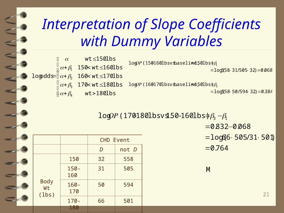
21

Interpretation of Slope Coefficients with Dummy

Variables

lbs 180 wt

lbs180wt170

lbs170wt160

lbs160wt150

lbs150wt

odds log

4

3

2

1

⎪⎪⎪

⎩

⎪⎪⎪

⎨

⎧

>+≤<+≤<+≤<+

≤

=

babababa

a

384.0)32594/50558log(

lbs) 150 baseline, vs.lbs 170-(160 log

068.0)32505/31558log(

lbs) 150 baseline, vs.lbs 160-(150 log

2

1

=××==<

=××==<

bOR

bOR

M

764.0

)50131/50566log(

068.0832.0

lbs) 160- 150 vs.lbs 180-(170 log 13

=××=

−=−= bbOR

CHD Event

D not D

Body Wt

(lbs)

150 32 558

150-160

31 505

160-170

50 594

170-180

66 501

>180 78 739

22

Indicator (Dummy) Variables for Discrete Exposures

Model Parameter Estimate OR

a -2.839

b 0.180 1.20

a -2.859

b1 0.068 1.07

b2 0.384 1.47

b3 0.832 2.30

b4 0.610 1.84

bxap

p

x

x +=⎟⎟⎠

⎞⎜⎜⎝

⎛

−1log

4433

2211,,

,,

1log

41

41

xbxb

xbxbap

p

xx

xx

++

++=⎟⎟⎠

⎞⎜⎜⎝

⎛

− K

K

23

Logistic Regression: Body Weight and CHD

Dose response (linear) X

No pattern (dummy vars.) X1, . . . , X4