Embed Size (px)
Citation preview
16920JSMA 5212 Numerical Methods for PDEs
Lecture 5
Finite Differences Parabolic Problems
B C Khoo
Thanks to Franklin Tan
SMA-HPC copy2002 NUS
SMA-HPC copy2002 NUS 2
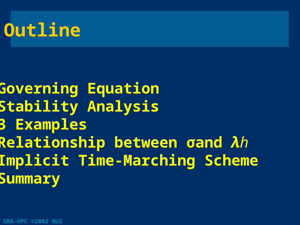
Outline
bull Governing Equation bull Stability Analysis bull 3 Examples bull Relationship between σand λh bull Implicit Time-Marching Scheme bull Summary
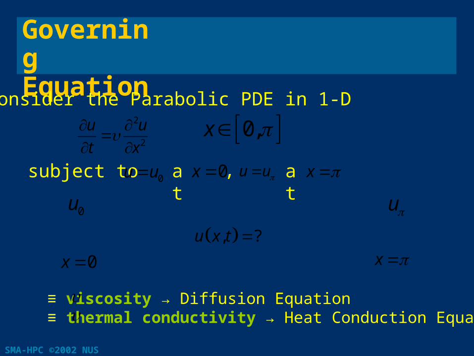
GoverningEquation
Consider the Parabolic PDE in 1-D
subject to
bull If equiv viscosity rarr Diffusion Equation bull If equiv thermal conductivity rarr Heat Conduction Equation
2
2
u u
t x
0x
0u u 0x u u x
u x t
at at
0u u
0x x
SMA-HPC copy2002 NUS 3
SMA-HPC copy2002 NUS 4
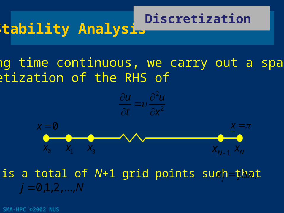
Stability Analysis Discretization
Keeping time continuous we carry out a spatial discretization of the RHS of
2
2
u u
t x
There is a total of N+1 grid points such that 012j N
jx j x
0x x
0x 1x 3x1Nx Nx
SMA-HPC copy2002 NUS 5
Stability Analysis Discretization
Use the Central Difference Scheme for 2
2
u
x
2
2
j
u
x
1 12i j ju u u 2x
2O x
which is second-order accurate
bull Schemes of other orders of accuracy may be constructed
SMA-HPC copy2002 NUS 6
Stability Analysis Discretization
We obtain at 11 1 22 20
dux u u u
dt x
22 1 2 32
2du
x u u udt x
1 12 2j
j j j j
dux u u u
dt x
11 2 12 2N
N N N N
dux u u u
dt x
Note that we need not evaluate
are given as boundary conditions
at and
since and
u 0x x Nx x
0u Nu
SMA-HPC copy2002 NUS 7
Stability Analysis Matrix Formulation
Assembling the system of equations we obtain
1
2
2
1
j
N
du
dtdu
dt
du x
dt
du
dt
2 1
1 2 1
1 2 1
1
1 2
0
0
A
1
2
1
j
N
u
u
u
u
02
2
0
0
0
N
u
x
u
x
SMA-HPC copy2002 NUS 8
Stability Analysis PDE to Coupled ODEs
Or in compact form
We have reduced the 1-D PDE to a set of Coupled ODEs
duAu b
dt
where 1
02 2
0 0 0
T
2 N -1
T
N
u u u u
u ub
x x
SMA-HPC copy2002 NUS 9
Stability Analysis Eigenvalue and
Eigenvector of Matrix A
If A is a nonsingular matrix as in this case it is then possible to find a set of eigenvalues
from det 0A I
1 2 1 j N
For each eigenvalue we can evaluate the eigenvector consisting of a set of mesh point values ie
jjV
ji
j j1 2 N-1 jT jV
SMA-HPC copy2002 NUS 10
Stability Analysis Eigenvalue and
Eigenvector of Matrix A
The (N-1) times (N- 1) matrix E formed by the (N-1) columns Vjdiagonalizes the matrix A by
1E AE
where
1
2
1N
0
0
SMA-HPC copy2002 NUS 11
Stability Analysis Coupled ODEs toUncoupled ODEs
Starting from
Premultiplication by yields
duAu b
dt
1E
1 1 1
1 1 1 1
1 1 1 1
I
duE E Au E b
dtdu
E E A EE u E bdt
duE E AE E u E b
dt
SMA-HPC copy2002 NUS 12
Stability Analysis Coupled ODEs toUncoupled ODEs
Continuing from
Let and we have
which is a set of Uncoupled ODEs
dU U F
dt
1F E b
1U E u
1 1 1duE E u E b
dt
SMA-HPC copy2002 NUS 13
Stability Analysis Coupled ODEs toUncoupled ODEs
Expanding yields
Since the equations are independent of one another they can be solved separately
The idea then is to solve for and determine
11 1 1
22 2 2
11 1 1
jj j j
NN N N
dUU F
dtdU
U Fdt
dUU F
dt
dUU F
dt
U
u EU
SMA-HPC copy2002 NUS 14
Stability Analysis Coupled ODEs toUncoupled ODEs
Considering the case of independent of time for the general equation
is the solution for
Evaluating
Complementary (transient) solution
Particular (steady-state) solution
where
b
thj 1jtj j j
j
U c e F
12 1j N
1 1tu EU E ce E E b
11 21 2 1 j N
Tt tt ttj Nce c e c e c e c e
SMA-HPC copy2002 NUS 15
Stability Analysis Stability Criterion
We can think of the solution to the semi-discretized problem
as a superposition of eigenmodes of the matrix operator A
Each mode contributes a (transient) time behaviour of the form to the time-dependent part of the solution
Since the transient solution must decay with time
This is the criterion for stability of the space discretization (of a parabolic PDE) keeping time continuous
for all
jjte
j
1 1tu E ce E E b
jReal 0
SMA-HPC copy2002 NUS 16
Stability Analysis Use of Modal (Scalar)
Equation
It may be noted that since the solution is expressed as a contribution from all the modes of the initial solution which have propagated or (and) diffused with the eigenvalue and a contribution from the source term all the properties of the time integration (and their stability properties) can be analysed separately for each mode with the scalar equation
j
dUU F
dt
u
j jb
SMA-HPC copy2002 NUS 17
Stability Analysis Use of Modal (Scalar)
Equation
The spatial operator A is replaced by an eigenvalue λ and the above modal equation will serve as the basic equation for analysis of the stability of a time-integration scheme (yet to be introduced) as a function of the eigenvalues λof the space-discretization operators
This analysis provides a general technique for the determination of time integration methods which lead to stable algorithms for a given space discretization
SMA-HPC copy2002 NUS 18
Example 1 Continuous Time
Operator
Consider a set of coupled ODEs (2 equations only)
111 1 12 2
221 1 22 2
dua u a u
dtdu
a u a udt
1 11 12
2 21 22
Let u u a a du
A Auu a a dt
SMA-HPC copy2002 NUS 19
Example 1 Continuous Time
Operator
Proceeding as before or otherwise (solving the ODEs directly) we can obtain the solution
1 2
1 2
1 1 11 2 12
2 1 21 2 22
t t
t t
u c e c e
u c e c e
Where and are eigenvalues of A and and are
eigenvectors pertaining to and respectively
As the transient solution must decay with time it is imperative that
11
21
21
22
Real 0 for 1 2j j
1 2
1 2
SMA-HPC copy2002 NUS 20
Example 1 Discrete Time Operator
Suppose we have somehow discretized the time operator on the LHS to obtain
where the superscript n stands for the nth time level then
Since A is independent of time
1 11 11 1 12 2
1 12 21 1 22 2
n n n
n n n
u a u a u
u a u a u
Where and 1n nu Au
1 2
Tn n nu u u 11 12
21 22
a aA
a a
1 2 0n n n nu Au AAu A u
SMA-HPC copy2002 NUS 21
Example 1 Discrete Time Operator
As 1
1 1 1 0
1 0
n
n n
A A A
A E E
u E E E E E E u
u E E u
where 1
2
0
0
nn
n
1 1 11 1 2 12 2
2 1 21 1 2 22 2
n n n
n n n
u c c
u c c
1 1 0
2
cE u
c
Where are constants
SMA-HPC copy2002 NUS 22
Example 1 Comparison
Comparing the solution of the semi-discretized problem where time is kept continuous
to the solution where time is discretized
The difference equation where time is continuous has exponential solution The difference equation where time is discretized has power solution
1
2
1 11 121 2
2 21 22
t
t
u ec c
u e
1 11 12 11 2
2 21 22 2
n n
n
uc c
u
te
n
SMA-HPC copy2002 NUS 23
Example 1 Comparison
In equivalence the transient solution of the difference equation must decay with time ie
for this particular form of time discretization
1n
SMA-HPC copy2002 NUS 24
Example 2
Consider a typical modal equation of the form
where is the eigenvalue of the associated matrix A
(For simplicity we shall henceforth drop the subscript j) We shall apply the ldquoleapfrogrdquo time discretization scheme given as
Substituting into the modal equation yields
1 1
= +2
= +
n nt
t nh
n hn
u uu ae
h
u ae
t
j
duu ae
dt
j
1 1
2
n ndu u uh t
dt h
where
Leapfrog Time Discretization
SMA-HPC copy2002 NUS 25
Example 2 Leapfrog Time Discretization
Time Shift Operator
1 1
1 1 2 22
n nn hn n n n hnu u
u ae u h u u ha eh
Solution of u consists of the complementary solution cn and the particular solution pn ie
n n nu c p There are several ways of solving for the complementary and particular solutions One way is through use of the shift operator S and characteristic polynomial The time shift operator S operates on cn such that
1
2 1 2
n n
n n n n
Sc c
S c S Sc Sc c
SMA-HPC copy2002 NUS 26
Example 2 Leapfrog Time Discretization
Time Shift Operator
The complementary solution cn satisfies the homogenous equation
1 1
2
2
2 0
2 0
12 0
2 1 0
n n n
nn n
n n n
n
c h c c
cSc h c
S
S c h Sc cS
cS h S
S
characteristic polynomial
2 2 1 0p S S h S
SMA-HPC copy2002 NUS 27
Example 2 Leapfrog Time Discretization
Time Shift Operator
The solution to the characteristic polynomial is
The complementary solution to the modal equation would then be
The particular solution to the modal equation is
Combining the two components of the solution together
2 21h S h h
1 1 2 2n n nc
2
2
2 1
hn hn
h h
ahe ep
e h e
2 2 2 21 2
2 1 2 1
2 1
n n n
hn hn n
h h
u c p
ahe eh h h h
e h e
σ1 and σ2 are the two roots
SMA-HPC copy2002 NUS 28
Example 2 Leapfrog Time Discretization
Stability Criterion
For the solution to be stable the transient (complementary) solution must not be allowed to grow indefinitely with time thus implying that
is the stability criterion for the leapfrog time discretization scheme used above
2 21
2 22
1 1
1 1
h h
h h
SMA-HPC copy2002 NUS 29
Example 2 Leapfrog Time Discretization
Stability Diagram
The stability diagram for the leapfrog (or any general) time discretization scheme in the σ-plane is
Region of Stability
Im(σ)
Re(σ)
SMA-HPC copy2002 NUS 30
Example 2 Leapfrog Time Discretization
In particular by applying to the 1-D Parabolic PDE
the central difference scheme for spatial discretization weobtain
which is the tridiagonal matrix
2
2
u u
t x
2
2 1
1 2 1
1
1 2
0
0
Ax
SMA-HPC copy2002 NUS 31
Example 2 Leapfrog Time Discretization
According to analysis of a general triadiagonal matrix B(abc) the eigenvalues of the B are
The most ldquodangerousrdquo mode is that associated with the eigenvalue of largest magnitude
which can be plotted in the absolute stability diagram
2
2 cos 1 2 1
2 2cos
j
j
jb ac j N
N
j
N x
2
4MAX x
2 21
2 22
ie 1
1
MAX MAX MAX
MAX MAX MAX
h h h
h h h
SMA-HPC copy2002 NUS 32
Example 2 Leapfrog Time Discretization
Absolute Stability Diagram for σ
As applied to the 1-D Parabolic PDE the absolute stability diagram for σis
σ1with h increasing
Region of stability
σ2 at h = Δt = 0
Unit circle
σ1 at h = Δt = 0
Re(σ)
Im(σ)
Region of instability
σ2 with h increasing
SMA-HPC copy2002 NUS 33
Stability Analysis Some Important
Characteristics Deduced
A few features worth considering
1 Stability analysis of time discretization scheme can be carried out for all the different modes
2 If the stability criterion for the time discretization scheme is valid for all modes then the overall solution is stable (since it is a linear combination of all the modes)
3 When there is more than one root σ then one of them is the principal root which represents an approximation to the physical behaviour The principal root is recognized by the fact that it tends towards one as (The other roots are spurious which
affect the stability but not the accuracy of the scheme)
j
0
0 lim 1h
h i e h
SMA-HPC copy2002 NUS 34
Stability Analysis Some Important
Characteristics Deduced
4 By comparing the power series solution of the principal root to one can determine the order of accuracy of the time discretization scheme In this example of leapfrog time discretization
he
1
2 2 2 2 4 421
2 2
1
1 11 2 21 12 2
12
h h h h h
hh
2 2
12
h he h
and compared to
is identical up to the second order of Hence the above scheme is said to be second-order accurate
h
SMA-HPC copy2002 NUS 35
Example 3 Euler-Forward Time Discretization
Stability Analysis
Analyze the stability of the explicit Euler-forward time discretization
as applied to the modal equation
into the modal equation we obtain
Substituting where
du
dt
1n nu u t
duu
dt
1 n n duu u h h t
dt
1 1 0n nu h u
SMA-HPC copy2002 NUS 36
Example 3 Euler-Forward Time Discretization
Stability Analysis
Making use of the shift operator S
The Euler-forward time discretization scheme is stable if
characteristic polynomial
Therefore
and
or bounded by
1 1 1 1 0n n n n nc h c Sc h c S h c
1n n
h h
c
1 1h
1h 1 hst in the -plane
SMA-HPC copy2002 NUS 37
Example 3 Euler-Forward Time Discretization
Stability Diagram
The stability diagram for the Euler-forward time discretization in the -plane is h
Region of Stability
Unit Circle Im( ) h
Re( ) h
SMA-HPC copy2002 NUS 38
Example 3 Euler-Forward Time Discretization
Absolute Stability Diagram
As applied to the 1-D Parabolic PDE 2
4max x
Im(σ)
Re(σ)
at 0h t
σleaves the unit circle at λh = minus2
The stability limit for largest 2
max
h t
σwith h increasing
SMA-HPC copy2002 NUS 39
σ = σ(λh) Relationshipbetweenσandλh
Thus far we have obtained the stability criterion of the time discretization scheme using a typical modal equation We cangeneralize the relationship between σand λh as follows
bull Starting from the set of coupled ODEs
bull Apply a specific time discretization scheme like the ldquoleapfrogrdquo time discretization as in Example 2
duAu b
dt
1 1
2
n ndu u u
dt h
SMA-HPC copy2002 NUS 40
σ = σ(λh) Relationshipbetweenσandλh bull The above set of ODEs becomes
bull Introducing the time shift operator S
bull Premultiplying E-1on the LHS and RHS and introducing I=EE-1 operating on
11 1 1 1
2
nS SE AE E E E u E b
h
1 1
2
n nn nu u
Au bh
1
2 2
2
nn n n
n n
uSu hAu hb
S
S SA I u b
h
SMA-HPC copy2002 NUS 41
σ = σ(λh) Relationshipbetweenσandλh
bull Putting
we obtain
which is a set of uncoupled equations
Hence for each j j = 12hellipN-1
1 1 n n n nU E u F E b
11
1
2
2
n nS SE E U F
h
S S
h
1
ie 2
n nS SU F
h
1
2j j j
S SU F
h
SMA-HPC copy2002 NUS 42
σ = σ(λh) Relationshipbetweenσandλh Note that the analysis performed above is identical to the analysis carried out using the modal equation
All the analysis carried out earlier for a single modal equation is applicable to the matrix after the appropriate manipulation to obtain an uncoupled set of ODEs
Each equation can be solved independently for and the s can then be coupled through
j
dUU F
dt
thjnjU n nu EU
njU
SMA-HPC copy2002 NUS 43
σ = σ(λh) Relationshipbetweenσandλh
Hence applying any ldquoconsistentrdquo numerical technique to each equation in the set of coupled linear ODEs is mathematically equivalent to
1 Uncoupling the set
2 Integrating each equation in the uncoupled set
3 Re-coupling the results to form the final solution
These 3 steps are commonly referred to as the
ISOLATION THEOREM
SMA-HPC copy2002 NUS 44
Implicit Time-Marching Scheme
Thus far we have presented examples of explicit time-marching methods and these may be used to integrate weakly stiff equations
Implicit methods are usually employed to integrate very stiff ODEs efficiently However use of implicit schemes requires solution of a set of simultaneous algebraic equations at each time-step (ie matrix inversion) whilst updating the variables at the same time
Implicit schemes applied to ODEs that are inherently stable will be unconditionally stable or A-stable
SMA-HPC copy2002 NUS 45
Euler-Backward Implicit Time-Marching Scheme
Consider the Euler-backward scheme for time discretization
Applying the above to the modal equation for Parabolic PDE
yields
1 1n n ndu u u
dt h
tduu ae
dt
111
111
n nn hn
n hn n
u uu ae
h
h u u ahe
SMA-HPC copy2002 NUS 46
Euler-Backward Implicit Time-Marching Scheme
Applying the S operator
the characteristic polynomial becomes
The principal root is therefore
which upon comparison with is only first-order accurate
The solution is
11 1 n hnh S u ahe
P P 1 1 0S h S
2 211
1h h
h
2 211
2he h h
11
1 1 1
n u hn
h
aheU
h h e
SMA-HPC copy2002 NUS 47
Euler-Backward Implicit Time-Marching Scheme
For the Parabolic PDE λis always real and lt 0 Therefore the transient component will always tend towards zero for large n irregardless of h (equivΔt)
The time-marching scheme is always numerically stable
In this way the implicit EulerEuler-backward time discretization scheme will allow us to resolve different time-scaled events with the use of different time-step sizes A small time-step size is used for the short time-scaled events and then a large time-step size used for the longer time-scaled events There is no constraint on hmax
SMA-HPC copy2002 NUS 48
Euler-Backward Implicit Time-Marching Scheme
However numerical solution of u requires the solution of a set of simultaneous algebraic equations or matrix inversion which is computationally much more intensiveexpensive compared to the multiplication addition operations of explicit schemes
SMA-HPC copy2002 NUS 49
Summary
bull Stability Analysis of Parabolic PDE 1048707 Uncoupling the set 1048707 Integrating each equation in the uncoupled set rarr modal equation 1048707 Re-coupling the results to form final solution
bull Use of modal equation to analyze the stability |σ(λh)| lt 1
bull Explicit time discretization versus Implicit time discretization
SMA-HPC copy2002 NUS 2
Outline
bull Governing Equation bull Stability Analysis bull 3 Examples bull Relationship between σand λh bull Implicit Time-Marching Scheme bull Summary
GoverningEquation
Consider the Parabolic PDE in 1-D
subject to
bull If equiv viscosity rarr Diffusion Equation bull If equiv thermal conductivity rarr Heat Conduction Equation
2
2
u u
t x
0x
0u u 0x u u x
u x t
at at
0u u
0x x
SMA-HPC copy2002 NUS 3
SMA-HPC copy2002 NUS 4
Stability Analysis Discretization
Keeping time continuous we carry out a spatial discretization of the RHS of
2
2
u u
t x
There is a total of N+1 grid points such that 012j N
jx j x
0x x
0x 1x 3x1Nx Nx
SMA-HPC copy2002 NUS 5
Stability Analysis Discretization
Use the Central Difference Scheme for 2
2
u
x
2
2
j
u
x
1 12i j ju u u 2x
2O x
which is second-order accurate
bull Schemes of other orders of accuracy may be constructed
SMA-HPC copy2002 NUS 6
Stability Analysis Discretization
We obtain at 11 1 22 20
dux u u u
dt x
22 1 2 32
2du
x u u udt x
1 12 2j
j j j j
dux u u u
dt x
11 2 12 2N
N N N N
dux u u u
dt x
Note that we need not evaluate
are given as boundary conditions
at and
since and
u 0x x Nx x
0u Nu
SMA-HPC copy2002 NUS 7
Stability Analysis Matrix Formulation
Assembling the system of equations we obtain
1
2
2
1
j
N
du
dtdu
dt
du x
dt
du
dt
2 1
1 2 1
1 2 1
1
1 2
0
0
A
1
2
1
j
N
u
u
u
u
02
2
0
0
0
N
u
x
u
x
SMA-HPC copy2002 NUS 8
Stability Analysis PDE to Coupled ODEs
Or in compact form
We have reduced the 1-D PDE to a set of Coupled ODEs
duAu b
dt
where 1
02 2
0 0 0
T
2 N -1
T
N
u u u u
u ub
x x
SMA-HPC copy2002 NUS 9
Stability Analysis Eigenvalue and
Eigenvector of Matrix A
If A is a nonsingular matrix as in this case it is then possible to find a set of eigenvalues
from det 0A I
1 2 1 j N
For each eigenvalue we can evaluate the eigenvector consisting of a set of mesh point values ie
jjV
ji
j j1 2 N-1 jT jV
SMA-HPC copy2002 NUS 10
Stability Analysis Eigenvalue and
Eigenvector of Matrix A
The (N-1) times (N- 1) matrix E formed by the (N-1) columns Vjdiagonalizes the matrix A by
1E AE
where
1
2
1N
0
0
SMA-HPC copy2002 NUS 11
Stability Analysis Coupled ODEs toUncoupled ODEs
Starting from
Premultiplication by yields
duAu b
dt
1E
1 1 1
1 1 1 1
1 1 1 1
I
duE E Au E b
dtdu
E E A EE u E bdt
duE E AE E u E b
dt
SMA-HPC copy2002 NUS 12
Stability Analysis Coupled ODEs toUncoupled ODEs
Continuing from
Let and we have
which is a set of Uncoupled ODEs
dU U F
dt
1F E b
1U E u
1 1 1duE E u E b
dt
SMA-HPC copy2002 NUS 13
Stability Analysis Coupled ODEs toUncoupled ODEs
Expanding yields
Since the equations are independent of one another they can be solved separately
The idea then is to solve for and determine
11 1 1
22 2 2
11 1 1
jj j j
NN N N
dUU F
dtdU
U Fdt
dUU F
dt
dUU F
dt
U
u EU
SMA-HPC copy2002 NUS 14
Stability Analysis Coupled ODEs toUncoupled ODEs
Considering the case of independent of time for the general equation
is the solution for
Evaluating
Complementary (transient) solution
Particular (steady-state) solution
where
b
thj 1jtj j j
j
U c e F
12 1j N
1 1tu EU E ce E E b
11 21 2 1 j N
Tt tt ttj Nce c e c e c e c e
SMA-HPC copy2002 NUS 15
Stability Analysis Stability Criterion
We can think of the solution to the semi-discretized problem
as a superposition of eigenmodes of the matrix operator A
Each mode contributes a (transient) time behaviour of the form to the time-dependent part of the solution
Since the transient solution must decay with time
This is the criterion for stability of the space discretization (of a parabolic PDE) keeping time continuous
for all
jjte
j
1 1tu E ce E E b
jReal 0
SMA-HPC copy2002 NUS 16
Stability Analysis Use of Modal (Scalar)
Equation
It may be noted that since the solution is expressed as a contribution from all the modes of the initial solution which have propagated or (and) diffused with the eigenvalue and a contribution from the source term all the properties of the time integration (and their stability properties) can be analysed separately for each mode with the scalar equation
j
dUU F
dt
u
j jb
SMA-HPC copy2002 NUS 17
Stability Analysis Use of Modal (Scalar)
Equation
The spatial operator A is replaced by an eigenvalue λ and the above modal equation will serve as the basic equation for analysis of the stability of a time-integration scheme (yet to be introduced) as a function of the eigenvalues λof the space-discretization operators
This analysis provides a general technique for the determination of time integration methods which lead to stable algorithms for a given space discretization
SMA-HPC copy2002 NUS 18
Example 1 Continuous Time
Operator
Consider a set of coupled ODEs (2 equations only)
111 1 12 2
221 1 22 2
dua u a u
dtdu
a u a udt
1 11 12
2 21 22
Let u u a a du
A Auu a a dt
SMA-HPC copy2002 NUS 19
Example 1 Continuous Time
Operator
Proceeding as before or otherwise (solving the ODEs directly) we can obtain the solution
1 2
1 2
1 1 11 2 12
2 1 21 2 22
t t
t t
u c e c e
u c e c e
Where and are eigenvalues of A and and are
eigenvectors pertaining to and respectively
As the transient solution must decay with time it is imperative that
11
21
21
22
Real 0 for 1 2j j
1 2
1 2
SMA-HPC copy2002 NUS 20
Example 1 Discrete Time Operator
Suppose we have somehow discretized the time operator on the LHS to obtain
where the superscript n stands for the nth time level then
Since A is independent of time
1 11 11 1 12 2
1 12 21 1 22 2
n n n
n n n
u a u a u
u a u a u
Where and 1n nu Au
1 2
Tn n nu u u 11 12
21 22
a aA
a a
1 2 0n n n nu Au AAu A u
SMA-HPC copy2002 NUS 21
Example 1 Discrete Time Operator
As 1
1 1 1 0
1 0
n
n n
A A A
A E E
u E E E E E E u
u E E u
where 1
2
0
0
nn
n
1 1 11 1 2 12 2
2 1 21 1 2 22 2
n n n
n n n
u c c
u c c
1 1 0
2
cE u
c
Where are constants
SMA-HPC copy2002 NUS 22
Example 1 Comparison
Comparing the solution of the semi-discretized problem where time is kept continuous
to the solution where time is discretized
The difference equation where time is continuous has exponential solution The difference equation where time is discretized has power solution
1
2
1 11 121 2
2 21 22
t
t
u ec c
u e
1 11 12 11 2
2 21 22 2
n n
n
uc c
u
te
n
SMA-HPC copy2002 NUS 23
Example 1 Comparison
In equivalence the transient solution of the difference equation must decay with time ie
for this particular form of time discretization
1n
SMA-HPC copy2002 NUS 24
Example 2
Consider a typical modal equation of the form
where is the eigenvalue of the associated matrix A
(For simplicity we shall henceforth drop the subscript j) We shall apply the ldquoleapfrogrdquo time discretization scheme given as
Substituting into the modal equation yields
1 1
= +2
= +
n nt
t nh
n hn
u uu ae
h
u ae
t
j
duu ae
dt
j
1 1
2
n ndu u uh t
dt h
where
Leapfrog Time Discretization
SMA-HPC copy2002 NUS 25
Example 2 Leapfrog Time Discretization
Time Shift Operator
1 1
1 1 2 22
n nn hn n n n hnu u
u ae u h u u ha eh
Solution of u consists of the complementary solution cn and the particular solution pn ie
n n nu c p There are several ways of solving for the complementary and particular solutions One way is through use of the shift operator S and characteristic polynomial The time shift operator S operates on cn such that
1
2 1 2
n n
n n n n
Sc c
S c S Sc Sc c
SMA-HPC copy2002 NUS 26
Example 2 Leapfrog Time Discretization
Time Shift Operator
The complementary solution cn satisfies the homogenous equation
1 1
2
2
2 0
2 0
12 0
2 1 0
n n n
nn n
n n n
n
c h c c
cSc h c
S
S c h Sc cS
cS h S
S
characteristic polynomial
2 2 1 0p S S h S
SMA-HPC copy2002 NUS 27
Example 2 Leapfrog Time Discretization
Time Shift Operator
The solution to the characteristic polynomial is
The complementary solution to the modal equation would then be
The particular solution to the modal equation is
Combining the two components of the solution together
2 21h S h h
1 1 2 2n n nc
2
2
2 1
hn hn
h h
ahe ep
e h e
2 2 2 21 2
2 1 2 1
2 1
n n n
hn hn n
h h
u c p
ahe eh h h h
e h e
σ1 and σ2 are the two roots
SMA-HPC copy2002 NUS 28
Example 2 Leapfrog Time Discretization
Stability Criterion
For the solution to be stable the transient (complementary) solution must not be allowed to grow indefinitely with time thus implying that
is the stability criterion for the leapfrog time discretization scheme used above
2 21
2 22
1 1
1 1
h h
h h
SMA-HPC copy2002 NUS 29
Example 2 Leapfrog Time Discretization
Stability Diagram
The stability diagram for the leapfrog (or any general) time discretization scheme in the σ-plane is
Region of Stability
Im(σ)
Re(σ)
SMA-HPC copy2002 NUS 30
Example 2 Leapfrog Time Discretization
In particular by applying to the 1-D Parabolic PDE
the central difference scheme for spatial discretization weobtain
which is the tridiagonal matrix
2
2
u u
t x
2
2 1
1 2 1
1
1 2
0
0
Ax
SMA-HPC copy2002 NUS 31
Example 2 Leapfrog Time Discretization
According to analysis of a general triadiagonal matrix B(abc) the eigenvalues of the B are
The most ldquodangerousrdquo mode is that associated with the eigenvalue of largest magnitude
which can be plotted in the absolute stability diagram
2
2 cos 1 2 1
2 2cos
j
j
jb ac j N
N
j
N x
2
4MAX x
2 21
2 22
ie 1
1
MAX MAX MAX
MAX MAX MAX
h h h
h h h
SMA-HPC copy2002 NUS 32
Example 2 Leapfrog Time Discretization
Absolute Stability Diagram for σ
As applied to the 1-D Parabolic PDE the absolute stability diagram for σis
σ1with h increasing
Region of stability
σ2 at h = Δt = 0
Unit circle
σ1 at h = Δt = 0
Re(σ)
Im(σ)
Region of instability
σ2 with h increasing
SMA-HPC copy2002 NUS 33
Stability Analysis Some Important
Characteristics Deduced
A few features worth considering
1 Stability analysis of time discretization scheme can be carried out for all the different modes
2 If the stability criterion for the time discretization scheme is valid for all modes then the overall solution is stable (since it is a linear combination of all the modes)
3 When there is more than one root σ then one of them is the principal root which represents an approximation to the physical behaviour The principal root is recognized by the fact that it tends towards one as (The other roots are spurious which
affect the stability but not the accuracy of the scheme)
j
0
0 lim 1h
h i e h
SMA-HPC copy2002 NUS 34
Stability Analysis Some Important
Characteristics Deduced
4 By comparing the power series solution of the principal root to one can determine the order of accuracy of the time discretization scheme In this example of leapfrog time discretization
he
1
2 2 2 2 4 421
2 2
1
1 11 2 21 12 2
12
h h h h h
hh
2 2
12
h he h
and compared to
is identical up to the second order of Hence the above scheme is said to be second-order accurate
h
SMA-HPC copy2002 NUS 35
Example 3 Euler-Forward Time Discretization
Stability Analysis
Analyze the stability of the explicit Euler-forward time discretization
as applied to the modal equation
into the modal equation we obtain
Substituting where
du
dt
1n nu u t
duu
dt
1 n n duu u h h t
dt
1 1 0n nu h u
SMA-HPC copy2002 NUS 36
Example 3 Euler-Forward Time Discretization
Stability Analysis
Making use of the shift operator S
The Euler-forward time discretization scheme is stable if
characteristic polynomial
Therefore
and
or bounded by
1 1 1 1 0n n n n nc h c Sc h c S h c
1n n
h h
c
1 1h
1h 1 hst in the -plane
SMA-HPC copy2002 NUS 37
Example 3 Euler-Forward Time Discretization
Stability Diagram
The stability diagram for the Euler-forward time discretization in the -plane is h
Region of Stability
Unit Circle Im( ) h
Re( ) h
SMA-HPC copy2002 NUS 38
Example 3 Euler-Forward Time Discretization
Absolute Stability Diagram
As applied to the 1-D Parabolic PDE 2
4max x
Im(σ)
Re(σ)
at 0h t
σleaves the unit circle at λh = minus2
The stability limit for largest 2
max
h t
σwith h increasing
SMA-HPC copy2002 NUS 39
σ = σ(λh) Relationshipbetweenσandλh
Thus far we have obtained the stability criterion of the time discretization scheme using a typical modal equation We cangeneralize the relationship between σand λh as follows
bull Starting from the set of coupled ODEs
bull Apply a specific time discretization scheme like the ldquoleapfrogrdquo time discretization as in Example 2
duAu b
dt
1 1
2
n ndu u u
dt h
SMA-HPC copy2002 NUS 40
σ = σ(λh) Relationshipbetweenσandλh bull The above set of ODEs becomes
bull Introducing the time shift operator S
bull Premultiplying E-1on the LHS and RHS and introducing I=EE-1 operating on
11 1 1 1
2
nS SE AE E E E u E b
h
1 1
2
n nn nu u
Au bh
1
2 2
2
nn n n
n n
uSu hAu hb
S
S SA I u b
h
SMA-HPC copy2002 NUS 41
σ = σ(λh) Relationshipbetweenσandλh
bull Putting
we obtain
which is a set of uncoupled equations
Hence for each j j = 12hellipN-1
1 1 n n n nU E u F E b
11
1
2
2
n nS SE E U F
h
S S
h
1
ie 2
n nS SU F
h
1
2j j j
S SU F
h
SMA-HPC copy2002 NUS 42
σ = σ(λh) Relationshipbetweenσandλh Note that the analysis performed above is identical to the analysis carried out using the modal equation
All the analysis carried out earlier for a single modal equation is applicable to the matrix after the appropriate manipulation to obtain an uncoupled set of ODEs
Each equation can be solved independently for and the s can then be coupled through
j
dUU F
dt
thjnjU n nu EU
njU
SMA-HPC copy2002 NUS 43
σ = σ(λh) Relationshipbetweenσandλh
Hence applying any ldquoconsistentrdquo numerical technique to each equation in the set of coupled linear ODEs is mathematically equivalent to
1 Uncoupling the set
2 Integrating each equation in the uncoupled set
3 Re-coupling the results to form the final solution
These 3 steps are commonly referred to as the
ISOLATION THEOREM
SMA-HPC copy2002 NUS 44
Implicit Time-Marching Scheme
Thus far we have presented examples of explicit time-marching methods and these may be used to integrate weakly stiff equations
Implicit methods are usually employed to integrate very stiff ODEs efficiently However use of implicit schemes requires solution of a set of simultaneous algebraic equations at each time-step (ie matrix inversion) whilst updating the variables at the same time
Implicit schemes applied to ODEs that are inherently stable will be unconditionally stable or A-stable
SMA-HPC copy2002 NUS 45
Euler-Backward Implicit Time-Marching Scheme
Consider the Euler-backward scheme for time discretization
Applying the above to the modal equation for Parabolic PDE
yields
1 1n n ndu u u
dt h
tduu ae
dt
111
111
n nn hn
n hn n
u uu ae
h
h u u ahe
SMA-HPC copy2002 NUS 46
Euler-Backward Implicit Time-Marching Scheme
Applying the S operator
the characteristic polynomial becomes
The principal root is therefore
which upon comparison with is only first-order accurate
The solution is
11 1 n hnh S u ahe
P P 1 1 0S h S
2 211
1h h
h
2 211
2he h h
11
1 1 1
n u hn
h
aheU
h h e
SMA-HPC copy2002 NUS 47
Euler-Backward Implicit Time-Marching Scheme
For the Parabolic PDE λis always real and lt 0 Therefore the transient component will always tend towards zero for large n irregardless of h (equivΔt)
The time-marching scheme is always numerically stable
In this way the implicit EulerEuler-backward time discretization scheme will allow us to resolve different time-scaled events with the use of different time-step sizes A small time-step size is used for the short time-scaled events and then a large time-step size used for the longer time-scaled events There is no constraint on hmax
SMA-HPC copy2002 NUS 48
Euler-Backward Implicit Time-Marching Scheme
However numerical solution of u requires the solution of a set of simultaneous algebraic equations or matrix inversion which is computationally much more intensiveexpensive compared to the multiplication addition operations of explicit schemes
SMA-HPC copy2002 NUS 49
Summary
bull Stability Analysis of Parabolic PDE 1048707 Uncoupling the set 1048707 Integrating each equation in the uncoupled set rarr modal equation 1048707 Re-coupling the results to form final solution
bull Use of modal equation to analyze the stability |σ(λh)| lt 1
bull Explicit time discretization versus Implicit time discretization
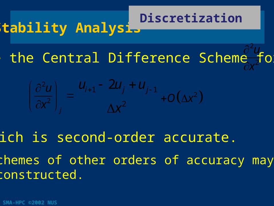
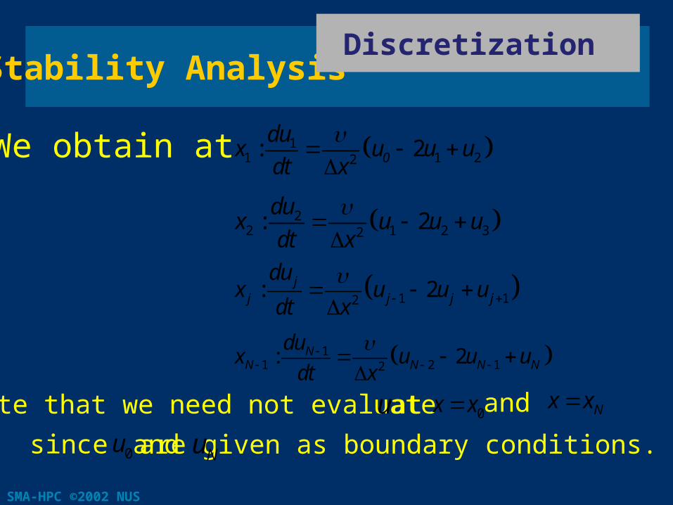
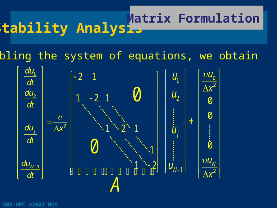
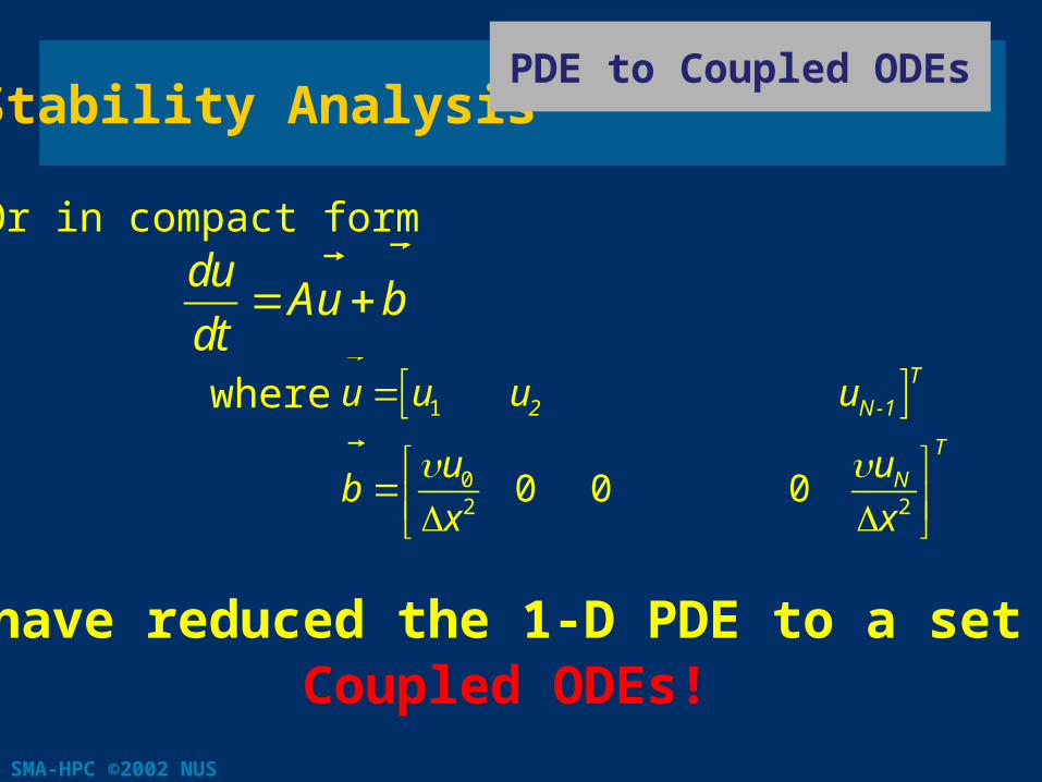
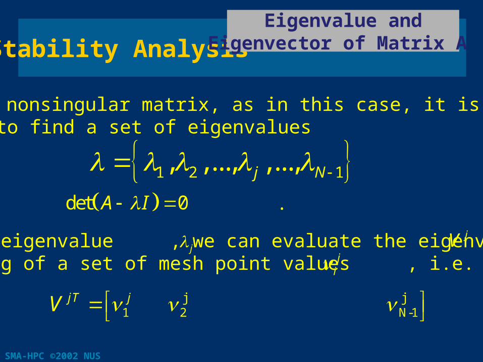
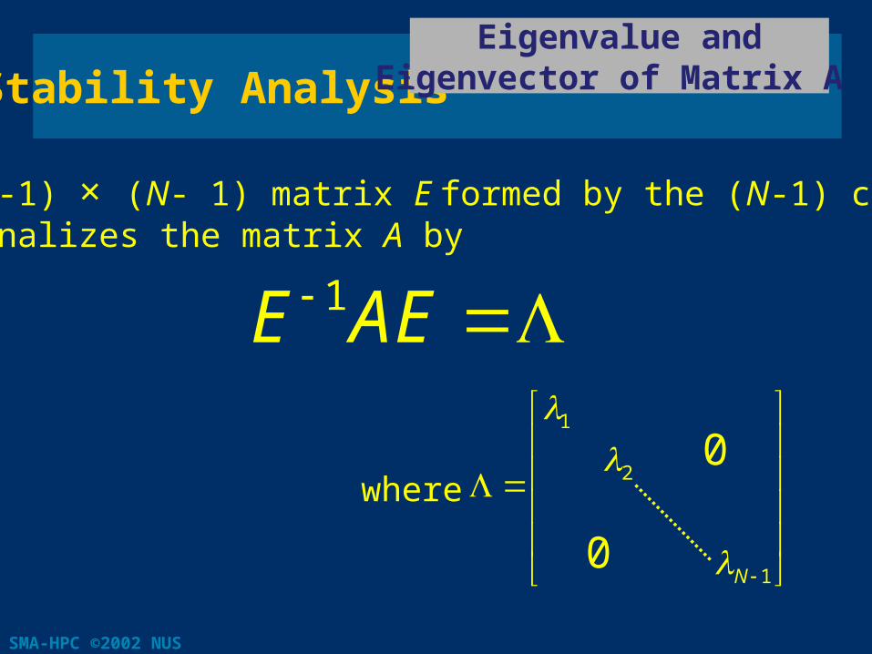
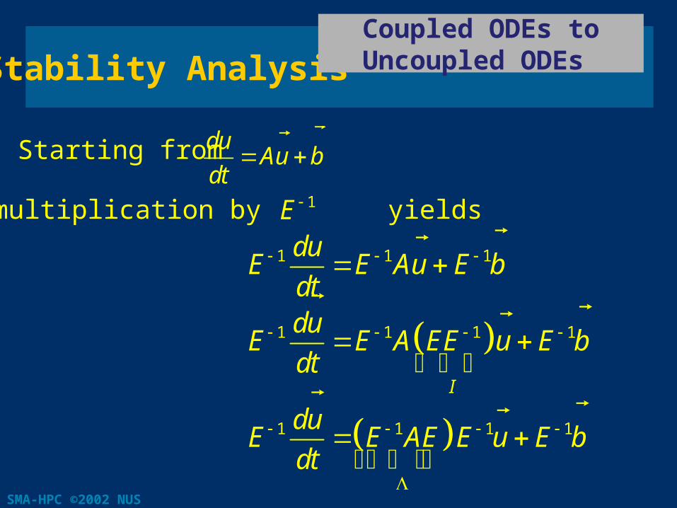
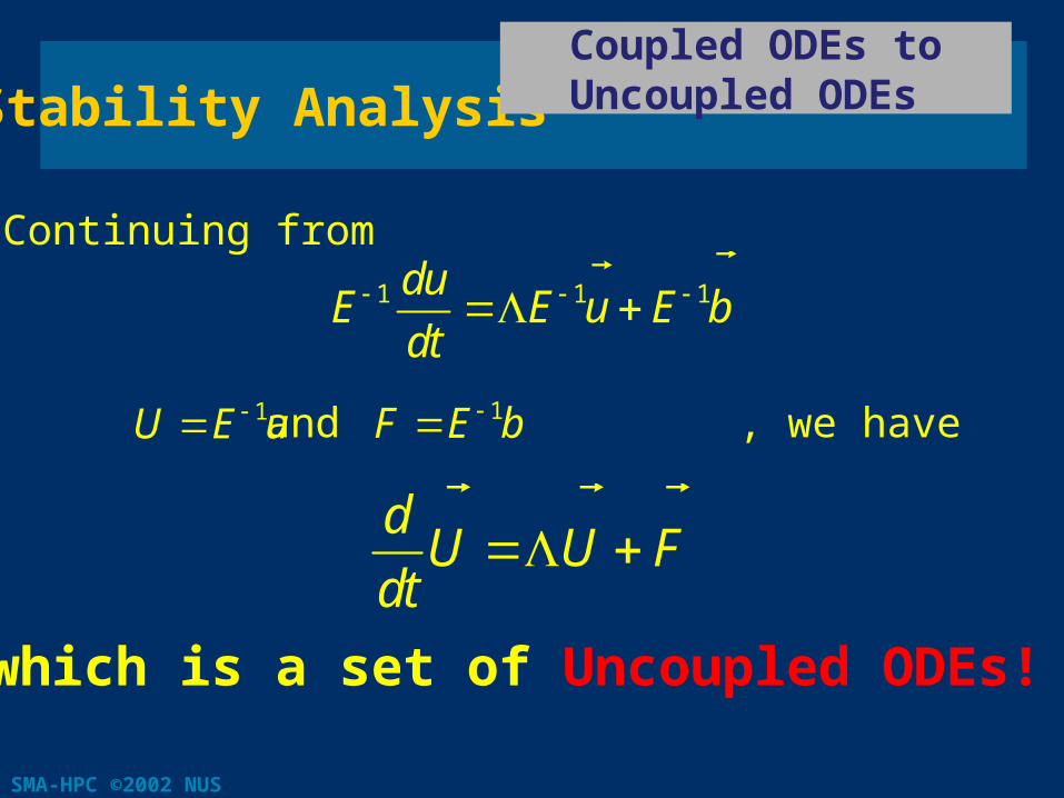
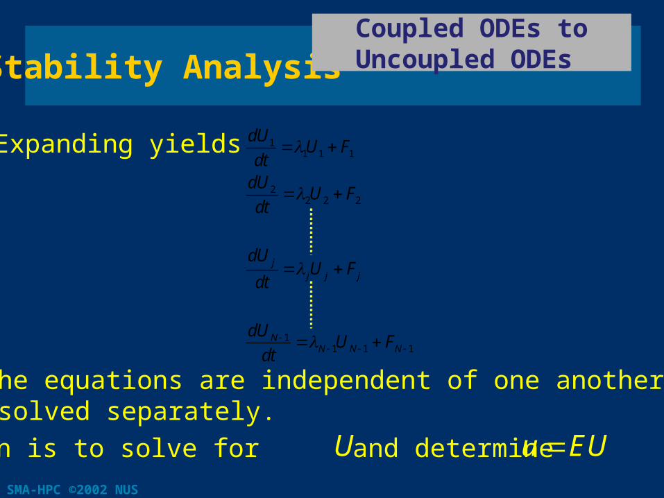
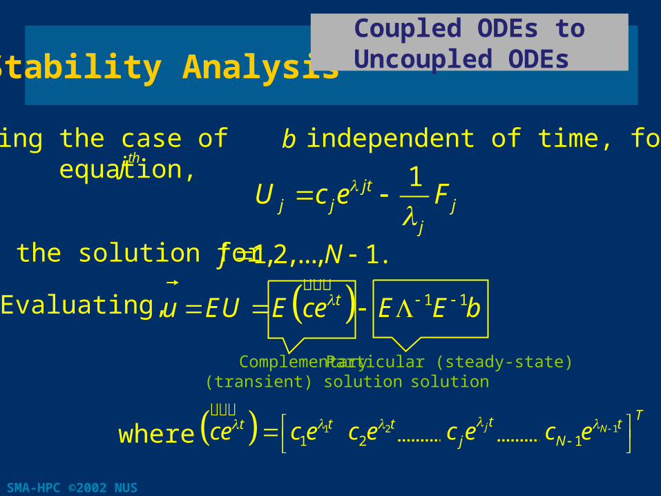
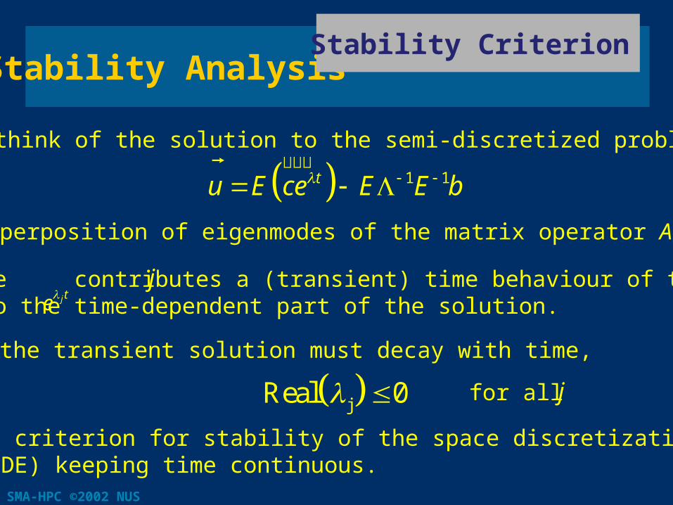
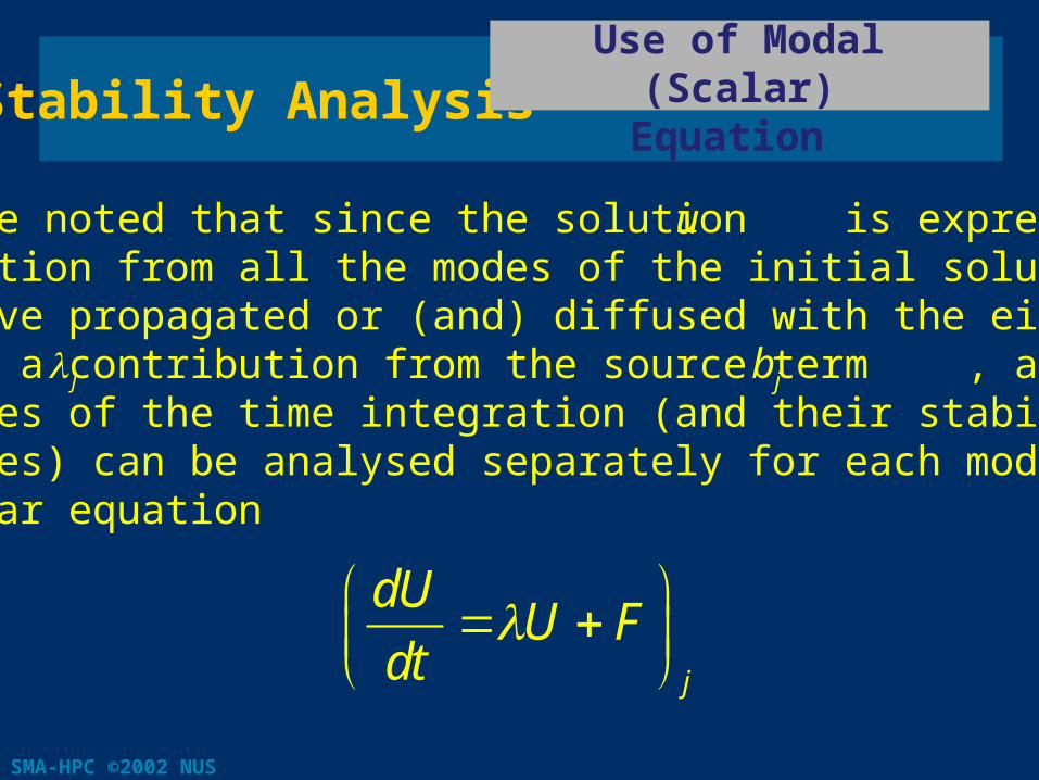
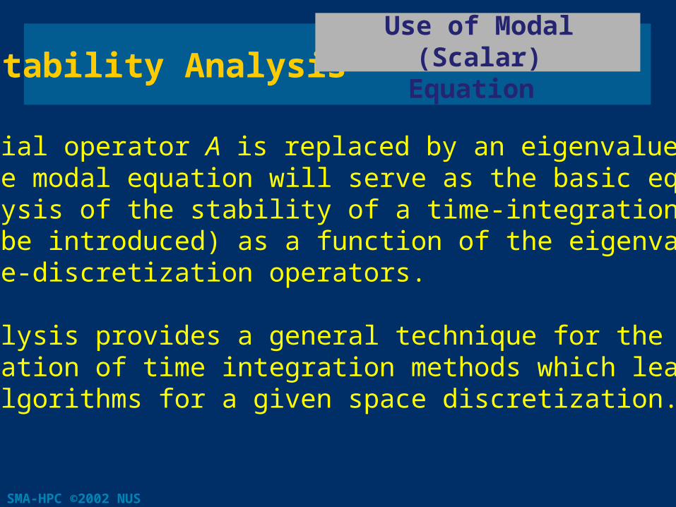
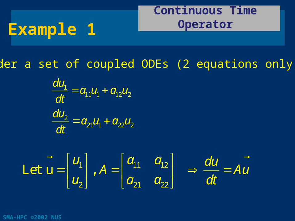
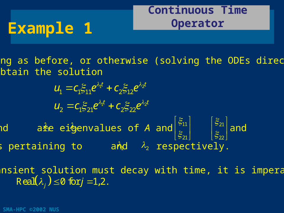
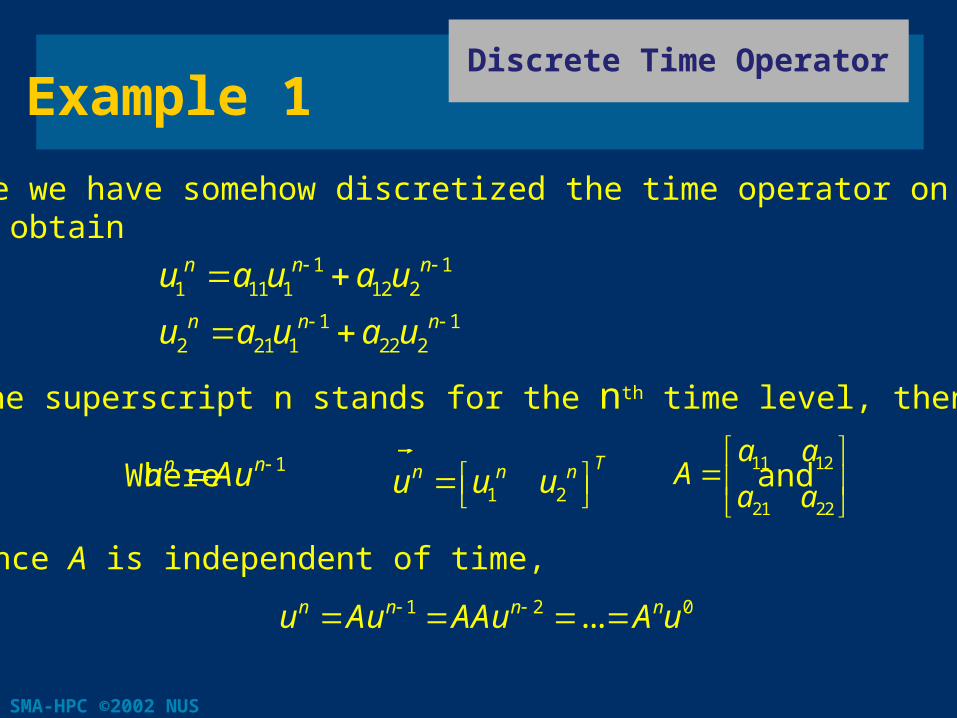
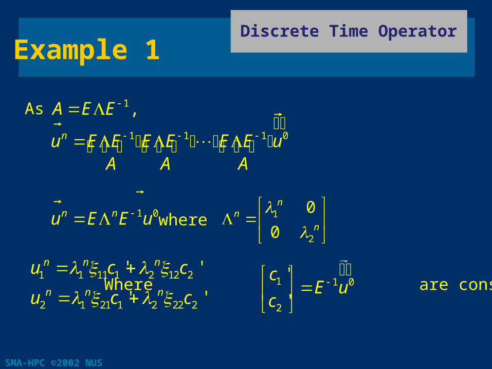
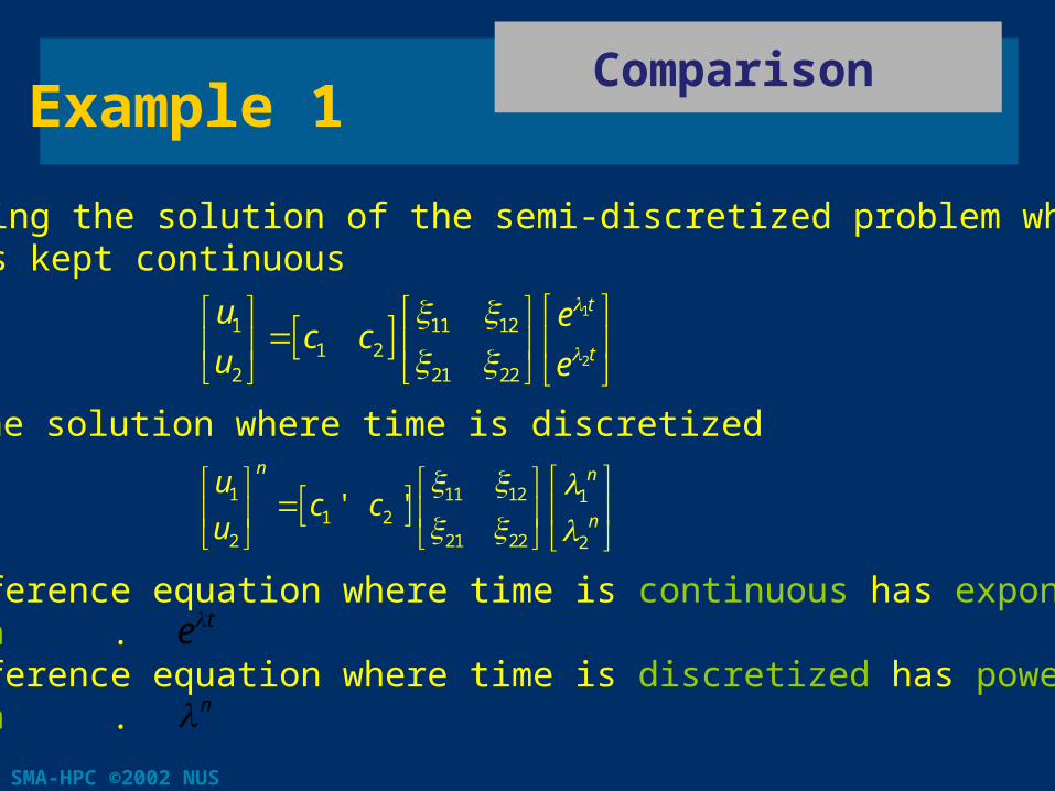
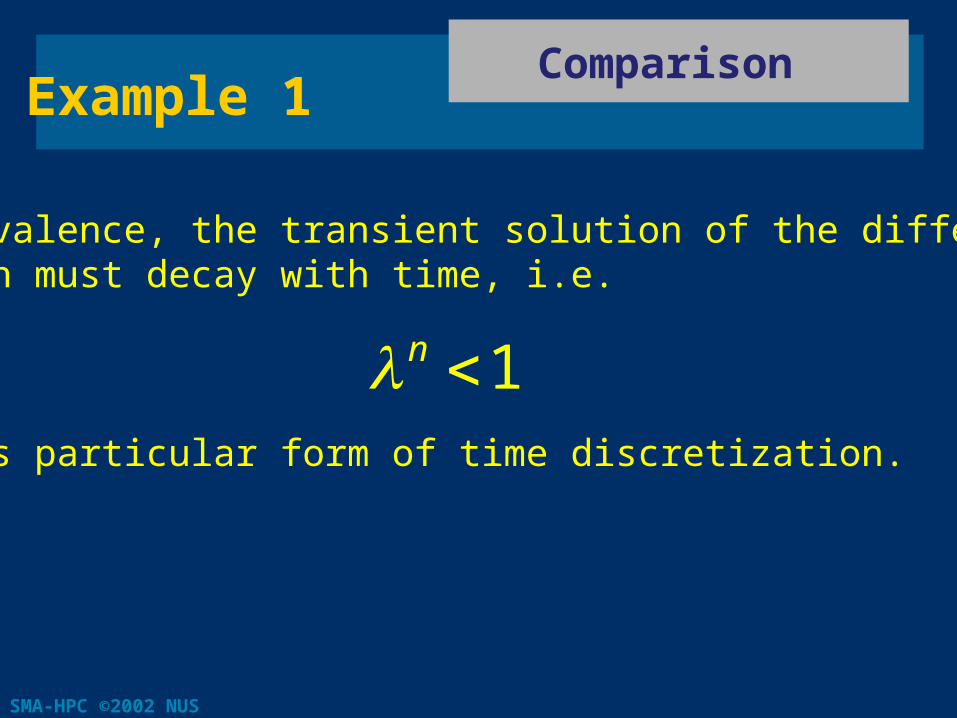
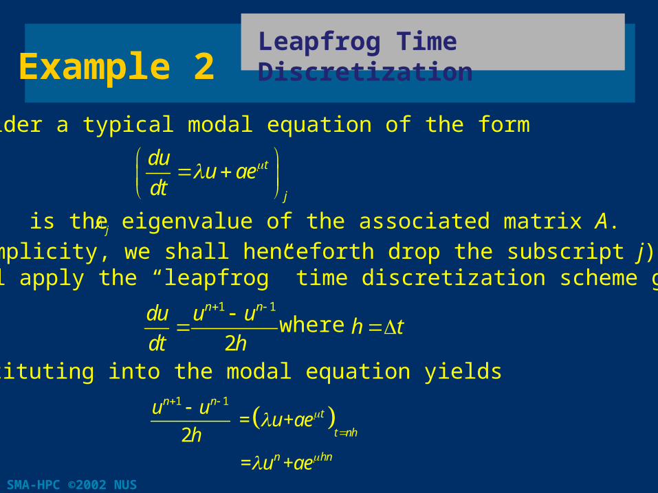
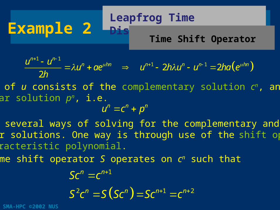
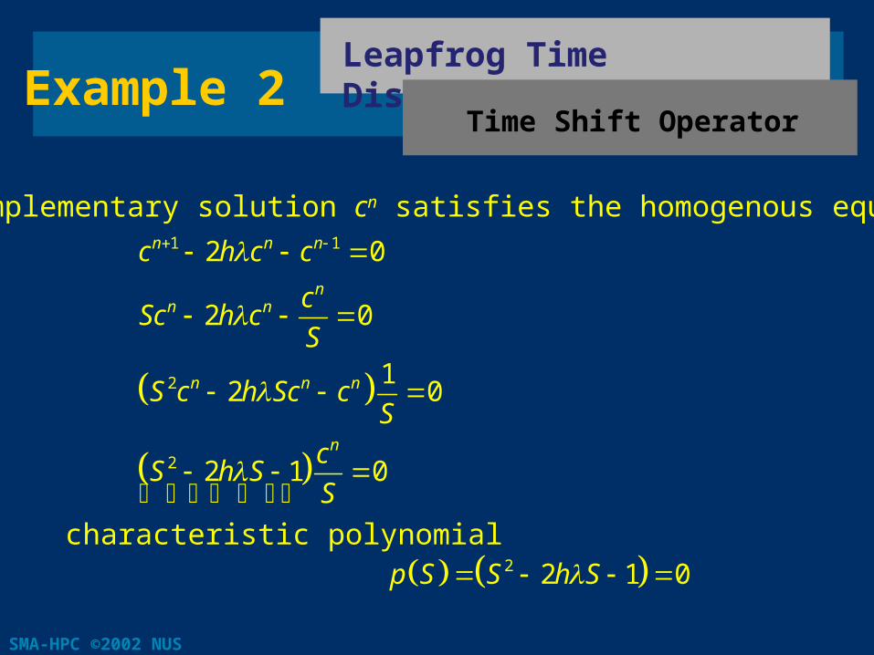
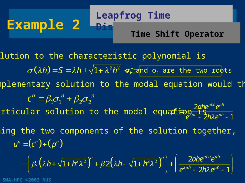
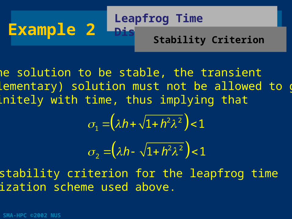
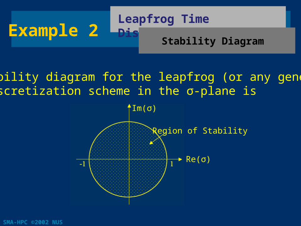
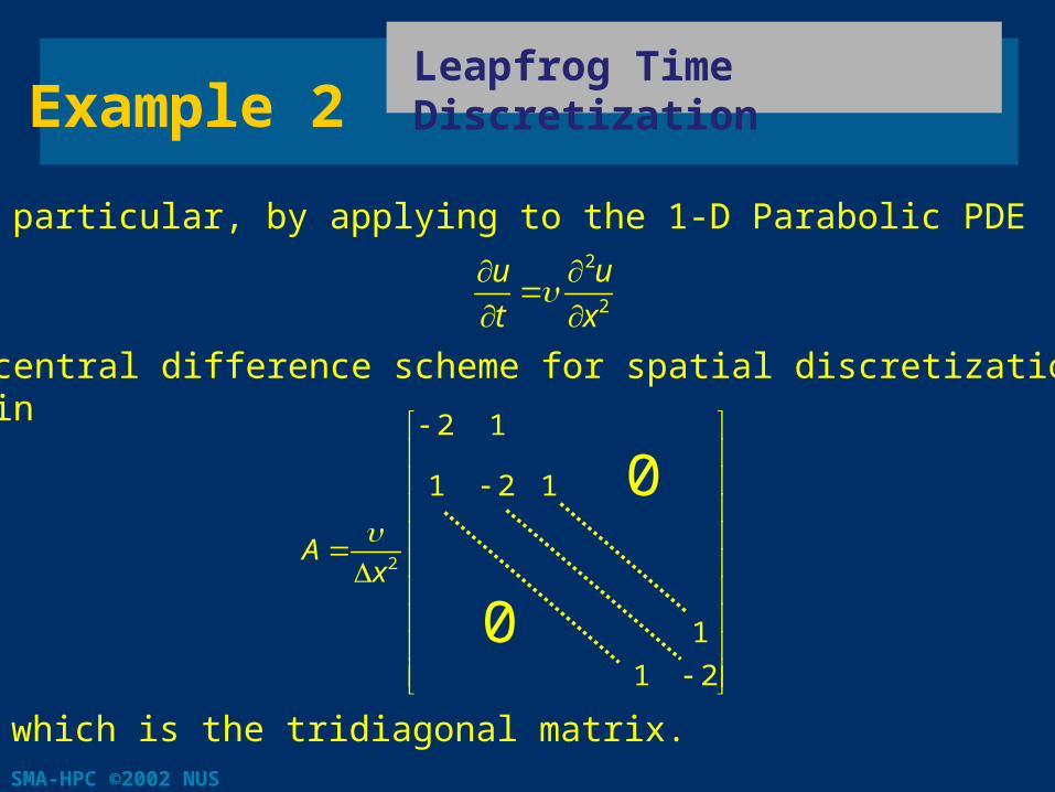
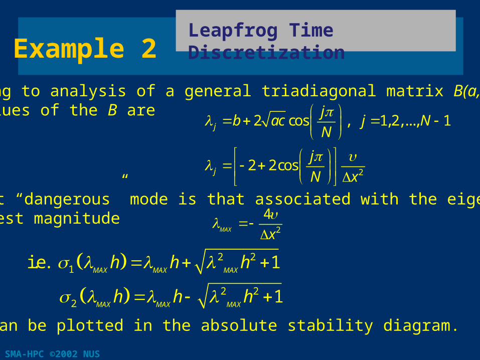
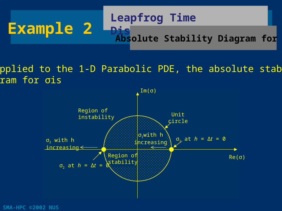
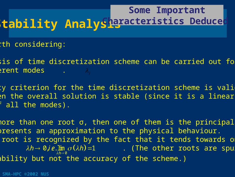
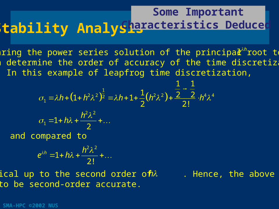
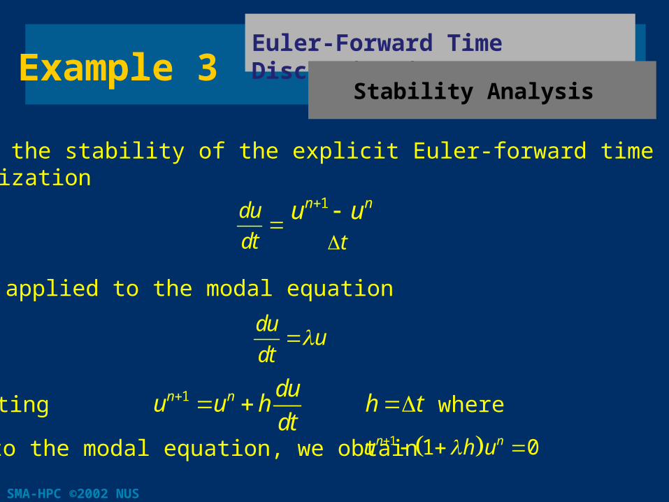
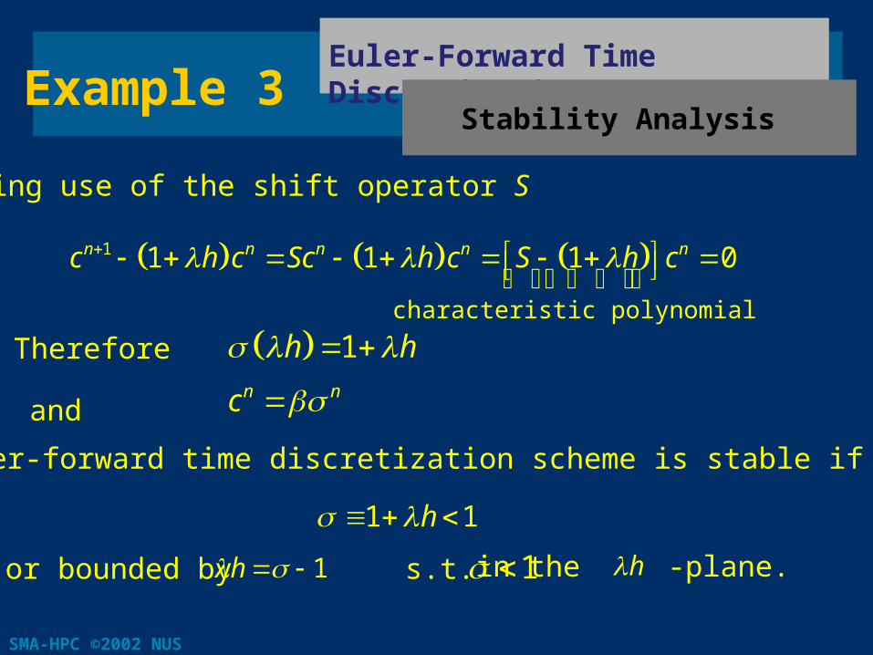
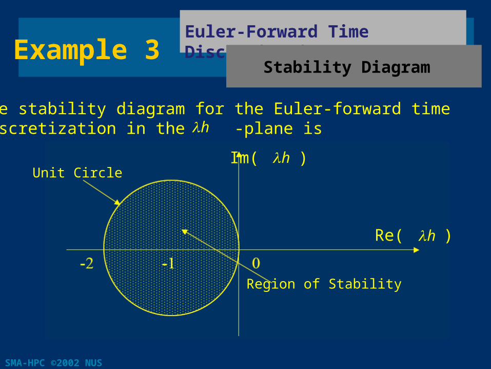
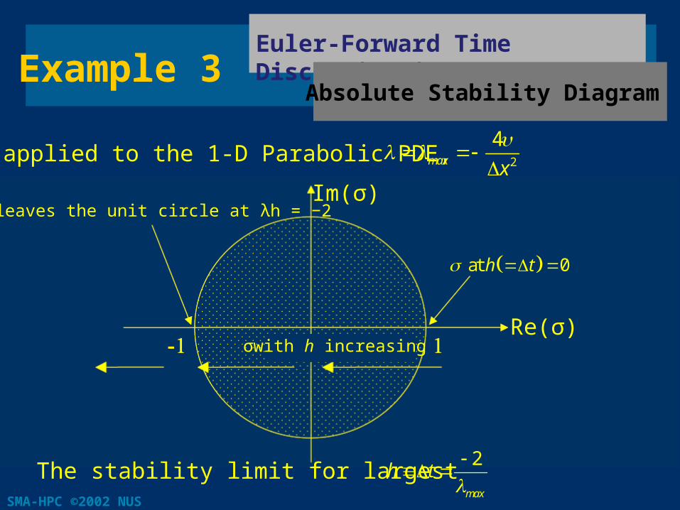
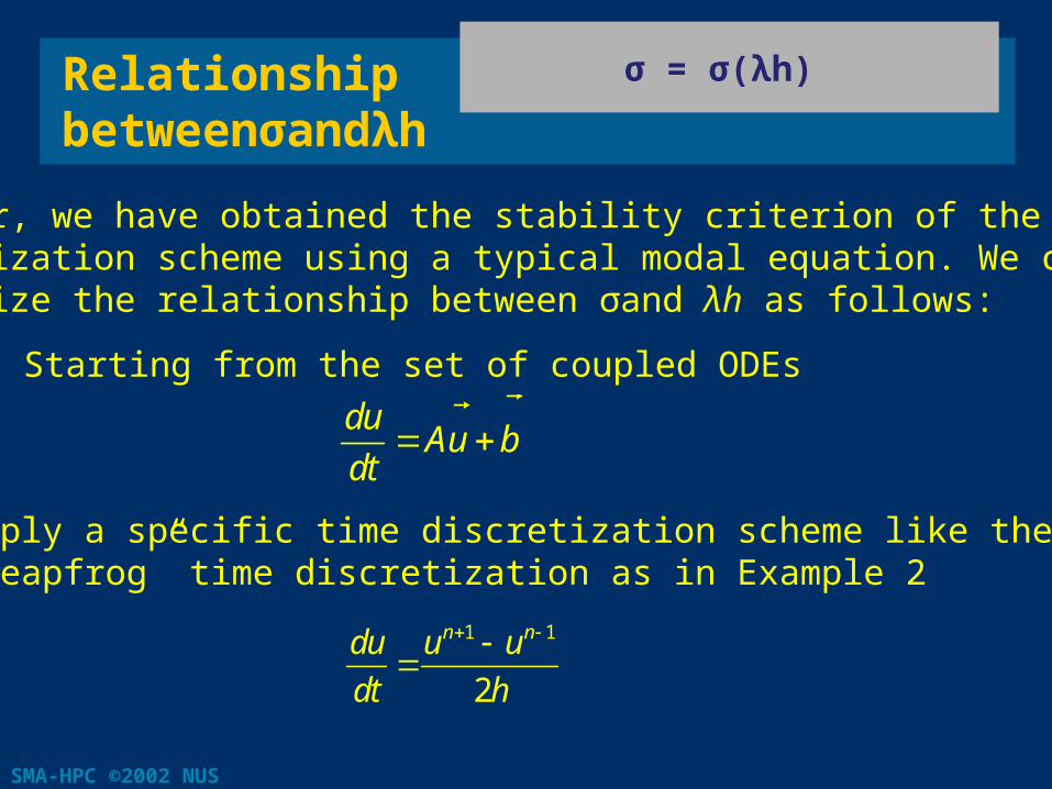
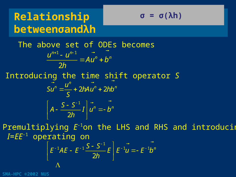
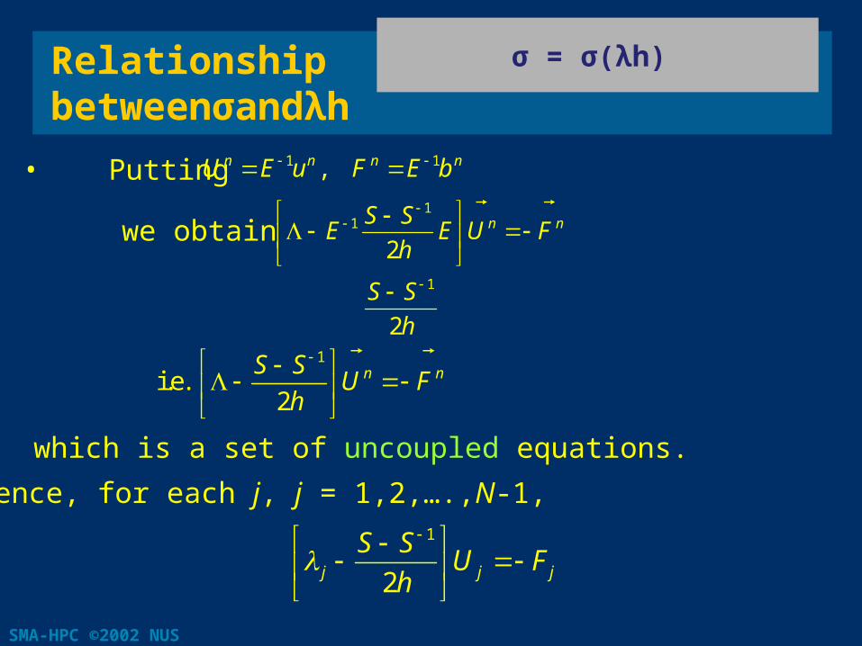
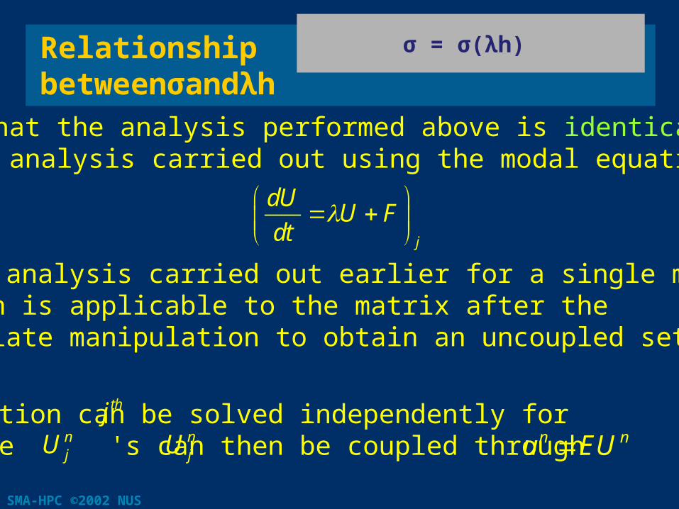
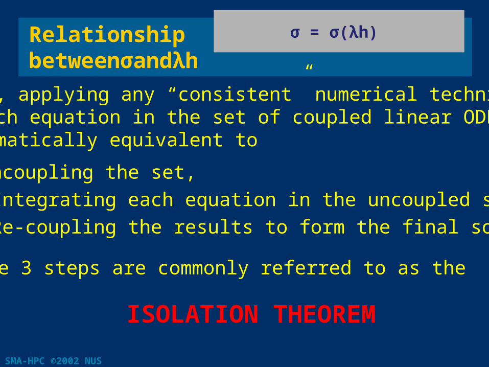
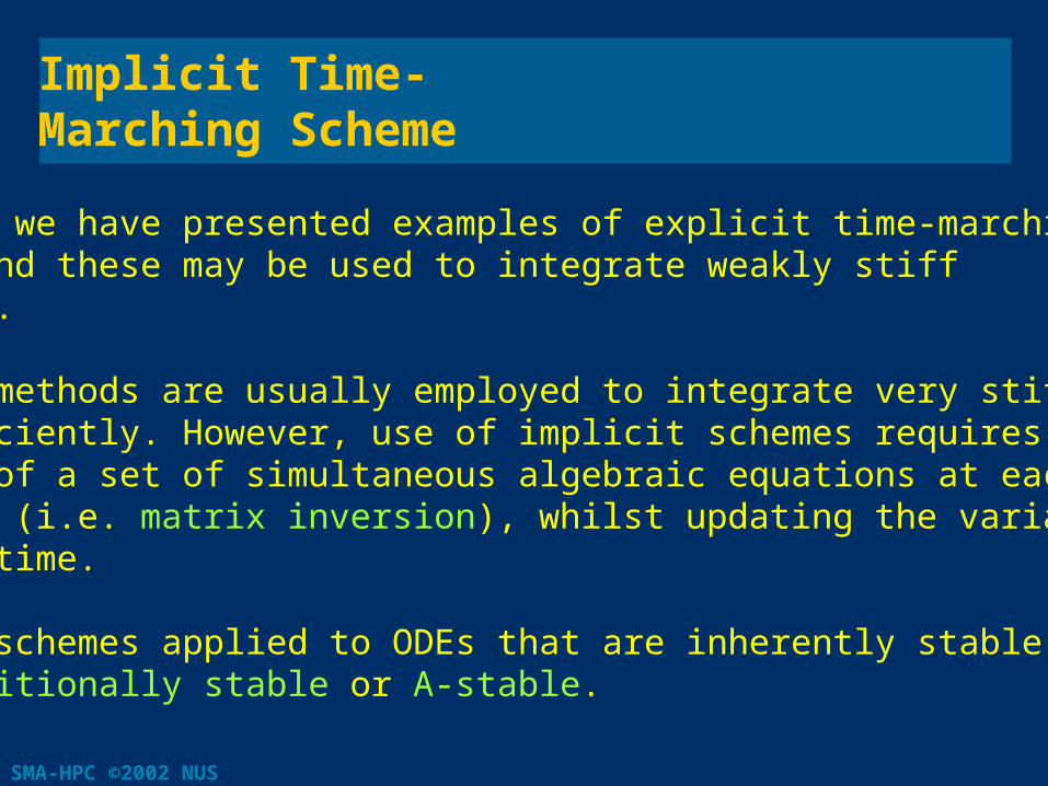
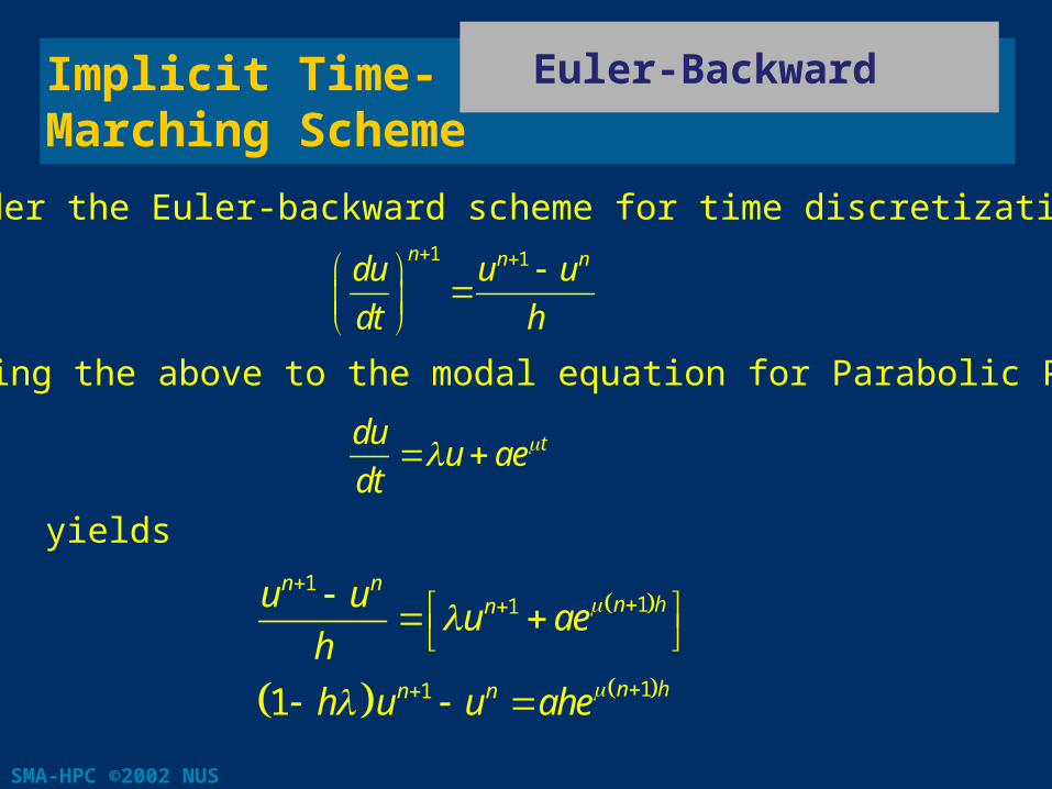
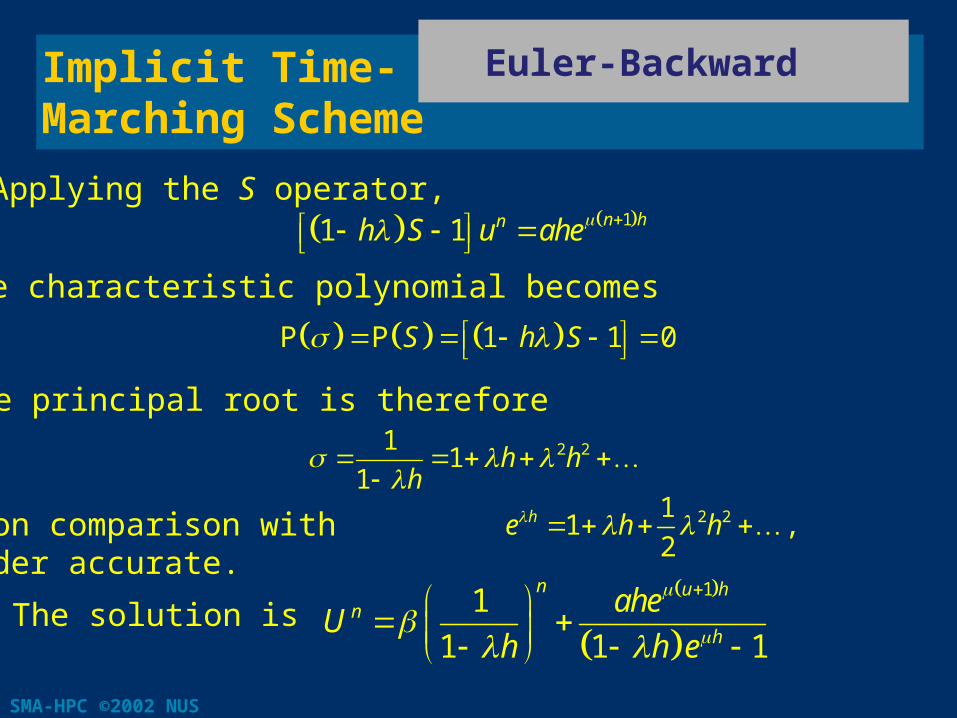
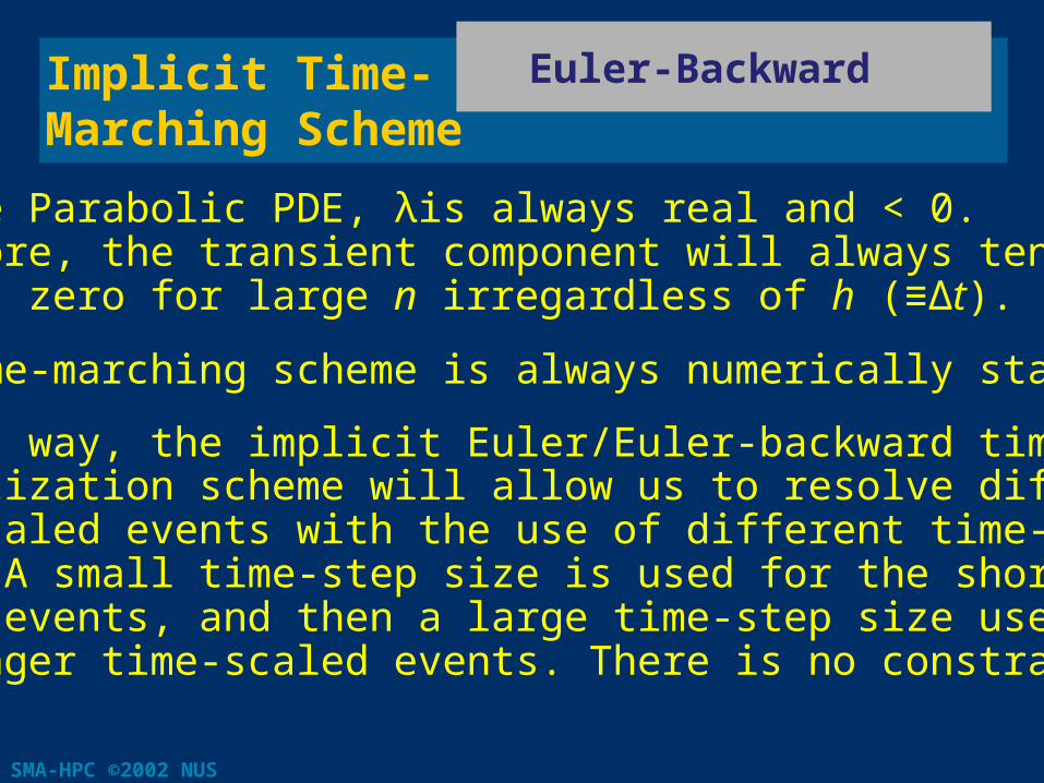
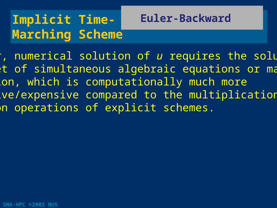
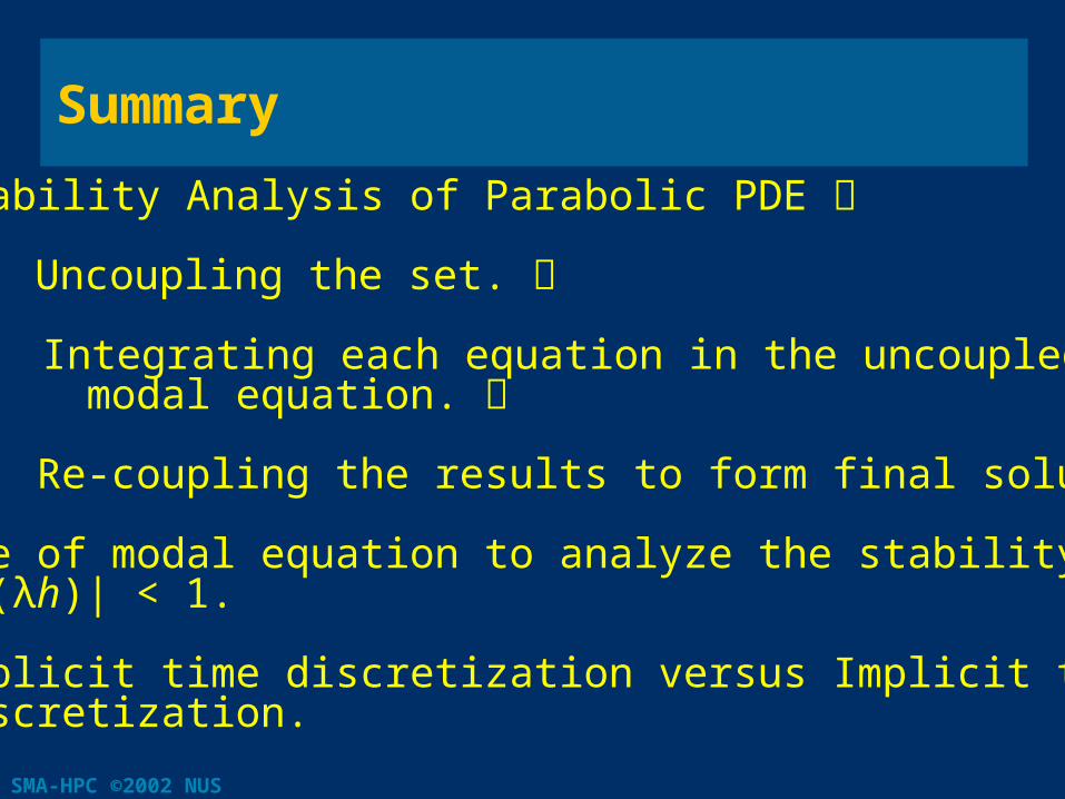


![[Sách] Bí quyết gây dựng cơ nghiệp bạc tỷ , Adam Khoo](https://img.pdfslide.tips/doc/110x75/58ea12e51a28ab064e8b55c1/sach-bi-quyet-gay-dung-co-nghiep-bac-ty-adam-khoo.jpg)