Embed Size (px)
Citation preview
8/8/2019 19630001806_1963001806 (Metodo Numerico de Diseno)
http://slidepdf.com/reader/full/196300018061963001806-metodo-numerico-de-diseno 1/36
NASA TN D- 1 5 6 2
TECHNICAL NOTE A '
0-1562
METHOD FOR DESIGN O F P U M P I M P E L L E R S U SING A
HIGH-SPEED DIGITAL COMPUTER
By N o r b e r t 0. S to c k m a n a nd John L. K r a m e r
L e w i s R e s e a r c h C e n t e rCleve land , Ohio
NATIONAL AERONAUTICS AND SPACE ADMINISTRATION
WASHINGTON January 1963
-. . ' J
8/8/2019 19630001806_1963001806 (Metodo Numerico de Diseno)
http://slidepdf.com/reader/full/196300018061963001806-metodo-numerico-de-diseno 2/36
8/8/2019 19630001806_1963001806 (Metodo Numerico de Diseno)
http://slidepdf.com/reader/full/196300018061963001806-metodo-numerico-de-diseno 3/36
use of this method for the design of centrifugal pumps.it is desirable to determine the specific flow equations and design methods forthe incompressible f l o w in pump impellers, and to detail the procedures for high-speed digital-computer use.
method.
To facilitate this use,
This report presents the development of such a
The basic flow equations are derived from the equations of motion for amean-flow surface that extends from impeller hub to shroud. The required equa-tion for stream tube volume flow is derived from continuity considerations. An
approximate method of computing blade-surface flow properties is also derived.
In addition, the overall pump-design problem is discussed. Methods of ob-taining quantities needed in the design calculations are given, and the numericalmethods of attacking the design equa,tions nd a block diagram for a digital-computer program are presented. Finally, a numerical example illustrating theuse of the method and suggestions for further use are given.
DESIGN PROBLEM
The general design problem can be considered from two points of view,namely, the engineering and the mathematical. The engineering approach is:Given a f l o w rate and a head rise, find a pump that will produce the desiredperformance with maximum efficiency. The mathematical approach is: Given the
distribution of some flow property, such as velocity, on the boundaries (hub,
shroud, and blade surfaces) and assumptions regarding the type of flow, find theimpeller geometry that will result in these flow properties.
Fundamentally, the problem is an engineering one; that is, the pump mustproduce a certain flow and a certain head rise and possibly meet other restric-
tions, such as a maximum allowable diameter, a specified rotative speed, and soforth. Commonly, the engineering goal is achieved through the combined use ofa certain amount of mathematical design, the designer's art and experience, andpossibly development.
The ideal approach would be to convert the engineering specifications intoinputs f o r a complete mathematical design, to specify desirable flow properties
along the impeller boundaries, and to compute the geometry of the impeller.
Unfortunately, complete three-dimensional design methods, such as suggestedin reference 4, are long and complex.is available for the computation, the setting up of the problem for the computer
would be a long and tedious process. An exact two-dimensional method is used inreferences 5 and 6 to obtain blade-to-blade properties in a prescribed pump
stream-tube impeller geometry without and with splitter vanes, respectively.This method gives an adequate picture of the flow in the leading-edge region andwould be useful for cavitation considerations; however, the exact solution isquite complex and involves considerable calculations. It is important, there-fore, that rapid easy-to-use methods accurate enough for engineering purposes bedeveloped. Two such methods of obtaining flow properties on the blade surfaces
are given in references 1 and 7. In references 5 and 6, it was found that these
Even when a high-speed digital computer
2
8/8/2019 19630001806_1963001806 (Metodo Numerico de Diseno)
http://slidepdf.com/reader/full/196300018061963001806-metodo-numerico-de-diseno 4/36
methods gave reasonably accu rate r e s u l t s throughout most of th e bla de passage.
Although th es e methods a re of l im i t ed value for s t u d yi n g c a v i t a t i o n c o n d it i o ns ,
t hey a r e su f f i c i e n t f o r eddy de t ec t i o n and fo r bounda ry - layer and l oad i ng s t ud i e s
e xc ep t i n t h e i mm ed ia te v i c i n i t y o f t h e t r a i l i n g edge and i n a r e g i o n n e a r t h e
l e a d i n g edge t h a t e x te n ds f u r t h e r i n t o t h e i m p e l le r as t h e ang l e of a t t a ck dev i-
a t e s f rom t he des i gn va l ue .
Veloc i ty Gradien t
The hub-shroud d esig n method pre sent ed herein (w i th opt io na l blad e-su rfa ce
computat ions) i s ayiother such rapid and easy-to-use methnd.
d e s i g n e r t o p ro ce ed from a known s tr e a m li n e and i t s v e l o c i ty d i s t r i b u t i o n t o an
ad j acen t s t r eam l i ne and i t s ve l o c i t y d i s t r i bu t i o n . Thus, g i ven t h e cond i t i ons
a long th e hub , th e e n t i r e hub-shroud p r o f i l e is hu j l t . 1 q by prcceeding frcm t h e
hub s t r eam l i ne t o t h e nex t s t r eam l i ne , and s o on, u n t i l t h e s h ro ud i s reached.
C onve rs ion o f t h e pump sp ec i f i ca t i o ns i n t o i npu t fo r t h e des ign c a l cu l a t i on s i s
d e sc r ib e d i n t h e DESIGN I"TS ec t i on .
It enzb l e s t hc
DESIGN EQUATIONS
Stream Tube Volume Flow
The coord ina tes o f an unknown s t ream l ine a r e re l a t e d t o th ose of an ad jacen t
I n t h e d e r iv a t i o n of t h i snown st re am li ne by a form of th e con t inu i t y equa t ion .
equa t ion , i t i s assumed th a t sur face s of revolu t io n ob ta ine d by ro ta t i ng stream-l i n e s a b ou t t h e i m p e l le r axis a r e s t r eam su r faces and t h a t all passages between
blades ca rr y t h e same volume flow. Then t h e equ ation f o r the volume flow pe r
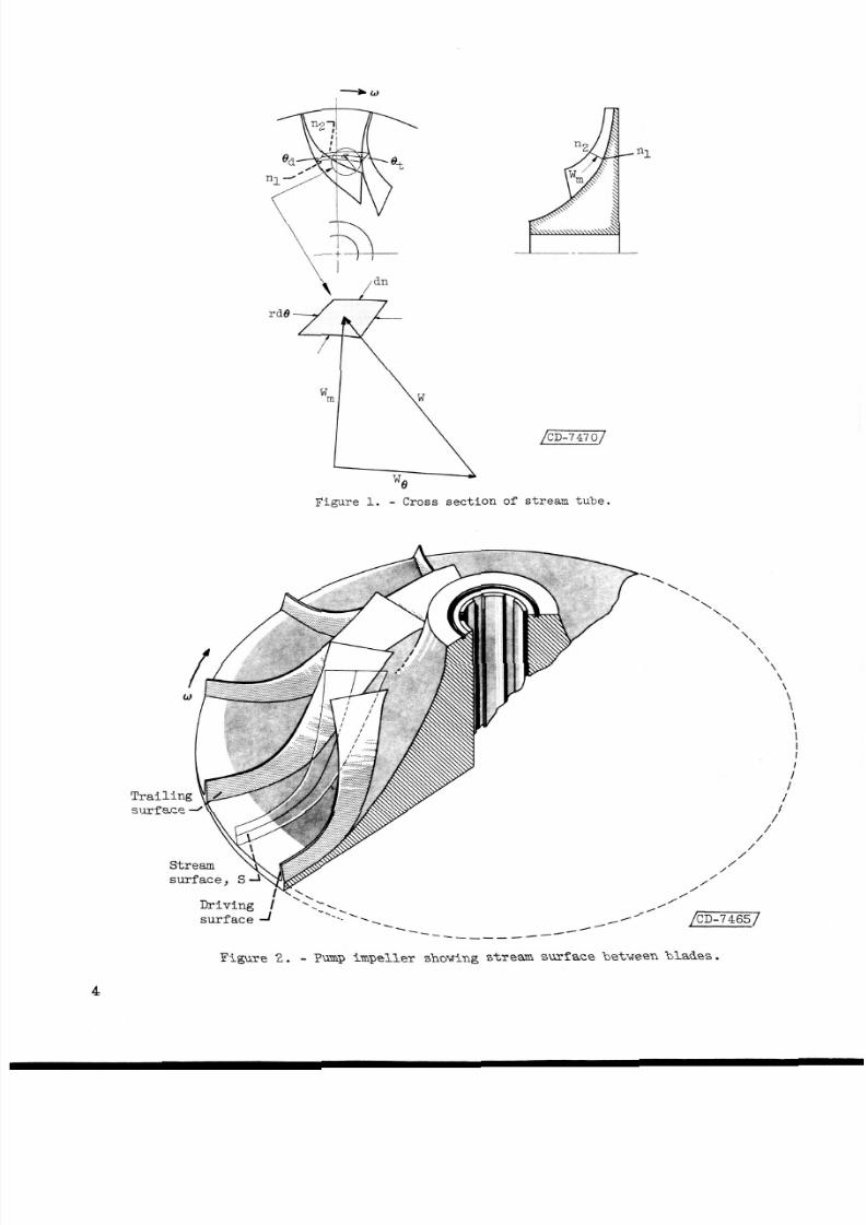
un i t b l ade pas sage AQ/M through a cross sec t ion of a stream tube bounded by
adja cent sur fac es of revo lu t ion nl and n2 and by ad ja cen t b l ades Bt and
8d, as shown i n f ig ur e 1, i s obtained by
where A i s t h e area of a c r o s s s e c t i o n of st ream tube everywhere normal t o t h e
mer id iona l or t h rough-f low d i rec t ion , Wm
velocity component and i s a func t ion of n and 8, and r i s t h e r a d i a l d i s -
t a n c e t o t h e c e n t e r of t h e e le me nt and i s a func t i on of n.
de f i ned i n append ix A. )
i s t he m er i d i ona l or through-f low
(All symbols are
The ve lo c i ty - grad ien t equa t ion (which i s der ived i n appendix B) i s used t o
o b t a i n t h e v e l o c i t y o n a new streamline when i t i s known on an adjacent s t ream-
l i ne . S i m p l i f i ca t i o n of t he exac t t h ree -d i mensi ona l equa t i ons o f m ot ion t o as im p le ve l oc i t y -g ra d i en t equa ti on i s accomplished i n t w o m aj or s t e p s . I n t h e
f i r s t s t e p , the problem i s reduced t o t w o dimensions by considering the flow on
a known str ea m su rf ac e S ( f i g . 2 ) t h a t extends from hub t o shroud throughout
3
8/8/2019 19630001806_1963001806 (Metodo Numerico de Diseno)
http://slidepdf.com/reader/full/196300018061963001806-metodo-numerico-de-diseno 5/36
“1
Figure 1. - Cross sec t ion of stream t u b e .
\)’--\,\\
\
\
\\
\\
\\\IIIII
IIi
Figure 2 . - Pump impeller showing stream sur fac e between b lades .
4
8/8/2019 19630001806_1963001806 (Metodo Numerico de Diseno)
http://slidepdf.com/reader/full/196300018061963001806-metodo-numerico-de-diseno 6/36
t h e impel l e r . Mathemat ica l ly , t h i s sur fa ce can be any stream su r f ac e be tween
blades. It i s r ea sonab le t o assume t h a t t h e mean f low fol lo ws a mea??blade s u r -
fa ce throuShout t h e gu ided por t ion of t he impel l e r .
deviates from the mean blade su r fa ce f o r nonzero ang l e o f a t t a ck a d , a t t h e
o u t l e t , i t d i f f e r s because o f s l i p .
and a re d i scussed i n t h e s ec t i o n on Bl ade P rope r ti e s .
A t t h e i n l e t , t h e s ur f ac e
These two factors can be t aken i n t o accoun t
I n g e n e r a l , f l o w p r o p e r t i e s a r e f un c ti on s o f 6, r, and z; bu t on t he su r -?axe, 6 i s a f i inct ion of r and z. Therefore, t h e f low on th e su r f ac e i s a
func t ion of r and z on l y ; t ha t i s , i t i s mathematical ly two dimensional . As
a r e s u l t , t h e d e s ig n c a l c u l a t i o n s can be s e t up as i f t h e f l ow were i n an r-zo r merir7inna.l p?a.ne. A meridional plane i s a. plane t h a t c o n ta i ns t h e i m p e l l e r
a x i s , b u t i t i s n o t a p h y s i c a l l y me an in gf ul p la ne i n t h e f l o w f i e l d ( e x ce p t i n
t h e ca se w he re t h e r e i s no r e l a t i v e c i r c u m f e r e n t i a l v e l o c i t y ) .
working i n th e mer id iona l p l ane i s t h a t t h e m e ri di on a l s t r e a m l i n e p i c t u r e i s at r u e r e p r e s e n t a t i o n o f t h e t hr ou gh f l o w a s s oc i a te d w i th t h e s u r f a c e
An advantage of
S.
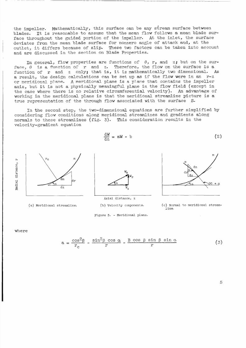
I n th e second s t e p , t h e two-dimens iona l equa t ions are f u r t h e r s i m p l i f i e d by
cons ider ing f lo w condi t ions a long mer id iona l s -breamlines and gr ad ie n t s a longn or ma ls t o t h e s e s t r e a m l i n e s
ve l oc i t y -g rad i en t equa t i on
( a ) M er i d i ona l s t r eam l i ne .
( f i g . 3 ) . This c o ns id e ra ti on r e s u l t s i n t h e
- Iw - a W - bdn
Axial d i s t ance , z
( b ) Velocity components.
F i gu re 3. - Meridional plane.
where
I
( c ) Normal t o merid ional s t ream-
l i n e .
coszp s inzp cos a - B cos s i n p s i n aa = - -
r r ( 3 )
5
8/8/2019 19630001806_1963001806 (Metodo Numerico de Diseno)
http://slidepdf.com/reader/full/196300018061963001806-metodo-numerico-de-diseno 7/36
and
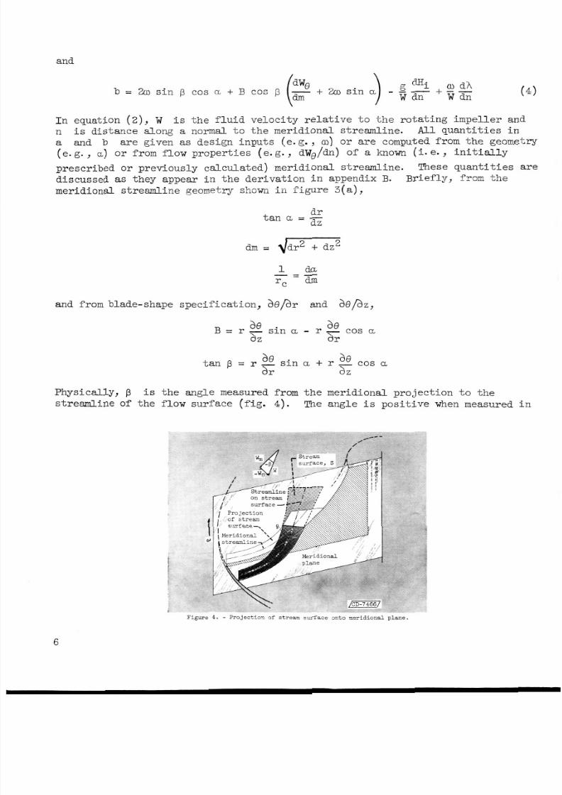
b = 2co s i n p COS a. + B cos p (2 ZCU s i n + - -W dn W dn
I n equation (2), W i s t h e f l u i d v e l o ci t y r e l a t i v e t o t h e r o t a t i n g i mp e l l er and
n i s distance along a normal t o th e meridional s t ream line. All q u a n t i t i e s i na and b
(e. g. , ) or from flow prope rt ie s (e. g. , dWQ/dn) of a known (i. . , i n i t i a l l y
prescribed or previously c alc ula ted ) meridional s t reamline.discussed as they appear i n t he der iva t ion i n aFpendix B. Brief ly , from th e
meridional stre am line geometry shown i n f ig ur e 3 ( a ) ,
ar e g iven as design i nput s (e. g ., cu) or are computed from the geometry
These quant i t ies are
d rt a n a. =-
dz
d m = 4
and from blade-shape sp ec ifi ca tio n, &/a, and ae / a z ,
B - r - s i n a -8 r - c o s aea, a,
Physical ly , ps t reaml ine of th e f low surfac e ( f ig .
i s th e angle measured from t h e meridional pr oje ct io n t o t h e
4). The angle i s p o s it iv e when measured i n
I
~ on stream
Figure 4. - Projec t ion of stream surface onto meridional plane.
6
8/8/2019 19630001806_1963001806 (Metodo Numerico de Diseno)
http://slidepdf.com/reader/full/196300018061963001806-metodo-numerico-de-diseno 8/36
t h e d i r ec t i on of ro t a t i on . The r em a in ing qua n t i t i e s i n b a r e o b t ai n e d asfo l lows: We equa l s W s i n p. j a, t h e r o t a t i v e s pe ed of t h e i m p e l le r , i s pre-
s c r i b e d ; - - here i s obta ined from a p r e s cr i b ed d i s t r i b u t i o n of H i
a t t h e i n l e t and An i s ob t a i ned f r o m cont inu i ty j and -
d R i M i
dn dn&¶i
as f o r -n
'
dh ah
dn =
With th e two equat i ons, ve l oc i t y ( eq . ( 2 ) ) and con t i nu i t y ( eq . (1)): t h e
hub-shroud p r o f i l e can be cons t ruc t ed f r o m a g iven mer id iona l s t reaml ine and i t s
v e l o c i t y d i s t r i b u t i o n and a given blade shape.
su r f ace th roughou t t he i m pe l l e r i s of necessit .? nht.nAned z s p a r t ef t h e d z ~ 2 . g ~
c a l c u l a t i o n .
The ve loc i ty on the s t ream
Head
The s t a t i c head ha long a st reaml ine can be obtained from equat ion (B22):
where Hi i s t h e i n l e t t o t a l head t h a t i s given f o r each s t reaml ine .
The t o t a l head a long a st re am lin e can be computed from equati on ( B 2 8 ) ;
This completes the incompressible nonviscous flow c a l c u l a t i o n s on t h e streams u r f a c e S.
Blade-to-Blade Calculat ions
Approximate b lade-sur face ve lo c i t i es and s t a t i c heads can be ob ta ined f rom
They pro-
equa t i ons ((3) o ( c y ) .assumption 6f a l i n e a r v a r i a t i o n o f s t a t i c head f ro m b l a de t o bl ad e .
v i d e r e s u l t s o f s a t i s f a c t o r y a c cu ra cy ex c ep t i n t h e l ead i ng - and t r a i l i n g -ed ge
r e g i o n s o f t h e bl a d es . I f more exac t r e s u l t s a r e r equ i r ed , t h e b l ade- t o -b l ade
an a l ys i s method of r e f e r e n c e s 5 o r 6 can be used.
These equa t ions a r e der ived i n appendix C w i t h t h e
DESIGN l2E"S
The equa t ions prese n ted i n th e prev ious sec t io n enable computa tion of th e
in te rna l - f low cond i t ions and th e shroud shape of a pump im pe lle r provided th a t
t h e fo l l ow i ng qu an t i t i e s a r e known, t h a t i s , given or pr esc rib ed : volume flow
7
8/8/2019 19630001806_1963001806 (Metodo Numerico de Diseno)
http://slidepdf.com/reader/full/196300018061963001806-metodo-numerico-de-diseno 9/36
ra te , Q; head r i s e , A€€;n l e t - t o t a l - h e a d d i s t r i b u t i o n , Hi; i n l e t - p r e w h i r l d i s -
t r i b u - t i o n , A r o t a t i v e s pe ed , cu; meridional contour of some streamline such as
s u r f a c e i n terms of t h e curv atu re components, &I/&
ness , tn or t e j the number of blades , M; an d any d e v i a t i o n of t h e f l o w s u r f a c e
from t h e blade sur face such as s l i p o r a n gl e of a t ta c k.
the hub , r = r ( z ) ; v e l o c i t y a lo ng t h i s s t r ea m l in e , W = W(r,z); t h e mean bl ad eand &/a,; t h e b l ad e t h i c k -
me f lo w r a t e Q and the head r i s e DH w i l l usua l ly be g iven as pump
spec i f i ca t ion s . The ro ta t i ve speed cu i s sometimes given. I n general , w, Q,
&I,1, and are n o t d i r e c t l y r e l a t e d t o hub shape , ve l oc i t y a long th e hub,
bl ad e shape, and number of bla de s, s o t h e des igner has cons iderab le f reedom i n
p r e s c ri b in g t h e s e q u a n t i t i e s .
ever , cer ta in re la t io ns among the se qu an t i t i e s and Q and AI€ must be sa t i s -
f i e d .
A
A t t h e i n l e t an d a t t h e o u t l e t of t h e pump, how-
Outlet Conditions
A t the ou t le t , two equa t ions mus t be sa t i s f i e d . The f i r s t i s E u l e r ’ s t u r -bine equat ion:
I n equation (5), 7 i s t h e h y d ra u l i c e f f i c i e n c y d e f in ed by
m a c t u a l
M i d e a l7 =
The hydra ulic ef fi ci en cy may be est ima ted from a c o n s id e r a t i o n of l o s s e s o rit may be ass igned from exper ience. The r o ta t i v e speed w may be chosen t o be
c o n s i s t e n t w i th o th e r f r e e c h o ic e s i n e q u a t io n ( 5 ) o r i t may be predetermined by
drive the pump.o the r cons idera t ions ; f o r example , t he w of a d i r e ct - d r iv e t u r b in e t h a t will
I f s l i p i s t o b e t ak e n i n to a c c ou n t, e q u at i on (5) becomes
where f ,
Blade Proper t ies .
i s t h e s l i p f a c t o r and i s d e f in ed a nd d i s c us s e d i n t h e s e c t i o n o n
The second equation i s t h e equat ion f o r volume f low ra te :
8
8/8/2019 19630001806_1963001806 (Metodo Numerico de Diseno)
http://slidepdf.com/reader/full/196300018061963001806-metodo-numerico-de-diseno 10/36
or Tor a r a d i a l o u t l e t when a = 90' and rs = r h
Q = ( W cos p ) a v ( f i r - Mte> (zs - Zh)av
The values of any quant i t ies (W , 6, e t c . ) n ee de d i n t h e d e s ig n must be p re -
s c r i b e d a t t h e o u t l e t t o be cons i s ten t wi th equa t ions (5 ) an d ( 6 ) and with any
ot he r constra . in ts imposed, f o r example, t h e exi s t in g geometry o f th e system i n
t o average val ues between hub and shroud. I n pr ac t ic e , however, th es e equa t ions
a r e u s ed t o o b t a i n i np u- t v a lue s on t h e p r e sc r ib e d s t r e a m l in e . The r e s u l t o f t h i s
r a t e from t h a t s p e c i f i e d . If t h i s i s a s ig n i f i c a n t d ev i a t i on , -th e p r e s c r i b e d
streamline and i t s r e l a t e d i n p u t c an b e a d ju st ed a f t e r a t r i a l design. This
adjustment can be repeat ed as o f t e n as required.
~ . : h i ~ hh e p i ~ q .e-Jle i jse& I n eqi ja t ions (5 ) and (5) the sid$ccyipt ay r e f e r s
prncedlx-e i s t h z t th e p m p Eay Frndixe 2 scxe::h=;t $:ffercnt head r:sc or flow
I n l e t C on di ti on s
There are f o u r p o ss i b l e s i t u a t i o n s t h a t may conf ront t h e des ign er a t t h e
pump i n l e t : (1)The upstream f low con di t ions a r e given, for example, when an
inducer precedes the pump; ( 2 ) the upstream geometry i s given, for example, a
p re d et e rm ine d i n l e t p ipe ; (3 ) t h e geometry immediately upstream of t h e pump i s
th e res po ns ib i l i t y of t h e pump des igner ; and ( 4 ) t h e r e a re no r e s t r i c t i o n s on t h e
i n l e t c o n d i t i on s , f o r example, i t i s t he res po ns ib i l i t y o f someone e l s e t o make
t h e i n l e t s e c t i o n f i t t h e pump.
For t e m ( Z ) , th e ups tream se c t ion can be ana lyzed ( f rom ess en t i a l ly th e
same equat ions as th ose used f o r th e pimp des ign) and the f low condi t ions are
then known.l e t se c t i on can be des igned by t he method of t h i s r ep or t (wi th ce r t a i n changes
because the re are no b la des ) then th e f low i s known as i n t h e s i t ua t i o n i n
i t em (1). Thus, f o r i n l e t c o n d it i o n s re q u ir e d as d e s ig n i n p u t , t h e r e are two
d i f f e r e n t s i t u a t i o n s , namely, i t em s (1)an d (4 ) .
o f c o n t i n u i t y
T h i s s i t u a t i o n i s now t h e same as i t e m (1). For i t e m ( 3 ) , t h e i n -
I n b o t h c as e s, t h e r e l a - t i o n s
AQ = (2f i r - M t e ) A y i W cos p (7)
where
r2 - rlAn = cos a1
e xc ep t i n t h e c a s e of a r a d i a l i n l e t a I 90a where
9
8/8/2019 19630001806_1963001806 (Metodo Numerico de Diseno)
http://slidepdf.com/reader/full/196300018061963001806-metodo-numerico-de-diseno 11/36
and c ons erv ati on of an gu la r momentum
m u s t b e s a t i s f i e d a t e ac h s t r e a m l in e f o r i t e m (1) an d a t some mean s tr ea ml in e f o r
i t em ( 4 ) .
Note tha t equa t ion ( 7 ) i s w r i t t e n f o r a s t a t i o n j u s t i n s i d e t h e i m pe l le r i n-
l e t r a t h e r t h a n j u s t upstream of t h e i n l e t an d, t h e r e f o r e , i n c lud e s b l a d e b lo c k-
age. A l s o , n o t e t h a t i n e q ua ti on ( 6 ) it i s assumed t h a t no work has y e t been
done on the f lu id a t t h i s s t at i on . Not a l l q u a n t i t i e s involved i n equa t ions ( 7 )
and (8) r e a c t u a l d e s ig n i n p u t a t every s t reamline .
l i n e ( u s u a ll y t h e hu b) h a s a W and r as input. Values of A a!id Hi (which
does no- t appear i n t h e equat ions) are r e q u i r e d i n p u t a t every s t re aml ine even
when upstream conditions are not prescr ibed. Values of p, te, and M a c r o s s
t h e i n l e t are i n c o r po r a t e d i n t o t h e b l a d e i n p u t . A ng le p i s t h e a n gl e of t h e
f l o w s u r f a ce n o t t h e b l a d e s u r f a c e , so t h a t when the se angle s a re not equa l
(when th e angle of a t t ac k i s n o t z e ro ) t h e b l a d e s h ap e a t t h e i n l e t must bespec iy ied in such a way as t o p r od uc e t h e r e q u i r e d v a lu e o f p.
Only the p resc r ibed stream-
Wnen equations ( 7 ) an d (8 ) a re used t o re la 'ce average condi t ions , as i n
i t e m (4),AQ becomes Q, an becomes ( r s - rh ) /cos a,, o r z s - Zh, and o t h e r
q u a n t i t i e s a r e a ve ra g es f ro m hub t o sh ro ud . V alue s f o r t h e p r e s c r i b e d s t r e a m l in e
a re estima ted from t h e hub-to-shroud average values. A f t e r a design i s made, t h e
i n l e t should be reexamined a t e ac h s t r e a m l i n e t o b e s u r e t h a t c o n di t io n s a re sat -i s f a c t o r y . I n p a r t i c u l a r , t h e blade ang le a t each s t ream l ine shou ld be such ast o p ro du ce t h e e x pe ct ed a n g l e o f a t t a c k ( u s u a l l y z e r o ). I f the expec ted ang le o f
a t t a c k i s n o t a t t a i n e d , some i n l e t c o n d i ti o n o r th e b lade shape a t t h e i n l e t must
be changed.
I n cases where t h e upstream f low i s known b e f o re t h e pump i s dssigned, the
s t r e am l in e s r e s u l t i n g f ro m th e d e sig n c a l c u l a t i o n must match the upstream stream-l i n e s a t t h e i n l e t . I f these two se ts oT s t reaml ines do no t match, some i n p u t
co nd it io n must be changed, and a new des ign ca lc u l a t i on ca r r ie d ou t . Elis proc-
ess i s r ep ea te d u n t i l a s a t i s f a c to r y m a tc h i s achieved.
Hub Shape and Velocity Distr ibution
A ft er t h e i n l e t and o u t l e t c o n di t io n s are determined, t h e meridi onal contour
and ve lo ci t y di s t r i bu t i on of some s treamirine must be chosen throu ghout t h e pump.This could be th e hub, t h e shroud, o r any o the r s t rea ml in e i n be tween. It i s
probab ly bes t t o s t a r t with th e hub, s i nc e s t re aml ine spac ing i s m o s t s e n s i t i v e
t o ve lo c i ty changes near th e hub and u n d e s i r a b l e r e s u l t i n g s h a p e s i n succeeding
s t reaml ines can be more rea d i ly e l imina ted . Usua l ly th e hub rad ius r an d
v e l o c i t y W are g iven as f u n c t i o n s o f z. Both r and W may be p r e s c r i b e d
d i r e c t l y , or, f o r b e t t e r c o n t r o l o f ca v i t a t i o n , t h e s t a t i c head h may be pre-
s c r i b e d t o ge t he r w i th e i t h e r W o r r. T h e s e t h r e e q u a n t i t i e s are r e l a t e d i n
equat ion (B22).
10
8/8/2019 19630001806_1963001806 (Metodo Numerico de Diseno)
http://slidepdf.com/reader/full/196300018061963001806-metodo-numerico-de-diseno 12/36
I f s t a t i c he ad a nd v e l o c i t y a r e p r es c ri be d , t h e hub s h ap e i s obtained f rom
1
Lur = - 4 2 g ( h - Hi) + Wz + 2cuh
I f s t a t i c head and hub shape are chosen , t h e ve lo c i ty i s foiind from
W = q2g(Hi - h ) + w 2 r 2 - 2wh
The v e l o c i t y d i s t r i b u t i o n on t h e hub, a cc or ding t o a ir - co m pr e ss o r e x p er i -
ence, should be a c c e l e r a t i n g , i f poss ib le . A t l e a s t unnecessary negat ive veloc-
L t y gm di e r l i s si ivuid b e a vo id ed . Tne s t a t i c - h e a d d i s t r i b u t i o n s h o uld be such
t h a t c a v i t a t i o n i s avoided or con t ro l led . No u s e f u l c r i t e r i o n i s known f o r hub
shape except perhaps ease o f f a b r i c a t i o n .
I f it i s more d e s i r a b l e t o ha ve d i r e c t c o n t r o l o v er c o n d i t i o n s o n t h e
shroud, t h i s can be done, and t h e design method can be made t o proceed from the
shroud t o t he hub by chang ing th e s ig n of An i n t h e e qu at io ns .
Blade Proper t ies
When t h e mean fl ow su r fa c e i s assumed t o fo l low t h e mean b lade sur face , th e
blade shape i s u s u a l l y p r e s c r i b e d i n two parts: a mean bla de su rfa ce and at h i c k n e s s d i s t r i b u t i o n . I n g e n e r a l , t h e mean b l a d e s u r f a c e i s of t he form
8 = 8 ( r , z ) . For very high speed wheels, i t i s o f t e n l i m i t e d t o r a d i a l ele me nt s
and i s of th e form The blade surfa ce should be p r e s c r i b e d i n s u c h a
m a n n e r t h a t t h e a n g l e p can be computed conveniently a t any p oi n t. One method
would b e t o p r e s c r i b e ae/& and a @ z , the blade -curv ature components i n t h e
r- a nd z - d i r e c ti o n s , r e s p e c t i v e l y . The angle p i s f o u n d f r o m th e r e l a t i o n
8 = 8 ( z ) .
' 8 cos aa n p = r - s i n a t r -e
a r a, ( 9 )
Equat ion ( 9 ) r e su l t s f r o m t h e r e l a t i o n
de a8 d r ae dz
d I r - r a F . a m + r a z d ma n p = r - -
which holds a long a s t r eam l in e where 8, r, and z are f u n c t i o n s of m.
For t h e c a s e of r a d i a l b l a d e e le me nt s ( a@ /& = 0) or a x i a l e le me nt s
( a 8 / a z = 0 ) , t h e fo llo win g method may be used t o determ ine t h e mean blade sur -
face .
H - Hi Then
p a long the hub i s found from
I n s t e a d o f p r e s c r i b in g t h e blade angle, e i t h e r t h e t o t a l head r i s eor t h e r e l a t i v e t a n g e n t i a l v e l o c i t y a lo ng t h e h ub i s prescr ibed.
11
8/8/2019 19630001806_1963001806 (Metodo Numerico de Diseno)
http://slidepdf.com/reader/full/196300018061963001806-metodo-numerico-de-diseno 13/36
where
For r a d i a l blade elemen-Ls
de 1 t a n p--= r h c os a
where p and a are known as f u n c t i o n s of z a l ong t h e hUbj t he re fo re , s i n ce
&/az i s independent of r, d @ / a z i s known everywhere as a f u n c t i o n o f Z.
For axial. blade e l ement s
and a@/& i s known everywhere as a f u n c t i o n o f r , s i n c e p and a are known
along t he hub as f u n c t i o n s o f r.
Although 8 i s not needed i n th e des ign procedure, i t i s u s u a l l y n ee de d f o r
fa br i c a t io n and can be ob ta ine d f rom
he aed r d Z
de =- r +- z
S i nc e t h e f l o w n e a r t h e o u t l e t o f t h e pump d oe s n o t c l o s e l y f o l l o w t h e
b l ades , a c l os er approximation t o ac tuaJ . f low can be ob ta ine d i f a reasonable
va l ue of t he s l i p f a c t o r can be es ti m at ed. The s l i p f a c t o r f s i s de f i ned as
t h e r a t i o of t h e a b s o l ut e t a n g e n t i a l v e lo c i t y of t h e f l u i d a t t h e o u t l e t t o t h ea b s o l u t e t a n g e n t i a l v e l o c i t y t h e f l u i d would h av e i f t h e f lo w a n g l e were equa l
t o th e mean b la de angle , t h a t i s , i f t h e f l u i d w e r e p e r f e c t l y g u id ed by t h e
b lades . The e f f e c t of s l i p i s t aken i n t o account i n com pu ting t h e f l ow ang l e
A t t h e o u t l e t , p i s computed from th e s l i p fa c t or , t h e mean b lad e angle , and
t h e f low rate. I n r e f e r e n ce 7, a p a ra b ol ic v a r i a t io n i n s i n p i s assumed t o
hold from a po i n t i n t h e pump where t h e e f f ec t o f s l i p beg i ns ( and where
known from eq. ( 9 ) ) t o t h e o u t l e t . Angle p i s t hen computed i n t h i s r eg i on
f rom t h e pa rabo l i c va r i a t i on i n s t e ad o f equa t i on (9 ) .
assumed t o become s ign i f i can t can be estimated from experience or can be computed
from an empirical formula such as t h a t g iv en i n r e f e r e nc e 7.
p .
p i s
The point where s l i p i s
A similar s i t u a t i o n e x i s t s a t t h e i n l e t where t h e a c t u d mean s t re am s u r f a c emay d i f f e r s i g n i f i ca n t l y from t h e mean blade s u r f a c e i n t h e c a s e of n on ze ro a n g l e
of a t t ack . The angle of a t t a ck , or i nc idence angle , a t some st reaml ine i sd e f i n e d as t h e angle between t h e mean f low d i re c t io n a t t h e i n l e t an d t h e mean
blade su r face a t t h e b l ade l ea d i n g edge. T ien t h e p of equa t ions ( 7 ) and (8 )
i s not the p of t h e mean blade surface . Tne mean bl ad e su rf ac e a t t h e i n l e t
t he n h a s t o b e s p e c i f i e d i n s u ch a way t h a t i t s ang l e i s e q ua l t o a n g l eth e angle of a t t ack . The e f f e c t of a ng le of a t t a ck ex tends somewhat in to t h e
p p l u s
12
8/8/2019 19630001806_1963001806 (Metodo Numerico de Diseno)
http://slidepdf.com/reader/full/196300018061963001806-metodo-numerico-de-diseno 14/36
impe l l e r and could be accounted f o r i n a manner s im i l a r t o th a t d i scussed pre-
v io u sl y f o r s l i p f a c t or . Note tha t even though th e mean bla de an gl e a t some mean
s t r e w i n e s a t i s f i e s equat ions ( 7 ) and (8 ) a t t h e i n l e t , t h e r e may s t i l l be
nonzero angle of a t t ac k a t oth er s -heaml ines and, i f s i g n i f i c a n t , should be takenca re o f as done prev ious ly. Referenc e 2 discu sses computat ion of a ngle of
a t t ack .
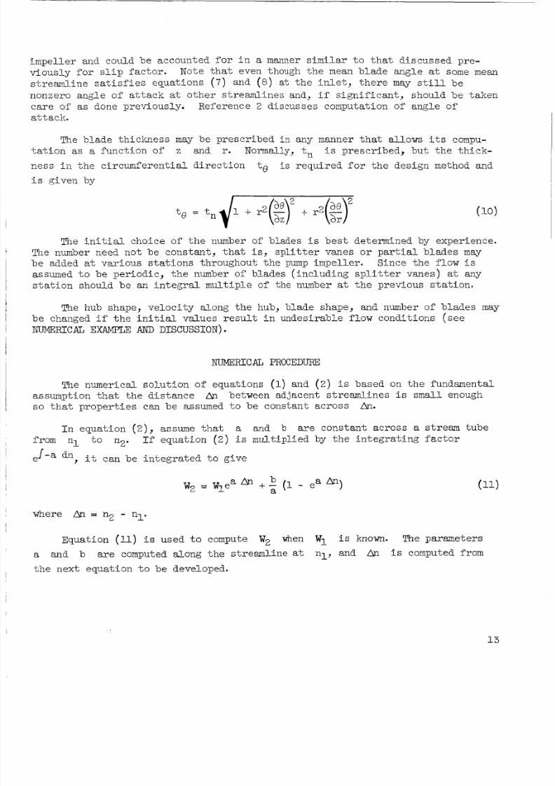
The blade thickness may be prescribed i n any manner that a l lows i t s compu-t a t i o n as a func t i on o f z and r. R o r m a l l y , t, i s presc r i bed, bu t t he t h i ck -
nes s i n t h e c i r cu m f e r e n t ia l d i r e c t i o n te i s r e q u i re d for the design method and
i s given by
to = tn+-qEJqyThe i n i t i a l c ho ic e of the number of blades i s bes-t determined by experience .
The number need not be cons tant , t h a t i s , s p l i t t e r vanes or p a r t i a l b l ades may
be added a t var ious s t a t io ns th roughout th e pump impel l e r . S ince the f low i sassumed t o be per iod ic , t h e number of b l ades ( inc lud ing s p l i t t e r vanes) a t any
s t a t i o n s ho ul d b e a n i n t e g r a l m ul t i p le o f t h e number a t t h e p r e vi ou s s t a t i o n .
The hub shape , v el o ci ty alon g th e hub, bl ade shape, and number o f blades may
be changed i f t h e
NUMERICAIL EXAMPIIF:
i n i t i a l va lue s r e s u l t i n -undes i rab le f low condi t ions ( se e
AND DISCUSSION)
NUMERICAL PROCEDURE
The numerical sol ut io n of eq uat ions (1)and ( 2 ) i s based on t h e fundamental
a s sum pt i on t ha t t he d i s t ance An between adjacent s t reaml ines i s small enough
s o t h a t p ro per t i es can be assumed t o be cons tan t across An.
I n e q ua ti on (Z), assume t h a t a and b a r e cons tan t acros s a stream t ube
dn, it c an b e i n t e g r a t e d t o g i v e
from nl t o n2. I f equat ion ( 2 ) i s m u l ti p li e d by t h e i n t e g r a t i n g f a c t o r
e
where An = nZ - nl.
Equat ion (11) i s used t o compute W, when Wl i s known. The parameters
a and b a re computed along the streamline a t nl, and An i s computed from
th e nex t equa t ion t o be developed .
13
8/8/2019 19630001806_1963001806 (Metodo Numerico de Diseno)
http://slidepdf.com/reader/full/196300018061963001806-metodo-numerico-de-diseno 15/36
Equation (1) can be solv ed by ap plyin g t h e mean-value theorem. F i r s t , con-s i d e r t h e i n t e g r a t io n w ith r e s p ec t t o 8 :
-where im s eva l ua t ed a t some 8. Assume t h a t Rm i s t h e Wm of t h e mean
s u r f a c e S. A t any value of n
where r and t o a re f u n c t i o n s of n. Now equati on (1)can be w r i t t e n as
W,(2~cr - Mte)dn
Assume t h a t Wm(25(r - Mte) i s cons t an t ac ros s An. Then
AQ = Wm(2rrr - Mte)(n2 - nl)
Hence
AQ
Wm ( 2rrr - Mte)=
where
a and b of equa t ion (11).
Wm(2Kr - M t e ) i s eva l ua t ed on t he s t r eam l i ne a t nl, as are t he pa ram e t e r s
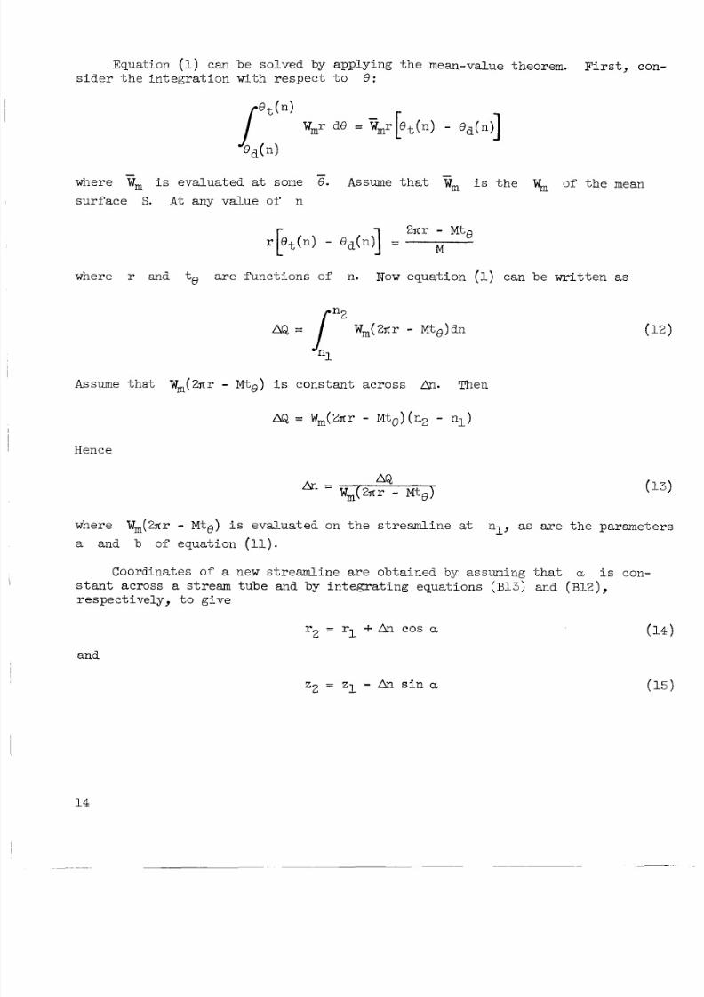
Coordinates of a new streamline are ob ta in ed by assuming ’chat a i s con-
s t a n t a c r o s s a stream t u b e a nd by i n t e g r a t i n g e q u a ti o n s (B13) and ( B 1 2 ) ,
r e s p ec t iv e l y, t o g i v e
and
z2 = z1 - AI i n a
14
8/8/2019 19630001806_1963001806 (Metodo Numerico de Diseno)
http://slidepdf.com/reader/full/196300018061963001806-metodo-numerico-de-diseno 16/36
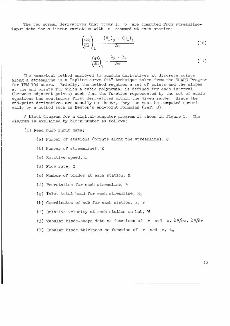
The -two normal de ri va t i ve s t h a t occur i n b are computed from streamline-
i n p u t da ta f o r a l i n e a r v a r i a. t io n w tt h n assumed a t e a c h s t a t i o n :
The numerical zethod employed t o coapdte de ri va t i ve s a t d i s c r e t e p o i n t s
a long a s t r e a m l i n e i s a " sp l i ne cu rve f i t " technique - taken from t h e SI€ARE Program
f o r IB M 704 users . Br i e f ly , t h e method requi res a s e t o f p o i n t s a nd t h e s l o p e s
a t t h e end p o i n t s f o r w hich a cubic polynomia.1 i s d e fi ne d f o r e ac h i n t e r v a l
(between a .d j acent po i n t s ) such t h a t t h e func t ion represen ted by th e s e t of cubic
equat ions has cont inuous f i r s t de r i v a t i v e s w i th i n t h e g i ven r ange . S i nce t h e
end -po i n t de r i va t i ve s a re us ua ll y no t known, the y 'coo must be computed numeri-
c a l l y by a method such as Newton's end-point formulas ( r e f . 8 ) .
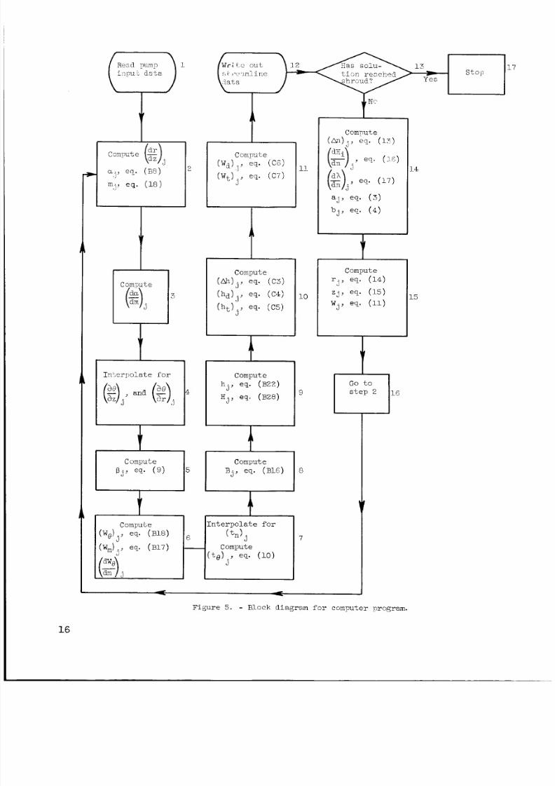
A block d iagram for a digi tal-computer program i s shown i n f i g u r e 5. The
diagram i s explained by block number as fol lows:
(1)Read pump input data:
( a ) Number o f s t a t i o ns (po i n t s a long t he s t r ea m l i n e ) , J
(b ) N-umber of s t reaml ines , K
( e ) Rota .t ive speed , cu
( d ) Flow r a t e , Q
( e ) Number of blades a t each s t a t i on , M
( f ) Pre r o t a t i o n f o r each st r eam li ne , h
(g) I n l e t t o t a l head for each s t reaml ine, Hi
(h) Coordinates of hub f o r each s ta . t ion, z, r
( i)R e l a t i v e v e l o c i t y a t each s ta t ion on hub, W
( j ) Tabular blade-shape da ta as func t ions of r a-?d z, a Q / a z , a0/ar
( k ) Tabu1a.r bla de thi ck ne ss as func t ion of r and z, t n
15
8/8/2019 19630001806_1963001806 (Metodo Numerico de Diseno)
http://slidepdf.com/reader/full/196300018061963001806-metodo-numerico-de-diseno 17/36
i ipuL data
Compute (-
aj, ( B B )L
m,:, eq. ( 1 8 )
\I
Compute
(%) . 3
J
Inseryolate for
and (2).
t
wr;i outL i r , Y ? d i n e t i r > n r e a c k ~ d Stop
I
Comput
hj, eq. ( B 2 2 )
Hj, eq. ( B 2 8 )IComputeB j , eq. ( B 1 6 ) 8
P I
7
15
17
-
Figure 5. - B l o c k diagram f o r computer program.
16
8/8/2019 19630001806_1963001806 (Metodo Numerico de Diseno)
http://slidepdf.com/reader/full/196300018061963001806-metodo-numerico-de-diseno 18/36
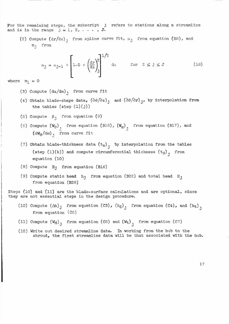
or t h e re ma in in g s t e p s , t h e s u b s c r i p t j r e f er s t o s t a t i o n s a lo ng a s t r e a m l i n e
nd i s i n t h e raDge j = 1, 2, . . . , J.
( 2 ) Compute ( d r / d z )
mJ from
from s p l i n e c ur ve f i t , aj from equat ion (B8), and
ji8j
ml = 0
( 3 ) Compute (da/dm)
(4) Obta in b lade-shape da ta , (a e / az ) j
from curve f i t
and (he/&) ., b y i n t e r p o l a t i o n f r o mJ
t h e tables ( s t e p ( l ) ( j ) )
from equat ion (9)Pj
5 ) Compute
( 6 ) Compute (We) from equation (B18), (W,) from equ atio n (B17), and3 3
(dWe/dm)j from curve f i t
( 7 ) O bta i n b l ade- t h ickness da t a ( t n ) by i n t e rpo l a t i on f rom t h e tablesj
( s t e p (1)k ) ) and compute c i r cum fere n t i a l t h i ckn ess ( t e )
equa t i on (10)
fromj
( 8 ) Compute B j from equation (B16)
( 9 ) Compute s t a t i c head hJ from equat ion (B22) and t o t a l head Hj
from equat ion ( B 2 8 )
(10) and (11) are t h e b l ade - su r face ca l cu l a t i ons and are o p t i o n a l , s i n c e
are n o t e s s e n t i a l s t e p s i n t h e d e si gn pro ced ure.
(10) Compute (hh)j f rom equat io n ( C 3 ) , (ha ) from equat ion (C4), and (h t )3 j
f rom equat ion ( ~ 5 )
(11)Compute (Wa)j
(12 ) Write o u t d e s i r e d s t r e a m l i n e d at a.
from equation (C6) and ( W t ) f rom equat ion (C7)j
In work ing f rom t h e hub t o t h e
shroud, the f i r s t s t r e a m l i n e d a t a w i l l b e t h a t a s s o c i a t e d w i t h th e hub.
1 7
8/8/2019 19630001806_1963001806 (Metodo Numerico de Diseno)
http://slidepdf.com/reader/full/196300018061963001806-metodo-numerico-de-diseno 19/36
Q u a t i t i e s t h a t occur i n t h e ca l cu l a t i on p rocedu re o f p o t e n t i a l i n t e r -
e s t a r e :
(a) Streani l ine coordinates
( b ) R es u l t mt and component ve lo c i t i e s
( e ) Meridiona l s t rea ml in e curva ture
( d ) Blade-curva,ture components
( e ) Angles CL and p
( f ) St a - t i c head and t o t a l head
( 0 " ) B l ad e -s u rf a ce v e l o c i t i e s and s t a t i c head
(h ) C i rcum fe ren ti a l b l ade t h i ckn ess
(13) Test whether or no t t he so l u t i o n has r eached t h e shroud. ( I f t he sh roudi s t he s t a r t i n 2 st re a ml in e , t h e l o g i c i s s t i l l t h e same and t he des i gn
i s f i ni sh ed when t h e hub i s reached; however, i f some intermediate
s t r e a m l i n e i s t h e i n i t i a l one, t h e d e s ig n ha s t o p ro ce ed from t h i s
s t reaml ine t o bo th the hub and the shroud, and th e lo g i c must be
changed s l i gh t l y . )
s t e p ( 1 7 ) ; i f i t has not , go - to s t e p ( 1 4 ) .
I f t he so l u t i o n has r eached t he shroud, go t o
(2) ($from equation (16),1 4 ) Compute (An)j from equa.tion (13),
Yrom equat ion (17), aj from equation ( 3 ) , and b j f rom equat ion ( 4 )
(15) Compute next s t r eam l i ne coo rd i na t e s and ve l oc i t y : r from equa-j
t i o n (14), zj from equabion (15), and Wj rrom equat ion (11)
(li)Return tu s t e p ( 2 )
(17) SLOP
NUMERICAL EXAMPLE AND DISCUSSION
The digi tal-computer program as o u t l i n e d i n t h e p re ce di ng s e e- ti on w a s
a p p l i e d t o a numer ica l example f o r t he purpose o f i l l u s t r a t i n g t he u se o f t h e
method. The fo llo wi ng i s a l i s t of t h e cond i t ions p re sc r i bed :
(1)Number of stations, 26, approximate ly equa l ly spaced wi th d i s t ance a longmer id iona l hub contour
8/8/2019 19630001806_1963001806 (Metodo Numerico de Diseno)
http://slidepdf.com/reader/full/196300018061963001806-metodo-numerico-de-diseno 20/36
(2) Number of streamlines, 40
(3) Rotative speed, u) , 1571 radians/sec
(4)Flow rate, Q, 48 cu ft/sec
(5) Number of blades, M, 4 at each station (no splitter vanes)
(6) Prewhirl, h, 0; inlet total head, Hi, 1304 ft
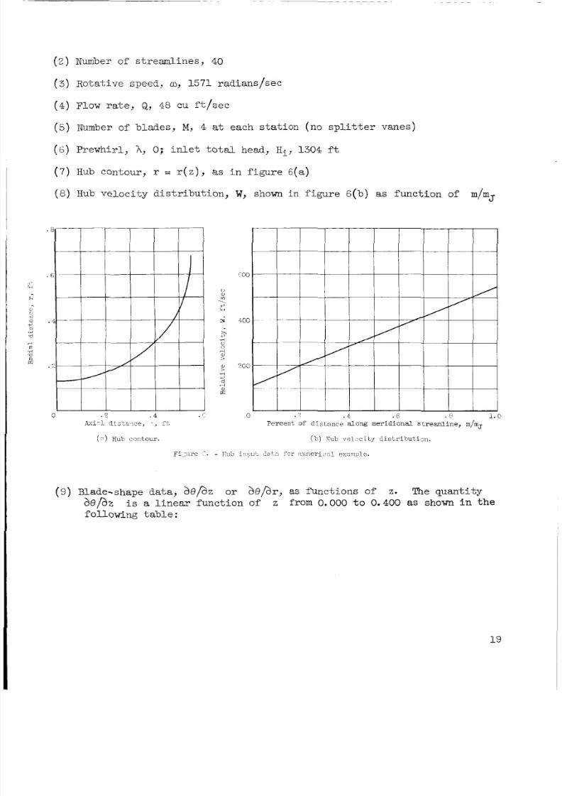
(7) Hub contour, r = r ( z ) , as in figure 6(a)
(8) ub velocity distribution, W, shown in figure G(b) as function of m/mJ
hi-l d i s t n l c e , -', ~
( ? ) Hub contour.
Fi.;u-e ^ .
0 . 4 . E . A 1. '
Percent of distance a long mer id iona l s t reaml ine , m/mJ
(b) Vub \,el city distrihutim.
- F;ub i i i i u i Sa l 3 f o r numeric11 example.
(9) Blade-shape data, &/az or a@/&, as functions of z. The quantity
& / a 2 is a linear function of z from 0.000 to 0.400 as shown in thefollowing table:
19
8/8/2019 19630001806_1963001806 (Metodo Numerico de Diseno)
http://slidepdf.com/reader/full/196300018061963001806-metodo-numerico-de-diseno 21/36
from impellerinlet,
I Z
0.000,050
.150
-250
,350
.390
.395
,400.405
.410
.500
.600
B1 de shapespecific t ion
~
-10.39374-9.09453
-6.49609
-3.89765
-1.29922
-.25984
-.129920
I
ae5
0.0
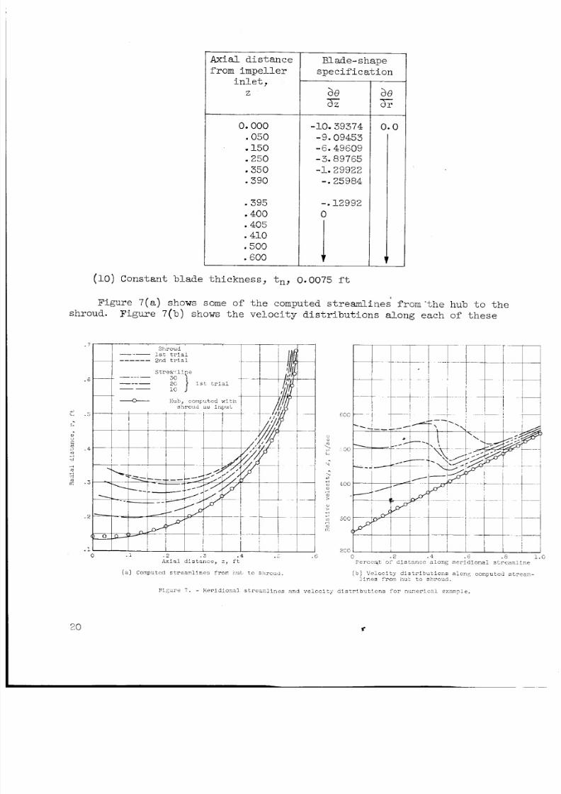
v(10) onstant blade thickness, tn, 0.0075 ft
Figure 7(a) shows some of the computed streamlines. from'the hub to the
shroud. Figure 7(b) shows the velocity distributions along each of these
. 7
. 6
e .5
h
m
c
: .4ro
d
d
4
m
2 .3
.2
.1
. 2 .3 . 4 .I . 6A x i a l d i s t a n c e , z , f t
( a ) C om pu te d s t r e a m l i n e s fror :.ut t o s!n-ouli. ( b ) Velocity d i s t r i b u t i o n s aloni< c o m p u t e d s t r e a n -l i n e s fror : i-.aL to s h r o n d .
?i,:ilre 7 . - K e r id i on n l s t r e a n l i n e s an d v e l o c i t j d i s t r i b u t i o n s for n u n e r i c a i e x a n F l e .
20
8/8/2019 19630001806_1963001806 (Metodo Numerico de Diseno)
http://slidepdf.com/reader/full/196300018061963001806-metodo-numerico-de-diseno 22/36
s t reaml ines .
shape and shroud ve l o c i t y d i s t r i b u t i o n w i t h t h e cond i t i ons p re sc r i bed p re -
F i gu re 7 r e p r e s e n t s t h e f i r s t t r i a l t o o b t a i n a c c e p t a b l e s h ro u d
v i us y.
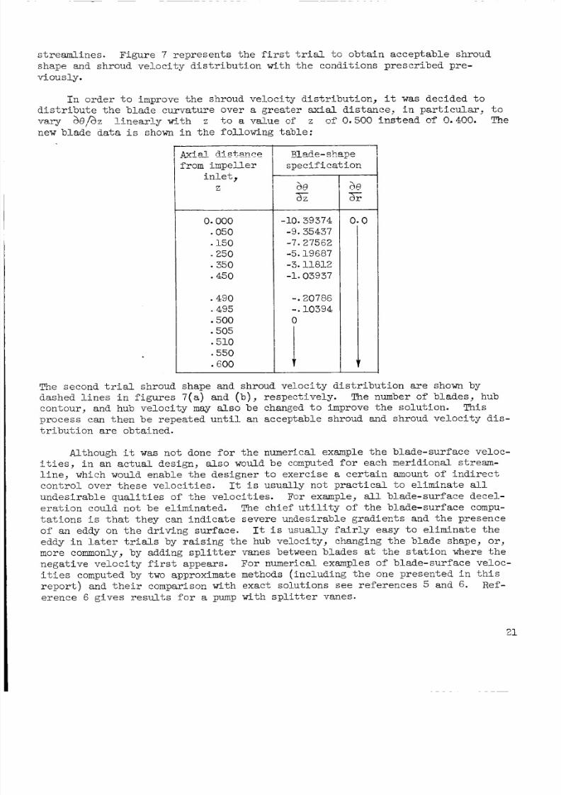
I n o r d e r t o i mp rove t h e s hr ou d v e l o c it y d i s t r i b u t i o n , i t w a s dec ided t o
d i s t r i b u t e t h e bl a de c u rv a tu r e o ve r a g r e a t e r ax ia l d i st a n ce , i n p a r t i c u la r , t ovary aQ,&z l i n e a r l y w5th 2 t.0 a v a k e of z of 0.500 i n s t e a d of 0.400. The
new blade data i s shown i n t h e fo l lowing t ab le :
0.000.050
.150- 250
.350
.450
.490
.495
.500
.505
.510
.550
.600
Elade- shn-pe
s p e c i f i c a t i o n
aeaZ
-10.39374
-9.35437
-7.27562
-5.19687
-3.11812
-1.03937
-.20786-.103940
i
aear
0 3
The second t r i a l shroud shape and shroud ve loc i ty d i s t r ibu t ion are shown byd as he d l i n e s i n f i g u r e s 7 ( a ) a nd ( b ) , r e spec t i ve l y .
contour , and hub velocity may a l s o be changed t o improve t h e so lu t ion .
p roces s can then be repea ted un t i l an acceptab le shroud and shroud ve l oc i ty d i s -
t r i b u t i o n are obtained.
The number of blades, hub
This
Although it w a s not done fo r th e numer ica l example t h e b lade-sur f ace ve loc-
i t i e s , i n a n a c t u a l d es ig n, a ls o would be computed f o r ea ch mer idio nal stream-
l i ne , w hich would enab le t h e des i gne r t o exe rc i se a ce r t a i n amount of i nd i r ec t
c o n t r o l o v er t h e s e v e l o c i t i e s .
u n d e s i r a b l e q u a l i t i e s of t h e v e l o c i t i e s . For example, all b l ade - su r face dece l -
e r a t i o n coul d no t be e l im i na ted . The ch i e f u t i l i t y of t h e blad e-su rfa ce compu-
t a t i o n s i s t h a t t hey can i nd i ca t e s eve re undes i r ab l e g rad ie r , t s and t he p re senceof an eddy on th e dr iv in g sur fac e .
eddy i n l a t e r t r i a l s by ra i s in g th e hub ve loc i ty , changing th e b lade shape , or,more commonly, by adding s p l i t t e r vanes between bl ad es a t t h e s t a t i o n where t h e
n e g a t i v e v e l o c i t y f i r s t appears.
i t i e s computed by two approximate methods ( inc ludin g t h e one presen ted i n t h i s
re po r t ) and t h e i r compari son wi th exac t so lu t ions see r e f e r e n c e s 5 and 6.
e rence 6 g i v e s resul ts for a pump wi th sp l i t t e r vanes.
It i s u s ua l ly n ot p r a c t i c a l t o e l i m i na t e a l l
It i s u s ua l ly f a i r l y e a sy t o e l im i n a te t h e
For numerical examples of blade-surface veloc-
R e f -
8/8/2019 19630001806_1963001806 (Metodo Numerico de Diseno)
http://slidepdf.com/reader/full/196300018061963001806-metodo-numerico-de-diseno 23/36
Although the approximate blade-surface computations also permit indirect
control over the blade-surface static head or pressure, they are unfortunatelyof quite limited value in studying cavitation conditions, as is pointed out in
reference 5. If the time and effort were warranted, however, the method ofreference 5, applied to only one stream tube, might give sufficient informationfor cavitation studies. (In ref. 5, angle of attack was not taken into accountin the approximate calculations so that the off-design case shows worse agreementwith the exact solution at the inlet than would be the case if angle of attackwere included, as suggested in this report.)
As mentioned in the Design Inputs section, the method can also proceed from
Adjustment of conditions on the shroud
shroud to hub by making the sign of
scribing conditions along the shroud.similar to those done to the hub can produce an acceptable hub and hub velocity
distribution. The shroud contour and velocity distribution computed as the first
trial (figs. 7(a) and (b)) were used as input to the program to illustrate start-ing on the shroud and the computed hub and hub velocity distribution, as shownin figures 7(a) and (b), are almost identical with the original prescribed hub
and hub velocities.
An in equation (13) negative and by pre-
In choosing the number of stations for a solution, some care should beexercised to avoid very small spacings especially in regions of large curvaturein order to prevent numerical difficulties that become increasingly worse as the
solution proceeds toward the shroud. The reason is that the spacing gets smallernear the shroud and may become of the same order of magnitude as the error in thenumerical procedures, or the spacing may become negative. In either case, thesolution becomes meaningless in such a region.
A sufiicient numuer of streanbiues ;hodd be ch,;en so that the resultingLM is s m a l l enough to make the assumption of constant a and b in equa-
tion (2) a valid one. The value of An varies with the size of the impellerand can usually be determined in one or two trials. It is probably not worthstarting with less than 10 streamlines. Limited experience indicates that nodifficulties result froIi, having too many streamlines; however, it is a waste of
time to have more than necessary for the degree of accuracy desired.numerical example presented, the results of the solution from the shroud to the
hub indicate that An was chosen s m a l l enough to make the assumption of constanta and b satisfactory.
In the
Lewis Research C3nter
National Aeronautics and Space Administration
Cleveland, Ohio, September 19, 1962
22
8/8/2019 19630001806_1963001806 (Metodo Numerico de Diseno)
http://slidepdf.com/reader/full/196300018061963001806-metodo-numerico-de-diseno 24/36
A
a
b
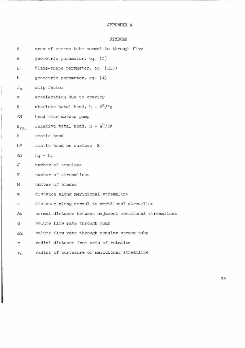
APPENDIX A
SYMBOLS
area of stream tube no-rmal t, o through flow
geome tric parameter, eq. ( 3 )
F l a d e - s h a p p y z T e t e y , eq. ( O ~ C ’-” I
geom etric parameter, eq. (4)
s l i p f a c t o r
a c c e l e r a t i o n d ue t o g r a v i t y
a b s o l u t e t o t a l head , h + Vz/2g
head r i s e across pump
r e l a t i v e t o t a l head, h + W2/2gH r e l
h s t a ti head
h* s t a t i c h ead on s u r f a c e S
Ah hd - ht
J number of sta-t ions
K number of s t r eam l i nes
M number of b l ades
m d i s t an ce a l ong m er id i onal s t r eam l ine
n d i s t an ce a l ong norma l t o m er i d i ona l s t r eam l i ne
An normal d i s t a nc e between ad jacen t mer id iona l s t rea ml i ne s
Q volume flow r a t e through pump
AQ volume flow ra te through annular s t ream tube
r r a d i a l d i s ta n c e from axis of ro t a t i on
r c ra d i us of curva tur e of mer id iona l s t reaml ine
2 3
8/8/2019 19630001806_1963001806 (Metodo Numerico de Diseno)
http://slidepdf.com/reader/full/196300018061963001806-metodo-numerico-de-diseno 25/36
S
t
tn
v
W
Z
a
P
rl
0
ae
A
w
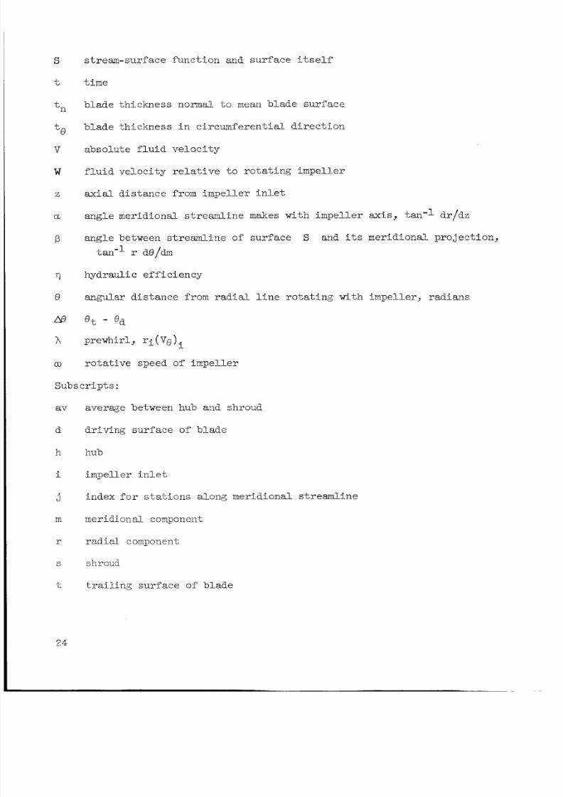
s t r e m - s u r f a c e f u n c t i o n and s u r f a c e i t s e l f
t i m e
blade th ickness normal t o mean blade surface
b lade th ickness i n c i r c u m f e r e n t i a l d i r e c t i o n
a bs ol ut e f l u i d v e l o c i t y
f l u i d v e l o c it y r e l a t i v e t o r o t a t i n g i m pe l le r
a x i a l d i s t a n c e f r o m i m p e l l e r i n l e t
angle meridional s t r ea ml ine makes with i m p e l l e r axis, t a n - l d r / d z
ang le between s t re aml ine of su r face S and i t s mer id iona l p ro jec t ion ,
tan-’ r de/dm
h y d r a u l i c e f f i c i e n c y
a ng ul ar d i s t a n c e f ro m r a d i a l l i n e r o t a t i n g w i th i m p e ll e r, r a di a ns
e t - Qd
prewhirl , r i ( V e )
r o t a t i v e s pe ed o f im p e l l e r
i
S u b s c r i p t s :
av
d
h
i
j
m
r
S
L
24
average between hub and shroud
d r iv in g s u r f a c e o f b l a d e
hub
i m p e l l e r i n l e t
index f o r sta’cions a long meridional s t r eam lin e
meridional component
radial component
shroud
t r a i l i n g s u r f ac e of b l a d e
8/8/2019 19630001806_1963001806 (Metodo Numerico de Diseno)
http://slidepdf.com/reader/full/196300018061963001806-metodo-numerico-de-diseno 26/36
z axial component
0 circumferential component
1 known streamline
2 adjacent unknown streamline
25
8/8/2019 19630001806_1963001806 (Metodo Numerico de Diseno)
http://slidepdf.com/reader/full/196300018061963001806-metodo-numerico-de-diseno 27/36
APPENDIX 13
DERIVATION OF VELOCITY EQUATION
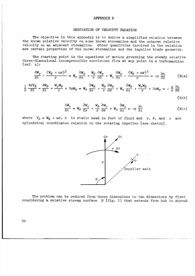
The ob j ec t i ve i n t h i s appendi x i s t o d er iv e a s i m p l i f i e d r e l a t i o n b etween
t h e known r e l a t i v e v e l o c i t y o n some known s t r ea m l i ne and t he unknown r e l a t i v e
v e l o c i t y on an a d j ac e n t st r ea m li ne . O th er q u a n t i t i e s in vo lv ed i n t h e r e l a t i o nare ce r t a i n p r ope r t i e s o f t h e known s t r e a d i n e and t h e i m pe l l e r b l ade geome try.
The s t a r t i n g po i n t i s t h e equa tions of motion govern ing th e s t eady re l a t i v e
three-dimensional incompres sible nonviscous f l o w a t any po in t i n a turbomachine
( r e f . 4):
where Vo t: We + WT, h i s s t a t i c head i n f e e t of f l u i d and r , 0, and z a re
c y l i n d r i c a l c o o rd in a te s r e l a t i v e t o t h e r o t a t i n g i m p e l le r ( s e e s k e tc h ) .
7
r
Z
The problem can be reduced from th r e e dimensions t o two dimensions by f i r s t
S ( f i g . 2) t h a t e x t e n d s from hub t o shroudonsidering a r e l a t i v e stream s u r f a c e
26
8/8/2019 19630001806_1963001806 (Metodo Numerico de Diseno)
http://slidepdf.com/reader/full/196300018061963001806-metodo-numerico-de-diseno 28/36
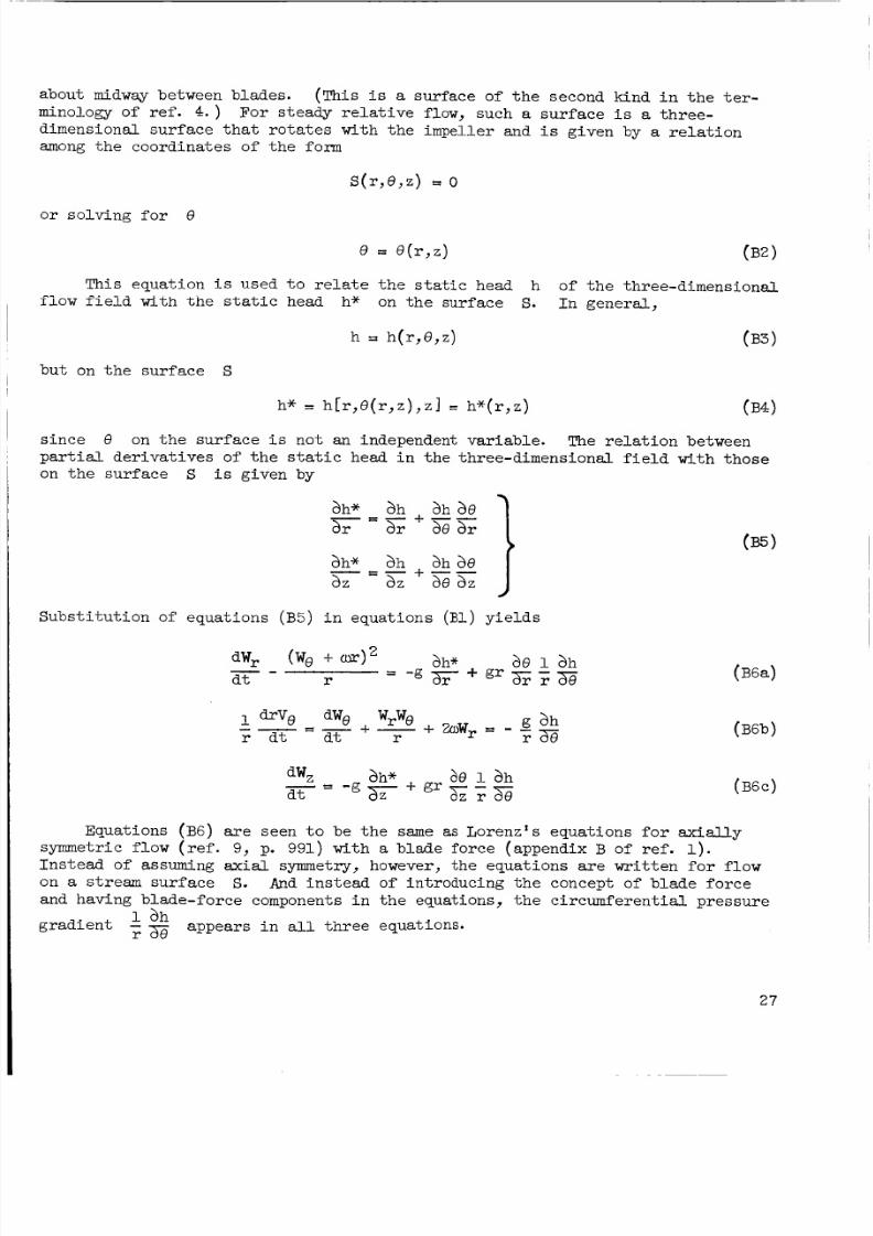
about midway between blades .
inology of ref . 4.)
d im ensi ona l su r f ace t h a t ro t a t e s w i th t h e i m pel l er and i s given by a r e l a t i o n
among th e coor dina tes of th e form
(Thi s i s a s u r fa c e o f t h e s ec on d k in d i n t h e t e r -For steady r e l a t i v e f l o w , such a s u r f a c e i s a t h ree -
or s o l v i n g f o r 8
This equa t ion i s used t o r e l a t e t h e s t a t i c head h o f t h e t h ree -d im ens iona l
f low f i e l d w i t h t h e s t a t i c head h* on th e surf ace S. I n g e ne r al ,
b u t on t h e s u r f a c e S
h* = h [ r , Q ( r , z ) , z ] = h*(r ,z) (B4)
s i n c e 8 on t h e s u r f a c e i s not an independent variable . The r e l a t i on betw een
p a r t i a l d e r i v a ti v e s o f t h e s t a t i c head i n t h e th re e- dim en sio na l f i e l d w it h t ho s e
on t he su r f ace S i s given by
ah* ah a h de- = - + - - JaZ aZ he aZ
Sub s t i t u t i o n o f equa ti ons ( B 5 ) i n e q ua ti on s (Bl) y i e l d s
Equations (B6) w e s ee n t o be t h e same as Lorenz*s equa t ions for a x i a l l y
symmetric flow ( r e f . 9, p. 991) wi th a blade force (appendix B of ref . 1).
Ins t ead of assuming ax ia l symmetry, however, the equa t ions are w r i t te n f o r fl ow
on a stream s u r f a c e S.
and having b lade- forc e components i n the equa tions , t h e c i rc umfe ren t i a l p re ssur e
g r a d i e n t
And in st ea d of int roducing t h e concept of blad e for ce
appea rs i n a l l t h ree equa t ions .ah
- ? z
27
8/8/2019 19630001806_1963001806 (Metodo Numerico de Diseno)
http://slidepdf.com/reader/full/196300018061963001806-metodo-numerico-de-diseno 29/36
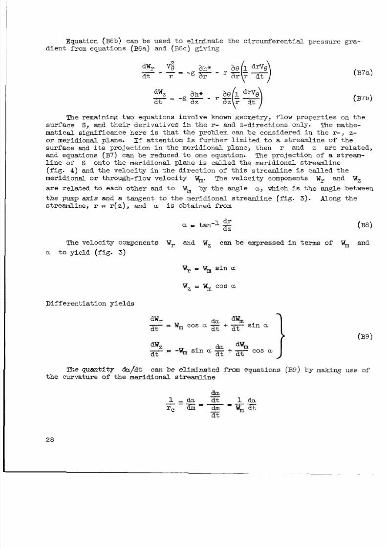
Equation (B6b) can be u sed t o e l i m i na t e t h e c i r c um fe ren t i a l p re s su re g ra -d ien t f rom equat ions ( B 6 a ) and (B6c) giving
The remaining two equations involve known geometry, f low pr op er t i es on th e
s u r f a c e S, and t h e i r d e r i v a ti v e s i n t h e r- and z-d i re ct io ns only.
m a t i c a l s i g n i fi c a n c e h e r e i s t h a t t he p roblem can be cons ide red i n t he r-, z-
o r meridional plane.
surface and i t s p r o j e c t i o n i n t h e m er i d io n a l pl an e, t h e n r and z a r e r e l a te d ,
and equat ions ( B 7 ) can be reduced t o one equat ion.
l i n e o f S( f i g . 4) and t h e v e l o c i t y i n t h e d i r e c t i o n of t h i s s t re a m li n e i s c a l l e d t h e
mer id iona l o r through-f low v e lo c i ty W The velocity components W and Wz
are r e l a t e d t o e ac h o t h e r and t o
t h e pump axis and a t a n ge n t t o t h e m e ri d io n a l s tr e a m l i ne ( f i g . 3).st reaml ine, r e r ( z ) , a n d a i s obtained from
The mathe-
I f a t t e n t i o n i s f u r t h e r l i m i te d t o a s t r eam l i ne o f t h e
The p r o j e c t i o n o f a stream-on t o t he m er i d i ona l p l ane i s c a l l e d t h e m e r id i o na l s t r e a m li n e
Wm by t h e ang l e a , which i s t h e angle be tween
Along the
dra = t an -1
The velocity components Wr and Wz can be expressed i n terms of Wm and
a t o y ie l d ( f ig . 3)
Wr P Wm s i n a
Wz I Wm cos a
D i f f e r e n t i a t i o n y i e l d s
Iwr da dw, s i n aa t a t a tw cos a - + -
cos a JWZ d c ~ dwm- Wm s i n a - -a t a t a t
The qu an ti t y da/dt can be el im ina ted from equat ion s (B9) by making use of
t h e cu rva t u re o f t h e m er id i ona l s t r eam l i ne
d t
28
8/8/2019 19630001806_1963001806 (Metodo Numerico de Diseno)
http://slidepdf.com/reader/full/196300018061963001806-metodo-numerico-de-diseno 30/36
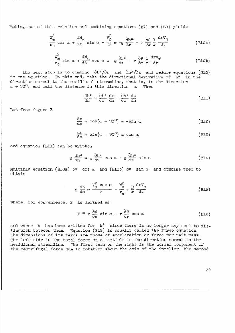
king use of t h i s r e l a t i on and combining equat ion s (B7) and (B9) y i e l d s
( B l O a )
(Blob)
The next s t ep i s t o combine ah*/& and ah */hz and red uce eq ua tio ns (B10)
ah* a0 1 d r b
- g T - r ; S ; t r a tos a =
Wms i n a +-
d t
w2,-T C
t o one equa t ion. To t h i s end, t a k e t h e d i r e c t i o n a l d e r i v a t i v e of h* i n t h e
d i r e c t i o n no rm al t o t h e m e ri d io n al s tr e am l in e , t h a t i s , i n t h e d i r e c t i o n
+ 90°, and call t h e d is t a nc e i n t h i s d i r e c t io n n. Then
But f rom f i gu re 3
dz- cos(a. + 90') 3 - s i n adn
= s i n ( a + 900) t cos adn
and equat ion ( B 1 1 ) can be w r i t t en
dh* - g G c o s a - g ~ s - n ah* ah*
g d n -
Mul t ip ly equa t ion ( B l O a ) by cos a and (Blob) by s i n a and combine them t o
o b t a i n
V~ cos a W drV@m B- - + - -h
g - Idn r rc r d t
where, f o r convenience, B i s de f i ned as
B E r '0 s i n a - r $ cos a
aZ
4)
and where h has b e en w r i t t e n f o r h* s i n ce t h e r e i s no long er any need t o a i s -t inguish between them.
The dimensions of i t s t e rm s a r e those o f acc e l e ra t i on or f o r c e p e r u n i t m a s s .
The l e f t s i d e i s t h e t o t a l f o rc e on a p a r t i c l e i n t h e d i r e c t i o n normal t o t h e
mer id ion a l s t reaml ine . The f i r s t term on t h e r i g h t i s t h e normal component of
t h e c e n t r i f u g a l f o r c e due t o r o t a t i o n a b ou t t h e axis of t h e im pe l l e r , t h e second
Equat ion ( B 1 5 ) i s u s u a l l y c a l l e d t h e f o r c e e q u at io n.
29
8/8/2019 19630001806_1963001806 (Metodo Numerico de Diseno)
http://slidepdf.com/reader/full/196300018061963001806-metodo-numerico-de-diseno 31/36
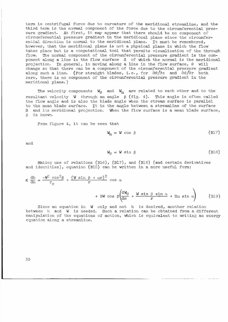
term i s cen t r i fu ga l fo rc e due t o curva tu re of the mer id iona l s t reaml ine , and th e
t h i r d term i s t h e n r m a l component o f t h e f o r c e du e t o t h e c i r c u mP e r e n ti a l p r es -
sure g rad ien t . A t f i r s t , i t ma;y appear that there should be no component ol"
c i r c um f e r e n ti a l p r e s s u r e g r a d i e n t i n t h e m e r id ion a l p l a ne s i n c e t h e c i r c u n f e r -
e n i i a l d i r e c l i o n i s normal t o t he mer id iona l p lane.
however, t h a t t h e m er idio n al p l an e i s n o t a p h y s i c a l p l a ne i n which t h e f l o w
ta k e s p l a c e b u t i s a c om p utat io n al t o o l t h a t p e r m i ts v i s u a l i z a t i o n of t h e t h ro u ghflow. The normal component oT t h e c i r c u m f e r e n t i a l p r e s s u r e g r a d i e n t i s t h e com-ponent along a l i n e i n t h e f lo w su r fa c e S of which t h e normal i s t h e m e r id io n a l
pro jec t ion . In genera l , i n moving a long a l i n e i n t h e f lo w s u rf ac e, 8 w i l l
change s o t h a t t h e r e c an b e a component o f th e c i rcu mfe ren t ia l p ress ure g r ad ie n t
along such a l i n e . (For s t r a i g h t b la de s, i . e . , f o r a @ z an d &/ar b o t h
zero, there i s no component o f t he c i rc umf eren t ia l p ressu re g rad ie n t i n th e
meri.dionaL plane. )
I t must be remembered,
The veloci-ty components We an d Wm a re r e l a t e d t o e ach o t h e r and t o t h e
r e s u l t a n t v e l o c i t y W throuzh an angle p ( f i g . 4 ) . T h is a n g l e i s o f t e n c a l l e d
t he f low ang le and i s a l so th e b la.de ang le when t h e s t ream sur fa ce i s p a r a l l e l
-to the mean blade surface. I t i s the angle between a s t r e a m l i n e o f t h e s u r f a c eS an d i t s mer id iona l p ro jec t ion . When t h e f l o w s u r f a c e i s a mean blade surface,
B i s known.
From f i g u r e 4, i t can be seen tha t
wm = w cos p
an d
Making use of r e l a t i o n s (B16), (B17), an d (BlB) ( an d c e r t a i n d e r i v a t i v e s
and i d e n t i t i e s ) , e qu a ti on (B15) can be wr i t t en i n a more useful form:
dh -Wz cos'p ( W s i n p + w r ) '+ cos cLg z = r
Since an equat ion i n W only and not h i s d e s i r e d , a n o t h er r e l a t i o n
between h and W i s needed. Such a r e l a t i o n c a n be obtained f rom a dift 'erentmani pulati on of th e equa.tions of motion, which i s e q ui v al e nt t o m i - t i n 3 a n e ne rg y
equat ion a long a s t reamline .
30
8/8/2019 19630001806_1963001806 (Metodo Numerico de Diseno)
http://slidepdf.com/reader/full/196300018061963001806-metodo-numerico-de-diseno 32/36
d r d edt '
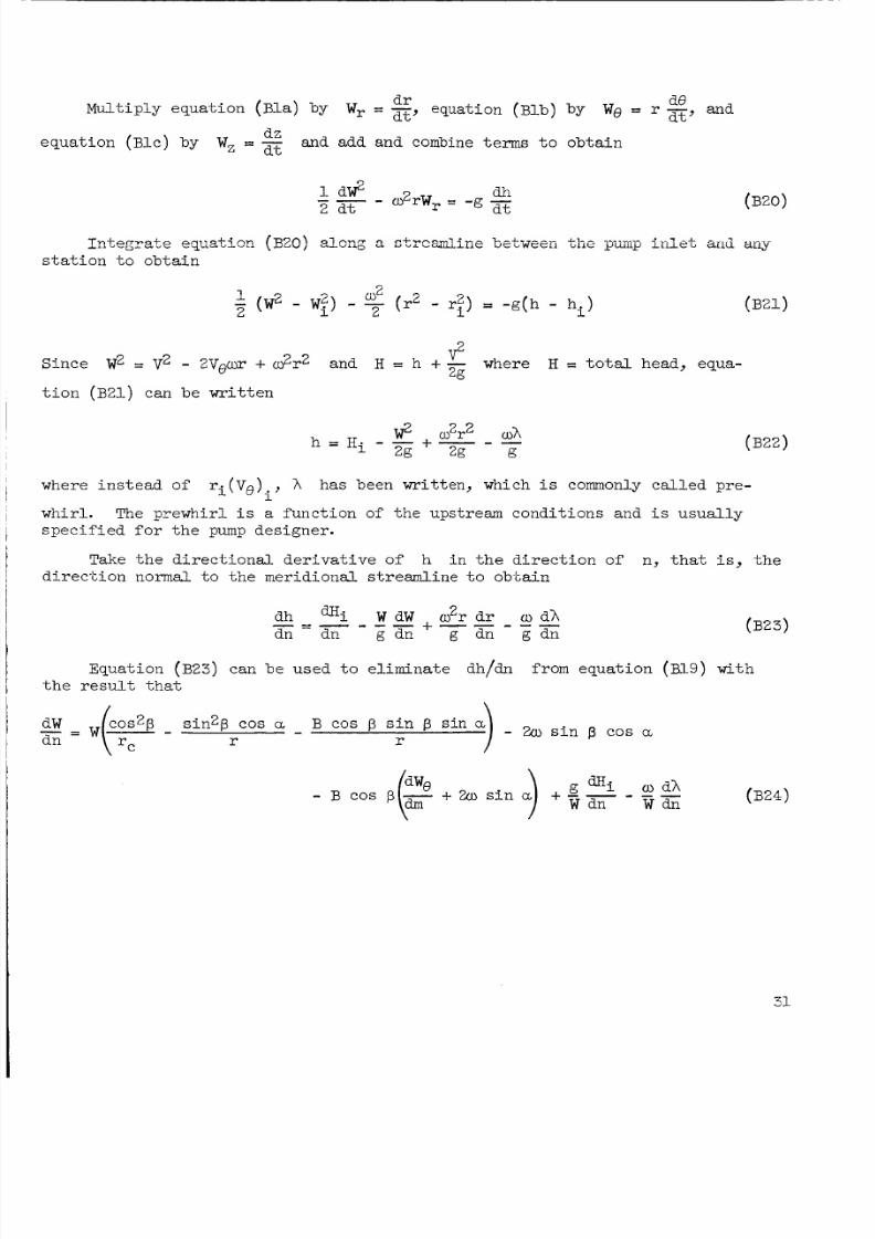
u l t ip ly equat ion ( B l a ) by Wr =- equation ( B l b ) by We = r dt' and
equa t ion (Blc ) by W, c E and add and combine terms t o o bt ai n
where H = t o t a l head, equa-2
Since W2 = V2 - 2 V e c ~ r+ d r 2 and H = h +-2i5
t ion (B21) canbe
w r i t t e n
where i n s t e a d of
wh irl . The pre whi rl i s a f u n c t i o n of th e upstream condi t ions and i s u s u a l l y
s p e c i f i e d f o r t h e pump designer .
r i ( V o ) , A has been writ t en, which i s commonly c a l l e d pre-i
Take t h e d i r e c t i o n a l der iva t ive of h i n t h e d i r e c t i o n of n , t h a t i s , t h e
d i r e c t i o n no rm al t o t h e m e r id io n al s t re a m li n e t o o b t a i n
dh W dW 0% d r w dh-e---- + - - - - -dn dn g dn g dn g dn
Equat ion (B23) can be used t o e l i mi na te dh/dn from equation (B19) with
t h e r e s u l t t h a t
s in20 cos a B cos p s i n p s i n- - ZW s i n p cos ar r
31
8/8/2019 19630001806_1963001806 (Metodo Numerico de Diseno)
http://slidepdf.com/reader/full/196300018061963001806-metodo-numerico-de-diseno 33/36
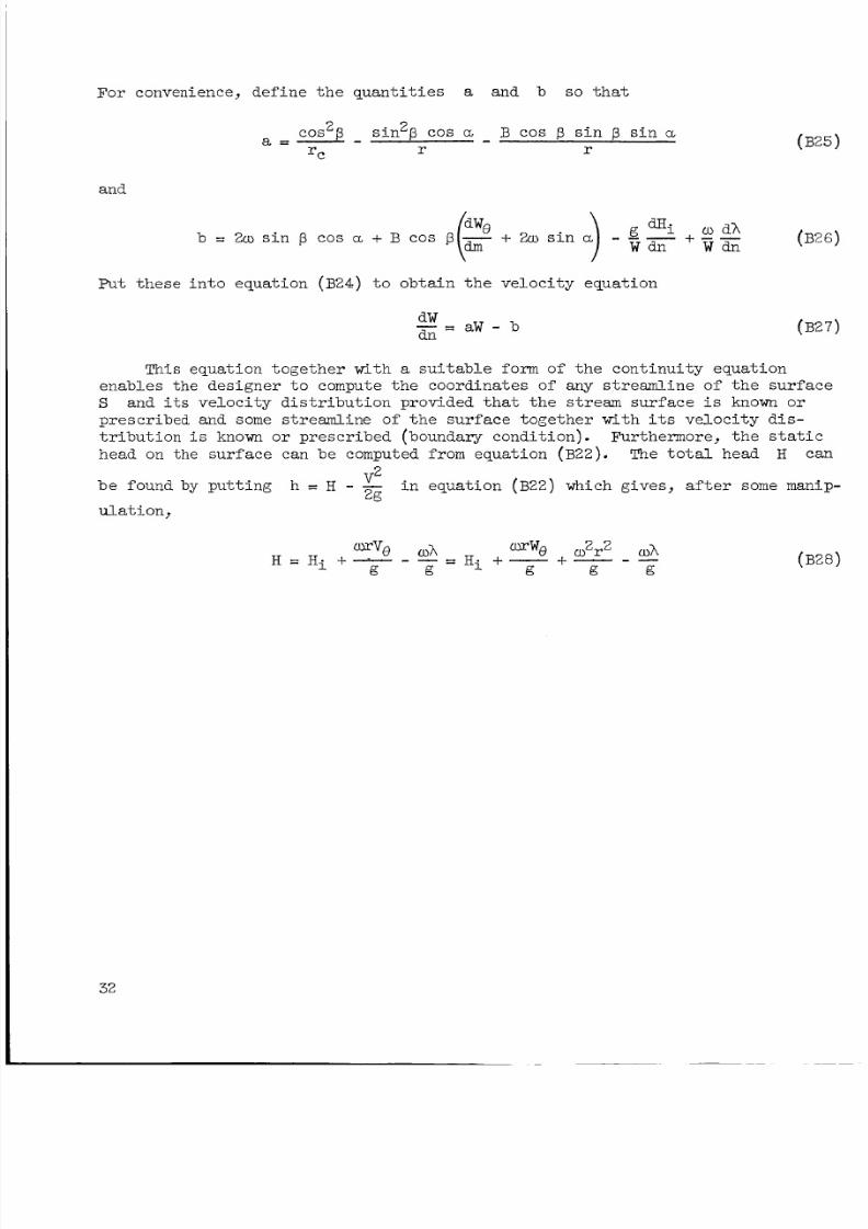
For convenience , de f in e th e quan t i t i e s a and b so t h a t
cos2p s i n p cos a B cos p s i n p s i n aa=-- -r r
T C
and
P u t t h e s e i n to e q u a t io n (B24) t o o b t a in t h e v e lo c i t y e q u at i on
- -- a W - b
This equa t ion toge ther wi th a s u i t a b l e fo rm o f t h e c o n t i n u i t y e q u a t i o n
enab les the des ig ner t o compute th e coord ina tes of any s t r e a m l in e o f t h e s u r f a c e
S and i t s v e l o c i t y d i s t r i b u t i o n p r ov id ed t h a t t h e stream s u r f a c e i s known or
presc r ibed and some s t reaml ine o f t h e su r face t oge th er wi th i t s v e l o c i t y d i s -
t r i b u t i o n i s known o r prescr ibed (boundary condi t ion) .
head on the surface can be computed from equation (B22). The t o t a l head H can
F ur th er mo re , t h e s t a t i c
h
b e found by p ut t i ng h = H - -' n equa tio n (B22) which giv es, a f t e r some manip-2g
ula-t n,
32
8/8/2019 19630001806_1963001806 (Metodo Numerico de Diseno)
http://slidepdf.com/reader/full/196300018061963001806-metodo-numerico-de-diseno 34/36
APPENDIX c
EQUATION FOR BLADE SURFACE VELOCITY AND HEAD RISE
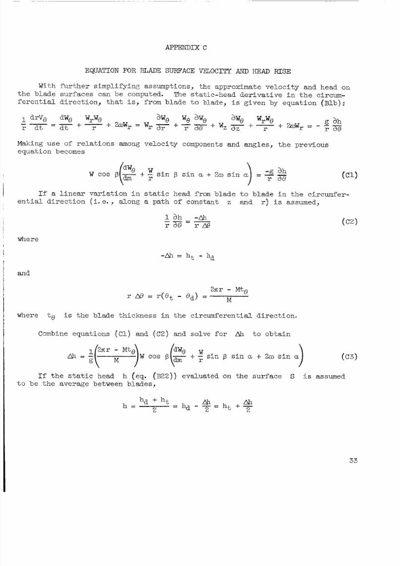
With f ur th e r s impl i fying assumptions , the approximate vel oc i ty and head o nt h e blade sur fa ce s can be computed. The s t a t i c - h e a d d e r iv a t i v e i n the c i rcum-
ferenCYial d i rec t io n, t h a t i s , f rom b lade t o b lade , i s given by equat i on (Blb) :
a w ~ W r W e + ZWW, = - r -ahdrVe dWe WrWe awe We aw e
r d t - d t +- r rilcuw, = W r + + Wz + -- - -
use of r e l a t i o n s among ve lo ci ty components and ang les, t h e previo us
equation becomes
w cos p ( 2 + s i n p s i n a t 2w s i n a) = -g ;sehr
I f a l i n e a r v a ri a ti o n i n s t a t i c head from blade to b la d e i n t h e c i rc um f er -
e n t i a l d i r e ct i o n ( i . e . , a lo ng a pat h of consta nt z and r ) i s assumed,
1 a h -Ah
where
and
where to i s t h e b l a d e t h i c k n e ss i n t h e c i rc u m fe r en t ia l d i r e c t i o n .
Combine equations ( C l ) and (C2) and solve f o r Ah to o b ta in
r
If th e s t a t i c head h (eq. (B22) ) eva lua ted on th e su r face S i s assumed
t o be th e average between b lades ,
ohh t + -
2h d - - rh
2 2
hd + h th =
33
8/8/2019 19630001806_1963001806 (Metodo Numerico de Diseno)
http://slidepdf.com/reader/full/196300018061963001806-metodo-numerico-de-diseno 35/36
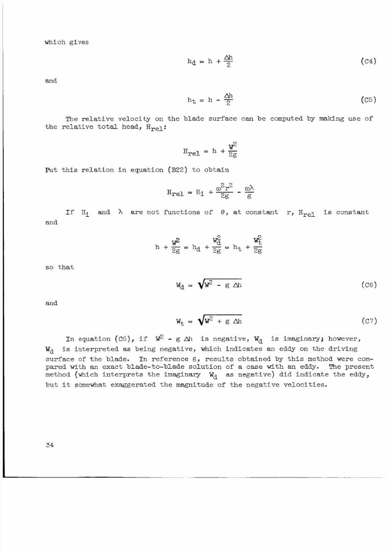
which gives
and
ab2
d c h + -
h t = h - -Ah2
The re la t i ve ve lo ci ty on the bl ade sur fac e can be computed by making us e of
t h e r e l a t i v e t o t a l head, Hrel :
P u t t h i s r e l a t i o n i n e q ua ti on (B22) t o o b t a i n
If Hi and A are n o t f u n c t i o n s of 8 , a t cons tan t r , Hrel i s cons tan t
and
s o t h a t
and
I n equation ( C 6 ) , i f WZ - g i s neg ati ve, wd i s imaginary; however,
wd i s i n t e r p r e t e d as be ing negat ive , which in d i ca te s an eddy on th e d r i v i ng
s u r f a c e o f t h e b la de . I n r e f e r e n c e 6, r e s u l t s obta ined by t h i s method were com-pared with an exact b lade- to-blade so lu t i on of a c a s e w i th a n eddy. The p r e se n t
method (which in te rp re ts t h e imaginary
but i t somewhat exaggerated t h e magnitude of t h e neg at ive v el oc i t ie s .
wd as n e g a t iv e ) d id i n d i c a t e t h e eddy,
34
8/8/2019 19630001806_1963001806 (Metodo Numerico de Diseno)
http://slidepdf.com/reader/full/196300018061963001806-metodo-numerico-de-diseno 36/36
1. Hamrick, Joseph T., Ginsburg, Ambrose, and Osborn, Walter M. : Method of
Analysis for Compressible Flow Through Mixed-Flow Centrifugal Impellers ofArbitrary Design. NACA Rep. 1082, 1952. (Supersedes NACA TN 2165.
2. Smith, Kenneth J., and Hamrick, Joseph T.: A Rapid Approximate Method forthe Design of Hub Shroud Profiles Of Centrifugal Impellers of Given Blade
Shape. NACA TN 3399, 1955.
3. Osborn, Walter M., Smith, Kenneth J., and Hamrick, Joseph T.: Design and Test
of Mixed-Flow Impellers. VI11 - Comparison of E -qe r i rnen t d g e s 7 L t s fcrThree Impellers with Shroud Redesigned by Rapid Approximate Method.RM E56L07, 1957.
NACA
4. Wu, Chung-Hua: A General Theory of Three-Dimensional Flow in Subsonic andSupersonic Turbomachines of Axial-, Radial-, and Mixed-Flow Types. NACATN 2604, 1952.
5. Kramer, James J., Stockman, Norbert O., and Bean, Ralph 5. : Nonviscous Flow
%rough a Pump Impeller on a Blade-to-Blade Surface of Revolution. NASATN D-1108, 1962.
6. Kramer, James J., Stockman, Norbert O., and Bean, Ralph J. : Incompressible
Nonviscous Blade-to-Blade Flow Through a Pump Rotor with Splitter Vanes.NASA TN D-1186, 1962.
7. Stanitz, John D., and Prian, Vasily D. : A Rapid Approximate Method forDetermining Velocity Distribution on Impeller Blades of Centrifugal Com-pressors. NACA TN 2421, 1951.
. Scarborough, James B.: Numerical Mathematical Analysis. The Johns Hopkins
Press, 1958.
. Stodola, A. : Steam and Gas Turbines. Vol. 11. McGraw-Hill Book Co., Inc.,
1927. (Reprinted, Peter Smith (New York), 1945.