2. Creating and Saving Datasets - 国際大学 · . u c:\stata\data\cancer if area==1, clear nol The first command loads first 10 observations from the dataset, while the second reads

$Page 1: 2. Creating and Saving Datasets - 国際大学 · . u c:\stata\data\cancer if area==1, clear nol The first command loads first 10 observations from the dataset, while the second reads$
© 2003-Present Hun Myoung Park (2/23/2013) Stata Datasets: 1

http://www.sonsoo.org

2. Creating and Saving Datasets This chapter discusses how to create, save, and load a dataset, and how to store what you have done to a log file. 2.1. Creating a Dataset Using Data Editor (.edit) Before conducting analyses, you need to get a dataset in memory. You may create a dataset by typing in data, loading an existing Stata data file (see the next section), or importing one from other types of data files (see Chapter 8). This section addresses the first case. Suppose you wish to create a dataset of the data listed as follow.

State Cigar Bladder Lung Kidney Leukemia Area AK 30.34 3.46 25.88 4.32 4.90 3 AL 18.20 2.90 17.05 1.59 6.15 3 AZ 25.82 3.52 19.80 2.75 6.61 4 AR 18.24 2.99 15.98 2.02 6.94 3 CA 28.60 4.46 22.07 2.66 7.06 4

You need to open Stata Editor window by choosing DATAData Editor, choosing WINDOWData Editor (Ctrl + 7), or executing the .edit command. . edit

Editor window looks like a spreadsheet such as Microsoft Excel and Quattro Pro. You may see the highlighted cell called cell pointer at the first column and first row. First, type in “AK” and hit ENTER. You may find that “var1” appears at the top of the first column and “1” in the far-left of the first row. Column corresponds to variables, while row represents observations; so “var1” is the name of

the first variable and “1” is the serial number of the first observation. Now the second row and first column is highlighted. Type in “AL” and hit ENTER again. Cell pointer is now at the third row. You can see the “2” in the far-left of the second row. Repeat the same process until “CA.”



Now, locate the cell pointer to the second column and first row using arrow keys or mouse. Then, type in “30.34” and hit ENTER. Similarly, “var2” occurs at the top of the second column and cell pointer is located at the second row of the column. You can see dot (.) in the second through fifth row of the second column. The dot indicates a missing value of a numeric variable. Keep typing in the data all the way though the end. You may have seven variables from var1 through var7, which are automatically assigned by Stata regardless of users’ preferences.

You may want to change the variable names. Double-click the first column to pop up the Stata Variable Information dialog box. Provide a variable name “state” instead of “var1”, and then click OK. Again double-click other columns to change corresponding variable names. After making sure no error in data entry, close the Stata Editor window by choosing FILEExit (Alt + F4) or clicking icon at the right top of the Editor window. Do not worry about losing data since the current dataset

remains in the memory. Note that you cannot save the data before closing the Editor window. Now you are ready to store the data into a secondary storage unit (e.g., harddisk, floppy disk, zip disk, flash memory). Keep in mind that any change in the current dataset is not

permanently stored until you save it. Choose FILESave (Ctrl + S) or clicking icon to save the data. Then, choose the directory and provide the file name you prefer in the dialog box. Or you may just execute the .save command as follow. . save c:\stata\data\cancer.dta file C:\stata\data\cancer.dta saved

Note that you can omit the default extension .dta of Stata data files. Stata reports that the file is saved at the right below the .save command. Since Stata can handle only one dataset at a time, you may need to remove a current dataset out of memory in order to use other datasets. The .clear command eliminates all the variables and observations in the memory. . clear

You may not see anything in the Variables window after the .clear command executed. 2.2. Data Input from Keyboard (.input) 2.3. Loading a dataset (.use)



In order to open a Stata data file, you may choose FILEOpen (Ctrl + O) or clicking icon. Then, locate the right directory and specify a file name. Alternatively, you may use the .use (or . u) command as follow. . use c:\stata\data\cancer.dta

You can see the list of variables of the dataset cancer.dta in the Variables window. Note that the .dta extension, the default extension, can be omitted. If a current dataset is changed, but you may still want to discard changes and load a new dataset, you need to use the clear option at the end of the .use command. The comma is used to separate a command and its options. But do not be confused with the .clear command and the clear option. . use c:\stata\data\cancer, clear

In some case, you may wish to prevent labels of a dataset from being loaded in the memory. The nolabel (or nol) option is the case. . use c:\stata\data\cancer, clear nolabel

If you may want only subset of a dataset loaded, specify variables and/or observations to be read. This is an efficient and safe way of listing observations especially when you have a huge dataset. . use state cigar using c:\stata\data\cancer, clear nol

Note that you cannot omit the using subcommand when variable names are listed. In addition, use the in qualifier to limit the range of observations and if qualifier to select observations that satisfy the condition. Note that “u” is abbreviation of the .use. . use c:\stata\data\cancer in 1/10, clear . u c:\stata\data\cancer if area==1, clear nol

The first command loads first 10 observations from the dataset, while the second reads only those observations whose area is coded as 1. Note that the equal relational operator is not =, but ==. Following example combines three ways of specifying subsets of a data. . u state cigar using c:\stata\data\cancer in 1/10 if cigar < 20, nol

Stata’s Internet feature allows users to load a dataset from web pages through TCP/IP protocol. Just provide the URL after the .use command. You may also use the in and if qualifiers to select the subset of a dataset. The second command reads variable cigar from 1st through 10th observation from the dataset smoking. . use http://www.iu.edu/~statmath/stat/all/ttest/smoking.dta, clear . u cigar using http://www.iu.edu/~statmath/stat/all/ttest/smoking in l/10, clear

Alternatively, you may use the .webuse command to load a dataset over the web. First, you need to check the URL currently set using the .webuse query command. The default URL is http://www.stata-press.com/r8/.



. webuse query (prefix now "http://www.stata‐press.com/data/r8")

Now, let us change the URL using the .webuse set command and load the dataset from there.. . webuse set http://www.iu.edu/~statmath/stat/all/ttest . webuse smoking, clear

If you want to load example datasets shipped with Stata, execute the .sysuse command. Let us see which Stata files are available by running .sysuse dir command, which and then load one of the datasets. . sysuse dir . sysuse auto.dta

You may feel like using the .use command. However, the command does not work; you should use the .sysuse command to Stata example datasets. 2.4. Saving a data set (.save and .saveold)

In order to save the current dataset, choose FILESave (Ctrl + S) or clicking icon. Or you may use the .save (or .sa) command whose usage is quite similar to that of the .use command. Consider the following examples. . save c:\stata\data\cancer.dta . save, replace . save c:\stata\data\cancer, replace . save c:\stata\data\cancer, replace nolabel

To resave the current dataset, you may omit the file name (see the second command). Note that the replace option overwrites an existing file and the nolabel option omits the label from the saved dataset. For the sake of compatibility, you may need to save a dataset in old format (i.e., Stata 7.0). Choose FILESave As (Shift + Ctrl + S) and select Stata 7 Data (*.dta) from the dialog box. Then, specify the directory and file name you prefer. Alternatively, you may use the .saveold command as follow. . saveold c:\stata\data\newcancer

If you have a huge dataset, you may compress it to reduce its size. The .compress command reduces the amount of memory used by a dataset by changing variable types. For example, double type may be changed to float, which may be reduced to int or byte. . compress . save c:\stata\data\small_cancer



3. Navigating (Exploring) Viewing a Dataset This chapter addresses viewing datasets, listing observations, and labeling. 3.1 Viewing Information of a Dataset (.describe) The .describe (or .d) command shows information of the current dataset. . describe Contains data from http://mypage.iu.edu/~kucc625/documents/cancer.dta obs: 44 vars: 7 size: 2,640 (99.9% of memory free) ‐‐‐‐‐‐‐‐‐‐‐‐‐‐‐‐‐‐‐‐‐‐‐‐‐‐‐‐‐‐‐‐‐‐‐‐‐‐‐‐‐‐‐‐‐‐‐‐‐‐‐‐‐‐‐‐‐‐‐‐‐‐‐‐‐‐‐‐‐‐‐‐‐‐‐‐‐ storage display value variable name type format label variable label ‐‐‐‐‐‐‐‐‐‐‐‐‐‐‐‐‐‐‐‐‐‐‐‐‐‐‐‐‐‐‐‐‐‐‐‐‐‐‐‐‐‐‐‐‐‐‐‐‐‐‐‐‐‐‐‐‐‐‐‐‐‐‐‐‐‐‐‐‐‐‐‐‐‐‐‐‐ state str8 %8s cigar double %10.0g bladder double %10.0g lung double %10.0g kidney double %10.0g leukemi double %10.0g area double %10.0g ‐‐‐‐‐‐‐‐‐‐‐‐‐‐‐‐‐‐‐‐‐‐‐‐‐‐‐‐‐‐‐‐‐‐‐‐‐‐‐‐‐‐‐‐‐‐‐‐‐‐‐‐‐‐‐‐‐‐‐‐‐‐‐‐‐‐‐‐‐‐‐‐‐‐‐‐‐ Sorted by: Note: dataset has changed since last saved

The results describe where the dataset comes from, how many observations and variables are in the dataset, what kinds of data types variables have, and so on. You may specify variables to be listed. . d state cigar, detail

If you want to know information of a particular dataset, provide the data file name with full path as follow. In this case, the current dataset remains unchanged. . d using c:\stata\data\open_system.dta, short

Note that the short option suppresses specific information of each variable. You may want to see summary statistics (e.g., mean and standard deviations) of variables in the current dataset. Use the .summarize (or .sum) command. The separator(7) option puts a separate line every seven observations; its default is five. . summarize, separator(7)

Variable | Obs Mean Std. Dev. Min Max ‐‐‐‐‐‐‐‐‐‐‐‐‐+‐‐‐‐‐‐‐‐‐‐‐‐‐‐‐‐‐‐‐‐‐‐‐‐‐‐‐‐‐‐‐‐‐‐‐‐‐‐‐‐‐‐‐‐‐‐‐‐‐‐‐‐‐‐‐‐ state | 0 cigar | 44 24.91409 5.573286 14 42.4 bladder | 44 4.121136 .9649249 2.86 6.54 lung | 44 19.65318 4.228122 12.01 27.27 kidney | 44 2.794545 .5190799 1.59 4.32 leukemi | 44 6.829773 .6382589 4.9 8.28 area | 44 2.568182 1.020664 1 4



3.2 Summary Statistics (.inspect) Like the .codebook, the .inspect command is useful when you wan to keep summary statistics of variables for the future use. . inspect smoke smoke: Number of Observations -------- ------------------------------ Total Integers Nonintegers | # # Negative - - - | # # Zero 22 22 - | # # Positive 22 22 - | # # ----- ----- ----- | # # Total 44 44 - | # # Missing - +---------------------- ----- 0 1 44 (2 unique values)

3.3 Browsing (.browse) The easiest way of taking a look the current dataset is browsing. Choose DATA”Data Browser (read-only editor)” or execute the .browse (or .br) command. The spreadsheet-like interface provides a visual way of viewing observations in the current dataset. However, if your dataset is large enough, browsing may not be a good solution. The .browse is the exactly the same as the .edit except that the former does not allow any change in the dataset. . browse

The .list (or .l) command lists the observations of the current dataset. . list +---------------------------------------------------------------------------+ | state cigar bladder lung kidney leukemia area smoke west | |---------------------------------------------------------------------------| 1. | AK 30.34 3.46 25.88 4.32 4.9 3 1 1 | 2. | AL 18.2 2.9 17.05 1.59 6.15 3 0 1 | 3. | AZ 25.82 3.52 19.8 2.75 6.61 4 1 1 | 4. | AR 18.24 2.99 15.98 2.02 6.94 3 0 1 | 5. | CA 28.6 4.46 22.07 2.66 7.06 4 1 1 | |---------------------------------------------------------------------------| 6. | CT 31.1 5.11 22.83 3.35 7.2 1 1 0 | 7. | DE 33.6 4.78 24.55 3.36 6.45 3 1 1 | 8. | DC 40.46 5.6 27.27 3.13 7.08 3 1 1 | 9. | FL 28.27 4.46 23.57 2.41 6.07 3 1 1 | 10. | ID 20.1 3.08 13.58 2.46 6.62 4 0 1 | …

If observations are more than one page, Stata will list the first page and pause. The “—more—“ at the left bottom indicates that there are more observations to be listed. You may hit ENTER to see one next observation and SPACE to list one next page. If you want to stop listing, press Ctrl+Break. 3.4 Listing Variables and Observations (.list)



If a dataset has many variables and observations, the result of the .list may be messy. You may wish to take a look at some variables or observations rather than all of them. Following examples specify the variables to be listed using wildcards . list state cigar bladder . list state‐lung; . l state l* +‐‐‐‐‐‐‐‐‐‐‐‐‐‐‐‐‐‐‐‐‐‐‐‐‐+ | state lung leukemi | |‐‐‐‐‐‐‐‐‐‐‐‐‐‐‐‐‐‐‐‐‐‐‐‐‐| 1. | AK 25.88 4.9 | 2. | AL 17.05 6.15 | 3. | AZ 19.8 6.61 | 4. | AR 15.98 6.94 | 5. | CA 22.07 7.06 | |‐‐‐‐‐‐‐‐‐‐‐‐‐‐‐‐‐‐‐‐‐‐‐‐‐| 6. | CT 22.83 7.2 | 7. | DE 24.55 6.45 | 8. | DC 27.27 7.08 | 9. | FL 23.57 6.07 | 10. | ID 13.58 6.62 | |‐‐‐‐‐‐‐‐‐‐‐‐‐‐‐‐‐‐‐‐‐‐‐‐‐| 11. | IL 22.8 7.27 | 12. | IN 20.3 7 | 13. | IO 16.59 7.69 | 14. | KS 16.84 7.42 | ‐‐more‐‐

Note that state-lung includes cigar and bladder located between state and lung. “l*” indicates all the variables beginning with “l.” The in and if qualifiers are commonly used to specify observations to be listed. See Chapter 2.8 for the details. First, consider the following examples of the in qualifier. . list in 10/15 . l state k* in 10 . l state cigar lung in 15/‐1 . l state ?i* in ‐5/l +‐‐‐‐‐‐‐‐‐‐‐‐‐‐‐‐‐‐‐‐‐‐‐‐+ | state cigar kidney | |‐‐‐‐‐‐‐‐‐‐‐‐‐‐‐‐‐‐‐‐‐‐‐‐| 40. | VT 25.89 3.17 | 41. | WA 21.17 2.78 | 42. | WI 21.25 2.34 | 43. | WV 22.86 3.28 | 44. | WY 28.04 2.66 | +‐‐‐‐‐‐‐‐‐‐‐‐‐‐‐‐‐‐‐‐‐‐‐‐+

The first command lists all the variables of observation 10 through 15. The second command displays the values of state and kidney of 10th observation. The third lists state, cigar, and lung of observation 15 through the last one. The last command shows state, cigar, and kidney of the last five observations since “?i*” reads any character, i, and any characters. Note that “-5” refers to the fifth observation from the last and “-1” or “l” indicates the last observation. Following examples select observations using the if qualifier. Be careful not to use wildcards (e.g., * and ?) in the if qualifier. . list if area==1



. list if state=="IN"

. l state cigar if missing(cigar)

. l state cigar bladder if (area==2) & (cigar <=20)

. l state cigar lung in 5/25 if (area==4) | (lung >= 30) +‐‐‐‐‐‐‐‐‐‐‐‐‐‐‐‐‐‐‐‐‐‐‐+ | state cigar lung | |‐‐‐‐‐‐‐‐‐‐‐‐‐‐‐‐‐‐‐‐‐‐‐| 5. | CA 28.6 22.07 | 10. | ID 20.1 13.58 | 24. | MT 23.75 19.5 | +‐‐‐‐‐‐‐‐‐‐‐‐‐‐‐‐‐‐‐‐‐‐‐+

The first command lists observations whose area is coded as 1. The second shows that a string variable requires enclosing a string with double quotation marks. The third selects observations whose value of cigar is missing. The fourth lists observations whose area is 2 and cigar is less than or equal to 20. The last example shows how the in and if qualifiers are used at the same time. Note that & and | are respectively “and” and “or” logical operators. The order of the in and if does not matter. Among useful options are noobs, divider, separator(#), string(#), and nolabel. The noobs suppresses observation numbers listed. The divider and separator(#) respectively put dividers of column and separate lines of row. The string(#) truncates a long string so that only first # characters are listed. The nolabel suppresses the value labels and shows the original values. . list state cigar l*, nolabel string(3) . l state cigar kidney in 1/6, noobs divider separator(2) +‐‐‐‐‐‐‐‐‐‐‐‐‐‐‐‐‐‐‐‐‐‐‐‐+ | state | cigar | kidney | |‐‐‐‐‐‐‐+‐‐‐‐‐‐‐+‐‐‐‐‐‐‐‐| | AK | 30.34 | 4.32 | | AL | 18.2 | 1.59 | |‐‐‐‐‐‐‐+‐‐‐‐‐‐‐+‐‐‐‐‐‐‐‐| | AZ | 25.82 | 2.75 | | AR | 18.24 | 2.02 | |‐‐‐‐‐‐‐+‐‐‐‐‐‐‐+‐‐‐‐‐‐‐‐| | CA | 28.6 | 2.66 | | CT | 31.1 | 3.35 | +‐‐‐‐‐‐‐‐‐‐‐‐‐‐‐‐‐‐‐‐‐‐‐‐+

3.5 Counting Observations (.count) This command counts the number of observations that meet the condition specified. . count if cigar > 20 38

3.6 Formatting (.format) The .format command specifies the format of variables to be displayed. But this command does not affect actual values of variables. When a variable is copied, its format is also copied. You may check the current display format of each variable by execute .describe command, which shows variable names, types, formats, and labels. . describe



In general, a format begins with % that is followed by a number (the total number of digits), period, a number (the number of digits below the decimal point), and letters indicating types of format. Let us put a comma in variable in order to make numbers more readable. In the following example, the first number “10” indicates the total number of digits including the decimal point, while the second “2” sets the number of digits below the decimal point. The letter “f” and “c” respectively mean “fixed format” and “comma format.” . format gnp2 gdp2 %10.2fc . list gnp gnp2 gdp gdp2 +‐‐‐‐‐‐‐‐‐‐‐‐‐‐‐‐‐‐‐‐‐‐‐‐‐‐‐‐‐‐‐‐‐‐‐‐‐‐‐‐‐‐‐‐‐‐‐+ | gnp gnp2 gdp gdp2 | |‐‐‐‐‐‐‐‐‐‐‐‐‐‐‐‐‐‐‐‐‐‐‐‐‐‐‐‐‐‐‐‐‐‐‐‐‐‐‐‐‐‐‐‐‐‐‐| 1. | 1600.929 1,600.93 3420.02 3,420.02 | 2. | 251.0714 251.07 3559.387 3,559.39 | 3. | 469 469.00 3569.177 3,569.18 | 4. | 227.7857 227.79 3910.404 3,910.40 | 5. | 339.8571 339.86 4649.005 4,649.00 |

...

Note that “gnp” and “gdp” are displayed in their default format. The following is an example of a numeric format without any digit below the decimal point. . format l* %5.0f

If you wish to fill leading zero, add “0” right after the %. Note that wildcards * and - are used to list variables efficiently. . format cigar‐kidney %010.2f

Now, you may want string variables to be left-justified. Use the “-“ and “s” to indicate “left-justified format” and “string format,” respectively. Again the “15” indicates the total number of characters of the variables to be displayed. . format last_name first_name %‐15s

You may take “-“ out in order to get back to the default right-justified format. But, do not use “+.” . format last_name first_name %15s

For detailed formats, run the .help format command. 3.7 Searching Variables (.lookfor)

This command is used to search a string in variables and labels. The following command lists the variables whose names include “l”. . lookfor l storage display value variable name type format label variable label



----------------------------------------------------------------------------------------------bladder double %10.0g lung double %10.0g leukemia double %10.0g



4. Labeling and Logging

4.1 Labeling (.label) Stata provides ways of labeling data, variables, and values of a variable. 4.1.1 Labeling Dataset (.label data) You can label datasets, variables, and values of variables using the .label (or .la) command. Proper labeling makes it easy to read data. First, let us give a name to the current dataset. Note that the keyword data in the following indicates the label is for the current dataset and the label is enclosed by double quotation marks. . label data "Study on Cigarette Smoking and Cancers"

4.1.2 Labeling Variables (.label variable) Next, put labels on first two variables. Note that the variable can be reduced to var. . label variable state "State" . la var cigar "The Number of Cigarette Sold"

4.1.3 Labeling Values of Variables (.label values)

Let us move on to label values of variables. First, we need to define a value label. Then, we can apply the label to proper variables. . la define place 1 "East" 2 "Midwest" 3 "South" 4 "West" . la values area place

. l state area cigar in ‐5/l +‐‐‐‐‐‐‐‐‐‐‐‐‐‐‐‐‐‐‐‐‐‐‐‐‐‐‐‐+ | state area cigar | |‐‐‐‐‐‐‐‐‐‐‐‐‐‐‐‐‐‐‐‐‐‐‐‐‐‐‐‐| 40. | VT East 25.89 | 41. | WA West 21.17 | 42. | WI Midwest 21.25 | 43. | WV South 22.86 | 44. | WY West 28.04 | +‐‐‐‐‐‐‐‐‐‐‐‐‐‐‐‐‐‐‐‐‐‐‐‐‐‐‐‐+

. l state area cigar in ‐5/l, noobs nol +‐‐‐‐‐‐‐‐‐‐‐‐‐‐‐‐‐‐‐‐‐‐+ | state area cigar | |‐‐‐‐‐‐‐‐‐‐‐‐‐‐‐‐‐‐‐‐‐‐| | VT 1 25.89 | | WA 4 21.17 | | WI 2 21.25 | | WV 3 22.86 | | WY 4 28.04 | +‐‐‐‐‐‐‐‐‐‐‐‐‐‐‐‐‐‐‐‐‐‐+

Note that a variable name precedes its label name (see the second example). Let us take a look at the variable label of the “area” in comparison to the second command that suppresses observation numbers and labels. Now, it is time to check what happened. The .describe (or .d) command shows labels put on the current dataset and two variables. You can see two variable labels and one value label. . describe Contains data from C:\stata\data\cigarette_cancer.dta obs: 44 vars: 7 13 Oct 2003 00:53 size: 2,068 (99.9% of memory free) ‐‐‐‐‐‐‐‐‐‐‐‐‐‐‐‐‐‐‐‐‐‐‐‐‐‐‐‐‐‐‐‐‐‐‐‐‐‐‐‐‐‐‐‐‐‐‐‐‐‐‐‐‐‐‐‐‐‐‐‐‐‐‐‐‐‐‐‐‐‐‐‐‐‐‐‐‐‐‐



storage display value variable name type format label variable label ‐‐‐‐‐‐‐‐‐‐‐‐‐‐‐‐‐‐‐‐‐‐‐‐‐‐‐‐‐‐‐‐‐‐‐‐‐‐‐‐‐‐‐‐‐‐‐‐‐‐‐‐‐‐‐‐‐‐‐‐‐‐‐‐‐‐‐‐‐‐‐‐‐‐‐‐‐‐‐ state str2 %9s State cigar double %10.0g The Number of Cigarette Sold bladder double %10.0g lung double %10.0g kidney double %10.0g leukemi double %10.0g area byte %10.0g place ‐‐‐‐‐‐‐‐‐‐‐‐‐‐‐‐‐‐‐‐‐‐‐‐‐‐‐‐‐‐‐‐‐‐‐‐‐‐‐‐‐‐‐‐‐‐‐‐‐‐‐‐‐‐‐‐‐‐‐‐‐‐‐‐‐‐‐‐‐‐‐‐‐‐‐‐‐‐‐ Sorted by:

You may wish to remove labels. Execute the .label command without labels. . label data . la var state . la values area . la drop place

Moving from the first command to the last, the commands remove labels for the data, variable, value, and label defined, respectively. 4.2 Producing Value Labels (.labelbook) This command produces a codebook that describes value labels of variables. . labelbook smoke ----------------------------------------------------------------------------------------------value label smoke ---------------------------------------------------------------------------------------------- values labels range: [0,1] string length: [5,8] N: 2 unique at full length: yes gaps: no unique at length 12: yes missing .*: 0 null string: no leading/trailing blanks: no numeric -> numeric: no definition 0 No-smoke 1 Smoke variables: smoke

4.3 Saving What you have Done (.log) Log contains commands executed and their outputs. What you are seeing in the Stata Results window will go away as you continue the job. Saving log is important since it allows you to

review what you have done. Thus, you can replicate entire steps of data manipulations or analyses to get the results in the future.1 To sum, PLEASE begin logging all the time before you navigate Stata. If you wish to store the log, choose FILELogBegin menu, and then provide a

1 Replicability is really important in scientific research. Once having log files, you can know how data are manipulated (created, recoded, and removed) and which set of steps are followed whenever you want.



log file name. Alternatively, use the .log command with appropriate options before conducting analyses. . log using c:\stata\data\cancer.log

The .log command declares and opens a log file. From now on, all commands and their outputs appearing in the Stata Results window will be stored in the file cancer.log. If you wish to overwrite or append to a existing file, attach the replace and append options, respectively. . log using c:\stata\data\cancer.log, append

When you need to pause or suspend logging temporarily, use the .log off command. To resume logging, use the .log on command. The .log close terminates logging and close the file. These three commands correspond to suspend, resume, and close menu in the previous screenshot. . log off . log on . log close

4.4 Saving Commands (.log and .cmdlog) Sometimes you may wish to save commands only. Use the .cmdlog command whose usage is similar to that of the .log command. Consider following examples. . cmdlog using c:\stata\data\open_cmd.log, append . cmdlog off . cmdlog on . cmdlog close

You may forget to save log sometimes. But do not be frustrated. The .#review command shows you the list of commands you have executed so far. Let us save the list to a log file at once. Note that “50” displays the most recent 50 commands executed. The default number is 5, so only recent five commands are displayed. . log using c:\stata\data\past_cmd.log . #review 50

4.5 Using Codebook (.codebook) Like a database dictionary, a codebook contains essential information of variables such as data type, range, mean, standard deviation, frequencies or percentiles, missing values, and label. Thus, keeping codebooks is important for those (including authors) who want to use the dataset later. . codebook . codebook, header notes . codebook cigar area ‐‐‐‐‐‐‐‐‐‐‐‐‐‐‐‐‐‐‐‐‐‐‐‐‐‐‐‐‐‐‐‐‐‐‐‐‐‐‐‐‐‐‐‐‐‐‐‐‐‐‐‐‐‐‐‐‐‐‐‐‐‐‐‐‐‐‐‐‐‐‐‐‐‐‐‐‐ cigar The Number of Cigarette Sold ‐‐‐‐‐‐‐‐‐‐‐‐‐‐‐‐‐‐‐‐‐‐‐‐‐‐‐‐‐‐‐‐‐‐‐‐‐‐‐‐‐‐‐‐‐‐‐‐‐‐‐‐‐‐‐‐‐‐‐‐‐‐‐‐‐‐‐‐‐‐‐‐‐‐‐‐‐ type: numeric (double)



range: [14,42.4] units: .01 unique values: 43 missing .: 0/44 mean: 24.9141 std. dev: 5.57329 percentiles: 10% 25% 50% 75% 90% 18.24 21.21 23.765 28.155 30.34 ‐‐‐‐‐‐‐‐‐‐‐‐‐‐‐‐‐‐‐‐‐‐‐‐‐‐‐‐‐‐‐‐‐‐‐‐‐‐‐‐‐‐‐‐‐‐‐‐‐‐‐‐‐‐‐‐‐‐‐‐‐‐‐‐‐‐‐‐‐‐‐‐‐‐‐‐‐ area Four Different Areas ‐‐‐‐‐‐‐‐‐‐‐‐‐‐‐‐‐‐‐‐‐‐‐‐‐‐‐‐‐‐‐‐‐‐‐‐‐‐‐‐‐‐‐‐‐‐‐‐‐‐‐‐‐‐‐‐‐‐‐‐‐‐‐‐‐‐‐‐‐‐‐‐‐‐‐‐‐ type: numeric (double) label: place range: [1,4] units: 1 unique values: 4 missing .: 0/44 tabulation: Freq. Numeric Label 8 1 East 12 2 Midwest 15 3 South 9 4 West ‐‐‐‐‐‐‐‐‐‐‐‐‐‐‐‐‐‐‐‐‐‐‐‐‐‐‐‐‐‐‐‐‐‐‐‐‐‐‐‐‐‐‐‐‐‐‐‐‐‐‐‐‐‐‐‐‐‐‐‐‐‐‐‐‐‐‐‐‐‐‐‐‐‐‐‐‐

The first command above shows a codebook of entire variables in the current dataset. The second puts headers at the top of the codebook and notes attached to variables. The third displays a codebook of the variables specified.



5. Importing and Exporting This chapter explains how to read a dataset from external files and export to ASCII text files. Stata can read and write to various ASCII text files, and also retrieve data stored in spreadsheet and database files indirectly through ODBC drivers. 5.1 Understanding ASCII Text Format The ASCII text is the basic file format in computers. So, it is important to understand fundamentals of this format. 5.1.1. ASCII Text The ASCII (American Standard Code for Information Interchange) is a set of codes of 256 characters used in computers. It includes alphabet (A-Z and a-z), number (0-9), control characters (e.g., ENTER and SHIFT), and graphic characters.2 The ASCII text has raw data and/or delimiter. This format does not include information about font, size, and color. This basic file format is simplest in data structure and lightest in size. It is not surprising that ASCII text format, mainly due to its high compatibility, has been widely used in computers. There are in general three groups of ASCII text depending on delimiters: free, delimited, and fixed formats. 5.1.2 Free Format

Free format ASCII text separates data items using space (Table 5.1). So, this format is simple and intuitive enough to be used for small data. However, this format is not appropriate especially when data items contain space and/or data are ill-organized. Table 5.1 ASCII Text Formats According to Delimiter Free Format (space delimited) Tab delimited format Comma delimited (CSV) James 87 40 David 85 100 Ginger 89 25

James 87 40 David 85 100 Ginger 89 25

“James”,87,40 “David”,85,100 “Ginger”,89,25

5.1.3 Delimited Format Delimited ASCII text format uses other delimiters than space (Table 5.1).3 The tab-delimited and comma-delimited are most common in this format, but any special characters such as @, #, $, %, ^, &, and * also can be a delimiter. In particular, the comma-delimited is called CSV (comma Separated Value) format, which is able to deal with complicated and ill-organized data from spreadsheet and database. This format often has a list of variable names at the first line. 5.1.4 Fixed Format

The fixed format, most generally and widely used in computers, does not use delimiter at all. It recognizes data items by column positions (column ranges). If there are many variables to be read, it is efficient to write a separate file to provide necessary information. This file is called data dictionary that defines variable type, name, position, format, label, or value label.

2 For example, A is assigned to 65, a to 97, zero (0) to 48, + to 43, ENTER to 13, and so forth. 3 In fact, Stata can read an ASCII text file that uses space (free format), Tab, and comma at the same time.



That is, a data dictionary defines how variables are read and write. See section 5.4 and 5.5 for details about data dictionary. Table 5.2 summarizes Stata importing commands according to the data formats. It is notable that the .insheet does not use data dictionary and in/if qualifiers. Table 5.2 Import Commands According to ASCII Formats. Data Format Free format Delimited format Fixed format Command .infile .insheet .infix .infile Delimiter Space (Blank) Tab, Comma, etc. N/A N/A Data Dictionary No in/if Qualifiers No Data Beginning _first(#) Names # first _first(#)

Line Control _line(#) #: or / _line(#)

Column Control #-# _column(#)

Multiple Lines _lines(#) # lines _lines(#)

Multiple Obs _lrecl(#)

Variable Type Yes No Yes Yes Informat No No Option Variable Label Optiona No No Option Value Label Option No No Option

a Available only in data dictionary 5.2 Importing the Free Format Stata .infile is flexible in that it can handle Tab, comma, or space delimited and their combination.4 This command also can read the fixed format. In order to invoke the import menu, click FileImport. 5.2.1 Basics of the .infile Supposed you need to read a free formatted ASCII file with five numeric variables. The easiest way is to run the following .infile command. Note that the using specifies the ASCII text file and the clear option replaces existing dataset in memory with new one. . infile v1-v5 using c:\stata\cancer.txt, clear

This command reads five variables in the float type (default type) and assigns names from v1 through v5. Users may specify substantive variable names as follows. The .inf below is the abbreviation of the .infile. . inf id class q1-q3 using c:\stata\cancer.txt, clear

Users may not omit all or a part of variables when reading the free format. But it is possible to ignore some variables by specifying the _skip(#) instead of variable names. The command below read only four variables, ignoring the second. . inf id _skip(1) q1-q3 using c:\stata\cancer.txt, clear

Note that _skip(1) or _skip skips one variable and continues to read next variables.

4 This flexibility is a double-edged sward in the sense that beginners may get easily messed up with various alternatives and exceptions. So, the free format in this book means by space-delimited ASCII format.



5.2.2 Specifying Variable Types You may specify variable types if needed. If a dataset contains string, you have to specify string type (str) explicitly. The byte type is appropriate for survey questions (Likert scale). When large integers need to be read, use the long instead of int type. Some scientific research requires double-precision type for accuracy (see Table 1.3 for variable type) . inf str8 id byte (q1-q10) using survey.txt, clear . inf str20 firm long (sale profit) using company.txt, clear . inf int id double (weight speed ratio) using atom.txt, clear

The variables placed in parentheses are given the same type. 5.2.3 Specifying a Subset of Data

The in and/or if qualifiers import a subset of data rather than entire observations in a file. . infile id str20 name stat math using student.txt in 1/150 if stat < 50, clear

5.2.4 Adding Labels The .infile allows users to add variable labels and/or value labels to variables.5 Variable labels must be enclosed by double quotes. A variable name and value label is separated by colon (:). Value labels (e.g., male_lbl) must be defined beforehand. . infile id str20 name male:male_lbl stat math student.txt, clear

5.2.5 Using Data Dictionary If there are many variables in a free formatted ASCII file, it will be efficient to use data dictionary. infile dictionary using student.txt {

int id “Student ID” str20 name “Student Name” byte male:male_lbl “Gender” float stat “Stat Score” double math “Math Score”

}

Users can run the .infile command using data dictionary as follows. . infile using student.dct, clear

Note that the using modifier in this case requires the data dictionary student.dct, not a raw data file. 5.2.6 Handling Missing and String Missing values in a data file need to be coded as period (.) for numeric variables and “” for string variables.6 Leaving blanks for missing ends up with a crumbled dataset. If string

5 Adding variable labels is allowed only in data dictionary.



variables contain blanks, the values should be enclosed by single or double quotes (e.g., “New York”). 5.3 Importing Delimited Formats The .insheet command imports variously delimited ASCII text files. Tab and comma delimited formats are most common. However, the .insheet cannot directly read spreadsheet files such as Excel (*.xls) and Quattro Pro (*.wk1).7 This command does not allow in/if qualifiers and data dictionary. 5.3.1 Importing the CSV Format (.insheet) The .insheet reads the CSV format in an easy manner. Stata automatically checks if the ASCII file contains a list of variable at the top line, and if the file is comma or Tab delimited.8 . insheet using c:\stata\cancer.csv, clear

It is recommended that users explicitly specify the names and comma options when a CSV file contains variable names at the first line. These options are abbreviated as n and c, respectively. . insheet using c:\stata\cancer.csv, comma names clear

If you do not list variable names in reading a CSV file without variable names, variables are named as v1, v2, v3 … . insheet using c:\stata\student.csv, comma clear

When providing variable names in the .insheet, you must not list too few or too many variables; _skip or _skip(#) is not allowed. The following assumes that there are three variables in the CSV file. . insheet id name stat math using c:\stata\student.csv, c clear

5.3.2 Importing the Tab Delimited Format (.insheet) If an ASCII file is Tab delimited, use the tab option instead of the comma. Other usages remain unchanged. . insheet using c:\stata\cancer.txt, tab names clear . insheet using c:\stata\student.txt, t clear . insheet id name stat math using c:\stata\student.txt, t clear

5.3.3 Importing Other Delimited Formats (.insheet)

6 In fact, any string like “N/A” and “Unknown” in a numeric variable is considered missing in Stata. It is a well-known convention to use a period for missing. 7 Thus, users need to save a spreadsheet or database file to an ASCII text file with tab, comma, or other characters delimited. 8 Personally, I do not like this excessive flexibility and redundancy. It is recommended that the .insheet by default assume the CSV format (comma delimited) without variable names. The names and/or delim(“…”) options need to be used only if required.



The .insheet has a general method to specify a delimiter used in an ASCII file. The delimiter option enables users to specify various characters (e.g., ^, &, and @) as a delimiter. Again other usages remain constant. . insheet using c:\stata\cancer.txt, delim(“,”) names clear . insheet using c:\stata\cancer.txt, delim(“^”) n clear . insheet using c:\stata\student.txt, delim(“%”) clear . insheet id stat math using c:\stata\student.txt, delim(“@”) clear

Note that the delim(“,”) and the comma options are equivalent.

5.4 Importing Fixed Format Using the .infix The .infix command imports a fixed formatted ASCII text. Users may or may not use data dictionary for this command. This command does not allow variable labels and value labels. 5.4.1 The .infix without Data Dictionary If an ASCII file has a few variables in a simple format, you just need to list the variables’ names, types, and column ranges. Consider the following example. . infix id 1-4 str name 5-19 male 20 stat 21-25 math 26-30 using student.txt

Stata reads an integer variable id from column 1 through 4; a string variable name from column 5 through 19; a float variable male at column 20; a float stat from 21 through 25; and so forth. Note that the str may not be omitted. Since the .infix recognizes a data item by its column range, not by a delimiter, users may skip variables and/or ignore the order of variables. . infix int id 1-4 str name 5-19 math 26-30 using student.txt, clear . infix stat 21-25 int id 1-4 math 26-30 str name 5-19 using student.txt, clear

Users also may select observations to be read using the in and/or if qualifiers. . infix int id 1-4 str name 5-19 math 26-30 using student.txt in 1/100, clear

5.4.2 The .infix with Data Dictionary If there are many variables in a complicated format, users can benefit from writing a data dictionary.9 This approach is highly recommended for the purpose of data management. Take a look at a sample data dictionary student.dct. The float, the default variable type, can be omitted; however, I would recommend specifying explicitly. infix dictionary using student.txt {

int id 1- 4 str name 5-19

byte male 20-20 float math 26-30

9 Users may run the .doedit command to invoke the internal Stata text editor, or launch other external text editors like Notepad.



float stat 21-25 }

You can run the .infix command with a data dictionary as follows. . infix using student.dct in 1/100

The using modifier in this case specifies a data dictionary file whose extension .dct can be omitted. 5.4.3 Using Data Dictionary with Raw Data

The data dictionary file may contain raw data as well as definition of variables. Thus, the using modifier and an external data file name are not necessary. Consider the following example. infix dictionary { 2 firstline

int id 1- 4 str name 5-19

byte male 20-20 float stat 21-25 float math 26-30

} ----+----1----+----2----+----3 3201John 1 89.1 95.0 …

The raw data begin after the closing brace (}). The 2 firstline states that actual data begin at the second line; a ruler at the first line is used for column count.

5.4.4 Importing Observations Spanning Multiple Lines The .infix command can handle data files with multiple lines per observation. Users specify the line number followed by colon (:) before a column range. The following assumes that an observation spans over three lines. infix dictionary using survey2005.txt { 5 firstline byte class 1: 1- 2 str name 2: 1-25 str state 3: 1- 2 float zipcode 3: 4- 8 }

Stata begins to read actual data from the 5th line (5 firstline); read a byte type variable class from column 1 to 2 (1: 1-2) in the first line of an observation; read the name from 1 through 25 in the second line; read two characters for the state in the third; and so forth. The order of variables listed does not matter. The first line number and colon by default may be omitted. Alternatively, users may use other line and column controls. In the following example, the # lines says the number of lines per observation; the #: and / respectively indicate a specific line and going forward line (next line). However, this approach is not recommended due to lack of simplicity.



infix dictionary using survey2005.txt { 5 firstline 3 lines 1: byte class 1- 2 2: str name 1-25 / str state 1- 2 int zipcode 4- 8 }

Note that the 3 lines and 1: above may be omitted.10

5.5 Importing Fixed Format Using the .infile The .infile can read the fixed format as well as the free format. However, this command in general is not as efficient as the .infix command. 5.5.1 Importing the Fixed Format (.infile) The .infile uses informat, variable label, value labels, or line/column controls. The following is a simple example of this command. infile dictionary using student.txt {

int id %4f str10 name %15s byte male %1f float stat %5.1f float math %5.1f

}

Informats beginning with % determine whether the variable is numeric or string. Users also specify variable types. For example, id is a five-digit integer variable, while name is a string 10 character long. Users can import an ASCII file using a data dictionary as follows. . infile using student.dct

5.5.2 Column Controls and Adding Labels The .infile can control column pointer using the _column(#)and/or _skip(#)options. Unlike the .infix, this command also allows variable labels and/or value labels. infile dictionary using student.txt {

int id %4f “Student ID” str15 name %15s “Student Name”

byte male:male_lbl %1f “Gender” _skip(5) float math %5.1f “Math Score” _column(21) float stat %5.1f “Stat Score” }

10 Again Stata’s flexibility is available at the expense of simplicity and consistency.



The _skip(5)move the column pointer forward by five columns to read math score from column 26. And then the column pointer by _column(21) jumps back to 21 to read statistics score. Remember that the order of variables does not matter in the fixed format. The informat %5.1f means a five-digit numeric variable with one digit below decimal point. Variable labels and value labels are used as in 5.2.5. 5.5.3 Importing Observations Spanning Multiple Lines Like the .infix, the .infile also can read the fixed format with multiple lines per observation. The following example is equivalent to that of 5.4.4. infile dictionary using survey2005.txt { _firstline(5) _lines(3) _line(1)

byte class %2f _line(2)

str25 name %25s _line(3)

str2 State %2s _skip(1) int zipcode %f5 }

The _firstline(5) is equivalent to 5 firstline in the .infix; _lines(3) to 3 lines; and _line(3) to 3:. Note that the _skip(1) or _skip moves the column pointer by 1 to the right.11 5.5.4 Importing Multiple Observations in a Line Unlike the .infix, the .infile has the _lrecl(#) option that works as a line holder.12 Stata reads # columns for an observation and reads next # columns for the next observation. When encountering the end of a line (carriage return and linefeed), Stata continues to read data in the same manner from the first column of the next line. infile dictionary { _lrecl(7)

byte group %1f _skip(1) float score %4.1f _skip(1) } 3 22.4 2 54.5 2 57.5 2 68.9 3 45.2 …

Note that the second _skip(1)above gives a space between observations. The _lrecl(#)option must not be used with the _firstline(#). This feature is useful especially when importing data for ANOVA. See the related applications in Chapter 12. 5.6 Importing Excel Files (.import excel)

11 Do not be confused with the _skip(1) in 5.2.1 that is used to skip variables. 12 LRECL stands for Logical Record Length that has been used in UNIX machines.



Recent Stata releases can read Excel files (both .xls and .xlsx) directly using .import excel. The firstrow option tells Stata to read the firstrow of the specified Excel worksheet as variable names. The sheet and cellrange respectively specify Excel worksheet to be read and the range of cells of the worksheet. . import excel smoking.xls, firstrow clear . import excel smoking.xls, sheet(“cancer”) cellrange(A2:Z50) clear . import excel smoking.xls, sheet(“cancer”) cellrange(A2:Z50) firstrow clear

If you want to export a Stata dataset to an Excel file, use the .import excel command. 5.7 Importing through ODBC (.odbc) Stata supports ODBC (Open Database Connectivity), a standardized set of function calls for accessing data.13 This feature enables users to read and write various data formats such as spreadsheet (e.g., Excel and Quattro Pro) and database (e.g., dBase III+, FoxPro, Paradox, and Access) through the ODBC driver.14 Users can check the ODBC drivers and system DSN (Data Source Name) that are currently available by executing the .odbc list. . odbc list

The .odbc load reads a data table using system DSN. Users may specify variables and/or select observations to be read. . odbc load, table("student") dsn("school") clear . odbc load id name stat if male==1, table("student”) dsn("school") clear

The .odbc load also can run SQL (Structured Query Language) SELECT statements using the exec(“…”) option. . odbc load, exec(“SELECT id name stat FROM student WHERE male=1") dsn("school") clear

For other odbc commands like the .odbc insert, see the data management manual (2005) or run .help odbc. 5.8 Copying and Pasting from Spreadsheets Microsoft Windows users can copy and past spreadsheet data to Stata Data Editor and vice versa. In Excel and Quattro Pro, highlight entire or a part of a worksheet; copy the data to the Clipboard; open Data Editor; and past data in the Clipboard into the Data Editor. The copying and pasting is not available in the interactive and non-interactive modes, but only in the point-and-click mode. This feature, although highly handy, is not recommended especially when data are huge and less organized. 13 Stata ODBC feature is available under Microsoft Windows, Macintosh OSX, and LINUX. 14 Users must install the ODBC driver of the data format and define appropriate system DSN. In order to install the ODBC drivers, first run the ODBC Data Source Administrator by clicking STARTControl PanelAdministrative ToolsData Sources (ODBC).



5.9 Exporting to External Files Exporting a dataset is independent of how it is created or imported. Users can export the current dataset to ASCII text formats or the XML format using the .outfile, .outsheet, and .xmlsave.15 In order to invoke the export menu, click FileExport. 5.9.1 Exporting to the Free Format (.outfile) The .outfile writes entire or a part of dataset to an ASCII text file. This command by default exports to the free format (spaced delimited format). Strings are enclosed by double quotes. . outfile using c:\stata\student.txt, replace

If information of an observation is longer than 80 characters (default value), users have to specify the wide option to write an observation in a line. . out using c:\stata\student.txt, wide replace Users may want to write actual values of variables rather than value labels (nolable), and/or to suppress double quotes in string variable (noquote). . out using student.txt, w nolabel noquote replace

Like the .infile, users may specify variables and/or select observations to be exported using the in and/or if qualifiers. . outfile id name math using student.txt in 1/50 if male==0, nolabel replace

5.9.2 Exporting to Delimited Formats (.outsheet) Stata can export the current dataset to a CSV or Tab delimited ASCII file. The .outsheet by default exports to the Tab delimited ASCII format with variable names at the top line. Users may exclude variable names using the nonames option. . outsheet using student.txt, replace . outsheet using student.txt, nonames replace

The comma option of the .outsheet and .outfile commands enable users to write to the comma delimited (CSV) ASCII file. . outsheet using student.txt, comma nolabel noquote replace . outfile using student.txt, c nol noq replace

Like the .outfile, the .outsheet also provides nolable and noquote options. Users may select variables and/or observations by listing variable names and using in and/or if qualifiers. . outsheet id name math using student.txt in 1/50 if male==0, c nol replace 5.9.3 Exporting to the FDA or SAS XPORT Format (.fdasave)

15 I think these commands should be integrated into one command, say .export, just as .infile, .insheet, and .infix need to be integrated into .import.



Stata can export the current dataset to the FDA (U.S. Food and Drug Administration) or SAS XPORT format. The following .fdasave saves the dataset to students.xpt and value labels in formats.xpf. The default extension .xpt can be omitted. . fdasave student.xpt, rename replace

The rename option renames variable names and value labels that are too long. Users may provide a list of variables to be exported. . fdasave id name math using student, ren vallabfile(sas) replace

The vallabfile(sas) saves value labels to an SAS program file, student.sas. Stata reads this SAS XPORT file using the .fdause. . fdause student.xpt, clear 5.9.4 Exporting to the XML Format (.xmlsave) Stata can export the current dataset to the XML (Extensible Markup Language) format using the .xmlsave. . xmlsave student.xml, replace

Again users can select variables to be exported. . xmlsave id name math using student, legible replace

The legible option makes the XML file more readable by adding indents and other formats. Stata reads this XML format using the .xmluse. . xmluse student.xml, doctype(excel) clear The docttype(excel) indicates that the file was loaded using Microsoft’s spreadsheetML document type definition (DTD), the Excel XML format. 5.10 Using Conversion Utilities Users can utilize data conversion software such as DBMS/COPY and Stat/Transfer. These utilities support a variety of different file formats. For instance, users can convert SAS (.sd2 and .sas7bdat) and FoxPro (.dbf) datasets to a Stata dataset (.dta) and vice versa. This approach is recommended especially when a dataset is huge in a complicated format.



6. Editing Datasets This chapter discusses creating, replacing, recoding, renaming variables. Grouping observations and converting variable types are also addressed. 6.1 Editing Using Editor Window (.edit) Once loading a dataset, you may wish to create new variables, modify or recode existing variables, and change variable names. The Stata Editor window provides an easy way of doing such tasks as long as your dataset is not large. You need to invoke the Editor window by choosing DATAData Editor or executing the .edit (or .ed) command. Locate the cell pointer where you want to make change. Then, change the value of the cell and hit ENTER or TAB key. Hitting ENTER moves the cursor to the next row after changing the value, while hitting TAB jumps to the next column.

If you wish to create a new variable, move the cell pointer in empty column and type in some data. Then, hit ENTER or TAB to see that a new variable is created. The variable name is assigned as var plus a column number (e.g., var31). If you want to change variable names, double click any place of the column and provide a new name on the Stata Variable Information dialog box. Once you finish making changes, close the Editor window by choosing FILEExit (Alt + F4) or clicking icon at the right top of the window. You may have the following warning dialog box. Click OK if you are sure all the changes are correct. Otherwise, just click CANCEL to restore data.

Sometimes it is a good strategy to specify subset of a dataset to be listed in the Editor window. You can avoid unexpected human errors by focusing on only data you want to change. Like the .list command, the .edit can



take advantage of wildcards as well as the in and if qualifiers. Consider the following examples that show various ways of to narrow down the range of the dataset to be edited.

. edit state cigar lung . edit state ?i* k* . edit in 10/‐10 . ed state cigar lung in ‐5 . ed if (area==1) & (cigar <= 20) . ed if (area==1) & missing(cigar) . ed state k* in ‐10/‐1 if (cigar >= 30) | (lung <= 15)

If you have a huge dataset, however, Stata Editor cannot be a good solution to manipulate the dataset. You may need to use some commands instead. 6.2 Keyboard Input (.input) You may add observations using .input or variables by specifying variable names in the command (second command below). . input . input male 6.3. Generating a Variable (.generate)

The .generate (or .g or .gen) command creates a new variable using functions and other valid expressions. Consider the various examples. . generate race=0 . gen sex”"Male" . g str10 gender="Female" . g str20 name = lastName + " " + firstName

The first creates a variable “race” and assigns 0 to all observations. The variable type is float, the default. The remaining commands generate string variables. The difference between the second and the third is in the length of variables. “sex” is four characters long because its length is determined by the “Male.” By contrast, “gender” is 10 characters long since its type is explicitly defined by the keyword str10. The last command uses the string concatenation operator +. . gen area2=area . g log_gnp=ln(gnp) . g double rate2=rate/1000000 . g id=_n

The first command above creates a new variable “area2” and copy “area” to it. The second uses a function to generate a float type variable “log_gnp”. The third creates a double type variable “rate2” using some expressions. The last command creates a variable containing observation numbers. Note that the system variable _n has serial observation numbers. You may generate a uniformly distributed random variable whose values range from 0 to 1. Use the uniform() function without any argument in the parenthesis. For replicability, it is highly recommended to use a seed by executing the .set seed command right before the .gen command.16 16 The basic rule of using a seed is to use a large number ending with a odd number.



. set seed 1234567 . gen random=uniform()

Let us move on to a little bit strange formats. The first command below assigns 1 if an observation meets the condition provided; zero, otherwise. The second shows how the if and in qualifiers are used. . g smoking=(cigar>=30) . g grade=(score <= 90 | attendance==0) in 1/100 if final~=.

6.4. Extensive Generation (.egen) You may want to use special functions such as std(), mean(), sum(), min(), max(), and median() when creating a new variable. Use the .egen command, an extension of the .generate command. The following command calculates the median of the variable cigar and then stores it into a new variable cig_med; all observations have the identical value of the median. . egen cig_med=median(cigar)

Suppose you wish to compute the sum of several variables and save it into a new variable. You may use either the + operator or the .egen command as follows. . gen row_total = bladder + lung + kidney + leukemia . egen row_total2 = rowtotal(bladder-leukemia)

The first command below computes the sum of variables only if all the four variables are not missing; otherwise, missing is set to the new variable. The .egen excludes missing values in computation. The following two commands calculate the mean and standard deviation of five variables . egen row_avg = rowmean(bladder-leukemia) . egen row_sd = rowsd(bladder-leukemia)

Among these row (observation)-wise functions are rmean(), rmin(), rmax(), rmiss(), robs(), and rsd(). For instance, the rowmiss() below returns the number of missing values of a observation. . egen n_miss = rowmiss(bladder-leukemia)

The following command counts the number of nonmissing observations in the variable bladder and then store the number into the new variable n_bladder. . egen n_bladder = count(bladder)

The following command counts the number of nonmissing observations in the variable bladder and then store the number into the new variable n_bladder. . egen row_diff = diff (bladder)

6.5 Modifying a Variable (.replace)



The .replace command changes the contents of existing variables. You may use valid expressions and functions with the if and in qualifiers. Note that this command cannot be abbreviated. . replace gender=0 . replace circle=(r^2)*3.141592 . replace log_gnp=log(gnp)‐100 . replace grade="A" if total >= 93 . replace area=2 in 3 . replace total=sales*1.06 in 100/‐1 if state=="IN"

6.6. Comparing Variables (.compare) This command compares two variables. . compare area west ---------- difference ---------- count minimum average maximum ------------------------------------------------------------------------ area>west 44 1 2.022727 3 ---------- jointly defined 44 1 2.022727 3 ---------- total 44

6.7 Renaming Variables (.rename) The .rename (or .ren) command changes a variable name. The existing name should precede its new name.

. rename sex gender



7. Recoding Variables 7.1 Recoding a Variable (.recode) The .recode command changes values of variables in a convenient manner. Like the .replace, this command cannot be abbreviated. The command has a variety of ways of recoding variables. Suppose you have a five-Liker scale variable to be reversely recoded. . recode opinion 1=5 2=4, gen(opinion2) . recode opinion 1=5 2=4

The first command creates a new variable “opinion2”, copies the values of “opinion” to the “opinion2,” and switches values of “opinion2” from 1 to 5 and from 2 to 4. So the original variable “opinion” remains unchanged. If you wish to recode a variable without creating a new variable, just ignore the gen() option as in the second command. You may list more than one variable if they have the same code structure. They are equally recoded. Parenthesis is useful to clarify recoding, although not required. Note that the number of new and transformed variables should be equal. In the second example below, variable “ans1” is recoded to variable “a1”; “ans2” to “a2”; and so on. . recode ans1 ans2 ans3 (1/2=1) (3=2) (4/5=3) . recode ans1 ans2 ans3 (1/2=1) (3=2) (4/5=3), gen(a1 a2 a3)

You may want to group observations using a variable. Consider the following examples of the .replace command and .recode. . gen str10 level="Low" . replace level="High" if measure >=90 . recode level missing="Medium" if (measure < 90 & measure >=70)

Unlike the .replace command, however, the .recode cannot handle string. Thus, the last command above does not work at all; the .replace command should be used instead. There are several useful operators and keywords for the .recode command. You may add the in and if qualifiers to select observations. Example Meaning = a = b To recode from a to b = a b c = d To recode from a b c to d / a/b = c To recode from a through b to c * or else *= z To recode all others else to z . or missing .=z or mis=z To recode missing values to z nonmissing nonm=a To recode nonmissing value to a max max=a To recode maximum to a min min/c=a To recode from minimum through c to a () (a b c = d) To clarify recoding.

* The missing and nonmissing are not used in the right-hand side (e.g., 9=missing)



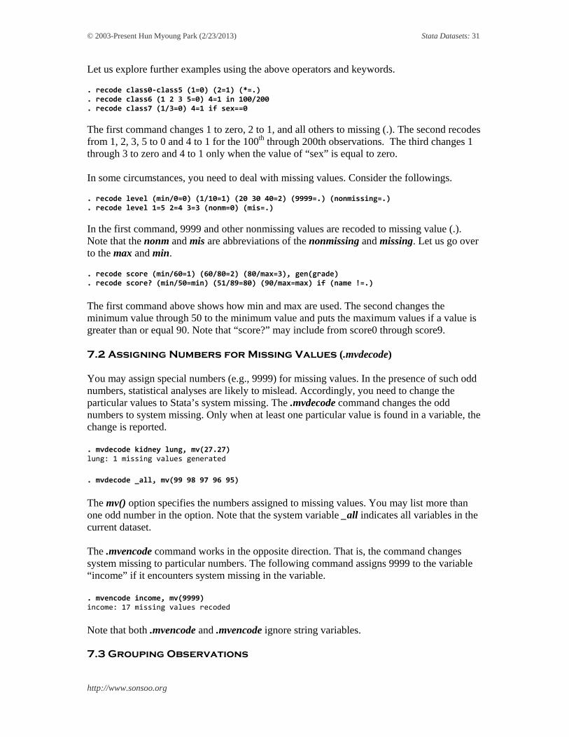
Let us explore further examples using the above operators and keywords. . recode class0‐class5 (1=0) (2=1) (*=.) . recode class6 (1 2 3 5=0) 4=1 in 100/200 . recode class7 (1/3=0) 4=1 if sex==0

The first command changes 1 to zero, 2 to 1, and all others to missing (.). The second recodes from 1, 2, 3, 5 to 0 and 4 to 1 for the 100th through 200th observations. The third changes 1 through 3 to zero and 4 to 1 only when the value of “sex” is equal to zero. In some circumstances, you need to deal with missing values. Consider the followings. . recode level (min/0=0) (1/10=1) (20 30 40=2) (9999=.) (nonmissing=.) . recode level 1=5 2=4 3=3 (nonm=0) (mis=.)

In the first command, 9999 and other nonmissing values are recoded to missing value (.). Note that the nonm and mis are abbreviations of the nonmissing and missing. Let us go over to the max and min. . recode score (min/60=1) (60/80=2) (80/max=3), gen(grade) . recode score? (min/50=min) (51/89=80) (90/max=max) if (name !=.)

The first command above shows how min and max are used. The second changes the minimum value through 50 to the minimum value and puts the maximum values if a value is greater than or equal 90. Note that “score?” may include from score0 through score9. 7.2 Assigning Numbers for Missing Values (.mvdecode) You may assign special numbers (e.g., 9999) for missing values. In the presence of such odd numbers, statistical analyses are likely to mislead. Accordingly, you need to change the particular values to Stata’s system missing. The .mvdecode command changes the odd numbers to system missing. Only when at least one particular value is found in a variable, the change is reported. . mvdecode kidney lung, mv(27.27) lung: 1 missing values generated

. mvdecode _all, mv(99 98 97 96 95)

The mv() option specifies the numbers assigned to missing values. You may list more than one odd number in the option. Note that the system variable _all indicates all variables in the current dataset. The .mvencode command works in the opposite direction. That is, the command changes system missing to particular numbers. The following command assigns 9999 to the variable “income” if it encounters system missing in the variable. . mvencode income, mv(9999) income: 17 missing values recoded

Note that both .mvencode and .mvencode ignore string variables. 7.3 Grouping Observations



Sometimes you need to categorize observations into several groups. Among useful functions are the group(#), autocode(), and recode(). 7.3.1 The group(#) Function You may wish to categorize observations into several groups. The .recode command may work, but the command needs to be repeated several times to do that. The easiest way is to use the group(#) function, which conduct grouping on the basis of order of observations. So a dataset needs to be sorted on the key variable in advance. . sort cigar . gen g1_cigar=group(5)

You need to specify the number of groups in the parenthesis. The above commands classify observations into five groups according to cigarette consumption. The new variable g_cigar has values from 1 through 5. 7.3.2 The autocode() Function The autocode(variable, #, min, max) function partitions the interval of a variable from minimum to maximum into several equal length intervals. The function returns the upper bound of each interval instead of serial numbers (e.g., 1 through 5). Unlike the group(#), you do not need to sort the current dataset. . gen g2_cigar=autocode(cigar, 5, 14, 42.4)

The arguments of the autocode() are a variable name, the number of groups, minimum, and maximum. The interval of each group in this case is 5.68 (=25.36-19.68). You may compare the results of the two functions. . tab g1_cigar g2_cigar

| g2_cigar g1_cigar | 19.68 25.36 31.04 36.72 42.4 | Total ‐‐‐‐‐‐‐‐‐‐‐+‐‐‐‐‐‐‐‐‐‐‐‐‐‐‐‐‐‐‐‐‐‐‐‐‐‐‐‐‐‐‐‐‐‐‐‐‐‐‐‐‐‐‐‐‐‐‐‐‐‐‐‐‐‐‐+‐‐‐‐‐‐‐‐‐‐ 1 | 5 4 0 0 0 | 9 2 | 0 9 0 0 0 | 9 3 | 0 6 2 0 0 | 8 4 | 0 0 9 0 0 | 9 5 | 0 0 5 2 2 | 9 ‐‐‐‐‐‐‐‐‐‐‐+‐‐‐‐‐‐‐‐‐‐‐‐‐‐‐‐‐‐‐‐‐‐‐‐‐‐‐‐‐‐‐‐‐‐‐‐‐‐‐‐‐‐‐‐‐‐‐‐‐‐‐‐‐‐‐+‐‐‐‐‐‐‐‐‐‐

Total | 5 19 16 2 2 | 44

Note that the .tab (or .tabulate) command constructs one-way or two-way tables of frequencies. See Chapter 14 for the details. 7.3.3 The recode() Function Another function for grouping observations is the .recode(variable, n1, n2, n3…). Note that the recode() function differs from the .recode command mentioned in the previous section. . gen g3_cigar=recode(cigar, 10, 20, 30, 40, 50)



If a value of a variable is less than or equal to n1, the function returns n1; n2, if n1 < variable <= n2; n3, if n2 < variable <= n3; and so on.17 . tab g1_cigar g3_cigar

| g3_cigar g1_cigar | 20 30 40 50 | Total ‐‐‐‐‐‐‐‐‐‐‐+‐‐‐‐‐‐‐‐‐‐‐‐‐‐‐‐‐‐‐‐‐‐‐‐‐‐‐‐‐‐‐‐‐‐‐‐‐‐‐‐‐‐‐‐+‐‐‐‐‐‐‐‐‐‐ 1 | 6 3 0 0 | 9 2 | 0 9 0 0 | 9 3 | 0 8 0 0 | 8 4 | 0 9 0 0 | 9 5 | 0 4 3 2 | 9 ‐‐‐‐‐‐‐‐‐‐‐+‐‐‐‐‐‐‐‐‐‐‐‐‐‐‐‐‐‐‐‐‐‐‐‐‐‐‐‐‐‐‐‐‐‐‐‐‐‐‐‐‐‐‐‐+‐‐‐‐‐‐‐‐‐‐ Total | 6 33 3 2 | 44

Compare this cross-table with the previous one to know the difference between the autocode() and recode() functions. Note that 10 is ignored because the minimum value of the variable “cigar” is 14. 7.3.4 Generating a Dummy Variable There are several ways of creating dummy variables. The easiest one is to use .generate and .replace. You must check if a dummy variable is correctly generated in particular when missing values are involved. . gen heavy = cigar > 25

This command assigns 1 to a new variable heavy if the value of cigar is greater than 25 and 0 otherwise. 7.4 Separating Variable You may need to separate a variable into several variables. The following the .separate command creates four variables “area1” though “area4.” . separate area, by(area) storage display value variable name type format label variable label ‐‐‐‐‐‐‐‐‐‐‐‐‐‐‐‐‐‐‐‐‐‐‐‐‐‐‐‐‐‐‐‐‐‐‐‐‐‐‐‐‐‐‐‐‐‐‐‐‐‐‐‐‐‐‐‐‐‐‐‐‐‐‐‐‐‐‐‐‐‐‐‐‐‐‐‐‐‐ area1 byte %12.0g area, area == 1 area2 byte %12.0g area, area == 2 area3 byte %12.0g area, area == 3 area4 byte %12.0g area, area == 4

. list area? +‐‐‐‐‐‐‐‐‐‐‐‐‐‐‐‐‐‐‐‐‐‐‐‐‐‐‐‐‐‐‐‐‐‐‐‐‐‐+ | area area1 area2 area3 area4 | |‐‐‐‐‐‐‐‐‐‐‐‐‐‐‐‐‐‐‐‐‐‐‐‐‐‐‐‐‐‐‐‐‐‐‐‐‐‐| 1. | 3 . . 3 . | 2. | 4 . . . 4 | 3. | 1 1 . . . | 4. | 2 . 2 . . | 5. | 4 . . . 4 |

17 This function is similar to a SAS statement of “g3_cigar= (cigar >10) + (cigar >20) + (cigar >30) + (cigar >40);” In SAS, however, the new variable is coded as 0 through 5 rather than 10 through 50 in this case.



|‐‐‐‐‐‐‐‐‐‐‐‐‐‐‐‐‐‐‐‐‐‐‐‐‐‐‐‐‐‐‐‐‐‐‐‐‐‐|

This .separate command is useful when you create an interaction term of an independent variable and a dummy variable for regression analysis. The following example creates two variables “cig_dum0” and “cig_dum1.” If “cigar” is greater than 20, the variable “cig_dum1” is copied from the “cigar.” Otherwise “cig_dum1” has missing values. By contrast, “cig_dum0” has the values of “cigar” only if the condition does not meet. . separate cigar, by(cigar>20) generate(cig_dum) . replace cig_dum1=0 if cig_dum1==.

7.5 Converting between String and Numeric Variables You may need to convert string variables to numeric variables and vice versa. This section discusses the string() and real() functions as well as the .destring, .decode, and .encode commands. 7.5.1 The string() and real() Functions The string() command converts a numeric variable to a string variable, while the real() function do the opposite way. A string variable in the real() function should have only numbers. . gen num_educ = real(education) . replace point=num_educ*grade if num_educ!=. . gen str_grade = string(grade)

7.5.2 The .destring Command The .destring command has very flexible ways of converting string variables into numeric ones. Suppose you have three string variables “score,” “rate,” and “income” that need to be converted to “score2,” “income2,” and “rate2,” respectively. +‐‐‐‐‐‐‐‐‐‐‐‐‐‐‐‐‐‐‐‐‐‐‐‐‐‐‐‐‐‐‐‐‐‐‐‐‐‐‐‐‐‐‐‐‐‐‐‐‐‐‐‐‐+ | score rate income score2 income2 rate2 | |‐‐‐‐‐‐‐‐‐‐‐‐‐‐‐‐‐‐‐‐‐‐‐‐‐‐‐‐‐‐‐‐‐‐‐‐‐‐‐‐‐‐‐‐‐‐‐‐‐‐‐‐‐| 1. | 557.84 4.5% $45000 557.84 45000 4.5 | 2. | 977.50 10.4% $105000 977.5 105000 10.4 | 3. | 348.87 3.7% $76000 348.87 76000 3.7 | +‐‐‐‐‐‐‐‐‐‐‐‐‐‐‐‐‐‐‐‐‐‐‐‐‐‐‐‐‐‐‐‐‐‐‐‐‐‐‐‐‐‐‐‐‐‐‐‐‐‐‐‐‐+

Let us first convert variable “score” to a numeric variable “score2.” . destring score, generate(score2) float score has all characters numeric; score2 generated as float

The generate() option create a new variable “score2.” You may use the replace option to overwrite the existing variable. The float option explicitly declares the float type instead of the default double. When a variable contains a decimal point, the new variable will be float. Otherwise, the new variable will be integer type.



Now, let us convert string variables that include special characters, such as % and $. The ignore() option lists special characters to be ignored in the variables. Accordingly, the first command below does not work. . destring income rate , generate(income2 rate2) float income contains non‐numeric characters; no generate rate contains non‐numeric characters; no generate

Let us include the ignore() option and run the .destring command again. Note that the number of variables in the generate() option should be equal to the number of variable to be converted. . destring income rate , generate(income2 rate2) ignore("$, %") float income: characters $ removed; income2 generated as float rate: characters % removed; rate2 generated as float

Now, compare the original variables with converted ones. Note that “income2” is a float type variable because 105,000 is out of the range of integer. 7.5.3 The .decode Command You may wish to create a string variable on the basis of the value labels of a numeric variable rather than actual numeric values. The .decode command converts a labeled numeric variable to a string variable using the value labels. . decode area, gen(str_area)

. tab area str_area, nolabel

| str_area area | East Midwest South West | Total ‐‐‐‐‐‐‐‐‐‐‐+‐‐‐‐‐‐‐‐‐‐‐‐‐‐‐‐‐‐‐‐‐‐‐‐‐‐‐‐‐‐‐‐‐‐‐‐‐‐‐‐‐‐‐‐+‐‐‐‐‐‐‐‐‐‐ 1 | 8 0 0 0 | 8 2 | 0 12 0 0 | 12 3 | 0 0 15 0 | 15 4 | 0 0 0 9 | 9 ‐‐‐‐‐‐‐‐‐‐‐+‐‐‐‐‐‐‐‐‐‐‐‐‐‐‐‐‐‐‐‐‐‐‐‐‐‐‐‐‐‐‐‐‐‐‐‐‐‐‐‐‐‐‐‐+‐‐‐‐‐‐‐‐‐‐ Total | 8 12 15 9 | 44

Note that the gen() option specifies the name of new string variable. Thusm, the new variable “str_area” has four string values (i.e., East, Midwest, South, and West) instead of four numeric values from 1 through 4. 7.5.4 The .encode Command Now, you may wish to convert in the opposite direction. The .encode command creates a numeric variable from a string variable. The new variable has unique numbers assigned to corresponding categories of the string variable. In addition, the new variable is labeled with the values of the string variables. . encode str_area, gen(area2) label(area_lab)

Note that the above command generates a new variable “area2,” which is identical to the original variable “area.” The label option specifies the name of the value label; if omitted, the variable name is also used as the value label name.



This .encode command will be useful when you conduct an ANOVA analysis with string right-hand side variables. Unlike SAS, Stata .anova command does not allow string variables as righ-hand side variables. Suppose you wish to compare the mean of annual income by gender and education level. The variable “gender” is coded as “Male” and “Female,” while “education” is as “B.A.” “M.A.” and “Ph.D.” The follow command does not work, giving an error message. . anova income gender education no observations r(2000);

This .encode command enables you to run the ANOVA by converting the string variables. Note that the variable “sex” has 1 for “Male” and 2 for “Female.” Similarly, the numeric values of 1 though 3 of “degree” correspond to the three education levels. . encode gender, gen(sex) label(gender) . encode education, gen(degree) . anova income sex degree

Input Output Conversion string() Numeric variable String variable Numeric value Real() String variable w/o characters Numeric Variable String value .destring String variable Numeric Variable String value .decode Numeric variable w/ label String variable Value label .encode String variable w/ characters Numeric Variable String value (label)

The above table summarizes these functions and commanded mentioned so far. The string() function differs from the .decode command in that the former converts numeric values only, whereas the latter converts the value label of a numeric variable to a string variable. The real() function also differs from the .destring and .encode command in that the former does not allow any character (e.g., %, $, Male) in a string variable. 7.6 Splitting and Concatenating 7.6.1 Splitting Variables: .split You may wish to parse a string variable to several string variables. Like PHP and PERL, Stata supports such functionality through the .split command. Suppose you need to take the email account out of a whole email address. That is, take “kucc625” out from the “[email protected].” . split email, parse(@)

This command parses the string of variable “email” using @, divides the string into two parts, and then store each part to “email1” and “email2.” Thus, “email1” has email account only. If you wish to use more than one character for parsing, each character needs to be double quoted. . split email, parse(";" "." "=char(64)") notrim



Note that the char() function returns an ASCII character corresponding to the ASCII code number. The “=char964)” is equivalent to @. The notrim option does not trim leading and trailing spaces of the original variable before parsing. Suppose you want to take year out of a variable “due_date” containing date. The variable needs to have fixed format, such as mm/dd/yyyy. We may use the .split command to get “due_date3” for year information. . split due_date, parse(/)

7.6.2 Substring Variables: . substr() However, the substr() function provides more efficient way of taking a substring of a string variable. The three arguments of the function are a sting variable, a starting position, and the length of substring, respectively. . gen due_year=substr(due_date, 7, 4)

7.6.3 Useful Sting Functions The above function takes four characters starting at the seventh character from the variable “due_date.” You may combine other string functions, such as the trim(), upper(), lower(), reverse(), length(), and word(). See the Chapter 2.5 for the details. . gen cap_name=substr(upper(trim(last_name)), 1, 3)

The above function first removes leading and tailing blanks of the variable “last_name”; makes the variable uppercased; and then returns the first three characters. 7.6.4 Concatenation When you need to put strings together, use the concatenation operator +. Note that the lower() function returns a lowercased string, and that the ltrim(rtrim()) is equivalent to the trim() function. . gen url="http://"+lower(home) . gen email=ltrim(rtrim(account))+"@"+trim(domain)



8. Handling Datasets This chapter addresses how to manipulate datasets: removing observations and variables, appending, merging, sorting, transposing, reshaping, and collapsing. 8.1 Noting a Dataset (.note) You can add notes to the dataset. This command is followed by a colon (:) and a note. If you want to take a look at all notes added to the dataset, simply run .note. . note: This dataset was manipulated from GSS1972-2012 in 2013 . note

8.2 Comparing Datasets (.cf) This command compares two datasets. You may specify the variables to be compared. _all indicates all variables in the current dataset, while verbose displays detailed information of comparison. . cf _all using cancer, verbose . cf cigar lung using cancer, verbose

8.3 Removing Observations (.keep and .drop) The .keep and .drop commands are used to remove observations or variables. The .keep command removes observations that do not meet the conditions, while the .drop removes observations that meet the conditions. . keep if gender==0 . drop in 5 . keep in ‐2/l . drop if gender==1 in 1/100

Note that “l” in the third command is equivalent to “-1,” representing the last observation. 8.4. Removing Variables (.keep and .drop) The .keep command removes variables that are not listed, while the .drop erases variables listed. Once variables are listed, the if and in qualifiers are not allowed in both commands. . keep gender grade korean math english . drop temp1‐temp5 . drop temp? pro* . drop _all

The last is an example of using the system variable _all. Since the system variable indicates all variables in the current dataset, you need to be very careful when using it. 8.5 Adding Observations to a Dataset (.set obs and .append) The .set obs command changes the number of observation by adding blank observations. The number specified should be greater than the current number of observations. For instance, if a



dataset has 90 observations, the following command append 10 observations with all missing values to make 100 observations in the dataset. . set obs 100

8.6 Combining Datasets 8.6.1 Appending Datasets (.append) The .append (or .app) command appends a Stata data file to a current dataset. If you wish to append other types, such as Excel and ASCII text, first import them into Stata. The two data files need to have the same data structure. Otherwise, mismatched variables will be filled with missing values. . append using c:\stata\data\cancer2 . app using c:\stata\data\cancer2, keep (state cigar l* area)

Note that the keep option limits the variables to be appended. You may not use “-“ operator to specify the range of variables in the option; however, you can still use wildcards of * and ?. Under some circumstances, you may need to duplicate current observations. The following .expand command duplicates all observations twice and append them to the current dataset. . list

+‐‐‐‐‐‐‐‐‐‐‐‐‐‐‐‐‐‐‐‐‐‐‐‐‐‐‐‐‐‐‐‐‐‐‐‐‐‐‐‐‐‐‐‐‐‐‐‐‐‐‐‐‐‐‐‐‐‐‐+ | state cigar bladder lung kidney leukemi area | |‐‐‐‐‐‐‐‐‐‐‐‐‐‐‐‐‐‐‐‐‐‐‐‐‐‐‐‐‐‐‐‐‐‐‐‐‐‐‐‐‐‐‐‐‐‐‐‐‐‐‐‐‐‐‐‐‐‐‐| 1. | AK 30.34 3.46 25.88 4.32 4.9 3 | 2. | AL 18.2 2.9 17.05 1.59 6.15 3 | +‐‐‐‐‐‐‐‐‐‐‐‐‐‐‐‐‐‐‐‐‐‐‐‐‐‐‐‐‐‐‐‐‐‐‐‐‐‐‐‐‐‐‐‐‐‐‐‐‐‐‐‐‐‐‐‐‐‐‐+

. expand 3 (4 observations created) . list

+‐‐‐‐‐‐‐‐‐‐‐‐‐‐‐‐‐‐‐‐‐‐‐‐‐‐‐‐‐‐‐‐‐‐‐‐‐‐‐‐‐‐‐‐‐‐‐‐‐‐‐‐‐‐‐‐‐‐‐+ | state cigar bladder lung kidney leukemi area | |‐‐‐‐‐‐‐‐‐‐‐‐‐‐‐‐‐‐‐‐‐‐‐‐‐‐‐‐‐‐‐‐‐‐‐‐‐‐‐‐‐‐‐‐‐‐‐‐‐‐‐‐‐‐‐‐‐‐‐| 1. | AK 30.34 3.46 25.88 4.32 4.9 3 | 2. | AL 18.2 2.9 17.05 1.59 6.15 3 | 3. | AK 30.34 3.46 25.88 4.32 4.9 3 | 4. | AK 30.34 3.46 25.88 4.32 4.9 3 | 5. | AL 18.2 2.9 17.05 1.59 6.15 3 | 6. | AL 18.2 2.9 17.05 1.59 6.15 3 | +‐‐‐‐‐‐‐‐‐‐‐‐‐‐‐‐‐‐‐‐‐‐‐‐‐‐‐‐‐‐‐‐‐‐‐‐‐‐‐‐‐‐‐‐‐‐‐‐‐‐‐‐‐‐‐‐‐‐‐+

You may specify a subset to be duplicated using the if and in qualifiers. . expand 2 if state=="IN" | state=="IL" . expand 5 in ‐10/‐1

8.6.2 Adding Variables or Updating a Dataset (.merge)



The .merge (or .mer) command adds variables to the current dataset from the using dataset. The unmatched variables of the using dataset are added to the master dataset (the current dataset), while the matched replaces corresponding variables in the master dataset. This section ignores the one-to-one merge to focus on the match merge.18 You need a key variable that exist in both datasets. The key variable must have the same name and the same data type, and should be sorted in advance. In the following example, “state” is the key variable by which observations are matched. . sort state . merge 1:1 state using cancer2

The command creates and adds a new variable called “_merge” that indicates the data sources of observations. When data of an observation are from the master dataset, the _merge is set 1. The 2 indicates that the observation came from the using dataset. For observations from the both dataset, 3 is assigned to the _merge.

The .merger command by default does not change information in the master dataset even when the using dataset has updated information. If you wish to update information, add the update and replace options. The replace option cannot be used individually, but should be use with the update option. . sort state . merge 1:1 state using cancer2, update replace

Under the update option, missing values of the master dataset are replaced with nonmissing values of the using dataset. The update replace options replace nonmissing values of the master dataset with new information in the using dataset. But in any case, nonmissing values are not replaced with missing values of the using dataset. Values of the Master Unspecified Update Update & Replace Nonmissing Unchanged Unchanged Replaced Missing Unchanged Replaced Replaced

When the update option is specified, the code 3 of the _merge (i.e., observation from both datasets) is broken into three categories. New code 3 indicates that both datasets have the same information; 4 is set when missing values of the master are replaced with nonmissing values. If nonmissing values of the master are replaced, the _merge has 5. You may use a different name instead of the default “_merge.” The following command creates a variable “code.” . merge 1:1 state using cancer2, update replace _merge(code)

This command supports one to many merge (1:m) and many to one merge (m:1), and many to many merge (m:m). Suppose you are matching a homework records (multiple observations

18 The one-to-one merge just mechanically put two datasets together. The first observation of the master dataset is joined to the first one of the using dataset. The second is joined to the second of the using dataset. So this type of merge does not need any key variable. In the match merge, by contrast, an observation is joined to corresponding one only if their key variable is matched. In a practical sense, one-to-one merge is less useful than the match merge.



per a student) with student registration file (unique). You can merge two files using .merge m:1 as follows. . merge m:1 id using student, unmatched(both)

In old releases (before 11), .joinby conducts many to one merge as follows. . joinby id using student, unmatched(both)

8.7. Sorting Observations and Variables 8.7.1 Sorting (.sort) Some commands and functions require that a dataset is sorted in some ways. The .sort (or .so) command arranges observations in ascending order with respect to variables listed. You may use the in qualifier to limit the range of observations. . sort grade . sort grade name in 10/100

Note that “grade” and “name” in the second command are respectively used as primary and secondary keys. 8.7.2 Descending Sorting (.gsort) This command arranges data in ascending or descending order. In case of the descending order, you need to add hyphen (–) before the variable name. . gsort +cigar . gsort -cigar 8.7.3 Sorting Variables (.order and .move) Why are we bothered with the order of variables? We can benefit from well arranging variables of a huge dataset. The most prominent advantage exists in the use of wildcard – (e.g., cigar-kidney). The .stack command does not use the variable order listed in the command, but the physical order of variables in a dataset. The .order and .move commands are used to rearrange the order of variables. The former rearrange variables as listed, while the latter moves the location of the first variable to the next of the second variable, holding other variables unchanged. . order firstName lastName grade . move avg total

Note that the .move command can have only two variable names. 8.8. Compressing Datasets (.compress) This command compresses the dataset to make its file size smaller. The types of some variables may be changed in compression. 8.9. Removing Datasets from Memory (.clear)



The .clear command removes current dataset, label, matrices, scalars, cluster, and constraints from the memory. . clear . drop _all

Unlike the .clear, the .drop _all just removes the current dataset by erasing all variables and observations, leaving labels, matrices and others unchanged. 8.10. Deleting Datasets (.erase and .rm) If you wish to delete datasets from the disk, use the .erase or the .rm command. Note that the .rm, a UNIX command to erase files, does not work in Stata for Windows. . erase c:\stata\data\cancer_temp.dta



9. Reshaping Datasets This chapter addresses various ways of reshaping a dataset. This feature is important especially when handling panel data and dataset for ANOVA. 9.1 Getting Aggregate Statistics Often times it is necessary to compute aggregate statistics such as sum and mean of groups. 9.1.1 Getting a Dataset of Summary Statistics (.collapse) You may wish to save aggregate statistics, such as mean and standard deviation, to a dataset. Like SAS MEANS procedure, the .collapse command can do the job using the keywords of statistics. The command replaces the current dataset with a new one containing aggregate statistics. Frequently used keywords include mean, sum, sd (standard deviation), count (the number of observation), max, min, and median (or p50). The default mean can be omitted. . collapse cigar (sum) bladder (sd) lung (count) kidney (max) leukemia

The above command creates a dataset that has one observation with five variables. Variable names are copied to the new dataset. Note that you cannot specify more than one keyword at a time. . collapse (mean) cigar (sum) cig_sum=cigar (sd) cig_sd=cigar lung

This command demonstrates how to get various statistics of a variable. Note that you need to provide target variable names using the = operator; variable names should be unique in a dataset. For example, standard deviation of the variable “cigar” is stored in a variable “cig_sd.”

You may wish to get aggregate statistics arranged by group. Like the BY statement in SAS, the by option computes statistics group by group. . collapse cigar (max) bladder (p50) lung (p75) kidney, by(area) . list +‐‐‐‐‐‐‐‐‐‐‐‐‐‐‐‐‐‐‐‐‐‐‐‐‐‐‐‐‐‐‐‐‐‐‐‐‐‐‐‐‐‐‐‐‐‐‐‐‐‐‐‐+ | area cigar bladder lung kidney | |‐‐‐‐‐‐‐‐‐‐‐‐‐‐‐‐‐‐‐‐‐‐‐‐‐‐‐‐‐‐‐‐‐‐‐‐‐‐‐‐‐‐‐‐‐‐‐‐‐‐‐‐| 1. | East 27.94625 5.98 22.435 3.195 | 2. | Middlewest 23.706667 5.27 18.57 3.04 | 3. | South 24.208667 5.6 19.45 3.13 | 4. | West 25.004444 6.54 19.5 2.78 | +‐‐‐‐‐‐‐‐‐‐‐‐‐‐‐‐‐‐‐‐‐‐‐‐‐‐‐‐‐‐‐‐‐‐‐‐‐‐‐‐‐‐‐‐‐‐‐‐‐‐‐‐+

Thus, the above command produces four observations corresponding to four different areas. Note that the variable “area” was added as the first variable in a new dataset. 9.1.2 Getting a Dataset of Summary Statistics (.contract) Another useful command is the .contract, which creates a dataset of frequencies. Suppose you want to count the frequencies of all possible combinations of “gender,” “degree,” and “area”. This command is more flexible than the .tabulate.



.contract gender degree area, freq(count) zero nomiss

. list +‐‐‐‐‐‐‐‐‐‐‐‐‐‐‐‐‐‐‐‐‐‐‐‐‐‐‐‐‐‐‐‐‐‐‐‐‐‐‐‐‐+ | gender degree area count | |‐‐‐‐‐‐‐‐‐‐‐‐‐‐‐‐‐‐‐‐‐‐‐‐‐‐‐‐‐‐‐‐‐‐‐‐‐‐‐‐‐| 1. | Female B.A. Citizen 3 | 2. | Female B.A. International 9 | 3. | Female M.A. Citizen 0 | 4. | Female M.A. International 5 | 5. | Male B.A. Citizen 8 | |‐‐‐‐‐‐‐‐‐‐‐‐‐‐‐‐‐‐‐‐‐‐‐‐‐‐‐‐‐‐‐‐‐‐‐‐‐‐‐‐‐| 6. | Male B.A. International 4 | 7. | Male M.A. Citizen 0 | 8. | Male M.A. International 7 | +‐‐‐‐‐‐‐‐‐‐‐‐‐‐‐‐‐‐‐‐‐‐‐‐‐‐‐‐‐‐‐‐‐‐‐‐‐‐‐‐‐+

Note that the freq option specifies variable name that store the frequency of each case; the default variable name is “_freq.” The zero option includes cases even when their frequencies are zero, while the nomiss excludes cases in which at least one of variables is missing. 9.2 Stacking Up a Dataset Stata can put variables together by vertically stacking up them. The feature is handy in handling multiple choice questions. 9.2.1 Reshaping (.reshape) Suppose you have multiple choice questions that asked subjects to pick three out of 10 choices. This is called the wide format in Stata. . list +‐‐‐‐‐‐‐‐‐‐‐‐‐‐‐‐‐‐‐‐‐‐‐‐‐‐‐‐‐‐‐‐‐‐‐‐‐‐‐+ | subject choice1 choice2 choice3 | |‐‐‐‐‐‐‐‐‐‐‐‐‐‐‐‐‐‐‐‐‐‐‐‐‐‐‐‐‐‐‐‐‐‐‐‐‐‐‐| 1. | 1 5 8 9 | 2. | 2 1 2 8 | 3. | 3 1 2 3 | 4. | 4 2 5 8 | 5. | 5 2 5 8 | +‐‐‐‐‐‐‐‐‐‐‐‐‐‐‐‐‐‐‐‐‐‐‐‐‐‐‐‐‐‐‐‐‐‐‐‐‐‐‐+

In order to analyze such questions, you need to stack up the three choices into one variable: the long format in Stata. The .reshape and .stack commands are the case. Let us first consider an example of the .reshape command. . reshape long choice, i(subject) j(orders) (note: j = 1 2 3) Data wide ‐> long ‐‐‐‐‐‐‐‐‐‐‐‐‐‐‐‐‐‐‐‐‐‐‐‐‐‐‐‐‐‐‐‐‐‐‐‐‐‐‐‐‐‐‐‐‐‐‐‐‐‐‐‐‐‐‐‐‐‐‐‐‐‐‐‐‐‐‐‐‐‐‐Number of obs. 5 ‐> 15 Number of variables 4 ‐> 3 j variable (3 values) ‐> orders xij variables: choice1 choice2 choice3 ‐> choice ‐‐‐‐‐‐‐‐‐‐‐‐‐‐‐‐‐‐‐‐‐‐‐‐‐‐‐‐‐‐‐‐‐‐‐‐‐‐‐‐‐‐‐‐‐‐‐‐‐‐‐‐‐‐‐‐‐‐‐‐‐‐‐‐‐‐‐‐‐‐‐



The long option converts to the long format. The i and j respectively indicate the unique variable and the number of variables to be stacked. You may specify particular values in the j option like “j(weight 10 20 30)” or “j(year 2000-2003).” . list +‐‐‐‐‐‐‐‐‐‐‐‐‐‐‐‐‐‐‐‐‐‐‐‐‐‐+ | subject orders choice| |‐‐‐‐‐‐‐‐‐‐‐‐‐‐‐‐‐‐‐‐‐‐‐‐‐‐| 1. | 1 1 5 | 2. | 1 2 8 | 3. | 1 3 9 | 4. | 2 1 1 | 5. | 2 2 2 | |‐‐‐‐‐‐‐‐‐‐‐‐‐‐‐‐‐‐‐‐‐‐‐‐‐‐| 6. | 2 3 8 | 7. | 3 1 1 | 8. | 3 2 2 | 9. | 3 3 3 | 10. | 4 1 2 | |‐‐‐‐‐‐‐‐‐‐‐‐‐‐‐‐‐‐‐‐‐‐‐‐‐‐| 11. | 4 2 5 | 12. | 4 3 8 | 13. | 5 1 2 | 14. | 5 2 5 | 15. | 5 3 8 | +‐‐‐‐‐‐‐‐‐‐‐‐‐‐‐‐‐‐‐‐‐‐‐‐‐‐+

Now you are ready to analyze the frequency of the variable “choice.” If you wish to convert back to the wide format, run the following command. . reshape wide

9.2.2 Stacking Up (.stack)

Another useful command is .stack, which stacks variables up vertically. In the following example, variables “best1” through “best3” are vertically stacked into variable “best,” while “worst1” through “worst3” are stacked into “worst.” . list +‐‐‐‐‐‐‐‐‐‐‐‐‐‐‐‐‐‐‐‐‐‐‐‐‐‐‐‐‐‐‐‐‐‐‐‐‐‐‐‐‐‐‐‐‐‐‐‐‐‐+ | best1 best2 best3 worst1 worst2 worst3 | |‐‐‐‐‐‐‐‐‐‐‐‐‐‐‐‐‐‐‐‐‐‐‐‐‐‐‐‐‐‐‐‐‐‐‐‐‐‐‐‐‐‐‐‐‐‐‐‐‐‐| 1. | 1 2 3 4 5 6 | 2. | 7 8 9 10 11 12 | +‐‐‐‐‐‐‐‐‐‐‐‐‐‐‐‐‐‐‐‐‐‐‐‐‐‐‐‐‐‐‐‐‐‐‐‐‐‐‐‐‐‐‐‐‐‐‐‐‐‐+ . stack best1‐best3 worst1‐worst3, into(best worst) clear . list +‐‐‐‐‐‐‐‐‐‐‐‐‐‐‐‐‐‐‐‐‐‐‐+ | _stack best worst | |‐‐‐‐‐‐‐‐‐‐‐‐‐‐‐‐‐‐‐‐‐‐‐| 1. | 1 1 2 | 2. | 1 7 8 | 3. | 2 3 4 | 4. | 2 9 10 | 5. | 3 5 6 | 6. | 3 11 12 | +‐‐‐‐‐‐‐‐‐‐‐‐‐‐‐‐‐‐‐‐‐‐‐+



Note that the number of variables to be stacked should be equal over output variables. In the above example, the into option cannot have four or five variables. Similarly, the following also does not work. . stack a b c d e f g h, into(stack1‐stack3) clear

You may alternatively use the group(#) option instead of the into as follow. Note that the first two variable names (“best1” and “best2”) will be used in the new dataset. . stack best1‐best3 worst1‐worst3, group(2) clear

The .stack command uses the physical order of variables no matter how variables are listed in the command. Accordingly, the following does not make any difference. See the section 6 for details about how to change the physical order of variables. . stack best1 worst1 best2 worst3 best3 worst3, group(2) clear

9.2.3 Reshaping for Latin Square Design (.pkshape)

If you have a tabulated data for Latin Square design, use the .pkshape command that reshapes the data set for ANOVA. Suppose your experiment data look like,

1st Test 2nd Test 3rd Test Subject 1 74 (a) 57 (b) 50 (c) Subject 2 6 (c) 94 (a) 78 (b) Subject 3 40 (b) 29 (c) 112 (a)

Source: Dowdy, Wearden, and Chilko (2004), p365.

You may enter the data in Stata as follows. . list id row col1‐col3, noobs +--------------------------------+ | id row col1 col2 col3 | |--------------------------------| | 100 1 74 57 50 | | 101 2 6 94 78 | | 102 3 40 29 112 | +--------------------------------+

Now, run the .pkshape command to reshape the data set. The order() option specifies treatments beginning from the top and left. Note that the outcome(), sequence(), treat(), and period() options have their default values as their names. . pkshape id row col1-col3, order(abc cab bca) /// outcome(y) sequence(rows) treat(treat) period(columns)

The result looks like, +--------------------------------------------+ | id rows y treat carry columns | |--------------------------------------------| | 100 1 74 1 0 1 | | 101 2 6 3 0 1 | | 102 3 40 2 0 1 | | 100 1 57 2 1 2 | | 101 2 94 1 3 2 | | 102 3 29 3 2 2 | | 100 1 50 3 2 3 | | 101 2 78 2 1 3 |



| 102 3 112 1 3 3 | +--------------------------------------------+

You are ready to conduct ANOVA as follows. . anova y rows columns treat Number of obs = 9 R-squared = 0.9984 Root MSE = 2.64575 Adj R-squared = 0.9936 Source | Partial SS df MS F Prob > F -----------+---------------------------------------------------- Model | 8752 6 1458.66667 208.38 0.0048 | rows | 2 2 1 0.14 0.8750 columns | 2400 2 1200 171.43 0.0058 treat | 6350 2 3175 453.57 0.0022 | Residual | 14 2 7 -----------+---------------------------------------------------- Total | 8766 8 1095.75

9.3 Rectangularizing Dataset (.fillin) 9.4 Transposing a Dataset (.xpose) Sometimes you need to transpose a dataset. The .xpose, clear command switches observations and variables. In other words, the command changes rows into columns and columns into rows. The clear option is required in this command, since the current dataset is removed out of the memory. . xpose, clear varname . list +‐‐‐‐‐‐‐‐‐‐‐‐‐‐‐‐‐‐‐‐‐‐‐‐‐‐‐‐‐‐‐‐‐‐‐‐‐‐‐‐‐‐‐‐‐‐‐‐‐‐‐‐‐‐+ | v1 v2 v3 v4 _varname | |‐‐‐‐‐‐‐‐‐‐‐‐‐‐‐‐‐‐‐‐‐‐‐‐‐‐‐‐‐‐‐‐‐‐‐‐‐‐‐‐‐‐‐‐‐‐‐‐‐‐‐‐‐‐| 1. | 1 2 3 4 area | 2. | 27.94625 23.70667 24.20867 25.00444 cigar | 3. | 5.98 5.27 5.6 6.54 bladder | 4. | 22.435 18.57 19.45 19.5 lung | 5. | 3.195 3.04 3.13 2.78 kidney | +‐‐‐‐‐‐‐‐‐‐‐‐‐‐‐‐‐‐‐‐‐‐‐‐‐‐‐‐‐‐‐‐‐‐‐‐‐‐‐‐‐‐‐‐‐‐‐‐‐‐‐‐‐‐+

The varname option adds a variable that contains variable names of the original dataset. The option is recommended because it makes the dataset more readable. Note that the labels of the original dataset are ignored; actual numeric values are copied to the new dataset instead.



10. Advanced Topics This chapter addresses advanced topics in which intermediate or sophisticated Stata users may have interests. 10.1 Missing Values 10.1.1 Summarizing Missing Values (.misstable) This command provides missing value information in the table form. The first command below summarizes missing value information in the current dataset, while the second suggest missing value patters. . misstable summarize . misstable patterns

10.1.2 Marking Missing Values (.mark and .markout) The missing value of a numeric variable is conventionally denoted by a single period (.). In string, missing value is expressed as “”. Any arithmetic operation on a missing value results in a missing value. Users may wish to exclude missing values using the if qualifier. You may ask whether a variable is less than period (.). . sum cigar lung kidney if cigar<. . list cigar lung kidney if (cigar==.) | (lung>.) | (kidney>=.)

The first command above produces summary statistics of those observations whose variable “cigar” is not missing. The second lists the values of three variables when any one of the three is missing. Note that the three different usages of relational operators equally detect missing values in each variable. You may want to detect observations that have missing values in any variables specified. The .mark and .markout commands are useful for marking observations with the missing. The former command creates a dummy variable to be used by the latter. The .markout command sets 0 in the marking variable created by the .markout command if an observation has missing values. . mark yn_miss // to create a marking variable (dummy) . mark yn_miss cigar lung kidney . tab yn_miss, missing // to double-check flagging marks . drop if yn_miss==0 // to drop observations with missing values 10.1.3 From Missing to Numeric Values (.mvencode) 10.1.4 From Numeric Values to Missing (.mvdecode) 10.2 Imputation (.impute)



10.3 Duplicates 10.3.1 Checking Unique Identifiers (.isid) You may want to know whether there is any duplicate observation with respect to particular variables. The .isid command checks whether specified variables identify observations uniquely. . isid name variable name does not uniquely identify the observations r(459);

If listed variables cannot identify observation uniquely, Stata will give you a warning message. The result above indicates that there is at least one duplicate name in the variable “name.” You may list more than one variable. . isid gender degree area

10.3.2 Detecting Duplicates (.duplicates) The .duplicates command detects, lists, tags, and drops duplicate observations. This command is very useful especially for data cleaning. The following command with the examples (or e) subcommand shows examples of duplicate observations with respect to “gender,” degree,” and “area.” . duplicates examples gender degree area

+‐‐‐‐‐‐‐‐‐‐‐‐‐‐‐‐‐‐‐‐‐‐‐‐‐‐‐‐‐‐‐‐‐‐‐‐‐‐‐‐‐‐‐‐‐‐‐‐‐‐‐‐‐‐‐‐‐+ | group: # e.g. obs gender degree area | |‐‐‐‐‐‐‐‐‐‐‐‐‐‐‐‐‐‐‐‐‐‐‐‐‐‐‐‐‐‐‐‐‐‐‐‐‐‐‐‐‐‐‐‐‐‐‐‐‐‐‐‐‐‐‐‐‐| | 1 3 6 Female B.A. Citizen | | 2 9 5 Male M.A. International | +‐‐‐‐‐‐‐‐‐‐‐‐‐‐‐‐‐‐‐‐‐‐‐‐‐‐‐‐‐‐‐‐‐‐‐‐‐‐‐‐‐‐‐‐‐‐‐‐‐‐‐‐‐‐‐‐‐+

Stata identified two duplicate patterns. Three are three observations (including the sixth observation) for the first pattern and nine observations for the second. Note its format is similar to that of the .contract command in the previous section. You may want to list the duplicate observations detected. Use the .list (or l) or .browse (or b) subcommand. . duplicates list gender degree area

You may also tag duplicate observations by creating a variable storing the frequency of each case. The tag (or t) subcommand assigns 1 to the tag variable “dup_tag” if an observation is unique. . duplicates tag gender degree area, generate(dup_tag)

Note that the generate() option for specifying a variable name is required in the tag subcommand.



Finally, you may wish to drop duplicate observations to make the dataset unique in terms of the variables listed. Use the drop subcommand to remove all duplicate observations except the first one of the duplicate pattern. . duplicates drop gender degree area, force

Note that the force option is required when variables are listed in the drop subcommand. 10.3.3 Duplicating Observation (.expand) See append 10.3.4 Duplicating Clustered Observations (.expandcl) 10.4 Weighting 10.5 Resampling 10.6.1 Sampling (.sample) 10.6.2 Drawing from Normal Distribution (.drawnnorm) 10.6 Random Number Generation

Documents

2. Creating and Saving Datasets - 国際大学 · . u c:\stata\data\cancer if area==1, clear nol The first command loads first 10 observations from the dataset, while the second reads