1

Departament de Genètica Facultat de Biologia

Universitat de Barcelona

MODELS DE XARXES GÈNIQUES EN EL DESENVOLUPAMENT

EMBRIONARI I L’EVOLUCIÓ

GENE NETWORK MODELS IN EMBRYONARY DEVELOPMENT AND EVOLUTION

ISAAC SALAZAR CIUDAD

Barcelona 2001

2

Memòria presentada per Isaac Salazar Ciudad per aspirar al grau de Doctor en Ciències Biologiques. Tesi realitzada sota la direcció dels Drs. Ricard Vicente Solé i Jordi Garcia-Fernàndez al Departament de Genètica de la Facultat de Biologia de la Universitat de Barcelona i al Departament de Física i Enginyeria Nuclear de la Universitat Politècnica de Catalunya. Programa de Genètica (Bienni 1997-1999) Barcelona, Novembre 2001 Vist i plau de: DIRECTOR AUTOR DIRECTOR

Dr. Jordi Garcia-Fernàndez Isaac Salazar Ciudad Ricard Vicente Solé Professor Titular Professor Titular Dept. de Genètica Dept. Física i Eginyeria Facultat de Biologia Nuclear Universitat de Barcelona Universitat Politècnica de Catalunya

3

4

"Nothing in Biology makes sense except in the light of evolution" T. Dobzhansky (1900-1975)

5

6

Used abreviations: DM: Developmental mechanism MDM: Morphodynamic developmental mechanism

MSM: Morphostatic developmental mechanism

7

8

Index: Foreword 13 Resum en català 15 Introduction 1.1 Introduction 23 1.2 Basic principle of evolution 1.2.1 Basic principle of evolution 24 1.2.2 Temporal scale 24 1.2.3 Causality and grain of the selective pressures imposed by the environment 27 1.2.4 Towards a generative and dynamical theory of evolution or a minimal complete theory of evolution 29 1.3 Used concepts 1.3.1 Complexity and information 35 1.3.2 Causal forces in evolution 36 1.3.3 The environment: the phenotype selection interdependence 36 1.3.4 Internal structure: levels of organization 41 1.3.5 Developmental mechanism 42 1.4 E-C paradox 46 1.5 Objectives 49 Methods 2.1 Theories of the origin of information 2.1.1 Theories of the origin of information: Evolutionarily interesting properties of a DM 51 2.1.2 Theories of the genesis of the information: potential predictions 53 2.1.3 Theories of the genesis of information: types of mechanisms in metazoan 2.1.3.1 Molecular level 54 2.1.3.2 Cellular level 55 2.2 A classical description of development 56 2.3 An actualised description of development 61 Results: 3. Systems with only cell communication: Gene networks capable of pattern formation: 3.1 Introduction 65 3.2 The paper: Salazar-Ciudad, Garcia-Fernàndez, J and Solé, R.V.,Gene networks capable of pattern formation: from induction to reaction-diffusion. Published in journal of

theoretical biology. 654. Variational properties of systems using only cell communication

9

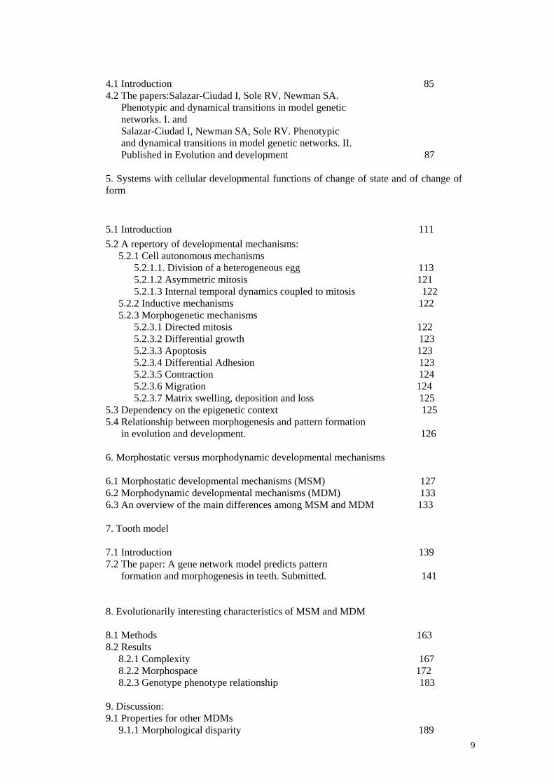
4.1 Introduction 85 4.2 The papers:Salazar-Ciudad I, Sole RV, Newman SA. Phenotypic and dynamical transitions in model genetic networks. I. and Salazar-Ciudad I, Newman SA, Sole RV. Phenotypic and dynamical transitions in model genetic networks. II. Published in Evolution and development 87 5. Systems with cellular developmental functions of change of state and of change of form

5.1 Introduction 111 5.2 A repertory of developmental mechanisms: 5.2.1 Cell autonomous mechanisms 5.2.1.1. Division of a heterogeneous egg 113 5.2.1.2 Asymmetric mitosis 121 5.2.1.3 Internal temporal dynamics coupled to mitosis 122 5.2.2 Inductive mechanisms 122 5.2.3 Morphogenetic mechanisms 5.2.3.1 Directed mitosis 122 5.2.3.2 Differential growth 123 5.2.3.3 Apoptosis 123 5.2.3.4 Differential Adhesion 123 5.2.3.5 Contraction 124 5.2.3.6 Migration 124 5.2.3.7 Matrix swelling, deposition and loss 125 5.3 Dependency on the epigenetic context 125 5.4 Relationship between morphogenesis and pattern formation in evolution and development. 126 6. Morphostatic versus morphodynamic developmental mechanisms 6.1 Morphostatic developmental mechanisms (MSM) 127 6.2 Morphodynamic developmental mechanisms (MDM) 133 6.3 An overview of the main differences among MSM and MDM 133 7. Tooth model 7.1 Introduction 139 7.2 The paper: A gene network model predicts pattern formation and morphogenesis in teeth. Submitted. 141 8. Evolutionarily interesting characteristics of MSM and MDM 8.1 Methods 163 8.2 Results 8.2.1 Complexity 167 8.2.2 Morphospace 172 8.2.3 Genotype phenotype relationship 183 9. Discussion: 9.1 Properties for other MDMs 9.1.1 Morphological disparity 189

10

9.1.2 Complexity 193 9.1.3 Relationship between phenotype and genotype 193 9.1.4 Form of the morphospace 195 9.1.5 Homeostasis 205 9.2 Predictions 9.2.1 Dynamics of apparition and substitution among DMs 205 9.2.2 The structure of development 208 9.2.3 Phylogeny, disparity and environment 210 9.3 Existing evidence 9.3.1 Experimental evidence for MDM 212 9.3.2 Research problems with MDM 216 9.3.3 Examples of substitution among DMs 218 9.3.4 Disparity and time since last common ancestor 219 9.3.5 Variational properties of development and general characteristics of development 220 9.4 Generalities: 9.4.1 Evolutionary dynamics from the theories of the origin of information 223 9.4.2 Conceptual changes in the way to look at evolution induced by the theories of the origin of information: 9.4.2.1 Evolutionary dynamics 224 9.4.2.2 New approaches for old questions 226 9.4.2.3 Questions about why 228 9.4.3 Merging emergent networks, form DMs and MDMs 229 9.4.4 Generalizations to other systems 230 10. Conclusions 233 11. Acknowlodgements 237 12. Bibliography 239 Annex I: Program used for the simulations in section 3.2 251 Annex II:Program used for the simulations in section 4.2: selection simulations 259 Annex III:Program used for the simulations in section 4.2: simulation of networks 289 Annex IV:Program used for the simulations in section 7.2 309 Annex V: Solé RV, Salazar-Ciudad, I, Newman, SA. Gene network dynamics and the evolution of development 2000 published in Trends in ecology and evolution. 323 Annex VI: Solé RV, Salazar-Ciudad, I, Garcia-Fernàndez J. Landscapes, Gene Betworks and Pattern Formation: on the Cambrian

Explosion. 1999 published in Advances in complex systems 327

11

0. Foreword:

This thesis includes the most relevant work I have done since I finish my career in Biology. It is not a definitive version of nothing as a product of scientific research never is. In fact it deals with ever-changing ideas about how nature works, that as science, are likely to be flawed. Some effort is made to present it as a closed work, at least in some sense. And I think that to some extent it is. In essence, this thesis includes a considerable chunk of ideas that can be valuable in isolation but that constitute a inter-supporting framework useful for thinking in the emergence of a more complete theory of evolution (or at least a different way to approach it). The thesis is thus written in order to facilitate to the reader the understanding of the intrinsically complex dynamics of evolution (and of the way to approach it). The question approached is not easy an many new concepts are used that, as newly developed concepts, may not be presented in the more understandable way (although I tried). Of course the reader can always think that most persons talking about their own work will always say that it is complex, and that many things will not seem so complex if stated in another way. The best way to read this thesis is to read it straight through. The thesis is written for readers that have a considerable previous knowledge of the topics studied. Unfortunately, it is not very usual that scientist have a very similar framework (everybody is always more interested in some topics) but in the case of the topics with which I deal this is specially true because these topics have been traditionally studied in a compartmentalized way. This compartmentalization does not coincide with the one I use. I hope that the logic for such iconoclasy will become apparent after having a close look to the reasoning and results here written. Some of the results are published and submitted articles but the main body of the thesis is not in an article aesthetics. There are many things that are more easily presented by non using a scientific article format. This thesis is one of these. It is presented as a presentation of a theory, or more correctly of a theoretical framework. It includes then an introduction that presents why this theory is needed (that implies to say what may be wrong with the other related theories). Later, but still in the introduction, I introduce some concepts that are not true or false, just nomenclature. In the methods I superficially describe which kind of thing the theory I present will be able to ask and answer and, in a general way, how it will be answered. In the results I actually present and apply the theory and its methodology in general and concrete cases. In the discussion I describe which implications has the theory, to which extent it explains what it is supposed to explain, how it fits some other data not considered in the concrete applications presented in the results, how it can be improved and

12

generalized (if it can actually be done) and which potential flaws it can have (and how to solve them).

My interest for the study of development and evolution is not casual. It comes from the perception that there is a huge gap between what current evolutionary theory is able to satisfactorily explain and what we observe in nature (even if some of the basic tools to understand it, the basic principle of evolution for example, are already at hand). One of the more important things of life is the observable disparity of phenotypes. It is a problem that is not addressed correctly by current evolutionary theory since this theory can not predict much about the structure of organisms (except for the molecular level in some cases). Later, once embedded in the inclusion of the generative properties of live in the evolutionary theory, I realized that a successful inclusion requires a new perspective that transforms the theory so dramatically that it can not longer be said that development is simply included (although the basics of neo-Darwinian theory can be said to be still there). At the same time we expect that the principles of this incipient theory may be applicable to a wide class of complex systems and not necessarily only to the life we know. So it is not that I chosen the issue of my research because I had an special facility with it but because I wanted to understand the maximum number of things with the minimum effort and I perceive that complex systems are a big proportion of existing systems (although they may occupy relatively few space in the universe). Among them we though that the ones that I will call evolutive systems (mainly living beings) are the ones that can attain more complexity and more often. In addition, or at least, they are the more well know and more easy to study, so, I though that it is a quick strategy to try to understand this more accessible systems that can be at the same time useful for understanding many others. In fact the choosing of an exclusively theoretical methodology has been posterior to the choosing of my objective of research. Being aware of the likely fintiness of my life duration and interested in things able to explain as many things as possible in a simple and true-prone way I was biased to approaches with an important theoretical component. That it has been exclusively theoretical is due to the difficulty to coordinate a theoretical approach and a experimental one. On the other hand more than two decades of self-knowledge dissuaded me to enter in a technified world in which order, tidiness and patience are praiseable virtues.

13

Resum de la tesis en català:

Abstract of the thesis in catalan: Introducció: La teoria evolutiva té com a objectiu explicar la diversitat i disparitat dels organismes vius. Aquesta estableix que les poblacions tenen variabilitat fenotípica heredable que en el medi afecta la contribució relativa dels diferents individus d’una població en la següent generació. A més, la teoria estableix que aquest procés s afectat per dependències històriques i fenòmens atzarosos com ara la deriva gènica. La causa última de la variació fenotípica rau en mutacions que són essencialment atzaroses (malgrat més probables en certes regions del DNA). Això, però, no explica quin tipus de variacions morfològiques són possibles en un llinatge concret. De fet, la teoria Darwinista ens ajuda a entendre com diferents variants en les poblacions es substitueixen unes a altres però no com o perquè apareixen unes variacions o unes altres (excepte a nivell molecular). L’objectiu d’aquesta tesi és introduir certs aspectes de com el desenvolupament funciona per tal de que la teoria evolutiva, o una variant d’aquesta, tingui un cert poder predictiu sobre l’estructura del fenotip. A part, això, pot ajudar a entendre quins factors, i com, afecten la evolució dels metazous. El desenvolupament és també un producte de l’evolució. Fent el que acabem d’esmentar també aconseguim desenvolupar un marc teòric que ens permeti estudiar evolució i desenvolupament unificadament.

Mètodes: La nostra intenció ha estat veure què és capaç de fer teòricament el desenvolupament. En base a com és el desenvolupament això és difícil d’establir ja que el desenvolupament present és un producte de la història i la selecció de forma que no reflexa únicament allò que és possible (que és el que ens interessa, perquè per establir com ha anat l’evolució ens cal saber que és possible i perquè només trobem una part del possible). Per altra banda el que es coneix del desenvolupament sembla ser insuficient per establir directament que és possible i que no. La nostra aproximació ha consistit en assumir que tant les molècules com les cèl·lules poden fer un número limitat de coses. Les molècules poden unir-se amb cert grau d’especificitat a altres molècules (interaccionar) i canviar l’estat de les molècules a les que s’uneixen. Aquest canvi d’estat pot consistir en un canvi de la composició de les molècules interaccionants (reacció química) o en un mer canvi en l’orientació relativa dels àtoms de les molècules. A part, les molècules poden moure’s activa o passivament. La diversitat de formes i comportaments que trobem en la vida estan basades en combinacions d’aquestes interaccions. La diversitat enorme de reaccions diferents que els enzims poden mediar es basen no tant en les propietats químiques dels aminoàcids sinó en com aquests es poden combinar

14

per tal d’orientar reactius específics en orientacions concretes. Així mateix les cèl·lules poden fer un nombre limitat de coses. Poden enviar i rebre senyals moleculars (diguem interaccionar entre elles) o molècules de la matriu extracel·lular, poden canviar d’estat (per exemple diferenciar-se) degut a interaccions entre elles. Poden unir-se a altres cèl·lules o al substracte i en conseqüència canviar de forma. Poden entrar en mitosis o en apoptosis. Tota la diversitat de formes que observem en els metazous és deguda a la combinació d’aquestes funcions desenvolupamentals de les cèl·lules. Aquests comportaments bàsics de les cèl·lules i de les molècules poden ser simulats amb un cert realisme d’una forma senzilla. D’altra banda, com molts altres investigadors, tenim la sospita de que la disparitat dels éssers vius s’explica més per com aquests comportaments bàsics es combinen i es regulen en l’espai i el temps, que no pas per la diversitat o natura d’alguns d’aquest comportaments, creiem que veure quina variació fenotípica és assolible mitjançant models de xarxes d’interaccions moleculars i cel·lulars bàsiques és evolutivament rellevant. La variació fenotípica dels metazous es genera en gran part durant el desenvolupament. Com la informació genètica, i la seva variació, determina la variació morfològica depèn de la lògica del desenvolupament. El funcionament d’aquest depèn de com les molècules interaccionen entre elles i regulen els comportaments cel·lulars (és a dir, en el que anomenem els mecanismes de desenvolupament). Entre un prepatró donat i un altre (entenent per patró una distribució de cèl·lules en l’espai amb els seus respectius estats) podem entendre que hi ha hagut una xarxa de interaccions moleculars (en la que algunes molècules controlen comportaments cel·lulars) que ha generat la informació fenotípica que observem. Així, genèricament, l’aproximació que hem emprat és la simulació de mecanismes de desenvolupament. Aquesta aproximació té uns quants avantatges que no trobem en altres aproximacions. Primer, permet relacionar i estudiar d’una forma clara i comprensible la relació entre la variació molecular i la variació fenotípica (ja que els nostres models es construeixen implementant explícitament les interaccions bàsiques a nivell molecular i donen com a resultat patrons (que podem assimilar amb fenotips)). Segon, és realista ja que el comportament a nivell molecular és realista (perquè nosaltres en dissenyar el model hem decidit que sigui així) i els patrons obtinguts poden ser reals. Això darrer és un resultat del model, no un pressupòsit, i de fet molts dels patrons que trobem es troben en sistemes experimentals (cosa que fa útils de per si tots el models que hem desenvolupat). Aquests avantatges tenen unes implicacions que són les que explotem aquí. Els paràmetres moleculars d’un mecanisme de desenvolupament poden variar-se en les simulacions de forma que podem tenir una idea de quina variació fenotípica pot generar un mecanisme. A part, com l’estructura d’un mecanisme la podem conèixer (en les simulacions) podem estimar com de difícil és que un mecanisme aparegui o sigui reclutat en un nou context per mutació. En certa manera això ens dóna una informació molt valuosa de com els mecanismes de desenvolupament poden canviar i aparèixer i augmentar de freqüència degut a la variació fenotípica que produeixen. Aquestes possibilitats i resultats que més endavant explicarem, ens portaren a proposar una teoria potencialment capaç d’explicar i predir aspectes de l’evolució del fenotip. En les teories de l’origen de la informació en el desenvolupament incloem un conjunt d’assumpcions de base, una metodologia

15

per fer inferències evolutives i un conjunt de prediccions sobre l’evolució en base a aquestes assumpcions. Aquestes assumpcions són suportades per un conjunt de resultats obtinguts en aquesta tesis. Les anomenem teories de l’origen de la informació perquè es basen en assumir que hi ha només un número limitat de tipus de mecanismes pels que es pot augmentar la informació fenotípica d’un patró en el desenvolupament. Aquestes maneres corresponen a les diferents propostes existents en la literatura sobre el funcionament del desenvolupament. El fet de que existeixi només un nombre limitat de tipus de mecanismes permet fer prediccions molt potents si les propietats variacionals d’aquests mecanismes es poden conèixer. Una de les coses que permet, i que no és possible des d’altres perspectives, és estimar com el desenvolupament en si pot canviar. Com que suposadament només hi ha uns pocs tipus de mecanismes, l’evolució del desenvolupament ha de procedir, inevitablement, canviant la freqüència d’ús d’aquests. La qüestió és aleshores fins a quin punt els mecanismes dins un tipus són similars. Les característiques que són rellevants d’un mecanisme des d’un punt de vista evolutiu i que són similars dins d’un grup de mecanismes són: Propietats de generació: Són les característiques del mecanisme de desenvolupament en si. Essencialment la seva topologia i les molècules i comportaments cel·lulars que implica. Són especialment rellevants els gens ja que aquests són els portadors de la major part de la informació que és estrictament heredable. La complexitat d’un mecanisme a nivell molecular és rellevant perquè constitueix una estima de com de fàcil que és generar de novo, o per reclutament en un nou context, un mecanisme de desenvolupament. Propietats variacionals: Són les característiques compartides pel conjunt de patrons que un mecanisme de desenvolupament pot generar mitjançant: -Mutacions w: Mutacions que no alteren la topologia ni quins comportaments cel·lulars estan implicats en un mecanisme. Són mutacions que a nivell molecular afecten aspectes com ara l’afinitat d’unió entre dos molècules, l’activitat d’un enzim, etc… -Canvis en els prepatrons sobre els que un mecanisme actua. -Canvis en el medi. Les característiques importants de tots aquests patrons són: a) El número de patrons que es poden generar, b) com de diferents són i c) de quina manera són diferents (és a dir, com és el morfoespai que ocupen) i d) com de complexes són els patrons produïts. Propietats de relació entre fenotip i genotip: És a dir, quan semblants són els patrons produïts mitjançant un mateix mecanisme en el que tenim petites variacions a nivell molecular. La idea de les teories de la informació és que, coneixent aquestes propietats pel conjunt de mecanismes possibles podem estimar qüestions com ara quin

16

tipus de variacions són esperables en l’evolució d’un llinatge en el que només sabem quin tipus de mecanisme es fa servir. També quin tipus de mecanismes són esperables en la evolució en diferents contexts ambientals. Així mateix podem estimar per quins mecanismes solen aparèixer les innovacions evolutives i de quina mena acostumen a ser. Aspectes de l’estructura del desenvolupament i, en part, del fenotip també són predictibles.

Resultats: El primer que férem fou desenvolupar un model de formació de patró en grups de cèl·lules que poden emetre molècules a l’ espai exterior o bé tenen molècules de senyalització a les membranes. Dins cada cèl·lula tenim una xarxa idèntica de gens que interaccionen entre ells mitjançant un sistema d’equacions diferencials (veure secció 4). Alguns d’aquests gens poden difondre en l’espai i, mitjançant receptors específics, afectar l’expressió de gens en altres cèl·lules. En un model similar no tenim difusió però si molècules de senyalització que es troben unides a la membrana de forma que només afecten receptors en membranes contigües. En el model tenim grups de cèl·lules ordenades en l’espai a les que donem un prepatró genètic (és a dir, un cert gen expressat en cèl·lules distribuïdes en l’espai d’una forma concreta). La dinàmica d’interacció entre els productes gènics produeix, en algunes xarxes, que el patró canviï. El que vàrem fer amb aquest model fou construir un gran nombre de xarxes a l’atzar i veure quines d’aquestes eren capaces de formar patró. Totes les xarxes (mecanismes) capaços de formar patró són efectivament categoritzables en uns pocs grups atenent a raons de les característiques tipològiques de les xarxes. A més, resulta que les xarxes dins aquestes categories produeixen patrons que també comparteixen algunes característiques. Tots aquests tipus de xarxes són agrupables en dos tipus. Tenim mecanismes d’estat emergents en els que el nivell d’expressió d’un gen que produeix o activa una senyal molecular difusible (o unida a membrana) és afectat per l’efecte que tal senyal produeix en les cèl·lules veïnes. Tenim també mecanismes jeràrquics en els que aquesta reciprocitat no existeix. Les propietats variacionals d’aquests dos grans tipus de mecanismes també els vàrem estudiar (veure secció 5). Els mecanismes emergents d’estat produeixen, per una quantitat similar d’informació genètica, patrons que són més complexes. A més produeixen més patrons i més diferents. Per contra manifesten una relació més complexa entre el genotip i el fenotip. Així mateix els és més difícil variar independentment les parts d’un patró i produir variacions petites en un patró. Mitjançant recerca bibliogràfica hem establert quins són els mecanismes desenvolupamentals bàsics coneguts. Per bàsics, entenem aquells mecanismes que només fan servir un o pocs comportaments cel·lulars (de fet tots els mecanismes proposats en la literatura cauen dins aquesta categoria). Les propietats variacionals d’aquests són lleugerament coneguts. En tenim tres tipus:

17

Autònoms: Mecanismes en els quals la formació de patró té lloc sense interaccions entre cèl·lules. Essencialment, interaccions gèniques intracel·lulars produeixen heterogeneïtats en l’espai o en el temps dins la cèl·lula que són transformades en patró multicel·lular mitjançant mitosis. Inductius o d’estat: Mecanismes en els que les cèl·lules interaccionen enviant-se senyals moleculars; ja esmentat. Morfogenètics o de forma: Mecanismes en els que les cèl·lules interaccionen sense canviar el seu estat. Interaccionen doncs mecànicament. Els mecanismes de forma tenen unes característiques similars a les dels mecanismes emergents d’estat. Són genèticament senzills però poden generar patrons relativament complexes. Exhibeixen una relació complexa entre el genotip i el fenotip i no poden variar les seves parts independentment. Es ben evident que almenys els mecanismes de forma i els d’estat actuen en el desenvolupament dels metazous. Ara bé, els dos tipus de mecanismes poden ser combinats de varies formes que tenen conseqüències molt diferents evolutivament. Així parlem de mecanismes morfodinàmics i mecanismes morfostàtics. En els mecanismes morfostàtics els mecanismes d’estat actuen primer, fixant un conjunt de territoris genètics (això és un grup de cèl·lules expressant un gen en comú), en els que després s’activen mecanismes de forma concrets. En els mecanismes morfodinàmics per contra els mecanismes d’estat i els de forma actuen alhora o seqüencialment. Aquesta diferència és relativa i no absoluta ja que en diferents mecanismes podem tenir mecanismes de forma entre mecanisme d’estat amb diferent freqüència. Per tal d’avaluar el significat d’aquesta diferència vàrem buscar exemples experimentals d’ambdós tipus de mecanismes. Les dents són un sistema de desenvolupament que utilitza probablement mecanismes de desenvolupament morfodinàmics. Per tal d’entendre bé el seu funcionament i els patrons de variació d’aquesta estructura en els mamífers vàrem realitzar un model teòric que, incloent detalls coneguts dels gens i comportaments cel·lulars implicats en la formació de les dents, era capaç de testar la validesa dels mecanismes de desenvolupament proposats. Essencialment el model ens va serveix per testar com les interaccions bàsiques conegudes podien combinar-se en mecanismes de desenvolupament capaços de reproduir la forma i els patrons d’expressió de diferents espècies i mutants. Aquest és un test bastant potent per qualsevol model de desenvolupament. A més, demostra que els mecanismes morfodinàmics poden ser no només possibles sinó imprescindibles per explicar certes formes complexes. El model permet, a més, comparar les propietats dels mecanismes morfodinàmcis i morfostàtics ja que es pot utilitzar per implementar ambdós tipus de mecanismes. Pels dos models surten dents però només pel morfodinàmic trobem els tipus de dents que volíem simular (a part de que està clar que en totes les espècies estudiades els mecanismes d’estat i de forma actuen alhora). Com en el cas anterior la simulació ens permet estudiar alhora que és capaç de fer un mecanisme (les seves propietats variacionals) i quina estructura molecular té.

18

Els mecanismes morfodinàmics permeten generar, per la mateixa informació molecular, patrons molt més complexes. A més els patrons que generen són molt més diferents entre ells. La relació entre el genotip i el fenotip és molt més complicada en els mecanismes morfodinàmics i les parts poden variar-se menys independentment. Això és degut a que en els mecanismes morfostàtics el conjunt de formes que els territoris genètics poden prendre és més limitat. Poden prendre les formes que els mecanismes de forma i d’estat permeten i combinacions simples d’aquestes dos. En els mecanismes morfodinàmics, per contra, aquestes mateixes formes són possibles però a més també ho són totes les que apareixen d’interseccionar aquestes formes bàsiques en tots els angles possibles. Això és degut a que en els mecanismes morfodinàmics pot succeir que un territori amb una forma de les possibles pels mecanismes de forma indueixi un altre. Però, a més, la distància i l’orientació relativa d’aquesta inducció pot variar fent que la forma induïda sigui diferent de la de l’inductor. Moltes més formes són doncs possibles per mecanismes morfodinàmics. A més, els mecanismes morfodinàmics i morfostàtics es diferencien per l’ordenament relatiu dels mecanismes bàsics de forma que no té perquè haver-hi cap diferència a nivell de complexitat genètica.

Discussió: Moltes inferències evolutives són possibles per el nostre mètode. Mecanismes emergents d’estat, de forma i morfodinàmics presenten propietats similars. De fet, tots són afectables pel fenotip intermig en el seu funcionament. Així parlarem d’ells en conjunt sota el nom de mecanismes emergents. Tot el que direm s’aplica a aquests, però especialment als morfodinàmics. Quan apareix per primer cop una innovació fenotípica la nostra predicció és que el mecanisme involucrat en la formació d’aquesta és emergent. Això és degut a que aquest són més fàcils de generar de novo. Així mateix són capaços de generar més patrons i/o més diferents de forma que és més probable que el patró aparegut sigui dels que aquests mecanismes poden generar. Un cop aparegut, però, existeixen molts medis amb pressions selectives que tendiran a substituir aquests per mecanismes no emergents. Les raons per això són simples. Per un costat, un cop assolit un fenotip adaptatiu, en la majoria dels casos la major part de variacions d’aquests seran deleteris de forma que els organismes fent servir mecanismes no emergents tindran una major proporció de la descendència adaptada. Per altra banda els mecanismes no emergents permeten adaptacions més fines i una adaptació més ràpida a canvis ambientals petits (degut a una relació més simple entre el genotip i el fenotip). Aquesta substitució no és possible en tots els casos perquè en general requereix molt de temps. Tot això, a més, depèn del tipus de medi. Això també ens diu forces coses sobre l’organització del desenvolupament. Si suposem que, en general, les innovacions fenotípiques apareixen més

19

fàcilment en les fases tardanes del desenvolupament (perquè és en aquest moment poden interferir amb menys processos desenvolupamentals posteriors), podem esperar que en aquestes els mecanismes emergents siguin més freqüents. Per contra en els altres estadis els mecanismes no emergents seran més freqüents. L’ús d’un mecanisme o un altre també ens diu força coses sobre l’evolució d’un llinatge. Així, en llinatges que utilitzen mecanismes emergents les diferències entre espècies tendiran a ser més grans per un mateix temps des de l’últim ancestre comú. En general, a més, l’evolució dels llinatges emergents tindrà més períodes d’estasis entre períodes de canvi fenotípic sobtat mentre que en els morfostàtics els canvis seran més constants i petits. Promitjant per intervals de temps llargs, i per medis comparables, els morfodinàmics manifestaran taxes d’evolució més grans. Part d’aquestes inferències han estat comparades amb dades reals.

20

1. Introduction:

1.1 Introduction:

The ultimate objective of this thesis is to build a theoretical framework, a methodology and a set of predictions that may aid in constructing a better theory of evolution. Current more accepted evolutionary theory has been shown to be essentially true but also incomplete. The theory of evolution, as originally presented by Charles Darwin, postulates that how are the species actually is due, mainly, to environmental factors that, through historical time, have produced that different heritable phenotypic variants in populations contributed differentially to the following generations. The theory proposes that, in populations, there are heritable phenotypic variations and that the environment makes these variants to contribute in different proportions to the next generation (natural selection). Thus the phenotypic disparity observed in the world is mainly due to the action of this natural selection over the variants produced by living organisms in each moment in the history. These are the basic postulates of the Darwinian theory of evolution and to some extent the basis of present evolutionary theories. In this thesis we will call them the basic principle of evolution.

Although most evolutionary biology relies in this relatively simple mechanism it is used too frequently in an inadequate, or not enough explicit, way. In some cases the aspects incorrectly defined are studied and discussed. Often they are approached with the emphasis on the use and meaning of certain words like fitness, performance, adaptation, etc... However, these imprecisions are solvable and are not a true problem of the Darwinian theory if the concrete meanings used are explicitly stated. In order to avoid these problems and for convenience and consistency of the ensemble of ideas presented here, we will make explicit certain aspects of the basic principle of evolution (at least the use we will make of it, that is essentially the more accepted version) in section 1.2. The ultimate objective is, however, the establishment of a new evolutionary theory that from Darwinian and neo-Darwinian theory allows to make more powerful and testable predictions about aspects of biology that are weakly or not understandable from the theoretical framework stipulated by the neo-Darwinian theory. Roughly, this thesis deals with a different theoretical framework from which we can start to build such better theory. In addition, this framework is developed enough as to be useful to make explanations and predictions of concrete aspects of the evolution and development of metazoan. Essentially, this framework deals with the integration of variational properties into the theory. These properties change in evolution and then the integration of the two things evolution and development is not easy. We will propose in this thesis that evolutionary theory is deeply transformed when we try to understand evolution and development at the same time. In fact, we will try to show

21

that development can not be understood without understanding evolution and that evolution can not be understood without understanding development. We will show that this mutual interdependence is very useful for understanding many of the things in which current evolutionary theory is not satisfactory enough. In addition, we will explain why such close interdependence is something to expect in most evolutionary systems. First we need to specify ourconcrete use of the basic principle of evolution since it would be one of the basis of the whole thesis.

1.2 Basic principle of evolution:

1.2.1 Basic principle of evolution: 1. Populations have heritable phenotypic variation 2. In the environment there are ecological factors that allow certain variants to contribute more to the next generation. 3. The changes in the evolution of a lineage are mainly due to the selection by the environment of some of the variants that this lineage produces. 1.2.2 Temporal scale: Often some scientist describe this principle in short by saying that natural selection leads more adapted individuals to produce more offspring. This, a part from the problem of what adaptation is, presents a temporal scale problem that is not so often taken into account. A simple way to avoid this problem is to say that the environment (natural selection) produces that some variants contribute in a larger proportion to the next generation. This avoids the problem that the individuals having more offspring in a generation may not have too many offspring at the end of the next generation (Let us assume for example that an individual laid many low quality eggs that do not survive for long). The problem is then transformed in specifying what "contribution to the next generation" means. It has to be taken into account that natural selection can act over all the life history of a species so, it is not obvious to specify at which time in the next generation we can measure which individuals have contributed more to the next generation. In fact, although not very probable, more complicated cases are possible. For example, it can happen that in a population different variants produce different number of offspring being the rest of their characteristics equal (Let us assume that, at the moment they produce their progeny, they have the same energy available). Let us assume too, that this population lives in an environment in which the chance of survival and performance is equal for the two variants in such a way that at the time of producing the offspring they have again the same available energy per individual. In such environment, the variant that produces more offspring will increase its relative frequency until

22

displacing the other variant. Let us assume, however, that the variant that produces more offspring is more prone to have deleterious mutations (for example because they use a quicker but less safe way of replicating DNA). And Let us assume that the chance of having deleterious mutations increases non linearly with the relative frequency of this variant in the population. In this situation, and depending on the relative offspring produced by one and the other type and on the dependency of the deleterious effect on the relative frequencies of the variant, the variant that produces more offspring can first increase its relative frequency over time and later decrease it. It can also happen, if the variant that produces more offspring produces much more offspring than the other, that the population becomes extinct. It can happen if the variant that produces more offspring substitutes the other when the chance of having deleterious effects is still small. In general, it is quite likely that such system simply has variant frequencies oscillating over time. Since populations are finite, extinction is likely in this evolutionary context. In this hypothetical example the variants that are selected in one moment are not selected in the other even if there is no change in the environment. It is also clear from the example, that what is selection supposed to increase over time and at which time scale is selection really acting needs to be clearly stated. The position we will take in this thesis, and the position we think is more workable and less error prone for making good evolutionary inferences, is that the basic principle of evolution has to be applied to the time going from father zygote to the time at which their offspring is going to produce their offspring. Then contribute to the next generation means to contribute in number of offspring arriving to the time to produce their offspring. By using such definition, an hypothetical case in which an individual produces relatively many offspring that attains the time when they have to produce their offspring ( for the time to produce their offspring we mean the time just before zygote (or clonal equivalent) formation) is said to be favored by selection even if the offspring of their offspring is of low quality or even sterile. Of course, what would happen in a system does not depend on how we define things but we prefer to define things in a way useful to disentangle the dynamics of a system. Thus, in this last case we can say that selection is favoring this variant even if it would not perpetuate itself for more than one generation. Of course, selection can not foresee future and during the time these variants exist they can compete (or survive more likely without necessarily competing) with other variants and thus attain the stage of producing offspring at which we can count variant frequencies and say that selection has favored this variant (irrespective of what will happen later). To use contribution with only one generation would not be useful because then we would lose prediction power over variation on life history strategies. This does not happen with the definition we use because using two generations for saying if the first generation has been selected allows to see if the life history strategy used by the parents generation has been successful or not. The inclusion of more generations is not useful for clarifying what contribution means since life history strategies have no

23

effect over the third generation. From our definition it is easy to say without surprise that selection can produce things like the extinction of a species. It has to be noted however, that it only happens if the systems have some special characteristics that are due to the internal characteristics of the system and not about how is selection, like this non linearity between chance of deleterious mutation and frequency of a variant (this does not seem to be very expectable in nature). This statement about the time scale of the principle of evolution may seem unnecessary or obvious to some extent. But we like to introduce it in order to make more clear other not so obvious statements and clarify from the beginning things that we are not going to do, but that are very frequent in the literature about evolution and development. These ideas are often misleading and teleological and are due to a misunderstanding of what variation is and what can neo-Darwinian theory explain. As we will see, the main problem is, however, some imprecise view about the time scales in which selection acts. A common approach is to take a present structure and assume that it is the product of selection. In addition, many researchers assume that the selection that is know, or supposed, to act now in a structure is the one that acted during the origination of such structure. This criticizable way of reasoning can lead to some problematic reasoning when thinking about the structure of development. For example Kirchner and Gerhart (Kirschner and Gerhart, 1998) argue, among other similar cases, that the phosphorylation and dephosphorylation of proteins in eukaryotes is a very versatile or evolvable system of regulation. Among other reasons, this is because it is much more easy to involve a new protein in a regulatory cascade by phosphorylation than by allosteric regulation. An allosteric regulator has to bind specifically to a part of the protein and affect their properties by their binding. Instead, many sites can be phosphorylated in many proteins and phosphorylation can easily produce conformational changes in the protein since the phosphate group is highly charged. Topologically simple regulatory cascades, where each protein is affected by allosteric binding of few molecules, are common among the simpler prokaryotes. These authors argue that selection has favored these more versatile regulatory systems. We think this argumentation is not adequate and we will explain why, because readers having this kind of view may easily misinterpret this thesis as being consistent with these ideas. This misunderstanding comes from an imprecise determination of which is the time scale at which selection really acts. In general these authors argue that evolvability is a product of selection. Depending of what really means evolvability this can have some basis (Wagner and Altenberg, 1996) or be some cryptic way of using teleological reasonings (Kirschner and Gerhart, 1998). Other views, to which we subscribe, argue that evolvability is not a product of selection but in fact selection in some environments, goes against evolvability (Newman and Muller 2000; Muller and Newman, 1999, see 4). Selection acts only on phenotype (although we can view genotype as the phenotype at the DNA sequence level), but not on how it is generated. Natural Selection acts at each generation on variations that have been generated. Thus different

24

developments are indirectly selected only by what they have generated at this generation, so then, it does not really matter how versatile development is since at each time an individual can only produce a small number of variants. In other words, the environment selects individuals for how they are and not for what they can arrive to be. An inverse argument is, however, true and much more useful and clear. Once you know that a concrete phenotype has been attained, you can expect that the more versatile developments are more likely the ones involved in the origin of this phenotype (although after it is originated, the development producing this phenotype may change) . In other words, if we look at a population at one moment in which we have two variants, one with a development able to produce many different phenotypic variants an another that does not, it is likely that after some time the frequency of the versatile variant has increased (specially if the environment has changed). But it has not been increased by selection, it is a by-product of selection but nothing else. In fact, this dynamic depends on the internal properties of the individuals (its development for example) and as we will see it is not always the case that more versatile developments increase over time (it depends on many things as history and selection). The internal variational properties of development are a different driving force in evolution that needs to be considered and that, for short time scales, is independent of evolution. 1.2.3 Causality and grain of the selective pressures imposed by the environment: Here we will show how the definition of the basic principle of evolution we use and its time scale are useful to highlight some evolutionary situations that are, in my opinion, not very considered in current evolutionary thinking but that are quite frequent and important. These are in addition quite important for understanding some of the ideas we would later expose. Let us assume we have a population that lives in an environment subject to frequent and unpredictable events during which a large proportion of individuals die (or have difficulties in living in such a way that they will more unlikely (or more badly) reproduce) in a way that is independent of the phenotype of the individual. A simple example can be a population of small insects living in the more superficial layer of a river. In such case sharp increases in the volume of the river may have quite dramatic effects over individuals survival. In general, such burst can be quite unpredictable. It may be that in nature many species living in such kind of environment have some kind of specific adaptation (although in general we do not expect it to be always the case). But let us assume that this population is found to this situation for the first time. In this situation natural selection is still natural and is still selection but it is random since it is independent of the phenotype (except for the number of zygotes laid). We note that, as we will see, it has nothing to do with genetic drift. If these micro-catastrophic events are frequent enough, an easy way to increase the number of offspring attaining the time of producing its offspring is simply to increase the number of produced offspring by an individual (in a extreme case, irrespective of its quality). This is because in this situation the chance that the offspring of an individual attains the time of producing offspring depends very strongly in the number of offspring laid.

25

With more time this selection may favor the simplification of phenotypes. In general, it can be expected that changes leading to the production of more offspring (for the same energy available for reproduction) are easy. At least in many species it has been shown to be a variable trait. Taking an adaptationist view it can be said that the individuals adapt by non-adapting. Of course, from the view we take, this situation is not a conflict since the tendency of an individual to laid more or less offspring for the same amount of available energy is also part of its phenotype. This situation can be expected to be quite frequent because strong, frequent unpredictable, selective pressures are expectable in the life of many organisms. The point is that to what a lineage can adapt depends on which variation it can produce before the selective event takes place (lets say for the moment that it depends on its variational properties). Then it is quite possible that in many cases organisms simply can not adapt to many aspects of its environment and thus populations simply pay a load for it. We note that this does not need to be a factor related to a catastrophic environment. It simply relates to the presence in the environment of factors that affect the chance of having more offspring (at the time they produce their own offspring) but to which a lineage can not adapt (except for the non-adaptation adaptation and at least for short time scales). Which are such factors depend, as we will later discuss, on how is the phenotype and how it interacts with its environment. The non-adaptation adaptation is a quite important one because it can be a default adaptation when the variational properties of a lineage are not able to produce the adequate phenotypes. Of course, this adaptation does not need to be all or none and it can be expected that in many environments the proportion of individuals adapting by non-adapting may change (specially if the environment is changing). This adaptation has some relationship with the concept of r-strategist defined by Pianka (Pianka, 1970), although it is not exactly the same. Unfortunately, there is really few information concerning the frequency with which organisms are subject to this kind of pressures. In general, there is few information about which are the selective pressures affecting the normal life of most organisms. There are many studies about the adaptation to specific environmental factors (both biotic or abiotic), but they relate to the factors to which organisms under study can adapt (mainly because the aim of the studies is precisely to study adaptation). In contrast we have a deep lack of information about how really organisms live. This includes which environmental factors are really affecting the fitness of organisms and how they change. It is needed to have studies like " a day in the life of a beetle (in the wood next to my house)". It is a real problem because without this it is difficult to understand not only how evolution has to proceed but also how evolution can proceed. Without taking into consideration which variation can be produced, we do not know if the phenotype is the way it is because it has been finely selected or instead it is coarsely selected. More possibilities are that it is finely selected but only sometimes and thus the phenotype is the result of sporadic and discrete in time selective events (being the phenotype thus difficult to understand without this rare events), just to cite a few. Along this thesis, specially in the section 9.2, it would

26

become even more clear that this information is crucial for understanding the evolutionary process itself. In any case, the frequency of selective pressures to which a lineage cannot adapt can be expected to be high. At some level, evolution happens because the set of environmental factors to which each lineage adapts changes over time. It does not imply that evolution takes place only when the environment changes (although by default when people think about evolution they imagine a population in a environment that has changed) but in fact environments are always changing (it is obvious that at least abiotic factors are changing constantly and is quite likely that many biotic factors are also very fluctuating (van Valen, 1973 )) and many of such factors have quite severe effects over the live of many organisms. When evolutionary changes have been produced because the environment has changed it is expected that many lineages may not have been able to adapt directly to it and thus may have adapted in the non-adaptive way, although later more directly adapted variants may have appeared. 1.2.4 Towards a generative and dynamic theory of evolution or a minimal complete theory of evolution: In this section we discuss the main weak points of the neo-Darwinian theory and how a new theory based on it can solve this lack. Current evolutionary theory establishes that natural selection acting over the heritable variants appeared each time determine how are the individuals of a population. With the neo-Darwinian synthesis, and specially with population genetics, the kinetics of substitution among genes in a population, once the adaptive advantage conferred by each gene is known, can be understood and predicted. It can also be shown how natural selection and other forces like genetic drift and phenomena related to biased DNA recombination have acted in evolution. This is specially true at the molecular level but at other levels of organization the predictive power is smaller. Sometimes the theory allows to establish which phenotypic and genotypic changes have occurred in the evolution of a lineage (although it is difficult to establish the causes of such changes). Game theory, also based in the basic evolutionary principle and without being in conflict with main neo-Darwinian theory, also allows to make predictions about the kinetics of substitution among phenotypes. In this case the adaptive advantages of the different variants do not need to be known a priori. This theory deals mainly with coevolution and the range of phenotypes possible is something that has to be established from outside the theory. In addition, the phenotypes considered are mainly behavioral. The more apparent feature of the evolutionary process is the diversity and disparity of living beings that it has generated. Current theories do not seem to have a high predictive power about how organisms are or about, at least, some aspects of their organization. It is frequently assumed, even explicitly, (Gould, 1989) that evolution is so contingent that such kind of questions are not answerable or cannot even be formulated. It is really

27

undeniable that evolution is contingent. However, it is not clear whether it is as contingent as to make unanswerable any kind of question about why are organisms the way they are (in fact, it is really difficult to show). In this thesis, we will try to show that this is actually not the case and that under and adequate theoretical framework some things about the structure of living beings and their patterns of variation in the phylogenies can be causally predicted. Moreover, these predictions can be made for long time intervals because they require less information about the system in which the predictions would be made. Neo-Darwinian theory has no predictive capacity about the structure of organisms because it does not include any aspect of it in its body. Essentially, the main lack of the theory is that there is not too much knowledge of which kind of variation can the offspring of an individual have and about how this capacity of variation can change over evolutionary time. Even Darwin himself perceived this as a problem when writing "our ignorance of the laws of variation is profound" (Darwin, 1859). Neo-Darwinian theory can be seen to some extent as the inclusion of the modern understanding of the mechanisms of the inheritance into the Darwinian theory (there are other aspects but this one is the more celebrated). But what Darwin called laws of variation is probably not exactly the same than laws of heredity. In fact, a satisfactory evolutionary theory needs both things, an understanding of how variation can be inherited but also an understanding of how (and which) variation can first appear. Modern genetics have been quite successful in part of this quest : we actually know the ultimate molecular causes of most variation. However, the knowledge of the molecular causes, although extremely useful by itself, is not directly informative of the kind of variation that can be produced at other levels of organization. The relationship between genotype and phenotype is unknown , but in most cases known to be very complex. The importance of this lack of understanding is already pointed by neo-Darwinians (Mayr 1963, 1976; Wright, 1977 ). But its importance and the way by which it invalidates part of the predictions of the neo-Darwinian theory has been pointed out by many other authors (Newman and Muller, 2000; Goodwin, 1994; Ho, 1990; Stearns, 1981; Alberch, 1980; Wake, 1981; Gould and Lewontin, 1979). In spite of the importance of such lack, it has not captured the attention of the main body of evolutionist's community until very recently (an even now in a not very explicit way). The reasons of this probably have an important sociologic component. In fact, the theoretical basis established during the time of foundation of the neo-Darwinian synthesis have affected the development of evolutionary theory for the rest of the century. Hence, the early mutagenic studies (Morgan, 1903) established that mutations are the cause of morphological variation and produced the mirage of a simple relationship between genotype and phenotype. This is lead by the fact that the more affordable and easy to discover genetic effects are precisely those that involve just a gene an have a dramatic phenotypic effect. In the neo-Dawinian synthesis (Wright, 1977) it was recognized that there was not enough knowledge about how molecular variation produce phenotypic variation in order to study morphological evolution. In fact, the

28

neo-Darwinian theory has been shown to be extremely useful at the molecular level but not so useful for some questions at other levels. Unfortunately, certain extrapolations of the neo-Darwinian theory to the evolution of form are not adequate and in some cases have contributed to a relative oblivion of some questions. Hence, although it is undeniable that evolution implies a change in gene frequencies, it does not say too much about how morphology evolves. Population genetics and other related subjects have received a considerable effort (of course, it is not the only reason) because many people had the perception that evolution was reducible to this: changes in gene frequencies. We note that it is a view about how evolution works that changes the kind of questions that evolutionists make. So, even taking into account that the phenotypic disparity and diversity of living beings is one of the more important characteristics of life and that it was one of the questions that early evolutionary biologists were trying to answer, many recent evolutionary biologists seem to have not perceived this as a fundamental question (probably due to this reductionistic view). The question was switched to how gene frequencies change. This has its sequels in evolution and development because many researchers expect to understand it by simply looking at which changes happened during evolution in the developmental genes. In many cases, even when studying evolution at the molecular level you need to take into account that evolution acts on phenotype (even in the molecular phenotype) and that it has a complex relationship with the genotype (it is probably even true when considering organisms that only have molecular level (Schuster, 1994)). In essence, it is not that neo-Darwinian theory is wrong, it is simply not adequate in some important contexts and incomplete as a general theory. As we will see, the relationship between genotype and phenotype is almost never simple and, in fact, a complex relationship is something expectable to arise in the evolution of many systems. Another implicit assumption in some neo-Darwinian thinking is that evolution can generate any variation ( in a certain way some evolutionists say that evolution is not constrained). Without any knowledge of development and for large intervals of time the patterns of variation that we observe in phylogenies do not seem to be predictable (and they are probably not). Nonetheless, there is a not very subtle difference between not knowing what can happen and that anything can happen. In fact, the big lack of current evolutionary theories is that they provide no clue about which phenotypic variants can be attained in a population. This assumption of the totipotent creativity of evolution can produce some paradoxes in the literature. Certain evolutionary developmental biologists such as Pere Alberch( Alberch, 1980, 1982; Oster and Alberch, 1981) argued that the embryonic development of some structures favour the existence of some phenotypes and makes impossible the existence of others. This phenomena has been referred as developmental constraints that constraint evolution. We would like to discuss this subject to propose what can be produced and what can not be produced in order to clarify concepts and prepare ideas that we may need to introduce. The use of this word seems to suggest that development restricts what evolution would be able to do. This kind of ideas lead to the production of other works trying

29

to determine if development actually restricts the capacity to evolve. Part of this later kind of reasoning is logically and experimentally flawed, specially those claimed by the neo-Darwinian orthodoxy (Charlesworth et al., 1982; and references there in), an are based in an uncritical believe in some of the assumptions of neo-Darwinism. We say that this is flawed because there can not be evolution without development and thus a theory of evolution without development is inherently flawed. Development is specially important in metazoa, but, as we will see, it exists to some extent in all living beings. In fact, development is in itself the process by which the genotype (and the phenotype of the zygote) is used to produce the phenotype. Thus, all phenotypic variation is produced because of development and not in spite of development (it does not mean that development exist for generating variation). In other words, a hypothetical organism without development would simply not be able to produce variation of any type. When some thing is said to be constrained, it is because it can not do what it is supposed to do, or that it cannot do what another system do. So, the use of the word constrain exists because the underlying assumption is that organisms can do whatever the environment selects for. Unfortunately, it is more an act of faith that a well established scientific fact. Contrarily, from what is actually know about development and genetics, it is clear that genes have a limited set of molecular functions that need to be coordinated in networks that usually require a considerably precise spatio-temporal coordination. The production of phenotype during development is a complex process in which there are no grandmother genes: each gene has a function and effects that depends on the effects of the other genes and on the epigenetic context. Thus variation is inherently limited. The early genetics results in which simple gene mutations had dramatic phenotypic effects (Stern, 2000; Morgan, 1903) are not very informative for evolution since the existence of these effects does not mean that the genes involved are exclusively responsible for such effect and specially (as sometimes assumed) it is not useful to say that this gene has the information (or controls) for producing this phenotype. The literature devoted to analyze the role played by development in evolution (Newman and Muller, 2001; Jukka, 2000; Goodwin, 1994; Alberch, 1982), and specially that devoted to test some of the predictions laid by these ones, pays much attention to understand whether it is development who guides evolution or, contrarily, it is selection who guides evolution. In other words, the morphological transitions observed in the evolution of form are those observed because they are the only ones that have been allowed by development or instead they are those observed because they are the only ones that selection has accepted. Strictly both possibilities are true, and as we have previously indicated, in many cases the question is addressed incorrectly. A more correctly stated question would be: in a population, does selection allow most of the variants produced by development (specially true in the case of few variants generated) or contrarily selection allows only a small part of the variants that development produces? Unfortunately this question is difficult to

30

address without some idea about what development can generate and about how selection normally acts. In fact, there is considerable information about the phenotypic variants that can be produced by mutation. But this information is mainly in the form of mutational screenings that are designed for identifying genes involved in development and not for identifying which are the variational properties of a lineage. With few exceptions (Kalter , 1980; Horder, 1989) the evolutionarily relevant information of these works is difficult to discern. Although this question has received considerable attention, and as we will show it can be addressed to a considerable extent from the framework we have developed here, it is not the only, and probably not even the more fundamental, question to address. In fact, this question is centered on the kinetics of evolution and, although taking into consideration development, does not address other important aspects of development. A correct inclusion of development into the evolutionary theory needs to be able to address questions concerning the organization of development itself. At each time the variants that a lineage can produce are strictly determined by its development and thus it is misleading to say that development constrains evolution. What can be studied is the type and amount of variation that different developments can produce and how development itself can evolve. In fact, the work of Pere Alberch(1980, 1981, 1982) is pioneering in stating why development is so important for evolution and because it identifies two types of morphological structures depending on the kind of variation they exhibit. One of them is supposed to have their properties due to the dynamic nature of the developmental mechanism that produce such structures. The other type is supposed to have more gradual and continuous variation due to a closer relationship between the genotype and the phenotype produced (that is, similar genotypes produce similar phenotypes). This is more close to a non too orthodox neo-Darwinian view of how phenotypic variation is. However, in this case he did not propose which kind of development may produce these properties (and not has any other proposed a developmental mechanism for this until very recently (see section 3), although it is the way things are supposed to work). This lack was not perceived as a problem, probably because the bulk of biologist though things work this way. In a sense, the assumption of a simple relationship between genotype and phenotype, although being recognized as an assumption, has acted more as a dogma. But development, instead of constraining phenotypic variation, creates it. Hence, development is an inherent force of the evolutive process. Without an adequate comprehension of how the phenotype is generated during development, evolution itself can not be understood. On the other hand, development itself is a product of evolution and thus it cannot be understood without understanding the selective forces and historical contingencies that have shaped it through time. This close interdependency requires a different theoretical framework able to deal with a more dynamic perspective of how the internal structure of the organisms interact with external selective pressures. In this thesis we attempt to develop such a framework. As we will see this under construction framework allows to cast new and relatively strong predictions that include a new iterative

31

methodology these is supposed to allow an integrated understanding of aspects of biology that are traditionally studied in isolation. 1.3 Used concepts: In this section a set of ideas and de novo definitions will be introduced in order to facilitate the understanding of what will be presented later. The first thing to do is to identify the kind of systems over which is potentially possible to apply the ideas and methodologies that we will develop in this thesis. 1.3.1 Complexity and information: Language is always constraining, and complexity and information are quite difficult concepts to define that have been used many times with different and not always explicitly enough meanings(Gell-mann and Lloyd, 1996). For strictly comparative purposes these two concepts would be very useful in this thesis and need to be precisely defined. Some of the results and conclusions of this thesis are based in the concept of complexity we will expose. For correctly understanding the thesis, this definition does not need to be understood as the only possible. It can be understood as a measure of some organization aspect, applicable to some systems, that presents some patterns in evolution and development. My perception is that such measure is relevant by itself, but most predictions and results of the thesis are still valid if this is not the case. In this section we present the logic of this measure but its relevance and real meaning is more fully estimable in later parts of the thesis. The measure is applicable to the state of a system. This measure is purpose designed and has two advantages:

1. It makes no assumption about how the measured complexity has been generated.

2. It is easy to measure in most well-defined systems. Complexity or information of a system: Let us assume that we have a system composed of a set of elements, or parts, that are defined by sharing some characteristics. In addition, these elements have a set of non-shared by all characteristics that allows to define the state of an element. Let us assume that under some given criterion each of these elements can be said to be related to other elements in the system (for example because they are close in space). We will say that these two elements are neighbors. We will call linkage of the system to the set formed by all the relations existing between elements in the system. The complexity or information (We will use the two words indistinctly) of the system defined under some

32

concrete criteria for parts, states and linkage is defined in equation 3 of section 4. As the definition of the system, elements, states and linkage is arbitrary this measure can only be used for comparative purposes among systems defined under the same criteria. This measure reflects the diversity of types of neighborhood among elements. 1.3.2 Causal forces in evolution: In this section we briefly describe the causal forces that affect evolution. It includes all (being it called forces, factors, or whatever) that determine how evolution takes place at each moment. It is which transformations take place, how quick they are and how they take place. We will make special emphasis in those aspects that are more often neglected by current evolutionary biology. These forces are: the environment (that produces selection and other influences), the internal structure of organisms, and history (that includes past selection and internal structures and related accidental events). At each instant of evolutive time the internal structure of the organisms determines which phenotypic variants can be produced by mutations while the environment determines which of these, and in which proportion, will contribute to the next generation. As history we include the random events that affect the whole process but also the dependency of the whole process on the past history. For example, which mutations take place (I will always use mutation for referring to alterations in DNA, irrespective of its phenotypic effect). Past selective pressures may have nothing in common with present ones so they may have affected present in an unpredictable way (they are not necessarily random although they may act as if they are random). A similar situation can hold in the case of the internal structure (see fig.1). 1.3.3 The environment: the phenotype selection interdependence: Environment affects evolution by determining the proportion in which different variants will contribute to the next generations (natural selection). Some of the aspects of how environment makes selection are not usually considered, but have some importance here. Let us assume a population in a given evolutionary time instant. For any organism it can be said that the ecological factors that affect its fitness are: (a) the resources (ecological factors that are depletable by the individual) necessary for life, (b) abiotic non-depletable ecological factors, (c) depredation or parasitism by other organisms and (d) in some sexual organisms, factors related with the chance of founding a good mate (Andrewartha & Birch, 1954). Different environments present these four types of factors in different forms. Thus, the more fitted phenotypes that can be imagined in each environment are probably different. In practice, however, how fitted can be variations produced by the individuals in an environment depends on the environment but also on the phenotype that such individuals already have. The reasons for this are multiple and

33

complex and are related to the long-standing controversy about form and function. Let us assume we have a phenotype (or part of it) that performs a specific function in the organism that posses it (for example an extremity used for digging). Environment determines which variants in this phenotype will be more adaptive and it will do it, often, depending on how the different variants affect digging. Nevertheless, it is a tricky thing to consider that environment has produced (by selection of some kind) that in this lineage organisms dig with an extremity (the same applies for the process of digging itself). In essence, the relationship between phenotype and function is of partial interdependence. Very different phenotypes can equally adapt to many different environments. For example, adaptation to very cold temperatures has been reached by ways as different as cutaneous isolating structures like hairs and feathers, increasing body size or volume-surface ratio or by metabolic repose periods.

34

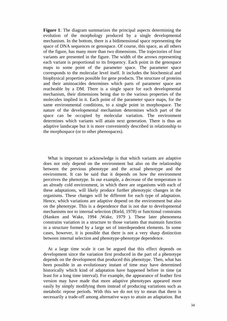
Figure 1: The diagram summarizes the principal aspects determining the evolution of the morphology produced by a single developmental mechanism. In the bottom, there is a bidimensional space representing the space of DNA sequences or genospace. Of course, this space, as all others of the figure, has many more than two dimensions. The trajectories of four variants are presented in the figure. The width of the arrows representing each variant is proportional to its frequency. Each point in the genospace maps to some point of the parameter space. The parameter space corresponds to the molecular level itself. It includes the biochemical and biophysical properties possible for gene products. The structure of proteins and their aminoacides determines which parts of parameter space are reacheable by a DM. There is a single space for each developmental mechanism, their dimensions being due to the various properties of the molecules implied in it. Each point of the parameter space maps, for the same environmental conditions, to a single point in morphospace. The nature of the developmental mechanism determines which part of the space can be occupied by molecular variation. The environment determines which variants will attain next generation. There is thus an adaptive landscape but it is more conveniently described in relationship to the morphospace (or to other phenospaces).

What is important to acknowledge is that which variants are adaptive does not only depend on the environment but also on the relationship between the previous phenotype and the actual phenotype and the environment. It can be said that it depends on how the environment perceives the phenotype. In our example, a decrease of the temperature in an already cold environment, in which there are organisms with each of these adaptations, will likely produce further phenotypic changes in the organisms. These changes will be different for each type of adaptation. Hence, which variations are adaptive depend on the environment but also on the phenotype. This is a dependence that is not due to developmental mechanisms nor to internal selection (Rield, 1978) or functional constrains (Hanken and Wake, 1994 ;Wake, 1979 ). These later phenomena constrains variation in a structure to those variants that maintain function in a structure formed by a large set of interdependent elements. In some cases, however, it is possible that there is not a very sharp distinction between internal selection and phenotype-phenotype dependence. At a large time scale it can be argued that this effect depends on development since the variation first produced in the part of a phenotype depends on the development that produced this phenotype. Then, what has been possible in an evolutionary instant of time may have determined historically which kind of adaptation have happened before in time (at least for a long time interval). For example, the appearance of feather first version may have made that more adaptive phenotypes appeared more easily by simply modifying them instead of producing variations such as metabolic repose periods. With this we do not try to mean that there is necessarily a trade-off among alternative ways to attain an adaptation. But

35

the existence of an adapted part of the phenotype favors the selection of some variants (in the same part of the phenotype or in another part of the phenotype) and may also impose negative selection (mediated through the environment) over other variations (in the case of feathers it is unlikely to develop the making of dens for adapting to cold once feathers have started to develop (in fact birds do not use to dig)). In a sense, although there might be possible to establish a priori the more adaptive phenotype in an environment, the niche available deforms when the phenotype changes. Hence, which phenotypic variants are selected depends on the environment but also in the rest of (and previous) phenotype. 1.3.4 internal structure: levels of organization Leveled system: Systems in which complexity can be defined (as in section 2.2.2) because there is a criteria for defining what is an element, which are the states and which is the linkage. Hierarchic leveled system: Leveled system in which the states of elements are defined by its composition in elements of another type (with its concrete states and linkage). The system has thus two criteria for defining what is an element, which are the states and which the linkage. The system under a concrete criterion A is called the system at level A. Each criterion is called level. The level in which elements are defined by its composition in elements of the other level (or by the linkage of these) is said to be superior to the other level (that is then inferior). Operative Hierarchic leveled system (OHLS): Hierarchic leveled system in which, at least in one level, there are interactions between elements that can change the states of interacting elements. By interaction we mean the physical contact between at least two elements. In addition, the elements of this level can at least make or trigger the first two of these five things (that we will call developmental functions): change of state due to interaction, interact with another element, move (passively or actively), destroy an element (giving rise to its constituent element at some inferior level), generate a new element (from some elements at some inferior level). In the interactions, there are two aspects to consider. One is the specificity (with which elements can an element interact and how likely) and the other is the transformation (response) that an element makes due to the interaction. Both aspects are determined by the composition of the element at the inferior level (or by the linkage of these at the inferior level). This does not mean that it is easy to deduce from their constitution the specificity and transformations allowed by an element. In fact, these elements, because of these properties, are able to make at least simple computations. We will call the network of the system to the set of specificities and responses of the possible interactions among the elements of the system. 1.3.5 Developmental mechanism: During development the zygote transforms into the adult by using the information present in the genotype and zygotic phenotype (and in many

36

cases some environmental cues). The variants that an organism can produce depend on how mutations affect the developmental process and, thus, development itself is one of the most evolutionary important aspects of the internal structure of organisms. In this section we try to introduce as clearly and precise as possible some of the concepts we will require later. Developmental pattern or pattern: is the distribution of cells and their states over space in an embryo or part of it. Form: is the distribution of cells over space in an embryo or part of it (without considering their states). Territory: is a connected group of cells with the same state. In the case that they are said to have the same state because they express a gene in common the territory is called genetic territory. Territories have a form. The embryo can be described as a Hierarchic leveled system in which cell states are defined by its molecular composition. As we already indicated, development is a process by which the information present in the genotype and in the phenotype of the zygote is used to make the complex phenotype of the adult. One of the more apparent phenomena during development is the huge increase in phenotypic information. It starts from a single cell and ends with a complex organism consisting of a large number of cells with different states arranged in a complex spatial distribution. It may be argued that, since development requires the information present in the genome and zygote phenotype, all the information required for development is already present at the beginning of development. That all the required information is already there does not mean, from our definition of information, that there is no increase in the information present in the system (at least in the phenotype). From what we already know about development it is clear that different patterns (and of different complexity) can be produced by developments involving the same number of genes (and with the same number of relationships between them). Thus there is not an unequivocal relationship between genetic information and phenotypic information. Contrarily, which kind of patterns can be generated from a genetic information depends on the "structure" of development, it is on how genes interact (directly or indirectly through phenotype). It does not imply that all developmental information comes from genes, obviously. The relevant thing about how genes interact is not only the exact mechanisms by which each gene interacts with each other but more importantly the whole topology of the network of gene-gene interactions. As we will see, there are multiple ways to organize such genetic information and they allow different types of patterns with different complexity. In fact, two different ways to establish phenotypic information from genetic information can be compared by the amount of phenotypic information that can be generated from the same amount of genetic information. The information at the phenotypic level and genetic level may not be comparable between them, but ways of making the phenotype can be compared at their respective phenotypic and genetic levels. In this

37

thesis, one of the aims is to identify the main different ways by which phenotypic information arises and which evolutionary implications they have. In a coarse way, development can be described as a process by which the phenotypic information of the embryo is increased until attaining the adult state. For those not comfortable with the information concept, development can be understood as a process leading to spatial change. This process can be subdivided into discrete time intervals (that we will call developmental stages or simply stages) in which the embryo, or part of it, changes from an original pattern (that in relative terms we will call prepattern) to a final pattern. Developmental mechanism (DM): A developmental mechanism is the set of interactions and responses to such interactions that are responsible for the generation of a pattern from a previous pattern. A DM is thus a network of elements (they can be gene products or cells; thus a DM can be defined at the cellular or gene level) that interact between them, and the responses that each element have to such interactions. A DM is thus also a network. In order to be a DM this network has to be able to generate a pattern. This implies that if the DM is defined at the molecular level some of the molecules need to mediate a cellular developmental function. From the definition of OHLS it is clear that cells can be considered OHLS (cells being the superior level and intracellular molecules the inferior). Cellular developmental functions include: mitosis, apoptosis, differentiation, cell movement (being it only change in shape or whole cell movement) and interaction between cells. All this cellular developmental functions, as defined in OHLS, are mediated through lower level elements (it is, molecules). Thus mitosis, apoptosis and differentiation require concrete cascades of molecular signals (at least currently, although originally some of them may have been intrinsic to the material basis of the cellular level and not regulated by gene products (Newman, 1990, 1994)). Cell movements and shape depend on the adhesion properties lend by membrane-attached molecules. And, of course, cell interactions are mediated through secreted or membrane-attached signaling molecules. We will classify cellular developmental functions in two types. Those that mediate cell communication, that we will call functions of change of state and those that do not, that we will call functions of change of form or morphogenetic. In a similar way, DMs can sometimes be dissected into two types of smaller submechanisms that can make use of only functions of change of state or of functions of change of form. In such cases we speak of mechanisms of state or state mechanisms and mechanisms of form, form mechanisms or morphogenetic mechanisms. Thus, a DM is a network with the responses to all the interactions specified (it includes the cellular and genetic developmental functions). In order to be a DM it is necessary that the putative DM is causally responsible for the formation of a pattern. Causality implies not only that all the elements, interactions and responses of the DM are strictly

38

necessary for the generation of a pattern but also that some of the elements, interactions or responses of the DM is responsible of the production of some pattern or another of those that the DM can produce. In other words, a correct understanding and testing of the causality of a certain DM in the formation of a pattern implies that the other patterns that such DM can produce need also to be predictable. It can be said that an hypothetical DM can be considered a DM when their variational properties can be correctly predicted. Variational properties of a DM: The variational properties of a DM are a set of properties of the set of different patterns that can be produced by a DM when the following conditions change: 1. w changes: In DMs, elements interact through binding with some

affinity. This can reflect the internal characteristics of the elements that determine the chance that an element interacts with another when they are into contact. It can also be the efficiency with which an element activates or inhibits some developmental function. We will call w changes to the changes that affect such affinities without affecting any other aspect of the DM. These changes correspond, at the molecular level, to mutations affecting a coding or regulatory sequence in such a way that the topology, responses and developmental functions used in the system remain the same (the DM remains the same although mutations of this kind). This category is to some extent arbitrary since some w changes can produce that some interactions never take place in practice. These cases need to be excluded from this category because they really change the DM itself.

2. Initial conditions: Different pre-patterns can produce different patterns for the same DM.

3. Environmental conditions: Environmental conditions can affect development in many cases. These effects are equivalent to transient effects on w or to effects on other aspects of the DM, such as which genes interact among them, etc..

To predict these variational properties is a good demonstration that the proposed mechanism is the cause of a concrete pattern. A more simple demonstration, consisting in showing which elements of a DM are strictly necessary for the formation of a pattern, is not fully satisfactory since it does not discriminate between elements that are simply required and elements that explain variation. Lets us propose an example for this that also highlights some problems of current thinking in developmental biology. Let us assume that a DM generates pattern in a group of cells by (among other things) the secretion of multiple signaling molecules over extra-cellular space. In this case, any gene involved in the exocitosis of the signaling molecules, that when is mutated simply does not allow it (but its effect is all or none), can be said to be required for the formation of the patterns that the DM is suppose to make. However, this gene cannot be said to have a causal role in the formation of the pattern because its variation would probably only affect that a pattern forms or not but it does not explain why the pattern is the way it is. In general, a causal explanation is unlikely to reside in a single gene but it has to deal with

39

how many genes coordinate each other behaviour and the behaviour of cells over space and time, in other words in DM functioning and topology.

1.4 E-C paradox: Once the basic principle of evolution and the leading forces acting on evolution have been presented and described in some broad way, it is time to present in a coarse way how these forces and general principles acting at each time in evolution can be used to predict how evolution will proceed in a lineage through large intervals of time. In order to make predictions, and understand, what is taking place in evolution it is necessary not only to identify the acting forces but also to see how they can interrelate with each other in the course of time. We will suggest that this close interdependence among these three forces produces that any of them can be understood to some extent without a corresponding understanding of the others. This justifies the requirement for the new kind of approach that we will use here. Development is a "product" of evolution (and then, to some considerable extent, also a product of selection). It implies that the DM that each individual in an evolutionary time instant has is not necessarily the more adequate or logical DM. This is, DMs do not need to be the more optimally adapted to some of the selective pressures that may currently act in the DM itself (like energy cheapness or quickness). In other words, when looking at a developmental problem, as "which is the mechanism implicated in the formation of this pattern", it may not be the case that the more simple or economic (or whatever criteria a researcher may use) DM imaginable and possible is the one actually used by the developmental system under study. This is because what is presently found depends in complex ways on which have been the selective pressures acting over time on the variations that have been produced in this organism lineage. This leads to acknowledge that to understand development in a lineage it is required to understand its evolution, and thus the dynamics of the evolutionary process itself. Of course, development can be understood by crude experimental force without any evolutionarily-based hypothesis. But this way we can understand how things work but not why. In addition, and as we will later show, by doing this we are missing a big bunch of information that can allow to understand development with less experimental effort. This is especially true if a large part of available experimental information is scattered over diverse and disparate phylogenetic groups, as is the case in developmental biology, and/or if we try to understand development in many groups. On the other hand evolution can not be understood without understanding development because at each evolutionary instant which variations can appear depends on the existing DMs. And, of course, what development produces is independent of what selection selects for (this does not apply to past selection since past selection can have affected how development is, although not directly).

40

In summary, to understand evolution it is needed to understand development and to understand development it is needed to understand evolution. This produces an apparent paradox, an “egg-chicken” paradox. In the following section we will try to show how this paradox can be solved and used to cast useful and testable inferences about both how evolution is and how development is. This would be consistent with how we think a more satisfactory evolutionary theory has to be. It has to be able to make predictions about how and why organisms change and thus has to be able to make predictions about organisms structure at various time intervals.

41

1.5 Objectives: 1. To study which is the capacity of variation that developmental

mechanisms have. 2. To determine if developmental mechanisms can be categorized into a

limited number of types sharing variational properties and structural properties.

3. To evaluate the variational properties of the different types of developmental mechanisms.

4. To elaborate a theoretical framework in which some understanding of which variation can be produced by different types of developmental mechanisms can be integrated with what is know about selection and history in order to make experimentally testable predictions about how morphology and development evolve.

5. To evaluate which kind of predictions about the structure of development can be made in the case that there is a limited number of types of mechanisms.

6. To evaluate how the interdependence between development and evolution can change the spatiotemproal context in which evolutionary inferences can be made

To evaluate to which extent the predictions made for development can be useful or orientative for other kind of phenomena.

42

2. Methods : This thesis is composed of various different works related by an underlying theoretical framework. This framework includes a methodological approach to the questions we have presented in the introduction. This framework will be presented here. Later, in the results, we present the methodology used in each of the models we have developed. In this methods section we describe some aspects of the developed theoretical framework and some problems related to it. In essence thus, we describe here the kind of reasoning we will use to solve the problems we point in the introduction.

2.1 Theories of the origin of information:

The theoretical framework presented here is based in the assumption that all the possible DMs by using the known developmental functions at the cellular and molecular levels, can be categorized in a limited number of types. These types are supposed to be definable by some structural characteristics and at the same time need to have dramatically different variational properties (and other evolutionarily interesting properties) . By structural characteristics of a DM we mean, for example some aspect of how is, for example its topology, the kind of developmental functions it uses, etc... In a later section we will try to show which is the evidence for the finiteness of such types. We will also discuss to which extent this methodology can be applicable to all living systems but, unless explicitly stated, we will restrict the work to metazoan. We use the name, theories of the origin of information because the following reasonings come from assuming that there is a limited number of types of DMs able to increase complexity in the phenotype. In addition, these types correspond, in part, to the different proposals that exist in the literature about the functioning of development. 2.1.1 Theories of the origin of information: Evolutionarily interesting properties of a DM: Let us assume we have a population in an environment in which a morphological transition has taken place recently in some part of the phenotype, at least in one individual. Let us assume too that this transition is produced by the involvement of a new DM at not by some change (like

43

a w, prepattern or environmental change) in a DM already acting in this part of the phenotype. A simple clear example could be a piece of skin spatially homogeneous in which some spatially heterogeneous morphological prepattern has recently appeared. The following can also apply if what has happened is that an already existing DM has been recruited in this part of the body or if a DM acting in this part of the phenotype has changed in such a way that it can no longer be considered as the same DM. One of the questions that we will like to address in this thesis is if we can know which type of mechanism is more likely involved in the formation of this variant. There are various aspects of a DM that are useful for addressing this question. 1. Properties of generation of a DM: Here we include structural properties of a DM that can be related to the likelihood with which a DM can be generated de novo or from an already existing DM by variation at the molecular level. It can be assumed to be roughly proportional to the number of molecules and interactions between them implicated in a DM. Hence, these properties are related to the DM at the molecular level and can be taken as a way to estimate the probability by which such DM may appear to be involved in the development of a pattern. 2. Variational properties of a DM: we already explained this concept but here it is interesting to introduce some aspect of them that are specially important: a) Number of different patterns that can be produced b) How different are the patterns produced. These two categories can be joint in a simple one referred to the theoretical morphospace available by the DM. The morphospace is a space in which he patterns produced by a DM can be spatially ordered in function of their similarity. Its analysis allows to grasp evolutionarily interesting information like: - The space reachable by a DM. That is, essentially, the number of patterns attainable (Through w mutations, prepattern changes and environmental changes). - The distance among near patterns in the morphospace. That is how different and how spaced patterns are. - How many neighbor patterns a concrete patterns has. - The form of the morphospace itself. c) How complex are the patterns d) How homeostatic are the patterns to external transient perturbations.

44

3. Relational properties between the genotype and phenotype: This relates mainly to how complex is the relationship between phenotype and genotype. It can be that two patterns are very similar but that the DM producing them has very different w values (and then it can be said that they are molecularly quite different, although remaining as the same mechanism, so they are two networks of the same mechanism). It can also be that in different DMs a small mutational change gives rise to phenotypes considerably different from the wild type phenotype (in such case we will say that there is a complex relationship between genotype and phenotype). 2.1.2 Theories of the origin of the information: potential predictions: If it is true that all possible DMs can be categorized in a limited number of types with identifiable similar structural and evolutionarily interesting properties, and if these types and properties can be studied, then, as development would be describable in terms of which types of DMs are used in each development, many powerful predictions about evolution and development are possible. These are: 1. Structure of the phenotype and development: What will be predictable depends on the amount of information available in the system (specially about its history). But, in many cases, the relative frequencies of each type of DM in a concrete development would be predictable. It also allows to predict the relative frequencies of types of DMs in different stages in development and from this have some picture about how development is organized in different stages. Equally, the frequency of apparition of each type of DM in different evolutionary contexts is also predictable. 2. Predict the variational properties of present and past organisms. From this framework it can be possible to predict which kind of phenotypic variation a lineage will exhibit. 3. Phylogenetic patterns: The predictions of the variational properties may allow, in some cases, to predict in phylogenies, how different are species in the same lineage in relationship to their divergence time from their last common ancestor. Moreover, other properties about how disparity is distributed in a phylogeny are possible. In this thesis we will try to show how all this is possible. We will also present some examples of the application of these predictions on some experimental systems. At the same time we will present how the general application of this methodology can give useful insights about how evolution has taken place. In the discussion, we will present how these predictions fit what is known about evolution and development. 2.1.3 Theories of the genesis of information: types of mechanisms in metazoan: In this section we present some aspects of living beings structure that suggest why there may be a limited number of types of DMs and under

45

which criteria can metazoan be considered OHLS. A level of organization that receives considerable attention in current developmental biology is the molecular level: 2.1.3.1 Molecular level: The organic molecules implicated in life can do only three things at the molecular level. Often researchers speak about complex gene functions but it can only be said when looking at the effects of a gene in an upper level (being it morphology or other), so they can be described as effects and not as functions. In addition, in most cases such effects depend on many things, such as the epigenetic context, and its use is confusing and, in a sense counterproductive. Strictly, molecules can only do three things: they can bind (transiently or more permanently) in a more or less specific way to other molecules. React, due to binding, with other molecules, giving thus rise to other molecules. They can move, being it passively through diffusion or actively as is the case of some protein complexes like some of those using myosin and kinesin. Movement can be internal and thus can give rise to a change of state of the molecule (a conformational change as those that often take place in many proteins). Living beings can be described as OHLS at this level. The state of their elements, the molecules, can be defined by their composition from elements of a lower level, the atomic level, and/or from the linkage that the elements of this lower level have in an upper level element. A change of state includes thus chemical transformation of molecules through reaction or simple conformational changes without reaction as those that often occur in proteins after interaction. These three things are the molecular developmental functions of current living beings. A molecule may be able to produce the formation of another molecule from their atomic constituents and also degrade molecules to their atomic constituents. Hence, it can be said that there are five instead of three molecular developmental functions. In some cases, molecules can have simple computation capabilities. It happens often in proteins in which the function (for example to which other molecules a protein can interact (or the affinity of such interaction)) is state-dependent and multiple states are possible (transitions between states depend on previous states and on the interaction). Actually, even the set of possible reactions in biological chemistry is relatively small. These reactions are mainly those that the functional groups of organic molecules allow. In fact, the large amount of molecular diversity found in living systems is more a consequence of the diversity of molecular arrangements of atoms than of the diversity of atoms implicated. In biological chemistry what is normally important is the "form" of the molecules. An example of this is that proteins are composed of only twenty aminoacids and catalyse a large number of reactions only by specifically binding reactives and positioning them adequately in order to increase the chances of concrete stereoreactions. All development is based on molecules doing these three things and affecting cellular developmental functions. Strictly all developmental processes can be described as a concrete spatio-temporal sequence of interactions between molecules. This is because the cellular level and other

46

possible upper levels are formed by the lower levels plus space (or linkage). It does not imply, however, that the molecular level is the more adequate for understanding development; and as we will try to show, in many cases developmental processes have to be seen at two levels at the same time. 2.1.3.2 Cellular level: Cells, under an appropriate criterion, are also OHLS. Cells are composed of molecules with concrete spatial relationships between them. The state of a cell can be defined by the composition and linkage of their lower level elements, the molecules. In fact, a differentiated cell is characterized by the expression of concrete gene products and by its form. Cell form, in fact, implies concrete spatial distributions among molecules (for example of the microtubules and substrate-binding membrane molecules). Cells can also do a limited number of things. These cellular developmental functions are: Cells can interact with other cells (through the secretion and receptions of molecules) and change of state due to this interaction. Cells can produce other cells (mitosis). Cells can also undergo apoptosis. Cells can move, actively or passively, and as a consequence of such moving they can change its shape ( we note that both active movement of the whole cell and movement of only part of the cell leading to shape changes are mediated by binding of molecules on the membrane of the cell to the extracellular environment (that may include other cells)). Cells can also compute. The change of state that a cell will undergo after an interaction depends on the signaling molecule received and on the previous state of the cell. As in the case of the molecular level, all the development can be described as a concrete spatio-temporal sequence of cell interactions and responses to these. In fact, the molecular level can be ignored by simply tabulating which response a cell will have when receiving a concrete signaling molecule and being in a concrete state. In a sense, the molecular level can be seen as the immediate cause and mediator of the cellular developmental functions and of this table of interaction responses. But if the table is known, there is not necessarily any advantage in knowing how these cellular developmental functions are performed at the molecular level since development consists in an increase in phenotypic complexity. In fact, relevant things in development happen at the cellular and superior levels. However, the molecular level is closer to the hereditary information, and thus really matters from and evolutionary perspective. For example this internal table is indirectly encoded in the genome and in order to understand how it can change it is necessary to understand how it works at the molecular level. 2.1.4 A classical description of development: The two previous sections seem to point that both molecules and cells can do a limited number of functions. This suggest that development diversity arises from how this limited number of developmental functions

47

is spatially and temporally coordinated in adequate networks. This is more important than differences in the number or types of developmental functions used or in some special characteristics of some genes. In essence, the importance is on relations rather than on identities. We will later argue why development may work this way. Although the amount of experimental ( and consequently economic) effort devoted to the study of development is considerable (specially at the molecular level), there are not many studies trying to grasp general results or metaphors about how development works. This can be due to the eminently empiricist tradition of the field (at least in the last few decades) but also to a considerable belief in the reductive capacity of genes (in a similar way as what we have suggested that happen in the neo-Darwinian synthesis). Many researchers, a part from layman, think more or less implicitly that genes can really directly control by themselves complex functions at levels upper to the molecular. This perception is clearly affected by the impressive phenotypic effects that some mutations can have (and the consequent effort in the promising area of expecting to found a close correspondence between a gene and a phenotype). Many years ago two experimental developmental biologists explicitly stated their views about how developmental biology has to proceed. Needham (Needham, 1933) argued that general theories about how development works are required in order to integrate existing experimental data and guide further experiments. He also argued that simulation and modeling would be a useful tool to see the implications of the theories. Another view (Spemann, 1938) suggested that no theories are needed because how development operates would become evident once enough information has accumulated. The metaphor was that developmental biologists are as archeologists that reconstruct a broken amphora from their pieces without having any idea about the global shape of the amphora. Since then, and in spite of recent claims for a more needhamian approach to development (Gilbert and Sarkar, 2000), most research in developmental biology has followed this Spemann view. In our view this has produced that, although a huge amount of experimental data has been attained, development itself is still poorly understood. Prove of this is that how patterns are causally formed is only known for very few systems. An additional prove is that there are few studies trying to outline a general picture about how development may work. In this section we will briefly summarize them and explain why some of them may not be very useful. In general, the studies trying to extract general features of development are restricted to look at how genes interact to each other over time. So, as in the case of neo-Darwinian synthesis, in which evolution was reduced to look at how gene frequencies change over time, in development the reduction consist in looking to how gene (expression) changes over time. In this case, however, there is more interest in gene interactions (at least at the molecular level). Hence, a very hierarchic view by which a limited number of genes (master genes) were supposed to completely specify the phenotypes of

48

large parts of the body by activating a hierarchic cascade of downstream genes sequentially (each responsible of the phenotype of a more limited part of the body) is still implicitly taken as close to what may be happening (Levine and Harding, 1987). Later authors have developed more fine descriptions of how this may take place. Many researchers do not think on master genes directly determining the phenotype of some parts of the body. First, they experimentally show that some of these putative master genes can act at different levels of the “hierarchy” (Akam, 1998). Others also show that some of the “decisions” made by such genes are not really determinative and can be circumvented by other compensating effects of downstream genes (Gibson et al., 1999) or , contrarily, they require some posterior and likely independent determination event (Castelli-Gair, 1998, Weatherbee, et al., 1998). Some of the general statements cast in these studies are likely to be true, at least at some level. For example, many evidences point out that development proceeds by making first large determinations of fate in large areas of the embryo by later, based in these first events, going into more close fate details in more spatially restricted parts of the embryo. Many developmental studies are devoted to study the role of some gene in the formation or determination of some pattern. But what really means that a gene determines or patterns some part of the embryo. Strictly, when it is said it is because, normally, it has been shown that when this part of the embryo is allowed to develop in isolation it develops normally (although the criteria for saying that this development is normal may be discussible in some cases). The relevance of this is relative, and in many cases depends on which is the implicit idea about how development works that the researchers have. But for sure it can only be said that this gene is required for the development of such part of the embryo and that actually the development of this part of the embryo seems to be independent from the rest of the embryo. It does not necessarily imply, and it is probably inappropriate to think this way, that such gene is controlling all the process (of the formation of such structure) or that it has the information for making it. In fact, to know that a (or many) gene(s) is(are) necessary for a process is and advance, but it does not aid too much to know how a pattern develops. For this goal, we need to know how cell states are spatially (so spatial distributions, it is pattern itself, has to be explained) determined in this part of the embryo and how genes coordinate the cellular processes that need to take place most of the time during which this structure is developing. Since development is spatio-temporal coordination of cellular behaviours, what is needed is to understand how genes interact with each other and with cellular behaviours in order to attain the adequate patterning. There are some implicit assumptions used by many developmental biologists that minimize the importance of understanding this coordination. Usually, no attention is paid to space, pattern formation and morphogenesis (specially as a process in which what has to be understood

49

mainly is the spatio-temporal coordination). In many cases, much attention is devoted to disentangle the whole chain of molecular interactions required for correct development. One implicit assumption is that knowing the molecular details of the interactions that need to take place it can be understood how pattern formation takes place. As we noted in section 1.3 this is simply insufficient to consider that something has been understood about pattern formation. In addition even in the context of hierarchic chains to know how each molecular interaction takes place does not explain how the chain behaves. The other assumption is that genes interact through hierarchic chains that produce things at a macroscopic level, for example patterns. In some cases, these chains are described as networks, although normally they are supposed to be hierarchic. The main problem is, however, to think that development can be understood by looking at what happens inside cells. Wolpert’s (Wolpert, 1994,1989,1981,1969) work is one of these explicitly stating this widespread view. In the most extreme version of this view the idea is that each cell, due to the expression of some genes, undergoes some kind of unique genetic program that allows each single cell to individually coordinate all the processes that need to be fulfilled for a correct development. Each cell has a different genetic program and the individual reading of such program allows the correct development of a structure composed of many cells. Coordination is thus a by-product of the independent action of cells following its own genetic program (Wolpert, 1969). The main experimental data that is supposed to support this view consists on mutants of some transcriptional factors. In these mutants, some cells (normally those expressing the transcriptional factor, but frequently others too) do not develop correctly, in some cases in a way that depends on the degree of expression of the gene in the mutant. Since these effects use to happen from the developmental stage at which the mutated gene is first expressed, this view interprets these results as showing that this transcriptional factors guide the development of the cells expressing them during development. In a sense, the transcriptional factor should say to the cell (by activating the adequate genes at each time) what it has to do at each time (Wolpert, 1989 ). The current understanding of development can be argued to be insufficient to discard some hypothesis but the previous view is misleading, at least in its more extreme version. The reasons are multiple; first the supposed experimental foundation of this view offers other more plausible alternatives. Second, a large amount of experimental evidence argues against this view. Third, this view has many experimentally unsupported implications that are not stated even by the former proposers. Fourth, it has many internal inconsistencies. Fifth, it is unlikely that evolution has generated such an improbable way to operate. That a transcriptional factor is required for the correct development of a group of cells does not mean that its effect is independent of the rest of the cells. In general, cells are constantly sending signaling molecules between them. That a part of the embryo can develop independently from the rest (even if it is because it can express the transcriptional factor) does not

50

mean that these cells are simply following an internal developmental program that this transcriptional factor (or a combination of others) determines. It can be the case that these cells (an because they express this transcriptional factor) are sending signaling molecules to their neighbours (even to those that are expressing also the transcriptional factor) and that this signaling is also required for the correct patterning of this autonomous part of the embryo. So this “genetic program” can include among their instructions the sending of signals. In fact, such signaling can affect cells expressing the transcriptional factor in such a way that it can affect what this cell is going to do next. Hence, such genetic program may be affectable by the recurrent and constant signaling that cells use to have and, in fact, it can be the case that the program is not only affectable but, in fact, requires this constant signaling. Signaling can also affect the morphogenetic processes that cells are constantly undergoing (processes that, as we will see, necessarily imply, in many cases, a mechanic coupling between cells), thus, it can affect the spatial localization (inside this independently developing part of the embryo) of the cells that will send a signal (and, thus, the spatial localization of the receivers). The important thing is that the original wolpertian view and this view, in which a group of cells expressing the transcriptional factor control the autonomous development of a part of the embryo by coordinating what cells do by signaling and by how cells behave, will give the same experimental results (so a different kind of experiment is required in these cases). Then, it can be said that this experimental evidence is not sufficient. My impression is that in the cases that such view is advocated the evidence is scarce, since it can be interpreted in other ways that seem more plausible from what we know cells do (but quite often what a researcher expects to see conditions how he would perceive the results). Another problem with this widespread view is that it is not very explicit and consistent in what it tries to show. An important claim it makes, that is normally not taken into account, because it is strongly embedded in main developmental biology, is that pattern formation and morphogenesis are considerably independent (Wolpert, 1989; Bart, 1990). Concretely, pattern formation is assumed to take place first and morphogenesis later, depending on how pattern formation has taken place before. In this case, even the terminology used is considerably biased. The word pattern and the concept pattern formation implicitly assumes this relationship between pattern formation and morphogenesis, in fact, it has in its body some kind of molecular preformationism. Originally, a pattern is some kind of visual guide, like a coarse-grain view of a picture used by a tailor in order to, later, more finely make a fine wear. Pattern formation stands mainly for the determination of concrete fates to cells. That it happens in space is implicit but not always has gained too much attention. In some cases, the word patterning is not even used in a spatial context. It is interesting to note that the positional information view was developed in a time where developmental genetics were still very underdeveloped. This positional information view is not really consistent with what cells do at the molecular level, as we will show, and can be historically considered a metaphor to interpret the results of early experiments.

51

The wolpertian view proposes that some early patterning event (the existence of gradients of signaling molecules) produces the setting of different genetic programs in the cells (depending on the received concentration of these molecules). Then, morphogenesis takes place more or less independently in each cell by following a different genetic programs. The works exposing this view do not explain if this is supposed to take place only once (something unacceptable for almost any developmental biologist) or happens many times through the course of development (and thus such genetic programs may be reinterpreted by cells). In any case, however, it seems that morphogenesis is dependent on pattern formation and does not affect pattern formation itself. With some exceptions (see below), during development, morphogenetic changes and pattern formation take place at the same time. Many researchers (Lovtrup, 1984) consider that early development consists mainly in pattern formation while later development consists mainly in differential growth and morphogenetic events. Although this view can be seen as a coarse but correct view of development, it is not very useful to understand how phenotypic complexity increases in development. Morphogenetic processes are more important than patterning ones during late development but the reciprocal is not necessarily true. In fact, even if there are few morphogenetic changes when patterning is taking place, the few there are, can be very important because they affect where inductions are taking place (because they can affect the relative positions of the cells that send signaling molecules and the cells that can potentially receive these signals). In any case the truth is that there is not evidence to suppose that pattern formation and morphogenesis are independent, contrarily, looking at when both processes are taking place it seems likely that both processes affect each other, although there are few articles studying experimentally this possibility. In fact, as we will later explain, morphology (during development and later as the product of development) and space itself are aspects that do not receive too much attention by most developmental biologists, even if a large part of the development process complexity is in the complex morphologic changes that take place. Why the wolpertian view is very improbable evolutionarily will be explained in more detail later. This view is interesting because, although unrealistic, describes an extreme case useful for ideal comparisons. For the moment, it is interesting to note that, as each cell needs to make all the fine changes required to form adequately a part of the adult structure, each cell needs a very precise program (and thus many genetic information). 2.2.2 An actualised description of development. In this section we will present a general view of what we think is going on at the cellular and molecular level during development. Later we will show how this view is possble and consistent and how it applies to some example developmental systems. During development, cells are constantly sending molecular signals to each other. It is actually known that the signaling molecules used by most metazoan are very similar and that they can be grouped in a relatively small number of molecular families. In a similar way, the transcriptional factors used in metazoan development are

52

also considerably conserved, although probably not to the same extent. Signal transduction pathways exhibit also a considerable degree of conservation. This suggests that the extraordinary morphological disparity that metazoa have attained is due more to how these are related to each other and, probably to the cellular behaviours (cellular developmental functions), than to the exact molecular identity of each gene. Thus, the disparity appears from how development is organized (this is its architecture) rather than from the exact nature of its minimal functional elements (it is molecules). Of course, the development is due to (among other things) the genes, but it is caused in a so indirect way that the nature of the genes themselves may not be very informative if it is not joined with other kinds of information. It has been often observed that signaling is crucial for correct development. When looking at which are the effects of the reception of a signal by a cell, it has been often found that they activate signal transduction pathways, that lead to the expression of concrete sets of transcriptional factors (Barlow et al., 1999; Bushdid et al., 2001; Bang et al., 1999; Bei and Maas, 1998; Niswander and Martin, 1993). Which transcriptional factors will be activated depends not only on the signal received but also on the previous history of the cell (Goumans and Mummery, 2000). This history consists mainly in which transcriptional factors and signal transduction pathways molecules a cell express (among other aspects related to this, like the condensation and local topology of DNA or the concentration of signaling molecules or ions in the cytoplasm). Transcriptional factors affect cell behaviour indirectly through the activation of other transcriptional factors or/and by activating the expression of molecules involved in mediating cell behaviours. Hence, it has been found that cells respond to signaling molecules by, indirectly through transcriptional factors that integrate response with previous history(Goumans and Mummery, 2000), altering its cell behaviours. For example, by undergoing cell division(Hu et al., 2001; Cecchi et al., 2000; Park et al., 1998; Salser and Kenyon, 1996), apoptosis (Su et al, 2001; Barlow et al., 1999; Ferrari et al., 1998), shape changes mediated by the alteration of the adhesive properties of the cell(Wacker et al., 2000; Lincecum, 1998; Packer et al., 1997; Jones et al., 1992), migration (Herman, 2001; Houzelstein et al., 2000; LaBonne and Bronner-Fraser, 2000; Epstein et al., 2000), expression of concrete signaling molecule receptors (Panchision et al., 2001; McPherson et al.2000) and secreting the same or different signaling molecules(Montross and McCrea 2000; Carnac et al., 1996). It is interesting to note that cells actually compute. Inside the cell, the network of interactions between expressed transcriptional factors determines which will be the effect that the receiving of an external signal will have. Thus, the genetic program metaphor does not seem to be adequate. Instead, what cells do is to receive signals and then read its internal state and integrate both informations to undergo a concrete response. A more useful metaphor would be that cells have some kind of internal table that they use to specify which response they have to undergo when they receive a signal and have some transcriptional factors expressed in them. Of course, this table is the network of transcriptional factors and signal transduction pathway genes,

53

that depends on the characteristics (molecular developmental functions) of these genes, that are indirectly determined by the genome. This table is relatively simple, with few inputs (signaling molecules) and few outputs (cellular developmental functions). Hence, in order to understand development, it is needed to understand what happens inside cells under different extracellular circumstances but also to understand at each moment how cell behaviours affect the spatial distribution of cell states over space. From this perspective, development seems more to be a collective phenomena of cells communicating to each other, in which a correct spatio-temporal coordination of cellular events is accomplished through the dynamics of signaling, its effect over the cellular behaviours and the topology of the internal gene network topology of the cells. In this thesis we precisely explore the different ways by which this collective process can take place, so which types of DM are possible.

Results: Introduction to results In the results we present some of the articles published, submitted and in preparation that have appeared from the work of Isaac Salazar Ciudad during his thesis. Each chapter corresponds to a paper or related set of results. In addition, we include some justification of why we have taken these approaches in each case, in special reference to how they relate to the main theoretical framework we try to develop.

3.Systems with only cell communication: Gene networks capable of pattern formation: 3.1 Introduction: In the literature devoted to the study of development, how pattern formation takes place is a question that is not often addressed directly. This may be due, in part, to the fact that in most developmental systems under study there is not enough knowledge of the system as to address these questions. Another reason may be that researchers are very interested in looking to the effects that a simple gene can have on the phenotype and

54

are not so concerned with understanding the topologies of the networks or how cellular developmental functions are coordinated. Probably, this happens due to Spemann-like views that assume that a single gene can explain a lot or that the identification of the effects of many genes as possible is the better (or the currently most possible) way to understand development. However, there are many studies that try to see the effects of the signaling by some molecules over patterning processes. These usually deal with one or few types of molecules and do not consider other cell behaviours than signaling. In a limited number of systems such approach, when undertaken by multiple genes, has been able to outline a considerably clear picture about how patterning takes place, and hence about how is the DM that gives rise to a pattern. Unfortunately, such systems are systems in which only one cellular developmental function is used. This is actually not a coincidence because they are more easy to understand. In general, as morphogenesis is supposed to take place after and subordinately to pattern formation, an effort to understand the complex dynamics of systems undergoing morphogenetic changes while signaling is taking place has not been undertaken. As we will later argue, patterns that arise only from cell communication are not very common. But, since they are the most easy to understand and the ones for which there are more information, part of this thesis is devoted to them. Examples are frequent in very early development. These include the segmentation of Drosophila (Gilbert, 2000) , the determination of wing veins in Drosophila (Bier, 2000), the notch-delta system (Lewis, 1998), the vulva of Chaeordorhabditis elegans and other nematodes(Wang and Sternberg, 2001) and the cleavage of some echinoids (Davidson et al., 1998) and tunicates (Jeffrey, 2001). Gene networks only including the developmental functions of cell communication are a good and simple starting point to evaluate to what extent there is a limited number of DMs. It is possible that all gene networks capable of pattern formation need to satisfy some topological criteria. In other words, there exist the possibility that there is not an infinite number of ways to make pattern. Moreover, we know that there is a limited number of genes and a limited number of signaling molecules, so the question can be transformed into a more tractable one: with a limited number of genes, is there a limited number of types of mechanisms, or conversely, there is no way to classify mechanisms? This question is impossible to address from a simple evaluation of existing experimental data, since there are few examples in which the gene network responsible of a pattern is known (and in all cases they are gene networks that only include cell communication). In addition, an analysis limited to existing data would be problematic from an evolutionary point of view, because it would be difficult to evaluate whether the kind of networks we found are the only possible or are only a subset of all the possible that have been selected or favored by chance. As we know with some detail how the basic interactions take place at the molecular level, we can theoretically evaluate which networks, made of basic interactions, can give rise to pattern. The important point is to correctly simulate these basic interactions in order to correctly estimate what is really possible. In

55

the first article (see below) we have performed such approach. In this article we actually show that it is really the case that there is a limited number of types of mechanisms. They strongly differ in their topological properties but also in some of the properties of the pattern they produce. For looking the programs used in simulations see annex I. A related paper can be found in annex V. 3.2 The article:

56

4 . Variational properties of systems with only cell communication: 4.1 Introduction: In a second article (see below) we have studied the variational properties of the mechanisms identified in the first article. In the third article (see below) we show some experimental examples of how this kind of analysis can shed some light into concrete problems in evolution and development. For looking the programs used in simulations of section 4.2 see annexes II and III.

4.2 The papers:

57

5 Systems with cellular developmental functions of change of state and of change of form.

5.1 Introduction: The inferences made in the previous section have a limited validity since they are valid in those stages in which pattern is attained by using only cellular developmental functions of change of state. This is not very frequent and, in an evolutionary context, it is even less useful (although as we have seen it can be very useful in some cases) since this type of mechanisms can be substituted by mechanisms using more developmental functions. In such cases it would not be useful to use what we know about emergent and hierarchic mechanisms. The reason is that a mechanism using only signaling to generate pattern can be substituted by a mechanism using more developmental functions. Hence, the emergent-hierarchic dichotomy is useful only in some cases. To discover if there is a limited number of types of DMs (and which are they) that use any cellular developmental function can be a very difficult task. From an experimental perspective there is simply not enough data since there are few cases in which we know how pattern is produced. To simulate gene networks using all possible cellular developmental functions is a hard task since there is no obvious realistic, computationally tractable, way to implement them (and it is not even clear what would be really realistic). It is a task that I plan to do in the future in spite of such considerable difficulties. In this thesis I have adopted a more subtle approach that is also simulable. Although, in general, much more effort has been devoted to DMs using only cell communication, there is also some understanding of DMs that use only mechanisms of form or that are composed of a first submechanism of state and a later submechanism of form. This is the case, for example, in the leg imaginal discs of Drosophila, where a first set of signaling events establishes genetic territories and later the territories unfold through cell shape changes (Serrano and O’Farrell, 1997; Condic et al., 1991) in such a way that a leg-like appendix forms. Normally, these morphogenetic mechanisms are studied in isolation, so developmental biologists look at cell states determination or at morphogenesis, but not at

58

the two things at the same time. If the two things are studied simultaneously, it is often assumed that cell states are determined before and form later. In the following section I will present part of a preliminary paper I am developing with Stuart Newman that tries to summarize all the DMs proposed in the literature for which there is some experimental evidence. They are classified by the types of cellular developmental functions they use and, for this reason, we will call them basic developmental mechanisms. In fact, proposed mechanisms include normally one or two developmental functions only. 5.2 A repertory of developmental mechanisms: 5.2.1 Cell autonomous mechanisms Cell autonomous developmental mechanisms involve a unique cellular developmental function: mitosis. Thus, cells do not interact mechanically or by signaling. Some of these mechanisms can generate pattern from homogeneous prepatterns. The ability to generate pattern from the progeny of a single cell requires that the internal state of the cell becomes non-uniform in space or time. See fig.2. 5.2.1.1. Division of a heterogeneous egg: With few exceptions (mammalian and some turbellarian clades) egg cells have some internal polarities that can be used to differentially bind gene products or mRNAs to different parts of the cell. Non-uniformities in the egg involve some prior interaction with other cells, maternally directly inherited cell polarities or non-uniformities inherent to all the cells. They can come from the embedement, through signaling, of spatial pattern from cells surrounding the oocyte. This seems to be the case in Drosophila (Riechmann and Ephrussi, 2001). In other cases, the oocyte animal-vegetal polarity simply comes from the polarity of their mother cell. The spatial distribution of normal cellular compartments (specially the cytocortex versus the cytoplasm) can also be used to distribute different mRNAs to different parts of the egg. The basic mechanism consist in binding of specific mRNAs to the different compartments existing in the cell (Zhang and King, 1996; Jeffrey, 1985). Then, the symmetric or asymmetric cleavage of the egg causes blastomeres to contain different factors depending on their position (it is depending of which portion of the egg cytoplasm they include).

59

Figure 2. The diagram summarizes the logic of the basic DMs. Asymmetric mitosis. The straight lines represent polarized microtubules in the animal-vegetal direction. The ovoid anchoring proteins. Later, the two mRNAs A and B are distributed to opposite poles of the cytoplasm. Division of an heterogeneous egg: mRNA A is anchored to the animal cytocortex, C mRNA is in the animal cytoplasm while B is in the vegetal part. Division makes that different blastomeres take A, B, C, A and C, and A and B. Internal temporal dynamics coupled to mitosis: The first drawing represents the gene network producing the temporal dynamic. The

60

gene product A is typed as “a” when it is at low concentration and as “A” when it is at high concentration. Cells in bold are cells in which the gene network dynamic is frozen. Normal arrows indicate positive interactions while cut arrows indicate negative interactions. Directed mitosis: The lines represent mitotic microtubules and the black ovoid chromosomes. Black circles are interfase nuclei. The part of the membrane where the cytokinesis ends has some special characteristics of the cytocortex (draw in grey only in one cell). In the second mitosis this area attracts some microtubules making the nucleus to rotate. This rotation also affects the rest of mitosis microtubules and the cytokinesis plane. Differential growth: Areas in black are groups of cells with a different state. They proliferate more quickly than white cells and buckle inward. Apoptosis: The cells in grey are going to undergo apoptosis. After this, the form of the pattern has changed, and thus also the pattern itself. Adhesion: A cells bind more strongly among them than to B and than B to A. This produces that the cells B surround a central core of A cells. In an epithelia some cells have a strong affinity in their basal membranes for the substrate but, their lateral junctions are strong enough to forbid individual cell migration. This produces that this part of the epithelia deforms to maximize their contact with the substratum. Lateral binding among cells produces that it takes place in the form of an epithelial invagination. Contraction: Planar forces stretch an epithelia. Epithelia may behave as only partially elastic material. The material nature of the cells and their bindings make that the epithelia folds or relaxes in a specific way. Migration: Some attractor factor makes a group of cells (in grey) to spread over a wide area. The form of this area is determined by the distribution and form of the tissues that allow the pass of migrating cells (it depends on its material nature and on the presence of adequate binding substrate), by the form of the source of attracting factors and by the number of cells implicated in the migration. Matrix swelling: Two pieces of connective tissue differ in the concentration of cells they have. The right piece, that has more cell concentration, starts to secrete more matrix until reaching the cell density of the other piece. It produces that this piece expands in space.

61

How the compartment destination of a mRNA is determined is not known, but it may involve the binding of mRNAs to anchor proteins associate with microtubules (Kloc and Etkin, 1998; Elisha et al., 1995). In the case that the internal polarities of the cell are intrinsic the DM is strictly autonomous. One reasonable possibility, taking into account what we know about what genes do and about the structure of cells, is simply that which gene products are transported to each place depends on their sequence dependent binding to a limited set of microtubule anchoring proteins. Although the number of genes differentially localized can be large, the number of different spatial localizations inside the cell is small and most of these genes play supporting roles that can be compensated by zygotic transcription. In most metazoa, it seems that there are four compartments. Two correspond to the opposed sides of the axis established by mitosis. The other two are cytocortex versus cytoplasm. 5.2.1.2 Asymmetric mitosis: Nearly all cells exhibit some kind of internal polarity, this can be used

62

to differentially translocate gene products or mRNAs to parts of the cells that may become incorporated into different daughter cells. As such factors can trigger different fates or states in the daughter cells, a spatial pattern can thereby be generated. The difference with the DM explained in 5.2.1.1 is that here an intracellular spatial pattern is transformed into a multicellular pattern not through partition but to single division and that polar transport of factors occurs between divisions. Thus, in order to generate nonrandom patterns by this process it is required that the cells take invariable positions after division. This can be accomplished through the shape of the egg envelope (for example, in nematodes and in cirripeda, Gilbert and Raunio, 1997) or through internal (in ctenophores, Freeman, 1976) or external control of the direction in which cells bud during mitosis. In some cases, cell signaling determines which daughter cell will receive which set of factors (Doe and Bowerman, 2001). This mechanism is widespread and widely documented in many animal lineages. It is also found in the early cleavage divisions of many groups such as nematodes (Bowerman and Shelton, 1999), mollusks (Gilbert and Raunio, 1997) and annelids (Bissen, 1999), but also in later processes such as the formation of the central nervous system of Drosophila (Doe and Bowerman, 2001). 5.2.1.3 Internal temporal dynamics coupled to mitosis: Many different intracellular gene networks can generate levels of gene expression that change over time. The sequential activation of different genes can be easily produced by simple networks of interacting genes and gene networks with oscillatory behavior have also been widely reported (see references in 4). These classes of temporal dynamics have been referred to as dominos and clocks (Murray and Kirschner, 1989). A domino mechanism has been proposed for the genesis of the patterns of expression of Hox genes in vertebrates (Duboule, 1995) and a clock mechanism underlies the cell cycle. If, when cells divide, one of the daughter cells stops or resets its temporal dynamics, then cells will thereby acquire different states depending on the moment in which they were budded. As in the case of asymmetric mitosis, an invariable positioning of cells is required in order to generate non-random patterns. This mechanism has been proposed for the segmentation of hirudean leeches, oligochaetes (Weisblat et al., 1994), and short germ-band insects (Newman, 1993; see also papers in 4). It has also been proposed in the somitogenesis of vertebrates and in the formation of morphological structures involving progress zone growth (like the limb and the tail (Duboule, 1995)). The use of this mechanism has not still been proven experimentally, but at least in chick and mouse it has been shown that expression of genes involved in somitogenesis exhibits oscillatory behavior (see references in section 4). 5.2.2 Inductive mechanisms Cells can affect each other by secreting diffusible molecules, through membrane bound molecules or by chemical coupling through gap junctions. A large number of mechanisms that use only these

63

developmental functions are capable of pattern formation. All such variety can be classified in two categories that exhibit completely different topological properties, both in their topology ( see 3) and in their variational properties (see 4). 5.2.3 Morphogenetic mechanisms A number of mechanisms use cellular behaviors other than signaling. These mechanisms alter pattern by affecting shape. This is, the pattern, the relative arrangement of cells with different states over space, changes by changing the relative position of cells without affecting their states. 5.2.3.1 Directed mitosis: In has been shown that the direction that the mitotic spindle takes can be affected by intracellular or extracellular signals. Thus, new cells can be forced to be positioned in specific places. The central nervous system of Drosophila, for example, is formed by the dorsally directed budding of presumptive neuroblasts from the ectoderm (Broadus and Spana, 1999). This produces two cordons of neuroblasts that longitudinally extends in the ventral part of the embryo. Asymmetric mitosis and inductive signals are involved in determining which cells will become neuroblasts but their localization is determined by the control of mitotic spindle orientation. External inductive signals have been shown to direct the mitotic spindle in the first divisions of C.elegans (Goldstein, 2000) and in the leech (Bissen, 1999). In ctenophores (Freeman, 1976) the orientation of the mitotic spindle is regulated cell autonomously and the relatively complex form of the blastula is achieved mainly by this mechanism. 5.2.3.2 Differential growth: A change in pattern can be produced if, in a previously existing pattern, cells with different states divide at different rates. How this pattern would be depends on the previous pattern, the relative rates and directions of mitosis and on other epigenetic factors such as the adhesion between cells and the pressures of surrounding media. 5.2.3.3 Apoptosis: A pattern can be transformed into another if a spatially nonrandom subset of cells with a concrete fate undergoes apoptosis. Apoptosis can be strictly dependent on a cell's lineage, or triggered by interaction, or abrogation of interaction, by surrounding cells (Meier et al., 2000). Although apoptosis, in the first instance, is a cell autonomous function, the patterning consequences depend on surrounding cells. The associated developmental mechanism is thus morphogenetic rather than cell autonomous. A wide range of developmental processes are dependent on apoptosis, including the outflow tract and valves of the heart (Poelmann et al., 2000), development of neural circuitry in the brain (Kuan et al., 2000),

64

and freeing up of the digits during vertebrate limb development (Chen and Zhao, 1998). It has been shown that the actual shape of the interdigital membranes depends on the amount of apoptosis in such membrane. 5.2.3.4 Differential Adhesion: Cell adhesion is the defining property of multicellular organisms. It is an indispensable requirement for cell shape, differentiation and migration. A large, but limited number of shape changes can be produced in tissues by constituent cells expressing different adhesion molecules or the same molecules at different levels. Hence, differential adhesion can cause subpopulations of cells to sort out into immisicible groups. In a solid epithelioid tissue compartments may have straight or curved boundaries, or engulf or be engulfed by each one other, depending on the magnitude of the adhesive differences (reviewed in Steinberg, 1996). If adhesion is expressed non uniformly in individual polarized cells, interior spaces or lumens can be formed in solid tissues (reviewed in Newman and Tomasek, 1996). In planar epithelia, polar expression of adhesion along with differential adhesion of subpopulations can produce invaginations, evagination, placodes and even the formation of vesicles (reviewed in Newman, 1998). In well studied cases some of these processes also involve mitosis or cell contraction, but this is not strictly required. Differential adhesion alone is sufficient to achieve these morphological outcomes. Altered adhesion is also the final step in the set of transformations known as epithelial-mesenchymal and mesenchymal-epithelial conversions. An example of the first occurs during development of the neural crest (Le Douarin and Kalcheim, 1999) and the second occurs during the formation of the kidney tubules (Davies and Bard, 1998). In both cases, change in adhesive status alters what would otherwise be a concerted, uniform, differentiative transition into a new cellular pattern. (although then the changes in shape would be milder). 5.2.3.5 Contraction: Individual cell contraction by the actino-myosin complex or muscular contraction can have morphogenetic effects over neighbor cells. Contraction typically involves shape change of individual cells or organs that is propagated in epithelioid tissues by direct physical attachment, and in mesenchymal tissues via the extracellular matrix. The overall effect is to shorten the tissue mass. Contraction in a planar epithelia is also capable of leading to buckling, and thus invagination or evagination (reviewed in Newman, 1998). Contraction of tissues during development is thought to trigger shape change and determine the character of the morphological outcomes (Beloussov, 1998). Changes are due to the material properties of epithelia and to their affectation by the intercellular binding forces. A recently studied example is the role of myocardial contraction in trabeculation in the developing heart (Taber and Zahalak, 2001). 5.2.3.6 Migration: Cells can rearrange their positions without changing their states simply

65

by migrating. Migration can be directionally random, random but speed up by an ambient chemical signal (“chemokinesis”), or have a preferred direction in relation to a chemical gradient (“chemotaxis”) or an insoluble substrate gradient (“haptotaxis”). While mesencephalic neural crest cell migration in the mouse appears to be controlled in part by a chemotactic response to members of the FGF family of growth factors (Kubota and Ito, 2000), migration of trunk neural crest cells in the chicken appears to depend on more random dispersal mechanisms (Ericson, 1988). The migration of premuscle cells into the developing vertebrate limb is regulated by both chemokinetic and chemotactic responses to hepatocyte growth factor (Lee et al., 1999). Regardless of the migratory mechanism, specificity of outcome will also, in general, be controlled by the adhesive environment of the destination sites (Lallier, et al., 1994). 5.2.3.7 Matrix swelling, deposition and loss: The cells of mesenchymal and connective tissues become surrounded and separated by semi-solid or solid extracellular matrices. Changes in pattern may be accomplished by increased hydration or swelling of a preexisting matrix, increase in the amount of matrix separating the cells, or matrix degradation. During development of the avian eye, the primary corneal stroma swells in anticipation of its invasion by mesenchymal cells from the periphery (Hay, 1980). This swelling has been found to be controlled by tissue-specific, developmentally regulated proteolysis of collagen IX (Fitch et al., 1998). Vertebrate limb chondrogenesis is an example of a developmental process in which cellular rearrangement occurs as a result of matrix deposition. Here there is dispersal of newly differentiated chondrocytes within compact precartilage mesenchymal condensations (Hall and Miyake, 2000) and consequent flattening of more peripheral mesenchyme into a perichondrion. Developmentally regulated matrix degradation, particularly of basement membrane components, has the capacity to alter cell positional relationships. Such changes are important in triggering new developmental events, for example, during sea urchin gastrulation (Vafa et al., 1996) and mammary gland morphogenesis (Werb et al, 1996). 5.3 Dependency on the epigenetic context: There are some differences between the mechanisms of state and the mechanisms of form in relationship to their dependency on the epigenetic context. Hence, mechanisms of state, specially the hierarchic ones, are not very sensitive to the epigenetic context in which they work. Thus, for example, a genetic territory sending signaling molecules to neighbor cells will produce a new genetic territory with a form that does not depend very strongly in the epigenetic context. Some epigenetic aspects like the diffusion allowed by the extracellular media might affect this but in general the form of the rest of the genetic territories will not.

66

Instead, the forms produced by, and the functioning of, the mechanisms of form are deeply affected by the epigenetic context. The form and the mechanic properties of the embryo has dramatic effects over the patterns produced. To which direction will an organ grow and with which form, is affected by the mechanical resistance produced by neighbor tissues and by their form. Which forms will be produced (whether evaginations invaginations, etc...) in an epithelia with different binding affinities for different substrates, or in a contracting epithelia, depends on the form and the mechanical properties of neighbor tissues. It is important to note that this depends not only on the mechanical properties of neighbor tissues (that normally depends on their material constitution) but also in its form. Form produces that, for the same material properties, a territory responds differently to stresses or strains produced at different points (or with different angles) in the territory. 5.4 Relationship between morphogenesis and pattern formation in evolution and development: Classically, different stages in development have been identified depending on the relative importance of morphogenetic, inductive and autonomous mechanisms. Autonomous mechanisms are used during very early development, and in general, when pattern formation takes place between very few cells. During early development, many inductions take place between cells in order to subdivide the embryo into territories. Later on, such differences of expression have been suggested to be used to regulate the morphogenetic processes that produce the form of the organism (Wolpert, 1994). Hence, the relative importance of inductive mechanisms would be greater at the early stages, while in later stages morphogenetic processes and, specially, differential growth would be more important (Thomson, 1988). Many authors have even suggested that morphogenesis and pattern formation (by inductive mechanisms) are mainly independent, being the later first in developmental time (Wolpert, 1989; Bart, 1990). As we said, to look only at experimental data is not plenty satisfactory. In addition, such basic mechanisms can be combined in an infinite number of ways. Nonetheless, we have found a way to apply the kind of approach of the theories of the origin of information and grasp inferences as those made in our previous articles. DMs can be classified by how are they composed of basic DMs. Two extreme cases can be found. In one, DMs of state act first and DMs of form later and in the other both types of mechanism act intermixed or at the same time.

67

6 Morphostatic versus morphodynamic developmental mechanisms: 6.1 Morphostatic developmental mechanisms (MSM): These are DMs in which the functions of form do not affect the spatial localization of inductions (see Fig 3). This means that the submechanisms of form act always after the submechanisms of state. Thus, in this case, we have a part of the phenotype with a prepattern consisting in groups of cells subdivided into genetic territories with concrete forms. Then, cells start to emit signaling molecules that may alter the form of the genetic territories but not the form of this part of the phenotype. This signaling can also generate new genetic territories. Afterwards, each cell activates, depending on its state, a set of form submechanisms (that is, in fact, a set of genes) that may alter the form of the territories and the form of the whole pattern. It is not necessarily the case that the submechanisms acting in a genetic territory only affect this genetic territory. Contrarily to the extent that territories are mechanically coupled (as use to be the case between most cells in the same organisms although to varying degrees) the submechanisms of form may affect each other outcome and dynamics. An extreme version of MSM is that presented by the Wolpert french flag metaphor (fig.4). Lets suppose we have a sheet of cells . Three cells in the sheet secrete a different diffusive or membrane-bound signaling molecules. Neighbor cells respond to such signals by emitting new signals

68

in the direct contact case. In the diffusive case, each cell receives a unique combination of signaling molecules concentrations that elicit a unique interpretation. In the direct contact case each cell receives a unique combination of signaling molecules. As each cell can take a different state, any spatial distribution of states can be attained if a genetic specification of which cell states are equivalent is provided. In the direct contact case many different signals and receptors may be required in order to generate most patterns. In the diffusive case a complex intracellular network is required in order to adequately discriminate subtle concentration differences. Simple patterns in the form of waves can be produced by MSMs using few genes since simple waves is the basic form allowed by diffusion. MSMs can produce many (and complex) patterns when many genes are implicated but few (and simple) when few genes are implicated.

69

Figure 3: The diagram shows a MSM (the two drawing on the left) and a morphodynamic mechanims (the two drawings on the right). The same final pattern is reached by the two mechanism (two drawing in the bottom). In the MSM the territories in the initial pattern (in red) sends signaling molecules to the surrounding white territory. This produces that part of this white territory becomes orange. After this, the red, white and orange territories active form mechanism that makes them to attain the final form. In the morphodynamic case the initial pattern is the same but while signaling is taking place red, white and the appearing orange territory are activating the DMs of form that makes them to change in form.

70

Figure 4: The diagram summarizes an extreme version of how Wolpert positional information can be produced over space and how it can be interpreted to give spatial patterns. The first three squares represent the same lattice of cells for different concentrations of a signaling molecule (or equivalently each color represents a different membrane bound signaling molecule). At the bottom the combinations of signaling molecules (or signaling molecule concentrations) that produce a given state are plotted. This represents the result of the positional information interpretation made by cells. The final pattern reached is plotted at the bottom of the figure.

71

6.2 Morphodynamic developmental mechanisms (MDM): There are DMs in which the functions of form affect the spatial localization of inductions. This implies that the submechanisms of form act always between or simultaneously to the action of the submechanisms of state. In this case, we have a part of the phenotype with a prepattern consisting in groups of cells subdivided into genetic territories with concrete forms. There are two possibilities. In one, cells start to emit signals as in the previous case, giving rise to new genetic territories or/and the alteration of the form of existing territories. Afterwards, as before, each genetic territory activates a set of form submechanisms. In this case, after form changes, these cells emit signals generating new genetic territories or/and affecting again the form of existing ones. The form of the new territories depends on the submechanisms of state, but also on the mechanisms of form that have affected where inductions had taken place and, thus, which cells have received each signal (in a sense, they affect the form of the group of cells that is receiving a signal and the form of the isoclines of concentration of such signal). In the other case, in continuous MDM, the submechanisms of form and the submechanisms of state are acting simultaneously and, thus, which cells are receiving a signal and with which concentration depends constantly on how form is changing (and at the same time the submechanisms of form are affected by the changes of state that inductions are producing over time). 6.3 An overview of the main differences among MSMs and MDMs: One of the main differences between the two mechanisms is that the spectra of territory forms each type of mechanism is able to produce are very different. In a hypothetical development that uses only MSMs, patterns and prepatterns can only be composed from territories having the forms that the basic mechanisms of state allow, the forms that basic mechanisms of form allow and those forms appearing from a mechanisms of form altering a form produced by a mechanism of state. Of course, as an infinite number of basic mechanisms can be combined, MSMs can produce an infinite number of patterns. This does not mean that any pattern is possible and in fact as we will see many patterns are difficult to generate by MSMs. By using a MDM, a much larger set of territory forms can be produced (lets say by using the same basic mechanisms in the same number than in a MSM). Lets try to explain why this is the case, although during the rest of the thesis this is something that we will try to present from many perspectives in order to be fully understandable. Let us suppose a lattice of

72

cells with a concrete prepattern consisting in a group of genetic territories with concrete forms (like in fig 3). Let us now assume that each territory activates a mechanisms of form that starts to change the form of each territory. This will do that frontiers between territories change. Let us assume that each territory has also activated state mechanisms (for example, a very simple hierarchic one). If the state mechanisms use diffusion, the areas where signaling molecules are present can actually be quite wide and complex. The interesting point is that, in this way, the attainable territory forms are not only those that state and form mechanisms allow (nor even those appearing from the mechanisms of form altering the forms made by state mechanisms) but also those that can appear by the intersection (with some deepness for the diffusive inductive mechanism) of these forms in any possible angle. In other words, two or more territories can approach each other (or start to emit signals to an already near territory) and at least one may send some signaling molecule that can induce a new territory whose form may depend on the relative angle, orientation, form and distance (and quantity of signal emitted and other kinetic parameters) between inducer territory and induced territory (see fig 5). In addition, in continuous MDMs this dependence is continuous over time and thus it depends on present orientations among territories but also in past orientations and on the effects of signals over the form mechanisms acting. In a broad sense, we can say that in MDMs the phenotype is used to reinterpret the genotype. By this we mean that the phenotype in each moment (this is the form of territories) is affecting which genes are activated in some cells (because the inducer territories have a form). So, the spatial information present in the phenotype in a given moment (we call this an intermediate phenotype) is used as information for further development. In other words, genes affect form but form affects also genes. Some clarifications are needed to adequately grasp the differences between the two mechanisms. By the way by which we have defined DMs, a mechanism can comprise pattern transformations in a wide range of spatial and temporal intervals. Thus, many, but not all, DMs can be seen as composed of various submechanisms. Hence, when considering very small pattern transformations over very short time intervals, it is more likely to found MSMs or simply basic mechanisms that, by themselves, can not be classified as MSMs or MDMs. Those DMs that are not decomposable into basic mechanisms are those MDMs in which mechanisms of form and mechanisms of state act at the same time. The distinction between MSMs and MDMs is mechanistic but, at the same time, is about how development itself is organized. The MSM-MDM distinction is relative. When considering a DM responsible for the transformation of a pattern over a long time interval, it is unlikely, from what we actually know, that the mechanisms are strictly MSMs. In a long enough time interval the more easy thing to found is that different mechanisms of form and state act intermixed at different times. However, MDMs can be ranked according to how often mechanisms of form act between mechanisms of state. They can also be ranked by the

73

amount of time in which form and state mechanisms act together. As we will see, as less strongly morphodynamic a DM is, more their properties are similar to those of MSMs. Thus, this distinction between MSMs and MDMs can be taken, in contrast to the difference between hierarchic and emergent mechanisms or between form and state mechanisms, as a gradual one. In similar grounds, mechanisms can be said to be more or less morphodynamic depending on the spatial proportion of intermediate pattern that is involved in inductions over changing in form territories. The differences among MSMs and MDMs are clear at a mechanistic level. To some extent, it may also be clear that the kind of variation each mechanism can produce is different. How different they, are is more difficult to evaluate because the possibilities of variation are very big and, even at the level of basic mechanisms, we really do not understand fully what is going on. In the case of MDMs this is specially dramatic since its understanding requires an adequate perception of complex forms undergoing changes in space and time. In the following section we describe a model of tooth pattern formation that can be used as a tool to compare the properties of MSMs and MDMs.

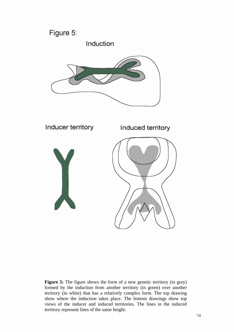
74

Figure 5: The figure shows the form of a new genetic territory (in grey) formed by the induction from another territory (in green) over another territory (in white) that has a relatively complex form. The top drawing show where the induction takes place. The bottom drawings show top views of the inducer and induced territories. The lines in the induced territory represent lines of the same height.

75

7 Tooth model

7.1 Introduction:

During last year we were searching an experimental system that uses MDMs. This was as difficult as expected, because there are very few systems in which there is a clear causal data explaining how pattern appears. In addition, for reasons we will later expose, the possibility of MDMs, although natural in a process like development, in which form is changing constantly, has almost never been considered. It is unlikely that researchers found this kind of mechanisms when they are searching other things. Hence, data from experimental studies is difficult to use because it has received some kind of interpretation by authors that were searching for other things. In spite of such big problems, we managed to found examples that are not for sure MDMs but that are quite likely MDMs. Tooth development is our best finding. It is a system for which many experimental information is available. Most of this information has been acquired very recently and, then, it is easy to found. Its development is very independent from the rest of the body. Its fossil (and alive) record is very well know, offering the opportunity to compare models with phylogenetic variation. For this system there was a hypothetical considerable consistent mechanism of formation (Jernvall, 2000), applicable to triconodont teeth (essentially two dimensional teeth). It is not very frequent that developmental biologists propose mechanisms for pattern and form and it is even more unlikely that they are proposed in a way that can logically function. This was not show in this case, but it was clear that it was something that could work by itself. We were able to modify such model into a mophodynamic one that was able to reproduce the three-dimensional morphology and patterns of gene expression of mouse (mus musculus) and vole (microtus rossameridionalis) second molars, among others that we are still studying. This is a very important result since there is absolutely no other model able to reproduce a complex three dimensional morphology from an implementation of the basic gene product interactions and cellular developmental functions (in this case, only mitosis really). In addition, there is not other model able to reproduce the form of so many species at the same time. This is specially relevant in relationship to how we understand that the causality in development has to be shown (see section 1.3). In other words, by reproducing as many as possible teeth types, we show how consistent is the model. In fact, the implementation of the model in contrast to the use of mere verbal arguments has allowed us to show that the model can actually work and study the variational properties of the proposed mechanisms. There are many problems in the evolution of development and evolution that can be approached by this model. I will only present those that we have already approached. For looking at the programs used in the simulations see annex IV.

76

8 Evolutionarily interesting characteristics of MSMs and MDMs 8.1 Methods: As we have seen, the tooth model is a MDM. There is a way to make teeth using a MSM. We have used a MDM mechanism because, from what we know about tooth development, a MDM is much more likely. Epithelium folding takes place while knots are sending signaling molecules and is actually affected by them. Which cells receive signals and with which intensity depends on how form is changing. At the same time how form is changing depends on the signals that cells are receiving. With the tooth MSM we have not been able to produce a mouse or a vole tooth. The tooth MSM works in the following way. It is like the tooth MDM but in this case neither activator nor inhibitor affect the growth of the epithelium or the growth of the mesenchyme. There are two phases: in one there is only signaling and lateral growth. The tooth is, thus, plane and diffusion takes place over a two-dimensional flat lattice. The lattice grows by apposition of cells in the borders according to a bias (multiplied by Rm) that is independent of activator or inhibitor concentration. Strictly, it is also a MDM, but only a small part of it has any kind of reciprocal affectation between form and signaling. At the end of this phase, a pattern formed by flat spaced knots has appeared. In a second phase the epithelium folds. Each row of cells in the epithelium attains a depth equal to a constant value minus the concentration of activator in this cell multiplied by Re. Thus, at the end, a multipeaked surface resembling a tooth appears ( See fig.6). There is also a way to produce teeth by a strictly MSM, however, it has not too much sense to try to simulate it. The mechanism is like the positional orthodox mechanisms presented in 6.1. Hence, the only thing that is needed is two gradients and a very precise mechanisms to interpret small differences of concentration. Then, each cell will take a depth determined by its singular result of interpreting the gradient. The problem is that such way to differentiate thresholds can be very complicated. Independently of how this mechanism is, it will need many genes and, in fact, what can be produced by the model is easy to see without requiring a model. .

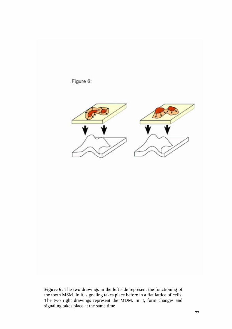
77

Figure 6: The two drawings in the left side represent the functioning of the tooth MSM. In it, signaling takes place before in a flat lattice of cells. The two right drawings represent the MDM. In it, form changes and signaling takes place at the same time

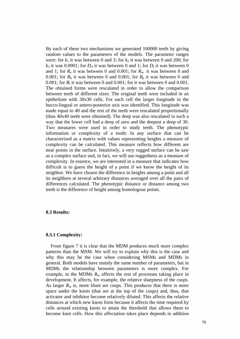
78

By each of these two mechanisms we generated 100000 teeth by giving random values to the parameters of the models. The parameter ranges were: for k1 it was between 0 and 3; for k2 it was between 0 and 200; for k3 it was 0.0001; for DA it was between 0 and 1; for DI it was between 0 and 1; for Re it was between 0 and 0.001; for Rm it was between 0 and 0.001; for Ba it was between 0 and 0.001; for Bp it was between 0 and 0.001; for Bl it was between 0 and 0.001; for it was between 0 and 0.001. The obtained forms were rescalated in order to allow the comparison between teeth of different sizes. The original teeth were included in an epithelium with 30x30 cells. For each cell the larger longitude in the bucco-lingual or antero-posterior axis was identified. This longitude was made equal to 40 and the rest of the teeth were rescalated proportionally (thus 40x40 teeth were obtained). The deep was also rescalated in such a way that the lower cell had a deep of zero and the deepest a deep of 30. Two measures were used in order to study teeth. The phenotypic information or complexity of a tooth: In any surface that can be characterized as a matrix with values representing heights a measure of complexity can be calculated. This measure reflects how different are near points in the surface. Intuitively, a very rugged surface can be saw as a complex surface and, in fact, we will use ruggedness as a measure of complexity. In essence, we are interested in a measure that indicates how difficult is to guess the height of a point if we know the height of its neighbor. We have chosen the difference in heights among a point and all its neighbors at several arbitrary distances averaged over all the pairs of differences calculated. The phenotypic distance or distance among two teeth is the difference of height among homologous points. 8.3 Results: 8.3.1 Complexity: From figure 7 it is clear that the MDM produces much more complex patterns than the MSM. We will try to explain why this is the case and why this may be the case when considering MSMs and MDMs in general. Both models have mainly the same number of parameters, but in MDMs the relationship between parameters is more complex. For example, in the MDMs Rm affects the rest of processes taking place in development. It affects, for example, the relative sharpness of the cusps. As larger Rm is, more blunt are cusps. This produces that there is more space under the knots (that are at the top of the cusps) and, thus, that activator and inhibitor become relatively diluted. This affects the relative distances at which new knots form because it affects the time required by cells around existing knots to attain the threshold that allows them to become knot cells. How this affectation takes place depends in addition

79

on already existing knots. Thus, the relative positions of existing knots affect the localizations where the new knots can appear. The relative sharpness of their cusps also affects where new cusps will form. In addition, the relative shapes of cusps and parts of the tooth affect how a concrete concentration of inhibitor will affect mesenchymal growth and in which direction. This, in turn, affects the relative dilution and concentration of activator and inhibitor. .

Figure 7: The figure shows the frequency of teeth with specific complexities. Dashed lines represent these frequencies for the 100000 made by a MSM and the straight line frequencies for the teeth made by MDMs

80

The growth of the epithelium has similar effects since it affect also the relative sharpness of cusps and, thus, the relative concentration of inhibitor and activator. At the same time activator affects epithelial growth. Kinetic parameters affect also growth since they affect how quickly activator and inhibitor will accumulate or in which relative proportions. In general, the whole dynamic can be seen by looking at form as a patterning force by itself. Activator and inhibitor concentrations affect each other distribution, but also the distribution of mitotic rates. At the same time, the changes in form attained affect, by relative dilution, the distribution of activator and inhibitor. This, in turn, affects form again. The intermediate phenotype can thus be said to constitute some kind of information that is used to reinterpret the genotype. In the tooth MSM the dynamic is much more simple. Rm can affect the formation of knots but it only determines whether there would be more or less knots, the exact localization of them being mainly equal for diverse values of Rm. Re does not affect at all where knots will form. Growth biases affect where knots will form but in a more predictable way since they determine where new cells will be added to the system and, thus, where new knots will form. But where this new cells appear is not affected by where knots form. Kinetics parameters affect the relative size and spacing between knots and also the deepness and sharpness of cusps. In essence, this model is just a reaction-diffusion model with growing, as many others (Varea et al., 1997; Kondo and Asai; 1995; Maini et al., 1991). To understand why the forms obtained by MDMs are more complex becomes more easy if we think on form as a causal factor in tooth development. At the beginning of tooth, development form is simple, with only one cusp. More complex forms appear later, when there is enough lateral growth. Depending on the relative sharpness of cusps, later cusps will appear in different places and with different forms. Actually, as more complex is an intermediate stage, more likely later stages will also be more complex. This is because form itself affects the dynamics of development at later stages. This does not happen in the MSM. In other words, the capacity of MDMs to use phenotypic information as cues or affectations for later development, produces that the MDM generates more complex forms for the same genetic information. We say the same genetic information because tooth MDM and MSM have the same number of genes, the same interactions between genes and the same cellular developmental functions. They only differ in how are they organized.

81

On the other hand, it is clear that the orthodox MSM can generate the more complex teeth possible for any number of cells. In fact, by this mechanism all the forms describable by a matrix of heights are possible. As each cell can take a different height value and all values are possible in a cell, all patterns are possible and then the more complex forms are attainable this way. In the MDM instead, the form dependency makes many patterns unreachable. The first form to form always consist in a cusp and this conditions all later development. The intrinsic interdependence between form and activator and inhibitor kinetics allows to generate complex forms more easily but does not allow to make many forms that are possible by this orthodox MSM (see section 9.1). This impossibility can be said to be a developmental constraints (in sense Alberch (Alberch, 1982)). 8.3.2 Morphospace: As we will see, some characteristics of the morphospace have very important evolutionary consequences. The morphospace reacheable by a mechanism is the whole set of patterns that can be produced by such mechanism from different prepatterns, w values and environmental conditions, ordered in a hyperdimensional space. In our case, the teeth produced by the model stay in a space of 1600 dimensions in which each dimension stands for the depth of a cell. Thus, each different tooth occupies a unique point in this space. In this section we present a set of useful measures calculated over this space in order to grasp some of their interesting characteristics. Of course, a direct visualization of this space is not possible. We will call MSM morphospace to the morphospace reacheable by the tooth MSM and MDM morphospace to that reacheable by the tooth MDM. The first measure we performed was a direct measure of the volume of each morphospace. This space turned out to be too large for our 100000 teeth sample. For this reason we decided to rescalate our morphospace and took a more coarse grained view to our teeth. Hence, we rescalated all height values to take discrete values between 0 and 128. The teeth were transformed from a matrix of 40x40 to a matrix of 10x10. Although many information is lost with this transformation all teeth looked roughly equal. The volume was calculated as the number of different teeth after this transformation. As all teeth turned to be different by each mechanisms we decided to calculate the volume for different degrees of coarse grained view. Thus, the volume occupied was calculated by rescalating height values between 0-128, 0-64, 0-32, 0-16, 0-8, 0-4, 0-2. So, in each case, the entire morphospace was partitioned in 128, 64, 32, 16, 8, 4 and 2 hyperboxes. The morphospace can be seen as a hyperdimensional box and by this rescalation we are partitioning it in hyperboxes of different size. The results are shown in figure (fig.8). It is clear, from these results, that the MDM occupies more morphospace, at least at a coarse grained view of the morphospace. For sure it only means that MDM teeth are more spread over morphospace. This means, at the same time, that MDM teeth are on average more different among them.

82

This measure does not allow many resolution in distinguishing the properties of the MDM and MSM morphospace. For this reason, we measured the distances between each tooth in each of the morphospaces and their five nearest points (that is, its five more similar teeth in the sample). The frequencies of the distances found are plotted in figure 9 (fig 9). It is clear from these figures that the teeth produced by the MDM use to be more different. When calculating the number of teeth that are at a distance smaller than 1000 for each teeth (fig.10 and fig.11) we also found that MDM teeth are more different between them. Why this is the case can be understand by taking into account the following reasoning: In the tooth MSM the growth parameters do not produce variation of the relative position among knots. Instead, the variation of these parameters can only produce that the cusps are more wide or more sharp. Hence, very similar teeth differing in the sharpness of cusps can be produced. Kinetic parameters can affect the relative height and spacing of cusps but they do it in a more or less gradual way. In general, as less interdependence exist between parameters of the model the effects of variating a parameter are small and do not depend on the other parameters through form, as is the case in MDM. This produces that teeth produced by the MSM are more similar.

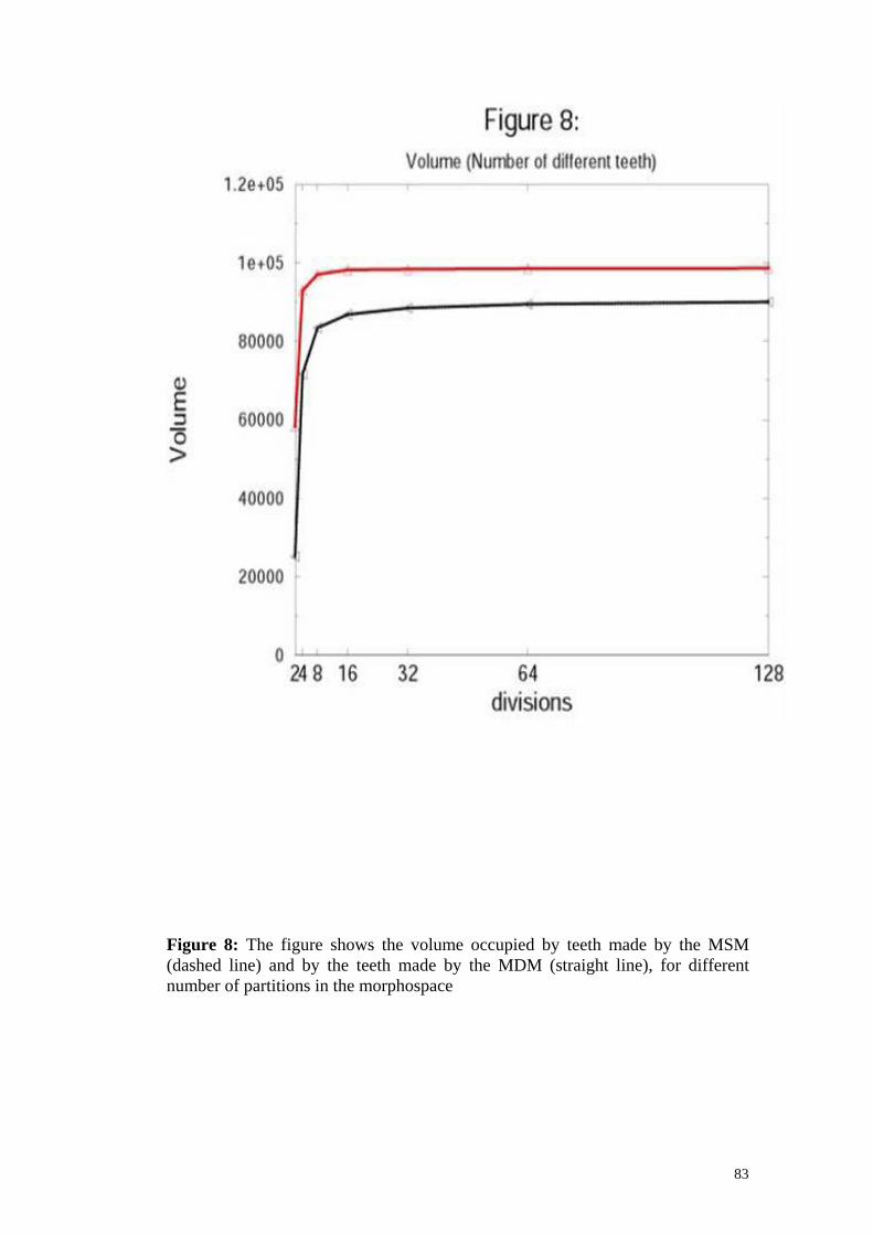
83

Figure 8: The figure shows the volume occupied by teeth made by the MSM (dashed line) and by the teeth made by the MDM (straight line), for different number of partitions in the morphospace

84

Figure 9: The figure shows the frequencies of the distances among the first, second, third and fourth neighbors of each teeth averaged for all the teeth produced by MSM (in grey) and MDM (in white).

85

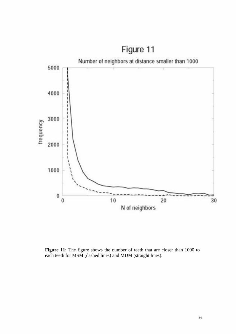
86

Figure 11: The figure shows the number of teeth that are closer than 1000 to each teeth for MSM (dashed lines) and MDM (straight lines).

87

In contrast, in the MDM any parameter change can affect, locally or globally, form and this can have effects over how the rest of the parameters affect development. In other words, as form change can affect the spatial distribution of activator and inhibitor and the distribution of activator and inhibitor can affect form, most changes in parameters are amplified to some extend producing that similar forms are not likely produced by similar parameters. This, however, does not preclude that similar forms can exist (they may be reachable independently of how similar are the parameters that give rise to them). The MDM has constraints in the variation they can produce. It is difficult to perceive but the intense interdependence among parameters in MDM precludes the existence of some intermediate patterns. Morevoer, we have found that different combinations of parameters can give the same patterns. This implies that the MDM morphospace is rugged with the intermediate patterns between two patterns not existing always. Morphospace ruggedness can be measured directly. As previously,the morphospace has to be partitioned in hyperboxes of different sizes. For each scale the number of occupied boxes (the volume) is measured. The number of non-occupied boxes in contact with an occupied box is also measured (that is the surface of the occupied volume). The ratio between these two measures is the ruggedness of a morphospace. As seen in figure (fig 12) the MDM morphospace is, as suggested, more rugged. The problem is that for most scales both morphospaces are maximally rugged (that is all occupied boxes are surrounded by unoccupied boxes) and, thus, it is clear that the sample is slightly small. 8.3.3 Genotype phenotype relationship:

We performed another set of simulations in which, as previously, random values were given to the parameters. For each tooth (we call this the wild type tooth) found we made 100 mutants (10 for each parameter) differing only in small random values (in the ranges for k1 it was ±0.0006; for k2 it was ±0,04; for k3 it was 0; for DA it was ±0.0002; for DI it was ±0.0002; for Re it was ±0.0000002; for Rm it was ±0.0000002; for Ba it was ±0.0000002; for Bp it was ±0.0000002; for Bl it was ±0.0000002; for Bb it was ±0.0000002). For each set the distance between the mutant teeth an the wild type tooth was measured. The frequencies of such distances for all the teeth analyses is plotted in figure (fig.13). MDM teeth clearly exhibit a more complex relationship between genotype and phenotype. The reasons for this have been explained in the last section.

88

Figure 12: The figure shows the ruggedness of the sample made of the morphospace of by the MSM (dashed line) and MDM (straight lines). The x-axis shows the number of partitions made in the potential morphospace.

89

Figure 13: The figure shows the frequency of distances among the teeth produced by similar sets of parameters in the MSM (dashed lines) and MDM (straight lines) morphospace.

90

9. Discussion 9.1 Properties for other MDM: The results just described hold for the model we have presented and probably for teeth. Our bet is that it also holds for MDMs in general. It has to be taken into account that the distinction between MDMs and MSMs is a quite generic one and that each DM may have its own evolutionary interesting properties. This MSM-MDM distinction is useful because the DMs in each category may tend to have the same evolutionarily interesting properties. In the following section we will try to show why we expect that the properties we signaled for the tooth MDM hold for the rest of possible MDMs and why the properties of tooth MSM also hold for MSMs in general. 9.1.1 Morphological disparity: For the same amount of genetic variation MDMs can produce more phenotypic variation. Moreover, the genetic information (number of genes and connections between them) required for a MDM to generate a certain amount of variation is, normally, considerably smaller than that required for a MSM to produce the same amount of variation. As we said, the spectra of territory forms that MDMs allow is considerably large because it includes all the forms that can be generated by intersecting all the territory forms possible by the DMs of form and state in different distances and relative orientations. w changes in the DMs of form can easily produce changes of form that can easily affect the relative distance between an inducer territory and an induced territory, the relative orientations and the form of any of them. The repertory of possible form changes in a DM of form is limited, but the effect that it would have over later patterning is only limited by the forms of inducer and induced territories. Let us suppose a MSM and a MDM that use the same basic DMs. In general, the range of genetic territory forms possible would be large for MDMs. This is because the changes in form produced by w mutations would have effects over the form of more territories. In addition, these effects would depend on the form of the existing phenotypes and would allow forms appearing from intersection between already existing forms in diverse angles and distances that are not possible by DMs of form or state alone. Hence, combining DMs in a morhodynamic way can produce more types of patterns. As it happens by combining the same DMs it is clear that this additional pattern variation that MDMs allow is attained from the same DMs and thus from the same genes and genetic information. Hence, MDMs can produce more morphological variants for the same amount of genetic variation. In fig.14 we present a hypothetical example showing this. We will later discuss real examples but, of course, it is difficult to found experimental examples in which a MDM and a MSM are using the same DMs (note that MDM and MSM are defined from how they combined form and state DMs), just because there are few

91

examples in which the formation of a pattern is understood. As we said, they are mainly those that only use DMs of state. MDMs not only can produce more pattern variation but they do it frequently. This is because w mutations can easily affect DMs of form, producing a form change that, although may be small, has consequences on how signaling takes place later. As basic DMs are more interdependent, in MDM w changes use to have more wide effects. In addition, MDMs make the patterning of a part of the embryo more affectable by the rest of the patterns of the embryo, specially if the rest of the patterns are also complex. w mutations in the rest of the embryo can produce a form change by which a territory that was supposed to induce a near territory, by sending a signaling molecule, is displaced an located next to another territory that also expresses the adequate receptor. In this case, development may proceed in a very different way. This kind of changes may require very small w mutations but can have quite dramatic effects that although are likely to be often deleterious may be implied in the origin of innovation when leading to neutral changes. w changes in the state submechanisms also can have different effect in MDMs and MSMs. In MSMs, signaling takes place at the beginning and, thus, the form produced depends on the territory forms of the initial conditions and also on the mechanisms of state itself. w changes like increases in the diffusivity of a signaling molecule would have effects, but these would be the same for the same initial conditions. In a MDM instead, the effects of such kind of changes would be different if a change in w in the DMs of forms has also appeared (see fig.14). In summary the ability of MDMs to use intermediate phenotypes as patterning information allows them to generate more variation.

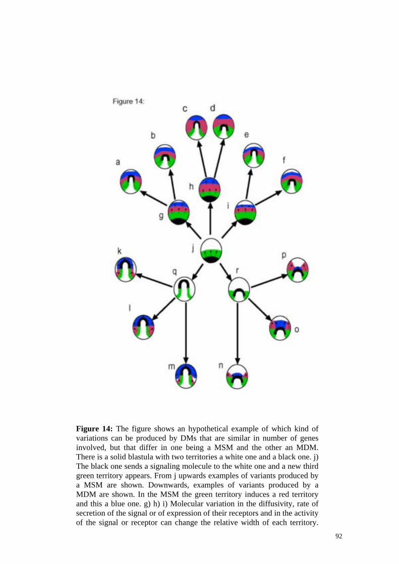
92

Figure 14: The figure shows an hypothetical example of which kind of variations can be produced by DMs that are similar in number of genes involved, but that differ in one being a MSM and the other an MDM. There is a solid blastula with two territories a white one and a black one. j) The black one sends a signaling molecule to the white one and a new third green territory appears. From j upwards examples of variants produced by a MSM are shown. Downwards, examples of variants produced by a MDM are shown. In the MSM the green territory induces a red territory and this a blue one. g) h) i) Molecular variation in the diffusivity, rate of secretion of the signal or of expression of their receptors and in the activity of the signal or receptor can change the relative width of each territory.

93

Later, the black territory invaginates. a) b) c) d) e) f) w variation in the DM that produces the invagination gives variable depth inside the blastula and takes variable amounts of green territory. In the MDM, before additional signaling takes place, the black territory invaginates. q) w variation in the form DMs can produce that this invagination goes deep inside the blastula taking thus the green territory inside the blastula or leaving it r) outside. Later, the green territory induces a red territory and the black territory the blue territory. k) l) m) n) o) p) w variation in the state DM can variate the amount of territory induced. In contrast, in the MDM case these changes do not only produce a change in the width of the new territory generated but can also produce a dramatic change in its form. In the MSM territory forms are mainly those possible by form and state mechanisms. These include for the state DMs wave like bands. In contrast, the MSM allows variation in territory forms that are is not simple waves and that are not easily producible by form DMs, state DMs or simple combinations of both.

94

9.1.2 Complexity: MDMs are also able to produce more complex patterns. It can be easily explained and generalized if it is taken into account that as the forms that DMs of form can produce can be used to induce neighbor territories the complexity of a pattern at any intermediate stage can be used to increase, through further inductions, the complexity of the pattern. In other words, MDM is the mechanism by which more complexity can be produced for the same amount of genes, because the intermediate phenotypic results that appear from the use of concrete DMs is used as an spatial "input" for subsequent DMs. 9.1.3 Relationship between phenotype and genotype : As we already said, the dependency of DMs of form on the material properties and form of potentially the rest of the embryo makes them to exhibit a complex relationship between genotype and phenotype. In MDMs, as the outcome of later acting state DMs depends on the form changes made by the DMs of form, this complex relationship between genotype and phenotype is also found. Hence, the interdependency between form and state DMs makes the relationship between phenotype and genotype much more complex than in the case of MSMs. In addition, the dependency on forms and relative orientations intrinsic to MDMs makes that sharp morphological transitions can happen for small w values (see next section). Inevitably, as MDMs allow to make more and more complex patterns for the same amount of genetic information, the correspondence between genetic and phenotypic information has to be more indirect. 9.1.4 Form of the morphospace: In the tooth model we found that the tooth MDM produce teeth that are more different among them. In general, we expect this to be the case for MDMs in general. It does not imply that MDMs can produce more patterns. In fact, we expect that in many cases MSMs can produce more different patterns although they will be more similar among them and, thus, would be more densely packed in the morphospace. The reasons for this are slightly complex and require some explanation. In general, most form mechanisms are inherently non linear (Beloussov 1998; Oster and Alberch, 1981) and, thus, some w mutations may have dramatic changes while others would not produce any change. When looking at the morphospaces produced by DMs of form they are spotty without intermediate forms among many forms but when the morphospace is compared with the parameter space it becomes clear that this non-linearity produces not only a complex relationship between phenotype an genotyp, but also that the same forms can be attained by different combinations of parameters (that can be similar or not). This produced that MDMs exhibit more strongly these characteristics in comparison to MSMs. But the dependency on intermediate phenotypes produces by itself

95

similar but more accentuated properties. The dependency on form produces some complex threshold effects that are difficult to evaluate (see fig.15). Hence, for example, the intersection between the inductor and the induced territory produces new territories that may exhibit sudden changes due to small w mutations or not change at all. For example, a change in the distance among an inductor and induced territory produced by a w mutation may have a dramatic effect like in figure 16a, a small effect like in figure 16b or no effect as in figure 16e. In addition, these effects may not have intermediates. The dependency on form allows to generate more different and more complex variation but at the same time forbids some intermediate forms. This is produced by the complex threshold effects that are exemplified in

96

Figure 15: The figure shows three territories. The grey territory secretes a signal that can induce a darker grey territory in the underlying flat white territory. w changes in the mechanism of form that produces the form of the grey territory and their orientation in relation to the white territory can produce changes in the form of the induced dark grey territories.

97

figure 16. Thus, there is a quite subtle relationship between development variation and developmental constrains. In addition, the dependency on form produce that, as we observed in the teeth model, the same or very similar patterns can be attained from similar or even very different w values or environmental conditions. For similar w values this is due to the non-linearity of form DMs and to these threshold effects of form dependency. When the same pattern can be found for quite different values of w it is because they have compensating morphological effects over form. For example, the same or very similar effects can be attained in some cases by decreasing the distance between an inducer and an induced territory, increasing the amount of signaling molecule secreted (or their activity) by the inducer territory, increasing the amount of receptor expressed (or they activity) in the induced territory, increasing the diffusivity of the signal or of the environment between inducer and induced. For more complex situations and phenotypes, this multiplicity of ways to attain a pattern is likely to be more acute. In addition, many of these changes can be produced by mutations in different genes. All this, in fact, gives some homeostasis to MDMs in spite of the variation they are able to produce.

98

In figure 17 (fig 17) we have plotted a pedagogic graphic of how would be a morphospace of a MSM and a MDM. MSM morphospaces are more spatially restricted but occupy space more densely. That is, with more intermediate patterns possible. The occupied morphospace is thus, a compact hyperdimensional bowl with a more or less regular form. In MSMs instead, the morphospace has a complex irregular form that is expanded over a larger part of the morphospace. Many intermediate patterns do not exist and for each pattern the existing neighbors may be in any direction thus giving to the morphospace a complex form. When comparing morphospace with parameter space or genospace more differences among MSMs and MDMs appear. In MSM this relationship is more direct with a more direct correspondence between a point in genospace and a point in morphospace. This relationship is more biyective with each point in genospace giving a different point in morphospace and with near points in genospace giving rise to near points in the morphospace. In MDMs in contrast, the same point in morphospace can be produced by different and even distant points in the genospace. In addition, near points in genospace can give rise to very distantly related points in morphospace. It is also the case that the nearest points to a concrete pattern in morphospace do not need to come from points in genospace that are also the nearest points to the genospace point that generates this point in morphospace. Hence, the occupied morphospaces and genospaces are not topologically equivalent in the case of MDMs. This description is only orientative. Concrete MSMs may have a morphospace form more similar to that of MDM if they use extensively emergent and form DMs.

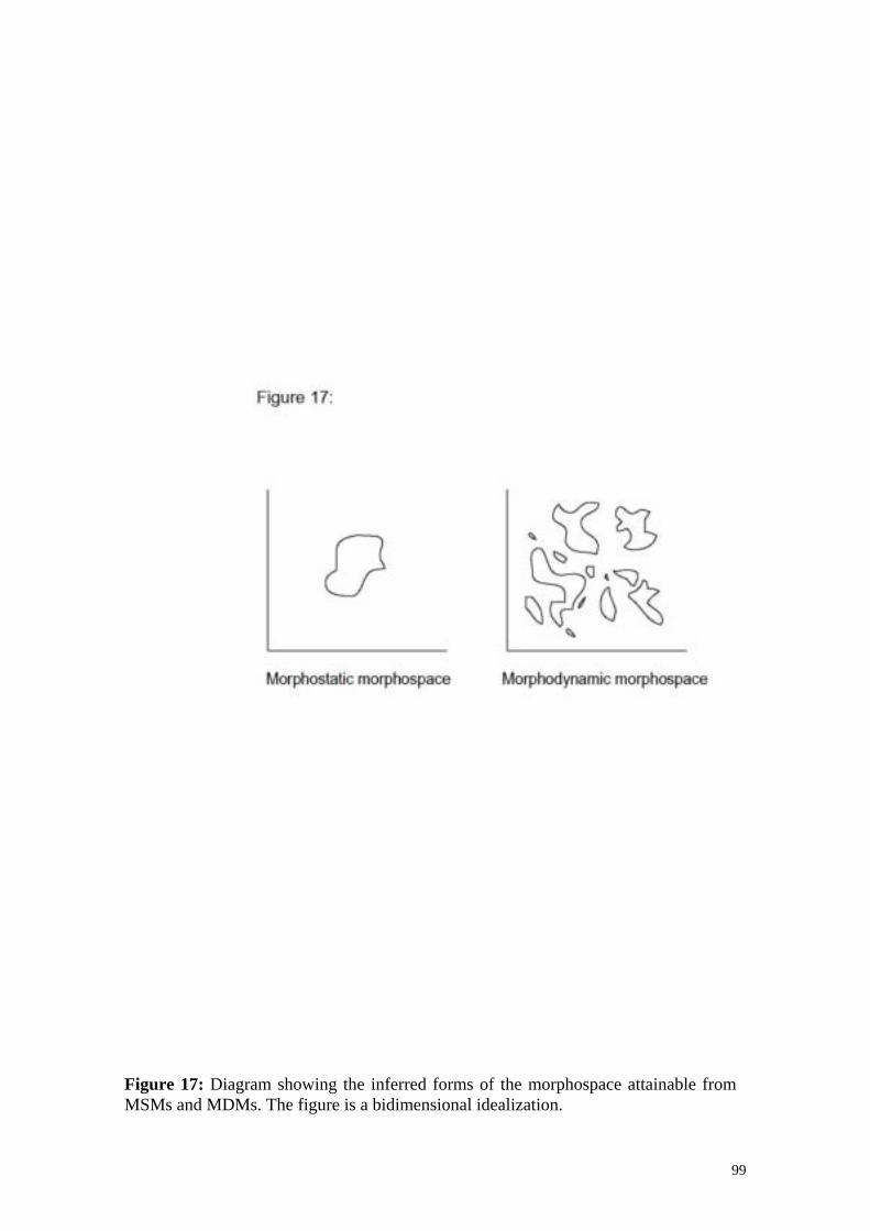
99

Figure 17: Diagram showing the inferred forms of the morphospace attainable from MSMs and MDMs. The figure is a bidimensional idealization.

100

9.1.5 Homeostasis: In general, MDMs seems to be less homeostatic to changes but it is something relative that may depend on the exact DM. In fact, the homeostasis of MDMs per se depends on the exact change. As we said, some small w mutation may not have any effect. This is not so likely in MSMs where most w changes will have and effect, although it would be often very small. On the other hand, as MDMs normally need to employ less genes for generating the same patterns the chance that a mutation disrupts the DMs by disrupting a simple gene is smaller. 9.2 Predictions: In this section, we will try to explain how all these results can be used to shed some light about evolution and development. In the next section we will discuss to which extent the predictions we present here fit existing data. 9.2.1 Dynamics of appearance and substitution among DMs: In general, we expect MDMs to be the type of DM involved in the generation of morphological innovation the first time it appears. Lets us concretize the problem. We can suppose that there is a population and that in some individuals some part of their bodies, that was in their parents spatially homogeneous, is spatially heterogeneous. We will call this newly heterogeneous part of the body a new morphological structure, and we will say that it is a morphological innovation. This is expectable in the cases in which the DM has been generated de novo but also in the cases in which an already existing DM has been simply recruited in a new developmental context or generated from mutation in an already existing DM. The reason for this is that MDMs can generate more morphological variation (and more complex) for fewer genetic information. By fewer genetic information we mean the number of genes and connections between them. Hence, the reasons are twice. MDMs can appear easily and, in proportion, produce many morphological variation but also MDM can produce many morphological variation by simple small w mutations. This is specially true for innovations that consist in relatively complex patterns. There is another way to argue why this is the case. In essence, it is the same case but explained in a more

101

concrete context. Let us suppose a morphological innovation that consist in the invagination of a part of an epithelia inside the embryo. It can be the case that after such movement this epithelia becomes localized near to territories that are sending molecular signals. The relative arrangement of such territories in respect to the newly invaginated territory will produce that groups of cells in the invagination receive a specific concentrations of signaling molecules. These cells would be arranged in concrete forms that depend on the relative positions between the invaginated epithelia and neighbor territories. It is very easy to use this already existing patterns to generate new form territories in the newly appeared invagination. The only molecular change required would be to make the invaginated epithelia to express a receptor for some of the signals received. This is a simple change if it is taken into account that the forms that can be obtained can be considerably complex. In essence, we expect MDMs to appear more likely, because for a large number of patterns the easiest way to generate them from molecular mutation implies to use a MDM. Two kind of argumentations can be used here. If we assume that what is going on is that in a certain environment there is a number of phenotypes that are more adaptive, we can argue that it is more likely that they are generated by a MDM because MDMs generate a larger number of patterns (or patterns more scattered over morphospace) for the same amount of genetic variation. If, contrarily, we expect that some environments are not very strict (because in many cases organism will be able to find (actively or passively) their better environment) then MDMs would still be the more likely option because as it generates more variation it is more likely that after some time most variants have been generated by MDMs. How complex a pattern has to be for being likely to be generated by MDMs is difficult to say and depends on the concrete system. We have not performed the selection simulations we performed for emergent and hierarchic mechanisms. For simple patterns ( for example for genetic territory forms resembling waves) MSMs may also be involved in innovation. However, even if a pattern has appeared through a MSM it is likely that it is substituted by a MDM one if their complexity increases (although as we will see it also depends on other facts). The combination of several existing MSMs can also produce complex patterns but in comparison to MDM they can not produce many other patterns through w mutations. Thus MDM is still the more likely mechanisms to generate complex patterns. Lets us consider this in more detail by considering which types of innovations and environments are possible. A possibility that is supposed to be common is that the innovation is initially neutral or nearly neutral. Contrarily to common wisdom, populations exhibit considerable morphological variation in some structures. This variation can be discrete and not gradual, and include whole morphological structure. In fact, if the structure is new and does not

102

interfere with the function of any other structure it is likely that it is not selected. This morphological structure would be free to vary (unless it generates maladapted variants) until it reaches an adaptive form. This scenario has been suggested to be usual in the origin of morphological innovations since Darwin (Walker-Larsen and Harder, 2001; Muller and Wagner, 1991; Darwin, 1859). In this case, the type of DM that more often would be implied in the origin of innovation would be a MDM. In many cases, however, MDMs would be substituted by MSMs that produces the same pattern. This would normally require many time, and would even be effectively impossible for very complex patterns. In any case, there are selective pressures, expectable in many environments, that would favor this substitution. First, MSMs offer a more close relationship between phenotype and genotype and allow more fine and gradual variation to be produced. This normally produces a smaller mutational load, that is a larger proportion of the offspring would be equal or nearly similar to the parents. This is normally adaptive by itself. This is specially true if the pattern is more or less adaptive and is not useful to vary it too much. This situation of conservative selection has been argued to be very usual (Wright, 1977). In addition, in an environment in which selective pressures may change favoring different but similar patterns, MSMs will more easily and quickly produce the adequate variation. In many cases, MSMs also allow the possibility to independently vary the parts of a pattern. This may be adaptive in many cases. In summary, it can be said that MDMs are more often involved in innovation but that there is a trend (that is not found always, because it depends on the type of variation that would be more selective) to substitute it. It has to be noted that we are not suggesting that DMs are selected by themselves. Contrarily, what we are suggesting is that over time, and in some circumstances, the variation that would be more adaptive is more often generated by MSMs and, thus, it would probably increase its relative frequency in the population until substituting the original MDM. Other kinds of selective pressures can also favor MDMs. Hence, a pattern that is selected in a very coarse grained way and that changes often can be more usually generated by MDMs and not be substituted by MSMs. This can be the case if what is selected is some whole characteristic of the pattern and not the exact details of it. This has been suggested to be the case for many butterfly wing patterns (Nijhout, 1990). In some butterfly wings, part of the selective pressures depend on the perception of the wing pattern that the predator receives. This is some thing difficult to know for sure but it seems that the adaptive value of different wing patterns is not dependent on the details of the design but on some general coarse aspect of the pattern. In addition, which are the more adaptive wing patterns can change from environment to environment due to their different perceptional context or to different predators. It is clear that, in these cases, to have the capacity to finely change the details of the pattern does not seem to provide any special advantage. Contrarily, to be able to make quickly large phenotypic changes seems more adaptive. Actually, for these patterns, and for skin coating patterns in mammals, emergent mechanisms have been suggested. Emergent mechanisms have properties very similar

103

to those of MDMs and, in fact, we expect MDMs to be quite often involved in the patterns on which these kinds of selective pressures act. In contrast, in environments in which selective pressures over a pattern are very strong and fine grained a MSM is more expectable to be found in the formation of innovation. It holds specially, if the part of the body in which the innovation is, was under this kind of selective pressures even before the apparition of the innovation. In such cases in which only very small phenotypic changes are likely to improve the adaptive value of the pattern, MSMs are likely to be the DMs involved in the origin of the innovation. As far as this kind of selective pressures act, a MSM is not likely to be substituted. It implies that, in general with such kind of pressures, phenotypic complex patterns are much more difficult to appear. It is important to note, however, that MDMs can really generate complex patterns much more easily. This is so extreme that unless the selective pressures acting in a structure are very strong and gradual, MDMs would be the DMs that first generated an innovation. One of the principal problems of this approach is that, as we already noted in the introduction, there is not too much data about how are the selective pressures acting on phenotypes. Although the importance that it has, and the amount of literature devoted to defend more or less gradual selective pressures, there are really few studies that try to look this experimentally. There are many works showing that some populations are constantly changing by small changes. In these cases, the focus is on the changes at the molecular level (in many cases without clearly stating that the molecular variation does not need to be related to morphological variation) but there are also works looking at these changes at the morphological level in the fossil record. Unfortunately, in these cases the variation is looked as a product of selection but how is the variation before selection is almost never studied in spite of the considerable amount of data concerning artificially induced mutations. This is a quite important problem for the conclusions of these studies (specially when looking at the tempo and mode of evolution) since it is not possible to discern if evolution in this organisms is as it is because the nature of selection or because the nature of variation (or because some complex relationship between these two factors, as is probably the case). 9.2.2 The structure of development: The dynamics of origination and substitution just outlined can be used to explain some aspects of the structure of development. The predictions we will cast concern mainly the relative frequency of these two types of DMs in the different stages of development. It is in fact, a subtle task since which DMs are used in a lineage conditions its subsequent evolution and thus affect which new DMs will appear in the lineage. Hence, in general the structure of development would depend on the whole environmental history of a lineage. In other words, to fully understand it, an understanding of the trajectory over environments in time that a lineage has followed, is needed. It is, at its turn, tricky, since the environments reachable by a lineage also depend on the DMs it uses. Thus we need to

104

present it by describing different evolutive contexts and which would be the evolutive trends in them. It is expectable that, normally, developmental changes with consequences in the final phenotype (and not only in intermediate developmental stages) occurred more often at later developmental stages because there the changes do not need to be compatible with many other posterior DMs. In other words, later development is less entrenched than early one. In the cases in which innovation appears by MDMs but it is not the more adaptive way to produce the pattern (as we explained in the last section) we expect that MDMs would be substituted by MSMs over time. For very complex patterns this would take many time. This substitution may take place in some parts of the DM more easily and thus mixed DMs may exist during a time. In many cases two DMs, a MSM and a MDM, may coexist. In general, having two mechanisms producing the same can be adaptive since it buffers development from epigenetic errors and environmental fluctuations. This is because the range of situations in which the pattern would be formed is larger. In addition, mixed mechanisms have intermediate properties between MSMs and MDMs that may be adaptive in many contexts. Parts can vary independently to some extend but complex patterns can be attained. In addition, not so much variation can be produced because the MSM part can freeze the pattern to some of the variants that the MDM can produce. As this substitution, being it total or partial, requires some time we expect older mechanisms, acting relatively early in development, to be more frequently MSMs while later more new DMs would more often be MDMs. There are additional reasons for this. MDMs can produce many variation and complex variation but it can do it specially if the phenotype is already complex. In fact, when the phenotype is complex innovations by MDMs can appear very easily. In any organisms very early development takes place with few cells. The patterns present in morulas and blastulas use to be so simple that the more easy way to produce them is by MSMs (as we will see there are other reasons for this). In general, it is expectable that large changes in early development would more often disrupt development and thus, even if a pattern in early development was not originally generated by MSMs, it is expectable that it would finally be generated by a MSM. If the whole development itself is long with many stages, we expect that it can not be composed exclusively of MSMs. This is not only because complex patterns are difficult to attain or substitute by MSMs but also because complicated MSMs have some problems by themselves. If the pattern to attain is very complex and requires many stages, the number of genes required to form it through a MSM would be very large. In comparison a MDM would require many less genes. It produces that the

105

mutational cost of the MSM can become even stronger than that that MDM normally have. This is simply because MDMs use much less genes. This is more likely to happen when more complex are the patterns. 9.2.3 Phylogeny, disparity and environment: By knowing which type of DMs are more used in a lineage in general or in the formation of a pattern, some predictions about the mode and tempo of morphological evolution are possible for such lineage. It is specially possible if something about the environment in which such lineage is living is known and/or if the predictions are made for short time intervals in which the development is expected not to change too much. When looking at the evolution of a lineage that uses MSMs extensively, some patterns of variation in the phylogeny are expected. In comparison with lineages using MSMs more widely, it is expectable that lineages using MDMs extensively have larger morphological differences among the different branches of the lineage. Hence, when comparing species with similar times since last common ancestor, the lineages using MDMs may tend to be more different morphologically. This holds for relatively long time scales. For shorter time scales instead, MSMs would show larger morphological differences among species with similar amounts of time since last common ancestor. It is due to the more direct relationship between genotype and phenotype that MSMs allow. MSMs allow to quickly adapt to small environmental variations. Of course, it also depends on the kind of environments in which a lineage is living, but it is important to note that lineages will tend to sort into environments that are more adequate by their variational properties. In lineages using MDMs, morphological changes over very short time scales are unlikely because the kind of variation they normally produce is frequently relatively large. It is interesting to note that it is large in comparison with that produced by MSMs but that it does no imply that it is really large. Unfortunately, there is few data concerning how large is the variation produced by MDMs nor of how large has to be variation in nature for being too large. In general, it is expectable that most variation produced does not produce an increase in fitness and that relatively large variations are adaptive less often. Thus in lineages using MDMs variations that would be fixed in the population would appear less often, and thus, the populations would remain without changes (stasis) for most of the time. This is not so expectable if the environment has coarse grained selective pressures that change often. In these cases, relatively large variation would be found for short time scales. If the capacity of variation is large enough and the number of adaptive phenotypes comparatively small, variants would appear to be sorted randomly in a lineage. Note that in some cases (for example in teeth) the same patterns can be produced by very different w values, so DMs can produce some very different favored variants quickly. In these cases, this pattern would be of small taxonomic validity because closely related species can have very different patterns and relatively distantly related species can exhibit the same pattern. In MSMs lineages small variations are very easy and, thus, changes

106

over short time scales are more likely. In other words, MSMs lineages can respond to changes in selective pressures, not necessarily better, but at least more quickly. This variation is very gradual and actually true innovations are difficult. In fact, the evolution of such lineages would tend to be small for large time scales with some kind of recurrence or erratic evolution. Based on assumptions on the geologic record, some authors (Sheldon, 1996) have suggested that these two types of regimes may be identifiable. This is not based on the internal variational properties of organisms and is focused on geologic time scales that may be much more larger than those expectable here. Other authors have suggested that this kind of evolution would be expectable in r-strategists (Margalef, 1991) while others have suggested that the kind of evolution we suggest in MDM lineages would be very usual in vertebrates (Wake et al., 1983). In general, as MSMs produce more gradual variation when looking at phylogenies, more “intermediate” phenotypes between other existing phenotypes would be found. Hence, phylogenies would be more easy to reconstruct. If the amount of variation generable by the existing MSMs is small, however, recurrence would be frequent and thus phylogenetic reconstructions based on the phenotypes would be difficult too. In MDMs lineages, as no intermediate phenotype would exist, phylogenies based on morphology would be difficult to reconstruct. As we explained, MDMs would be more often involved in the origin of innovation even if the actual DM producing a structure is a MSM. This implies that when looking at the evolution of an innovation it is expectable that the fossil record of this is very scarce at the beginning, when this structure appeared. In addition, the phenotypic variation among early fossils is expectable to be larger than in later ones. In contrast, the fossil record of an structure is expectable to be more complete and with more gradual variations among fossils when the DM is substituted by a MSM. 9.3 Existing evidence: As we have already noted, there are very few developmental systems in which it is causally know how pattern formation takes place. Many of our predictions are about the relative frequencies of different types of DMs. Present data is insufficient to see whether these predictions are true or not. Here we will present some arguments that point that this kind of predictions are testable and would be tested in a near future. We think, however, that the identification of the possible types of DMs we have made is very useful for the field of evolution and development because it can aid to interpret and reinterpret many experimental data that is, in our view, underestimated or misinterpreted. To know what is possible and its evolutionary implications aids in designing experiments and formulating consistent hypothesis about how concrete DMs work. In the next section we present some examples of this. In a more broad scope, the predictions

107

made allow to recruit new tools to explain some general characteristics of development and evolution. 9.3.1 Experimental evidence for MDMs: In general, the experimental evidence for MDMs is scarce. As we will later discuss, this is probably due to some technical and sociological problems with MDMs. MSMs are more close to the expectations and assumptions of many developmental biologists but, just because it is more close to what is assumed, there are very few cases trying to show that a MSM works. There is a large amount of evidence about aspects of developmental processes strongly suggest that MDMs may be involved in development very frequently. Most developmental biologists would agree that form changes in development can occur simultaneously or intermixed between signaling events. By this argument it can be claimed that MDMs exist in development. The question can be how often or how important is that some DMs are MDMs for understanding its functioning and evolution. That is, the MDMs existing in nature are they strong MDMs or, instead, the morphodynamic nature of DMs does not need to be taken into account in order to efficiently understand development and evolution? In this section we briefly summarize some of the experimental data that seems to point to the involvement of MDMs in certain DMs. The evidence is incomplete. It is interesting to note that we review experiments that are not designed to show what we try to show and that in many cases it is likely that the published results are pre-interpreted in a biased way that may be difficult to filter (this is nothing special of such works but expectable in all scientific research). We restrict ourselves to only some cases. Different parts of vertebrate somites express different transcriptional factors due to the receiving of multiple signaling molecules from neighbor tissues. Notochord and ventral neural tube express the diffusible molecule sonic hedgehog (SHH) that is responsible of making the nearest somite cells to express transcriptional factors (at least pax1 and I-mf (Smith and Tuan, 1996; Chen et al., 1996)) required for becoming the sclerotome (tissue that will become the ventral connective tissue of the trunk (Johnson et al, 1994)). Wnt1 and Wnt3 are expressed in the dorsal neural tube and induce the nearest somite cells to express markers of epaxial musculature (Ikeya and Takada, 1998). Bone morphogenetic protein-4 secreted from the lateral plate mesoderm and Wnt secreted by the ectoderm make the more lateral part of the somite to express markers of lateral hipoaxial musculature (Dietrich et al., 1998; Pourquié et al., 1996). The relative arrangement of these territories in the somites depends on the relative arrangement of the inducing organs and alterations in this change somite patterning. The relative positions and forms of inducing tissues can change along the time while these inductions are taking place and is in fact a product of the relative growth of these organs. Thus, changes in form have a causal role in the genetic patterning of the somites. The patterns and forms implicated in this example are relatively simple.

108

In examples involving more complex structures , forms and morphogenetic mechanisms can be argued to have a more important causal role. The vertebrate brain is a complex morphological structure that initially forms from the folding of an epithelial tube. It has been proposed that the developing brain is subdivided into territories expressing specific adhesion molecules and transcriptional factors (Rubenstein et al., 1998). Specific signaling molecules expressed in the territory boundaries are supposed to pattern the brain. pax6 is a transcriptional factor that is known to affect the expression of adhesion molecules (Stoykova et al., 2000). In the mouse brain, during stages E9.0 to E12.5, pax6 is expressed in territory boundaries where the neuroepithelium is folding (Grindley et al., 1997). Pax6 mutants exhibit morphological abnormalities from these stages due to the partial failure of such folding. In such mutants the spatial patterns of expression of the genes expressed in the boundaries is altered (Grindley et al., 1997). This probably coincides with the changes in the shapes of the contours of the compartment that the lack of pax6 expression produces. In this case thus, the spatial pattern of expression of some genes is dependent on how the neuroepithelium folds. The cells expressing such genes are probably the same in the mutants and wild types. It is their change in spatial arrangement that produces later changes. At least, two of the genes affected are signaling molecules. Wnt7b is a diffusible protein that affects proliferation and adhesion (Brault et al. 2001), so it can affect compartment shape at the same time than pax6. The interesting thing is however, that the effect of pax6 over morphology depends on existing morphology. This depends on WNT7b too, and that the form of Wnt7b territory depends on pax6 effects over form. So the effects of both genes on morphology may depend on each other effects. Hence, changes in the patterns of expression of genes at the boundaries cannot be understood without understanding how changes in adhesion and proliferation rate affect form. Signaling molecules expressed in the boundaries are involved (Grindley et al., 1997) in the patterning of near cells, so in addition to all these effects, form and morphogenetic mechanisms have a causal role in determining patterning in later stages. This strongly suggest that brain uses strong MDMs. The inner ear is a vertebrate organ that can attain a considerable morphological complexity. Brigande (Brigande et al., 2000) proposed a hypothesis about how the early chick otic vesicle is patterned. They proposed that signals emitted from the rhombomer five produces the expression of specific transcriptional factors in the anterior half of the vesicle . Signals emitted from rhombomere six produce the activation of specific transcriptional factors in the posterior part of the vesicle. The otic vesicle is slightly ventrolateral to the rhombomeres. Thus, they propose that this signaling takes place when the vesicle is still not closed. At the same time, the still near ectoderm send signals that affect the rest of the vesicle. Later vesicle closes. The form of the vesicle when it is closing is important because it determines the form of genetic territories. Just prior to the invagination, pax2 is expressed in the anterior-posterior interval of the dorsal ectoderm that would form the otic vesicle (Hidalgo-Sanchez et al., 2000). pax2, as pax6, seems to be required for the invagination itself. Mutants like Kreisler and hoxa-1, that affect the form of the rhombomeres

109

affect also the form of the otic vesicles without being expressed there (Torres et al., 1998; Mark et al., 1993; Deol, 1966). These genes are known to be non expressed in the otic vesicle when malformation start. After closure, the otic vesicle is known to have at least two genetic territories. Each expresses different genes, principally transcriptional factors, growth factors, and adhesion proteins (Represa et al., 2000). Later, different areas of the otic epithlium start to exhibit different mitotic and apoptotic rates, producing the folding and invagination of different parts of the vesicle (Lang et al., 2000). These form changes are know to depend on the expression of concrete adhesion molecules (Legan and Richarson,1997). Hence, it seems that the spatial regulation of adhesion, mitosis, and apoptosis allows to produce the inner ear form. These form changes affect territories that are secreting signaling molecules. For example, BMP 4,5 and 7 (Oh et al., 1996), FGF3 and FGF10 (and their receptors) (Pirvola et al., 2001) are expressed in territories that change in form considerably during ear development. Some of these signaling molecules that are know to have dynamic patterns of expression affect mitotic rates (and thus form) (reviewed in Oestler and Hume, 1999). Hence the form of new territories depends on how the form of these signaling territories have changed and on how these affect the DMs of form in all territories. All this evidence let us to suggest that inner ear uses MDMs. Vertebrate craniofacial development is among the more complex processes in metazoa development. It involves spatiotemporal complex interactions between tissues originated from ectoderm, endoderm, mesoderm, neural tube and neural crest. Vertebrates exhibit a huge amount of morphological variation, as a group, in the forms of jaws and skulls. Many growth factors are simultaneously expressed in the developing branchial arches. These genes exhibit very dynamic patterns of expression. This is because they are expressed in areas that are constantly changing its form and because they affect each other expression by inhibiting the responses of other growth factors. The growth factors affect which transcriptional factors are expressed by cells and, directly or indirectly, adhesion and the mitotic and apoptotic rates of receiving territories (and thus their form). In chick early branchial arches FGF8 is expressed mainly in the contact area between ectoderm and endoderm, in the branchial pouches (Veitch et al., 1999). The form of the territories expressing such signaling molecules changes dramatically as face forms. Other FGFs and their receptors also exhibit dynamic patterns of expression around the branchial arches (Richman et al., 1997). BMP7 is expressed in wide areas of the branchial pouches. By bead experiments it has been shown that BMP7 induces the expression of msx1 and msx2, BMP4 and mitosis. (Yu-Hsuing, et al., 1999). In fact, the initial growth of the branchial arches seems to respond to concrete patterns of BMP7 expression in the pharyngeal endoderm and to form changes produced by adhesion changes mediated by pax1. By transplantation experiments, pax2 has been shown to mediate the invagination of some competent epithelium (Shamin et al., 1999). Pax1 is expressed just where ectoderm and endoderm fold to form the branchial pouches (Crossley et al., 1995). msx1 activates mitosis while

110

msx2, activates apoptosis in the cells where they are expressed (Veitch et al., 1999). BMP4 also activates msx1 and msx2 but in addition it activates fgf8 and shh (Barlow et al.,1997). Both BMP7 and 4 are strictly required for the growth and form changes that the branchial arches undergo during face development (Yu-Hsuing, et al., 1999; Barlow et al.,1997). They also affect cartilage formation (Semba et al., 2000; Shumm Barlow et al., 1993). BMP4 also activates Dlx2, as FGF8 do (Thomas et al. 2000). FGF8 also activates the transcriptional factor Lhx7 (that inhibits Gsc), Pitc1 and msx1 and the signaling molecules BMP4 and endothelin1. Moreover, FGF8 affects mitotic rate and apoptosis and is strictly required for branchial arch growth (Trumpp et al., 1999). FGF8 expression seems to be repressed by BMP4 (Shigetani et al., 2000). Some transcriptional factors like Barx1 are activated by FGF8 and inhibited by BMP4 (Barlow et al., 2000). The branchial arch form seems to appear by the action of multiple signaling molecules. Their territories of expression change in form during branchial arch development and thus the area receiving such signals also changes. The form of the territories of the genes downstream of these signals depends on the signal received but also in the form of the inductor territory and on how it changes over time. Hence, genetic patterning in the branchial arches can not be understood without understanding how form is changing. Signaling molecules affect, as we have seen, mitotic rates, apoptosis and adhesion and thus, form depends on the form of the signaling territories and the form of the signaling territories depends on how the signals emitted affect the form DMs. Hence DMs of form and state are strongly interdependent. In summary thus present evidence suggests that facial development uses MDMs. 9.3.2 Research problems with MDM: That the form of inductive territories change by DMs of form is something easy to accept. That DMs of form have the properties we point has been acknowledged by many authors. That this relationship between DMs of form and state can be causally very important in some DMs is not considered normally, nor at least as explicitly as here. In other words, it is acknowledged that DMs of form are important and that DMs of state are important but the causal dynamic effects that arise when both types of DMs act together is not taken into account. There are multiple potential reasons for this and it will be interesting to point some of them, since its presentation aids to understand the nature of MDMs. Early developmental biology was eminently observational, with a considerable effort in the description of morphology. Experimental embryology showed that some tissues are able to secrete some substances that change the fate of receiving tissues. A considerable effort was undertaken in order to identify the chemical nature of such substances. In most cases this nature has been already identified. Morphology itself is now seen as something without a causal role. But, when an induction takes place, there are two important aspects of the inductor and induced territories. One is the signaling molecules secreted by the inducer cells, or the receptors for them, existing in the receiving cells. As important as this is the form of the inducer or receiving territory. These two forms confer

111

spatial information that, in MDMs, can be as important as the signaling molecules for attaining the correct final patterns. To study a DM that is likely to be a MDM is difficult. First form and patterns of expression (that is the form of genetic territories) needs to be perceived with a considerable precision. Most studies take much more attention to which are the genes expressed than to with which form they are expressed. Patterns of gene expression are presented in one or few histological sections or in whole embryos at low magnification. In some few systems, however, three-dimensional fine reconstructions of morphology and gene expression are frequent. Of these, the more well known are inner vertebrate ear (Oh et al., 1996) and mammalian teeth (Jernvall et al., 2000). Some groups have recently started long-term projects for improving the capacity to reconstruct three dimensional morphology and gene expression (Streicher and Muller, 2001). We are convinced that such effort would facilitate the recognition of the importance of MDMs. The existence of MDMs, in fact, suggest that such approach is strictly necessary to understand many developmental systems. In addition, there are some views, like Wolpert's one, that accentuate this un-morphologic bias. The genetic program concept and the positional information concept give the mechanistic importance to what happens inside cells. One of the side-effects of this view is that, as cells are able to autonomously and precisely behave in order to make macroscopic patterns, it is not important to see if inducer tissues change in form. This is because cells "know" what to do. In fact, it is not even important to worry too much about how pattern formation takes place because what is important is how pattern is interpreted by cells. This reductionistic view a priori implies that form changes as a consequence of the genetic programs and, thus, it has not a causal role. This view does not give causal importance to form but to genes, and especially to transcriptional factors, as principal encoders of the genetic program. The existence of MDMs suggest a very different picture of development that is much more similar to that exposed in section 2.3. Cells are “stupid”, they have some sort of genetic program but it is very simple. It is more correctly described as an internal response table. Cells undergo simple responses to received signals. These consist in the activation of cellular developmental functions. The internal table is determined by the interactions between transcriptional factors and the transduction signal pathways activated by the signaling molecules receptors. Complex patterns emerge by the coordination through signaling and form changes of large number of stupid cells. Hence, patterns emerge from the collective behavior of groups of cells that can only communicate very simple, and molecular, messages and do very simple things locally (although their effects, especially in form DMs can be global). The work presented here shows that such coordination can easily be attained and that it can produce quite complex patterns like those of teeth. In addition, we show that it is not only possible but it is also the more easy way ( it requires less molecular variation to appear) to generate phenotypes of the complexity we observe in metazoa. To perceive how MDMs works has, in our opinion, some complexity. In addition, it suggest that research in developmental biology has to give,

112

relatively, less attention to genes (but of course, they are still fundamental) and give more room for research in morphology coupled with gene expression and non-genetic manipulations. This morphodynamic paradigm has the advantage that predictions are more falseable than in the case of positional information and genetic program paradigms. These later concepts are too flexible and can be used to accommodate a too large group of experimental evidence, as we have seen. Another reason that has made difficult the identification of MDMs is that it requires to understand, at the same time, DMs of state and form. They are normally studied in isolation. Moreover, for technical reasons, studies in development consider, normally, small temporal intervals. As we have said, DMs acting in short time intervals can not be MDMs nor MSMs. In addition, it has been more easy technically to study the same gene in different developmental systems than to study all the genes in a simple developmental system. This produces that there is many information in developmental biology but, with few exception, it can not logically and mechanistically be related because there is very few information per system. MDMs, due to the complex interdependence they exhibit, are difficult to understand by theory free manipulations of few gene functions. In contrast, MDMs require precise visualization of form and patterns of gene expression and the capacity to make and follow subtle developmental alterations. These alterations need to be made in the state submechanisms and in the form submechanisms. Subtle alterations in the state submechanisms are technically difficult but are feasible by current technology (transgenes whose expression can be temporally and quantitatively regulated can be made). If not, there are already many alleles that are w mutations of the wild type gene. Subtle alterations of form mechanisms are strange in the literature. These need to alter cellular developmental functions other than signaling directly or through genetic alterations that are know to affect only this. Another possibility is to alter form directly. Although it can be technically easy (not in complex phenotypes like the teeth for example) it is made only occasionally (Alberch and Gale, 1983). This was more usual in old days, when technical capacities were smaller. 9.3.3 Examples of substitution among DMs: As current causal knowledge about real DMs is scarce most of the predictions made here cannot be tested from existing data, but can be tested by acquiring new data and designing new experiments. Some estimations can be made if some of the predictions are taken as true, provisionally. For example, the different variational properties of MDMs and MSMs can be used to infer which DMs is using a lineage. This can be done by looking at the realized variation in a lineage and assigning to it the type of DM that produces similar variation. A system in which this may be potentially possible is the vertebrate limb. Early limb fossils (Coates and Clack, 1990) show a considerable

113

variation. The number of digits is very variable in these fossils while in the rest of tetrapods a maximum of six digits is found. The size, number of phalangeal bones and the number of carpal/tarsal bones is also more variable than in the rest of tetrapods. Reaction-diffusion mechanisms (Newmam and Frisch, 1979; Maini et al., 1991) and mechanico-chemical similar models (Oster et al., 1985) have been show to reproduce chondrification patterns, like those found in the limb under realistic assumptions. Later work (Miura and Shiota, 2000) has add some experimental data in support of the reaction-diffusion model. These models are unable to finely reproduce the anterio-posterior asymmetry exhibited by the pattern of chondrogenesis in the limbs. A considerable amount of data about signaling centers in the developing limb has accumulated in last decades (Gilbert, 2000). One of them, the AER (apical ectodermal ridge) secretes some FGFs that are know to activate mitotic rate in the underlying mesenchyme (Gilbert, 2000). Its signaling is also necessary for establishing the position and existence of the other signaling center of the limb; the ZPA (zone of polarizing activity). It also affects mitotic rate in the underlying mesenchyme. It is done, at least, by the secretation of BMPs by the cells receiving SHH from ZPA. These BMPs are known to inhibit mitosis (Ferrari et al, 1998). The effects on growing of both signaling centers produces that they become a part from each other. In fact, it is a MDM since the form of the signaling centers is affected by the growth of the underlying mesenchyme and the growth of the underlying mesenchyme is affected by signals. How the polarizing effect of the ZPA is produced is not known. An interesting possibility is that the original MDM have been partially substituted by a MSM that may have restricted the variation in limb to that actually observed, although this restriction may be skipped in many mutants. 9.3.4 Disparity and time since last common ancestor: The advent of molecular genetics has revolutionized the field of phylogenetics. For many groups there is a considerable amount of data concerning the times since last common ancestor among different species. This information is strictly necessary for studying many aspects of evolution. Potentially, the characteristics and rates of morphological evolution in such groups would be affordable or at least describable. As we do not know which mechanisms are used in each lineage we can not test our predictions about how the use of concrete DMs affects the rate and type of morphological evolution. In many cases, the historical and ecological factors that may affect this in a lineage are not known. There is some data that is, in spite of this, suggestive. Predictions are more easy to test if complex patterns are always produced by MDMs. Whether it is the case or not, is not know but comparisons can be made by using rough estimations of which kind of DM is more frequent in a group. For example, it is probable that MDMs

114

are more frequent in vertebrates than in nematodes. Nematodes have been taken as a group in which development, in comparison to other metazoa, makes an extensive use of autonomous mechanisms (Sternberg, 1991). Although this may not be as true as suspected (Schnabel, 1995), nematodes do not make many morphogenetic movements during development. They gastrulate (Knight and Wood, 1998), migrate some cells individually (Shemer et al., 2000) and change whole body form in late development through epithelial cell stretching (Chin-Sang and Chisholm, 2000). In comparison to vertebrates, nematodes have very few cells. Inductions use to take place from individual cells to individual cells, and normally inductions take place between cells that are not being moved. In this situation the DMs would not be morphodynamic very frequently. This let us to expect that, in general, vertebrates have species that are more different morphologically for the same time since last common ancestor. No quantitative estimation of the disparity among nematodes and among vertebrates has been made. However, it is suggestive that the time since last common ancestor between families of nematodes is larger than that existing among classes of vertebrates (Vanfleteren et al., 1994). 9.3.5 Variational properties of development and general characteristics of development: A group of authors has dedicated some effort to identify some general characteristics of development. Horder (Horder, 1989) suggested five general characteristics of development based on the study of limb development.

1. For a concrete morphological structure, the number of phenotypic anomalies that can be produced by different mutations is small. Hence, we have a limited number of variants. Each can be produced by different mutations.

2. When considering a morphological structure, like the limb, few parts of it can be varied independently.

3. Most mutations affect several aspects of the phenotype. They are thus pleiotropic.

4. The phenotype of a mutation vary from individual to individual 5. Many phenotypes produced by mutation can be phenocopied. The last decades of research in the molecular basis of development have revealed a number of features common to the development of all metazoa.

1. There is a limited number of signaling molecules and receptors for them. They are used many times during development and in very different contexts. The responses they produce depend on the previous state of the cell. These molecules fall into a small number of families of homology sequence. Members in a family may have partially overlapping downstream genes. These signaling molecules and their receptors are considerably conserved among metazoa.

2. Transcriptional factors and transduction pathways molecules are also considerably conserved among metazoa. The molecular function of these genes is considerably conserved. Most of these genes are

115

recruited in different moments in development. 3. Many development events, like fertilization or gastrulation, can be

triggered by considerably inespecific environmental changes although they give very specific results.

These general observations are very concordant with MDMs and the functioning of development that MDMs would anticipate. That relatively few variants are possible through mutation is something expectable. As we have seen, both cells and molecules can do a limited number of things. Each phenotype is produced by a DM and each DM is a concrete organized way of doing these things that cells and molecules can do. Single mutations on this can affect the affinity of interactions, the intensity of molecular developmental functions and the topology of a DM (thus changing the DM itself). Even in the last case the network can be altered only to some extend. It has to be taken into account that in most cases mutations affect only small aspects of a DM and, although it can have very dramatic phenotypic effects, a DM is not designed to produce many variation (in fact, it is not designed). This characteristic contrast with the variation totipotency implicitly assumed by some neo-Darwinists (Charlesworth et al., 1982). This finitness of variation can be even more strong for MDMs. In MDMs variants are, normally, more different among them but, as we have seen, in some cases the overall number of variants can be smaller. MDMs make that very different mutations can give rise to the same phenotype. That different parts of a structure can not vary many of their parts independently is something also expectable. The contrary expectation comes from the neo-Darwinian assumption of a simple relationship between phenotype and genotype. As at the molecular level, genes can vary independently and genes determine phenotype, it follows that parts of the phenotype can also vary independently. As we have seen this simplistic view is unreal. In general, not all can be varied independently. Depending on the DM used, a MDM or a MSM, parts may be more easy to independently vary or not. That most mutations affect several aspects of the phenotype can have two reasons. In MDMs this is something expectable when considering a relatively small part of the phenotype, like the limb. This is due to the high interdependency among parts that MDMs produce. When considering larger parts of the phenotype or not very morphodynamic DMs, mutations are pleiotropic, because most genes are recruited at various times and contexts in development. The individual dependent penetrancy of mutants is especially significative since has been suggested to be frequent in development (Gibson et al., 1999; Marshall, et al., 1999). This can be important because many development studies are not very concerned about statistics or population variation. This variable penetrancy shows that developmental genes are interacting with many others. This does not mean that these interactions are direct, instead, in MDMs, many genes can indirectly “interact” through their effects in the intermediate phenotype.

116

These general results of developmental genetics suggest, in subtle ways, that MDMs may be frequent in development. That there is a limited number of signaling molecules, receptors, transcriptional factors and signal transduction molecules is something evolutionarily expectable. New genes can appear by duplication, non-homologous recombination or point mutations. That a sequence of DNA is mutated to have an ORF and produce a polipeptide of some length with some kind of function is in general unlikely. Non-homologous recombination is more probable but, still, it has to coincide that the recombination cross-point is in two genes at the same time. In addition, these genes do not need to be functional. However, non-homologous recombination has been shown to give new genes in some cases (Doolittle, 1995). Gene duplication is something more expectable that use to produce functional genes from the beginning. These can be later lost or, through point mutations, acquire a new function. Many point mutations are expected to produce small effects like variations in the micro-environmental conditions in which a gene more correctly behaves (for this we mean for example the temperature at which the binding affinity of a molecule is maximal). In fact, duplications have been suggested to be easily adaptive since they increase homeostasis to epigenetic errors (Nowak et al., 1997). Duplications in developmental genes have been suggested to be a pre-step in some evolutionary transitions (Brooke et al., 1998; Holland and Garcia-Fernàndez, 1996; Holland et al., 1994). As new genes appear more easily by duplication, it is understandable that developmental genes are ordered in families with similar sequences. Functions are partially overlapping in this genes because it confers homeostasis to epigenetic errors and because duplicated genes in a family had the same functions at the beginning. That there is a limited number of developmental genes and that they are conserved suggest that evolution proceeds more by changing the regulatory promotor regions of genes than the genes themselves. Moreover, it suggest that it is more easy to modify genes than to acquire new genes. This may be due, simply, to the smaller number of molecular changes required for changing promotor regions. Changes in promotor regions can easily recruit an already existing gene in a new developmental context. This explains why the same genes are involved in many different developmental processes. It is simply the way by which more phenotypic variation can be produced from molecular variation. Promotor regions of developmental genes have been shown to include a large number of enhancers for many other developmental genes (Arnone et al., 1997). As we have seen, in section 8, MSMs do not only require more molecular variation but this variation needs to include many different genes. Hence, when looking at the molecular level into detail MDMs seems even more likely ro appear from random variation at the molecular level. In addition, the developmental genes themselves are entrenched in the sense that they can not vary too much because any change made, needs to accommodate to the functional demands (at least correct binding) that their interacting genes impose (Duboule and Wilkins; 1998. Kauffman, 1993). But as new genes appear less often than new enhancer elements, it is expectable that most genes are very connected to others. New interactions between genes

117

appear more easily by the acquisition of a new enhancer element (or by the recruitment of an existing enhancer in a promotor). Contrarily, to make a protein to be able to bind to another protein is more unlikely because more molecular changes may be needed and the protein form may have many more functional constrains than the promotor regions.

9.4 Generalities: 9.4.1 Evolutionary dynamics from the theories of the origin of information: In this section we will briefly summarize what all these results and inferences tell us about evolution. At each instant of time development determines which type of morphological variation can appear through mutation, and, the environment and history which variants will be transmitted to the next generation. In this thesis we have tried to show that there is a limited number of development types that differ dramatically in the type of variation they allow. These DMs also differ in the likelihood by which they can be generated by molecular variation. This gives some estimations about which would be the kind of DMs that would appear in the formation of different types of patterns and thus in the appearance of morphological innovation. In addition, the different properties of these DMs and the different kinds of variation that they can produce allows to estimate which kind of DM would remain in organisms living in concrete environments. There are some characteristics of environments that are specially relevant for establishing which kind of DMs would be implied in the development of a lineage. The type of environment and especially the intensity and frequency of selective pressures may favour that certain DMs do not remain in a population for a long time even if they are more easily generated. On the other hand, the DMs that has appeared in a lineage in a certain evolutionary instant for generating a pattern affects the subsequent evolution of such lineage. This is because it conditions the type of variation that this lineage would be able to produce, at least in near future. A DM can be substituted by another DM but this takes some time, specially depending on which DM has to be substituted. This dependence of evolution on both development and environment enhances the inherent historic nature of evolution. However, as the types of DMs are know and some aspects of the environment may be more useful for making long-term evolutionary inferences, the theories of the origin of information are powerful enough to provide a limited set of possibilities of evolutionary trajectories over time. This allows to make predictions about how evolution would take place (both in morphological evolution rates and in use of concrete DMs) in long intervals of time.

118

9.4.2 Conceptual changes in the way to look at evolution induced by the theories of the origin of information: 9.4.2.1 Evolutionary dynamics: We consider that, what we present here, deeply transforms evolutionary theory. The essence of the internal logic of Darwinian theory is that environment and historical factors select some of the variants that populations produce. Hence, predictions about which evolutionary transitions can occur, or about how to explain occured evolutionary changes, are based on how the environment is or has been. The dynamics of evolution are driven by the environment and by the stochastic apparition of variants. Thus, it is a two factors dynamics, environment and chance, one of them, chance, being inherently incomprehensible. It makes that the study of evolution is logically static. In general, evolutionary theory applies to predict which variants will be fixed once all possible variants are known. Predictions can be cast only to the extent that the environment is known and the occured variants are known. Thus, they are restricted to the likely short time intervals in which both things remain the same. Nothing can be said about how are organisms other than that in some moment they have become this way instead of this other way; that was also possible. The dynamics of evolution we present here are considerably different. Some authors have already pointed this limitations of the strictly neo-Darwinian approach and have suggested how a better theory needs to be (Goodwin, 1994). We think that the theoretical framework we present here fits these proposed requirements, and others, although its powerfulness, although improved, is still relatively small. In essence we introduce in a consistent way some rough information about what development can do in an evolutionary context. In fact, some of our articles (the ones in sections 3 and 4) have been recognized to present an unified theoretical framework for pattern formation and its evolution (Szathmáry, 2001). This changes the essence of the evolutionary logic. From this perspective it is still the case that the environment and historical factors select the variants that populations produce. But now we can have some expectations about some aspects of the variants that a population would produce. So we have some understanding of one additional force in evolution. Of course, it would not be always the case that we know some aspects of possible variation but we can have, at least, some expectatives. There are three factors to consider when asking which evolutionary change would take place. One is the environment, the other historical factors and the new one is development itself (or the variational properties of the different types of developments). This addition is not trivial, it is not the case that we know some thing more and that we can make the same kinds of predictions and reasonings simply more powerful. The whole way of making reasoning and the kind of predictions that can be made change. Lets us explain why this is the case in more detail. Development makes these dynamics to appear really dynamic. So the predictions are not simply to state which variants would be fixed in a population under some

119

selective regime. Contrarily, once these variants are fixed we can have some expectatives about the subsequent evolution of the lineage. Our predictive capacity lasts more, in fact, many kinds of predictions can be cast if we know the DMs that a lineage uses and some aspects of the different environments in which this lineage evolves. The important difference is, however, that we can make inferences about which DMs would more easily appear in some evolutionary contexts and, at the same time, about how the use of a DM would affect the evolution of a lineage in different contexts. As we have identified the more important factors in evolution, our perception of the dynamics of evolution is more closed in time. This means that, as these factors are interdepent we can infer how an evolutionary event (like a form change in a lineage due to selection) would affect the subsequent evolution of a lineage by looking at how development has been affected and how it changes the “perception” of the lineage by the environment. Let us present an example to clarify this. Let us suppose a population of organisms in an environment that is going to change in a constant way during an interval of time. After this, there is a large time without changes, and later, an additional period of environmental change in a different direction. Let us assume that some variants have been fixed in the first period and that, after this, the variants that can be produced have changed. From a neo-Darwinian perspective it is needed to know which variants are possible before the first period of change and which before the second period of change. But this information is independent, the evolution in this two periods from a neo-darwinian perspective needs to be inferred independently. In other words, it is needed to know which are the variants and the selective pressures in the first period and which are the variants and selective pressures in the second period. From a perspective of the theories of the origin of information there is informational continuity in what we know of the lineage over time, specially if we know which DM was used ancestrally by the lineage or if we know which morphological changes it has undergone in the first morphological transition. In this case, the variation possible before the second period of change can be inferred to some extent. It can be either that the DM used has not been changed, and thus the variants produced before the second period are different from those produced before the first period of time because the population resides in different areas of the parameter space. In this case, many things about the variation that can be produced can be know by knowing in which area the population is (this can be done through a small sample of the possible variation). If the DM has changed (we can know this through a small sample of present variation) we can infer to which kind of DM it has changed (but not to which DM exactly). The powerfulness of the prediction would depend on the understanding of the DMs implied. But to know only if it is a MDM or a MSM would allow, in many cases, to know which type of variation may be possible in each period. In essence thus, the evolutionary theory from the theories of the origin of information has not a simple causality. Instead, there are three factors

120

and, more importantly, their causal interdependence is crucial to understand evolutionary change. At first sight, it may seem that all this stuff makes evolutionary theory more complex, both because more information needs to be included and because the evolutionary dynamics are more complex. To some extent it is true. But although the dynamic is more complex it can be more understandable. This additional factor that we are able to introduce, to some extent, makes dynamics more complex but more constrained. In other words, there are less free variables. Concretely, variation is not longer a sort of blind totipotent factor that can explain any thing. Without a theory, or some thing similar, for explaining which kind of variation can appear, the evolutionary theory has a limited capacity of explanation. In fact, the huge complexity and diversity of live has been often used by non-evolutionists (normally also non-scientific) as an argument against Darwinism since Darwinism does not directly explain which variation appears and thus can not explain morphological disparity. On the other hand, if to do not understand which variation can arise is taken as equivalent to accept that any variation can arise the evolutionary theory can explain too many things and then losses some power. It can be argued that, ultimately, development is a product of evolution and that, in essence, there is only environment and history. The important point is, however, that even if this statement is true it is not useful for evolutionary inferences since at each moment evolution depends on how the environment is, on how development is and on historical factors. Then as evolution is a local in time dynamic process the ultimate causes in time do not contribute many information. This locality, and history, makes that it is not really the case that environment and history are enough and development is simply an epiphenomenum. Long term general predictions in evolution are not possible without some aspect of development because, as it is conditioning evolution at each instant, it conditions it in the long run too. In other words, evolution has a complex dynamic where no prediction is possible without some consideration of all the factors implicated. 9.4.2.2 New approaches for old questions: Development has been argued to be a causal factor explaining many evolutionary changes (Alberch, 1982; Wake et al., 1983; Kauffman, 1993; Newman, 1994; Goodwin, 1996; Jernvall, 2000). When asking why some phenotypic change has taken place in the evolution of a lineage (that is, why some variant becomes fixed) two different approaches have been undertaken. From a neo-Darwinian perspective the argument would be that there were some heritable variants and that one of them was favored by the environment. It can also be the case that sample effects or non-homologues recombination effects produces the fixing of a variant. From the perspective of these authors it can also be the case that some variant become fixed or exists because it is more easily produced by a lineage (this is also considered in neo-Darwinism but with no reference about the type of variant appearing). So in the long run the variants found in a

121

lineage do not only depend on how selection has been but also on which variants have been possible. As we said it is not that neo-Darwinism negates this, it simply does not normally consider it and, in some cases, it assumes some things about variation that does not seem to agree with what developmental biologist know (see above). Our work offers a general perspective of the variational properties of development. Thus, although each development may require and independent study, a general perspective of how a lineage will evolve can be taken by knowing which kind of DM is used. As we will see, it offers the possibility of many other kinds of predictions that are not possible without this distinctions. Although the importance of development has been recognized and widely used by some authors, the general kind of question made by these remains in some aspects the same, or very similar, to those put forward by neo-Darwinism. Our perception is that the inclusion of development is very transforming and, by changing the dynamics, also allows other questions to be addresses. From our perspective the addressing of these questions is an imprescindible requisite for a satisfactory theory of evolution. Then, it is not only satisfactory to understand why in the evolution of a lineage some of the variants have been fixed (a neo-Darwinian view), even if we do this by taking into account that some of the variants are more easily produced. As we know some thing about how development work, it may be possible to predict some aspects of how morphology and variation is after some evolutionary time. So an evolutionary theory needs to explain why organism have changed but also why they have changed in concrete ways. In other words, some aspects of organisms structure needs to be predictable. This is not possible in neo-Darwinism since it does not include enough about the structure and development of organisms. Thus, except for population and genetic reproductive dynamics it is a structure free theory. Evolutionary studies dealing with development have some predictive capacity in this line but normally only from experimental grounds .In addition they are restricted to time scales in which the DM under study is supposed not to change. Some fruitful theoretical approaches have been undertaken to generically identify the variational properties of development (Alberch, 1980, 1982; Wagner and Misof, 1993; Oster and Alberch, 1981). But they can not approach as extensively as here the developmental mechanistic basis of these differences. In addition, no cue about how DM can appear or change is possible from these perspectives. Other researchers have identified some properties of development that affect evolution (Newman and Muller, 2000; Newman, 1990, 1994; Goodwin, 1994; Kauffman, 1993). These consitute an imprescindible first step for a basic theory of variation but present characteristics that are (expect for Newman and Muller 2000 and Newman 1994) static in the sense that are not very changeable by evolution. So again, there are few cues about how DMs can appear or be substituted. This is an important problem since the new dynamic we point requires that we know something not only about how development affects evolution but also some thing about how development can evolve. This is what allows to follow to some extent the evolutionary dynamics.

122

9.4.2.3 Questions about why: What we think is really innovative about the theories of the origin of information is that it approaches, at the same time, what development can do and how development itself can change. It allows to close the evolutionary dynamics, at least for making some kinds of predictions, in the way we explain in 9.2. The reasons for this are simple. The theories of the origin of information say that there is a limited number of types of DMs and identifies at the same time their variational properties and their properties of generation. This means that molecular and phenotypic variation can be related. Thus in each evolutionary context we can have an estimation of which DM is more likely to appear and also how this apparition would affect posterior evolution. There has always been a worry for knowing how phenotypic variation relates to genotypic variation. Many quantitative geneticists have undertaken efforts to statistically identify such relationship. These are mechanism-free approaches and thus not very informative about causes. Others (the ones cited in previous section) make inferences about such relationship by looking at consistent hypothesis about how development works. The other really innovative proposal of the theories of the origin of information is that it recognizes (and actually identifies) that different DMs produce different types of variational properties. In general, with the only explicit exception (to my knowledge) of Newman, Alberch and Muller work, researchers in evolution and development are trying to identify how development is instead of how developments are. This later option, a part from being more realistic, is more operative in order to make questions and predictions about the structure of development and its evolution. This perspective allows to close to some extent the dynamics of evolution because we can potentially see some aspects about why a population changes, why it changes the way it changes and how it will change in the future when imposed with some different environments. In addition, it allows to make predictions about the structure of a lineage even if its development has changed. It allows in summary the kinds of predictions we have presented in this thesis. These include predictions about the structure of development in lineages with concrete environmental trajectories over time, predictions about the variation that a lineage can produce in a given instant, predictions about the relationship between time since last common ancestor and disparity in lineages, etc…The coarse and relatively slovenly approach we undertake may restrict these kinds of predictions to cases where sufficient information about the system is available in order to state which kind of DMs are more expectable in each case. But even this can be considerably informative if we take into account that each type of DM produces substantially different kinds of variation. 9.4.3 Merging emergent networks, form DMs and MDMs: Emergent networks, form DMs and MDMs show, as we have seen, similar evolutionarily interesting properties. Nonetheless, their structural

123

characteristics seem to be very different. Emergent and form DMs use different cellular developmental functions. Both can be combined to give MDMs and MSMs. In the case they give a MSM the properties of this DM would be similar, to some extent, to those of MDMs because both emergent and form DMs have properties similar to those of MDMs. Development is a process that normaly takes place at the level of groups of cells. DMs are gene networks in which some of the genes affect cellular developmental functions. The expression of a gene is a characteristic of a cell and, thus, definable at the cellular level. Patterns and territories are not, we will say that there is pattern or territory in the superior level that is composed of inferior level elements, cells. Molecular and cellular levels are both OHLS but patterns are not, or at least we will not consider them as such. Strictly the interactions that take place in the functioning of a DM take place at the inferior level inside cells (but cellular developmental functions take place at the cellular level) . DMs can be classified in those in which the functioning of the inferior level is affected by the superior level and those in which this is not the case. We will call the former: emergent, and the former emergent state emergent. The superior level can be considered to be the intermediate phenotype. State emergent DMs are affectable by intermediate phenotypes while state hierarchic DMs are not. This is more difficult to see than in the form and morphodynamic DMs. From some cases this can be seen. Let us assume a lattice of cells in which there is an state emergent DM with an activator A and inhibitor I. Lets suppose an equal lattice in which there is a hierarchic DM consisting in a signaling diffusible molecule A that makes near neighbors to express an inhibitor I that inhibits the expression of A in such cells (A is not necessarily expressed by all cells and I does not diffuse). In both cases, there is a prepattern consisting in a spot of cells that estably express I. The question is what happens if we externally make some cell near this spot to express gene A. In the hierarchic case it is easy to see that a spot of I expression would appear around this cell expressing A. The overall pattern would be two partially overlapped spots of I expression and a cell expressing A. In hierarchic DMs, territories appearing from different prepatterns simply overlap, they can also subtract to each other, or in some cases can overlap with intermediate areas without expression (for example if the mechanism consist in A activating B, that activates a signaling molecule C that activates I and the spot is of A instead of I). In the state emergent case what will happen is quite dependent on the exact nature of the DM. The cell first expressing A would activate neighbors making them to express A and a spot of A will appear. At the same place a wider spot of I will appear. The forming spot would in fact not overlap with the existing one. Instead, its form would be more or less ellipsoidal. Additional spots (or stripes depending on the case) would form in a state emergent mechanism but their forms would be affected by the form of this previously formed spots. State emergent DMs are dependent on the intermediate phenotype and are thus emergent. It is interesting to note that they are affectable by the form of genetic territories but not by the form of the pattern itself. In other words, they are affectable by the distribution of states over space but not too much by the distribution of cells over space (a part from trivial cases). As we have seen, form DMs are emergent because

124

their functioning is affectable by the intermediate phenotypes. But in contrast, they are affectable by the form of the territories and pattern irrespective of the genetic state of the cells. In other words, the mechanic properties of cells and their distribution affect form DMs but not the signaling molecules or transciptional factors that a cell express (at least not directly). MDMs are affectable by both aspects of the phenotype. In summary, these three types of DMs have similar variational and of generation properties because their functioning have also some similarities. 9.4.4 Generalizations to other systems: To which extent are all these inferences of some utility to systems other than metazoa development? For the development of groups other than metazoa the approach seems of considerable utility if correct analogies are found. In plants something similar is probably feasible since plants have also development. What is needed is to discover if there is also a limited number of DMs in plants and if they share similar variational and of generation properties. It is likely that, from a morphogenetic point of view vegetal cells can do the same than animal cells and is very likely that genes in animals and vegetables can do the same. Although in general cell walls restrict considerably cell movement. But we suspect that, in general grounds, vegetables have the same types of DMs than animals. This may allow the kind of predictions we have made to be applicable to multicelllular plants. Our knowledge of multicellular fungi development is really small. Our suspicion is that there is not too much know about fungi development. To the extent that animal and fungal cells can do the same basic things we expect that the types of DMs possible would be the same than those found in animals. Even for protists and moneras we expect our approach to be of general utility. In this case, the general predictions and DMs we propose can not be used. Development can also happen simply inside a single cell because after division cells undergo changes that allows them to reach the adult state. These changes can include pattern formation. Pattern is defined here as previously but at the lower level. A cellular pattern is the spatial distribution of molecules with their states over space. Many is know about how this can take place in metazoan cells, we will not explain it. Part of this may be applicable to protists but it is not clear if there is something more. Protist cells can attain complexities that seems to be, at least morphologically, larger than those found in metazoan cells and, in fact, there is a larger diversity of types of organelles in protists than in metazoa . In emergent mechanisms the functioning of pattern formation can not be understood by looking only at the elements in the inferior level (it is genes). In other words, the superior level is not reducible to the inferior

125

level even taking into account that cell developmental functions are mediated by genes. In general, we expect that this emergence is something expectable in many complex systems. It is especially expectable in OHLS in which there is some constrain in the variation at the low level or in the rate of change possible at the low level. In our case, emergent mechanisms arise because they are the way to attain more variation and complexity at the superior level by variation at the low level. We expect this to be also the case in general, simply the correct analogies have to be found in each case. Adult brain functioning is a case in which the approach of the theories of the origin of information may have some utility. The brain can be considered a OHLS. Although it is not obvious, the function of the brain can be considered to be to generate pattern. There is space as in embryos since each neuron is connected to a concrete set of neighbor neurons. In addition, each sensorial neuron is connected to concrete sensory organs and each effector neuron is connected to concrete output devices such as muscles, glands, etc… Thus the function of the brain is to generate an output pattern from a concrete prepattern (this is a sensorial input pattern with the previous states of neurons). In mammals, and probably in the rest of metazoa, the different behavioral complexity that different species attain is unlikely due to different complexities of the genome or neurons (since the genetic differences among mammalian species are small, specially in the number of genes). Changes arise due to how the brain is organized. Simple animals exhibit a nervous systems with a higher ratio between input and output neurons in relationship to interneurons. In general, it is assumed that simple animals have a more reduced repertory of behaviours that arise in a more environmental cue specific way. In a sense, it is supposed to be a more simple relationship between output an input. In humans, in contrast, this relationship is more complex and alterable through life experience. In addition, human behavior is much more variable among individuals, for similar set of inputs, than in other animals. There is not a simple realtionship between an input and an output, in fact each input can give various and different output depending on the context and perceptual history. Our expectation, and actually the expectation of most researchers, is that the human brain uses state emergent DMs while simpler animals use comparatively non-emergent mechanisms more often. However, depending on the kind of selective pressures imposed by the environment emergent mechanisms giving simple outputs in a very flexible way are also possible. The general evolutive trend may look like different in development and brain. But we also expect that hierarchic would substitute emergent in such cases in which more precision is adaptive. However, we believe that, to give very complex behaviors, has been more often adaptive in brain than in development and for this reason brain uses more emergent mechanisms. In addition, brain needs to give outcomes through all the live of the individual, while it is normally not the case in development, so it is more adaptive to be able to give many different behaviors. Thus, in the brain emergent mechanism are too complex to be substituted.

126

10 Conclusions: In this thesis we have developed a theoretical framework that can be used to infer some aspects of the organization of development and phenotype in the evolution of metazoa. It also aids to more finely understand how evolutionary changes take place at the phenotypic level and why. The kind of inferences made in this thesis were not possible before. In addition this theoretical framework offers a new view about which are the causal forces in evolution in general. In this thesis we have reached to some extent all the proposed objectives. First, we have developed a set of concepts and nomenclature to correctly address the problems of pattern formation and evolution in development 1.3. Later, we have shown that there is a limited number of types of DMs. Different approaches have been undertaken for developmental mechanisms that employ different types of cell behaviors. For mechanisms using only cell signaling this has been made by implementing biologically realistic models of pattern formation through cell signaling (see section 3). Our conclusion has been that there are only two types of DMs that use exclusively molecular signaling to form pattern. State hierarchic and state emergent DMs differ in the type of phenotypic variation they produce and in the topological properties of their network of interactions. We have studied the variational properties of each type of DM by varying their genetic basis and analyzing the phenotypic variation produced (see section 3 and 7). In addition, we have performed selection simulations in populations of organism whose genotype consisted in interacting genes. This simulations show that emergent DMs are the DMs more likely implicated in the generation of patterns when evolution favors complex patterns. Briefly, emergent mechanisms produce more phenotypic variation for the same amount of genetic variation. In addition, when comparing similar patterns produced by hierarchic and emergent DMs, state emergent DMs require, normally, less genes, so are genetically more simple. The patterns they produce use to be more complex. State emergent DMs exhibit a more complex relationship between phenotype and genotype. The amount of different patterns that can be attained for the same number of cells is, however, larger in hierarchic DMs. By analyzing existing bibliography we have identified which kinds of DMs have been proposed that use one or few cell behaviors. There are autonomous mechanisms in which patterns arise from DMs that act only inside individual cells, state DMs in which pattern arises through cell

127

signaling and form DMs in which pattern arises through cell behaviors that have not direct effect over cell states (see section 4). We have explained the variational properties of these DMs by presenting what has been told about them in the bibliography. These types of DMs can be combined into other DMs in only two ways. In MSMs form changes are logically subordinated to the fate changes produced by previous state DMs. In MDMs signaling and form changes take place at the same time or subsequently. We have shown that there are reasonably experimental examples of both types of DMs (9.3). In sections 7 and 9.3 we show that the morphodynamic nature of some DMs needs to be recognized in order to correctly understand the functioning of some DMs. We do this by developing a model that is able to finely reproduce the morphology and patterns of gene expression of teeth. We use this same model to study the variational properties of MSMs and MDMs. We do this by simulating how genetic variation produces phenotypic variation. Some of the characteristics of functioning of MDMs are also used for identifying other properties of MDMs. The variational properties and genetic complexity of state emergent DMs, form DMs and MDMs are to some extent similar. The results we have found allows to relate a DM with the phenotypic variation it will produce. As we know the structure of DMs (to some extent) at the molecular level, molecular and phenotypic variation can be related. This allows to make predictions about the morphological evolution of lineages if we know, or we can indirectly infer, the DMs they use. In general, also, the relative frequencies of each type of DM in the development of metazoa and in different environments and evolutionary contexts can be inferred. In general the emergent DMs (this is state emergent DMs, form DMs and MDMs) produce more phenotypic variation for less genetic variation. In addition they are more easily generable or recruitable by random genetic mutation. This produces that they are expected to be more frequently found in the generation of morphological innovations. In general, but also depending on the type of environment, emergent DMs would be substituted over time by non-emergent DMs. Non-emergent DMs offer a lower mutational cost and an higher relationship between phenotype and genotype. It allows them to more quickly adapt to small environmental fluctuations. In addition, non-emergent DMs allows to more independently vary the parts of a pattern. This predicts that emergent DMs would be more frequent in recently appeared or recruited DMs while more old DMs would more easily be non-emergent. As innovations more easily arise in late stages of development, we expect that emergent DMs are more often in late development. An additional reason for this is that in MDMs variation is more easily produced when more complex is the phenotype. The use of a type of DM conditions the subsequent evolution of a lineage. Thus lineages using emergent DMs exhibit species and populations that are more different morphologically than those that use non-emergent DMs for the same time since last common ancestor. Intermediate phenotypes between existing species are more difficult to found when using emergent DMs. In addition the use of a DM conditions

128

the likelihood of adaptation of an individual to an environment since it conditions the type of variation that it would be able to produce. The type and tempo of morphological variation would also be different in lineages using different types of DMs. The use of emergent DMs, depending on the environment, favors that relatively sudden changes alternate with periods of morphological stasis (but not necessarily at a paleontological scale). In general, the theoretical framework developed allows to make inferences about why organism change in evolution and why they change the way they change. General conclusion: In this thesis we have developed a theoretical framework that can be used to infer some aspects of the organization of development and phenotype in the evolution of metazoa. It also aids to more finely understand how evolutionary changes take place at the phenotypic level and why. In addition, this theoretical framework offers a new view about which are the causal forces in evolution in general.

129

11. Acknowlodgments: I would like to thank all this people that have aided me in making this thesis work. To my parents for being my sponsors during 23 years. To my director Ricard V. Solé for harbouring me in the complex systems research group (this sort of freak hospice in which Ricard lives). I would also thank my other director, Jordi Garcia-Fernàndez, for giving me the chance to have some contact with those who make the things also with the hands. I would also like to thank Stuart Newman for giving me the chance to visit him. It was a very helpful and fruitful collaboration. To Jukka Jernvall for working with me and giving me the chance to stay some time in Helsinki. Also for the long discussions about science, evolution and teeth we had. To my friend Moisès burset for giving me some help in the last moments, he knows how these things work.

130

12. Bibliography: Akam M. Hox genes: from master genes to micromanagers. Curr Biol.

1998 Sep 24;8(19):R676-8. Alberch, P. Ontogenesis and morphological diversification. Amer. Zool.

1980., 20: 653-667 Alberch, P. Developmental constraints in evolutionary processes. 1982. In

J.T. Bonner(ed.). Evolution and Development. Dahlem Konferenzen. Berlin, Heidelberg, New York: Springer-Verlag. pp. 313-332.

Alberch, P. and Gale, E.A. Size dependence during the development of the amphibian foot. Colchicine-induced digital loss and reduction. 1983. J. Embryol. Exp. Morphol. 76:177-97.

Andrewartha, H. G., and L. C. Birch. 1954. The distribution and abundance of animals. University of Chicago Press, Chicago, Illinois, USA.

Arnone MI, Davidson EH. The hardwiring of development: organization and function of genomic regulatory systems.Development. 1997 May;124(10):1851-64.

Bang AG, Papalopulu N, Goulding MD, Kintner C. Expression of Pax-3 in the lateral neural plate is dependent on a Wnt-mediated signal from posterior nonaxial mesoderm.Dev Biol. 1999 Aug 15;212(2):366-80.

Bard, JBL. Morphogenesis: the cellular and molecular processes of developmental anatomy. 1990. Cambridge University Press.

Barlow, AJ, Francis-West, PH. Ectopic application ofrecombinant BMP-2 andBMP-4 can change patterning of developing chick facial primordia. 1997. Development 124. 391-398.

Barlow AJ, Bogardi JP, Ladher R, Francis-West PH. Expression of chick Barx-1 and its differential regulation by FGF-8 and BMP signaling in the maxillary primordia.Dev Dyn. 1999 Apr;214(4):291-302.

Bei M, Maas R. FGFs and BMP4 induce both Msx1-independent and Msx1-dependent signaling pathways in early tooth development.Development. 1998 Nov;125(21):4325-33.

Beloussov, L.V. The Dynamic Architecture of a Developing Organism: AnInterdisciplinary Approach to the Development of Organisms. 1998. Kluwer Acadaemic Publishers. Utretcht.

Bier E. Drawing lines in the Drosophila wing: initiation of wing vein development.Curr Opin Genet Dev. 2000 Aug;10(4):393-8.

Bissen, ST. Spatial and Temporal Control ofCell Division during Leech Development. In Cell lineage and fate determination. Edited by Sally A. Moody. 1999. Academic Press. California, USA.

Bowerman B, Shelton CA. Cell polarity in the early Caenorhabditis elegans embryo.Curr Opin Genet Dev. 1999 Aug;9(4):390-5.

Brault V, Moore R, Kutsch S, Ishibashi M, Rowitch DH, McMahon AP, Sommer L, Boussadia O, Kemler R. Inactivation of the beta-catenin gene by Wnt1-Cre-mediated deletion results in dramatic brain malformation and failure of craniofacial development.Development. 2001 Apr;128(8):1253-64.

Brigande JV, Kiernan AE, Gao X, Iten LE, Fekete DM. Molecular genetics of pattern formation in the inner ear: do compartment

131

boundaries play a role?Proc Natl Acad Sci U S A. 2000 Oct 24;97(22):11700-6.

Brodaus, J and Spana, EP. Asymmetric Cell Division and Fate Specification in the Drosophila Central Nervous System. In Cell lineage and fate determination. Edited by Sally A. Moody. 1999. Academic Press. California, USA.

Brooke NM, Garcia-Fernandez J, Holland PW. The ParaHox gene cluster is an evolutionary sister of the Hox gene cluster.Nature. 1998 Apr 30;392(6679):920-2.

Bushdid PB, Chen CL, Brantley DM, Yull F, Raghow R, Kerr LD, Barnett JV. NF-kappaB mediates FGF signal regulation of msx-1 expression.Dev Biol. 2001 Sep 1;237(1):107-15.

Carnac G, Kodjabachian L, Gurdon JB, Lemaire P. The homeobox gene Siamois is a target of the Wnt dorsalisation pathway and triggers organiser activity in the absence of mesoderm.Development. 1996 Oct;122(10):3055-65.

Castelli-Gair J. Implications of the spatial and temporal regulation of Hox genes on development and evolution. Int J Dev Biol. 1998;42(3 Spec No):437-44.

Cecchi C, Mallamaci A, Boncinelli E. Otx and Emx homeobox genes in brain development.Int J Dev Biol. 2000;44(6 Spec No):663-8.

Charlesworth, B, Lande, R and Slatkin, M. A neo-Darwinian commentary on macroevolution. Evolution 1982, 36: 474-481.

Chen CM, Kraut N, Groudine M, Weintraub H. I-mf, a novel myogenic repressor, interacts with members of the MyoD family.Cell. 1996 Sep 6;86(5):731-41.

Chen, Y., and Zhao, X. Shaping limbs by apoptosis. J Exp Zool 1998, 282, 691-702.

Chin-Sang ID, Chisholm AD. Form of the worm: genetics of epidermal morphogenesis in C. elegans.Trends Genet. 2000 Dec;16(12):544-51.

Coates, MI, Clack, JA. Plydactyly in the earliest tetrapod limbs. 1990. Nature 347:66-69.

Condic ML, Fristrom D, Fristrom JW. Apical cell shape changes during Drosophila imaginal leg disc elongation: a novel morphogenetic mechanism.Development. 1991 Jan;111(1):23-33.

Crossley PH, Martin GR. The mouse Fgf8 gene encodes a family of polypeptides and is expressed in regions that direct outgrowth and patterning in the developing embryo.Development. 1995 Feb;121(2):439-51.

Darwin, C. On the Origin of Species by Means of Natural Selection. 1859. Davidson EH, Cameron RA, Ransick A. Specification of cell fate in the

sea urchin embryo: summary and some proposed mechanisms. Development. 1998 Sep;125(17):3269-90.

Davies, J. A., and Bard, J. B. The development of the kidney. Curr Top Dev Biol 1998, 39, 245-301.

Deol MS. Influence of the neural tube on the differentiation of the inner ear in the mammalian embryo. Nature. 1966 Jan 8;209(19):219-20.

Dietrich S, Schubert FR, Healy C, Sharpe PT, Lumsden A. Specification of the hypaxial musculature.Development. 1998 Jun;125(12):2235-49.

Doe CQ, Bowerman B. Asymmetric cell division: fly neuroblast meets worm zygote.Curr Opin Cell Biol. 2001 Feb;13(1):68-75.

132

Doolittle RF. The multiplicity of domains in proteins.Annu Rev Biochem. 1995;64:287-314.

Duboule D, Wilkins AS. The evolution of 'bricolage'.Trends Genet. 1998 Feb;14(2):54-9.

Duboule D. Vertebrate Hox genes and proliferation: an alternative pathway to homeosis?Curr Opin Genet Dev. 1995 Aug;5(4):525-8.

Elisha Z, Havin L, Ringel I, Yisraeli JK. Vg1 RNA binding protein mediates the association of Vg1 RNA with microtubules in Xenopus oocytes.EMBO J. 1995 Oct 16;14(20):5109-14.

Epstein JA, Li J, Lang D, Chen F, Brown CB, Jin F, Lu MM, Thomas M, Liu E, Wessels A, Lo CW. Migration of cardiac neural crest cells in Splotch embryos.Development. 2000 May;127(9):1869-78.

Erickson, C. A. Control of pathfinding by the avian trunk neural crest. Development 1988, 103, 63-80.

Ferrari D, Lichtler AC, Pan ZZ, Dealy CN, Upholt WB, Kosher RA. Ectopic expression of Msx-2 in posterior limb bud mesoderm impairs limb morphogenesis while inducing BMP-4 expression, inhibiting cell proliferation, and promoting apoptosis.Dev Biol. 1998 May 1;197(1):12-24.

Fitch, J., Fini, M. E., Beebe, D. C., and Linsenmayer, T. F. Collagen type IX and developmentally regulated swelling of the avian primary corneal stroma. Dev Dyn 1998, 212, 27-37.

Freeman G. The effects of altering the position of cleavage planes on the process of localization of developmental potential in ctenophores.Dev Biol. 1976 Jul 15;51(2):332-7.

Gell-mann, M, Lloyd, S. Information measures, effective complexity, and total information. Complexity 1996, 2, 44-50.

Gibson, G. Redesigning the fruitfly. Curr. Biol. 1999. Vol. 93. No.3. 9:R86-89.

Gibson G, Wemple M, van Helden S. Potential variance affecting homeotic Ultrabithorax and Antennapedia phenotypes in Drosophila melanogaster.Genetics. 1999 Mar;151(3):1081-91.

Gilbert, SF Developmental Biology. 2000. Sinauer assocaites Inc. Massachussets.

Gilbert, S. F. and Sarkar, S. Embracing complexity: Organicism for the 21st century. 2000. Dev. Dyn. 219, 1-9.

Gilbert, SF and Raunio, AM. Embriology: constructing the organism. 1997. Sinauer assocaites Inc. Massachussets.

Goldstein B. When cells tell their neighbors which direction to divide.Dev Dyn. 2000 May;218(1):23-9.

Goodwin, B.C. How The Leopard Changed Its Spots. 1994. Weidenfeld and Nicolson, London.

Gould SJ. Wonderful life. The Burgess Shale and the Nature of History. W.W.Norton and Co., New York and London.

Gould, S.J. and Lewontin, R.C., 1979. The spandrels of San Marco and the panglossian paradigm. Proc. Roy. Soc. London B, 205: 581-598.

Goumans MJ, Mummery C. Functional analysis of the TGFbeta receptor/Smad pathway through gene ablation in mice.Int J Dev Biol. 2000 Apr;44(3):253-65.

Grindley JC, Hargett LK, Hill RE, Ross A, Hogan BL. Disruption of PAX6 function in mice homozygous for the Pax6Sey-1Neu mutation

133

produces abnormalities in the early development and regionalization of the diencephalon.Mech Dev. 1997 Jun;64(1-2):111-26.

Hanken, J., and D. B. Wake. Miniaturization of body size: organismal consequences and evolutionary significance. Annu. Rev. Ecol. Syst. 1993. 24:501-19.

Hall, B. K., and Miyake, T. All for one and one for all: condensations and the initiation of skeletal development. Bioessays 2000, 22, 138-147.

Hay, E. D. Development of the vertebrate cornea. Int. Rev. Cytol. 1980. 63, 263-322.

Herman M. C. elegans POP-1/TCF functions in a canonical Wnt pathway that controls cell migration and in a noncanonical Wnt pathway that controls cell polarity.Development. 2001 Feb;128(4):581-90.

Hidalgo-Sanchez M, Alvarado-Mallart R, Alvarez IS. Pax2, Otx2, Gbx2 and Fgf8 expression in early otic vesicle development.Mech Dev. 2000 Jul;95(1-2):225-9.

Ho, M.W. An exercise in rational taxonomy. 1990. J. Theor Biol. 147: 43-57.

Holland PW, Garcia-Fernandez J. Hox genes and chordate evolution.Dev Biol. 1996 Feb 1;173(2):382-95.

Holland PW, Garcia-Fernandez J, Williams NA, Sidow A. Gene duplications and the origins of vertebrate development.Dev Suppl. 1994;:125-33.

Horder, T.J. Syllabus for and Embryological Synthesis. Complex Organismal Function: Integration and Evolution in Vertebrates. (Eds. D.B. Wake and G. Roth). (S. Bernhard. Dahlem Konferenzen, 1989).

Houzelstein D, Cheraud Y, Auda-Boucher G, Fontaine-Perus J, Robert B. The expression of the homeobox gene Msx1 reveals two populations of dermal progenitor cells originating from the somites.Development. 2000 May;127(10):2155-64.

Hu G, Lee H, Price SM, Shen MM, Abate-Shen C. Msx homeobox genes inhibit differentiation through upregulation of cyclin D1.Development. 2001 Jun;128(12):2373-84.

Ikeya M, Takada S. Wnt signaling from the dorsal neural tube is required for the formation of the medial dermomyotome.Development. 1998 Dec;125(24):4969-76.

Jeffery WR. The spatial distribution of maternal mRNA is determined by a cortical cytoskeletal domain in Chaetopterus eggs. Dev Biol. 1985 Jul;110(1):217-29.

Jernvall J, Keranen SV, Thesleff I. From the cover: evolutionary modification of development in mammalian teeth: quantifying gene expression patterns and topography.Proc Natl Acad Sci U S A. 2000 Dec 19;97(26):14444-8.

Jernvall, J. Linking development with generation of novelty in mammalian teeth.Proc. Nat. Acad. Sci. USA. 2000. 97: 2641-5.

Johnson RL, Laufer E, Riddle RD, Tabin C. Ectopic expression of Sonic hedgehog alters dorsal-ventral patterning of somites.Cell. 1994 Dec 30;79(7):1165-73.

Jones FS, Chalepakis G, Gruss P, Edelman GM.Activation of the cytotactin promoter by the homeobox-containing gene Evx-1.Proc Natl Acad Sci U S A. 1992 Mar 15;89(6):2091-5.

134

Kalter, H. A compendium of the genetically induced congenital malformations of the house mouse. 1980. Teratology. 21: 397-429.

Kauffman, S.A. The Origins of Order. 1993. Oxford University Press, New York.

Kloc M, Etkin LD. Apparent continuity between the messenger transport organizer and late RNA localization pathways during oogenesis in Xenopus.Mech Dev. 1998 Apr;73(1):95-106.

Knight JK, Wood WB. Gastrulation initiation in Caenorhabditis elegans requires the function of gad-1, which encodes a protein with WD repeats.Dev Biol. 1998 Jun 15;198(2):253-65.

Kondo, S. and Asai, R., A reaction-diffusion wave on the skin of the marine angelfish Pomacanthus. Nature. 1995. 376, 765-768.

Kuan, C. Y., Roth, K. A., Flavell, R. A., and Rakic, P. Mechanisms of programmed cell death in the developing brain. Trends Neurosci 2000, 23, 291-7.

Kubota Y, Ito K. Chemotactic migration of mesencephalic neural crest cells in the mouse.Dev Dyn. 2000 Feb;217(2):170-9.

LaBonne C, Bronner-Fraser M. Snail-related transcriptional repressors are required in Xenopus for both the induction of the neural crest and its subsequent migration.Dev Biol. 2000 May 1;221(1):195-205.

Lallier, T., Deutzmann, R., Perris, R., and Bronner-Fraser, M. Neural crest cell interactions with laminin: structural requirements and localization of the binding site for alpha 1 beta 1 integrin. Dev Biol 1994, 162, 451-64

Lang H, Bever MM, Fekete DM. Cell proliferation and cell death in the developing chick inner ear: spatial and temporal patterns.J Comp Neurol. 2000 Feb 7;417(2):205-20.

Larson, A., D. B. Wake, L. R. Maxson, and R. Highton. A molecular phylogenetic perspective on the origins of morphological novelties in the salamanders of the tribe Plethodontini (Amphibia, Plethodontidae). Evolution 1981. 35:405-422.

Le Douarin, N., and Kalcheim, C. "The neural crest." 1999. Cambridge University Press, Cambridge; New York.

Lee, K. K., Wong, C. C., Webb, S. E., Tang, M. K., Leung, A. K., Kwok, P. F., Cai, D. Q., and Chan, K. M. Hepatocyte growth factor stimulates chemotactic response in mouse embryonic limb myogenic cells in vitro. J Exp Zool 1999, 283, 170-80.

Legan PK, Richardson GP.Extracellular matrix and cell adhesion molecules in the developing inner ear.Semin Cell Dev Biol. 1997 Jun;8(3):217-224.

Levine M, Harding K. Spatial regulation of homeo box gene expression in Drosophila. Oxf Surv Eukaryot Genes. 1987;4:116-42.

Lewis J. Notch signalling and the control of cell fate choices in vertebrates.Semin Cell Dev Biol. 1998 Dec;9(6):583-9.

Lincecum JM, Fannon A, Song K, Wang Y, Sassoon DA. Msh homeobox genes regulate cadherin-mediated cell adhesion and cell-cell sorting.J Cell Biochem. 1998 Jul 1;70(1):22-8.

Lovtrup, S. Ontogeny and phylogeny from an epigenetic point of view. Human Development, 1984. 27(5-6), 249-261.

Maini, P.K., Myerscough, M.R., Winters, K.H., Murray, J.D. Bifurcating spatially heterogeneous solutions in a chemotaxis model for biological

135

pattern generation. 1991. Bulletin of Mathematical Biology, Vol 53. No. 5 pp 701-719.

Margalef, R. Teoría de los sistemas ecológicos. 1991. Publ. Univ. Barcelona, Barcelona.

Marshall, C.R., Orr, HA, Patel, NH Morphological innovation and developmental genetics. Proc. Nat. Acad. Sci. USA. 1999. 96: 9995-96.

Mark M, Lufkin T, Vonesch JL, Ruberte E, Olivo JC, Dolle P, Gorry P, Lumsden A, Chambon P. Two rhombomeres are altered in Hoxa-1 mutant mice.Development. 1993 Oct;119(2):319-38.

Mayr, E. Animal Species and Evolution. 1963. London: Oxford University Press.

Mayr, E. Evolution and the Diversity of Life. Cambridge, Mass.: Harvard University Press.

McPherson CE, Varley JE, Maxwell GD. Expression and regulation of type I BMP receptors during early avian sympathetic ganglion development.Dev Biol. 2000 May 1;221(1):220-32.

Meier, P., Finch, A., and Evan, G. Apoptosis in development. Nature 2000, 407, 796-801.

Miura, T and Shiota, K. Extracellular matrix environment influences chondrogenic pattern formation in limb bud micromass culture: Experimental verification of theoretical models. Anat. Rec.2000. 258: 100-107.

Montross WT, Ji H, McCrea PD. A beta-catenin/engrailed chimera selectively suppresses Wnt signaling. J Cell Sci. 2000 May;113 ( Pt 10):1759-70.

Morgan, T.H. Evolution and adaptation. 1903. New York: Macmillan. Muller GB, Newman SA.Generation, integration, autonomy: three steps in

the evolution of homology. Novartis Found Symp. 1999;222:65-73; discussion 73-9.

Müller, GB and Wagner, GP. Novelty in evolution: restructuring the concept. Annu. Rev.Ecol.Syst. 1991. 22, 229-256.

Murray, A. W., and Kirschner, M. W. Dominoes and clocks: the union of two views of the cell cycle. Science 1989. 246, 614-21.

Needham J. On the dissociability of the fundamental processes in ontogenesis. Biol. Rev. 1933. 8:180-233.

Newman SA, Muller GB. Epigenetic mechanisms of character origination. J Exp Zool. 2000 Dec 15;288(4):304-17.

Newman SA, Epithelial morphogenesis: A physico-evolutionary interpretation. 1998. In Chuong, Molecular Basis of Epithelial Appendage Morphogenesis, 341—358.

Newman SA, Tomasek, J.J. Morphogenesis of connective tissues. 1996. In Comper, Extracellular Matrices, vol. 2, 335—369

Newman, S.A., Generic physical mechanisms of tissue morphogenesis: A common basis for development and evolution. 1994. J. Evol. Biol., 7: 467-488.

Newman, S.A. 1993. Is segmentation generic? Bioessays 15: 277-83. Newman, S.A. and Comper, W.D. 'Generic' physical mechanisms

ofmorphogenesis and pattern formation. 1990.Development 110: 1-18. Newman SA, Frisch HL. Dynamics of skeletal pattern formation in

developing chick limb.Science. 1979 Aug 17;205(4407):662-8.

136

Nowak MA, Boerlijst MC, Cooke J, Smith JM. Evolution of genetic redundancy.Nature. 1997 Jul 10;388(6638):167-71.

Niswander L, Martin GR. FGF-4 regulates expression of Evx-1 in the developing mouse limb.Development. 1993 Sep;119(1):287-94.

Oesterle EC, Hume CR. Growth factor regulation of the cell cycle in developing and mature inner ear sensory epithelia.J Neurocytol. 1999 Oct-Nov;28(10-11):877-87.

Oh SH, Johnson R, Wu DK. Differential expression of bone morphogenetic proteins in the developing vestibular and auditory sensory organs.J Neurosci. 1996 Oct 15;16(20):6463-75.

Oster GF, Murray JD, Maini PK.A model for chondrogenic condensations in the developing limb: the role of extracellular matrix and cell tractions.J Embryol Exp Morphol. 1985 Oct;89:93-112.

Oster, G. And Alberch, P. Avolution and bifurcation of developmental programs. 1981. Evolution, 36(3), pp. 444-459.

Packer AI, Elwell VA, Parnass JD, Knudsen KA, Wolgemuth DJ. N-cadherin protein distribution in normal embryos and in embryos carrying mutations in the homeobox gene Hoxa-4.Int J Dev Biol. 1997 Jun;41(3):459-68.

Panchision DM, Pickel JM, Studer L, Lee SH, Turner PA, Hazel TG, McKay RD. Sequential actions of BMP receptors control neural precursor cell production and fate.Genes Dev. 2001 Aug 15;15(16):2094-110.

Poelmann, R. E., Molin, D., Wisse, L. J., and Gittenberger-de Groot, A. C. Apoptosis in cardiac development. Cell Tissue Res 2000, 301, 43-52.

Pourquie O, Fan CM, Coltey M, Hirsinger E, Watanabe Y, Breant C, Francis-West P, Brickell P, Tessier-Lavigne M, Le Douarin NM. Lateral and axial signals involved in avian somite patterning: a role for BMP4.Cell. 1996 Feb 9;84(3):461-71.

Pianka ER. On r and K selection. 1970; Amer Natur 104:592-597 Pirvola U, Spencer-Dene B, Xing-Qun L, Kettunen P, Thesleff I, Fritzsch

B, Dickson C, Ylikoski J FGF/FGFR-2(IIIb) signaling is essential for inner ear morphogenesis.J Neurosci. 2000 Aug 15;20(16):6125-34.

Represa J, Frenz DA, Van De Water TR. Genetic patterning of embryonic inner ear development.Acta Otolaryngol. 2000 Jan;120(1):5-10

Richman JM, Herbert M, Matovinovic E, Walin J.Effect of fibroblast growth factors on outgrowth of facial mesenchyme.Dev Biol. 1997 Sep 1;189(1):135-47.

Riechmann V, Ephrussi A. Axis formation during Drosophila oogenesis.Curr Opin Genet Dev. 2001 Aug;11(4):374-83.

Riedl, R. Order in Living Organisms 1978. (R.P.S. Jeffries, trans.) Wiley, Lodon.

Rubenstein JL, Shimamura K, Martinez S, Puelles L. Regionalization of the prosencephalic neural plate.Annu Rev Neurosci. 1998;21:445-77.

Salser SJ, Kenyon C. A C. elegans Hox gene switches on, off, on and off again to regulate proliferation, differentiation and morphogenesis.Development. 1996 May;122(5):1651-61.

Semba I, Nonaka K, Takahashi I, Takahashi K, Dashner R, Shum L, Nuckolls GH, Slavkin HC. Positionally-dependent chondrogenesis induced by BMP4 is co-regulated by Sox9 and Msx2.Dev Dyn. 2000 Apr;217(4):401-14.

137

Serrano N, O'Farrell PH. Limb morphogenesis: connections between patterning and growth.Curr Biol. 1997 Mar 1;7(3):R186-95.

Schnabel R. Duels without obvious sense: counteracting inductions involved in body wall muscle development in the Caenorhabditis elegans embryo.Development. 1995 Jul;121(7):2219-32.

Schuster P, Fontana W, Stadler PF, Hofacker IL. From Sequences to Shapes and Back: A Case Study in RNA Secondary Structures. Proc.Roy.Soc.Lond.B 1993. , 255, 279-284.

Shamim H, Mahmood R, Logan C, Doherty P, Lumsden A, Mason I. Sequential roles for Fgf4, En1 and Fgf8 in specification and regionalisation of the midbrain. Development. 1999 Feb;126(5):945-59.

Sheldon, P.R. Plus ça change: a model for stasis and evolution in different environments. PALAEO. 1996. 127: 209-227.

Shemer G, Kishore R, Podbilewicz B. Ring formation drives invagination of the vulva in Caenorhabditis elegans: Ras, cell fusion, and cell migration determine structural fates. Dev Biol. 2000 May 1;221(1):233-48.

Shigetani Y, Nobusada Y, Kuratani S. Ectodermally derived FGF8 defines the maxillomandibular region in the early chick embryo: epithelial-mesenchymal interactions in the specification of the craniofacial ectomesenchyme.Dev Biol. 2000 Dec 1;228(1):73-85.

Shum L, Takahashi I, Takahashi K, Ikura T, Dashner R, Nuckolls GH, Slavkin HC. Abrogation-induced fusilli-form dysmorphogenesis of Meckel’s cartilage during embryonic mouse mandibular morphogenesis in vitro. 1993. Development. 118,903-917.

Smith CA, Tuan RS. Functional involvement of Pax-1 in somite development: somite dysmorphogenesis in chick embryos treated with Pax-1 paired-box antisense oligodeoxynucleotide.Teratology. 1995 Dec;52(6):333-45.

Spemann, H. Embryonic Development and Induction. 1938. Yale University Press, New Haben, Connnecticut.

Stearns, SC. The role of development in the evolution of life history. In Evolution and Development (Bonner, J.T. ed.). 1981. Berlin: Springer-Verlag.

Stern DL. Evolutionary developmental biology and the problem of variation.Evolution Int J Org Evolution. 2000 Aug;54(4):1079-91.

Steinberg MS. Adhesion in development: an historical overview.Dev Biol. 1996 Dec 15;180(2):377-88.

Sternberg PW. Control of cell lineage and cell fate during nematode development.Curr Top Dev Biol. 1991;25:177-225.

Streicher J, Muller GB. 3D modelling of gene expression patterns. Trends Biotechnol. 2001 Apr;19(4):145-8.

Stoykova A, Treichel D, Hallonet M, Gruss P. Pax6 modulates the dorsoventral patterning of the mammalian telencephalon.J Neurosci. 2000 Nov 1;20(21):8042-50.

Szathmáry, E. Developmental circuits rewired. Nature 2001, 10 May.vol.111, 144-145

Taber, L. A., and Zahalak, G. I. Theoretical model for myocardial trabeculation. Dev Dyn 2001, 220, 226-37.

138

Thomas,BL, Lin, JK, Rubenstein, JLR, Sharpe, PT. Independent regulation of Dlx2 expression in the epithelium and mesenchyme of the first branchial arch. 2000 Development.127- 217-224.

Thomson, KS. Morphogenesis and evolution. 1988. N ew York [etc.] : Oxford University.

Torres M, Giraldez F. The development of the vertebrate inner ear.Mech Dev. 1998 Feb;71(1-2):5-21

Trumpp A, Depew MJ, Rubenstein JL, Bishop JM, Martin GR. Cre-mediated gene inactivation demonstrates that FGF8 is required for cell survival and patterning of the first branchial arch.Genes Dev. 1999 Dec 1;13(23):3136-48.

Vafa O, Goetzl L, Poccia D, Nishioka D. Localization and characterization of blastocoelic extracellular matrix antigens in early sea urchin embryos and evidence for their proteolytic modification during gastrulation.Differentiation. 1996 Jun;60(3):129-38.

Van Valen L. A new evolutionary law. Evol. Theory 1976 1, 1-30. Vanfleteren JR, Van de Peer Y, Blaxter ML, Tweedie SA, Trotman C, Lu

L, Van Hauwaert ML, Moens L. Molecular genealogy of some nematode taxa as based on cytochrome c and globin amino acid sequences.Mol Phylogenet Evol. 1994 Jun;3(2):92-101.

Varea, C., Aragón, J.L. and Barrio, R.A. Confined Turing patterns in growing systems. Physical Review E. 1997. Vol 56, 1250-1253.

Veitch, E,Begbie, J, Schilling, T., Smith, MM,Graham, A. Pharyngeal arch patterning in the absence of neural crest. 1999. Curr.Biol. vol. 9. No 24. 1481-4.

Wacker S, Grimm K, Joos T, Winklbauer R. Development and control of tissue separation at gastrulation in Xenopus.Dev Biol. 2000 Aug 15;224(2):428-39.

Wagner, G and Altenberg, L. Complex adaptations and the evolution of evolvability. Evolution 1996. Vo 50, No 3 pp 967-978.

Wagner, G.P. and Misof B.Y.1993. How can a character be developmentally constrained despite variation in developmental pathways. J. Evol. Biol. 6: 449-455.

Wake, DB, Roth, G, Wake, MH. On the problem of stasis in Organismal evolution. J. Theor. Biol. 1983. 101, pp 211-224.

Wake, D. B. 1981. How biology was unified. [Review of] The Evolutionary Synthesis: Perspectives on the Unification of Biology (E. Mayr and W. B. Provine, eds.). Evolution 35:1256-1257.

Weisblat D.A, Wedeen C.J., Kostriken R.G. Evolution of developmental mechanisms:spatial and temporal modes of rostrocaudal patterning. Curr Top. Dev. Biol. 1994. 29:101-34.

Wake, D. B. New perspectives in phylogenetic and ecological aspects of size and shape in animals. Amer. Zool 1979. 19:1015

Walker-Larsen J, Harder LD. Vestigial organs as opportunities for functional innovation: the example of the Penstemon staminode.Evolution Int J Org Evolution. 2001 Mar;55(3):477-87

Wang M, Sternberg PW. Pattern formation during C. elegans vulval induction. Curr Top Dev Biol. 2001;51:189-220.

Weatherbee SD, Halder G, Kim J, Hudson A, Carroll S. Ultrabithorax regulates genes at several levels of the wing-patterning hierarchy to

139

shape the development of the Drosophila haltere.Genes Dev. 1998 May 15;12(10):1474-82.

Werb, Z., Sympson, C. J., Alexander, C. M., Thomasset, N., Lund, L. R., MacAuley, A., Ashkenas, J., and Bissell, M. J. Extracellular matrix remodeling and the regulation of epithelial-stromal interactions during differentiation and involution. Kidney Int 1996, Suppl 54, S68-74.

Wolpert L.Positional information and pattern formation in development. Dev Genet. 1994;15(6):485-90.

Wolpert L. Positional information revisited. Development. 1989;107 Suppl:3-12.

Wolpert L. Positional information and pattern formation. Philos Trans R Soc Lond B Biol Sci. 1981 Oct 7;295(1078):441-50.

Wolpert L. Positional information and the spatial pattern of cellular differentiation. J Theor Biol. 1969 Oct;25(1):1-47

Wright, S. Evolution and the Genetics of Populations. 1977. University of Chicago Press, Chicago.

Yuh CH, Bolouri H, Davidson EH. Genomic cis-regulatory logic: experimental and computational analysis of a sea urchin gene. Science. 1998 Mar 20;279(5358):1896-902.

Yu-Hsiung, W, Rutherford, B, Upholt, S, Mina S. Effects ofBMP-7 onMouse tooth mesenchyme and chick mandibular mesenchyme. 1999. Dev. Dyn. 216: 320-332.

Zhang J, King ML. Xenopus VegT RNA is localized to the vegetal cortex during oogenesis and encodes a novel T-box transcription factor involved in mesodermal patterning.Development. 1996 Dec;122(12):4119-29.

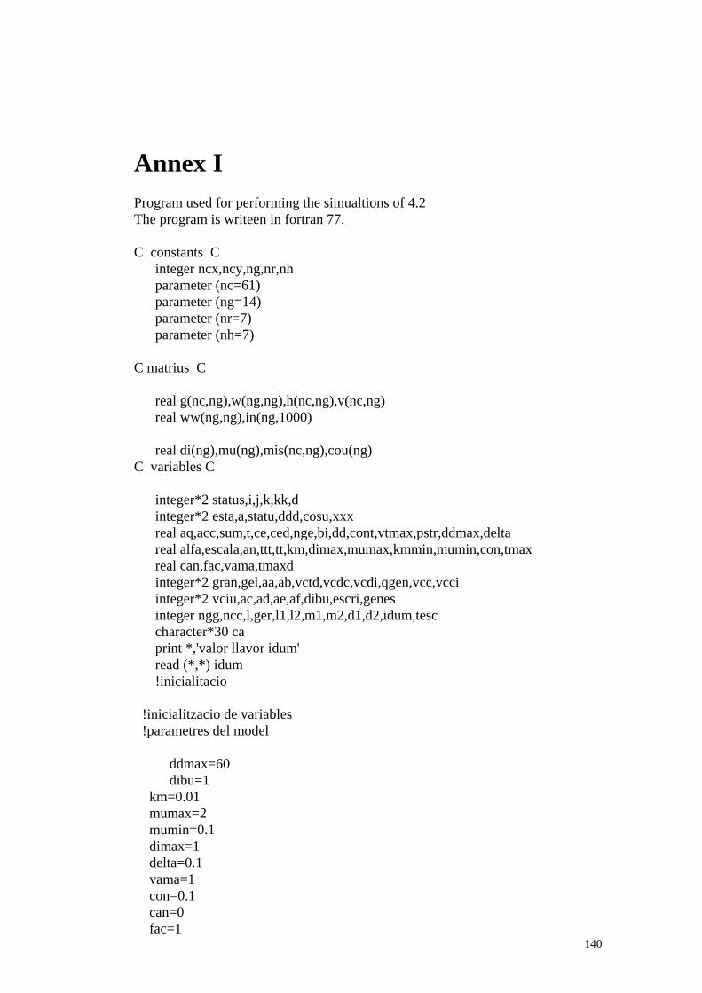
140

Annex I Program used for performing the simualtions of 4.2 The program is writeen in fortran 77. C constants C integer ncx,ncy,ng,nr,nh parameter (nc=61) parameter (ng=14) parameter (nr=7) parameter (nh=7) C matrius C real g(nc,ng),w(ng,ng),h(nc,ng),v(nc,ng) real ww(ng,ng),in(ng,1000) real di(ng),mu(ng),mis(nc,ng),cou(ng) C variables C integer*2 status,i,j,k,kk,d integer*2 esta,a,statu,ddd,cosu,xxx real aq,acc,sum,t,ce,ced,nge,bi,dd,cont,vtmax,pstr,ddmax,delta real alfa,escala,an,ttt,tt,km,dimax,mumax,kmmin,mumin,con,tmax real can,fac,vama,tmaxd integer*2 gran,gel,aa,ab,vctd,vcdc,vcdi,qgen,vcc,vcci integer*2 vciu,ac,ad,ae,af,dibu,escri,genes integer ngg,ncc,l,ger,l1,l2,m1,m2,d1,d2,idum,tesc character*30 ca print *,'valor llavor idum' read (*,*) idum !inicialitacio !inicialitzacio de variables !parametres del model ddmax=60 dibu=1 km=0.01 mumax=2 mumin=0.1 dimax=1 delta=0.1 vama=1 con=0.1 can=0 fac=1

141

!variables de visualitzacio escri=0 genes=0 tesc=0 !3D tmax=5. !/delta tmaxd=1 vtmax=2000. an=0.5 escala=2 l=4 ger=4 vctd=0 !variable per 3D, 1 aleshores 3D !altres vcdc=0 !variable per dibuix continu vcdi=0 !variable per dibuixa per sobre vcc=0 vcci=1 !tipus de ci vciu=1 pstr=40 !altres tontos ngg=ng ncc=ncx d=1 p=1 bi=0.25 esta=16 ttt=0 if (dibu.eq.1) call inici() C ci´ C 40 cosu=0 t=0 tt=0 ttt=ttt+1 g=0. h=0. w=0. vtmax=600 aq=ran2(idum) dd=ddmax*aq C a rel tenim quina hormona afecta a cada receptor, ho fem bijectivament C alfa=0.6 do i=1,ng,1 do j=1,ng,1 if (ran2(idum).gt.alfa) go to 203 aq=ran2(idum) if (aq.gt.bi) then

142

acc=1 else acc=-1 end if w(i,j)=ran2(idum)*acc 203 end do end do w=0 ww=0 !xarxa amb la que treball w(8,8)=ran2(idum) w(1,8)=ran2(idum) w(2,8)=ran2(idum) w(3,8)=ran2(idum) w(4,8)=ran2(idum) w(5,8)=ran2(idum) w(6,8)=ran2(idum) w(7,8)=ran2(idum) w(9,1)=ran2(idum) w(9,2)=-ran2(idum) w(10,3)=ran2(idum) w(10,9)=-ran2(idum) w(11,4)=ran2(idum) w(11,10)=-ran2(idum) w(12,5)=ran2(idum) w(12,11)=-ran2(idum) w(13,6)=ran2(idum) w(13,12)=-ran2(idum) w(14,7)=ran2(idum) w(14,13)=-ran2(idum) do i=1,ng di(i)=ran2(idum)*1 mu(i)=ran2(idum)*a end do do i=nh+1,ng di(i)=0 end do a=0 !condicions inicials 800 if (vcci.eq.1) then do i=1,nc do j=1,ng g(i,j)=ran2(idum) end do end do end if

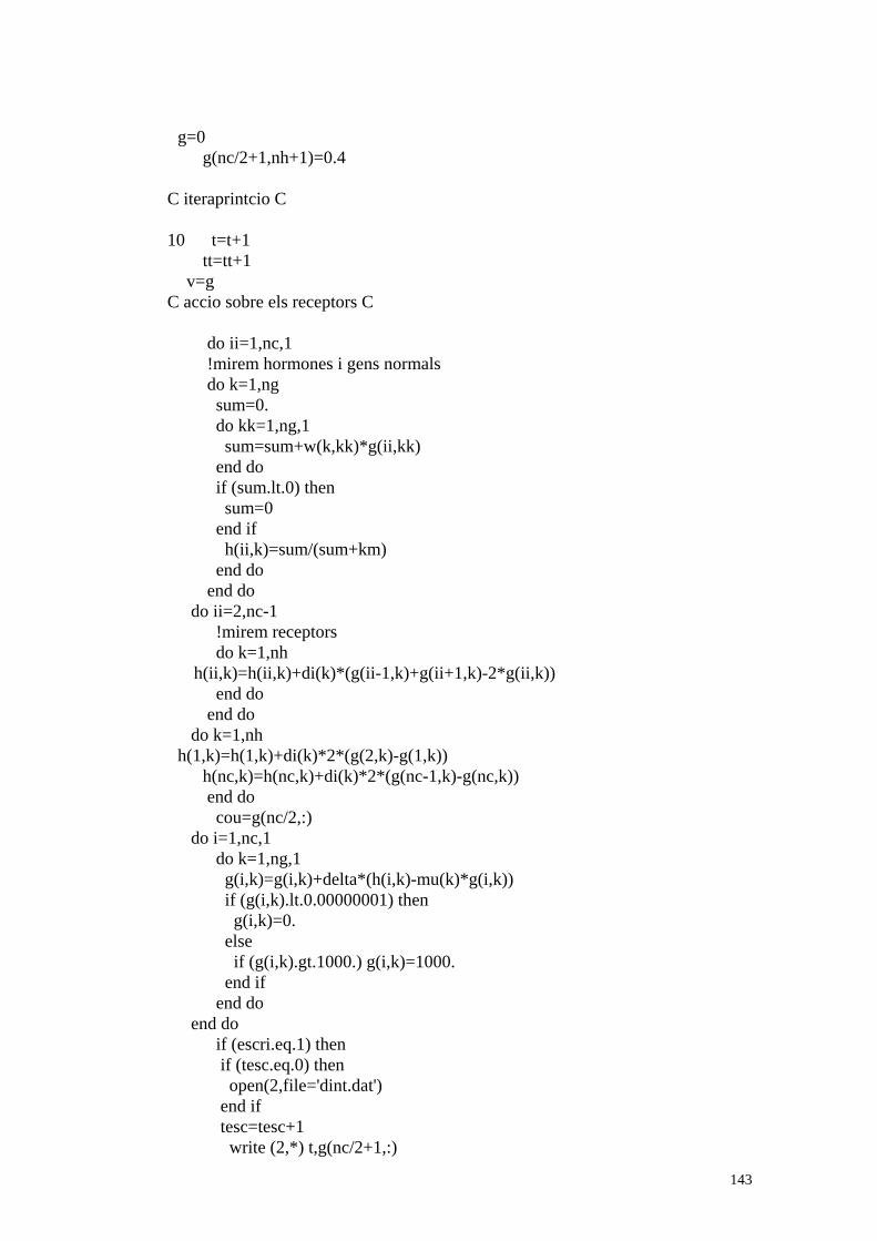
143

g=0 g(nc/2+1,nh+1)=0.4 C iteraprintcio C 10 t=t+1 tt=tt+1 v=g C accio sobre els receptors C do ii=1,nc,1 !mirem hormones i gens normals do k=1,ng sum=0. do kk=1,ng,1 sum=sum+w(k,kk)*g(ii,kk) end do if (sum.lt.0) then sum=0 end if h(ii,k)=sum/(sum+km) end do end do do ii=2,nc-1 !mirem receptors do k=1,nh h(ii,k)=h(ii,k)+di(k)*(g(ii-1,k)+g(ii+1,k)-2*g(ii,k)) end do end do do k=1,nh h(1,k)=h(1,k)+di(k)*2*(g(2,k)-g(1,k)) h(nc,k)=h(nc,k)+di(k)*2*(g(nc-1,k)-g(nc,k)) end do cou=g(nc/2,:) do i=1,nc,1 do k=1,ng,1 g(i,k)=g(i,k)+delta*(h(i,k)-mu(k)*g(i,k)) if (g(i,k).lt.0.00000001) then g(i,k)=0. else if (g(i,k).gt.1000.) g(i,k)=1000. end if end do end do if (escri.eq.1) then if (tesc.eq.0) then open(2,file='dint.dat') end if tesc=tesc+1 write (2,*) t,g(nc/2+1,:)

144

if (tesc.eq.1200) then close(1) escri=0 end if end if if (dibu.eq.1) then !56 call color(i+2) call color(0) call qua(45,65,70,75) call escriu(50,70,int(t)) end if C CONTROL CONTROL CONTROL CONTROL CONTROL CONTROL C CONTROL CONTROL CONTROL CONTROL CONTROL CONTROL C CONTROL CONTROL CONTROL CONTROL CONTROL CONTROL if (vcdc.eq.1) then call bujocel(g,ng,nc) end if ! ARA PREGUNTA 34 if (tt.gt.vtmax) then if (dibu.eq.1) then if (vcc.eq.1) call borrar() end if call borrar() call bujocel(g,ng,nc,-30,0) do i=1,ng do j=1,nc a=0 do k=1,nc if (g(j,i).gt.g(k,i)) a=a+1 end do mis(j,i)=a end do end do mis=mis/30 call bujocel(mis,ng,nc,-30,100) 6000 if (dibu.eq.1) call escriu(10,100,100) read (*,*) ac if (dibu.eq.1) then call color(0) call qua(0,90,20,120) end if if (ac.eq.2) go to 50 if (ac.eq.3) go to 40

145

vtmax=ac tt=0 vciu=1 end if !tt tmax if (ac.eq.44) then g=0.4 go to 10 end if if (ac.eq.4) then g=0 g(1,1)=1 go to 10 end if if (ac.eq.5) then open (1,file='reg.dat',access='append') do i=1,ng do j=1,ng if (w(i,j).ne.0) write (1,*) i,j,w(i,j) end do end do do i=1,ng write (1,*) i,di(i),mu(i) end do write (1,*) idum do i=1,nc write (1,*) i,g(i,:) end do close (1) end if if (ac.eq.6) then read (*,*) delta go to 6000 end if if (ac.eq.7) then if (escri.eq.0) then escri=1 else escri=0 end if tesc=0 go to 6000 end if go to 10 50 if (dibu.eq.1) call fi() end subroutine bujocel(g,ng,nc,x,y)

146

integer i,j,k,jj,ng,ncc,ng,x,y real g(nc,ng) !call borrar() do i=1,nc do k=1,ng call color(k) call punt(x+i+nc*k,y+int(200-g(i,k)*5)) !call punt(i*4+nc*4*k+1,int(200-g(i,k)*30)) !call punt(i*4+nc*4*k+2,int(200-g(i,k)*30)) !call punt(i*4+nc*4*k+3,int(200-g(i,k)*30)) end do end do

end subroutin

147

Annex II: Program used for the simulations in 5.2: selection simulations C EGRD.for !!!!!!!!!!!!!DIFUSIU!!!!!!!!!!!!!!!!!!!! C Definicions !parametres integer p,nc,ngmax parameter (p=100) !tamany de la poblacio:HA DE SER PARELL parameter (nc=25) !numero de celules parameter (ngmax=20) !DELTA,tes i dd esta a una subrutina PAS !matrius de veritat real g(p,nc,ngmax),fitt(p),gop(nc),fit(ngmax),me(p),fitu(p) real w(p,ngmax,ngmax),di(p,ngmax),rfitt(p),muu(p,ngmax) integer ng(p),nr(p),nh(p),des(p),mis(p,nc,ngmax) integer dess(p),miss(nc,ngmax),gooop(nc,1) integer si(p,ngmax),ming(p),goop(nc),ll(p),miso(nc) !matrius de visualitzacio !integer sc(p,0:llmax) !sumacio de color per a distingir els mutants !matrius tontes !matrius alocatables real mui(ngmax),dii(ngmax),gg(nc,ngmax),wg(ngmax,ngmax) real estable(nc,ngmax,2) !real, dimension(:), allocatable ::mui,dii !real, dimension(:,:), allocatable ::gg,wg !real, dimension(:,:,:), allocatable ::estable !variables importants real frc,inc,km,afie real mu !freq de nutacio real rangmax !variacio maxima en la freq de mutacio real consta !realcio entre la energia de fit i el cost real delta !variables contador real t,tes real gen,genn !variables de visualitzacio integer gran,npp !individus per pagina integer npx,npy,disx,dis integer dibu !variables de desicio integer guar,guard,vd !variables mesura real fittmax,fittmaxa !variables tontas integer testa,ngd,pd,nga integer testam !temps a aprtir del que mirem real temp !temps per visualitzacio real tedi !temps per dibuixos real cost,fitot

148

real a,b,c,algc,tt integer i,idum,aidum,j,k,it,ii,jj,kk,iii,jjj,kkk,ngg,nhg,nrg integer x,y integer ncc,pp character*30 ca character*8 cc common /ppncc/ pp,ncc common /kmdelta/ km,delta C Inicialitzacio !no de variables 22 idum=-16451001 !!print *,'idum' !read (*,*) idum if (idum.gt.0) go to 22 aidum=idum !open (2,file='dinfit2.dad',access='sequential') !CALL SETTEXTWINDOW(25,45,60,90) !status = SETWINDOW(.FALSE., 1, 200, 500, 200) !call outtext('aqui') !call seed(-1) dibu=0 !1 per dibuixar !if (dibu.eq.1) call inici(4) !call esperar() !IMPORTANTS !IMPORTANTS !IMPORTANTS !IMPORTANTS afie=100000 !afinament en la estabilitat(numero d'0=decimals) delta=0.1 km=0.1 !parametrer global mu=0.02 !freq. de mutacio per gen fmp=0.7 !part de mu que correspon a mutacions puntuals fn=0.4 !part de aquestes mutacions puntuals que son nous enh fd=0.1 !part que correspon a duplicacions fr=1-fd-fmp !part que correspon a recombinacions rangmax=1 !valor maxim del canvi per mutacio puntual frc=100. inc=100. tes=4000 !temps per a des testa=50 !temps max entre mires de estabilitat(el temps es alea) testam=200 !temps a partir del qual mirem l'estabilitat consta=1 !parametre xungu !de visualitzacio temp=1000000 tedi=1 disx=5 pp=p dis=5 !sc=0 !variables de visualitzacio gran=2

149

npp=pp npx=10 npy=19 !variables de desicio guar=0 !1 per guardar w i g a t=tedi guard=0 vd=0 !tontes ncc=nc gen=0 genn=0 tt=testa/2 !de llinatges !ng nr i nh do i=1,p ng(i)=6 nr(i)=3 nh(i)=3 end do !patro optim gop(1)=0.1 gop(2)=0.1 gop(3)=0.2 gop(4)=0.4 gop(5)=0.2 gop(6)=0.1 gop(7)=0.1 gop(8)=0.1 gop(9)=0.2 gop(10)=0.4 gop(11)=0.2 gop(12)=0.1 gop(13)=0.1 gop(14)=0.1 gop(15)=0.2 gop(16)=0.4 gop(17)=0.2 gop(18)=0.1 gop(19)=0.1 gop(20)=0.1 gop(21)=0.2 gop(22)=0.4 gop(23)=0.2 gop(24)=0.1 gop(25)=0.1 do i=1,nc jj=0 do j=1,nc if (gop(i).ge.gop(j)) jj=jj+1 end do goop(i)=jj

150

end do do i=1,nc !!print *,goop(i) end do !generacio de w !do i=1,p ! a=ran2(idum) ! w(i,nh(i)+1,nh(i)+1)=a ! a=ran2(idum) ! w(i,1,nh(i)+1)=a ! do j=1,ng(i) ! a=ran2(idum) ! w(i,j,j)=a*a ! a=ran2(idum) ! w(i,j,nh(i)+1)=a ! end do !end do w=0 !generacio de di do i=1,p do j=1,nh(i) a=ran2(idum) di(i,j)=a end do do j=1,ng(i) a=ran2(idum) muu(i,j)=a end do end do C Generacio !canvi de patro optim? !******************************************************************* ! FASE DE DESENVOLUPAMENT !******************************************************************* 10 gen=gen+1 genn=genn+1 print *,genn !!call escriu(550,250,int(genn)) fitt=0.1 !call clearscreen($GTEXTWINDOW) !condiciones inicials g=0. si=0 do i=1,p g(i,nc/2+1,nh(i)+1)=1. end do !!print *,int(genn),' generacio'

151

!if (genn/frc.eq.aint(genn/frc)) call canvipat(gop,nc) do iii=1,p !allocate(gg(1:nc,1:ng(iii))) !allocate(wg(1:ng(iii),1:ng(iii))) !allocate(dii(1:ng(iii))) !allocate(mui(1:ng(iii))) !allocate(estable(1:nc,1:ng(iii),1:2)) gg(:,:)=g(iii,:,:) wg(:,:)=w(iii,:,:) dii(:)=di(iii,:) mui(:)=muu(iii,:) ngg=ng(iii) nhg=nh(iii) nrg=nr(iii) estable=0 !iteracio do it=1,testam t=it !PAS call pas(gg,wg,dii,mui,ngg,nhg,nrg,ncc,ngmax) !PAS end do !testam estable(:,:,1)=0 !iteracio mirant l'estabilitat do it=1,tes-testam t=it !PAS call pas(gg,wg,dii,mui,ngg,nhg,nrg,ncc,ngmax) !PAS !posicionament del dibuix segons l'individu if (t/tt.eq.aint(t/tt)) then a=ran2(idum) tt=int(a*testa)+10 do j=1,ngg do i=1,nc estable(i,j,2)=gg(i,j) if (estable(i,j,1).ne.estable(i,j,2)) then do k=i,nc estable(k,j,1)=gg(k,j) end do si(iii,j)=0 go to 20 end if estable(i,j,1)=estable(i,j,2) end do si(iii,j)=1 20 end do !j !mirem si tots son estables per a sortir i estalbiar temps !!print *,t,si(iii,1),si(iii,2) !pause do i=1,ngg

152

if (si(iii,i).eq.0) go to 30 end do go to 40 30 end if end do !tes !mirem si en tenim algun estable fitt(iii)=0 !PER DEVANT !guardem els que son estables de si a estable 40 do i=1,nc do j=1,ng(iii) g(iii,i,j)=gg(i,j) end do end do !deallocate(gg) !deallocate(wg) !deallocate(dii) !deallocate(mui) !deallocate(estable) !!print *,t end do !iii !!call escriu(470,250,int(genn)) C !******************************************************************* ! FASE DE SELECCIO !******************************************************************* print *,'sele' do iii=1,p ngg=ng(iii) if (fitt(iii).ne.0) then !A !calcul de fit do i=1,ngg fit(i)=0 if (si(iii,i).eq.1) then !B do ii=1,nc kk=0 do jj=1,nc if (g(iii,ii,i).ge.g(iii,jj,i)) kk=kk+1 end do mis(iii,ii,i)=kk end do do j=1,nc fit(i)=fit(i)+abs(goop(j)-mis(iii,j,i)) end do else fit(i)=1000000 end if !B end do ! ara em de mirar quin es el minim

153

a=fit(1) do j=1,ngg if (fit(j).le.a) then ming(iii)=j a=fit(j) end if end do if (fitt(iii).ne.0.and.fit(ming(iii)).ne.0)then fitt(iii)=nc**2-fit(ming(iii)) else fit(iii)=0 end if if (fitt(iii).le.0) fitt(iii)=0 end if !A 70 end do !iii !ara calculem les fitness relatives !!print *,'sele A' a=0 fitu=fitt do iii=1,p a=a+fitt(iii) end do do iii=1,p fitt(iii)=fitt(iii)/a end do fitot=a rfitt=0 des=0 !call dinfit(fitu,genn) !call pintafreq(fitu) !repartim la descendencia a=0 b=p call ordena(fitt,pp,me) fittmax=fitu(int(me(p))) !!call escriu(500,200,int(fittmax)) !do i=p,1,-1 ! des(me(i))=int(p*fitt(me(i))) ! a=des(me(i))+a ! if (des(me(i)).gt.p.or.des(me(i)).lt.0) des(i)=0 !end do !do i=1,p ! c=des(me(i)) ! rfitt(me(i))=fitt(me(i))-(c/b) !end do !distribucio dels residus !call ordena(rfitt,pp,me) !do i=p,a+1,-1 ! des(me(i))=des(me(i))+1 !end do !call ordena(fitt,pp,me)

154

! ara els b ultims passen fills als b primers !SISTEMA DE SELECCIO RICARD-RADICAL des=0 a=0 do i=p/2+1,p des(int(me(i)))=2 a=a+des(int(me(i))) end do print *,'sele des' !end do !do j=1,b ! do i=1,p ! if (des(me(i)).ge.1) then ! des(me(i))=des(me(i))-1 ! go to 352 ! end if ! end do !352 end do 351 a=0 ll=0 do i=1,p if (des(i).ge.1) then ll(i)=1 des(i)=des(i)-1 end if end do !COPIA do iii=1,p do jjj=1,des(iii) do j=1,p if (ll(j).eq.0) then !mirem que els substituits no siguin iguals per a fer mes facil la filo ! if (ng(iii).ne.ng(j)) go to 130 ! do i=1,ng(j) ! do jj=1,ng(j) ! if (w(iii,i,jj).ne.w(j,i,jj)) go to 130 ! end do ! if (di(iii,i).ne.di(j,i)) go to 130 ! if (muu(iii,i).ne.muu(j,i)) go to 130 ! end do ! go to 120 !130 ng(j)=ng(iii) ll(j)=1 fitu(j)=fitu(iii) nh(j)=nh(iii) nr(j)=nr(iii) w(j,:,:)=w(iii,:,:) di(j,:)=di(iii,:) muu(j,:)=muu(iii,:) !sc(j,gen)=sc(iii,gen)

155

go to 120 end if end do 120 end do end do print *,'escriu' !write (2,*) fittmax,genn !print *,'kk' !******************************************************************* ! FASE DE MUTACIO !****************************************************************** !!print *,'mu' do iii=1,p do kkk=1,ng(iii) a=ran2(idum) if (a.lt.mu) then a=ran2(idum) !mutacio puntual if (a.lt.fmp) then 80 if (ii.lt.nh(iii)) then if (a.lt.0.25) then a=ran2(idum) a=rangmax-a*rangmax*2 di(iii,kkk)=di(iii,kkk)+a go to 140 end if if (a.gt.0.75) then a=ran2(idum) a=rangmax-a*rangmax*2 muu(iii,kkk)=muu(iii,kkk)+a go to 140 end if end if a=ran2(idum) jjj=int(a*ng(iii))+1 a=ran2(idum) if (a.gt.fn.and.w(iii,kkk,jjj).eq.0) go to 80 a=ran2(idum) a=rangmax-a*rangmax*2 w(iii,kkk,jjj)=w(iii,kkk,jjj)+a 140 a=ran2(idum) a=aint(a*16)+1 !sc(iii,gen)=sc(iii,gen-1)+a a=0 end if !puntu

156

!duplicacions o delecions(50% cadascuna) if (a.gt.fmp.and.a.lt.fmp+fd.and.ng(iii).lt.ngmax) then !tamany de la duplicacio exponenecial negativa a=ran2(idum) if (a.gt.0.5) then !duplicacio !PENDENT DE REVISIO DE SI PETA a=ran2(idum)**2.5 ngd=int(a*ng(iii))+1 a=ran2(idum) !posicio del primer duplicant pd=a*(ng(iii)-ngd) nga=ng(iii) !ng anterior ng(iii)=ng(iii)+ngd do i=pd,pd+ngd if (nh(iii).lt.i) then nr(iii)=nr(iii)+1 else nh(iii)=nh(iii)+1 end if do jj=ng(iii),i+1,-1 w(iii,jj,:)=w(iii,jj-1,:) w(iii,:,jj)=w(iii,:,jj-1) di(iii,jj)=di(iii,jj-1) muu(iii,jj)=muu(iii,jj-1) end do end do else !delecio do jj=kkk,ng(iii)-1 w(iii,jj,:)=w(iii,jj+1,:) w(iii,:,jj)=w(iii,:,jj+1) di(iii,jj)=di(iii,jj+1) muu(iii,jj)=muu(iii,jj+1) end do ng(iii)=ng(iii)-1 !si hem copiat una hormona if (kkk.lt.nh(iii)) nh(iii)=nh(iii)-1 a=ran2(idum) a=aint(a*16)+1 !sc(iii,gen)=sc(iii,gen-1)+a a=0 end if end if !dupl del !recombinacions if (a.gt.fmp+fd) then !reco a=ran2(idum) i=int(a*ng(iii))+1 !numero de e afectats per la recomb a=ran2(idum) kk=int(a*ng(iii))+1 !gen receptor do j=1,i !si es repeteixen els agafats no passa res eixi tenim a=ran2(idum)!exponencial negativa ii=int(a*ng(iii))+1

157

a=ran2(idum)!exponencial negativa jj=int(a*ng(iii))+1 a=w(iii,kkk,ii) w(iii,kkk,ii)=w(iii,kk,jj) w(iii,kk,jj)=a end do end if !reco end if end do end do !******************************************************************* ! FASE DE CONTROL !******************************************************************* if (dibu.eq.1) then !call color(0) !call qua(0,0,640,360) !call dinfit(fitu,genn) call pintafreq(fitu) !call escriu(550,250,int(genn)) !call escriu(500,200,int(fittmax)) end if print *,'con' if (fittmaxa.lt.fittmax) go to 333 !if (genn/tedi.eq.aint(genn/tedi))then 333 if (dibu.eq.1) then do iii=1,p i=int(me(iii)) !posicionament del dibuix segons l'individu y=int((iii-1)/npx) x=iii-y*npx x=x-1 ngg=ng(i) miss(:,:)=mis(i,:,:) if (si(i,ming(i)).eq.1) then call bujo(miss,ncc,ngg,gran,x,y,ming(i)) !dibuixem la fitness call bujfit(fitu,i,x,y,gran,npx) end if end do gooop=0 gooop(:,1)=goop(:) call bujo(gooop,ncc,1,gran,x,y+1,1) end if print *,dibu a=gen-llmax !pintem la filogenia

158

!if (a.lt.1) a=1 !do b=a,gen !call filogen(ll,b,dis,pp,disx,sc,a) !end do !**************************************************************************** ! HEM TINGUT PROGRES !**************************************************************************** !ara guardem el w i g de cada individu if (fittmax.ge.(nc**2)-3) go to 50 if (fittmaxa.lt.fittmax) then fittmaxa=fittmax do iii=p,p k=int(me(iii)) dii=di(k,:) mui=muu(k,:) wg=w(k,:,:) miso(:)=mis(k,:,ming(k)) write (ca,*) -aidum,'4p.dat' open (1,file=ca) write (1,*) aidum,genn,pp,nc write (1,*) iii,ng(k),nh(k),nr(k) write (1,*) fitu(k),ming(k),km write (1,*) delta,afie,ngmax write (1,*) tes,testam,testa do i=1,ng(k) write (1,*) dii(i),mui(i) end do do i=1,nc write(1,*) g(k,i,ming(k)),goop(i) end do write (1,*) 0,ming(k) do i=1,ng(k) do j=1,ng(k) if (w(k,i,j).ne.0) write (1,*) i,j,w(k,i,j),w(k,i,j) end do end do do i=1,nc write (1,*) mis(k,i,ming(k)),mis(k,i,ming(k)) end do !read (*,*) !call remor(wg,dii,mui,nc,ng(iii),nh,nr,tes,testa,+ !+testam,ming(k),ngmax,miso,aidum) print *,'ko' end do end if fittmaxa=fittmax if (genn.eq.temp) then C 90 if (dibu.eq.1) call fi() !!print *,'que fem'

159

!read (*,*) temp 90 tedi=temp+genn if (temp.eq.7) then !!print *,'opcions, 111 per canviar t de visualitzacio,222 per' !!print *,'veure ng per individu, 333 veure w de un individu' !!print *,'444 veure fitt de un ind.,555 veure g i mis de ind.' !!print *,'888 canviar gran, 999 per guardar 10 primers( s fit)' !!print *,'1111 canviar dis, 2222 canviar disx,3333 dibuixar els' !!print *,'valors reals de g, 4444 per ordenar el bujo segons la' !!print *,'la fitness, 5555 demanar l ordre' go to 90 end if if (temp.eq.111) then !call outtext('nou tedi') read (*,*) tedi tedi=tedi+genn !call outtext('nou temp') read(*,*) temp end if if (temp.eq.222) then do i=1,p/3 !!print *,i,ng(i) end do !pause do i=p/3+1,2*p/3 !!print *,i,ng(i) end do !pause do i=2*p/3+1,p !!print *,i,ng(i) end do go to 90 end if if (temp.eq.333) then !call outtext('quin individu') !read(*,*) iii do i=1,ng(iii) do j=1,ng(iii) !!print *,i,j,w(iii,i,j) end do !pause end do go to 90 end if if (temp.eq.444) then !call outtext('quin individu') read(*,*) iii !!print *,iii,ming(iii),fitt(iii) go to 90 end if if (temp.eq.555) then

160

!call outtext('quin individu') read(*,*) iii do i=1,nc !!print *,i,g(iii,i,ming(iii)),mis(iii,i,ming(iii)) end do go to 90 end if if (temp.eq.666) then vd=1 go to 90 end if if (temp.eq.777) then !call outtext('quin individu') read(*,*) iii do i=1,nc j=mis(iii,i,ming(iii)) !!print *,j,goop(i),abs(j-goop(i)) end do go to 90 end if if (temp.eq.888) then !!print *,'vell valor',gran,'nou valor ?' read (*,*) gran go to 90 end if if (temp.eq.999) then if (guar.eq.1) then guar=0 else guar=1 !!print *,'nom del fitxer?' read(*,*) ca end if go to 90 end if if (temp.eq.1111) then !!print *,'vell valor',dis,'nou valor ?' read (*,*) dis go to 90 end if if (temp.eq.2222) then !!print *,'vell valor',disx,'nou valor ?' read (*,*) disx go to 90 end if if (temp.eq.5555) then !call ordena(fitt,pp,me) !!print *,'quin ordre vosl veure' read(*,*) i !!print *,me(i) go to 90

161

end if temp=temp+genn end if go to 10 50 end !END !END !END !END !END !END !END !END !END !END !END !END !END !END !END !END !END !END !END !END !END !END !END !END !END !END !END !END !END !END !END !END !END !END !END !END !END !END !END !END !END !END !END !END !END !END !END !END !END !END !END !END !END !END !END !END !END !END !END !END subroutine pas(g,w,di,mu,ng,nh,nr,nc,ngmax) real delta integer nc,ng,nr,nh,ngmax real g(nc,ngmax),h(nc,ngmax) real w(ngmax,ngmax),di(ngmax),mu(ngmax) !variables importants real dd,km !variable tontes real sum,t,gen integer i,k,ii,kk integer*2 aa,ab,l1,l2 common /kmdelta/ km,delta !variables importants ini dd=1 do ii=1,nc,1 !mirem hormones i gens normals do k=1,ng sum=0. do kk=1,ng,1 sum=sum+w(k,kk)*g(ii,kk) end do if (sum.lt.0) then sum=0 end if h(ii,k)=sum/(sum+km) end do end do do ii=2,nc-1 !mirem receptors do k=1,nh h(ii,k)=h(ii,k)+di(k)*(g(ii-1,k)+g(ii+1,k)-2*g(ii,k)) end do end do

162

do k=1,nh h(1,k)=h(1,k)+di(k)*2*(g(2,k)-g(1,k)) h(nc,k)=h(nc,k)+di(k)*2*(g(nc-1,k)-g(nc,k)) end do do i=1,nc,1 do k=1,ng,1 g(i,k)=g(i,k)+delta*(h(i,k)-mu(k)*g(i,k)) end do end do end subroutine pas subroutine canvipat(gop,nc) !A FEEEEEEEEEEEEER integer i,nc real a real gop(nc) a=ran2(idum) i=int(a*nc)+1 a=ran2(idum) a=1-2*a gop(i)=gop(i)+a end subroutine canvipat subroutine bujo(mis,nc,ng,gran,x,y,min) integer nc,ng integer mis(nc,ng) integer iii,i,j,k,kk,gran,xmin,ymin,xmax,ymax,x,y integer dx,dy,ming integer a,min real b dx=(nc+2)*gran dy=nc+5 !determinem la posicio segons l'individu xmin=(nc/2)*gran+x*dx xmax=nc*8/5*gran+x*dx ymin=2*gran+y*dy ymax=14*gran+y*dy dx=xmax-xmin dy=ymax-ymin !call color(ng) if (ng.eq.1) then !call color(5) end if !call color(ng) !status=rectangle($GBORDER,xmin,ymin,xmax,ymax) !call linia(xmin,ymin,xmax,ymin)

163

!call linia(xmin,ymax,xmax,ymax) !call linia(xmin,ymin,xmin,ymax) !call linia(xmax,ymin,xmax,ymax) !do i=1,ng,1 ! do j=1,nc,1 ! !call color(i*a) ! do k=1,gran ! do kk=1,gran !!call punt(xmin+(j-1)*gran+kk,ymax-mis(j,i)*dy/nc) ! end do ! end do ! end do !end do !call color(min) do j=1,nc,1 do k=1,gran do kk=1,gran !call punt(int(xmin+(j-1)*gran+kk),int(ymax-mis(j,min)*dy/nc)) end do end do end do 10 end subroutine bujo subroutine bujfit(fitt,iii,x,y,gran,npx) integer pp,ncc real fitt(pp) integer iii,gran,x,y,xmin,ymin,xmax,ymax integer dx,dy common /ppncc/ pp,ncc !determinem la posicio segons l'individu !call color(6) dx=(ncc+2)*gran dy=ncc+5 xmin=(ncc/2)*gran+x*dx xmax=ncc*8/5*gran+x*dx ymin=2*gran+y*dy ymax=14*gran+y*dy dx=xmax-xmin dy=ymax-ymin xmin=xmin+2 !call linia(xmin,ymax-1,xmin,int(ymax-1-fitt(iii)*dy/(ncc**2+10))) !call moveto(xmin+2,ymax-1,xy) !status=lineto(xmin+2,ymax-1-fitt(iii)*dy/(ncc**2+10)) end subroutine bujfit subroutine ordena(ma,rang,me) !agafa la matriu ma i la torna ordenada de major a menor integer rang,i,j,k real ma(rang),me(rang),mu(rang) real a

164

me=0 mu=0 do i=1,rang a=ma(i) b=1 do j=1,rang if (a.gt.ma(j)) b=b+1 end do mu(i)=b do j=b,rang if (me(j).eq.0) then me(j)=i go to 10 end if end do 10 end do end subroutine ordena subroutine dinfit(fitu,genn) integer i real genn,a,gen integer pp,ncc real fitu(pp) common /ppncc/ pp,ncc gen=genn if (genn/600.eq.aint(genn/600.)) then gen=0 !!call qua(0,300,600,480) end if do i=1,pp !call color(int(fitu(i)-int(fitu(i)/16)*16)) !call punt(int(gen),int(600-200*fitu(i)/(ncc**2))) end do do i=1,100 !call color(1) !call punt(i,479) end do end subroutine dinfit subroutine pintafreq(fitu) integer i,j integer pp,ncc real fitu(pp),f(pp) real me(pp) real genn,a common /ppncc/ pp,ncc !open (3,file='frefit.dad',access='append') !call color(0) !status=rectangle($GFILLINTERIOR,0,200,200,300)

165

!anem a veure quants tenim de cada cas f=0 do i=1,pp do j=1,pp if (fitu(i).eq.fitu(j)) then f(i)=f(i)+1 end if end do end do !do i=1,pp ! write (3,*) i,fitu(i),f(i) !end do !close(3) do i=1,pp if (f(i).ne.0) then !call color(i-int(i/16)*16) !call punt(int(100*fitu(i)/ncc**2),int(360-100*f(i)/p)) end if end do do i=50,150 !call color(2) !call punt(i,360) end do end subroutine pintafreq subroutine remor(w,di,muu,nc,ng,nh,nr,tes,testa,testam,min,ngmax, +miso,aidum) !variables entrants integer nc,ng,testa,testam,min,ngmax,aidum real tes real w(ngmax,ngmax) real di(ngmax),muu(ngmax) !variables propies integer si(ng),mis(nc),miso(nc) real genn,fitt,t integer it,tt,iii,i,j,k,ii,jj,kk,gmax,jjj integer nw,nww,cont integer gw(ng*ng,2) real muts(ng*ng) !integer, dimension(:,:), allocatable ::gw !real, dimension(:), allocatable ::muts real g(nc,ng),estable(nc,ng,2) character*30 ca tt=testa/2 !***************************************************************** ! CREACIO !*****************************************************************

166

!open (1,file='mod.dat',access='append') nw=0 cont=0 tt=0 mis=0 !allocate(gw(nw,2)) !allocate(muts(nw)) nw=0 do i=1,ng do j=1,ng if (w(i,j).ne.0.) then nw=nw+1 gw(nw,1)=i gw(nw,2)=j end if end do end do do i=1,nw muts(i)=w(gw(i,1),gw(i,2)) end do go to 50 ! MUTACIO EN SI: INICI 220 do jjj=1,3 do jj=1,4 nww=0 do iii=1,nw if (jj.eq.1) then if (w(gw(iii,1),gw(iii,2)).ne.0) then w(gw(iii,1),gw(iii,2))=0 else cycle end if else !dos veins if (w(gw(iii,1),gw(iii,2)).ne.0) then w(gw(iii,1),gw(iii,2))=0 do ii=iii,nw if (w(gw(ii,1),gw(ii,2)).ne.0) then w(gw(ii,1),gw(ii,2))=0 go to 230 else cycle end if end do 230 end if end if !MUTACION EN SI: FI !***************************************************************** ! DESENVOLUPAMENT !*****************************************************************

167

!!print *,iii g=0. g(nc/2+1,nh+1)=1. estable=0 do it=1,testam call pas(g,w,di,muu,ng,nh,nr,nc,ngmax) end do !testam do it=1,tes-testam t=it call pas(g,w,di,muu,ng,nh,nr,nc,ngmax) if (t/tt.eq.aint(t/tt)) then a=ran2(idum) tt=int(a*testa)+10 do j=1,ng do i=1,nc estable(i,j,2)=g(i,j) if (estable(i,j,1).ne.estable(i,j,2)) then do k=i,nc estable(k,j,1)=g(k,j) end do si(j)=0 go to 20 end if estable(i,j,1)=estable(i,j,2) end do si(j)=1 20 end do !j do i=1,ng if (si(i).eq.0) go to 30 end do go to 40 !FI ESTABILITAT 30 end if !testa end do !tes C******************************************************************** C VERIFICACIO C******************************************************************** !CALCUL MIS INICI 40 mis=0 if (si(min).eq.1) then do i=1,nc kk=0 do j=1,nc if (g(i,min).ge.g(j,min)) kk=kk+1 end do mis(i)=kk end do end if do i=1,nc

168

if (mis(i).ne.miso(i)) then if (jj.eq.1) then w(gw(iii,1),gw(iii,2))=muts(iii) go to 60 else w(gw(iii,1),gw(iii,2))=muts(iii) w(gw(ii,1),gw(ii,2))=muts(ii) go to 60 end if else nww=nww+1 end if end do 60 end do !iii !if (nww.eq.0) go to 50 end do !jj end do !jjj !FI CALCUL MIS 50 write (1,*) nw,min do i=1,nw write (1,*) gw(i,1),gw(i,2),w(gw(i,1),gw(i,2)),muts(i) end do do i=1,nc write (1,*) miso(i),mis(i) end do close(1) !deallocate (gw) !deallocate (muts) end subroutine remor

169

Program used for simulating concrete networks: !Fa simualnt xarxes de un determinat modul i apunta els n de mostres fetes ! el numero de patrons trobats i els patrons nous trobats ! Definicions !parametres integer nc,ng,o,nh,nr,rep parameter (ng=7) parameter (nr=3) parameter (nh=4) parameter (nc=25) !numero de celules parameter (o=19) parameter (rep=10000000) integer pa(100000,nc) !DELTA,tes i dd esta a una subrutina PAS !matrius de veritat real g(nc,ng),h(nc,ng) real w(ng,ng),di(nh),mu(ng) integer mis(nc) integer si(ng) integer min real estable(nc,ng,o) integer*2 aa,ab,l1,l2 !variables importants real km,sum real delta,npa,nit !variables contador real t,tes integer gen,mi !variables de desicio integer testa integer testam !temps a aprtir del que mirem real temp !temps per visualitzacio real tedi !temps per dibuixos real a,b,c integer i,idum,aidum,j,k,it,ii,jj,kk,iii,jjj,kkk,kkkk integer tt character*30 ca character*8 cc ! Inicialitzacio gen=1 !no de variables 22 idum=-222222 ca='gnedemgrsa2.dat' open (1,file=ca) delta=0.1 km=0.1 !parametrer global

170

tes=4000 !temps per a des testa=100 !temps max entre mires de estabilitat(el temps es alea) testam=200 !temps a partir del qual mirem l'estabilita write (1,*) nc,ng,nh,nr,o,tes,testa,testam,delta,km,rep tt=0 w=0. npa=0 nit=1 do kkkk=1,rep !print *,kkkk w(1,2)=ran2(idum) w(2,1)=ran2(idum) w(3,2)=ran2(idum) w(2,3)=ran2(idum) w(3,4)=ran2(idum) w(4,3)=ran2(idum) w(1,5)=-ran2(idum) w(2,6)=-ran2(idum) w(3,7)=-ran2(idum) w(5,1)=ran2(idum) w(6,2)=ran2(idum) w(7,3)=ran2(idum) w(1,6)=ran2(idum) w(2,7)=ran2(idum) w(3,5)=ran2(idum) !w(7,3)=ran2(idum) !generacio de di do j=1,nh di(j)=ran2(idum) end do do j=1,ng mu(j)=ran2(idum) end do ! Generacio !canvi de patro optim? !******************************************************************* ! FASE DE DESENVOLUPAMENT !******************************************************************* 10 g=0. g(13,1)=1. estable=0 !iteracio do it=1,testam

171

do ii=1,nc,1 !mirem hormones i gens normals do k=1,ng sum=0. do kk=1,ng,1 sum=sum+w(k,kk)*g(ii,kk) end do if (sum.lt.0) then sum=0. end if h(ii,k)=sum/(sum+km) end do end do do ii=2,nc-1 !mirem receptors do k=1,nh h(ii,k)=h(ii,k)+di(k)*(g(ii-1,k)+g(ii+1,k)-2*g(ii,k)) end do end do do k=1,nh h(1,k)=h(1,k)+di(k)*2*(g(2,k)-g(1,k)) h(nc,k)=h(nc,k)+di(k)*2*(g(nc-1,k)-g(nc,k)) end do do i=1,nc,1 do k=1,ng,1 g(i,k)=g(i,k)+delta*(h(i,k)-mu(k)*g(i,k)) if (g(i,k).lt.0.000001) g(i,k)=0. end do end do end do !testam estable(:,:,1)=0 do it=1,tes-testam t=it do ii=1,nc,1 !mirem hormones i gens normals do k=1,ng sum=0. do kk=1,ng,1 sum=sum+w(k,kk)*g(ii,kk) end do if (sum.lt.0) then sum=0. end if h(ii,k)=sum/(sum+km) end do end do do ii=2,nc-1 !mirem receptors

172

do k=1,nh h(ii,k)=h(ii,k)+di(k)*(g(ii-1,k)+g(ii+1,k)-2*g(ii,k)) end do end do do k=1,nh h(1,k)=h(1,k)+di(k)*2*(g(2,k)-g(1,k)) h(nc,k)=h(nc,k)+di(k)*2*(g(nc-1,k)-g(nc,k)) end do do i=1,nc,1 do k=1,ng,1 g(i,k)=g(i,k)+delta*(h(i,k)-mu(k)*g(i,k)) if (g(i,k).lt.0.000001) g(i,k)=0. end do end do !if (sum(g).eq.0.) then ! print *,sum(g),g(:,1) ! mi=0 ! go to 50 !end if a=t/testa if (a.ge.aint(a).and.a.lt.aint((t+o)/testa)) then tt=tt+1 do i=1,nc do j=1,ng estable(i,j,tt)=g(i,j) end do end do end if if (a.eq.aint((t+o)/testa)) then tt=0 si(:)=1 do i=1,ng do j=1,nc do ii=1,o do k=ii,o if (estable(j,i,ii).ne.estable(j,i,k)) then si(i)=0 go to 20 end if end do end do end do 20 end do do i=1,ng if (si(i).eq.0) go to 30 end do go to 40 30 end if end do !tes

173

40 do i=1,nc jj=0 do j=1,nc if (g(i,gen).ge.g(j,gen)) jj=jj+1 end do mis(i)=jj end do if (it.gt.3800) mit=0 mi=1 50 nit=nit+1 if (mi.eq.1) then !MIREM SI EL PATRO ES NOU k=0 do i=1,npa do j=1,nc if (pa(i,j).ne.mis(j)) then k=k+1 go to 58 end if end do 58 end do if (k.eq.npa) then npa=npa+1 pa(npa,:)=mis write (1,*) int(nit),mis end if end if end do !rep close(1) end !END !END !END !END !END !END !END !END !END !END !END !END !END !END !END !END !END !END !END !END !END !END !END !END !END !END !END !END !END !END !END !END !END !END !END !END !END !END !END !END !END !END !END !END !END !END !END !END

!END !END !END !END !END !END !END !END !END !END !END !EN

174

Annex III:

Program used for the tooth model: ' ' #################### ' ##### PROLOG ##### ' #################### ' PROGRAM "progname" ' 1-8 char program/file name without .x or any .extent VERSION "0.0000" ' version number - increment before saving altered program IMPORT "xma" ' Math library : SIN/ASIN/SINH/ASINH/LOG/EXP/SQRT... ' IMPORT "xcm" ' Complex library : complex number library (trig, etc) IMPORT "xst" ' Standard library : required by most programs ' IMPORT "xgr" ' GraphicsDesigner : required by GuiDesigner programs ' IMPORT "xui" ' GuiDesigner : required by GuiDesigner programs ' DECLARE FUNCTION Entry () DECLARE FUNCTION SINGLE RAND(ULONG) 'ATENCIO AFEGIM UNA CERTA FONDARIA PER CADA CONJUNT DE CEL.LULES QUE S'AFEGEIXEN ' ###################### ' ##### Entry () ##### ' ###################### ' FUNCTION Entry () 'DECLARACIONS DE VARIABLES 'matrius core DOUBLE DI[] 'cambra de difusio DOUBLE MEM[] DOUBLE FO[] 'fondaria del epiteli a diferents llocs UBYTE EXIS[] 'existencia o no de un cub de difusio DOUBLE DIF[] 'coeficients de difusio DOUBLE MU[] 'taxa de degradacio DOUBLE TDI[] 'temps per a la diferenciacio

175

UBYTE IR[] 'dif de les cels 'variables core SLONG NG 'numero de gens DOUBLE FPP 'factor de proporcionalitat entre mitosi i concentracio SLONG DELE 'delay en lectura DOUBLE TAHOR,MAXTAHOR 'taxa de creixement horitzontal QUE NO SIGUI MAJOR QUE 1 DOUBLE TAINCA 'taxa de increment de noves cel. ANTERIORMENT DOUBLE TAINCP 'POSTERIORMENT DOUBLE TAINCB 'BUCALMENT DOUBLE TAINCL 'LINGUALMENT DOUBLE TACRE,MAXTACRE 'taxa de creixement DOUBLE TBMX,TBRX,TBMY,TBRY 'taxes de creixement horintzontal, MX es I+1, RX es I-1, MY es J+1, RY es J-1 DOUBLE MMX,MRX,MMY,MRY 'maxim de creixement en cada direccio DOUBLE TIDI 'taxa de increment de diferenciacio DOUBLE UM 'umbral per comenc,ar diferenciacio DOUBLE UMM 'umbral per aturat mitosi DOUBLE UMH 'umbral de actuacio del inhibidor DOUBLE DIU,DID,MAXDID,MAXDIU 'difusio de un gen i del altre DOUBLE MUU,MUD 'taxes de degradacio DOUBLE TAVER 'temps de creixement vertical DOUBLE TADI 'temps per difusio DOUBLE DELTA 'constant de integracio DOUBLE ACAC,ACIH,IHAC,MAXACAC,MAXIHAC 'lo que toca ja se sab DOUBLE ACACA 'taxa per defecte de activacio de per si DOUBLE FA,FP,FB,FL,MAXFA,MAXFB,MAXFL,MAXFP DOUBLE KMU,KMD 'mikaelis SLONG NCELX,NCELY GIANT T 'temps del pas global GIANT TT 'temps de difusio 'parametres de implementacio DOUBLE TADIX,TADIY,TADIZ 'tamany del espai de difusio en unitats comparables a les de forma 'llavor DOUBLE LLAVOR 'de visualitzacio SLONG TAXDI,TAYDI SLONG TAXFO,TAYFO SLONG IFXDI,IFYDI SLONG IFXFO,IFYFO SLONG NDIX,NDIY,NDIZ SLONG TEDE 'temps entre preguntes per defecte SLONG TBU 'temsp cada quan dibuixem

176

'de visualitzacio 3d SLONG L,LU,LD 'longitud de les unions DOUBLE AN 'angle de visualitzacio SLONG POSX,POSY,POSXU,POSYU,POSXD,POSYD 'coordinades de inici de la grafica DOUBLE ES,ESU,ESD'escala UBYTE REV 'rotacio o no 'transients DOUBLE PMAX DOUBLE H[] DOUBLE AMA[],VA[],AMB[] DOUBLE MEFO[],MEFOD[] DOUBLE AMIN UBYTE ESTATS[],ORD[] SLONG TE,CMEM SLONG UT,TLE 'ultim temps posat i temps a llegir XLONG FU,FT STRING file2$ 'per defecte SLONG I,J,K,II,JJ,KK,III,JJJ,KKK,IIII,JJJJ,KKKK,KKKKK,IJ,JI,TI,TM DOUBLE A,B,C,D,E,F,G,H,X,Y,Z,CC DOUBLE DPX,DPY,DMY,DMX DOUBLE DDPX,DDPY,DDMY,DDMX 'ASSIGNACIONS 'llavor LLAVOR=9 ' matrius core NDIX=30 : NDIY=30 : NDIZ=20 DEC NDIX : DEC NDIY : DEC NDIZ 'variables core NG=2 : DEC NG 'numero de gens DELE=2 'delay en la lectura FPP=1 'factor de proporcionalitat entre mitosi i concentracio 'intensitat de creixement vertical TAINCA=1 TAINCP=1 TAINCB=1 TAINCL=1 DELTA=0.05 'delta de integracio TADI=1.05 'temps per difusio 'inhibidor ACACA=0.001 ACIH=1 'efecte del inhibidor UMH=1 'umbral de actuacio del inhibidor

177

CC=1 aa: 'parametres de implemtacio TADIX=NDIX : TADIY=NDIY : TADIZ=NDIZ 'tamany del espai de difusio en unitats comparables a les de forma 'de visualitzacio TAXDI=800 : TAYDI=1000 TAXFO=150 : TAYFO=700 IFXDI=TAXFO+10 : IFYDI=40 IFXFO=0 : IFYFO=40 TEDE=12000 : TE=TEDE TBU=3000 'de visualitzacio 3d L=7 'longitud de les unions LU=5 : LD=LU AN=1 'angle de visualitzacio POSX=-80 'desplac,ament de la grafica en el eix horitzontal POSY=-30 'desplac,ament de la grafica en el eix vertical POSXU=10 POSYU=10 POSXD=POSXU POSYD=POSYU ES=L 'escala ESU=30/UMH :ESD=30/UMH REV=0 'rotacio o no 'transients DIM MEFO[NDIX,NDIY] AMIN=0.000000001 'DIMENSIONALITZACIONS 'matrius core DIM DI[NDIX,NDIY,NDIZ,NG],H[NDIX,NDIY,NDIZ,NG] 'cambra de difusio DIM EXIS[NDIX,NDIY,NDIZ] 'angle de visualitzacio DIM FO[NDIX,NDIY] 'coordinades de inici de la grafica DIM DIF[NG] 'coeficients de difusio DIM MU[NG] 'taxa de degradacio DIM TDI[NDIX,NDIY] 'temps per a la diferenciacio DIM IR[NDIX,NDIY,NDIZ] DIM MEM[NDIX,NDIY,DELE] DIM AMA[NDIX,NDIY],VA[3],AMB[NDIX,NDIY,3] DIM ESTATS[NDIX,NDIY,2],ORD[3] 'CONDICIONS INICIALS TRIVIALS 'CONDICIONS INICIALS

178

NCELX=2 NCELY=3 MAXTAHOR=0.001 MAXTACRE=0.001 MAXACAC=3 MAXIHAC=200 MAXDIU=1 MAXDID=1 MAXFA=0.001 MAXFP=0.001 MAXFL=0.001 MAXFB=0.001 'XstClearConsole() LLAVOR=4 FT=OPEN("/home/isaac/ddents/dent7.dat",$$RWNEW) WRITE [FT],LLAVOR,NDIX,NDIY,NDIZ,DELTA,MAXTACRE,MAXTAHOR,MAXACAC,MAXIHAC,MAXFA,MAXFB,MAXFP,MAXFL,MAXDIU,MAXDID,TEDE,TBU reinici: TAHOR=RAND(@LLAVOR)*MAXTAHOR TACRE=RAND(@LLAVOR)*MAXTACRE ACAC=RAND(@LLAVOR)*MAXACAC IHAC=RAND(@LLAVOR)*MAXIHAC 'activador DIU=RAND(@LLAVOR)*MAXDIU DID=RAND(@LLAVOR)*MAXDID FA=RAND(@LLAVOR)*MAXFA FP=RAND(@LLAVOR)*MAXFP FB=RAND(@LLAVOR)*MAXFB FL=RAND(@LLAVOR)*MAXFL WRITE [FT],TACRE,TAHOR,DIU,DID,FA,FB,FP,FL,ACAC,IHAC FOR I=0 TO NDIX FOR J=0 TO NDIY FOR K=0 TO NDIZ DI[I,J,K,1]=0 DI[I,J,K,0]=0 EXIS[I,J,K]=0 IR[I,J,K]=0 NEXT K AMA[I,J]=0 FO[I,J]=0 NEXT J NEXT I FOR I=NDIX/2-NCELX TO NDIX/2

179

FOR J=NDIY/2-NCELY TO NDIY/2 DI[I,J,0,1]=0.01 DI[I,J,0,0]=0 EXIS[I,J,0]=1 FO[I,J]=AMIN NEXT J NEXT I '**************************************************************************** ' PPPP RRRR OOOOO GGGG RRRR AAAAA MM MM AAAAA ' P P R R O O G R R A A M M M M A A ' PPPP RRRR O O G GG RRRR AAAAA M M M AAAAA ' P R R O O G G R R A A M M A A ' P R R OOOOO GGGG R R A A M M A A '***************************************************************************** KKKKK=0 T=0 TT=0 PMAX=AMIN iteracio: FOR KKKK=0 TO TE INC T INC TT GOSUB DIFUSIO GOSUB CREVER GOSUB REVISAR GOSUB CREHOR 'CREIXEMENT HORITZONTAL FOR I=1 TO NDIX-1 FOR J=1 TO NDIY-1 IF (FO[I,J]>=AMIN) THEN IF (FO[I+1,J]<AMIN) THEN AMA[I+1,J]=AMA[I+1,J]+FB END IF IF (FO[I-1,J]<AMIN) THEN AMA[I-1,J]=AMA[I-1,J]+FL END IF IF (FO[I,J+1]<AMIN) THEN AMA[I,J+1]=AMA[I,J+1]+FA END IF IF (FO[I,J-1]<AMIN) THEN AMA[I,J-1]=AMA[I,J-1]+FP END IF END IF NEXT J

180

NEXT I A=TT IF (A/TBU=INT(A/TBU)) THEN FOR I=0 TO NDIX FOR J=0 TO NDIY K=INT(FO[I,J]) IF (FO[I,J]>AMIN) THEN A=FO[I,J] : B=DI[I,J,K,0] : C=DI[I,J,K,1] WRITE [FT],I,J,A,B,C END IF NEXT J NEXT I I=TT WRITE [FT],I END IF NEXT KKKK GOTO reinici 'A$=INLINE$("") fi: '*************************************************************************************************** '**************************************************************************** ' SSSS U U BBBB SSSS ' S U U B B S ' SSSS U U BBBB SSSS ' S U U B B S ' SSSS UUUUU BBBB SSSS '***************************************************************************** '****************************************************** SUB CREVER 'EXSUB MITOSI: CREIXEMENT EN FUNCIO DE LA CONCENTRACIO FOR I=0 TO NDIX FOR J=0 TO NDIY KK=INT(FO[I,J]) A=0 IF (FO[I,J]>=AMIN) THEN B=DI[I,J,KK,1]'*DI[I,J,KK,0] A=TACRE*(UMH-B**FPP)

181

END IF IF (A>0) FO[I,J]=FO[I,J]+A IF (FO[I,J]>PMAX) THEN IF (PMAX<NDIZ) THEN PMAX=FO[I,J] ELSE PMAX=NDIZ END IF END IF JJ=INT(FO[I,J]) IF (JJ>KK) THEN IF (JJ>=NDIZ) THEN FO[I,J]=NDIZ JJ=NDIZ DI[I,J,JJ,0]=DI[I,J,KK,0] DI[I,J,JJ,1]=DI[I,J,KK,1] PMAX=FO[I,J] ELSE III=JJ-KK IF (III>=NDIZ) III=NDIZ IF (KK-1>0) THEN FOR K=INT(PMAX) TO JJ STEP -1 DI[I,J,K,0]=DI[I,J,K-III,0] DI[I,J,K,1]=DI[I,J,K-III,1] NEXT K ELSE FOR K=INT(PMAX) TO JJ STEP -1 IF (K-III>=0) THEN DI[I,J,K,0]=DI[I,J,K-III,0] DI[I,J,K,1]=DI[I,J,K-III,1] ELSE EXIT FOR END IF NEXT K END IF END IF END IF NEXT J NEXT I 'EXSUB ADDICIO: ADDICIO DE NOUS CUBS EN FUNCIO DE EL CRES 'ARA FEM EXISTIR ELS CUBS ENTRE LA FONDARIA A I PMAX I QUE TINGUIN CUBS EXISTENS A SOBRE FOR II=1 TO NDIX-1 FOR JJ=1 TO NDIY-1 IF (FO[II,JJ]>=AMIN) THEN KK=INT(FO[II,JJ]) FOR K=KK TO INT(PMAX) EXIS[II,JJ,K]=1 NEXT K

182

END IF NEXT JJ NEXT II 'EXSUB REDUDI: ELIMINACIO DELS CUBS FORA DE LA DENT FOR I=1 TO NDIX-1 FOR J=1 TO NDIY-1 IF (FO[I,J]>=1) THEN FOR K=0 TO INT(FO[I,J])-1 DI[I,J,K,0]=0 DI[I,J,K,1]=0 EXIS[I,J,K]=0 NEXT K END IF NEXT J NEXT I END SUB '****************************************************** '****************************************************** SUB REVISAR FOR I=1 TO NDIX-1 FOR J=1 TO NDIY-1 IF (FO[I,J]<1 && FO[I,J]<>0) GOTO bb NEXT J NEXT I 'ara anem a estalviar espai i passem tots els elements un punt amunt FOR I=0 TO NDIX FOR J=0 TO NDIY FOR K=0 TO NDIZ-1 DI[I,J,K,0]=DI[I,J,K+1,0] : DI[I,J,K,1]=DI[I,J,K+1,1] EXIS[I,J,K]=EXIS[I,J,K+1] IR[I,J,K]=IR[I,J,K+1] NEXT K IF (FO[I,J]<>0) FO[I,J]=FO[I,J]-1 NEXT J NEXT I bb: END SUB '****************************************************** '******************************************************

183

SUB CREHOR FOR I=0 TO NDIX FOR J=0 TO NDIY MEFO[I,J]=FO[I,J] NEXT J NEXT I 'AGAFEM UN PUNT I CALCULEM LES DISTANCIES DE AQUEST PUNT I ELS EXTREMS 'SEMPRE I QUAN ELS VEINS NO SIGUIN MES ALTS FOR I=1 TO NDIX-1 FOR J=1 TO NDIY-1 IF (FO[I,J]>=AMIN) THEN DPX=0 II=I DO INC II FOR K=INT(FO[II,J]) TO PMAX INC DPX NEXT K LOOP UNTIL (FO[II,J]<AMIN) DMX=0 II=I DO DEC II FOR K=INT(FO[II,J]) TO PMAX INC DMX NEXT K LOOP UNTIL (FO[II,J]<AMIN) DPY=0 JJ=J DO INC JJ FOR K=INT(FO[I,JJ]) TO PMAX INC DPY NEXT K LOOP UNTIL (FO[I,JJ]<AMIN) DMY=0 JJ=J DO DEC JJ FOR K=INT(FO[I,JJ]) TO PMAX INC DMY NEXT K LOOP UNTIL (FO[I,JJ]<AMIN)

184

A=0 : B=0 : C=0 : E=0 IF (DPX<>0) A=1/DPX IF (DMX<>0) B=1/DMX IF (DPY<>0) C=1/DPY IF (DMY<>0) E=1/DMY IF (A+B+C+E=0) THEN D=0 ELSE D=1/(A+B+C+E) END IF 'MIREM LA QUANTITAT DE PROLIFERACIO MESENQUIMATICA K=INT(FO[I,J]) A=0 FOR II=K TO PMAX A=A+DI[I,J,II,0] NEXT II A=A*TAHOR IF (DPX<>0) DPX=A*D/DPX IF (DMX<>0) DMX=A*D/DMX IF (DPY<>0) DPY=A*D/DPY IF (DMY<>0) DMY=A*D/DMY 'PRINT I,J,DPX,DMX,DPY,DMY,FO[I,J],FO[I+1,J] 'FEM EL CREIXEMENT EN PX IF (FO[I,J]<FO[I+1,J]) THEN MEFO[I+1,J]=MEFO[I+1,J]-DPX ELSE IF (FO[I+1,J]<AMIN) THEN 'DEL DEL EXTREM IF (DPX+AMA[I+1,J]>TAINCB) THEN 'ADICIO DE CELS ESTATS[I+1,J,0]=1 ELSE AMA[I+1,J]=AMA[I+1,J]+DPX END IF END IF END IF IF (FO[I,J]<FO[I-1,J]) THEN MEFO[I-1,J]=MEFO[I-1,J]-DMX ELSE IF (FO[I-1,J]<AMIN) THEN 'DEL DEL EXTREM IF (DMX+AMA[I-1,J]>TAINCL) THEN 'ADICIO DE CELS ESTATS[I-1,J,0]=1 ELSE AMA[I-1,J]=AMA[I-1,J]+DMX END IF END IF END IF

185

IF (FO[I,J]<FO[I,J+1]) THEN MEFO[I,J+1]=MEFO[I,J+1]-DPY ELSE IF (FO[I,J+1]<AMIN) THEN 'DEL DEL EXTREM IF (DPY+AMA[I,J+1]>TAINCA) THEN 'ADICIO DE CELS ESTATS[I,J+1,0]=1 ELSE AMA[I,J+1]=AMA[I,J+1]+DPY END IF END IF END IF IF (FO[I,J]<FO[I,J-1]) THEN MEFO[I,J-1]=MEFO[I,J-1]-DMY ELSE IF (FO[I,J-1]<AMIN) THEN 'DEL DEL EXTREM IF (DMY+AMA[I,J-1]>TAINCP) THEN 'ADICIO DE CELS ESTATS[I,J-1,0]=1 ELSE AMA[I,J-1]=AMA[I,J-1]+DMY END IF END IF END IF END IF NEXT J NEXT I FOR I=1 TO NDIX-1 FOR J=1 TO NDIY-1 IF (FO[I,J]>=AMIN) THEN VA[0]=FO[I+1,J] : VA[1]=FO[I-1,J] : VA[2]=FO[I,J+1] : VA[3]=FO[I,J-1] : E=FO[I,J] FOR K=0 TO 3 IF (VA[K]>E) VA[K]=0 NEXT K A=PMAX II=4 FOR K=0 TO 3 IF (VA[K]>A) THEN A=VA[K] II=K END IF NEXT K FOR K=0 TO 3 IF (II=K) THEN IF (MEFO<VA[K]) MEFO[I,J]=VA[K] END IF NEXT K

186

IF (MEFO[I,J]<AMIN) MEFO[I,J]=AMIN END IF NEXT J NEXT I 'ARA HEM DE REDESPLAC,AR TOTS ELS VALORS GENICS CAP A DALT FOR I=1 TO NDIX-1 FOR J=1 TO NDIY-1 IF (FO[I,J]>AMIN) THEN K=INT(FO[I,J]) : KK=INT(MEFO[I,J]) IF (K=KK) DO NEXT FOR II=0 TO INT(PMAX)-K DI[I,J,KK+II,0]=DI[I,J,K+II,0] : DI[I,J,KK+II,1]=DI[I,J,K+II,1] EXIS[I,J,KK+II]=1 NEXT II FOR II=INT(PMAX)-K+KK+1 TO PMAX-1 DI[I,J,II,0]=0 : DI[I,J,II,1]=0 EXIS[I,J,II]=0 NEXT II END IF NEXT J NEXT I FOR I=1 TO NDIX-1 FOR J=1 TO NDIY-1 FO[I,J]=MEFO[I,J] 'IF (FO[I,J]>=AMIN) PRINT I,J,FO[I,J] NEXT J NEXT I 'ADICIO DE CELULES ALS EXTREMS FOR I=1 TO NDIX-1 FOR J=1 TO NDIY-1 IF (ESTATS[I,J,0]=1) THEN K=INT(PMAX) EXIS[I,J,K]=1 FO[I,J]=PMAX ESTATS[I,J,0]=0 AMA[I,J]=0 DI[I,J,K,0]=(DI[I+1,J,K,0]+DI[I-1,J,K,0]+DI[I,J+1,K,0]+DI[I,J-1,K,0]+DI[I,J,K+1,0])/5 DI[I,J,K,1]=(DI[I+1,J,K,1]+DI[I-1,J,K,1]+DI[I,J+1,K,1]+DI[I,J-1,K,1]+DI[I,J,K+1,1])/5 END IF NEXT J NEXT I 'IF (A) PMAX=PMAX+TAINC FOR I=0 TO NDIX

187

FOR J=0 TO NDIY FOR K=0 TO 2 ESTATS[I,J,K]=0 NEXT K NEXT J NEXT I END SUB '****************************************************** '****************************************************** SUB DIFUSIOD FOR K=INT(FO[I,J]) TO INT(PMAX) A=0. : B=0. : JJ=0 IF (I<NDIX) THEN IF (EXIS[I+1,J,K]=1) THEN A=A+DI[I+1,J,K,0] : B=B+DI[I+1,J,K,1] : INC JJ END IF END IF IF (J<NDIY) IF (EXIS[I,J+1,K]=1) THEN A=A+DI[I,J+1,K,0] : B=B+DI[I,J+1,K,1] : INC JJ END IF END IF IF (K<NDIZ) THEN IF (EXIS[I,J,K+1]=1) THEN A=A+DI[I,J,K+1,0] : B=B+DI[I,J,K+1,1] : INC JJ END IF END IF IF (I>0) THEN IF (EXIS[I-1,J,K]=1) THEN A=A+DI[I-1,J,K,0] : B=B+DI[I-1,J,K,1] : INC JJ END IF END IF IF (J>0) THEN IF (EXIS[I,J-1,K]=1) THEN A=A+DI[I,J-1,K,0] : B=B+DI[I,J-1,K,1] : INC JJ END IF END IF IF (K>0) THEN IF (EXIS[I,J,K-1]=1) THEN A=A+DI[I,J,K-1,0] : B=B+DI[I,J,K-1,1] :INC JJ END IF END IF H[I,J,K,0]=DIU*(A-JJ*DI[I,J,K,0]) : H[I,J,K,1]=DID*(B-JJ*DI[I,J,K,1]) NEXT K END SUB

188

'*********************************************************** '****************************************************** SUB DIFUSIO A=0 JI=INT(PMAX) FOR I=1 TO NDIX-1 FOR J=1 TO NDIY-1 C=FO[I,J] IJ=INT(C) IF (JI=IJ) THEN A=0. : B=0. : JJ=0 A=A+DI[I+1,J,JI,0] : B=B+DI[I+1,J,JI,1] : INC JJ A=A+DI[I,J+1,JI,0] : B=B+DI[I,J+1,JI,1] : INC JJ A=A+DI[I-1,J,JI,0] : B=B+DI[I-1,J,JI,1] : INC JJ A=A+DI[I,J-1,JI,0] : B=B+DI[I,J-1,JI,1] : INC JJ : INC JJ 'SINK H[I,J,JI,0]=DIU*(A-JJ*DI[I,J,JI,0]) : H[I,J,JI,1]=DID*(B-JJ*DI[I,J,JI,1]) DO NEXT END IF IF (C<>0) THEN A=0 IF (IJ=0) THEN A=0. : B=0. : JJ=0 IF (EXIS[I+1,J,0]=1) THEN A=A+DI[I+1,J,0,0] : B=B+DI[I+1,J,0,1] : INC JJ END IF IF (EXIS[I,J+1,0]=1) THEN A=A+DI[I,J+1,0,0] : B=B+DI[I,J+1,0,1] : INC JJ END IF IF (EXIS[I,J,1]=1) THEN A=A+DI[I,J,1,0] : B=B+DI[I,J,1,1] : INC JJ END IF IF (EXIS[I-1,J,0]=1) THEN A=A+DI[I-1,J,0,0] : B=B+DI[I-1,J,0,1] : INC JJ END IF IF (EXIS[I,J-1,0]=1) THEN A=A+DI[I,J-1,0,0] : B=B+DI[I,J-1,0,1] : INC JJ END IF H[I,J,0,0]=DIU*(A-JJ*DI[I,J,0,0]) : H[I,J,0,1]=DID*(B-JJ*DI[I,J,0,1]) A=1 END IF FOR K=IJ+A TO JI-1 A=0. : B=0. : JJ=0 'PRINT I,J,K,C IF (EXIS[I+1,J,K]=1) THEN A=A+DI[I+1,J,K,0] : B=B+DI[I+1,J,K,1] : INC JJ END IF

189

IF (EXIS[I,J+1,K]=1) THEN A=A+DI[I,J+1,K,0] : B=B+DI[I,J+1,K,1] : INC JJ END IF IF (EXIS[I,J,K+1]=1) THEN A=A+DI[I,J,K+1,0] : B=B+DI[I,J,K+1,1] : INC JJ END IF IF (EXIS[I-1,J,K]=1) THEN A=A+DI[I-1,J,K,0] : B=B+DI[I-1,J,K,1] : INC JJ END IF IF (EXIS[I,J-1,K]=1) THEN A=A+DI[I,J-1,K,0] : B=B+DI[I,J-1,K,1] : INC JJ END IF IF (EXIS[I,J,K-1]=1) THEN A=A+DI[I,J,K-1,0] : B=B+DI[I,J,K-1,1] :INC JJ END IF H[I,J,K,0]=DIU*(A-JJ*DI[I,J,K,0]) : H[I,J,K,1]=DID*(B-JJ*DI[I,J,K,1]) NEXT K A=0. : B=0. : JJ=0 A=A+DI[I+1,J,JI,0] : B=B+DI[I+1,J,JI,1] : INC JJ A=A+DI[I,J+1,JI,0] : B=B+DI[I,J+1,JI,1] : INC JJ A=A+DI[I-1,J,JI,0] : B=B+DI[I-1,J,JI,1] : INC JJ A=A+DI[I,J-1,JI,0] : B=B+DI[I,J-1,JI,1] : INC JJ : INC JJ 'SINK IF (JI<>0) A=A+DI[I,J,JI-1,0] : B=B+DI[I,J,JI-1,1] :INC JJ H[I,J,JI,0]=DIU*(A-JJ*DI[I,J,JI,0]) : H[I,J,JI,1]=DID*(B-JJ*DI[I,J,JI,1]) END IF NEXT J NEXT I 'CONDICIONS DE SUMIDERO DE FORMA QUE NO POSEM ELS MARGES 'J=NDIY 'FOR I=0 TO NDIX ' GOSUB DIFUSIOD 'NEXT I 'J=0 'FOR I=0 TO NDIX ' GOSUB DIFUSIOD 'NEXT I 'I=0 'FOR J=0 TO NDIY ' GOSUB DIFUSIOD 'NEXT J 'I=NDIX 'FOR J=0 TO NDIY ' GOSUB DIFUSIOD 'NEXT J 'I=0 : J=0

190

'GOSUB DIFUSIOD 'I=0 : J=NDIY 'GOSUB DIFUSIOD 'I=NDIX : J=0 'GOSUB DIFUSIOD 'I=NDIX : J=NDIY 'GOSUB DIFUSIOD 'REACCIO FOR I=1 TO NDIX-1 FOR J=1 TO NDIY-1 FOR K=0 TO NDIZ-1 IF (EXIS[I,J,K]=1) THEN IF (EXIS[I+1,J,K]=0 || EXIS[I,J+1,K]=0 || EXIS[I-1,J,K]=0 || EXIS[I,J-1,K]=0 || EXIS[I,J,K+1]=0) A=1 IF (K-1>0) THEN IF (EXIS[I,J,K-1]=0) A=1 ELSE A=1 END IF IF (A=1) THEN IF (DI[I,J,K,1]>UMH) IR[I,J,K]=1 IF (IR[I,J,K]=1) THEN A=ACIH*DI[I,J,K,1] H[I,J,K,0]=H[I,J,K,0]+A 'ACTIVADORDE MITOSI I INHIBIDOR 'A=ACAC*DI[I,J,K,1]-IHAC*DI[I,J,K,0] 'IF (A>0) H[I,J,K,1]=H[I,J,K,1]+A+0.00005 ELSE A=ACAC*DI[I,J,K,1]/(IHAC*DI[I,J,K,0]+1) H[I,J,K,1]=H[I,J,K,1]+A+ACACA END IF END IF END IF NEXT K NEXT J NEXT I FOR I=1 TO NDIX-1 FOR J=1 TO NDIY-1 IF (FO[I,J]<>0) THEN FOR K=INT(FO[I,J]) TO INT(PMAX) DI[I,J,K,0]=DI[I,J,K,0]+DELTA*H[I,J,K,0] IF (IR[I,J,K]=0) DI[I,J,K,1]=DI[I,J,K,1]+DELTA*H[I,J,K,1] IF (DI[I,J,K,0]<0) DI[I,J,K,0]=0 IF (DI[I,J,K,1]<0) DI[I,J,K,1]=0 NEXT K END IF NEXT J NEXT I

191

END SUB '****************************************************** END FUNCTION '************************************ '**** RAND ***** '************************************ FUNCTION SINGLE RAND (ULONG X) GIANT Y SINGLE YY Y=ULONG(X) X = 16807*Y MOD 2147483647. YY=ULONG(X) YY=YY/2147483647. RETURN YY END FUNCTION x

END PROGRAM

192

Annex IV: Program used for the tooth MSM: The program is written in xbasic. ' #################### ' ##### PROLOG ##### ' #################### ' PROGRAM "progname" ' 1-8 char program/file name without .x or any .extent VERSION "0.0000" ' version number - increment before saving altered program IMPORT "xma" ' Math library : SIN/ASIN/SINH/ASINH/LOG/EXP/SQRT... ' IMPORT "xcm" ' Complex library : complex number library (trig, etc) IMPORT "xst" ' Standard library : required by most programs IMPORT "xgr" ' GraphicsDesigner : required by GuiDesigner programs ' IMPORT "xui" ' GuiDesigner : required by GuiDesigner programs ' DECLARE FUNCTION Entry () DECLARE FUNCTION SINGLE RAND(ULONG) 'ES COM DENTA PERO POSICIONAL ESTATIC, ES 2D I ALESHORES AL FINAL EL TACRE MARCA LES ALC,ADES ' ###################### ' ##### Entry () ##### ' ###################### ' FUNCTION Entry () 'DECLARACIONS DE VARIABLES 'matrius core DOUBLE DI[] 'cambra de difusio DOUBLE MEM[] DOUBLE FO[] 'fondaria del epiteli a diferents llocs UBYTE EXIS[] 'existencia o no de un cub de difusio DOUBLE DIF[] 'coeficients de difusio DOUBLE MU[] 'taxa de degradacio DOUBLE TDI[] 'temps per a la diferenciacio UBYTE IR[] 'dif de les cels USHORT SK 'variables core SLONG NG 'numero de gens

193

DOUBLE FPP 'factor de proporcionalitat entre mitosi i concentracio SLONG DELE 'delay en lectura DOUBLE TAHOR,MAXTAHOR 'taxa de creixement horitzontal QUE NO SIGUI MAJOR QUE 1 DOUBLE TAINCA 'taxa de increment de noves cel. ANTERIORMENT DOUBLE TAINCP 'POSTERIORMENT DOUBLE TAINCB 'BUCALMENT DOUBLE TAINCL 'LINGUALMENT DOUBLE TACRE,MAXTACRE,ATRACE 'taxa de creixement DOUBLE TBMX,TBRX,TBMY,TBRY 'taxes de creixement horintzontal, MX es I+1, RX es I-1, MY es J+1, RY es J-1 DOUBLE MMX,MRX,MMY,MRY 'maxim de creixement en cada direccio DOUBLE TIDI 'taxa de increment de diferenciacio DOUBLE UM 'umbral per comenc,ar diferenciacio DOUBLE UMM 'umbral per aturat mitosi DOUBLE UMH 'umbral de actuacio del inhibidor DOUBLE DIU,DID,MAXDID,MAXDIU 'difusio de un gen i del altre DOUBLE MUU,MUD 'taxes de degradacio DOUBLE TAVER 'temps de creixement vertical DOUBLE TADI 'temps per difusio DOUBLE DELTA 'constant de integracio DOUBLE ACAC,ACIH,IHAC,MAXACAC,MAXIHAC 'lo que toca ja se sab DOUBLE ACACA 'taxa per defecte de activacio de per si DOUBLE FA,FP,FB,FL,MAXFA,MAXFB,MAXFL,MAXFP DOUBLE KMU,KMD 'mikaelis SLONG NCELX,NCELY GIANT T 'temps del pas global GIANT TT 'temps de difusio 'parametres de implementacio DOUBLE TADIX,TADIY,TADIZ 'tamany del espai de difusio en unitats comparables a les de forma 'llavor DOUBLE LLAVOR 'de visualitzacio SLONG TAXDI,TAYDI SLONG TAXFO,TAYFO SLONG IFXDI,IFYDI SLONG IFXFO,IFYFO SLONG NDIX,NDIY,NDIZ SLONG TEDE 'temps entre preguntes per defecte SLONG TBU 'temsp cada quan dibuixem 'de visualitzacio 3d SLONG L,LU,LD 'longitud de les unions DOUBLE AN 'angle de visualitzacio

194

SLONG POSX,POSY,POSXU,POSYU,POSXD,POSYD 'coordinades de inici de la grafica DOUBLE ES,ESU,ESD'escala UBYTE REV 'rotacio o no 'transients DOUBLE PMAX DOUBLE H[] DOUBLE AMA[],VA[],AMB[] DOUBLE MEFO[],MEFOD[] DOUBLE AMIN UBYTE ESTATS[],ORD[] SLONG TE,CMEM SLONG UT,TLE 'ultim temps posat i temps a llegir XLONG FU,FT STRING file2$ 'per defecte SLONG I,J,K,II,JJ,KK,III,JJJ,KKK,IIII,JJJJ,KKKK,KKKKK,IJ,JI,TI,TM DOUBLE A,B,C,D,E,F,G,H,X,Y,Z,CC DOUBLE DPX,DPY,DMY,DMX DOUBLE DDPX,DDPY,DDMY,DDMX 'ASSIGNACIONS 'llavor LLAVOR=9 ' matrius core NDIX=30 : NDIY=30 : NDIZ=1 DEC NDIX : DEC NDIY : DEC NDIZ 'variables core NG=2 : DEC NG 'numero de gens DELE=2 'delay en la lectura FPP=1 'factor de proporcionalitat entre mitosi i concentracio 'intensitat de creixement vertical TAINCA=1 TAINCP=1 TAINCB=1 TAINCL=1 DELTA=0.05 'delta de integracio TADI=1.05 'temps per difusio 'inhibidor ACACA=0.001 ACIH=1 'efecte del inhibidor UMH=1 'umbral de actuacio del inhibidor CC=1 aa: 'parametres de implemtacio

195

TADIX=NDIX : TADIY=NDIY : TADIZ=NDIZ 'tamany del espai de difusio en unitats comparables a les de forma 'de visualitzacio TAXDI=800 : TAYDI=1000 TAXFO=150 : TAYFO=700 IFXDI=TAXFO+10 : IFYDI=40 IFXFO=0 : IFYFO=40 TEDE=12000 : TE=TEDE TBU=3000 'de visualitzacio 3d L=7 'longitud de les unions LU=5 : LD=LU AN=1 'angle de visualitzacio POSX=-80 'desplac,ament de la grafica en el eix horitzontal POSY=-30 'desplac,ament de la grafica en el eix vertical POSXU=10 POSYU=10 POSXD=POSXU POSYD=POSYU ES=L 'escala ESU=30/UMH :ESD=30/UMH REV=0 'rotacio o no 'transients DIM MEFO[NDIX,NDIY] AMIN=0.000000001 'GOSUB FINESTRA 'DIMENSIONALITZACIONS 'matrius core DIM DI[NDIX,NDIY,NDIZ,NG],H[NDIX,NDIY,NDIZ,NG] 'cambra de difusio DIM EXIS[NDIX,NDIY,NDIZ] 'angle de visualitzacio DIM FO[NDIX,NDIY] 'coordinades de inici de la grafica DIM DIF[NG] 'coeficients de difusio DIM MU[NG] 'taxa de degradacio DIM TDI[NDIX,NDIY] 'temps per a la diferenciacio DIM IR[NDIX,NDIY,NDIZ] DIM MEM[NDIX,NDIY,DELE] DIM AMA[NDIX,NDIY],VA[3],AMB[NDIX,NDIY,3] DIM ESTATS[NDIX,NDIY,2],ORD[3] 'CONDICIONS INICIALS TRIVIALS 'CONDICIONS INICIALS NCELX=2 NCELY=3

196

MAXTAHOR=0.001 MAXTACRE=0.001 MAXACAC=1 MAXIHAC=200 MAXDIU=1 MAXDID=1 MAXFA=0.001 MAXFP=0.001 MAXFL=0.001 MAXFB=0.001 'XstClearConsole() LLAVOR=3 FT=OPEN("/home/isaac/ddents/dentPSBkk.dat",$$RWNEW) 'WRITE [FT],LLAVOR,NDIX,NDIY,NDIZ,DELTA,MAXTACRE,MAXTAHOR,MAXACAC,MAXIHAC,MAXFA,MAXFB,MAXFP,MAXFL,MAXDIU,MAXDID,TEDE,TBU reinici: TAHOR=RAND(@LLAVOR)*MAXTAHOR TACRE=RAND(@LLAVOR)*MAXTACRE ACAC=RAND(@LLAVOR)*MAXACAC IHAC=RAND(@LLAVOR)*MAXIHAC 'activador DIU=RAND(@LLAVOR)*MAXDIU DID=RAND(@LLAVOR)*MAXDID FA=RAND(@LLAVOR)*MAXFA FP=RAND(@LLAVOR)*MAXFP FB=RAND(@LLAVOR)*MAXFB FL=RAND(@LLAVOR)*MAXFL 'WRITE [FT],TACRE,TAHOR,DIU,DID,FA,FB,FP,FL,ACAC,IHAC FOR I=0 TO NDIX FOR J=0 TO NDIY DI[I,J,0,1]=0 DI[I,J,0,0]=0 EXIS[I,J,0]=0 IR[I,J,0]=0 AMA[I,J]=0 FO[I,J]=0 NEXT J NEXT I FOR I=NDIX/2-NCELX TO NDIX/2 FOR J=NDIY/2-NCELY TO NDIY/2 DI[I,J,0,1]=0.01 DI[I,J,0,0]=0 EXIS[I,J,0]=1 FO[I,J]=AMIN+0.001

197

NEXT J NEXT I ATRACE=TRACE TACRE=0.0000001 TAHOR=0.0000001 '******************************************************************** ' PPPP RRRR OOOOO GGGG RRRR AAAAA MM MM AAAAA ' P P R R O O G R R A A M M M M A A ' PPPP RRRR O O G GG RRRR AAAAA M M M AAAAA ' P R R O O G G R R A A M M A A ' P R R OOOOO GGGG R R A A M M A A '******************************************************************** KKKKK=0 T=0 TT=0 PMAX=AMIN iteracio: FOR KKKK=0 TO TE INC T INC TT GOSUB DIFUSIO GOSUB CREHOR 'CREIXEMENT HORITZONTAL FOR I=1 TO NDIX-1 FOR J=1 TO NDIY-1 IF (FO[I,J]>=AMIN) THEN IF (FO[I+1,J]<AMIN) THEN AMA[I+1,J]=AMA[I+1,J]+FB END IF IF (FO[I-1,J]<AMIN) THEN AMA[I-1,J]=AMA[I-1,J]+FL END IF IF (FO[I,J+1]<AMIN) THEN AMA[I,J+1]=AMA[I,J+1]+FA END IF IF (FO[I,J-1]<AMIN) THEN AMA[I,J-1]=AMA[I,J-1]+FP END IF END IF NEXT J NEXT I A=TT IF (A/TBU=INT(A/TBU)) THEN 'XstClearConsole() 'GOSUB TRESD

198

I=TT WRITE [FT],I FOR I=0 TO NDIX FOR J=0 TO NDIY C=DI[I,J,K,1] SK=USHORT(C*20000) 'PRINT C,SK WRITE [FT],SK 'IF (SK>0) PRINT I,J,SK NEXT J NEXT I 'A$=INLINE$("") END IF NEXT KKKK GOTO reinici 'A$=INLINE$("") fi: '*************************************************************************************************** '**************************************************************************** ' SSSS U U BBBB SSSS ' S U U B B S ' SSSS U U BBBB SSSS ' S U U B B S ' SSSS UUUUU BBBB SSSS '******************************************************************** ' '****************************************************** SUB CREHOR 'AGAFEM UN PUNT I CALCULEM LES DISTANCIES DE AQUEST PUNT I ELS EXTREMS 'SEMPRE I QUAN ELS VEINS NO SIGUIN MES ALTS FOR I=1 TO NDIX-1 FOR J=1 TO NDIY-1 IF (FO[I,J]>=AMIN) THEN IF (AMA[I+1,J]>TAINCB) ESTATS[I+1,J,0]=1 IF (AMA[I-1,J]>TAINCL) ESTATS[I-1,J,0]=1 IF (AMA[I,J+1]>TAINCA) ESTATS[I,J+1,0]=1 IF (AMA[I,J-1]>TAINCP) ESTATS[I,J-1,0]=1

199

END IF NEXT J NEXT I 'ADICIO DE CELULES ALS EXTREMS FOR I=1 TO NDIX-1 FOR J=1 TO NDIY-1 IF (ESTATS[I,J,0]=1) THEN K=INT(PMAX) EXIS[I,J,K]=1 FO[I,J]=PMAX ESTATS[I,J,0]=0 AMA[I,J]=0 DI[I,J,0,0]=(DI[I+1,J,0,0]+DI[I-1,J,0,0]+DI[I,J+1,0,0]+DI[I,J-1,0,0])/4 DI[I,J,0,1]=(DI[I+1,J,0,1]+DI[I-1,J,0,1]+DI[I,J+1,0,1]+DI[I,J-1,0,1])/4 END IF NEXT J NEXT I 'IF (A) PMAX=PMAX+TAINC FOR I=0 TO NDIX FOR J=0 TO NDIY ESTATS[I,J,0]=0 NEXT J NEXT I END SUB '****************************************************** '****************************************************** SUB DIFUSIO FOR I=1 TO NDIX-1 FOR J=1 TO NDIY-1 IF (EXIS[I,J,0]=1) THEN A=0 : B=0 IF (EXIS[I+1,J,0]=1) THEN A=A+DI[I+1,J,0,0] : B=B+DI[I+1,J,0,1] END IF IF (EXIS[I,J+1,0]=1) THEN A=A+DI[I,J+1,0,0] : B=B+DI[I,J+1,0,1] END IF IF (EXIS[I,J,0]=1) THEN

200

A=A+DI[I,J,0,0] : B=B+DI[I,J,0,1] END IF IF (EXIS[I-1,J,0]=1) THEN A=A+DI[I-1,J,0,0] : B=B+DI[I-1,J,0,1] END IF IF (EXIS[I,J-1,0]=1) THEN A=A+DI[I,J-1,0,0] : B=B+DI[I,J-1,0,1] END IF H[I,J,0,0]=DIU*(A-5*DI[I,J,0,0]) : H[I,J,0,1]=DID*(B-5*DI[I,J,0,1]) END IF NEXT J NEXT I 'REACCIO FOR I=1 TO NDIX-1 FOR J=1 TO NDIY-1 IF (EXIS[I,J,0]=1) THEN IF (DI[I,J,0,1]>UMH) IR[I,J,0]=1 IF (IR[I,J,0]=1) THEN A=ACIH*DI[I,J,0,1] H[I,J,0,0]=H[I,J,0,0]+A 'ACTIVADORDE MITOSI I INHIBIDOR ELSE A=ACAC*DI[I,J,0,1]/(IHAC*DI[I,J,0,0]+1) 'PRINT A H[I,J,0,1]=H[I,J,0,1]+A+ACACA END IF 'PRINT I,J,DI[I,J,0,0],DI[I,J,0,1],"DI",H[I,J,0,0],H[I,J,0,1] END IF NEXT J NEXT I FOR I=1 TO NDIX-1 FOR J=1 TO NDIY-1 IF (EXIS[I,J,0]=1) THEN DI[I,J,0,0]=DI[I,J,0,0]+DELTA*H[I,J,0,0] IF (IR[I,J,0]=0) DI[I,J,0,1]=DI[I,J,0,1]+DELTA*H[I,J,0,1] IF (DI[I,J,0,0]<0) DI[I,J,0,0]=0 IF (DI[I,J,0,1]<0) DI[I,J,0,1]=0 'PRINT I,J,DI[I,J,0,0],H[I,J,0,0],DI[I,J,0,1],H[I,J,0,1] END IF NEXT J NEXT I END SUB '******************************************************

201

SUB TRESD 'CONCENTRACIO DEL INHIBIDOR XgrClearGrid(@grid5,$$Black) 'linies horitzontals FOR I=0 TO NDIX-1 FOR J=0 TO NDIY A=NDIY-J A=A/TAN(AN) K=INT(FO[I,J]) KK=INT(FO[I+1,J]) B=DI[I,J,0,0] C=DI[I+1,J,0,0] XgrDrawLine(grid5,(EXIS[I,J,0])*2,POSXU+(A+I)*LU,POSYU+J*LU-B*ESU,POSXU+(A+I+1)*LU,POSYU+J*LU-C*ESU) NEXT J NEXT I 'linies verticals FOR I=0 TO NDIX FOR J=0 TO NDIY-1 A=NDIY-J B=FO[I,J] K=INT(FO[I,J]) KK=INT(FO[I,J+1]) B=DI[I,J,0,0] C=DI[I,J+1,0,0] XgrDrawLine(grid5,(EXIS[I,J,0])*2,POSXU+(A/TAN(AN)+I)*LU,POSYU+J*LU-B*ESU,POSXU+((A-1)/TAN(AN)+I)*LU,POSYU+(J+1)*LU-C*ESU) NEXT J NEXT I XgrDrawImage(greal5,grid5,0, 0, TAXDI, TAYDI, 0, 0) 'CONCENTRACIO DEL ACTIVADOR XgrClearGrid(@grid6,$$Black) 'linies horitzontals FOR I=0 TO NDIX-1 FOR J=0 TO NDIY A=NDIY-J A=A/TAN(AN) K=INT(FO[I,J]) KK=INT(FO[I+1,J]) B=DI[I,J,0,1] C=DI[I+1,J,0,1] IF (B>UMH) THEN D=5 ELSE

202

D=0 END IF XgrDrawLine(grid6,(EXIS[I,J,0]+D)*5,POSXD+(A+I)*LD,POSYD+J*LD-B*ESD,POSXD+(A+I+1)*LD,POSYD+J*LD-C*ESD) NEXT J NEXT I 'linies verticals FOR I=0 TO NDIX FOR J=0 TO NDIY-1 A=NDIY-J B=FO[I,J] K=INT(FO[I,J]) KK=INT(FO[I,J+1]) B=DI[I,J,0,1] C=DI[I,J+1,0,1] IF (B>UMH) THEN D=5 ELSE D=0 END IF XgrDrawLine(grid6,(EXIS[I,J,0]+D)*5,POSXD+(A/TAN(AN)+I)*LD,POSYD+J*LD-B*ESD,POSXD+((A-1)/TAN(AN)+I)*LD,POSYD+(J+1)*LD-C*ESD) NEXT J NEXT I XgrDrawImage(greal6,grid6,0, 0, TAXDI, TAYDI, 0, 0) 'FORMA EN COLORS XgrClearGrid(@grid7,$$Black) 'linies horitzontals FOR I=0 TO NDIX-1 FOR J=0 TO NDIY A=NDIY-J A=A/TAN(AN) B=FO[I,J] C=FO[I+1,J] IF (FO[I,J]=0) B=PMAX IF (FO[I+1,J]=0) C=PMAX K=INT(FO[I,J]) XgrDrawLine(grid7,(EXIS[I,J,0]+1)*6,POSX+(A+I)*L,POSY+J*L+B*ES,POSX+(A+I+1)*L,POSY+J*L+C*ES) XgrSetDrawpoint(grid7,POSX+(A+I)*L,POSY+J*L+B*ES) XgrDrawCircle(grid7,DI[I,J,0,1]*255,1) NEXT J NEXT I

203

'linies verticals FOR I=0 TO NDIX FOR J=0 TO NDIY-1 A=NDIY-J B=FO[I,J] C=FO[I,J+1] IF (FO[I,J]=0) B=PMAX IF (FO[I,J+1]=0) C=PMAX K=INT(FO[I,J]) XgrDrawLine(grid7,(EXIS[I,J,0]+1)*6,POSX+(A/TAN(AN)+I)*L,POSY+J*L+B*ES,POSX+((A-1)/TAN(AN)+I)*L,POSY+(J+1)*L+C*ES) NEXT J NEXT I XgrDrawImage(greal7,grid7,0, 0, TAXDI, TAYDI, 0, 0) END SUB SUB FINESTRA 'FINESTRA 3 'FINESTRA 6 XgrCreateWindow (@window6, $$WindowTypeNormal, 0, 0, TAXDI/2, TAYDI/2+IFYDI, 0, "") XgrSetWindowTitle (window6, "SURFACE WITH ACTIVATOR") XgrCreateGrid (@grid6, 1, 0, 0, TAXDI/2, TAYDI/2+IFYDI,window6, 0, 0) XgrCreateGrid (@greal6, 0, 0, 0, TAXDI/2, TAYDI/2+IFYDI,window6, 0, 0) XgrDisplayWindow (window6) XgrClearGrid(@greal6,$$Black) 'FINESTRA 7 XgrCreateWindow (@window7, $$WindowTypeNormal, 3*TAXFO, IFYDI, TAXDI, TAYDI/2, 0, "") XgrSetWindowTitle (window7, "SHAPE WITH ACTIVATOR") XgrCreateGrid (@grid7, 1, 0, 0, TAXDI, TAYDI/2,window7, 0, 0) XgrCreateGrid (@greal7, 0, 0, 0, TAXDI, TAYDI/2,window7, 0, 0) XgrDisplayWindow (window7) XgrClearGrid(@greal7,$$Black) 'FINESTRA 5 XgrCreateWindow (@window5, $$WindowTypeNormal, 3*TAXFO, IFYDI+260, TAXDI/2, TAYDI/2, 0, "") XgrSetWindowTitle (window5, "SURFACE WITH INHIBITOR") XgrCreateGrid (@grid5, 1, 0, 0, TAXDI/2, TAYDI/2,window5, 0, 0)

204

XgrCreateGrid (@greal5, 0, 0, 0, TAXDI/2, TAYDI/2,window5, 0, 0) XgrDisplayWindow (window5) XgrClearGrid(@greal5,$$Black) END SUB END FUNCTION '************************************ '**** RAND ***** '************************************ FUNCTION SINGLE RAND (ULONG X) GIANT Y SINGLE YY Y=ULONG(X) X = 16807*Y MOD 2147483647. YY=ULONG(X) YY=YY/2147483647. RETURN YY END FUNCTION x END PROGRAM