Embed Size (px)
Citation preview

Tanagra Tutorials R.R.
24 juillet 2010 Page 1 sur 20
1 Topic Understanding the naive bayes classifier for discrete predictors.
The naive bayes approach is a supervised learning method which is based on a simplistic hypothesis: it assumes that the presence (or absence) of a particular feature of a class is unrelated to the presence (or absence) of any other feature (http://en.wikipedia.org/wiki/Naive_Bayes_classifier). Yet, despite this, it appears robust and efficient. Its performance is comparable to other supervised learning techniques. Various reasons have been advanced in the literature. In this tutorial, we highlight an explanation based on the representation bias. The naive bayes classifier is a linear classifier, as well as linear discriminant analysis, logistic regression or linear SVM (support vector machine). The difference lies on the method of estimating the parameters of the classifier (the learning bias).
While the Naive Bayes classifier is widely used in the research world, it is not widespread among practitioners which want to obtain usable results. On the one hand, the researchers found especially it is very easy to program and implement it, its parameters are easy to estimate, learning is very fast even on very large databases, its accuracy is reasonably good in comparison to the other approaches. On the other hand, the final users do not obtain a model easy to interpret and deploy, they does not understand the interest of such a technique.
Thus, we introduce in Tanagra (version 1.4.36 and later) a new presentation of the results of the learning process. The classifier is easier to understand, and its deployment is also made easier.
In the first part of this tutorial, we present some theoretical aspects of the naive bayes classifier. Then, we implement the approach on a dataset with Tanagra. We compare the obtained results (the parameters of the model) to those obtained with other linear approaches such as the logistic regression, the linear discriminant analysis and the linear SVM. We note that the results are highly consistent. This largely explains the good performance of the method in comparison to others.
In the second part, we use various tools on the same dataset (Weka 3.6.0, R 2.9.2, Knime 2.1.1, Orange 2.0b and RapidMiner 4.6.0). We try above all to understand the obtained results.
2 Naïve bayes classifier
Let ),,( 1 JXX K=ℵ the set of predictors, Y is the target attribute (with K values). In this tutorial,
we assume that all the predictors are discrete1. For one instance ω that we want to classify, the Bayesian rule consists in to maximize the class posterior probability i.e.
[ ])(maxarg)(ˆ ** ωω ℵ==⇔= kkkk yYPyyy
The classification is based on a good estimation of the conditional probability P(Y/X). It can be rewritten as follows.
1 If we have some continuous predictors, we can discretize them – see http://data‐mining‐tutorials.blogspot.com/2010/05/discretization‐of‐continuous‐features.html

Tanagra Tutorials R.R.
24 juillet 2010 Page 2 sur 20
[ ] [ ][ ])(
)()()(
ωω
ωℵ
=ℵ×==ℵ=
PyYPyYP
yYP kkk
Because we want to maximize this quantity according to ky , and that the denominator of the
formula does not depend on this one, we can use the following rule.
[ ]kkkkk yYPyYPyyy =ℵ×==⇔= )()(maxarg)(ˆ ** ωω
2.1 Conditional independence of predictors
The probability )( kyYP = is easy to estimate from a sample. We compute the relative frequencies
of the values. We use the "m probability estimate" which is more reliable, especially when we deal
with a small dataset. Let kn the number instances belonging to the class ky into the learning
sample, we have
Kmnmn
pyYP kkk ×+
+=== )(ˆ
If we set 1=m , we have the Laplace estimate.
The main difficulty is to give a reliable estimation of the conditional probability [ ]kyYP =ℵ )(ω .
We often introduce some hypothesis to make the estimation tractable (e.g. linear discriminant analysis, logistic regression). In the case of the naive bayes classifier, we claim that the predictors are independent conditionally to the values of the target attribute i.e.
[ ] [ ]∏=
===ℵJ
jkjk yYXPyYP
1
/)()( ωω
The number of parameters to estimate is dramatically lowered. For the predictor X which takes L values, we use
[ ]Lmn
mnpyYlXP
k
klklk ×+
+==== //ˆ
kln is the number of instances belonging to (X= l) and (Y = yk). We set usually m = 1 for the Lapace
correction. In any case, m > 0 is necessary to avoid the problem resulting from 0=kln .
To simplify the calculations, we use instead the natural logarithms of the conditional probability formula. The classification rule becomes
[ ]⎭⎬⎫
⎩⎨⎧
=+==⇔= ∑=
J
jkjkkkk yYXPyYPyyy
1** /)(ln)(lnmaxarg)(ˆ ωω
In the follows, we name ),( ℵkyd the classifications functions
[ ]∑=
=+==ℵJ
jkjkk yYXPyYPyd
1
/)(ln)(ln),( ω

Tanagra Tutorials R.R.
24 juillet 2010 Page 3 sur 20
2.2 Numerical example
2.2.1 Computing the conditional probabilities
We want to predict a heart disease from the characteristics of patients. The target attribute is DISEASE (positive, negative). The predictors are EXANG (yes or no) and CHEST_PAIN (asympt, atyp_angina, non_anginal, typ_angina).
We count the number of instances for each class.
Nombre de diseasedisease Totalpositive 104negative 182Total 286
We get the estimation of the prior probabilities (m = 1)
6354.022861182
3646.022861104
=++
=
=++
=
−
+
p
p
We compute also the conditional probabilities of each value of the descriptors according to the values of the target attribute.
Nombre de disease exangdisease yes no Totalpositive 68 36 104 0.6509 0.3491negative 19 163 182 0.1087 0.8913Total 87 199 286
Nombre de disease chest_paindisease asympt atyp_angina non_anginal typ_angina Totalpositive 81 8 11 4 104 0.7593 0.0833 0.1111 0.0463negative 39 95 41 7 182 0.2151 0.5161 0.2258 0.0430Total 120 103 52 11 286
P(chest_pain/disease)
P(exang/disease)
2.2.2 Classifying a new instance
We want to assign a class to a new instance ω with the following characteristics: EXANG = yes, CHEST_PAIN = asympt), we calculate the classifications functions:
[ ] ( )
[ ] ( )2095.4
2151.0ln1087.0ln6354.0ln)(,7137.1
7593.0ln6509.0ln3646.0ln)(,
−=++=ℵ−
−=++=ℵ+
ω
ω
d
d
Since ),(),( ℵ−>ℵ+ dd , we assign the instance to the group (DISEASE = positive).
For a computer scientist, programming these calculations is very easy. This is perhaps for this reason that this method is as popular with researchers.

Tanagra Tutorials R.R.
24 juillet 2010 Page 4 sur 20
2.3 Why the naive bayes classifier is efficient?
2.3.1 The naïve bayes classifier is a linear classifier
In spite of the unsophisticated assumption underlying of the naive bayes classifier, it is rather efficient in comparison with other approaches. Yet, it is not very popular with final users because people think that we cannot obtain an explicit model to classify a new instance. We cannot compare the weight of each predictor in the classification process. This opinion, widespread, is incorrect. We can obtain an explicit model, and this is a linear combination of the (binarized) predictors.
2.3.2 Classifier with 1 explanatory variable
First, we consider the situation where we have only one predictor X with L values { }L,,2,1 K . We
create L binary attributes lI
⎩⎨⎧ =
=sinon0
)(1)(
lXsiI l
ωω
The classification function ),( ℵkyd for the class ky is
∑
∑
=
=
×+=
×+=ℵ
L
llklk
L
lllk
Ipp
Iaayd
1/
10
lnln
),(
But, we know that
)(11 111 −++−=⇒=++ LLL IIIII LL
We can rewrite the classification function:
( )
L+×+×+=
×++=
×+=ℵ
∑
∑−
=
=
2,21,1,0
1
1 /
//
1/
lnlnln
lnln),(
IaIaa
Ipp
pp
Ippyd
kkk
L
ll
kL
klkLk
L
llklkk
This is a linear classifier. We have the same representation bias as linear discriminant analysis or logistic regression. But the estimation of the parameters of the model is different.
2.3.3 Classifier with J discrete explanatory variables
Because we have an additive model, the generalization to several predictors is easy. The j‐th variable Xj takes Lj values, we write the classification function as the follows
∑∑∑=
−
==
×+⎟⎟⎠
⎞⎜⎜⎝
⎛+=ℵ
J
j
L
l
jlj
kL
jkl
J
j
jkLkk
j
j
jI
ppppyd
1
1
1 /
/
1/ lnlnln),(
Where ( )kjjkl yYlXPp === ˆ/ , j
lI is the binary attribute associated to the value n°l of Xj.

Tanagra Tutorials R.R.
24 juillet 2010 Page 5 sur 20
2.3.4 Numerical example
Let us consider the example with two predictors above. We set A the binary attribute for (exsang = yes); B1, B2 and B3, the binary attributes for (chest_pain = asympt), (chest_pain = atyp_angina) and (chest_pain = non_angina).
[ ]38755.025878.017973.26232.01342.5
30463.01111.0ln2
0463.00833.0ln1
0463.07593.0ln
3491.06509.0ln0463.0ln3491.0ln3646.0ln,
BBBA
BBBAd
×+×+×+×+−=
×+×+×+×+++=ℵ+
[ ]36582.124849.216094.11041.27148.3
30430.02258.0ln2
0430.05161.0ln1
0430.02151.0ln
8913.01087.0ln0430.0ln8913.0ln6534.0ln,
BBBA
BBBAd
×+×+×+×−−=
×+×+×+×+++=ℵ−
For the unlabeled instance (EXANG : yes, CHEST_PAIN : asympt), the values for the binary attributes are (A : 1 ; B1 : 1 ; B2 : 0 ; B3 : 0). By applying the classification functions,
[ ][ ] 2095.406582.104849.216094.111041.27148.3,
7337.108755.005878.017973.216232.01342.5,−=×+×+×+×−−=ℵ−−=×+×+×+×+−=ℵ+
dd
The conclusion is consistent with the preceding calculation mode (section 2.2.2). But now, we have an explicit model that we can deploy easily. Moreover, by analyzing the parameter associated to each binary attribute, we can interpret the influence of each predictive variable over the target attribute. And yet, Tanagra (version 1.4.36 and later) is one of the only tools which provides these parameters of the classification functions.
2.3.5 The case of the binary problem
When we deal with a binary target attribute Y ∈ {+, ‐ }, we can simplify the classification functions
and produce a single decision function )(ℵd . For numerical example above, we obtain
37828.028971.111878.17273.24194.1),(),()(
BBBAddd
×−×−×+×+−=ℵ−−ℵ+=ℵ
The decision rule becomes
[ ] −=+=>ℵ )(ˆelse)(ˆthen0)(If ωωω yyd
For the unlabeled instance (EXANG: yes, CHEST_PAIN: asympt), we obtain
4958.207828.008971.111878.117273.24194.1)(
=×−×−×+×+−=ℵd
3 Dataset In this tutorial, we use the “Heart Disease” dataset from the UCI server (Heart Disease Dataset ‐ http://archive.ics.uci.edu/ml/datasets/Heart+Disease). After some data cleansing, we have 286 instances (http://eric.univ‐lyon2.fr/~ricco/tanagra/fichiers/heart_for_naive_bayes.zip). We want to predict the values of DISEASE from EXANG (2 values) and CHEST_PAIN (4 values). The original dataset contains more predictors. But we prefer to use only these attributes in order to give more details about the calculations.
Tanagra Tutorials R.R.
24 juillet 2010 Page 6 sur 20
4 Analysis with Tanagra 4.1 The naive bayes classifier under Tanagra
Importing the dataset. To import the dataset into Tanagra, we open the data file into Excel spreadsheet. We select the data range. Then we click on the TANAGRA / EXECUTE menu2.
Tanagra is automatically launched. We have 286 instances and 3 discrete variables.
2 About the TANAGRA menu into Excel, see http://data‐mining‐tutorials.blogspot.com/2008/10/excel‐file‐handling‐using‐add‐in.html
Tanagra Tutorials R.R.
24 juillet 2010 Page 7 sur 20
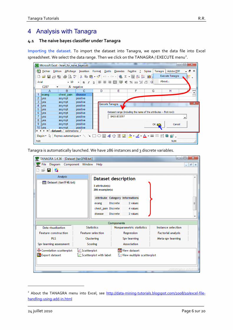
Learning the model. Before the learning process, we must specify the target attribute (DISEASE) and the predictors (EXANG, CHEST_PAIN). We use the DEFINE STATUS component.
We can add the NAIVE BAYES CLASSIFIER component now (SPV LEARNING tab) into the diagram. We click on the VIEW menu to get the results.
Into the upper part of the visualization window, we get the confusion matrix and the error rate computed on the learning sample (resubstitution error rate).

Tanagra Tutorials R.R.
24 juillet 2010 Page 8 sur 20
The main new feature in the version 1.4.36 of Tanagra is in the lower part of the window. “Model description” provides the parameters of the classification functions. The deployment of the model outside the Tanagra context (e.g. into a spreadsheet) is greatly facilitated.
We obtain the parameters computed manually previously (section 2.3.4). Because we deal with a binary problem, we can extract the decision function.
positive negativeexang = yes 0.623189 -2.104134 2.7273chest_pain = asympt 2.797281 1.609438 1.1878chest_pain = atyp_angina 0.587787 2.484907 -1.8971chest_pain = non_anginal 0.875469 1.658228 -0.7828constant -5.134215 -3.714849 -1.4194
Classification functions DecisionfunctionDescriptors
Note: As optional in Tanagra, we can get the details of cross tabulations used for the computation of the conditional probabilities.
4.2 About the others linear classifiers
The methods analyzed in this section can provide a linear classification function. Our aim is to compare the parameters (coefficients) of the models.
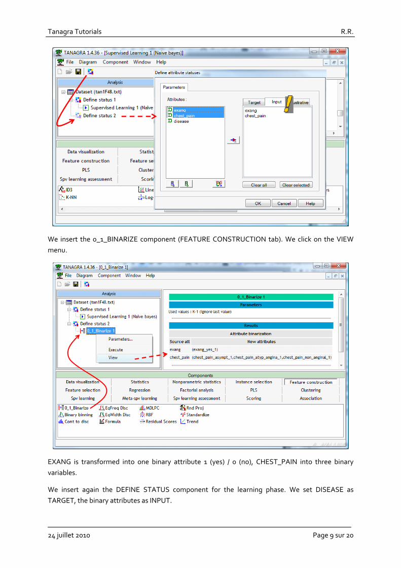
We must explicitly recode the discrete predictors before. We add the DEFINE STATUS component at the root of the diagram. We set EXANG and CHEST_PAIN as INPUT.
Tanagra Tutorials R.R.
24 juillet 2010 Page 9 sur 20
We insert the 0_1_BINARIZE component (FEATURE CONSTRUCTION tab). We click on the VIEW menu.
EXANG is transformed into one binary attribute 1 (yes) / 0 (no), CHEST_PAIN into three binary variables.
We insert again the DEFINE STATUS component for the learning phase. We set DISEASE as TARGET, the binary attributes as INPUT.
Tanagra Tutorials R.R.
24 juillet 2010 Page 10 sur 20
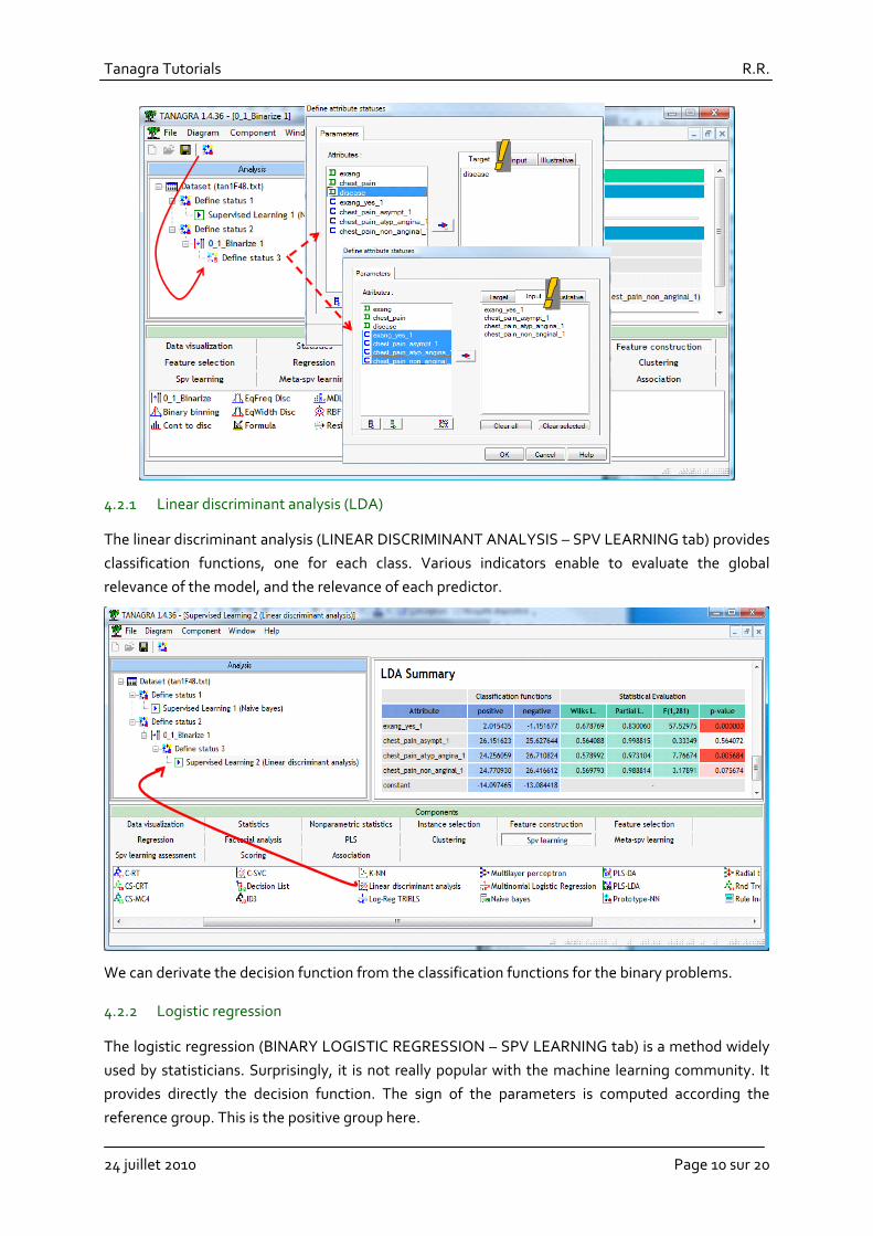
4.2.1 Linear discriminant analysis (LDA)
The linear discriminant analysis (LINEAR DISCRIMINANT ANALYSIS – SPV LEARNING tab) provides classification functions, one for each class. Various indicators enable to evaluate the global relevance of the model, and the relevance of each predictor.
We can derivate the decision function from the classification functions for the binary problems.
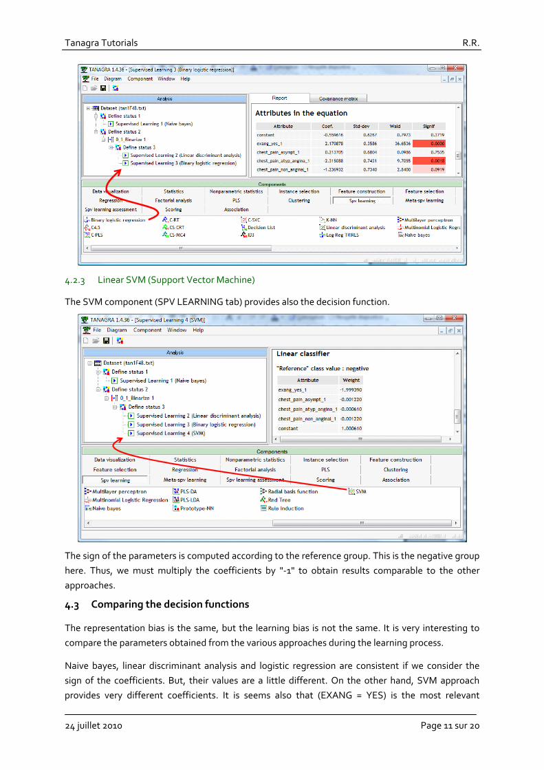
4.2.2 Logistic regression
The logistic regression (BINARY LOGISTIC REGRESSION – SPV LEARNING tab) is a method widely used by statisticians. Surprisingly, it is not really popular with the machine learning community. It provides directly the decision function. The sign of the parameters is computed according the reference group. This is the positive group here.
Tanagra Tutorials R.R.
24 juillet 2010 Page 11 sur 20
4.2.3 Linear SVM (Support Vector Machine)
The SVM component (SPV LEARNING tab) provides also the decision function.
The sign of the parameters is computed according to the reference group. This is the negative group here. Thus, we must multiply the coefficients by "‐1" to obtain results comparable to the other approaches.
4.3 Comparing the decision functions
The representation bias is the same, but the learning bias is not the same. It is very interesting to compare the parameters obtained from the various approaches during the learning process.
Naive bayes, linear discriminant analysis and logistic regression are consistent if we consider the sign of the coefficients. But, their values are a little different. On the other hand, SVM approach provides very different coefficients. It is seems also that (EXANG = YES) is the most relevant

Tanagra Tutorials R.R.
24 juillet 2010 Page 12 sur 20
predictor according to the absolute value of the coefficient. This is rather coherent with the results of the other approaches.
Descriptors Naive Bayes LDA Logistic Reg. Linear SVMexang = yes 2.7273 3.1671 2.1709 1.9994chest_pain = asympt 1.1878 0.5240 0.2137 0.0012chest_pain = atyp_angina -1.8971 -2.4548 -2.3151 0.0006chest_pain = non_anginal -0.7828 -1.6457 -1.2369 0.0012constant -1.4194 -1.0130 -0.5596 -1.0006
About the generalization error rate, on a very simple dataset such as we use in this tutorial, there are not a discrepancy. We use a bootstrap to estimate the error rate (http://data‐mining‐tutorials.blogspot.com/2009/07/resampling‐methods‐for‐error‐estimation.html). We obtain about 20% whatever the method used. These methods often present similar performance on real datasets, except for very specific configurations (e.g. large number of predictors in comparison of the number instances, etc.).
5 Analysis with the other free tools 5.1 Weka 3.6.0
We use Weka in the EXPLORER mode (http://www.cs.waikato.ac.nz/ml/weka/). We launch the tool, then we load the HEART_FOR_NAIVE_BAYES.ARFF data file (Weka file format).
We activate the CLASSIFY tab. We select the NAÏVE BAYES approach. The training sample is both used for the learning and the testing process. We click on the START button.

Tanagra Tutorials R.R.
24 juillet 2010 Page 13 sur 20
We obtain the same confusion matrix as Tanagra. Into the middle part of the visualization window, Weka provides the cross tabulations used for the computation of the various conditional probabilities. We have no information however about the classification functions.
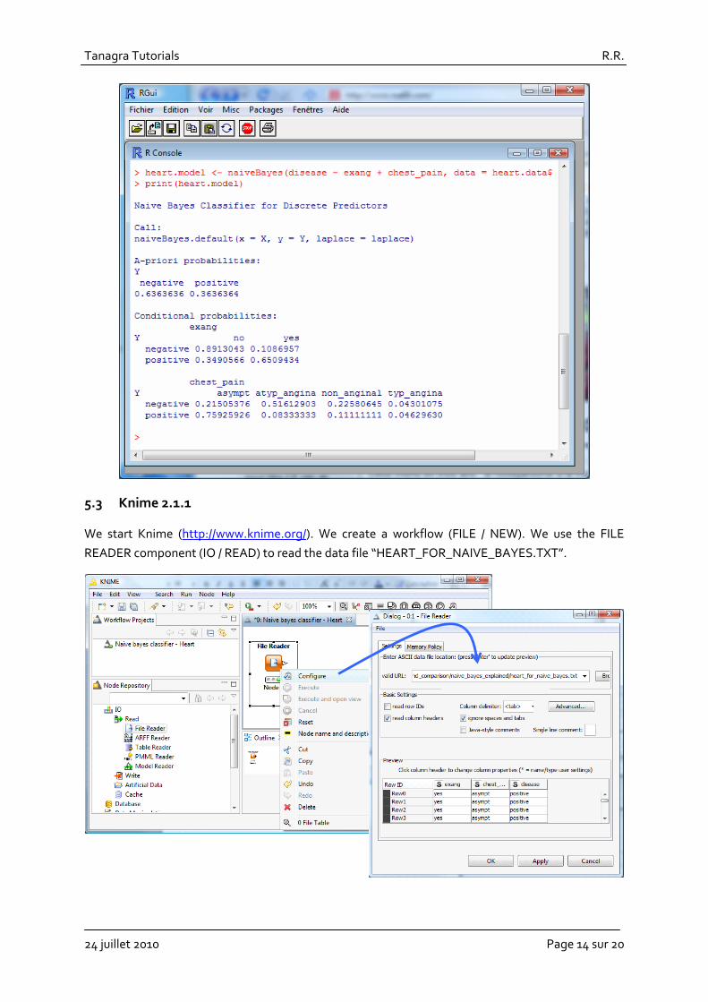
5.2 R 2.9.2
We use the e1071 package (http://cran.r‐project.org/web/packages/e1071/index.html) under R (http://www.r‐project.org/). The source code of our program is the following.
#clear the memory rm (list=ls()) #load the dataset heart.data <- read.table(file="heart_for_naive_bayes.txt",sep="\t",header=T) #build the model library(e1071) heart.model <- naiveBayes(disease ~ exang + chest_pain, data = heart.data, laplace = 1.0) print(heart.model)
The option “laplace = 1” corresponds to “m = 1” for the calculations of the conditional probabilities.
R provides these conditional probabilities in tables. We can compare them to those computed manually previously (section 2.2.1).
Tanagra Tutorials R.R.
24 juillet 2010 Page 14 sur 20
5.3 Knime 2.1.1
We start Knime (http://www.knime.org/). We create a workflow (FILE / NEW). We use the FILE READER component (IO / READ) to read the data file “HEART_FOR_NAIVE_BAYES.TXT”.
Tanagra Tutorials R.R.
24 juillet 2010 Page 15 sur 20
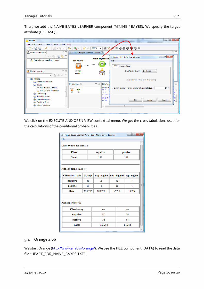
Then, we add the NAÏVE BAYES LEARNER component (MINING / BAYES). We specify the target attribute (DISEASE).
We click on the EXECUTE AND OPEN VIEW contextual menu. We get the cross tabulations used for the calculations of the conditional probabilities.
5.4 Orange 2.0b
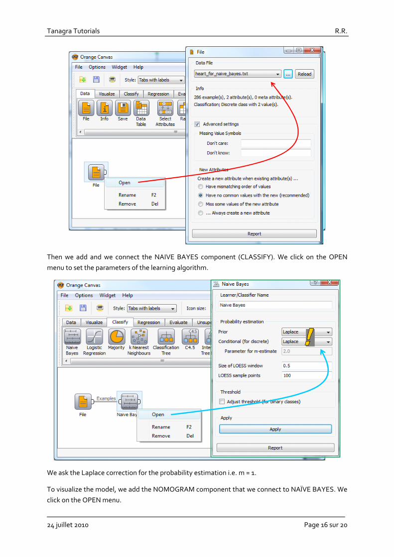
We start Orange (http://www.ailab.si/orange/). We use the FILE component (DATA) to read the data file “HEART_FOR_NAIVE_BAYES.TXT”.
Tanagra Tutorials R.R.
24 juillet 2010 Page 16 sur 20
Then we add and we connect the NAIVE BAYES component (CLASSIFY). We click on the OPEN menu to set the parameters of the learning algorithm.
We ask the Laplace correction for the probability estimation i.e. m = 1.
To visualize the model, we add the NOMOGRAM component that we connect to NAÏVE BAYES. We click on the OPEN menu.
Tanagra Tutorials R.R.
24 juillet 2010 Page 17 sur 20
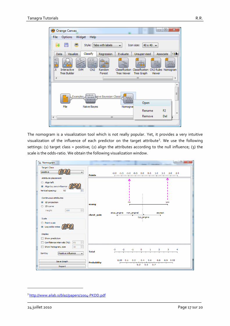
The nomogram is a visualization tool which is not really popular. Yet, it provides a very intuitive visualization of the influence of each predictor on the target attribute3. We use the following settings: (1) target class = positive; (2) align the attributes according to the null influence; (3) the scale is the odds‐ratio. We obtain the following visualization window.
3 http://www.ailab.si/blaz/papers/2004‐PKDD.pdf

Tanagra Tutorials R.R.
24 juillet 2010 Page 18 sur 20
Somehow, the values provided by Orange are very similar to those provided by Tanagra. Let us consider the EXANG predictor. We use the following cross‐tabulation to compute the conditional probabilities.
Nombre de disease exangdisease yes no Totalpositive 68 36 104negative 19 163 182Total 87 199 286
The “odds” is the ratio between the number of positive instances and the number of negative ones.
For the whole sample, it is 57.0182104
= . Within the "EXANG = yes" group, the odds is 58.31968
= . Orange
computes the natural logarithm of the ratio between these odds i.e. 83.157.058.3ln = . This explains the
positioning of this modality into the nomogram. In the same way, for the group "EXANG = no", we
get 95.057.022.0ln −= . Thus, we can conclude that EXANG = YES has a positive influence on the
presence of the DISEASE (DISEASE = yes). If we want a “left alignment”, Orange computes the logarithm of the ratio between the odds of the (EXANG = YES) and (EXANG = NO) groups i.e.
79.222.058.3ln = . This value is very similar (the nomogram does not use the Laplace estimate) to the
coefficient of EXANG = YES into the decision function provided by Tanagra.
5.5 Rapidminer 4.6.0
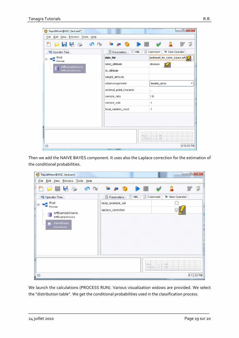
We launch RapidMiner (http://rapid‐i.com/content/view/181/190/). We create a new project by clicking on the FILE / NEW menu. We insert the ARFF EXAMPLE SOURCE component with the following settings.
Tanagra Tutorials R.R.
24 juillet 2010 Page 19 sur 20
Then we add the NAIVE BAYES component. It uses also the Laplace correction for the estimation of the conditional probabilities.
We launch the calculations (PROCESS RUN). Various visualization widows are provided. We select the “distribution table”. We get the conditional probabilities used in the classification process.

Tanagra Tutorials R.R.
24 juillet 2010 Page 20 sur 20
6 Conclusion We highlight into this tutorial an original visualization of the naive bayes classifier when we deal with discrete predictors. The main advantage of this representation is that we can easily deploy the classifier. It is especially interesting in a business process context.
About the continuous predictors, we incorporate a naive bayes classifier intended to the continuous predictors in a future version of Tanagra. We will see also that we can obtain a classifier which is a linear combination of the predictive variables (or the squares of the variables according to the assumptions of homoscedasticity or heteroscedasticity). The deployment of the model is also easy for the case of continuous predictors.
Finally, the naive bayes approach becomes particularly interesting when we combine it with a feature selection system. We will describe it in a future tutorial. Thus, we consider only the relevant and not redundant variables for construction of the final model. The interpretation of the results is easier in this context. Moreover, the classifier is more reliable according to the Occam's Razor principle.
![Una Generalización del Clasificador Naive Bayes para Usarse … · Augmented Naive Bayes (TAN) [6]; Super Parent TAN [7,8]; Improved Naive Bayes (INB) [9]; Weighted NB [10-15]; Taheri](https://img.pdfslide.tips/doc/110x75/5bdd2d7c09d3f2f6568c43de/una-generalizacion-del-clasificador-naive-bayes-para-usarse-augmented-naive.jpg)