Embed Size (px)
Citation preview

- Bogotá - Colombia - Bogotá - Colombia - Bogotá - Colombia - Bogotá - Colombia - Bogotá - Colombia - Bogotá - Colombia - Bogotá - Colombia - Bogotá - Colombia - Bogotá -
The Demographic Transition inColombia: Theory and Evidence Por: Daniel Mejía, María Teresa Ramírez y Jorge Tamayo
No. 5382008

The Demographic Transition in Colombia:
Theory and Evidence*∗
Daniel Mejía† Maria Teresa Ramirez‡ Jorge Tamayo§
Abstract
The demographic transition from high to low mortality and fertility rates was one
of the most important structural changes during the twentieth century in most Latin
American economies. This paper uses a symple economic framework based on Galor
and Weil (2000) for understanding the main forces behind this structural transition;
namely, increases in the returns to human capital accumulation driven by continuous
advances in productivity led families to reduce the number of offspring and increase
the level of investment in their education. As a result, the economy transits from
a stage of stagnation subject to Malthusian forces to a stage of sustained economic
growth, where increases in productivity lead to improvements in living standards. We
use available data for Colombia between 1905 and 2005 to test the main predictions
of the model with time series analysis, finding empirical evidence in their favor.
Keywords: Economic Growth, Demographic Transition, Colombia.
JEL Classification Numbers: C32, J11, N36, O40, O54
∗The authors wish to thank Miguel Urrutia for very helpful comments as well as seminar participants
at Universidad de los Andes.†Assistant professor, Economics Department, Universidad de los Andes, e-mail: [email protected]‡Senior Researcher, Research Unit, Banco de la República, Colombia, e-mail: [email protected]§Research Assistant, Banco de la Republica, e-mail: [email protected]
1

La transición demográfica en Colombia:
Teoría y evidencia.∗
Daniel Mejía† Maria Teresa Ramirez‡ Jorge Tamayo§
Abstract
Uno de los cambios estructurales más importantes ocurridos en los países lati-
noamericanos durante el siglo XX fue la transición demográfica, al pasar de altas a
bajas tasas de mortalidad y fertilidad. Este artículo utiliza una simplificación del
modelo de Galor y Weil (2000) para entender las principales fuerzas detrás de dicha
transición, en la cual incrementos en los retornos a la acumulación de capital humano
derivados de un continuo avance en la productividad lleva a las familias a reducir
el número de hijos e incrementar la inversión en su educación. Como resultado, la
economía se mueve de un estado de estancamiento sujeto a fuerzas Malthusianas a un
estado de crecimiento económico sostenido, donde los incrementos en productividad
llevan a mejoras en los estándares de vida. Para probar sí las principales predicciones
del modelo se cumplen para el caso colombiano se realiza un análisis de series de
tiempo, encontrando evidencia empírica a su favor.
Palabras clave: Crecimiento económico, trancisión demográfica, Colombia.
Clasificación JEL: C32, J11, N36, O40, O54
∗Los autores agradecen los valiosos comentarios de Miguel Urrutia y de los asistentes al Congreso de
Economía Colombiana en la Universidad de los Andes.†Profesor asistente, Facultad de Economia, Universidad de los Andes, e-mail: [email protected]‡Investigador principal, Unidad de Investigaciones, Banco de la República, Colombia, e-mail:
[email protected]§Asistente de investigación, Banco de la República, e-mail: [email protected]
1
1 Introduction
One of the most important structural transformation in most Latin American economies
during the twentieth century was the demographic transition. That is, the transition from
high to low mortality and fertility rates. For instance, mortality rates in Colombia declined
from roughly 23.4 deaths per thousand inhabitants in 1905 to about 13.2 in 1951 and about
5.5 by 2000. Similarly, the fertility rate declined from about 6.4 children for every woman
of reproductive age in 1905 to about 5 during the 1970-75 period to about 2.5 by the end of
the twentieth century.1 In most of the developed economies this transition occurred at the
beginning of the nineteenth century.2 Understanding the economic and demographic forces
behind such structural transformation of the economy has become the focus of a number
of recent studies and one of the most interesting topics in the economic growth literature.
As set out by Galor and Weil (2000) and Galor (2005), the evolution of demographic
and economic variables and their interrelationships through time can be described by a
process that involves three stages: the Malthusian regime, the post-Malthusian period, and
the demographic transition to sustainable growth. As Galor (2005) observed, technological
progress and population growth were insignificant in comparison with modern standards
during the Malthusian period, since the expansion of the agricultural frontier and improve-
ments in technology did not increase per capita income in the long run, but did have an
impact on population size. In the post-Malthusian regime, the process of industrialization
began and technological progress increased, and this caused increases in per capita income.
Nevertheless, the positive effect of per capita income on population growth persisted during
the post-Malthusian regime, and the incremental increase in income generated by techno-
logical progress was in part offset by increases in population. Finally, in the third stage,
during the demographic transition, increases in income were no longer accompanied by an
increase of population, with the result that technical progress and industrialization, and
their interaction with human capital accumulation, led to sustained growth of per capita
income. The increased demand for educated workers as a result of technological progress
and the process of industrialization, increased the returns to human capital accumulation
1See Florez (2000) for an analysis of the sociodemographic transformations in Colombia during the
twentieth century.2See Galor (2005).
2

which, along with lower levels of mortality and higher levels of life expectancy, led to a
reduction in the number of desired offspring (e.g. a decrease in the rate of population
growth), and an increase in investment in their education.
During recent years, the economic growth literature has placed a lot of emphasis in
explaining the endogenous transition in a unified theoretical model that is capable of de-
scribing the process of development and growth in nations through time3. In a seminal
contribution, Galor and Weil (2000) developed a unified endogenous growth model to ex-
plain the evolution of population, technology and output and their interrelationship over
different epochs of human history, with the endogenous reduction in fertility rates playing
a key role in the rise of income per capita above the subsistence level. In this model, the
reduced fertility rate is a response to technological progress, which raises both the demand
for human capital and its rate of return, thus inducing parents to have fewer children
with higher levels of human capital. Other theoretical studies on unified growth models
include Galor and Moav (2002), Hansen and Prescott (2002), Galor and Mountford (2008),
Doepke (2004), Galor (2005), Fernandez-Villaverde (2001), Soares (2005), Cervellati and
Sunde (2007), and Falcao and Soares (2007).
Despite the recent surge in theoretical models aimed at explaining the transition from a
stage of stagnation to a stage of sustained economic growth and the demographic transition,
few studies have empirically estimated the interaction between the evolution of demographic
and economic variables within a unified growth framework. The main problem for such
an empirical analysis is the intrinsically endogenous character of the variables involved in
the explanation. One way to solve this difficulty is to use modern time series econometric
techniques, such as vector autoregressive models (VAR). In this line of work, Nicolini (2007)
uses a multivariate setting to estimate a VAR system for the British economy that includes
annual series for fertility and mortality rates and for real wages from 1541 to 1841. This
allows him to test the Malthusian hypothesis, where an exogenous increase in the real wage
should be followed by an increase in fertility rates (the so-called preventive check) and
a decrease in mortality rates (the so-called positive check). The estimations were made
for the whole sample and for one hundred year intervals (1541-1640, 1641-1740 and 1741-
1840). Impulse response functions (IRF) show that positive checks disappeared before
3See Broadberry (2007) for a review of recent developments in the theory of very long run growth.
3

the middle of the seventeenth century, whereas the preventive check had vanished by the
mid-eighteenth century. In short, Nicolini’s results suggest that the two most important
mechanisms required to restore the Malthusian equilibrium disappeared by the middle of
the eighteenth century in England. Therefore, Nicolini (2007) concluded that England
began to move out of the Malthusian dynamics well before the Industrial Revolution.4
Similarly, Craft and Mills (forthcoming) estimate a VAR system5 that includes crude
birth and death rates and real wages in order to provide quantitative evidence on the
mechanisms of the so-called Malthusian regime in pre-industrial England.6 Unlike Nicolini
(2007), who uses the real wage series of Phelps et al. published in 1956 and the real wages
of workers in London re-estimated by Allen in 2001, Craft and Mills use the latest available
historical data for real wages calculated by Clark in 2005 and covering the period 1263-1913.
Their results share some main stylized facts with Galor and Weil’s (2000) unified growth
theory. For instance, they found that in the Malthusian regime’s real wages showed no
trend up until the onset of the Industrial Revolution. After the Industrial Revolution, wages
take-off. In addition, fast technological progress occurred at the beginning of the nineteenth
century in the so-called post-Malthusian period. Nevertheless, they found that the British
economy had departed far from the Malthusian regime by the middle of the seventeenth
century, earlier than the unified growth model would have predicted. In addition, and in
contrast to this model, the authors did not find any tendency for technological progress to
accelerate as population rose, a key element that helps the economy move away from the
Malthusian trap.7
Other empirical papers, also using time series techniques, have concentrated on the
demographic transition process during the second half of the twentieth century. Hon-
4Previously, Nicolini (2003) included the crude marriage rate in the VAR system, in addition to mor-
tality, fertility and real wages.5To compute the dynamic responses of variables to shocks to one of the variables, Craft and Mills
(forthcoming) use the generalized impulse response functions.6Craft and Mills (forthcoming) perform a series of tests to find a structural break point of the real wage
series. They find a clear break of trend at 1800; before this date real wages were stationary. Therefore,
the empirical analysis focused on the pre-1800 period. However, they estimate VARs, for structural shifts
throughout the period up to 1800 and accumulated 25 years of generalized impulse response functions.7Other papers that conduct quantitative analysis for the demographic transition theory are, for instance
Bar and Leukhina (2008) for England and Greenwood and Seshardi (2002) for the United States. Instead
of using time series techniques, these studies calibrate the models numerically.
4

droyiannis and Papapetrou (2002) analyze the relationship between the fertility and infant
mortality rates, real wages, and real per capita output in Greece during the period 1960-
1996, using vector error correction models, generalized variance decomposition analysis,
and generalized impulse response functions (GIRF). The main result indicates that fertility
changes are endogenous to infant mortality, real wages, and real per capita output. In a
similar way, Climent and Meneu (2004) test the relationship between the same demographic
and economic variables for Spain during the period 1960-2000. Their results suggest the
existence of a long-run relationship between the four variables. In addition, the authors
find that fertility rates and per capita income are clearly endogenous. Specifically, fertility
responds to shocks in income and real wages; real per capita GDP is affected by real wages,
and infant mortality does not cause fertility.
In most of the available literature, empirical research on the co-evolution of demo-
graphic and economic variables has focused on developed economies. To the best of our
knowledge, the only exception is Delajara and Nicolini (2000), who study short-run Malthu-
sian patterns in two Argentine regions with different levels of development (Buenos Aires
and Tucuman) for the period 1914-1970. Using a VAR model, which includes crude birth
rate, crude death rate, crude marriage rate, real wages, and real per capita income, the
authors find significant differences between the regions. In Buenos Aires, Malthusian pre-
ventive checks were common during the period under analysis whereas positive checks were
absent. In contrast, in Tucuman preventive checks were weaker while positive checks were
stronger. The authors conclude that the interactions between demographic and economic
variables in Tucuman resemble that of a pre-industrial economy, while in Buenos Aires
those interactions are similar to those of a modern economy.
This paper presents an economic framework for understanding the main forces behind
the demographic transition in Colombia, and the take-off from a stage of stagnation that
characterized the Colombian economy up until the first half of the twentieth century to a
state of sustained economic growth.
We use annual data for Colombia between 1905 and 2005 to test the main predictions
of the model with time series analysis, finding empirical support in their favor. In the
Malthusian regime a positive shock in per capita income led to increases in the growth
rate of population and has no effect on human capital accumulation, as expected, while in-
creases in real GDP per capita during the modern growth regime do not led to considerable
5

increments in population but, instead, led to increases in human capital accumulation.
The rest of the paper is organized as follows. Section 2 presents the model; section 3
describes some stylized facts of the Colombian demographic transition. Section 4 reports
and discusses the econometric results, and section 5 concludes.
2 The Model
In this section we use Doepke’s (2006) simplified version of Galor and Weil’s (2000) model
to explain the main forces behind the Malthusian and modern growth regimes, and make
special emphasis on the model’s predictions regarding the relationship between the endoge-
nous variables of the model under these different regimes. Namely, the emphasis in this
section will be on the relationship between income, the rate of growth of population, fer-
tility rates, and human capital investment during the different growth regimes. Thus, we
will present the model in the simplest, most intuitive possible way without giving special
emphasis to the details of the underlying dynamical system that governs the evolution over
time of the endogenous variables of the model. In other words, in this section our intention
is not to fully characterize and close the model but, rather, to highlight the crucial forces
and stages behind the demographic transition and the transition from a stage of stagnation
to a stage of sustained economic growth.8 In the empirical exercise we will also account
for other variables that can potentially affect some elements of the model such as mortality
rates. The emphasis of this section on the predictions that are derived from the model
should help us motivate the empirical exercise that will be carried out in section 4.
2.1 Preferences
Individuals derive utility from consumption and a quality-adjusted measure of the number
of offspring they have. More precisely, individuals’ preferences are given by:
u(ct, nt, ht+1) = (1− β) ln ct + β[lnnt + γ lnht+1], with β, γ ∈ (0, 1), (1)
8The reader is refered to Galor and Weil (2000) and Lucas (2002) for a full characterzation of the model
and the evolution of the dynamical system.
6

where c denotes consumption, n the number of offspring, and h the human capital of
each offspring, the latter being a measure of the quality of children.
Furthermore, the time cost of raising a child with no education is φ units of time, and
the time cost of providing the child with e units of education is equal to e. In other words
the model assumes that there is a one-to-one transformation of time invested in children’s
education and the level of education that they achieve.9
Individual’s are endowed with one unit of time that they have to allocate between labor
force participation and child rearing (in both the quantity and quality dimensions, should
they decide to invest in their children’s education). Summing up the costs of child rearing,
the individual’s budget constraint will be given by:
ct = [1− (φt + et)nt]wtht (2)
The budget constraint in equation 2 says that individual’s consumption is equal to
individual’s income, which, in turn, is given by the market wage per unit of human capital,
wt, times the individual’s endowment of human capital, ht, times the amount of time that
the individual has left after investing in child rearing, 1− (φt + et)nt.
Parental time investment in the education of children is transformed into human capital
for their children, ht+1, according to the following human capital production technology:
ht+1 = 1 + μhtet, (3)
where μ > 0 is a parameter that captures the efficiency of parental time investment in
the formation of children’s human capital. Note that the human capital production function
is such that children’s human capital is increasing in their parents’ level of human capital
and on parental time investment in their education. Also, parental education and parental
time investment are complementary in the production of the children’s human capital.
Equation 3 also makes a crucial assumption: if parents do not invest in their children’s
education, children would still have one unit of human capital.10 This assumption reflects
the fact that, even if parents do not invest in their offspring’s education, individuals have
9This is a simplifying assumption that can easily be relaxed. The important point is that children’s
education is a positive and concave function of parental time investment in their offspring’s education.10This assumption guarantees that, under some conditions, the optimal level of investment in children
education is in a corner solution with et = 0.
7

a given endowment of abilities (human capital) that allows them to perform certain basic
tasks.
Finally, another crucial and perhaps realistic assumption of the model (specially for the
early stage of economic development) is that individuals face a subsistence consumption
constraint. Formally:
ct ≥ c, (4)
where c denotes the minimum level of consumption necessary for subsistence.
2.2 Individual’s problem
The problem faced by the representative individual is to choose non-negative values of ct,
nt, and et , in order to solve the following maximization problem:
max{ct,nt,et}
u(ct, nt, ht+1) (5)
subject to : 2, 3, 4,
Two types of solutions emerge from the individual’s optimization problem in equation
5, a corner solution and an interior solution. As we shall see, each of these two possible
solutions characterize the Malthusian epoch and the modern growth regime, respectively.
Explicitly modelling the production side, the determination of wages, and the process
that governs technological progress is beyond the scope of this paper. We will simply
assume that technological progress takes place and, as a result, wages raise over time.
Furthermore, one can think that technological progress is function of the size of population
(as in Kremer, 1993) or a function of the per capital level of education and the size of the
population (as in Galor and Weil, 2000). For the sake of our objective in this section, the
important point to keep in mind is that wages raise over time as a result of technological
progress, which increases the underlying returns to parental time investment in the human
capital of their children. Other factors such as increases in life expectancy or technological
progress might also raise the incentives for parents to invest in the human capital of their
offspring by increasing the parameter μ in equation 3.
8

2.3 The Malthusian epoch
Let us first start with the corner solution of the model. If the income level of the individual,
wtht, is lower than a threshold level that makes the subsistence constraint binding, that is,
if wtht ≤c
1− β, then the solution to the individual’s maximization problem is given by:
c∗t = c = [1− φn∗t ]wtht ⇔ n∗t =1
φ∗t
µ1− c
wtht
¶, and, (6)
e∗t = 0. (7)
Notice that, because wages are increasing over time as a result of technological progress
and the solution says that parents do not invest time and effort in the education of their
children, implies that ht will be equal to 1 (individuals only have the skills to perform
vary basic tasks) and, thus, the subsistence constraint will be binding if the wage rate is
sufficiently low. More precisely, the subsistence constraint is binding for wt ≤ w =c
1− β.
According to the solution in 6, in the early epoch of economic development income is low,
consumption remains at a subsistence level, there is no investment in the quality of children
(e.g. in their education) and the relationship between income, wtht, and population growth
is positive - that is, positive shocks to income increase the number of desired offspring
which in turns dilutes the initial increase in income. Furthermore, during the Malthusian
epoch, there is no relation between income and human capital investment, as in this early
epoch of economic development there is no investment in the quality of children (e.g. in
human capital). The mechanism underlying this solution is purely a Malthusian one. That
is, any increase in income, due to the fact that there is (slow) technological progress, will
translate into a larger population size and not into higher standards of living, as captured
by the income level. Individuals in this early epoch do not invest in human capital and,
thus, there is no relationship between increases in income (due to technological progress)
and increases in the rates of investment in human capital accumulation.
2.4 The modern growth regime
As technological progress continues to take place as a result of increases in the size of the
population, the economy will reach a point where wages are sufficiently high and the sub-
sistence consumption constraint becomes no longer binding. This is a so-called “interior”
9

solution that is fully characterized by the following equations (derived from the first order
conditions associated with the problem in equation 5):
c∗∗t = (1− β)wtht, (8)
n∗∗t =β
φ+ e∗∗t, and,
e∗∗t =1
1− γ
µγφ− 1
μht
¶.
The modern growth regime arises at a point where income is sufficiently high (that is,
when wt >c
1− β) and, as a result, the subsistence consumption constraint is no longer
binding. At this stage of the development process, increases in income, resulting from an
underlying process of technological progress, do translate in to higher standards of living,
higher investment in education, and lower population growth. The solution for nt under
this regime captures the quantity-quality trade-off. That is, the number of children that
parents choose to have is negatively associated with the optimal level of investment in
education that they choose to give to each child.
During this modern epoch of the development process, increases in income no longer
translate into a larger population size and as a result standards of living rise and the econ-
omy transits from a stage of stagnation characterized by the Malthusian forces described
before into a stage of sustained economic growth. Increases in wages (due to the underlying
process of technological progress) increase the returns to human capital accumulation and
parents optimally substitute the quantity of children for greater quality - that is, for more
time investment in their education. As a result, the rate of growth of population decreases
as income increases and, as a result, the economy takes-off from a stage of stagnation to a
stage of sustained economic growth.
3 The Stylized facts of the Colombian demographic
transition
In Colombia, we have identified the two stages: the Malthusian regime and the sustained
economic growth regime. These have characterized the interrelationships among demo-
graphic and economic variables in Colombia as follows:
10

The Malthusian regime
According to the available data, the nineteenth century and the first half of the twentieth
century in Colombia can be characterized as a Malthusian period, with low levels of per
capita income, low economic and population growth, very high mortality and fertility rates
and very low life expectancy and human capital accumulation rates, in the context of a
rural and agrarian economic structure.11 In general, the period is characterized by poor
economic and living conditions.
Colombian economic growth was very slow during the nineteenth century. According
to Kalmanovitz (2008), during the nineteenth century, per capita income grew only at 0.1
percent per year. During the first half of that century per capita income remained stagnant
with almost zero growth, grew at an annual rate of 0.5 percent during the period 1851-86
(explained mainly by an increase in exports) but decreased between 1887 and 1905 because
of civil wars and macroeconomic disequilibria that occurred at the end of the century.12
The country was also very poor. Kalmanovitz (2008) estimates that in 1800 the level of
Colombian per capita income was 69 percent of Mexico’ per capita income and only 39
percent of that of the United States. Fifty years later, the country was even poorer, and
Colombian per capita income was 20 percent of that in the United States; by 1913 it was
only 13 percent. In addition, Urrutia (forthcoming) shows that urban real wages did not
increase during the nineteenth century. In other words, there was no trend of long-run
economic growth in real wages during this period in Colombia, which suggests that per
capita urban income, reflecting an economy with few changes, did not increase during this
time period.
Regarding population, a recent study by Florez and Romero (forthcoming) shows the
evolution of the basic demographic parameters of the Colombian population during the
nineteenth century. They found that population was stable throughout the century, with
high but decreasing fertility and mortality rates. The annual average rate of growth was
almost constant during the first 70 years of the nineteenth century, approximately 1.6
percent on average. Then the rate of population growth started to increase and reached
11According to the 1870 Colombia census, 54% of the working population was employed in agriculture,
cattle-raising and fishing.12The civil war at the end of the century and the financing of the fiscal deficit with money emission were
translated into a macroeconomic disequilibrium.
11

approximately 1.8 percent by the end of the century. This increment is associated with
improvements in public health, the expansions of the agricultural frontier, and the settle-
ments in the Antioquia and Cauca regions. These rates appear high for a pre-industrial
economy. For instance, during the seventeenth century the average population growth rate
in England was approximately 0.3 percent per year, and during the first half of the eigh-
teenth century about 0.4 percent.13 However, according to the authors, the population
growth rate in Colombia during 1820-70 was smaller than that in Argentina (2.6%) and
Brazil (2%), although higher than that for Peru (1.1%) or Mexico (0.7%).14
Florez and Romero (forthcoming) calculate that mortality and birth rates were almost
constant between 1800 and 1870. However, both rates subsequently started to decline, with
a lager decline in the mortality rates than in the birth rates. In particular, the mortality
rate decreased from 40 deaths per one thousand people during 1800-70 to 29.5 by the
end of the century. The birth rate declined from 56.6 births per thousand to 47.7 in the
same period. At the same time, fertility rates were very high: 8.5 children per woman of
reproductive age at the beginning of the century (1800-25), and 7.4 children in 1898. Such
high rates were essential to preserve population growth, given the observed high mortality
rates.
Given the poor conditions in the standards of living, health, nutrition, and the low levels
of income, the child mortality rate was high, although decreasing through the century.
Florez and Romero (forthcoming) estimate that during the first part of the nineteenth
century, the child mortality rate was 297 deaths of children younger than one year old
per thousand births, but had fallen to 250 by the end of the century. Among the factors
behind the decline in the mortality rate were the improvements in nutrition and sanitary
conditions.15 Life expectancy at birth was also very low in nineteenth-century Colombia.
At the beginning of the century it was 26.5 years on average, and it rose to 31 years by the
end of the century.
In terms of human capital, Colombia was one of the world’s most backward countries
in education during the nineteenth century. The ratio of primary school students to total
13See Madison (2000) and Bar and Leukhina (2008).14Florez and Romero (forthcoming) made this comparison with information on Latin American popula-
tion growth calculated by Coastworth in 1998.15See Florez and Romero (forthcoming) and Meisel and Vega (2007).
12

population was considerably smaller in Colombia than in developed countries, and even less
than the Latin America average (graph 1). For instance, by the mid-nineteenth century in
the United States, the number of primary school students relative to total population was
nearly 20 percent. It was more than 10 percent in Holland and the United Kingdom, nearly
10 percent in France, and more than 5 percent in Spain. In Colombia this indicator never
reached more than 3 percent, and the gap between Colombia and the developed countries
increased throughout the century. In addition, as Ramirez and Salazar (forthcoming) show,
education in Colombia was not only backward in terms of international patterns but also
presented a very slow expansion; the ratio between the number of children enrolled in
primary education and total population barely grew from 1.5 percent in 1837 to 2.6 percent
in 1898. As a result, educational advances in Colombia were marginal during the course
of the nineteenth century. The failure to achieve a mass coverage in primary education
in Colombia during that century was attributable to the absence of a suitable structure
of incentives for its expansion, given the economic, political, and social organization that
prevailed in the country. In short, nineteenth-century Colombia displayed patterns of a
pre-industrial economy that fit the description of the Malthusian phase of development
relatively well.
Graph 1 Here
Per capita income and population started to increase around 1870, although very slowly.
Some demographic indicators also began to improve. However, at the end of the century the
country faced a bloody civil war (the Thousand Days War, 1899-1902), that led to a serious
crisis in the external and financial sectors, and high levels of inflation and public debt. In
addition, infrastructure was dismantled. Therefore, the little progress that Colombia had
achieved during the last decades of the nineteenth century was interrupted by the war, and
the country finished the century with conditions similar to those at the start of the century.
After the war, a policy of economic reconstruction was adopted and a series of laws
were passed to regulate and organize the country’s public administration. The reconstruc-
tion policies included large public investments in public works, promotion of agricultural
exports, especially coffee, and an active industrialization program. The economy began to
grow at low rates at the beginning of the twentieth century, and both population and per
capita income increased (graphs 2 and 3). The average real per capita GDP growth was
2.7 percent per year during 1905-50, and population grew at an annual average rate close
13

to 2.3 percent, explained by a high fertility rate and the decline in the mortality rate that
occurred during the 1920s. Also, the real manufacturing wages index grew during these
years (graph 4).
Graphs 2, 3 and 4 here
The standard of living began to improve with higher income, better nutrition and
sanitation, among other factors.16 The mortality rate showed a sustained decline (graph
5). For instance, the child mortality rate fell from 186.5 deaths per thousand births in 1905
to 125 by the end of the 1940s. Life expectancy at birth also improved, from 39.5 years
in 1905 to 48.8 years in 1950. At the same time, the fertility rate increased, as well as
that for education (graphs 6 and 7). Fertility rates rose from 6.4 children per woman of
childbearing age at the beginning of the twentieth century to almost 6.8 by the end of the
1940s. Although education began to expand, especially at the primary level, the expansion
of primary and secondary education in Colombia during the first half of the twentieth
century was very slow. With reconstruction policies at the beginning of the century, that
included the 1903 Law 39 mandating the organization and regulation of education, the
ratio of students enrolled in primary school to total population increased from 3.5 percent
in 1900 to 4.8 percent in 1908, but over the following years this ratio rose only to about 6.7
percent by 1950, which suggests only moderate progress in education during the first half
of the twentieth century. The little progress achieved in primary enrollment kept the gross
enrollment rate in primary education almost constant between 1938 and 1950, averaging
only 34 percent during these years.17
Graphs 5, 6 and 7 here
The modern growth regime
Since the 1950s, Colombia has experienced rapid and sustained economic growth and
significant transformations in its economic and demographic structure. In particular, the
economic structure has moved from agricultural to industrial, communication and services
activities. In the 1950s, the government started an ambitious program of import substitu-
tions to promote the country’s industrialization, which encouraged a considerable increase
in rural migration to the cities and contributed to the increase of urbanization.18 As a
16See Florez (2000) and Meisel and Vega (2007).17See Ramirez and Tellez (2007).18According to Urrutia and Posada (2007) the rural migration to the cities during the 1950s and 1960s
14

result, the urbanization rate rose from 39 percent in 1951 to 50 percent in 1962 and 75
percent in 2000 (graph 8). The migration from rural to urban areas implied a labor force
movement from low productivity activities such as agriculture to higher productivity areas
like manufacturing and services.19
Graph 8 here
The economic transformations that have occurred since the 1950s increased the demand
for more educated workers and induced investment in human capital.20 These factors,
in conjunction with increased fiscal revenue and favorable economic conditions, allowed
education to take off in Colombia. According to Ramirez and Tellez (2007), from 1950
until the mid-1970s, the education indicators for number of students, teachers, and schools
grew at an unprecedented rate in both primary and secondary education. In fact, during
these years the number of students enrolled in primary and secondary grew at a higher rate
than population. For instance, the average annual rate of growth in primary enrollment
during the 1950s was 7.7 percent, and for the 1960s it was 6.9 percent; secondary enrollment
grew to 12.4 percent and 13 percent for the decades, respectively (graph 7).21
Demographic transformations in Colombia were remarkable during the second half of
the twentieth century. In the 1950s the rate of population growth continued to be high (the
average annual rate of growth was close to 3%) because of the still high fertility rates and
declining mortality rates (graph 5).22 However, by the mid-1960s the fertility rate began
to decrease significantly as a consequence of the decline in the child mortality rate, birth
control planning, and the high opportunity cost for women with a greater participation in
the labor force, among other factors.23 As graphs 7 and 9 show, the decline in fertility
was preceded by an increase in the human capital investment and its rate of returns. This
decline in fertility and a continuing decline in the mortality rate, led to a reduction in
was mainly motivated by the rural-urban wage differential.19See Urrutia and Posada (2007).20According to Echavarria (1999), since the 1930s the industrialization process has brought a substantial
increase in the demand for a skilled labor force since the earlier experience with unskilled labor was
unfruitful.21For details of the evolution of the education in Colombia during the twentieth century, see Ramirez
and Tellez (2007).22Florez (2000) characterized this period as a demographic explosion in Colombia, with average rate of
population growth more than two times higher than that in Europe during the transition.23For details of this transformation, see Florez (2000).
15

the rate of population growth, which was close to 1.8 percent at the end of the twentieth
century (graph 2). In addition, the decline in the mortality rate reflected an increase in life
expectancy at birth, which also had preceded the decline in fertility and which improved
from 49 years in 1950 to 63 years in 1975 and 72 years in 2000.
Graph 9 here
4 Estimations and results
We use modern time series techniques to test the main predictions of the unified growth
model. Because of data availability, our empirical analysis is concentrated on the 1905-2005
period, which includes the end of the Malthusian regime (1905-45) and the demographic
transition period (1955-2005).24
To estimate empirically the interaction between the evolution of the demographic and
economic variables, we use cointegration techniques, vector autoregressions (VAR), and
vector error correction (VEC) models, which serve to identify long-run relationships, in a
multivariate system with non-stationary variables. This allows us to analyze the dynamic
properties of the system by estimating the impulse response functions (IRF) of each vari-
able to shocks in the other variables.25 Also, using these techniques, we can distinguish
between exogenous and endogenous variables, an issue that is important given the complex
interactions among these variables.
In both periods, we estimate two systems. The first one (Model 1) include annual data
for population (P), real per capita gross domestic product (RPGDP) and students enrolled
in secondary education as a proxy for human capital (HC). The second system (Model 2)
includes series of fertility (FR), child mortality (MR) rates, RPGDP and HC26 (Graphs 2,
24We applied recursive cointegration tests to determine structural changes. The results (available upon
request) show that the sample can be divided in such periods.25To check for robustness in the results, we also used Generalized Impulse Response Functions (GIRF),
which constructs an orthogonal set of innovations that does not depend on the VAR ordering. In general,
the results of the GIRFs (available upon request) are very close to the IRFs with Choleski decomposition.
Only in the case of Model 1 in the demographic transition period, the responses of population and human
capital to a shock in real per capita income are slightly lower when using GIRFs.26To check also for robustness in the results, we consider in the systems other variables such as crude
rate of birth and primary enrollment rates. The results of the estimation are basically the same.
16

3, 5 and 7).
4.1 Results for the Malthusian period
Preliminary examination of the stationary properties of the series during this period sug-
gests that all series are integrated of order one, I(1), but their first differences are sta-
tionary I(0), according to the Augmented Dickey Fuller (ADF), Philips and Perron (PP),
and Kwiatkowski et al. (KPSS) tests. Given that the series in levels are not stationary,
we proceed with cointegration tests among the variables, using the Johansen multivariate
methodology for cointegration. The first exercise includes population, real per capita GDP,
and human capital (Model 1). Table 1 presents the cointegration test results, which suggest
a long-run relationship among the variables.27 The trace and λ-max tests indicate again
the presence of a unique cointegration vector.
Table 1 here
Table 2 shows the results of some multivariate tests for checking autocorrelation (LM,
Portmanteau, and L-B tests) and heterocedasticity (White test). The tests indicate that
the system exhibits white noise and no heterocedasticity. In addition, the exclusion, sta-
tionarity, and weak exogeneity tests, presented in Table 3, show that no variables are
excluded from the cointegration vector; all the variables are integrated of order 1 (I(1)),
and only human capital is a weak exogenous variable during the period under analysis. The
character of weak exogeneity of human capital is not surprising during this period, given
its passive role and low levels during the end of the Malthusian regime.
Tables 2 and 3 here
From the VEC model, we estimate the impulse response function (IRF) in which pop-
ulation responds to a positive shock in the real per capita GDP.28 Graph 10 displays these
responses through time (annually).29 As observed, an exogenous positive shock in per
capita income is followed by an increase in population, as predicted by the model during
the Malthusian regime.
27The adequate selected model includes three lags and a deterministic linear trend in the variables levels
(drift model). In all models, the lags were chosen according to the AIC and SIC, considering the most
parsimonious model which had the best behavior in the residuals.28The shock of each variable is fixed as Cholesky one standard innovation of that variable.29The confidence bands in the impulse response functions are obtained by Bootstrapping.
17

Graph 10 here
Then, we estimate a system (Model 2) including series of fertility rate (FR), child
mortality rate (MR), human capital (HC), and real per capita GDP (RPGDP), assuming
that MR is exogenous, as Galor and Weil (2000) do. We find a long-run equilibrium
relationship among FR, HC and RPGDP with a unique cointegration vector (table 4).
Table 4 here
Tables 5 and 6 present the residual multivariate analysis and the multivariate test for
exclusion, stationarity, and weak exogeneity, respectively. The test shows that residuals
are well-behaved and do not present either autocorrelation or heteroscedasticity. Human
capital appears as a weak exogenous variable during this period.
Graphs 11a and 11b depict the response of the fertility rate and human capital to a
shock in real per capita GDP, respectively.30 During this period a positive shock in GDP
produces an increment in the fertility rate, but does not have any effect on human capital,
yet again, as predicted by the model during the Malthusian equilibrium.
Tables 5 and 6 here and Graphs 11a and b here
4.2 Results for the modern growth period
To empirically test the predictions of the model regarding the demographic transition in
Colombia, we perform similar exercises for the 1955-2005 period. We first examine the
stationary properties of the variables, P, RPGDP, HC, FR and MR, using the ADF, the
PP and the KPSS tests, which indicate that all series are integrated of order one, I(1),
while their first differences are I(0). We then proceed to test two models for cointegration
following the Johansen methodology. Table 7 presents the cointegration result for the first
model, which includes population, real per capita GDP, and human capital. The test
suggests that there is not a long-run relationship between the variables.
Table 7 here
Since the series are not cointegrated, we estimate a VAR model in first differences.
Table 8 shows the test for the residual multivariate analysis, which indicates that the
system exhibits white noise and does not present heteroscedasticty problems.
30In the IRFs, we place fertility first, then human capital and per capita GDP.The results are very similar
when we change the ordering of the variables in the VEC.
18

Table 8 here
Unlike results for the Malthusian regime, the IRFs show that an increase in real per
capita GDP does not produce considerable increments in population but causes an impor-
tant increase in human capital (graphs 12a and 12b). These results fit well the character-
istics of a modern growth regime, in which increments in income are not translated into
higher rates of population growth but induce higher rate of human capital accumulation.
Graphs 12a and 12b here
In a second model we include fertility rate, human capital, real per capita GDP, and the
mortality rate.31 The trace and λ-max test indicates the presence of a unique cointegration
vector among fertility, human capital and real per capita GDP, which suggests a long-run
relationship among these variables (table 9). Tables 10 and 11 show the residuals from the
multivariate analysis and the joint tests for exclusion, stationarity, and weak exogeneity.
The test for weak exogeneity suggests that the fertility rate is an exogenous variable, while
human capital is an endogenous variable, as expected during this period.
Tables 9, 10 and 11 here
Finally, graphs 13a and 13b present the estimated impulse-response functions from
the VEC model.32 As observed, an exogenous increase in per capita income produces an
important and positive response in human capital, while the response of fertility to this
shock is negative and very close to zero. These results are in line with the model predictions
for the modern growth regime.
Graphs 13a and 13b here
5 Concluding remarks
While most of the recent contributions in the growth literature have focused on the the-
oretical underpinnings of the transition from a stage of stagnation to a stage of sustained
economic growth, very few studies have tried to bring the unified growth model to the
data to test its main implication. Furthermore, the few studies that have tried to test the
model’s predictions, have done so for now developed economies. By using long time series
31As in the previous case, we assume that mortality rate is exogenous.32In the IRF we also place fertility first, then human capital and per capita GDP. However, it is worth
to mention that the results are very similar when we change the ordering of the variables in the VEC.
19

that cover the whole demographic transition period in Colombia, we test the main predic-
tions of the unified growth model for a developing economy and find empirical support for
the main predictions of Galor and Weil’s unified growth model.
In particular, during the Malthusian regime we find that a positive shock in per capita
income produces increments in the population but not in education, as expected; during
the modern growth regime, increases in real per capita GDP do not produce considerable
increments in population, but do have a positive effect on human capital. These results fit
well the characteristics of modern growth regime, in which increments in income are not
translated into higher rates of population growth but induce higher demand for educated
workers during the industrialization process.
20

References
Bar, Michael and Leukhina, Oksana (2008), “Demographic transition and industrial rev-
olution: Amacroeconomic investigation”, Available at http://www.unc.edu/~oksana/Paper1.pdf
Broadberry, Stephen (2007), "Recent developments in the theory of very long run
growth: A historical appraisal", University of Warwick, Available at:
http://www2.warwick.ac.uk/fac/soc/economics/staff/faculty/broadberry/wp
Cervellati, Matteo and Sunde, Uwe (2007), “Human Capital, Mortality and Fertility:
A Unified theory of the economic and demographic transition”, IZA discussion paper series
# 2905
Climent, Francisco J. and Meneu, Robert (2004), "Demography and Economic Growth
in Spain: A Time Series Analysis" SSRN electronic paper collection, Available at:
SSRN: http://ssrn.com/abstract=482222
Crafts, Nicholas and Mills, Terence, “From Malthus to Solow: How the Malthusian
Economy really evolved?”, Journal of Macroeconomics forthcoming.
Delajara, Marcelo and Nicolini, Esteban (2000), “Short-run Malthusian Patterns and
regional differentiation in Argentina”, working paper DI002/ECO, Universidad Siglo 21,
Cordoba, Argentina.
Doepke, Matthias (2004), “Accounting for fertility decline during the transition to
growth”, Journal of Economic Growth, vol 9, pp. 347-383
Doepke, Matthias (2006), “Growth Takeoffs”, New Palgrave Dictionary of Economics,
2nd Edition.
Echavarria, Juan Jose (1999), Crisis e industrialización: Las lecciones de los treinta,
Tercer Mundo Editores, Banco de la República, Fedesarrollo.
Echavarria, Juan Jose, et al (2007), “El proceso colombiano de desindustrialización”,
Economía Colombiana del siglo XX: un análisis cuantitativo, eds. James Robinson and
Miguel Urrutia, Banco de la República and Fondo de Cultura Económica.
Falcao, Bruno and Soares, Rodrigo (2007), “The Demographic Transition and the Sexual
Division of Labor”, NBER Working Paper No. W12838, Available at SSRN:
http://ssrn.com/abstract=958490
Fernandez-Villaverde, Jesus (2001), “Was Malthus Rigth? Economic Growth and Pop-
ulation Dynamics”, University of Pennsylvania, Available at:
21

http://www.econ.upenn.edu/~jesusfv/pennversion.pdf
Florez, Carmen Elisa (2000), Las transformaciones socio-demográficas en Colombia du-
rante el siglo XX, Banco de la República and Tercer Mundo Editores
Florez, Carmen Elisa and Romero, Olga Lucia, “La demografía de Colombia en el siglo
XIX”, La economía Colombiana en el siglo XIX, eds. Adolfo Meisel and Maria Teresa
Ramirez, Banco de la República and Fondo de Cultura Economica, forthcoming.
Galor, Oded and Weil, David (2000), “Population, Technology, and Growth: From
Malthusian Stagnation to the Demographic Transition and Beyond”, American Economic
Review, vol. 90 # 4, p.p 806-828.
Galor, Oded and Moav, Omer (2002), “Natural selection and the origin of economic
growth”, Quarterly Journal of Economics, vol 117, pp. 1133-1192.
Galor Oded and Mountford, Andrew (2008), “Trading Population for Productivity:
Theory and evidence”, Review of Economic Studies, vol 75 # 4, pp.1143-1179.
Galor, Oded (2005), “From Stagnation to Growth: Unified Growth Theory”, Handbook
of Economic Growth, pp. 171-293.
GRECO (2002) El crecimiento económico colombiano en el siglo XX, Banco de la
República and Fondo de Cultura Económica.
Greenwood, Jeremy and Seshardi, Ananth (2002), “The U.S. Demographic transition”,
American Economic Review (Papers and Proceedings), vol 92 # 2, pp. 153-159
Hansen, Gary and Prescott, Edward (2002), “Malthus to Solow”, American Economic
Review, vol 92, pp. 1205-1217.
Hondroyiannis, George and Papapetrou, Evangelina (2002), “Demographic transition
and economic growth: Empirical evidence from Greece”, Journal of Population Economics,
vol 15, pp. 221-242.
Kalmanovitz, Salomon (2008), “Constituciones y desarrollo económico en la Colombia
del siglo XIX”, Revista de Historia Económica, # 2, año XXVI.
Kremer, Michael (1993), “Population Growth and Technological Change: One Million
B.C. to 1990”, The Quarterly Journal of Economics, vol. 108(3), pages 681-716.
Londoño, Juan Luis (1995), Distribución del ingreso y desarrollo económico: Colombia
en el siglo XX, Tercer Mundo Editores, Banco de la República and Fedesarrollo, Bogotá.
Lucas, Robert (2002), The Industrial Revolution: Past and future. Lectures on Eco-
nomic Growth, ch. 5. Harvard University Press.
22

Nicolini, Esteban (2003), “The identification of the Malthus World using Vector Au-
toregression”, Available at:
http://www2.wiwi.hu-berlin.de/wpol/schumpeter/seminar/pdf/nicolini.pdf
Nicolini, Esteban (2007), “Was Malthus right? A VAR analysis of economic and demo-
graphic interactions in pre-industrial England”, European Review of Economic History, II,
p.p 99-121.
Maddison, Angus, Historical Statistics for the World Economy: 1-2003 AD, available
at:
http://www.ggdc.net/maddison/
Meisel, Adolfo and Vega, Margarita (2007), “La estatura de los Colombianos: Un ensayo
de antropometría histórica: 1905-2003” Economía Colombiana del siglo XX: un análisis
cuantitativo, eds. James Robinson and Miguel Urrutia, Banco de la República and Fondo
de Cultura Económica.
Ramirez, Maria Teresa and Salazar Irene, “Surgimiento de la educación en Colombia,
¿En qué fallamos?”, La economía Colombiana en el siglo XIX, eds. Adolfo Meisel and Maria
Teresa Ramirez, Banco de la República and Fondo de Cultura Economica, forthcoming.
Ramirez, Maria Teresa and Tellez, Juana (2007), “La educación primaria y secundaria
en Colombia en el siglo XX”, Economía Colombiana del siglo XX: un análisis cuantitativo,
eds. James Robinson and Miguel Urrutia, Banco de la República and Fondo de Cultura
Económica.
Soares, Rodrigo (2005), “Mortality reductions, educational attainment, and fertility
choice”, American Economic Review, Vol 95 # 3, p.p 580-601.
Urrutia, Miguel and Posada, Carlos Esteban (2007), “Un siglo de crecimiento económico”,
Economía Colombiana del siglo XX: un análisis cuantitativo, eds. James Robinson and
Miguel Urrutia, Banco de la República and Fondo de Cultura Económica.
Urrutia, Miguel, “Precios y Salarios Urbanos en el siglo XIX”, La economía Colombiana
en el siglo XIX, eds. Adolfo Meisel and Maria Teresa Ramirez, Banco de la República and
Fondo de Cultura Economica, forthcoming.
23

Graph 1
Source: Ramírez M, T and Salazar, I (forthcoming)
Graph 2
Sources: GRECO (2002) and DANE
0.0
5.0
10.0
15.0
20.0
25.0
1830 1837 1843 1846 1850 1860 1870 1875 1881 1886 1890 1896 1900
(percentage of the population)
Students in primary education
France Germany Italy Holland
Sweden Spain United Kingdom United States
Colombia Latin America
0.0
0.5
1.0
1.5
2.0
2.5
3.0
3.5
0
5,000,000
10,000,000
15,000,000
20,000,000
25,000,000
30,000,000
35,000,000
40,000,000
45,000,000
50,000,000
1905
1910
1915
1920
1925
1930
1935
1940
1945
1950
1955
1960
1965
1970
1975
1980
1985
1990
1995
2000
2005
Population in Colombia
Population Population annual rate of growth (%)
24

Graph 3a
Sources: Florez, C. E (2000), GRECO (2002) and DANE
Graph 3b
Sources: GRECO (2002) and DANE
11.000
11.500
12.000
12.500
13.000
13.500
14.000
14.500
15.000
1905
1910
1915
1920
1925
1930
1935
1940
1945
1950
1955
1960
1965
1970
1975
1980
1985
1990
1995
2000
2005
Real per capita GDP in Colombia
-8.0
-6.0
-4.0
-2.0
0.0
2.0
4.0
6.0
8.0
10.0
1906
1911
1916
1921
1926
1931
1936
1941
1946
1951
1956
1961
1966
1971
1976
1981
1986
1991
1996
2001
Annual rate o f growth o f real per capita GDP in Colombia
25

Graph 4a
Source: Echavarria, J. J (2007)
Graph 4b
Source: Echavarria, J. J (2007)
2.00
2.50
3.00
3.50
4.00
4.50
5.0019
24
1928
1932
1936
1940
1944
1948
1952
1956
1960
1964
1968
1972
1976
1980
1984
1988
1992
1996
2000
2004
Log of the real manufacturing unitary wages index (1990=100)
-30.00
-20.00
-10.00
0.00
10.00
20.00
30.00
40.00
50.00
60.00
1925
1929
1933
1937
1941
1945
1949
1953
1957
1961
1965
1969
1973
1977
1981
1985
1989
1993
1997
2001
Rate o f growth o f real manufacture wages
26

Graph 5
Sources: Florez, C. E (2000), GRECO (2002), DANE and author's calculations
Graph 6
Sources: Florez, C. E (2000), GRECO (2002), DANE and author's calculations
0.00
1.00
2.00
3.00
4.00
5.00
6.00
7.00
8.00
0.00
20.00
40.00
60.00
80.00
100.00
120.00
140.00
160.00
180.00
200.0019
05
1910
1915
1920
1925
1930
1935
1940
1945
1950
1955
1960
1965
1970
1975
1980
1985
1990
1995
2000
2005
Mortality and Fertility rates in Colombia
Infant mortality rate (per 1000 of births) Fertility rate (births by woman)
1.00
1.50
2.00
2.50
3.00
3.50
30.00
35.00
40.00
45.00
50.00
55.00
60.00
65.00
70.00
75.00
1905
1910
1915
1920
1925
1930
1935
1940
1945
1950
1955
1960
1965
1970
1975
1980
1985
1990
1995
2000
2005
Li fe expectancy and Population in Colombia
Life expectancy at birth Population annual rate of growth (%)
27

Graph 7
Source: Ramirez, M.T. and Tellez, J. (2007)
Graph 8
Sources: Florez, C. E (2000), World Bank' CD (2006) and author's calculations
0.00
2.00
4.00
6.00
8.00
10.00
12.00
14.00
16.00
18.00
1905
1910
1915
1920
1925
1930
1935
1940
1945
1950
1955
1960
1965
1970
1975
1980
1985
1990
1995
2000
2005
The evolution o f Education in Colombia
Primary enrollment over population (%) Secondary enrollment over population (%)
0.00
10.00
20.00
30.00
40.00
50.00
60.00
70.00
80.00
90.00
1938
1941
1944
1947
1950
1953
1956
1959
1962
1965
1968
1971
1974
1977
1980
1983
1986
1989
1992
1995
1998
2001
2004
Urbanization rate in Colombia
28

Graph 9
Sources: Florez, C. E (2000), Londoño, J. L. (1995) and author's calculations
Graph 10
Impulse response function of population to a shock in real per capita GDP during the Malthusian period: Model 1
Source: Author’s calculations
0.050
0.070
0.090
0.110
0.130
0.150
0.170
0.190
0.210
0.230
0.250
2.00
3.00
4.00
5.00
6.00
7.00
8.0019
38
1941
1944
1947
1950
1953
1956
1959
1962
1965
1968
1971
1974
1977
1980
1983
1986
F ertility rate and Human Capital rate o f return in Colombia
Fertility rate (births by woman) Rate of return of human capital
‐200
0
200
400
600
800
1000
0 1 2 3 4 5 6 7 8 9 10 11 12 13 14 15 16 17 18 19 20
29

Graph 11a
Impulse response function of fertility to a shock in real per capita GDP during the Malthusian period: Model 2
Source: Author’s calculations
Graph 11b
Impulse response function of human capital to a shock in per capita GDP during the Malthusian period: Model 2
Source: Author’s calculations
‐0.05
0
0.05
0.1
0.15
0.2
0.25
0.3
0.35
0.4
0 1 2 3 4 5 6 7 8 9 10 11 12 13 14 15 16 17 18 19 20
-2,000
-1,000
0
1,000
2,000
3,000
4,000
1 2 3 4 5 6 7 8 9 10
30
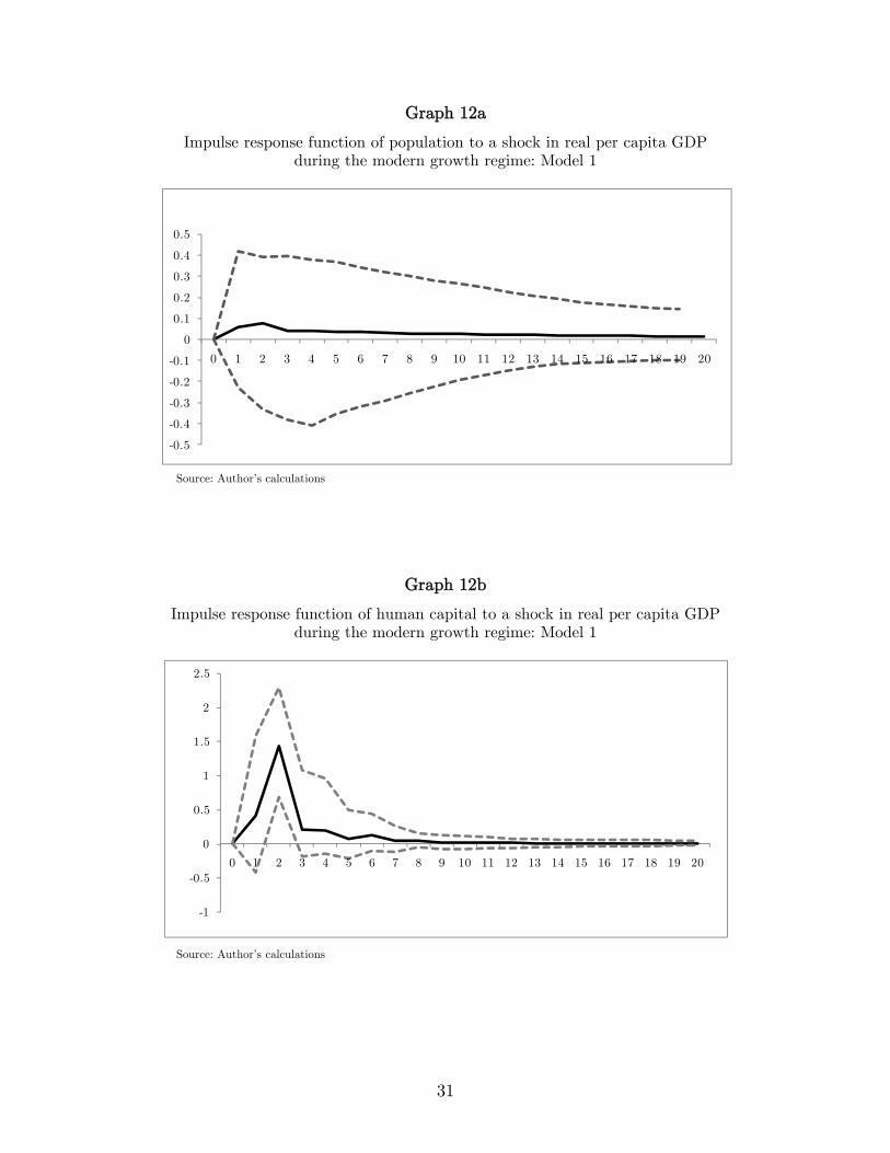
Graph 12a
Impulse response function of population to a shock in real per capita GDP during the modern growth regime: Model 1
Source: Author’s calculations
Graph 12b
Impulse response function of human capital to a shock in real per capita GDP during the modern growth regime: Model 1
Source: Author’s calculations
-0.5
-0.4
-0.3
-0.2
-0.1
0
0.1
0.2
0.3
0.4
0.5
0 1 2 3 4 5 6 7 8 9 10 11 12 13 14 15 16 17 18 19 20
-1
-0.5
0
0.5
1
1.5
2
2.5
0 1 2 3 4 5 6 7 8 9 10 11 12 13 14 15 16 17 18 19 20
31
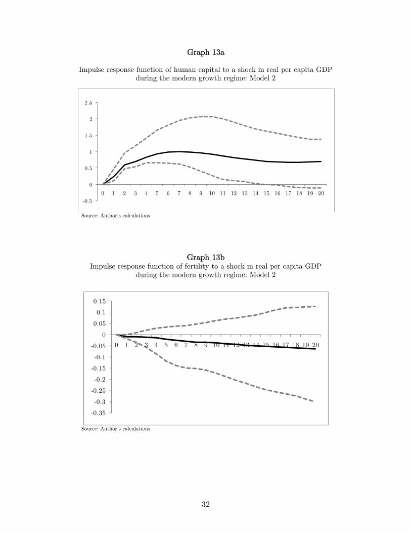
Graph 13a
Impulse response function of human capital to a shock in real per capita GDP during the modern growth regime: Model 2
Source: Author’s calculations
Graph 13b Impulse response function of fertility to a shock in real per capita GDP
during the modern growth regime: Model 2
Source: Author’s calculations
-0.5
0
0.5
1
1.5
2
2.5
0 1 2 3 4 5 6 7 8 9 10 11 12 13 14 15 16 17 18 19 20
-0.35
-0.3
-0.25
-0.2
-0.15
-0.1
-0.05
0
0.05
0.1
0.15
0 1 2 3 4 5 6 7 8 9 10 11 12 13 14 15 16 17 18 19 20
32

Table 1 Cointegration analysis for the Malthusian period: Model 1
System/Model Lag-length
Eigen values λ-max Trace
Statistic Ho:r Critical values
λ-max Trace
{ }ttt HCRPGDPP ,, 0,41 20,14 34,09 0 13,39 26,70 Model: Drift
Lag-Length: 3 0,20 8,33 13,94 1 10,60 13,31 Source: Author’s calculations
Table 2 Residual multivariate analysis for the Malthusian period: Model 1 Heterocedasticity
(p-values) Auto-correlation
(p-values)
No Cross T. Cross T. L-B (12) LM (1) LM (4) Port (1) Port (4)
0,053 0,24 0,15 0,83 0,92 0,056 0,24 Source: Author’s calculations
Table 3 Behavior of the series in the cointegration vector
for the Malthusian Period: Model 1
P HC RPGDP Exclusion Included in
the cointegration
vector
Included in the
cointegration vector
Included in the cointegration
vector Stationarity I(1) I(1) I(1) Weak-exogeneity END EXO END
Source: Author’s calculation
Table 4 Cointegration analysis for the Malthusian period: Model 2
System/Model Lag-length
Eigen values λ-max
Trace Statistic
Ho:r Critical values
λ-max Trace
{ }ttt RPGDPHCFR ,, 0,35 16,85 29,53 0 13,39 26,70 Model: Drift
Lag-Length: 2 0,19 8,28 12,68 1 10,60 13,31 Source: Author’s calculations
33

Table 5 Residual multivariate analysis for the Malthusian period: Model 2 Heterocedasticity
(p-values) Auto-correlation
(p-values)
No Cross T. Cross T. L-B (12) LM (1) LM (4) Port (1) Port (4)
0,05 0,04 0,5 0,97 0,70 0,80 0,84 Source: Author’s calculations
Table 6 Behavior of the series in the cointegration vector
for the Malthusian period: Model 2
FR HC RPGDP Exclusion Included in
the cointegration
vector
Included in the
cointegration vector
Included in the cointegration
vector Stationarity I(1) I(1) I(1) Weak-exogeneity END EXO END
Source: Author’s calculation
Table 7 Cointegration analysis for the modern growth regime: Model 1 System/Model
Lag-length Eigen values
Trace Statistics Ho:r
Critical Value
{ }ttt HCRPGDPP ,, 0,33 26,29
0 29.79
Model: Drift Lag-Length: 3 0,20 5,62
1 15.49
0,002 0,12 2 3.84 Source: Author’s calculations
Table 8 VAR Residual multivariate analysis for
the modern growth regime: Model 1 Heterocedasticity
(p-values) Auto-correlation
(p-values)
No Cross T. Cross T. L-B-1 LM-4 Port (1) Port (4)
0,09 0,34 0,96 0,35 0,59 0,09 Source: Author’s calculations
34

Table 9 Cointegration analysis for the modern growth regime: Model 2
System/Model Lag-length
Eigen values λ-max
Trace Statistics Ho:r
Critical values
λ-max Trace
{ }ttt RPGDPHCFR ,, 0,37 22,50 30,86 0 13,39 26,70 Model: Drift
Lag-Length: 3 0,16 8,36 8,36 1 10,60 13,31 Source: Author’s calculations
Table 10 Residual multivariate analysis for
the modern growth regime: Model 2 Heterocedasticity
(p-values) Auto-correlation
(p-values)
No Cross T. Cross T. L-B LM (1) LM (4) Port (1) Port (4)
0,15 0,10 0,4 0,86 0,56 0,04 0,13 Source: Author’s calculations
Table 11
Behavior of the series in the cointegration vector for the modern growth regime: Model 2
FR HC RPGDP
Exclusion Included in the
cointegration vector
Included in the
cointegration vector
Included in the cointegration
vector Stationarity I(1) I(1) I(1) Weak-exogeneity EXO END END
Source: Author’s calculation
35