2009 年諾貝爾經濟學獎得主奧利佛．威廉森（ Oliver Williamson ）和伊利諾．歐斯壯（ Elinor Ostrom ）都不是大部分人所猜測的諾貝爾經濟學獎得

2009年諾貝爾經濟學獎得主

奧利佛．威廉森（ Oliver Williamson）和伊利諾．歐斯壯（ Elinor Ostrom）都不是大部分人所猜測的諾貝爾經濟學獎得主。這也許是因為他們的研究涉及了經濟、法律和政治科學等領域，處理不同於傳統的經濟問題。

1991年諾貝爾經濟學獎得主羅納德．寇斯（ Ronald Coase）認為，某些情況下的交易，由單一組織內部進行決策，會比交給市場有效率。他的論點對經濟學影響頗深

威廉森則使寇斯的理論更為完整，並明確指出適合內部決策的交易具備哪些特徵。

威廉森指出，與投資決策有關的複雜交易，最適合在企業內部完成。

他認為部分原因在於有些經濟交易太過複雜，根本無法訂立可以處理任何可能情況的合約。

但在後來的研究中，他也指出公司內部處理交易有成本，尤其是濫權。

歐斯壯則將心力放在經濟管理的另一個面向──研究人類社群如何管理共有資源，例如，森林、河流等。

由於共有資源有限，經濟學理論預測理性個體會過度使用該資源。

經濟學家大多認為私有化或國有化是解決問題的答案。

而具有政治科學背景的歐斯壯，在生涯早期花了很多時間，研究社群如何管理等資源。

她發現，團體常會訂立複雜的規則和罰則，確保資源的永續性。這種自助管理成效通常相當良好。

此外，成功的非正式組織都具有某些特徵，而在設計管理共有資源的原則時，「賽局理論」、「重複互動理論」等非常有用。

威廉森創建了經濟學理論的新分支，對企業的研究深入程度無人能比。

歐斯壯以「賽局理論」為分析工具，對人與人間的策略互動進行非常多的實驗，有些還回過頭來影響「賽局理論」。

諾貝爾委員會今年決定（和 98年與 02年一樣），鼓勵社會科學界進行跨領域的研究。

彈性 (elasticity)

彈性的定義

彈性的種類需求彈性供給彈性所得彈性交叉彈性

彈性與支出

彈性與市場干預之效果

彈性

對“反應”的精確衡量 … allows us to analyze supply and demand with gre

ater precision. … is a measure of how much buyers and sellers res

pond to changes in market conditions

衡量數量變動敏感的指標 (price elasticity of demand， income elasticity)

需求的價格彈性Price Elasticity of Demand

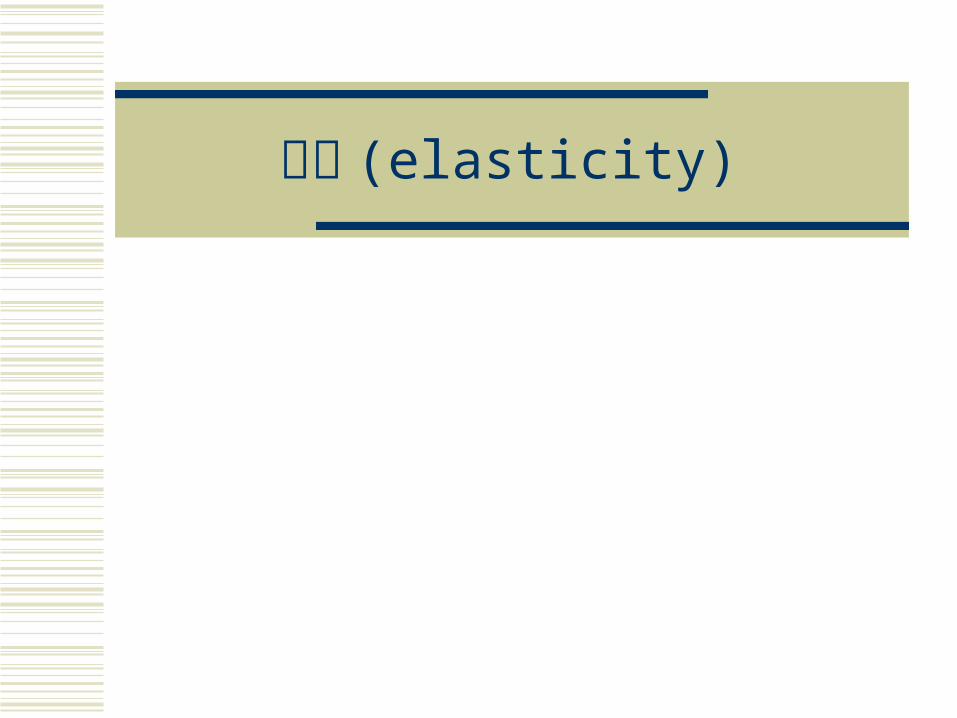
當價格變動百分之一時，需求量改變的百分比

P rice e las tic ity o f d em an d =P ercen tag e ch an g e in q u an tity d em an d ed

P ercen tag e ch an g e in p rice

Price Elasticity of Demand

The price falls to $19.50 and the quantity demanded increases to 11 pizzas an hour.

The price falls by $1 and the quantity demanded increases by 2 pizzas an hour.


The average price is $20 and the average quantity demanded is 10 pizzas an hour.

價格的弧彈性 : 以平均價格與需求量為參考值

通常用於兩點差距較大時


The percentage change in quantity demanded, %Q, is calculated as Q/Qave, which is 2/10 = 1/5.

The percentage change in price, %P, is calculated as P/Pave, which is $1/$20 = 1/20.

The percentage change in quantity demanded, %Q, is calculated as Q/Qave, which is 2/10 = 1/5.

The percentage change in price, %P, is calculated as P/Pave, which is $1/$20 = 1/20.

The price elasticity of demand is (1/5)/(1/20) = 20/5 = 4. 當價格變動百分之一時，需求量改變百分之四

The Midpoint Method: A Better Way to Calculate Percentage

Changes and Elasticities

The midpoint formula is preferable when calculating the price elasticity of demand because it gives the same answer regardless of the direction of the price change.

2 1 2 1

2 1 2 1

( ) /[( ) / 2]Price elasticity of demand =

( ) /[( ) / 2]

Q Q Q Q

P P P P


弧彈性 The Midpoint Meth

od ΔQ/(Q1+Q2) ΔP/(P1+P2)


By using the average price and average quantity, we get the same elasticity value regardless of whether the price rises or falls.

The ratio of two proportionate changes is the same as the ratio of two percentage changes.

The measure is units-free because it is a ratio of two percentage changes and the percentages cancel out.

Changing the units of measurement of price or quantity leave the elasticity value the same.

Computing the Price Elasticity of Demand

Demand is price elastic.

$5

4Demand

Quantity1000 50

3percent 22

percent 67

5.00)/2(4.005.00)(4.00

50)/2(10050)(100

ED

Price


The formula yields a negative value, because price and quantity move in opposite directions. But it is the magnitude, or absolute value, of the measure that reveals how responsive the quantity change has been to a price change.

價、量通常呈反方向變動，因此將彈性取絕對值

彈性 Elasticity (ε)

價格彈性 Price Elasticity

弧彈性 Arc Elasticity =

點彈性 Point Elasticity =

21

21

PPPQQ

Q

Q

P

P

Q

彈性 Elasticity (ε)

點彈性 Point Elasticity = 即為需求線斜率的倒數 ( 取絕對值 )

任一點 p q，需求線愈陡直，斜率愈大，彈性愈小

Q

P

P

Q

P

Q

彈性反映了需求的本質

美國聯邦政府為安全考量強制父母為嬰兒買票，有多少人會改搭汽車 ?


Inelastic and Elastic Demand Demand can be inelastic, unit elastic, or elastic, a

nd can range from zero to infinity. If the quantity demanded doesn’t change when th

e price changes, the price elasticity of demand is zero and the good has a perfectly inelastic demand. 完全無彈性


完全無彈性 a vertical demand cu

rve, elasticity =0 消費者別無選擇


If the percentage change in the quantity demanded equals the percentage change in price, the price elasticity of demand equals 1 and the good has unit elastic demand. 價格彈性 =1，單一彈性(Note that the demand curve is not linear.)雙曲線 XY=k 消費金額固定

The Price Elasticity of DemandElastic Demand: Elasticity Is Greater Than 1

Demand

Quantity

4

1000

Price

$5

50

1. A 22%increasein price . . .

2. . . . leads to a 67% decrease in quantity demanded.


Between the two previous cases, the percentage change in the quantity demanded is smaller than the percentage change in price so that the price elasticity of demand is less than 1 and the good has inelastic demand.

價格彈性小於 1

If the percentage change in the quantity demanded is infinitely large when the price barely changes, the price elasticity of demand is infinite and the good has perfectly elastic demand.

彈性無窮大


Figure 4.3c illustrates the case of perfectly elastic demand—a horizontal demand curve.彈性無窮大消費者有眾多選擇

Total Revenue and the Price Elasticity of Demand

Total revenue is the amount paid by buyers and received by sellers of a good.

Computed as the price of the good times the quantity sold.

QPTR

Figure 2 Total Revenue

Demand

Quantity

Q

P

0

Price

P × Q = $400(revenue)

$4

100

When the price is $4, consumers will demand 100 units, and spend $400 on this good.

Elasticity and Total Revenue along a Linear Demand Curve

With an inelastic demand curve, an increase in price leads to a decrease in quantity that is proportionately smaller. Thus, total revenue increases.

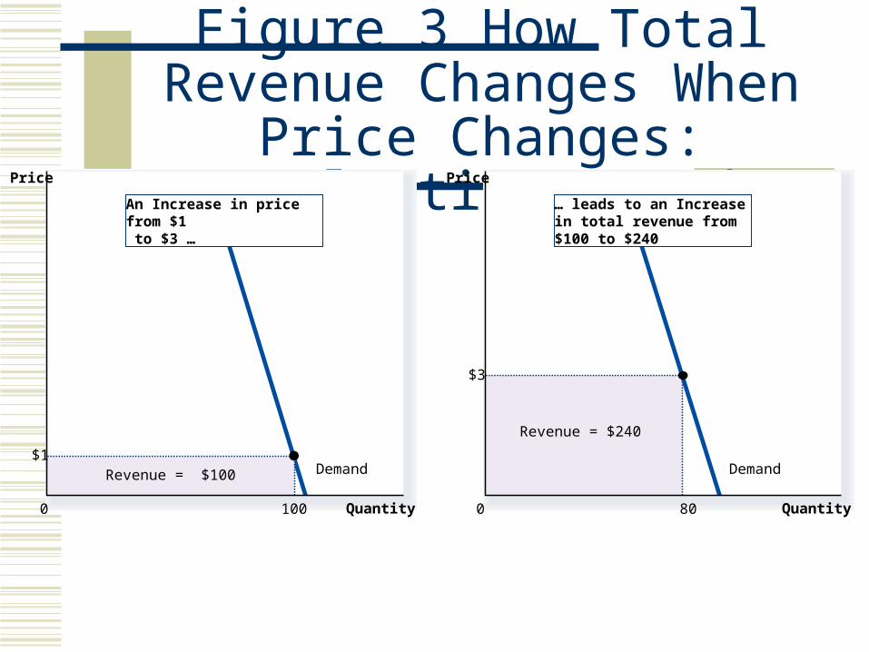
Figure 3 How Total Revenue Changes When Price Changes:

Inelastic Demand

Demand

Quantity0

Price

Revenue = $100

Quantity0

Price

Revenue = $240

Demand$1

100

$3

80

An Increase in price from $1 to $3 …

… leads to an Increase in total revenue from $100 to $240

Elasticity and Total Revenue along a Linear Demand Curve

With an elastic demand curve, an increase in the price leads to a decrease in quantity demanded that is proportionately larger. Thus, total revenue decreases.

Figure 3 How Total Revenue Changes When Price Changes:

Elastic Demand

Demand

Quantity0

Price

Revenue = $200

$4

50

Demand

Quantity0

Price

Revenue = $100

$5

20

An Increase in price from $4 to $5 …

… leads to an decrease in total revenue from $200 to $100

Note that with each price increase, the Law of Demand still holds – an increase in price leads to a decrease in the quantity demanded. It is the change in TR that varies!

Elasticity of a Linear Demand Curve


Elasticity Along a Straight-Line Demand Curve

一條直線需求線上每一點彈性不同

0 2 64 108 12 14

2

1

4

3

5

6

$7

Demand is elastic; demand is responsive to changes in price.

Demand is inelastic; demand is not very responsive to changes in price.

When price increases from $4 to $5, TR declines from $24 to $20.

When price increases from $2 to $3, TR increases from $20 to $24.

Elasticity is > 1 in this range.

Elasticity is < 1 in this range.

Price

Quantity

Figure 4 Elasticity of a Linear Demand Curve


廠商的總收益 ( 消費者的支出 )和消費者的需求彈性有關

彈性 >1 p TR 彈性 =1 p TR 不變彈性 <1 p TR


The total revenue test is a method of estimating the price elasticity of demand by observing the change in total revenue that results from a price change (when all other influences on the quantity sold remain the same).

If a price cut increases total revenue, demand is elastic. If a price cut decreases total revenue, demand is inelastic. If a price cut leaves total revenue unchanged, demand is unit

elastic.


At $12.50, demand is unit elastic and total revenue stops increasing.

As the price falls from $12.50 to zero, demand is inelastic, and total revenue decreases.

Price Elasticity of Demand In part b (shown here),

as the quantity increases from zero to 25, demand is elastic, and total revenue increases.

As the quantity increases from 25 to 50, demand is inelastic, and total revenue decreases.

At 25, demand is unit elastic, and total revenue is at its maximum.

General form

Demand: P=a+ bQ TR=(a+ bQ)Q=aQ+ bQ2

MR= =a+2bQQ

TR

Expenditure and Elasticity

If your demand is elastic, a 1 percent price cut increases the quantity you buy by more than 1 percent and your expenditure on the item increases.

If your demand is inelastic, a 1 percent price cut increases the quantity you buy by less than 1 percent and your expenditure on the item decreases.

If your demand is unit elastic, a 1 percent price cut increases the quantity you buy by 1 percent and your expenditure on the item does not change.


Demand tends to be more elastic: the larger the number of close substitutes. if the good is a luxury/ 佔所得的比重 . the more narrowly defined the market

個別廠商 vs. 產業 . the longer the time period

替代的可能性

The closeness of substitutes +The closer the substitute for a good or service, the more elastic is the demand for it.Necessities, such as food or housing, generally have inelastic demand. 必須品Luxuries, such as exotic vacations, generally have elastic demand. 奢侈品

佔所得的比率

The greater the proportion of income consumers spend on a good, the larger is its elasticity of demand. +

佔所得的比率愈高，價格彈性愈大

距價格改變的時間

The more time consumers have to adjust to a price change, or the longer that a good can be stored without losing its value, the more elastic is the demand for that good. +

距價格改變的時間愈長，價格彈性愈大


Figure 4.6 shows how the elasticity of demand for food varies with the proportion of income spent on food in different countries.

所得彈性 (Income elasticity)

當所得改變百分之一，財貨需求量變動的百分比 The income elasticity of demand measures how

the quantity demanded of a good responds to a change in income, other things being equal.

The formula for calculating the income elasticity of demand is:

Percentage change in quantity demandedPercentage change in income

More Elasticities of Demand

If the income elasticity of demand is greater than 1, demand is income elastic and the good is a luxury good . 奢侈財

Examples include sports cars, furs, and expensive foods If the income elasticity of demand is greater than zero bu

t less than 1, demand is income inelastic and the good is a normal good .正常財 .

Examples include food, fuel, clothing, utilities, and medical services

If the income elasticity of demand is less than zero (negative), the good is an inferior good. 劣等財

More Elasticities of Demand Figure 4.8 shows

estimates of the income elasticity for food in different countries. A higher average income is associated with a lower income elasticity of demand for food.

Cross Elasticity of Demand 交叉彈性

The cross elasticity of demand is a measure of the responsiveness of demand for a good to a change in the price of a substitute 替代財 or a complement互補財 , other things remaining the same.

當一貨價格變動百分之一，其他財貨需求量 ( 供給量 ) 變動的百分比

The formula for calculating the cross elasticity is:Percentage change in quantity demanded

Percentage change in price of substitute or complement

交叉彈性

The cross elasticity of demand for a substitute is positive.

替代財 (substitutes) ：當一物價格下降，導致另一物需求量下降，則兩者互為代替品，　

例：咖啡 vs 茶；糖 vs 代糖

交叉彈性

The cross elasticity of demand for a complement is negative.

互補財 (complements) ：當一物價格下降，導致另一物需求量上升，則兩者互為互補品

例：咖啡 vs 奶精

More Elasticities of Demand

Figure 4.7 shows the increase in the quantity of pizza demanded when the price of a burger (a substitute for pizza) rises.

The figure also shows the decrease in the quantity of pizza demanded when the price of a soft drink (a complement of pizza) rises.

為什麼考慮彈性？

改變價格時，顧客如何反應？（價位該定在何處）

改變價格時，對手如何反應？（改變那一個市場）

改變價格時，自己的收益如何改變？收益改變後，情況可維持多久？

彈性大小與均衡變動

比較靜態分析 (Comparative static analysis) ：探討市場均衡如何因其他條件改變而變動的研究需求彈性小當供給增加 Q* 變動小　 P* 變動大需求彈性大當供給增加 Q* 變動大　 P* 變動小

彈性的差異影響均衡價、量的變化

Price Elasticity of Supply

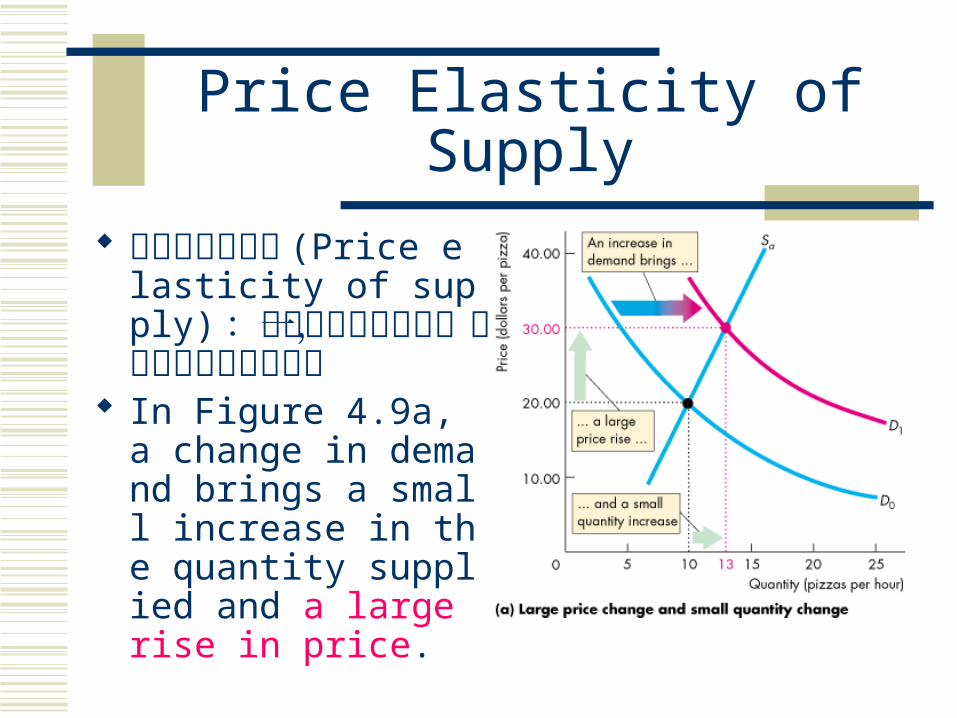
供給的價格彈性 (Price elasticity of supply) ：當價格變動百分之一，供給量變動的百分比

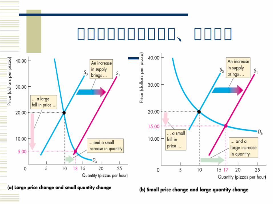
In Figure 4.9a, a change in demand brings a small increase in the quantity supplied and a large rise in price.


In Figure 4.9b, a change in demand brings a large increase in the quantity supplied and a small rise in price.


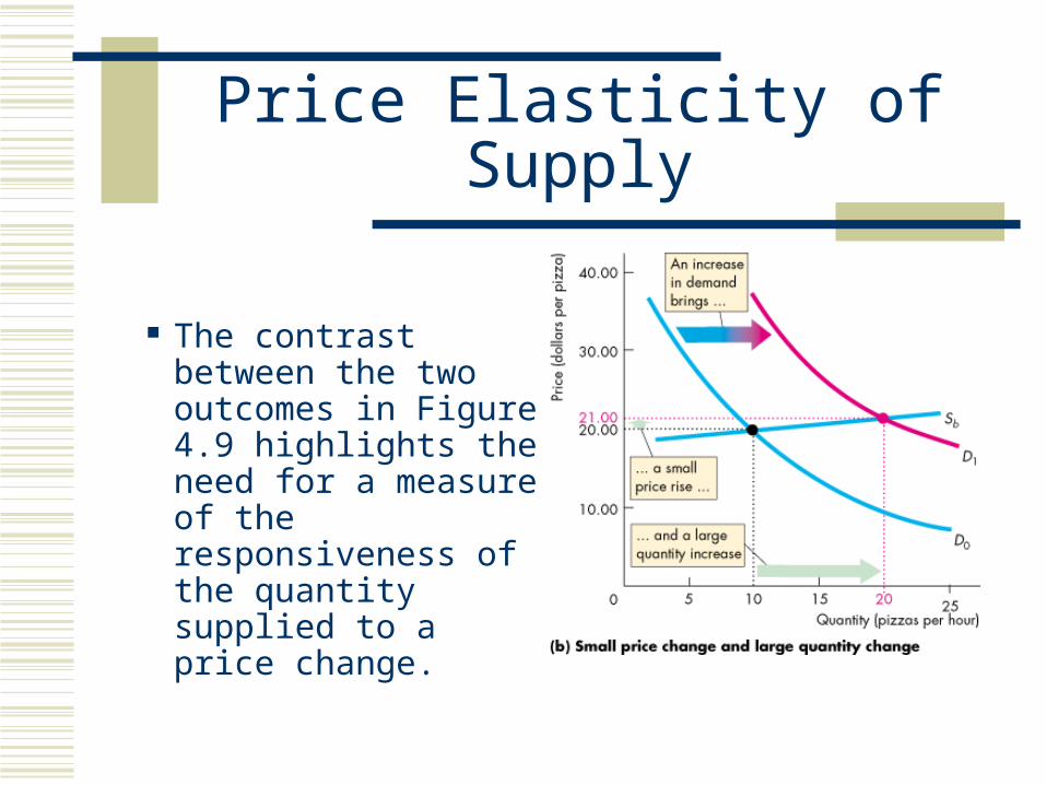
The contrast between the two outcomes in Figure 4.9 highlights the need for a measure of the responsiveness of the quantity supplied to a price change.

供給的價格彈性Elasticity of Supply

The elasticity of supply measures the responsiveness of the quantity supplied to a change in the price of a good when all other influences on selling plans remain the same.

P rice e las tic ity o f su p p ly =

P ercen tag e ch an g e in q u an tity su p p lied

P ercen tag e ch an g e in p rice

Elasticity of Supply

Figure 4.10 on the next slide shows three cases of the elasticity of supply.

Supply is perfectly inelastic if the supply curve is vertical and the elasticity of supply is 0.

Supply is unit elastic if the supply curve is linear and passes through the origin. (Note that slope is irrelevant.)

Supply is perfectly elastic if the supply curve is horizontal and the elasticity of supply is infinite.


S

“Perfectly inelastic” (one extreme)

P

QQ1

P1

P2

Q changes by 0%

0%

10%= 0

Price elasticity

of supply

=% change in Q

% change in P=

P rises by 10%

Sellers’ price sensitivity:

S curve:

Elasticity:

vertical

0

0

S

“Inelastic”

P

QQ1

P1

Q2

P2

Q rises less than 10%

< 10%

10%< 1

Price elasticity

of supply

=% change in Q

% change in P=

P rises by 10%


S curve:

Elasticity:

relatively steep

relatively low

< 1

S

“Unit elastic”

P

QQ1

P1

Q2

P2

Q rises by 10%

10%

10%= 1

Price elasticity

of supply

=% change in Q

% change in P=

P rises by 10%


S curve:

Elasticity:

intermediate slope

intermediate

= 1所有出自原點 ( 即 0,0 ) 的供應曲線，必為單一彈性 .

S

“Elastic”

P

QQ1

P1

Q2

P2

Q rises more than 10%

> 10%

10%> 1

Price elasticity

of supply

=% change in Q

% change in P=

P rises by 10%


S curve:

Elasticity:

relatively flat

relatively high

> 1

S

“Perfectly elastic” (the other extreme)

P

Q

P1

Q1

P changes by 0%

Q changes by any %

any %

0%= infinity

Price elasticity

of supply

=% change in Q

% change in P=

Q2

P2 =Sellers’ price sensitivity:

S curve:

Elasticity:

horizontal

extreme

infinity


The Factors That Influence the Elasticity of Supply The elasticity of supply depends on Resource substitution possibilities + The easier it is to substitute among the resources used to

produce a good or service, the greater is its elasticity of supply.生產要素、生產過程變通、替代的可能

紅茶與綠茶 The time frame for supply decisions The more time that passes after a price change, the greate

r is the elasticity of supply.時間的長短 +


The time frame for supply decisions The more time that passes after a price change,

the greater is the elasticity of supply. Momentary supply is perfectly inelastic. The

quantity supplied immediately following a price change is constant.

Short-run supply is somewhat elastic. Long-run supply is the most elastic.

The supply schedule for chocolate chip cookies is as given in the table above. As the price rises, the elasticity of supply decreases.

P 1.5 P=2.5 3/2 5/4

Price (dollars)

Quantity supplied

1 10

2 30

3 50

4 70

變動緣起

分析對象需求量供給量

商品本身價格需求價格彈性供給價格彈性

其他商品價格需求交叉彈性供給交叉彈性

所得改變需求所得彈性供給所得彈性

彈性大小與均衡變動

比較靜態分析 (Comparative static analysis) ：探討市場均衡如何因其他條件改變而變動的研究需求彈性小當供給增加 Q* 變動小　 P* 變動大需求彈性大當供給增加 Q* 變動大　 P* 變動小　

所以需求或供給彈性大，均衡改變多反應在價格 Q

需求或供給彈性小，均衡改變多反應在價格 P

Can Good News for Farming Be Bad News for Farmers?

Examine whether the supply or demand curve shifts.

Determine the direction of the shift of the curve.

Use the supply-and-demand diagram to see how the market equilibrium changes.

Figure 7 An Increase in Supply in the Market for Wheat

Quantity ofWheat

0

Price ofWheat

3. . . . and a proportionately smallerincrease in quantity sold. As a result,revenue falls from $300 to $220.

Demand

S1 S2

2. . . . leadsto a large fallin price . . .

1. When demand is inelastic,an increase in supply . . .

2

110

$3

100

Compute the Price Elasticity of Demand When There Is a

Change in Supply

ED

1 0 0 11 01 0 0 11 0 2

3 0 0 2 0 03 0 0 2 0 0 2

0 0 9 5

0 40 2 4

( ) /. .

( . . ) /

.

..

Demand is inelastic.

Why Did OPEC Fail to Keep the Price of Oil High?

Supply and Demand can behave differently in the short run and the long run In the short run, both supply and demand for oil

are relatively inelastic But in the long run, both are elastic

Production outside of OPECMore conservation by consumers

Does Drug Interdiction Increase or Decrease Drug-Related

Crime? Drug interdiction impacts sellers rather than

buyers. Demand is unchanged. Equilibrium price rises although quantity falls.

Drug education impacts the buyers rather than sellers. Demand is shifted. Equilibrium price and quantity are lowered.

Price of Drugs

Quantity of Drugs

Price of Drugs

Quantity of Drugs

Drug Interdiction Drug Education

D2

D1

D1

S2

S1S1

The demand for illegal drugs is inelastic.

Interdiction shifts the supply, while education shifts the demand.

In each case, the change in price is the same.

And in the other it goes down.The changes in quantities (and TR) are remarkable. But in one market the price goes up.

Figure 9 Policies to Reduce the Use of Illegal Drugs

實例分析 1以價制量

1960年代煙酒進口公賣，但因需求彈性小，抑制的消費量有限

Q

P

D1

D2

Q2 Q1

實例分析 2穀賤傷農

稻米盛產則價格下降，因需求彈性小，需求數量增加不多，農民總收入減少

Q

P S1

S2

實例分析 3物以稀為貴

需求固定時，供給量減少，則價格上漲

Q

P S2

S1

D

P1

P2

實例分析 4

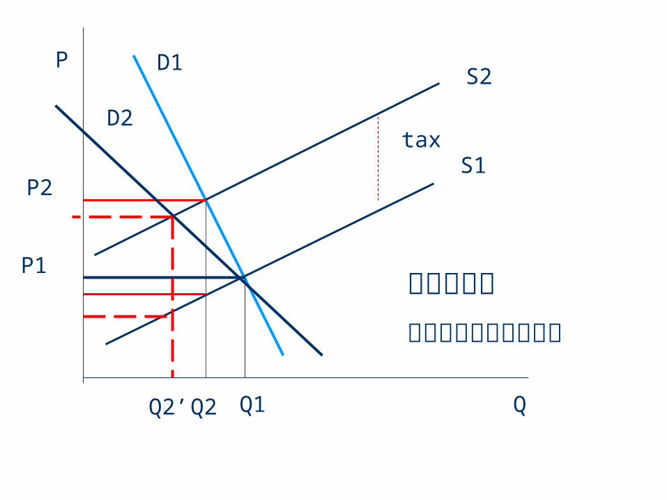
租稅與轉嫁 : 繳稅者未必是真正承擔稅負的人

租稅轉嫁： tax shift，需求彈性愈小，消費者擔愈重，轉嫁愈嚴重

Taxes

The tax revenue takes part of the consumer surplus and producer surplus.

The decreased quantity creates a deadweight loss.

無謂的損失

Q

P

S1

S2

tax

D1

P2

P1

Q2 Q1

需求彈性小消費者承擔的稅負較多

Q

P

S1

S2

tax

D1

P2

P1

Q2 Q1

需求彈性小消費者承擔的稅負較多

D2

Q2’

政府對價量的直接管制

數量管制：供需彈性愈小，供需價格差距愈大黑市運作或其他機制會產生

價格管制

Stabilizing Farm Revenues

An Agricultural Market The supply of farm products is heavily

influenced by natural forces (weather, insects, etc.) beyond the control of farmers.

Consumer demand for farm products is inelastic. These two characteristics combine to make the

market for farm products and farm revenues volatile.


Figure 6.11(a) shows the market for wheat.

Once the crop is planted, supply is perfectly inelastic along the momentary supply curve MS0.

The price is $4 a bushel and farm total revenue is $80 billion.

Stabilizing Farm Revenues A poor harvest decreases supply.

Farmers lose $20 billion of total revenue on the decreased quantity sold.

But they gain $30 billion from the higher price.

Because demand is inelastic, total revenue increases—to $90 billion.


Now a bumper harvest increases supply.

Farmers lose $40 billion of total revenue on the original quantity because the price falls.

They gain only $10 billion from the increased quantity. Because demand is inelastic, total revenue decreases—to $50 billion.


Speculative Markets in Inventories Speculative markets have developed for the inventories o

f those farm products that can be stored over long periods of time. 耐久的農作因此產生投機市場

Inventory holders speculate by: Buying for inventory when the expected future price exc

eeds the current price. Selling from inventory when the current price exceeds th

e expected future price.


Figure 6.12 shows how inventory speculation changes the outcome.

Supply is now perfectly elastic at the price expected by inventory holders—supply curve S.

A poor harvest decreases production but inventories are sold off.


A bumper crop increases production, but some of the extra output goes into inventory.

The price is stabilized at the inventory speculators’ expected price.

投機市場以存貨調節市場價格與交易量


In reality, speculation decreases but does not completely eliminate price fluctuations.

減少價格波動 While speculation does not stabilize farmers’ rev

enues, it changes the effects of bumper harvests and crop failures.

Farmers’ total revenues now increase with bumper crops and decrease with crop failures.

Price elasticity of demand measures how much the quantity demanded responds to changes in the price.

Price elasticity of demand is calculated as the percentage change in quantity demanded divided by the percentage change in price. If a demand curve is elastic, total revenue falls when

the price rises. If it is inelastic, total revenue rises as the price rises.

The income elasticity of demand measures how much the quantity demanded responds to changes in consumers’ income.

The cross-price elasticity of demand measures how much the quantity demanded of one good responds to the price of another good.

The price elasticity of supply measures how much the quantity supplied responds to changes in the price.

In most markets, supply is more elastic in the long run than in the short run.

The price elasticity of supply is calculated as the percentage change in quantity supplied divided by the percentage change in price.

The tools of supply and demand can be applied in many different types of markets.

Documents

2009 年諾貝爾經濟學獎得主 奧利佛．威廉森（ Oliver Williamson ）和 伊利諾．歐斯壯（ Elinor Ostrom ） 都不是大部分人所猜測的諾貝爾經濟學獎得

2009 年諾貝爾經濟學獎得主奧利佛．威廉森（ Oliver Williamson ）和伊利諾．歐斯壯（ Elinor Ostrom ）都不是大部分人所猜測的諾貝爾經濟學獎得