3. Descriptive Statistics Summarization - UMasspeople.umass.edu/~biep540w/pdf/unit03.pdf · BioEpi540W 3. Summarization Page 3 of 24

BioEpi540W 3. Summarization Page 1 of 24

3.Descriptive Statistics

Summarization

Topics 1. The Summation Notation………………………………… 32. Measures of Central Tendency ………….……………… 4

a. The mode ……………………………………….. 7b. The mean ……………………………………….. 8c. The median ……………………………………... 11

3. Measures of Dispersion ………………………………… 13 a. Variance ………………………………………… 14

b. Standard Deviation …………………………….. 15c. Median Absolute Deviation from Median …….. 17d. Standard Deviation v Standard Error …………. 18e. A Feel for Sampling Distributions ……………. 20f. The Coefficient of Variation ………………….. 23g. The Range …………………………………….. 24


Please Quiet Cell Phones and Pagers

Thank you.


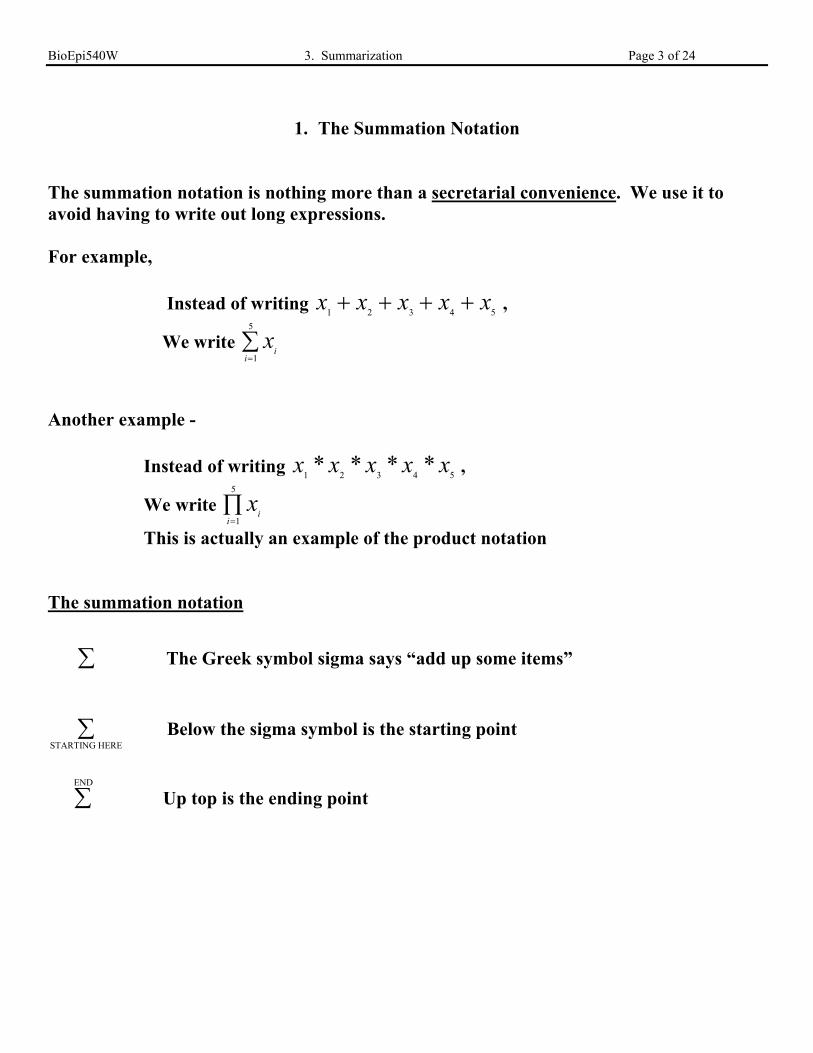
1. The Summation Notation

The summation notation is nothing more than a secretarial convenience. We use it toavoid having to write out long expressions.

For example,

Instead of writing x x x x x1 2 3 4 5+ + + + ,

We write xi

i=∑

1

5

Another example -

Instead of writing x x x x x1 2 3 4 5* * * * ,

We write xi

i=∏

1

5

This is actually an example of the product notation

The summation notation

∑ The Greek symbol sigma says “add up some items”

STARTING HERE∑ Below the sigma symbol is the starting point

END

∑ Up top is the ending point


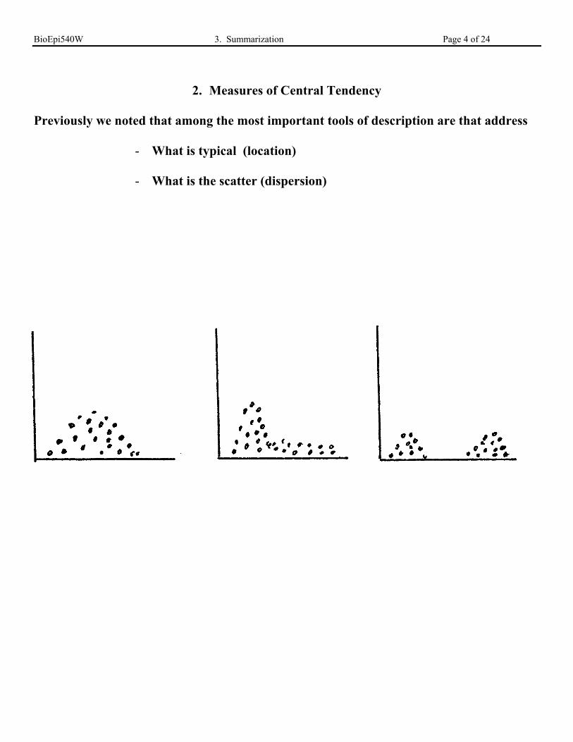
2. Measures of Central Tendency

Previously we noted that among the most important tools of description are that address

- What is typical (location)

- What is the scatter (dispersion)


There are choices for describing location

• Arithmetic average (mean)• Middle most (median)• “Benchmarks” (percentiles)


Mode. The mode is the most frequently occurring value. It is not influenced by extremevalues. Often, it is not a good summary of the majority of the data.

Mean. The mean is the arithmetic average of the values. It is sensitive to extreme values.

Mean = sum of values = Σ (values) sample size n

Median. The median is the middle value when the sample size is odd. For samples ofeven sample size, it is the average of the two middle values. It is not influenced by extremevalues.

We consider each one in a bit more detail …


The Mode

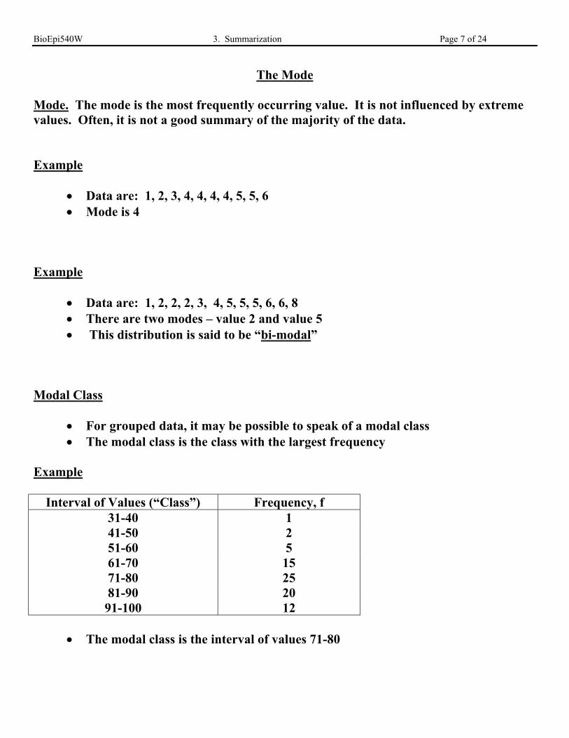
Mode. The mode is the most frequently occurring value. It is not influenced by extremevalues. Often, it is not a good summary of the majority of the data.

Example

• Data are: 1, 2, 3, 4, 4, 4, 4, 5, 5, 6• Mode is 4

Example

• Data are: 1, 2, 2, 2, 3, 4, 5, 5, 5, 6, 6, 8• There are two modes – value 2 and value 5• This distribution is said to be “bi-modal”

Modal Class

• For grouped data, it may be possible to speak of a modal class• The modal class is the class with the largest frequency

Example

Interval of Values (“Class”) Frequency, f31-40 141-50 251-60 561-70 1571-80 2581-90 2091-100 12

• The modal class is the interval of values 71-80


The Mean

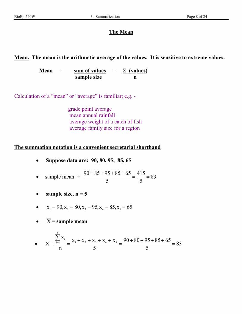
Mean. The mean is the arithmetic average of the values. It is sensitive to extreme values.

Mean = sum of values = Σ (values) sample size n

Calculation of a “mean” or “average” is familiar; e.g. -

grade point average mean annual rainfall average weight of a catch of fish average family size for a region

The summation notation is a convenient secretarial shorthand

• Suppose data are: 90, 80, 95, 85, 65

• sample mean = 90 + 85 + 95 + 85 + 65

5= =

415

583

• sample size, n = 5

• x x x x x1 2 3 4 5= = = = =90 80 95 85 65, , , ,

• X = sample mean

• X =x

n

x x x x x

5

ii=1 1 2 3 4 5

5

90 80 95 85 65

583

∑=

+ + + +=

+ + + +=


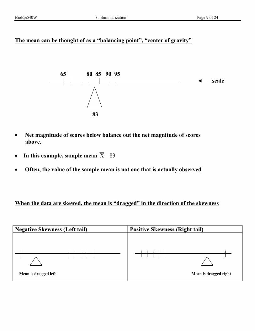
The mean can be thought of as a “balancing point”, “center of gravity”

65 80 85 90 95 scale

83

• Net magnitude of scores below balance out the net magnitude of scores above.

• In this example, sample mean X = 83

• Often, the value of the sample mean is not one that is actually observed

When the data are skewed, the mean is “dragged” in the direction of the skewness

Negative Skewness (Left tail) Positive Skewness (Right tail)

Mean is dragged left Mean is dragged right


The Weighted Mean

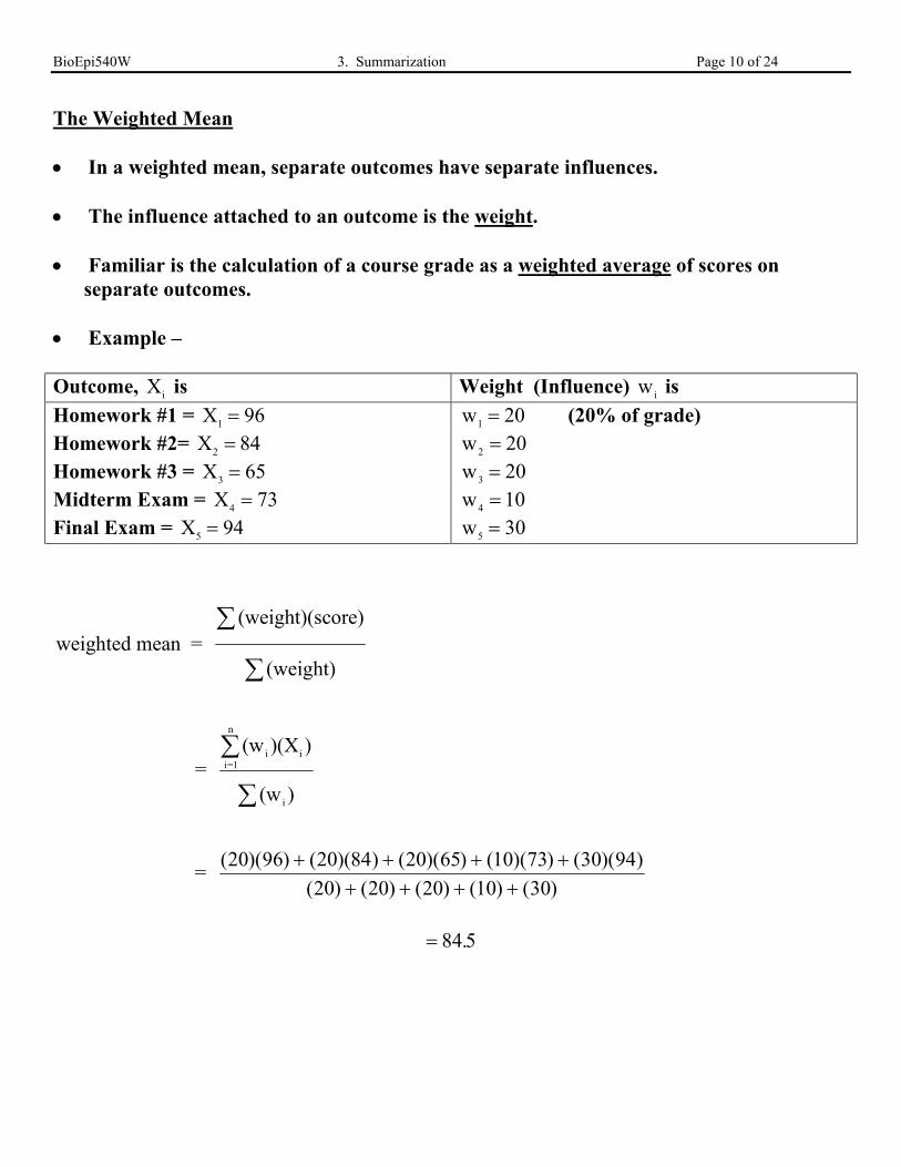
• In a weighted mean, separate outcomes have separate influences.

• The influence attached to an outcome is the weight.

• Familiar is the calculation of a course grade as a weighted average of scores on separate outcomes.

• Example –

Outcome, Xi is Weight (Influence) wi is

Homework #1 = X1 = 96 w1 = 20 (20% of grade)Homework #2= X2 = 84 w2 = 20Homework #3 = X3 = 65 w3 = 20Midterm Exam = X4 = 73 w4 = 10Final Exam = X5 = 94 w5 = 30

weighted mean = (weight)(score)

(weight)

∑

∑

= (w )(X )

(w )

i ii=1

n

i

∑

∑

= ( )( ) ( )(84) ( )( ) ( )( ) ( )( )

( ) ( ) ( ) ( ) ( )

20 96 20 20 65 10 73 30 94

20 20 20 10 30

+ + + ++ + + +

= 84 5.


The Median

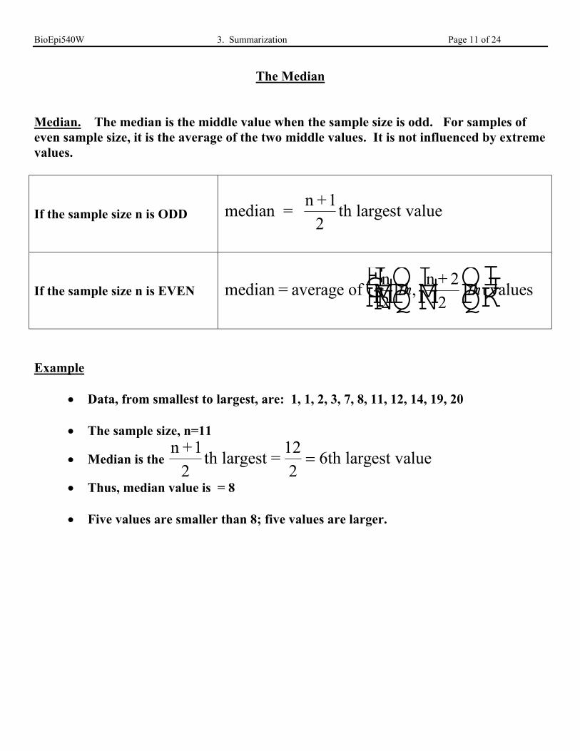
Median. The median is the middle value when the sample size is odd. For samples ofeven sample size, it is the average of the two middle values. It is not influenced by extremevalues.

If the sample size n is ODD median = n +1

2th largest value

If the sample size n is EVEN median = average ofn

2

n + 2

2valuesL

NMOQPLNM

OQP

FHG

IKJth th,

Example

• Data, from smallest to largest, are: 1, 1, 2, 3, 7, 8, 11, 12, 14, 19, 20

• The sample size, n=11

• Median is the n +1

2th largest =

12

26th largest value=

• Thus, median value is = 8

• Five values are smaller than 8; five values are larger.


Example

• Data, from smallest to largest, are: 2, 5, 5, 6, 7, 10, 15, 21, 22, 23, 23, 25

• The sample size, n=12

• Median = average of n

2th largest,

n + 2

2= average of 6th and 7th largest values

• Thus, median value is = average (10, 15) = 12.5

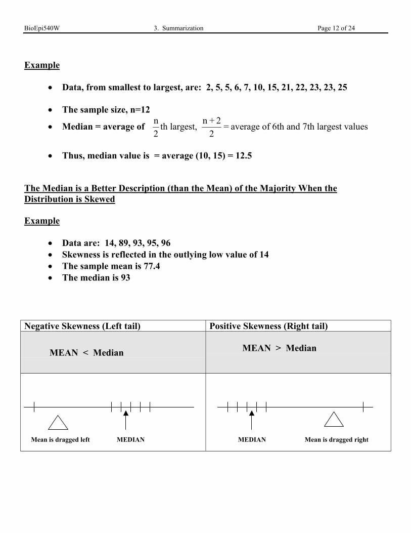
The Median is a Better Description (than the Mean) of the Majority When theDistribution is Skewed

Example

• Data are: 14, 89, 93, 95, 96• Skewness is reflected in the outlying low value of 14• The sample mean is 77.4• The median is 93

Negative Skewness (Left tail) Positive Skewness (Right tail)

MEAN < Median MEAN > Median

Mean is dragged left MEDIAN MEDIAN Mean is dragged right


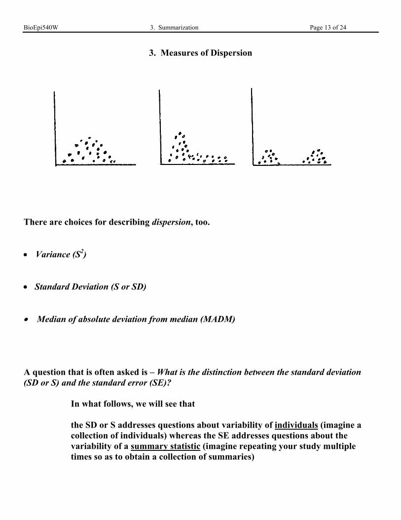
3. Measures of Dispersion

There are choices for describing dispersion, too.

• Variance (S2)

• Standard Deviation (S or SD)

• Median of absolute deviation from median (MADM)

A question that is often asked is – What is the distinction between the standard deviation(SD or S) and the standard error (SE)?

In what follows, we will see that

the SD or S addresses questions about variability of individuals (imagine acollection of individuals) whereas the SE addresses questions about thevariability of a summary statistic (imagine repeating your study multipletimes so as to obtain a collection of summaries)


The Variance

Thinking first about individuals ….

Variance. The variance is a summary measure of the squares of individual departuresfrom the mean.

In a population, the variance of individual values is written σ2.

A sample variance is calculated for a sample of individual values and uses the sample

mean (e.g. X ) rather than the population mean µ. It is written S2 and is almost, but notquite, calculated as the arithmetic average of

(value – mean)2 = (X - X)2

the divisor is (sample size – 1) = (n-1) instead of (sample size).

S2 = sum of (value – sample mean)2

sample size – 1

= ∑ (value – sample mean)2

n – 1

=∑=

(X - X)

n -1

2

i

n

1


The Standard Deviation

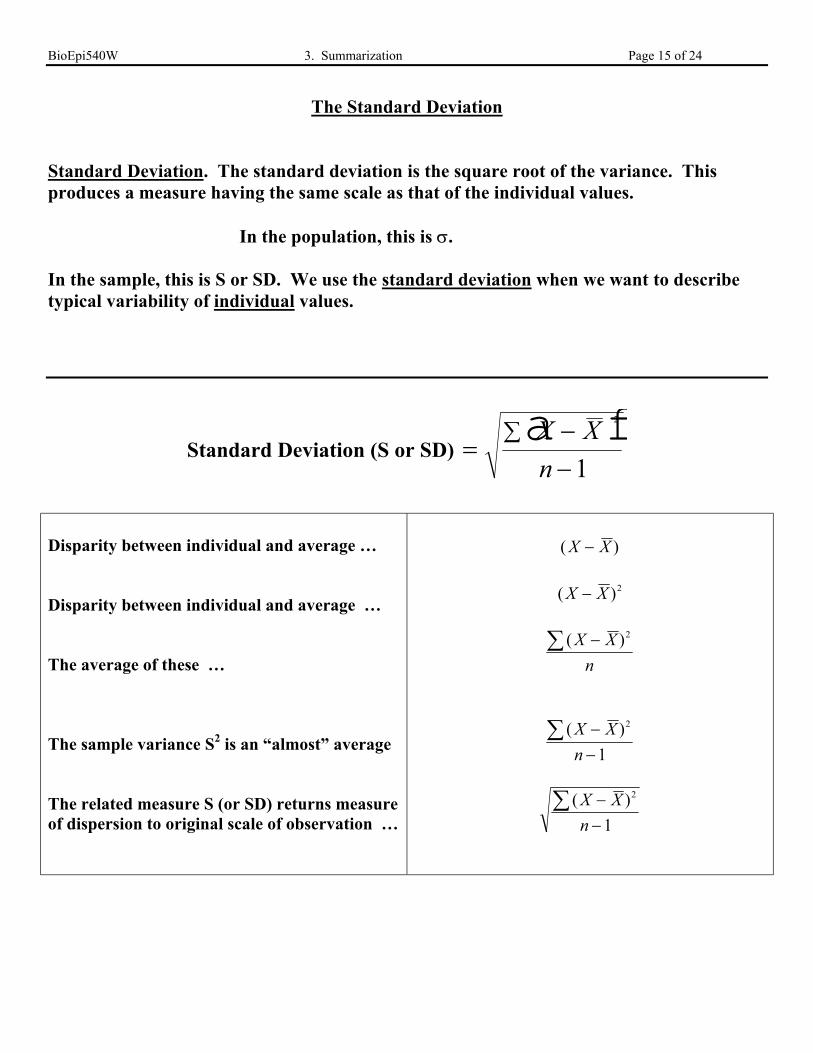
Standard Deviation. The standard deviation is the square root of the variance. Thisproduces a measure having the same scale as that of the individual values.

In the population, this is σ.

In the sample, this is S or SD. We use the standard deviation when we want to describetypical variability of individual values.

Standard Deviation (S or SD) =−−

∑ X X

n

a f21

Disparity between individual and average …

Disparity between individual and average …

The average of these …

The sample variance S2 is an “almost” average

The related measure S (or SD) returns measureof dispersion to original scale of observation …

( )X X−

( )X X− 2

( )X X

n

−∑ 2

( )X X

n

−−

∑ 2

1

( )X X

n

−−

∑ 2

1


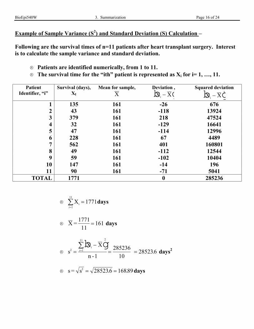
Example of Sample Variance (S2) and Standard Deviation (S) Calculation –

Following are the survival times of n=11 patients after heart transplant surgery. Interestis to calculate the sample variance and standard deviation.

® Patients are identified numerically, from 1 to 11.® The survival time for the “ith” patient is represented as Xi for i= 1, …, 11.

PatientIdentifier, “i”

Survival (days),XI

Mean for sample,

XDeviation ,

X Xi −b gSquared deviation

X Xi −b g21 135 161 -26 6762 43 161 -118 139243 379 161 218 475244 32 161 -129 166415 47 161 -114 129966 228 161 67 44897 562 161 401 1608018 49 161 -112 125449 59 161 -102 10404

10 147 161 -14 19611 90 161 -71 5041

TOTAL 1771 0 285236

® Xi ==∑ 1771

1

11

i

days

® X =1771

11= 161 days

® sX X

n -12

i

=−

= ==∑b gi 1

11 2

285236

10285236. days2

® s = s2 = =285236 168 89. . days


Median Absolute Deviation About the Median (MADM)Still Thinking About Individuals …

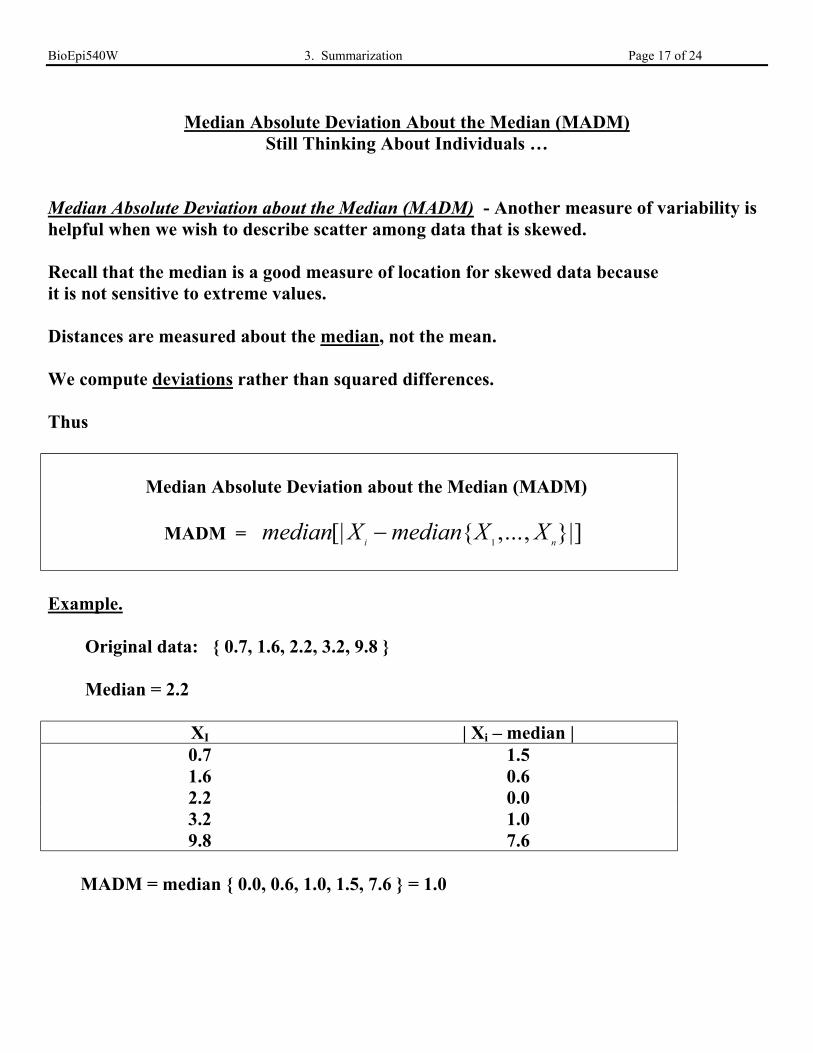
Median Absolute Deviation about the Median (MADM) - Another measure of variability ishelpful when we wish to describe scatter among data that is skewed.

Recall that the median is a good measure of location for skewed data becauseit is not sensitive to extreme values.

Distances are measured about the median, not the mean.

We compute deviations rather than squared differences.

Thus

Median Absolute Deviation about the Median (MADM)

MADM = median X median X Xi n

[| { ,..., }|]−1

Example.

Original data: { 0.7, 1.6, 2.2, 3.2, 9.8 }

Median = 2.2

XI | Xi – median |0.7 1.51.6 0.62.2 0.03.2 1.09.8 7.6

MADM = median { 0.0, 0.6, 1.0, 1.5, 7.6 } = 1.0


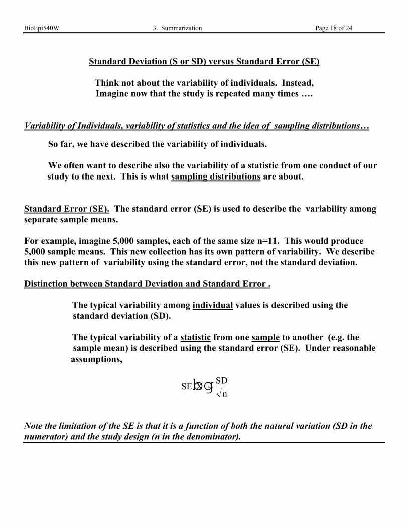
Standard Deviation (S or SD) versus Standard Error (SE)

Think not about the variability of individuals. Instead,Imagine now that the study is repeated many times ….

Variability of Individuals, variability of statistics and the idea of sampling distributions…

So far, we have described the variability of individuals.

We often want to describe also the variability of a statistic from one conduct of our study to the next. This is what sampling distributions are about.

Standard Error (SE). The standard error (SE) is used to describe the variability amongseparate sample means.

For example, imagine 5,000 samples, each of the same size n=11. This would produce5,000 sample means. This new collection has its own pattern of variability. We describethis new pattern of variability using the standard error, not the standard deviation.

Distinction between Standard Deviation and Standard Error .

The typical variability among individual values is described using the standard deviation (SD).

The typical variability of a statistic from one sample to another (e.g. the sample mean) is described using the standard error (SE). Under reasonable assumptions,

SE XSD

nbg=

Note the limitation of the SE is that it is a function of both the natural variation (SD in thenumerator) and the study design (n in the denominator).


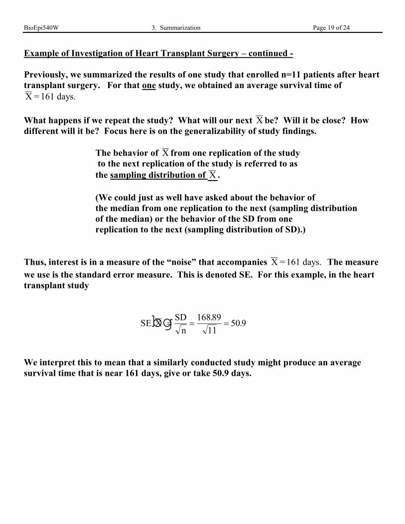
Example of Investigation of Heart Transplant Surgery – continued -

Previously, we summarized the results of one study that enrolled n=11 patients after hearttransplant surgery. For that one study, we obtained an average survival time ofX = 161 days.

What happens if we repeat the study? What will our next X be? Will it be close? Howdifferent will it be? Focus here is on the generalizability of study findings.

The behavior of X from one replication of the study to the next replication of the study is referred to asthe sampling distribution of X .

(We could just as well have asked about the behavior ofthe median from one replication to the next (sampling distributionof the median) or the behavior of the SD from onereplication to the next (sampling distribution of SD).)

Thus, interest is in a measure of the “noise” that accompanies X = 161 days. The measurewe use is the standard error measure. This is denoted SE. For this example, in the hearttransplant study

SE XSD

nbg= = =

168 89

1150 9

..

We interpret this to mean that a similarly conducted study might produce an averagesurvival time that is near 161 days, give or take 50.9 days.


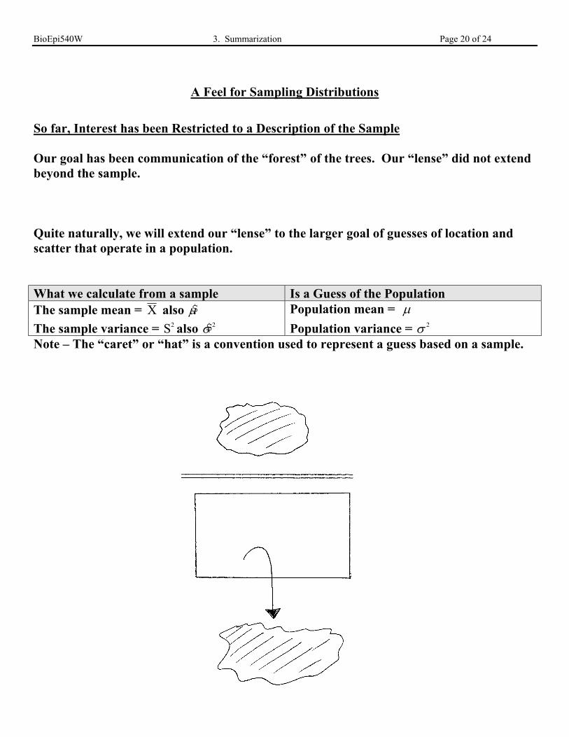
A Feel for Sampling Distributions

So far, Interest has been Restricted to a Description of the Sample

Our goal has been communication of the “forest” of the trees. Our “lense” did not extendbeyond the sample.

Quite naturally, we will extend our “lense” to the larger goal of guesses of location andscatter that operate in a population.

What we calculate from a sample Is a Guess of the PopulationThe sample mean = X also $µ Population mean = µThe sample variance = S2 also $σ 2 Population variance = σ 2

Note – The “caret” or “hat” is a convention used to represent a guess based on a sample.


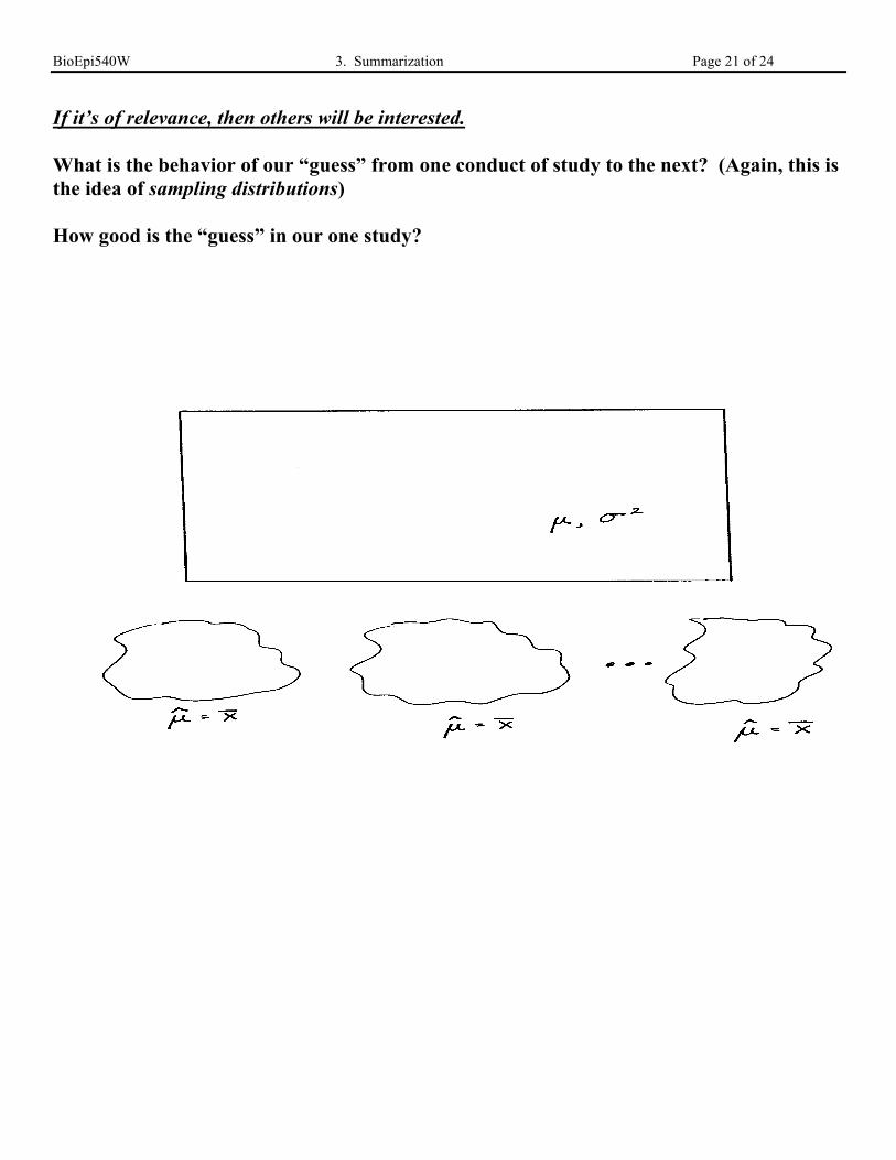
If it’s of relevance, then others will be interested.

What is the behavior of our “guess” from one conduct of study to the next? (Again, this isthe idea of sampling distributions)

How good is the “guess” in our one study?


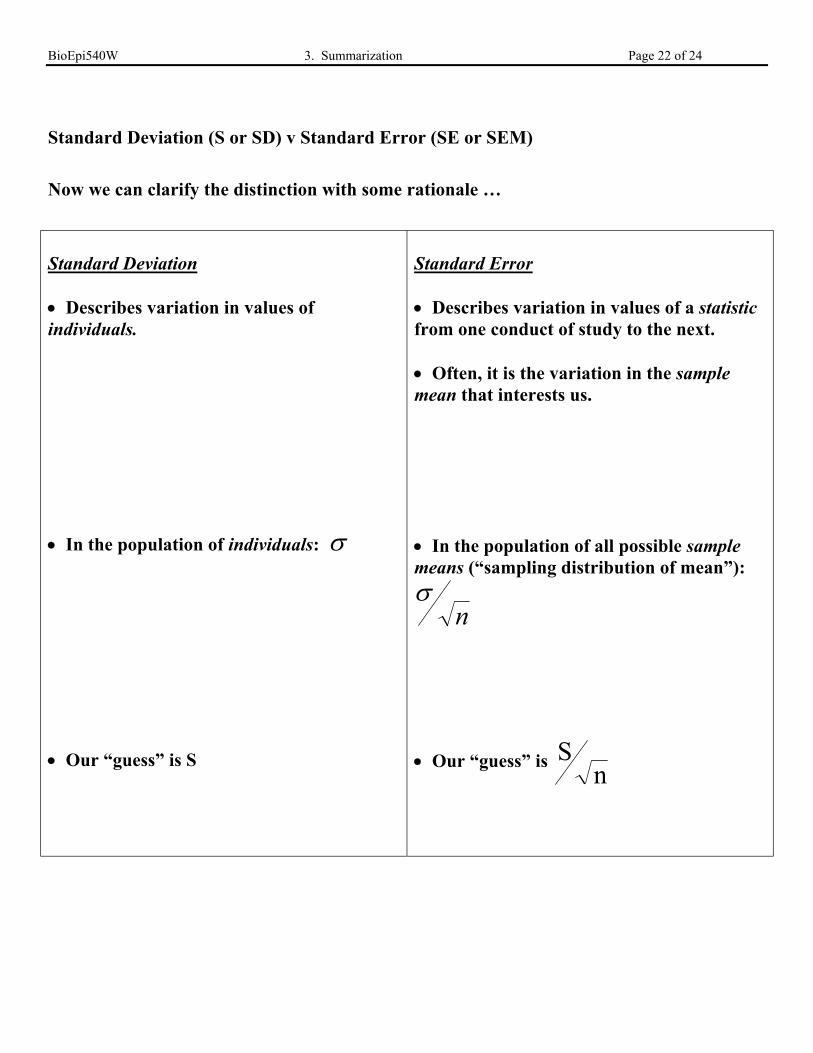
Standard Deviation (S or SD) v Standard Error (SE or SEM)

Now we can clarify the distinction with some rationale …

Standard Deviation

• Describes variation in values ofindividuals.

• In the population of individuals: σ

• Our “guess” is S

Standard Error

• Describes variation in values of a statisticfrom one conduct of study to the next.

• Often, it is the variation in the samplemean that interests us.

• In the population of all possible samplemeans (“sampling distribution of mean”):

σn

• Our “guess” is Sn


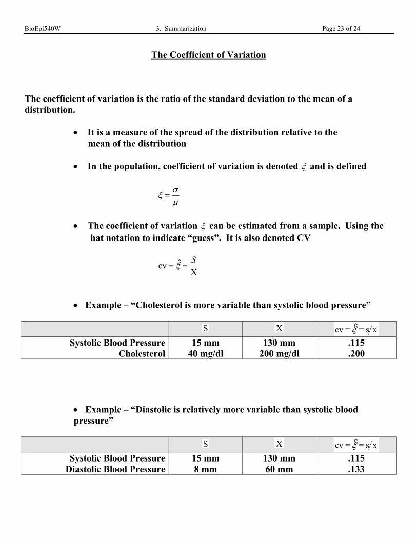
The Coefficient of Variation

The coefficient of variation is the ratio of the standard deviation to the mean of adistribution.

• It is a measure of the spread of the distribution relative to the mean of the distribution

• In the population, coefficient of variation is denoted ξ and is defined

ξ σµ

=

• The coefficient of variation ξ can be estimated from a sample. Using the hat notation to indicate “guess”. It is also denoted CV

cvX

= =$ξ S

• Example – “Cholesterol is more variable than systolic blood pressure”

S X cv = = s x$ξSystolic Blood Pressure 15 mm 130 mm .115

Cholesterol 40 mg/dl 200 mg/dl .200

• Example – “Diastolic is relatively more variable than systolic bloodpressure”

S X cv = = s x$ξSystolic Blood Pressure 15 mm 130 mm .115

Diastolic Blood Pressure 8 mm 60 mm .133


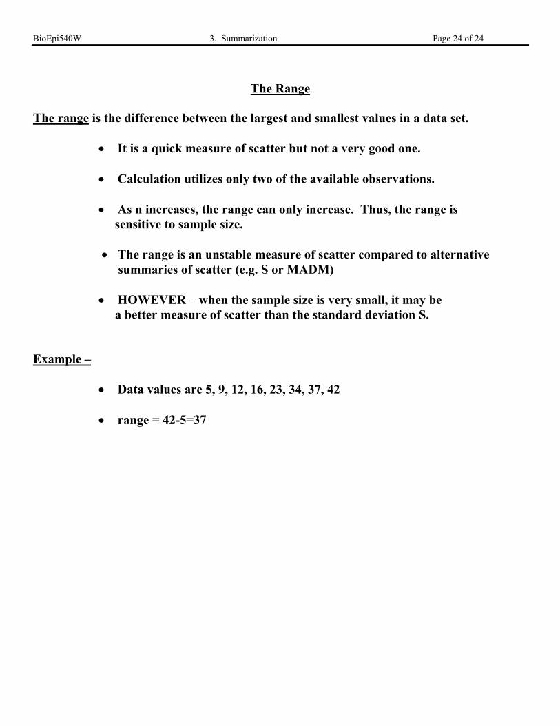
The Range

The range is the difference between the largest and smallest values in a data set.

• It is a quick measure of scatter but not a very good one.

• Calculation utilizes only two of the available observations.

• As n increases, the range can only increase. Thus, the range is sensitive to sample size.

• The range is an unstable measure of scatter compared to alternative summaries of scatter (e.g. S or MADM)

• HOWEVER – when the sample size is very small, it may be a better measure of scatter than the standard deviation S.

Example –

• Data values are 5, 9, 12, 16, 23, 34, 37, 42

• range = 42-5=37

Documents

3. Descriptive Statistics Summarization - UMasspeople.umass.edu/~biep540w/pdf/unit03.pdf · BioEpi540W 3. Summarization Page 3 of 24