バイオインフォマティクス特論3 ケーススタディ3-1. 記憶の保持 (2)

藤 博幸

事後予測分布パラメータの事後分布に従って、モデルがどんなデータを期待するかを予測する。

予測分布が観測されたデータと⼀致するかを確認することで、モデルの適切さを確認できる。

前回と同じ問題で事後予測を⾏う。

3-1. 記憶の保持3-1-1. 個⼈差を考えない場合3-1-2. 完全な個⼈差を考える場合3-1-3. 構造化された個⼈差を考える場合

3-1-1. 個人差を考えない場合「ベイズ統計で実践モデリング」 第10章 記憶の保持10.1 個⼈差を考えない場合

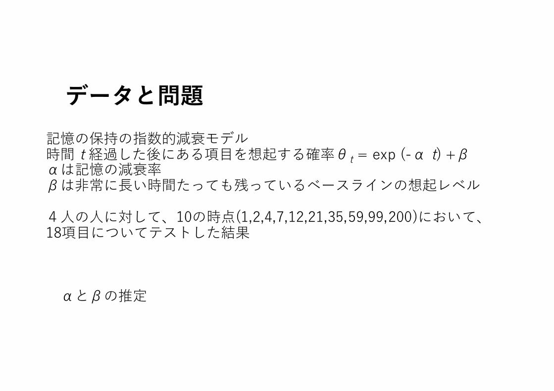
データと問題記憶の保持の指数的減衰モデル時間 t 経過した後にある項⽬を想起する確率θt = exp (-α t) +βαは記憶の減衰率βは⾮常に⻑い時間たっても残っているベースラインの想起レベル

４⼈の⼈に対して、10の時点(1,2,4,7,12,21,35,59,99,200)において、18項⽬についてテストした結果

αとβの推定

4名の実験参加者と10の時点の記憶保持データ

実験参加者 1 2 4 7 12 21 35 59 99 200

1 18 18 16 13 9 6 4 4 4 ?

2 17 13 9 6 4 4 4 4 4 ?

3 14 10 6 4 4 4 4 4 4 ?

4 ? ? ? ? ? ? ? ? ? ?

時点

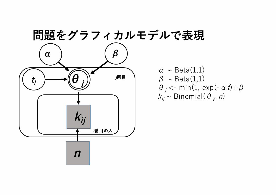
問題をグラフィカルモデルで表現

θj

kij

n

βα

tj j回⽬

i番⽬の⼈

α ~ Beta(1,1)β ~ Beta(1,1)θj <- min(1, exp(-αt)+βkij ~ Binomial(θj, n)

# Retention With No Individual Differencesmodel{

# Observed and Predicted Datafor (i in 1:ns){

for (j in 1:nt){k[i,j] ~ dbin(theta[i,j],n)predk[i,j] ~ dbin(theta[i,j],n)

}}# Retention Rate At Each Lag For Each Subject Decays Exponentiallyfor (i in 1:ns){

for (j in 1:nt){theta[i,j] <- min(1,exp(-alpha*t[j])+beta)

}}# Priorsalpha ~ dbeta(1,1)beta ~ dbeta(1,1)

}

Jagsでのモデルの記述 Retention_1.txt

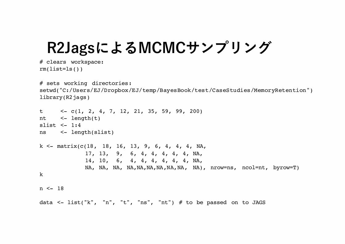
R2JagsによるMCMCサンプリング# clears workspace: rm(list=ls())

# sets working directories:setwd("C:/Users/EJ/Dropbox/EJ/temp/BayesBook/test/CaseStudies/MemoryRetention")library(R2jags)

t <- c(1, 2, 4, 7, 12, 21, 35, 59, 99, 200) nt <- length(t) slist <- 1:4 ns <- length(slist)

k <- matrix(c(18, 18, 16, 13, 9, 6, 4, 4, 4, NA,17, 13, 9, 6, 4, 4, 4, 4, 4, NA, 14, 10, 6, 4, 4, 4, 4, 4, 4, NA, NA, NA, NA, NA,NA,NA,NA,NA,NA, NA), nrow=ns, ncol=nt, byrow=T)

k n <- 18 data <- list("k", "n", "t", "ns", "nt") # to be passed on to JAGS

myinits <- list( list(alpha = 0.5, beta = 0.1))

# parameters to be monitored:parameters <- c("alpha", "beta", "predk")

# The following command calls JAGS with specific options.# For a detailed description see the R2jags documentation.samples <- jags(data, inits=myinits, parameters,

model.file ="Retention_1.txt",n.chains=1, n.iter=10000, n.burnin=1, n.thin=1, DIC=T)

# Now the values for the monitored parameters are in the "samples" object, # ready for inspection.

##############Fancy plots##################################################Figure 10.2

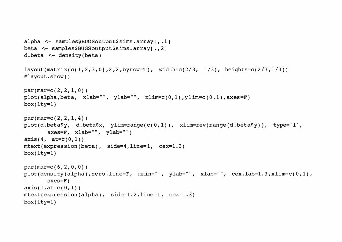
alpha <- samples$BUGSoutput$sims.array[,,1]beta <- samples$BUGSoutput$sims.array[,,2]d.beta <- density(beta)

alpha <- samples$BUGSoutput$sims.array[,,1]beta <- samples$BUGSoutput$sims.array[,,2]d.beta <- density(beta)

layout(matrix(c(1,2,3,0),2,2,byrow=T), width=c(2/3, 1/3), heights=c(2/3,1/3))#layout.show()

par(mar=c(2,2,1,0)) plot(alpha,beta, xlab="", ylab="", xlim=c(0,1),ylim=c(0,1),axes=F)box(lty=1)

par(mar=c(2,2,1,4)) plot(d.beta$y, d.beta$x, ylim=range(c(0,1)), xlim=rev(range(d.beta$y)), type='l',

axes=F, xlab="", ylab="")axis(4, at=c(0,1)) mtext(expression(beta), side=4,line=1, cex=1.3)box(lty=1)

par(mar=c(6,2,0,0)) plot(density(alpha),zero.line=F, main="", ylab="", xlab="", cex.lab=1.3,xlim=c(0,1),

axes=F)axis(1,at=c(0,1)) mtext(expression(alpha), side=1.2,line=1, cex=1.3)box(lty=1)

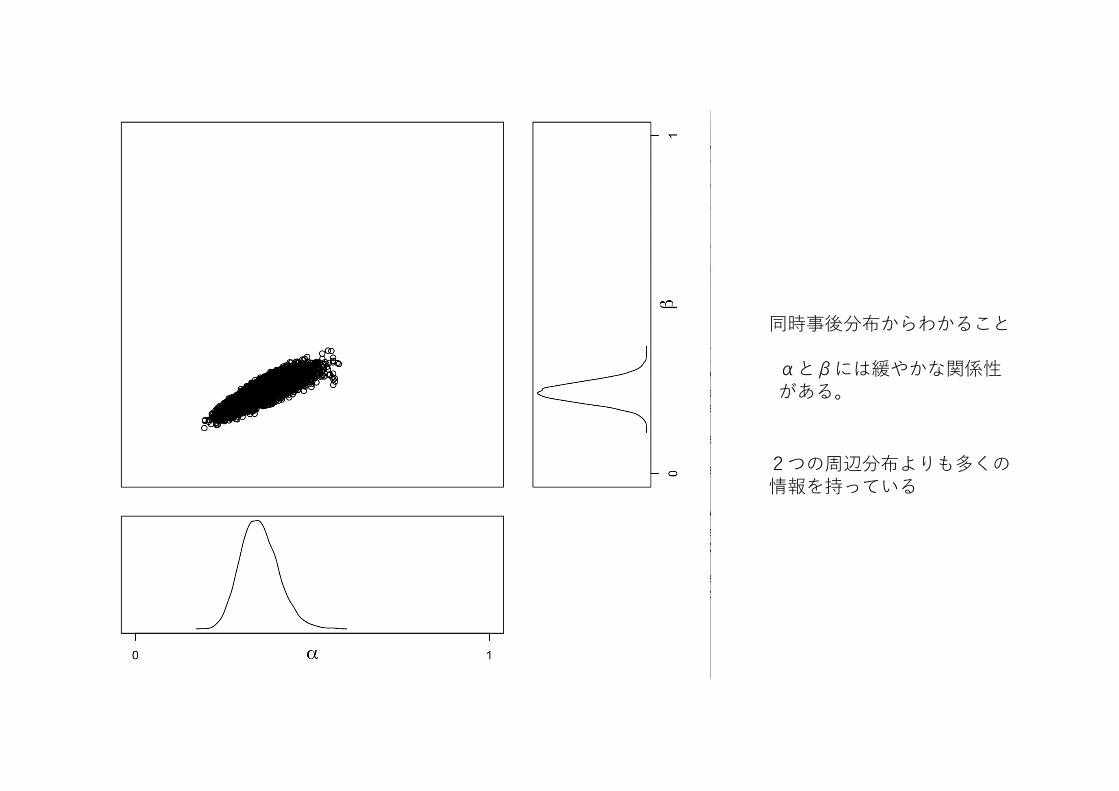
αとβには緩やかな関係性がある。

同時事後分布からわかること

２つの周辺分布よりも多くの情報を持っている

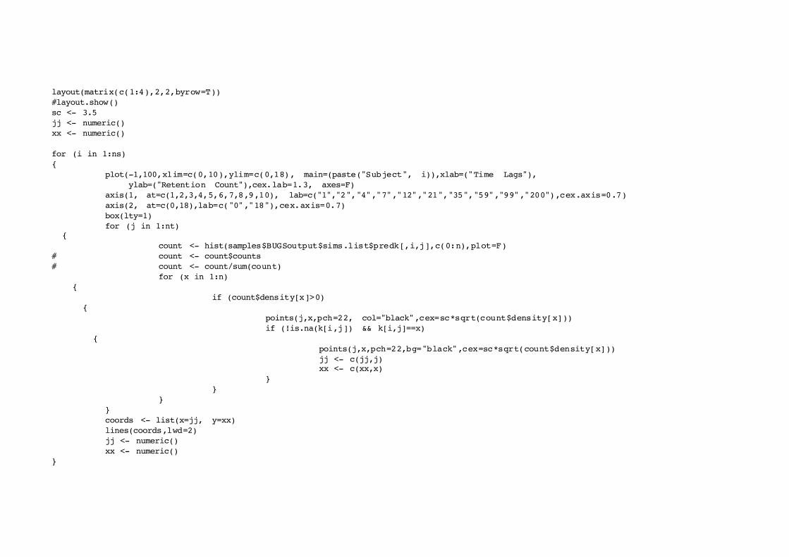
layout(matrix(c(1:4),2,2,byrow=T)) #layout.show() sc <- 3.5 jj <- numeric() xx <- numeric() for (i in 1:ns) { plot(-1,100,xlim=c(0,10),ylim=c(0,18), main=(paste("Subject", i)),xlab=("Time Lags"),

ylab=("Retention Count"),cex.lab=1.3, axes=F) axis(1, at=c(1,2,3,4,5,6,7,8,9,10), lab=c("1","2","4","7","12","21","35","59","99","200"),cex.axis=0.7) axis(2, at=c(0,18),lab=c("0","18"),cex.axis=0.7) box(lty=1) for (j in 1:nt) { count <- hist(samples$BUGSoutput$sims.list$predk[,i,j],c(0:n),plot=F) # count <- count$counts # count <- count/sum(count) for (x in 1:n) { if (count$density[x]>0) { points(j,x,pch=22, col="black",cex=sc*sqrt(count$density[x])) if (!is.na(k[i,j]) && k[i,j]==x) { points(j,x,pch=22,bg="black",cex=sc*sqrt(count$density[x])) jj <- c(jj,j) xx <- c(xx,x) } } } } coords <- list(x=jj, y=xx) lines(coords,lwd=2) jj <- numeric() xx <- numeric() }

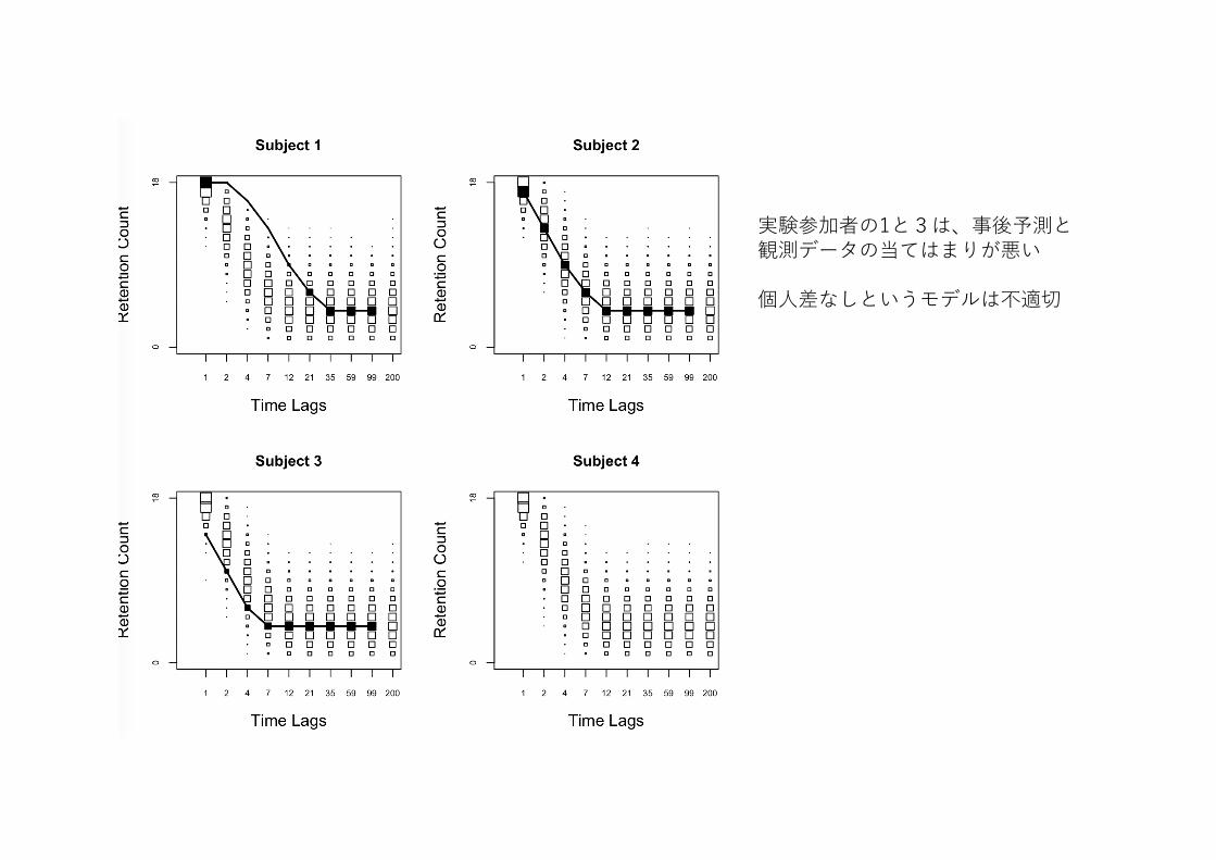
実験参加者の1と３は、事後予測と観測データの当てはまりが悪い

個⼈差なしというモデルは不適切

3-1-2.完全な個⼈差を考える場合「ベイズ統計で実践モデリング」 第10章 記憶の保持10.2 完全な個⼈差を考える場合

問題をグラフィカルモデルで表現

θij

kij

n

βiαi

tj

j回⽬

i番⽬の⼈

αi ~ Beta(1,1)βi ~ Beta(1,1)θij <- min(1, exp(-αit)+βikij ~ Binomial(θij, n)

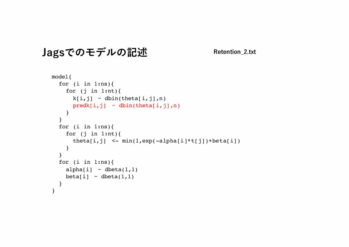
model{ for (i in 1:ns){ for (j in 1:nt){ k[i,j] ~ dbin(theta[i,j],n) predk[i,j] ~ dbin(theta[i,j],n) } } for (i in 1:ns){ for (j in 1:nt){ theta[i,j] <- min(1,exp(-alpha[i]*t[j])+beta[i]) } } for (i in 1:ns){ alpha[i] ~ dbeta(1,1) beta[i] ~ dbeta(1,1) } }

Jagsでのモデルの記述 Retention_2.txt

# clears workspace: rm(list=ls()) # sets working directories: setwd("C:/Users/EJ/Dropbox/EJ/temp/BayesBook/test/CaseStudies/MemoryRetention") library(R2jags) t <- c(1, 2, 4, 7, 12, 21, 35, 59, 99, 200) nt <- length(t) slist <- 1:4 ns <- length(slist) k <- matrix(c(18, 18, 16, 13, 9, 6, 4, 4, 4, NA,

17, 13, 9, 6, 4, 4, 4, 4, 4, NA, 14, 10, 6, 4, 4, 4, 4, 4, 4, NA, NA, NA, NA, NA,NA,NA,NA,NA,NA, NA), nrow=ns, ncol=nt, byrow=T)

k n <- 18 data <- list("k", "n", "t", "ns", "nt") # to be passed on to JAGS myinits <- list( list(alpha = rep(0.5,ns), beta = rep(0.1,ns)))

# parameters to be monitored:parameters <- c("alpha", "beta", "predk")

# The following command calls JAGS with specific options.# For a detailed description see the R2jags documentation.samples <- jags(data, inits=myinits, parameters,

model.file ="Retention_2.txt",n.chains=1, n.iter=10000, n.burnin=1, n.thin=1, DIC=T)

# Now the values for the monitored parameters are in the "samples" object, # ready for inspection.

##Figure 10.5n.iter <- 10000keepi <- 500keep <- sample(n.iter, keepi)

alpha1 <- samples$BUGSoutput$sims.array[,,1]alpha2 <- samples$BUGSoutput$sims.array[,,2]alpha3 <- samples$BUGSoutput$sims.array[,,3]alpha4 <- samples$BUGSoutput$sims.array[,,4]

beta1 <- samples$BUGSoutput$sims.array[,,5]beta2 <- samples$BUGSoutput$sims.array[,,6]beta3 <- samples$BUGSoutput$sims.array[,,7]beta4 <- samples$BUGSoutput$sims.array[,,8]d.beta1 <- density(beta1)d.beta2 <- density(beta2)d.beta3 <- density(beta3)d.beta4 <- density(beta4)

layout(matrix(c(1,2,3,0),2,2,byrow=T), width=c(2/3, 1/3), heights=c(2/3,1/3))#layout.show()

plot(alpha1[keep],beta1[keep], xlab="", ylab="", xlim=c(0,1), ylim=c(0,1), axes=F)points(alpha2[keep],beta2[keep], col="red")points(alpha3[keep],beta3[keep], col="green")points(alpha4[keep],beta4[keep],col="blue")box(lty=1)

par(mar=c(2,1,1,4))plot(d.beta1$y, d.beta1$x, ylim=range(c(0,1)), xlim=c(12,0),type='l', axes=F, xlab="", ylab="")#plot(d.beta1$y, d.beta1$x, ylim=range(c(0,1)), xlim=rev(range(d.beta1$y)),type='l', axes=F, xlab="", ylab="")lines(d.beta2$y, d.beta2$x, col="red")lines(d.beta3$y, d.beta3$x, col="green")lines(d.beta4$y, d.beta4$x, col="blue")axis(4, at=c(0,1))mtext(expression(beta), side=4,line=1, cex=1.3)box(lty=1)

par(mar=c(6,2,0,0))plot(density(alpha1),zero.line=F ,main="", ylab="", xlab="", cex.lab=1.3,xlim=c(0,1), axes=F)lines(density(alpha2), col="red")lines(density(alpha3), col="green")lines(density(alpha4),col="blue")axis(1,at=c(0,1))mtext(expression(alpha), side=1.2,line=1, cex=1.3)box(lty=1)

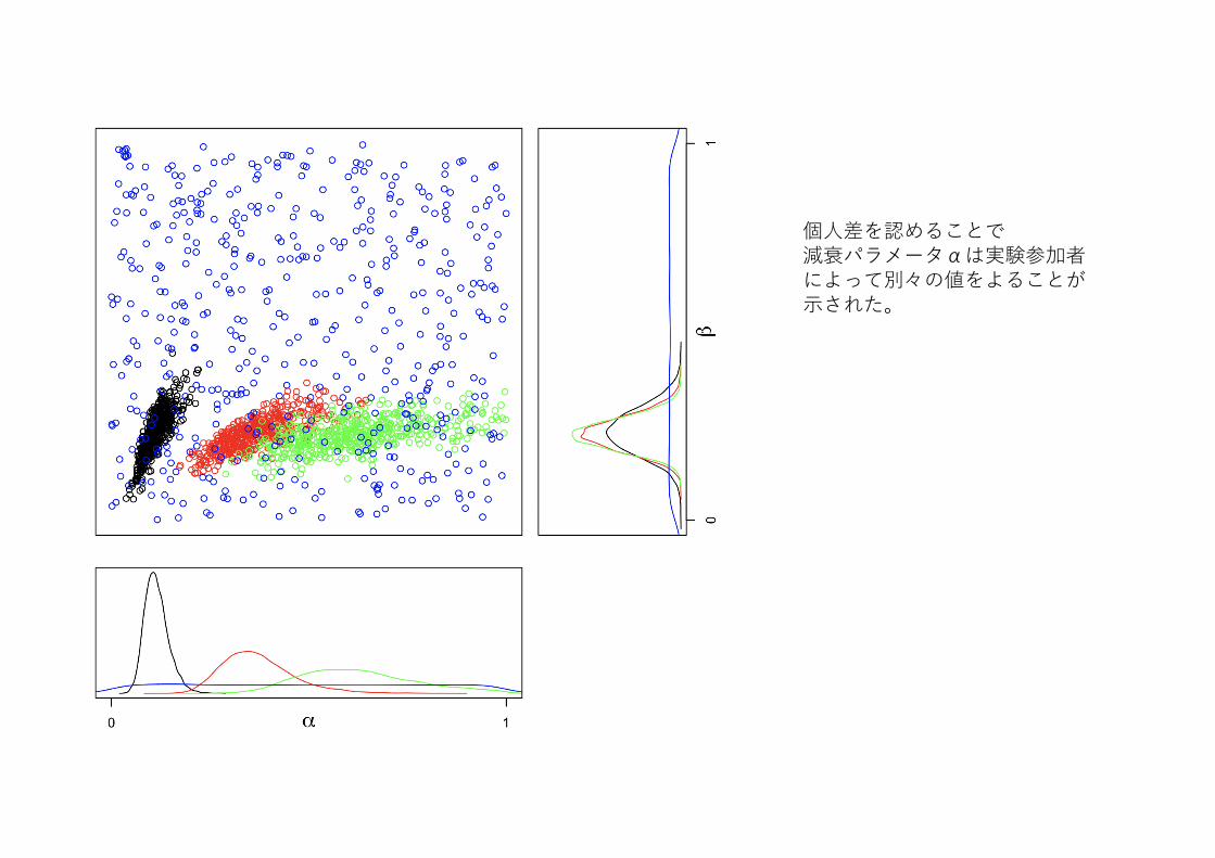
個⼈差を認めることで減衰パラメータαは実験参加者によって別々の値をよることが⽰された。

layout(matrix(c(1:4),2,2,byrow=T)) #layout.show() sc <- 3.5 jj <- numeric() xx <- numeric() for (i in 1:ns) { plot(-1,100,xlim=c(0,10),ylim=c(0,18), main=(paste("Subject", i)),xlab=("Time Lags"), ylab=("Retention Count"),cex.lab=1.3, axes axis(1, at=c(1,2,3,4,5,6,7,8,9,10), lab=c("1","2","4","7","12","21","35","59","99","200"),cex.axis=0.7) axis(2, at=c(0,18),lab=c("0","18"),cex.axis=0.7) box(lty=1) for (j in 1:nt) {

j1 <- i+9 + (j-1)*4 count <- hist(samples$BUGSoutput$sims.list$predk[,i,j],c(0:n),plot=F) # count <- count$counts # count <- count/sum(count) for (x in 1:n){ if (count$density[x]>0){ points(j,x,pch=22, col="black",cex=sc*sqrt(count$density[x])) if (!is.na(k[i,j]) && k[i,j]==x){ points(j,x,pch=22,bg="black",cex=sc*sqrt(count$density[x])) jj <- c(jj,j) xx <- c(xx,x) } } } } coords <- list(x=jj, y=xx) lines(coords,lwd=2) jj <- numeric() xx <- numeric() }

実験参加者1~3については観測データと予測分布が対応し、モデルの妥当性を⽰している

実験参加者4については、利⽤できる情報はαとβの事前分布のみであることから、予測分布には役に⽴つ情報は含まれていない

3-1-3. 構造化された個⼈差を考える場合「ベイズ統計で実践モデリング」 第10章 記憶の保持10.3 構造化された個⼈差を考える場合

問題をグラフィカルモデルで表現

θij

kij

n

βiαi

tj

j回⽬

i番⽬の⼈

μα~Beta(1,1)λα~Gammma(.001, .001)μβ~Beta(1,1) λβ~Gammma(.001, .001)

αi ~ Gaussian(μα, λα)r(0,1)βi ~ Gaussian(μβ, λβ)r(0,1)θij <- min(1, exp(-αit)+βikij ~ Binomial(θij, n)

μα

λα

μβ

λβ

model{ for (i in 1:ns){ for (j in 1:nt){ k[i,j] ~ dbin(theta[i,j],n) predk[i,j] ~ dbin(theta[i,j],n) } } for (i in 1:ns){ for (j in 1:nt){ theta[i,j] <- min(1,exp(-alpha[i]*t[j])+beta[i]) } } for (i in 1:ns){ alpha[i] ~ dnorm(alphamu,alphalambda)I(0,1) beta[i] ~ dnorm(betamu,betalambda)I(0,1) } alphamu ~ dbeta(1,1) alphalambda ~ dgamma(.001,.001)I(.001,) alphasigma <- 1/sqrt(alphalambda) betamu ~ dbeta(1,1) betalambda ~ dgamma(.001,.001)I(.001,) betasigma <- 1/sqrt(betalambda) }

Jagsでのモデルの記述 Retention_3.txt

rm(list=ls())

# sets working directories:setwd("C:/Users/EJ/Dropbox/EJ/temp/BayesBook/test/CaseStudies/MemoryRetention")library(R2jags)

t <- c(1, 2, 4, 7, 12, 21, 35, 59, 99, 200)nt <- length(t)slist <- 1:4ns <- length(slist)

k <- matrix(c(18, 18, 16, 13, 9, 6, 4, 4, 4, NA,17, 13, 9, 6, 4, 4, 4, 4, 4, NA,14, 10, 6, 4, 4, 4, 4, 4, 4, NA,NA, NA, NA, NA,NA,NA,NA,NA,NA, NA), nrow=ns, ncol=nt, byrow=T)

k

n <- 18

data <- list("k", "n", "t", "ns", "nt") # to be passed on to JAGSmyinits <- list(list(alphamu = 0.5, alphalambda = 1, betamu = 0.5, betalambda = 1, alpha = rep(0.5,ns), beta = rep(0.1,ns)))

# parameters to be monitored:parameters <- c("alpha", "beta", "predk")

# The following command calls JAGS with specific options.# For a detailed description see the R2jags documentation.samples <- jags(data, inits=myinits, parameters,

model.file ="Retention_3.txt",n.chains=1, n.iter=10000, n.burnin=1, n.thin=1, DIC=T)

n.iter <- 10000keepi <- 500keep <- sample(n.iter, keepi)

alpha1 <- samples$BUGSoutput$sims.array[,,1]alpha2 <- samples$BUGSoutput$sims.array[,,2]alpha3 <- samples$BUGSoutput$sims.array[,,3]alpha4 <- samples$BUGSoutput$sims.array[,,4]

beta1 <- samples$BUGSoutput$sims.array[,,5]beta2 <- samples$BUGSoutput$sims.array[,,6]beta3 <- samples$BUGSoutput$sims.array[,,7]beta4 <- samples$BUGSoutput$sims.array[,,8]d.beta1 <- density(beta1)d.beta2 <- density(beta2)d.beta3 <- density(beta3)d.beta4 <- density(beta4)

layout(matrix(c(1,2,3,0),2,2,byrow=T), width=c(2/3, 1/3), heights=c(2/3,1/3))

par(mar=c(2,2,1,0))plot(alpha1[keep],beta1[keep], xlab="", ylab="", xlim=c(0,1), ylim=c(0,1), axes=F)points(alpha2[keep],beta2[keep], col="red")points(alpha3[keep],beta3[keep], col="green")points(alpha4[keep],beta4[keep],col="blue")box(lty=1)

par(mar=c(2,1,1,4))plot(d.beta1$y, d.beta1$x, ylim=range(c(0,1)), xlim=c(12,0),type='l', axes=F, xlab="", ylab="")#plot(d.beta1$y, d.beta1$x, ylim=range(c(0,1)), xlim=rev(range(d.beta1$y)),type='l', axes=F, xlab="", ylab="")lines(d.beta2$y, d.beta2$x, col="red")lines(d.beta3$y, d.beta3$x, col="green")lines(d.beta4$y, d.beta4$x, col="blue")axis(4, at=c(0,1))mtext(expression(beta), side=4,line=1, cex=1.3)box(lty=1)

par(mar=c(6,2,0,0))plot(density(alpha1),zero.line=F ,main="", ylab="", xlab="", cex.lab=1.3,xlim=c(0,1), axes=F)lines(density(alpha2), col="red")lines(density(alpha3), col="green")lines(density(alpha4),col="blue")axis(1,at=c(0,1))mtext(expression(alpha), side=1.2,line=1, cex=1.3)box(lty=1)

layout(matrix(c(1:4),2,2,byrow=T)) #layout.show() sc <- 3.5 jj <- numeric() xx <- numeric() for (i in 1:ns) { plot(-1,100,xlim=c(0,10),ylim=c(0,18), main=(paste("Subject", i)),xlab=("Time Lags"),

ylab=("Retention Count"),cex.lab=1.3, axes=F) axis(1, at=c(1,2,3,4,5,6,7,8,9,10), lab=c("1","2","4","7","12","21","35","59","99","200"),cex.axis=0.7) axis(2, at=c(0,18),lab=c("0","18"),cex.axis=0.7) box(lty=1) for (j in 1:nt) { count <- hist(samples$BUGSoutput$sims.list$predk[,i,j],c(0:n),plot=F) # count <- count$counts # count <- count/sum(count) for (x in 1:n){ if (count$density[x]>0){ points(j,x,pch=22, col="black",cex=sc*sqrt(count$density[x])) if (!is.na(k[i,j]) && k[i,j]==x){ points(j,x,pch=22,bg="black",cex=sc*sqrt(count$density[x])) jj <- c(jj,j) xx <- c(xx,x) } } } } coords <- list(x=jj, y=xx) lines(coords,lwd=2) jj <- numeric() xx <- numeric() }

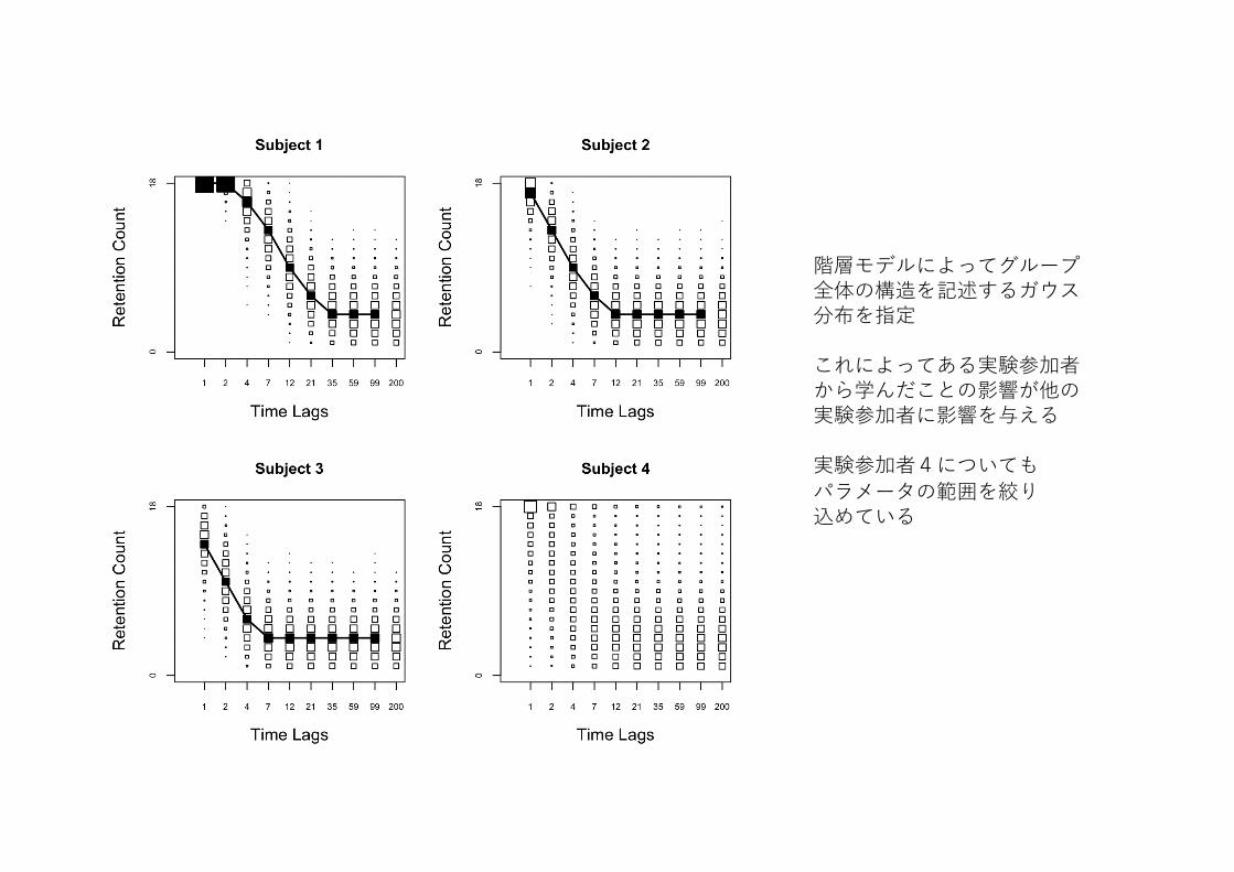
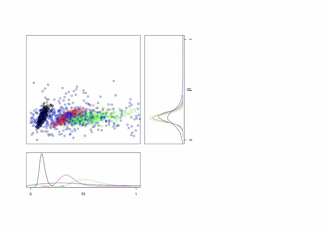
階層モデルによってグループ全体の構造を記述するガウス分布を指定

これによってある実験参加者から学んだことの影響が他の実験参加者に影響を与える

実験参加者４についてもパラメータの範囲を絞り込めている