1

4. Forecasting with ARMA models 

MSE optimal forecasts

• Let      denote a one‐step ahead forecast given information Ft .  For ARMA models, 

• The optimal MSE forecast minimizes

1tY

211t tE Y Y

1, ,...t t tF Y Y

2

• MSE is a convenient forecast evaluation that has nice theoretical properties.

• MSE is not always a good way to evaluate forecasts from an economic perspective. 

– It is symmetric.  Do you care the same about underestimating the time to walk to the bus vs. overestimating?

– In general, non‐linear payoff functions are not optimized by MSE.  

The optimal MSE forecast is the conditional expectation

• To see this, let g(Xt) denote any other forecast.

• The middle (cross product) term has expectation zero by the Law of Iterated Expectations (LIE)

22

1

2

1

1

1

1

1 1 1

2

1

1

|

|

|

2* |

|

|

t t tt t t

t t t t t t t t

t

t t

t

t t

Y E Y X

Y E Y X Y

E Y g X E E Y X g X

E Y X g X

E Y X g

X

X

E

E

YE E

|E Y E E Y X

t

1 1

only randomthing giv

1 1

en X

| 00| |tt t tt t t t t tE Y X g XE E YY E Y E X g XXX

3

• So the middle term vanishes and we are left with:

• The smallest the second term can be is zero and it is zero only when

• So the optimal MSE forecast is the conditional expectation.  

2

11

2 2

1 1 | |t t t tt tt tE Y X gE Y g X E EY Y XE X

1 |t t tE Y X g X

Restricting our attention to linear models, a similar result holds for Least Squares estimators

• Let                             so that         is the linear projection of Yt+1 on Xt, or the least squares solution.   

• A nearly identical proof shows that the linear projection provides the MSE optimal forecast in the class of linear predictors.  

• Let       denote the least squares solution and  let       denote any other linear combination.

1 0t t tE Y X X tX

tX

tX g

4

• The middle term again has expectation zero.

• The resulting expression 

is minimized when 

2

2

1

1

2

1

2

1

2*

t t t

t t

t

t

t t t

t

t

t

t Y X

Y X

E Y X g E

E E Y

X X g

X X g

X X gE

X

1 1

1 0 0

t t t

t

t t t t

t t

E EX XY X Y X

Y

g X g

X gE X g

1

2 2 2

1 t tt t ttE Y Y XX g E E X X g

t tX X g

• So if the true conditional expectation is linear then the linear model is the optimal MSE. 

• If the true model is non‐linear, then the linear model is the best linear predictor.  

5

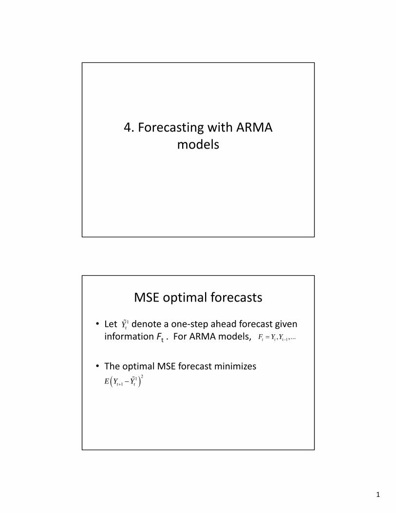
Forecasting ARMA models

• Consider the ARMA model:

where

and 

• If the model is weakly stationary we get:

or

where        

t tL Y L

21 21 ... p

pL L L L

21 21 ... q

qL L L L

1 1

t tL L Y L L

0 1 0

t j t jj

Y

Multi‐step ahead forecast

• Or,  

• If the ’s are independent, then conditional on past ’s, future ’s have expectation zero:

• The forecast error is

• Since the forecast errors are uncorrelated with the “X’s” use to predict, this is the best linear predictor.

1| ,t k t t j t k jj k

E Y

1

0

future after time t past, before time t

k

t k j t k j j t k jj j k

Y

1

0

kk

t k t j t k jj

E Y Y

6

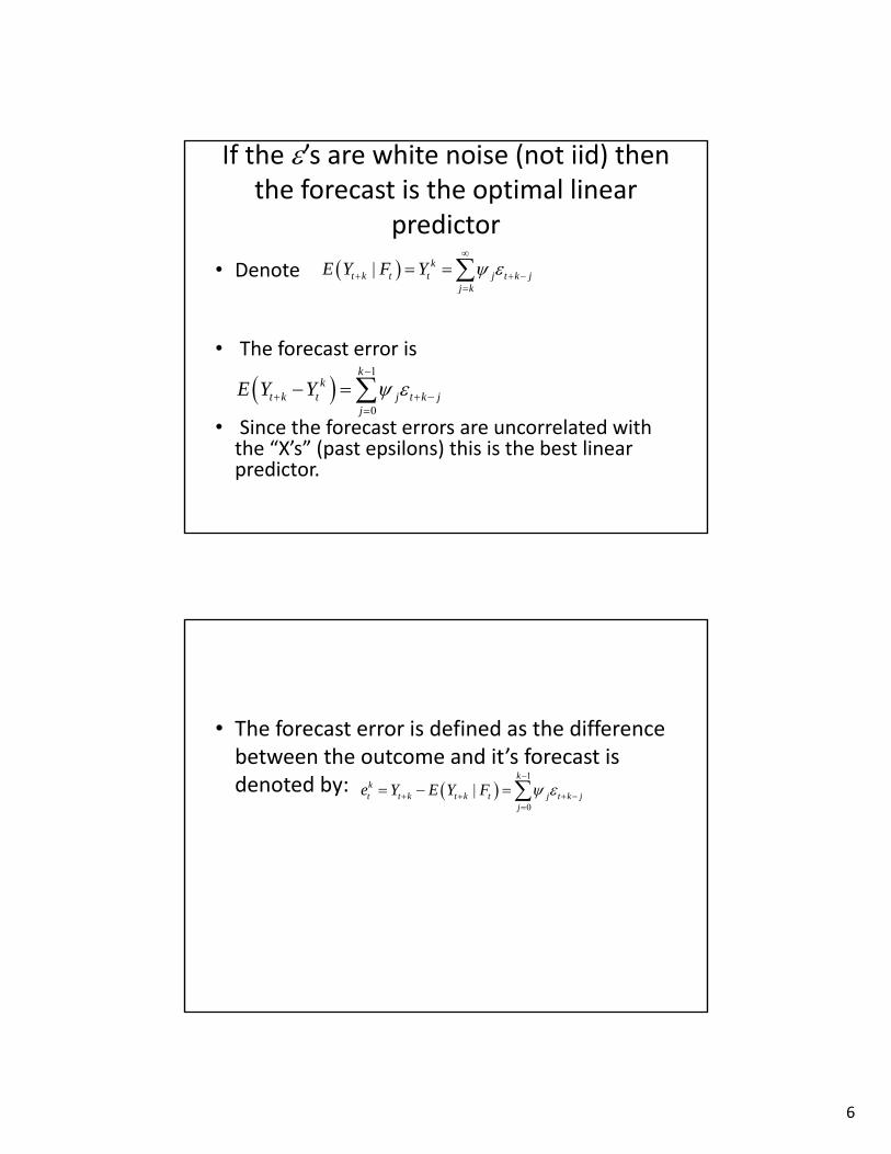
If the ’s are white noise (not iid) then the forecast is the optimal linear 

predictor

• Denote 

• The forecast error is

• Since the forecast errors are uncorrelated with the “X’s” (past epsilons) this is the best linear predictor.

| kt k t t j t k j

j k

E Y F Y

1

0

kk

t k t j t k jj

E Y Y

• The forecast error is defined as the difference between the outcome and it’s forecast is denoted by:

1

0

|k

kt t k t k t j t k j

j

e Y E Y F

7

• The k‐step ahead forecast error variance is then given by:

• If the errors are Gaussian then the 95% prediction interval is given by:

1 1

2 2

0 0

k kkt j t k j j

j j

Var e Var

12

0

2k

kt j

j

Y

Example

• Consider the AR(1) model

• Pre‐multiply both sides of Yt+k by:

yielding

or

01 t tL Y

2 2 1 11 ... k kL L L

1 1

00 0

k kk j j

t k t t k jj j

Y Y

1 1

00 0

1k k

k k j jt k t k j

j j

L Y

8

• The k‐step ahead forecast is:

• The forecast error is

• The forecast error variance is:

1 1

00 0

|k k

k j j kt k t t t k j t

j j

E Y F Y E Y

1

0

kj

t k jj

1 12 2

0 0

k kj j

t jj j

Var

• Notice that we could pre‐multiply by 

regardless of whether  is

less than one (we didn’t actually use the 

inverse operator).

2 2 1 11 ... k kL L L

9

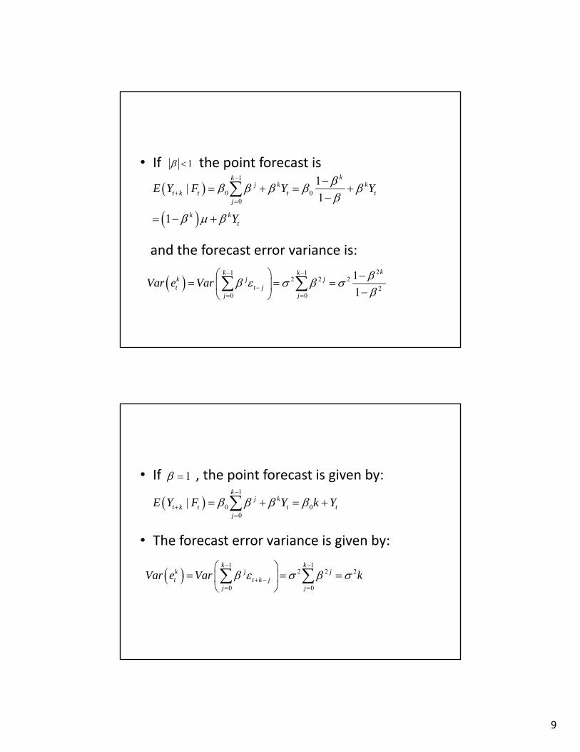
• If           the point forecast is

and the forecast error variance is:

1

1

0 00

1|

1

1

kkj k k

t k t t tj

k kt

E Y F Y Y

Y

21 1

2 2 22

0 0

1

1

kk kk j jt t j

j j

Var e Var

• If          , the point forecast is given by:

• The forecast error variance is given by: 

1

1 1

2 2 2

0 0

k kk j jt t k j

j j

Var e Var k

1

0 00

|k

j kt k t t t

j

E Y F Y k Y

10

A simple algorithm for multi‐step ahead forecasts

• 1 step:

• 2 step

• 3 step

1 1 11 1

|p q

t t j t j j t jj i

E Y F Y

2 1 1 2 1 1 22 1

One-step ahead forecast 0

1 t+1 t 2 22 1

| E | |

E Y |F

p q

t t t t j t j t t j t ij i

p q

j t j j t ij i

E Y F Y F Y E F

Y

3 1 2 2 1 3 33 3

| | |p q

t t t t t t j t j j t jj i

E Y F E Y F E Y F Y

• So once you have the one‐step you can get the two step, once you have the two‐step, you can get the three‐step and so on.  

• Plug in conditional expected values for future values of Y and zero for the expectation of future values of .  Plug in know past values for values of Y and  at or before time t. 

11

5. Maximum Likelihood Estimation

• Let’s start with a simple example.  

• Suppose that we take an iid sample of size 10 of whether a voter will vote for candidate A.  

• Suppose the data look like this:

1 0 1 1 1 0 0 1 0 1    where a 1 denotes “favor candidate A”.

• Let p denote the true fraction of voters that favor candidate A.  p is the parameter we want to estimate.

• If we knew p, how likely would it be to observe this sequence of data?

• Well, they are all independent and identically distributed.1 0 1 1 1 0 0 1 0 1The joint probability that x1=1, x2=0, x3=1… is given by:p(1‐p)ppp(1‐p)(1‐p)p(1‐p)p=p6(1‐p)4

12

• More generally, for a sample of size n we can write the probability of observing the sample as

• This is simply the joint probability of n outcomes. 

01 1nnp p

• For a given value of p,                                       tells us how likely it is to observe this particular data set. We therefore call this the likelihood function.

• The goal of maximum likelihood is to find the parameter value p that maximizes the likelihood function.

• In doing so we are finding the parameter value that makes it most likely that we observe our given sample.

01| 1nnL data p p p

13

• The log function is a monotonically increasing function.  This means that the value of p that maximizes the likelihood function L is the same as the value of p that maximizes the log of the likelihood function.

1 0| ln ln ln 1data p L n p n p L

• We can maximize the likelihood by taking the derivative and setting it to zero. 

• The p that maximizes the log likelihood function will be our estimate of p so we denote it by  p

14

• Taking the derivative and setting to zero yields:

• The solution is:

01|

0(1 )

d p data nn

dp p p

L

1 1

0 1

ˆn n

pn n n

• For continuous random variables the density function describes probabilities.

• Let          denote a density function that depends on a possible vector of parameters (i.e. for the normal it depends on the mean and variance).

|f

15

• If we take an iid sample of a continuous random variable then the likelihood of observing the sample is given by the product of the marginal densities.

1 2 1 2, , , | | | |n nf y y y f y f y f y

• It is convenient to take the log of the joint density function in which case we get:

• As before, the value of  that maximizes the function f will also maximize ln(f) and is called the Maximum Likelihood Estimate    .

1 21

ln , , , | ln |n

n ii

f y y y f y

16

• Example:  iid Normal likelihood function.

(on white board)

How do we set up the likelihood for dependent time series data?

• The factorization of the likelihood into the product of marginal densities relied on an iid sample of data which is clearly not true for dependent time series data.

• Fact:  without any loss of generality, the joint density function                                can always be expressed as:

1 1, , , |T Tf y y y

1 1 1 2 1 1 2 3 1

2 3 4 1 2 1 1

, , , | | , ,..., ; | , ,..., ;

| , ,..., ; ... | ; ;

T T T T T T T T

T T T

f y y y f y y y y f y y y y

f y y y y f y y f y

17

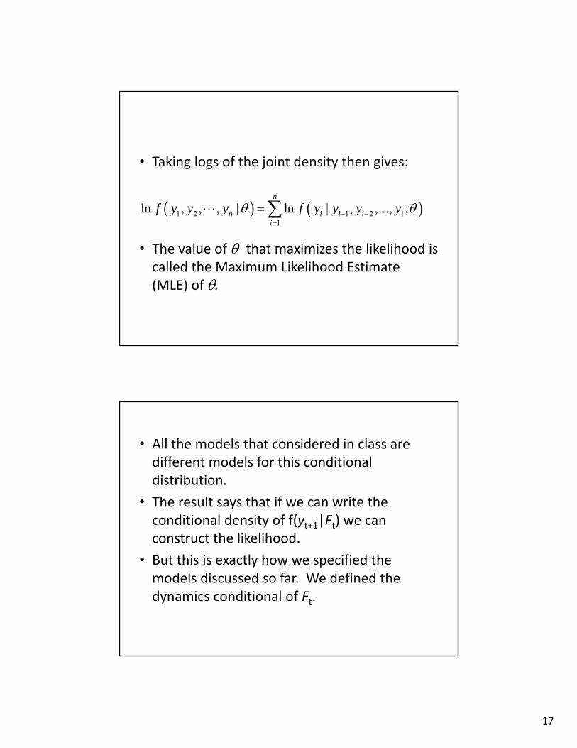
• Taking logs of the joint density then gives:

• The value of that maximizes the likelihood is called the Maximum Likelihood Estimate (MLE) of 

1 2 1 2 11

ln , , , | ln | , ,..., ;n

n i i ii

f y y y f y y y y

• All the models that considered in class are different models for this conditional distribution. 

• The result says that if we can write the conditional density of f(yt+1|Ft) we can construct the likelihood.

• But this is exactly how we specified the models discussed so far.  We defined the dynamics conditional of Ft.  

18

• AR(1) model likelihood under Gaussian errors.

(on white board)

Variance of maximum likelihood parameter estimates

• The value of  that maximizes the likelihood is our estimate, but how accurate is the estimate?

• If the assumed distribution is correct then the variance covariance matrix of the parameter estimates is given by inverse of the information matrix denoted by I‐1.

19

• Write the log likelihood function as:                 where

• There are two ways to estimate the information matrix:

1) 

2) 

22

ˆ ˆ21

1 1ˆ | |T

td

t

d ld LI

T d d T d d

ˆ ˆ1

1ˆ | |T

t top

t

dl dlI

T d d

T

ttl

1

L

1 2 1ln | , ,..., ;t t t tl f y y y y

Constructing the information matrix

• The if 0 is the true parameter value, the distribution of the parameter estimates is given by:

• Where  is one of the two estimates       or

.

11ˆ ˆ~ ,oN IT

2dI

opI

I

20

• When the model is correctly specified the two estimate of the information matrix are the same in large samples.   In small samples they will differ a little although neither is preferred.

• There are several ways the model can be wrong.  

– First, we could misspecify the dynamics (i.e. have the wrong AR model)

– Second, we could use the wrong shape for the conditional distribution (i.e. use a Normal when we should have used a t‐distribution)

Getting the standard errors right

• Interestingly, if we have the dynamics right but falsely assume Normality, the parameter estimates are still consistent under very general conditions.  

• The standard errors will be wrong, however.

• The good news is that we know how to fix them.

21

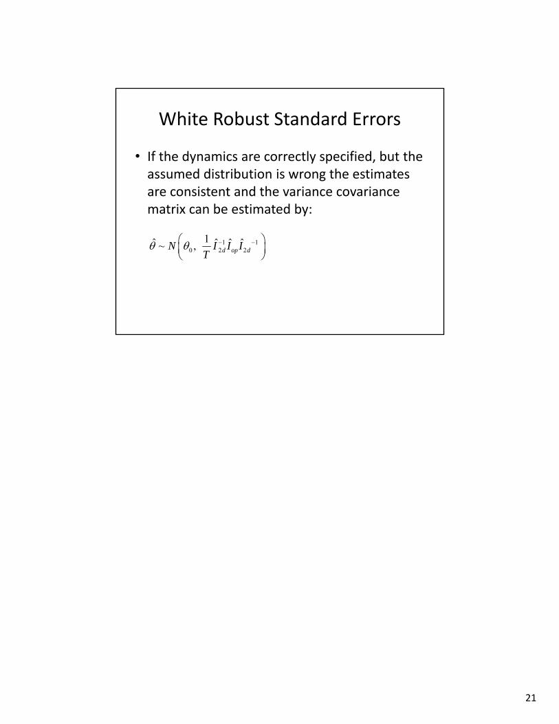
White Robust Standard Errors

• If the dynamics are correctly specified, but the assumed distribution is wrong the estimates are consistent and the variance covariance matrix can be estimated by:

1 10 2 2

1ˆ ˆ ˆ ˆ~ , d op dN I I IT