4583-4593

7/26/2019 4583-4593

http://slidepdf.com/reader/full/4583-4593 1/11

A new cohesive zone model for mixed mode interface

fracture in bimaterials

Yuval Freed *, Leslie Banks-Sills

The Dreszer Fracture Mechanics Laboratory, School of Mechanical Engineering, The Fleischman Faculty of Engineering, Tel Aviv University, 69978 Ramat Aviv, Israel

a r t i c l e i n f o

Article history:

Received 16 December 2007

Received in revised form 14 April 2008

Accepted 28 April 2008

Available online 6 May 2008

Keywords:

Cohesive zone modeling

Constitutive modeling

Finite element analysis

Interface fracture

Mixed mode fracture

a b s t r a c t

A new two-dimensional cohesive zone model which is suitable for the prediction of mixed

mode interface fracture in bimaterials is presented. The model accounts for the well known

fact that the interfacial fracture toughness is not a constant, but a function of the mode

mixity. Within the framework of this model, the cohesive energy and the cohesive strength

are not chosen to be constant, but rather functions of the mode mixity. A polynomial cohe-

sive zone model is derived in light of analytical and experimental observations of interface

cracks. The validity of the new cohesive law is examined by analyzing double cantilever

beam and Brazilian disk specimens. The methodology to determine the parameters of

the model is outlined and a failure criterion for a pair of ceramic clays is suggested.

2008 Elsevier Ltd. All rights reserved.

1. Introduction

Interfaces have been investigated in several ways in the past. One possibility is to assume that the two materials are per-

fectly bonded. With this approach, a conservative integral may be employed to obtain the stress intensity factors and the

corresponding energy release rate (see for example [1]). However, if the crack advances quasi-statically, the interface may

be simulated as a very thin continuum region with graded properties [2], as a narrow strip of springs [3–7] or using a cohe-

sive zone model. The latter approach was first proposed by Barenblatt [8,9] and Dugdale [10] as an alternative approach to

singular crack tip behavior. With this concept, the stresses ahead of the crack tip are bounded, and a traction–separation law

is used to describe the fracture process.

Because of its versatility, cohesive zone models are increasingly applied in many engineering fields. For instance, cohesive

zone models have been used to study crack tip plasticity [11], creep under static and fatigue loading [12], adhesive bonded

joints [13], crack bridging [14], and interface cracks in bimaterials [15]. As discussed by Li and Chandra [11], a great advan-

tage of cohesive zone models is that they are able to represent several micromechanical mechanisms in the vicinity of thecrack tip. In addition, they can be easily implemented in a numerical framework. For a detailed review on the applications of

cohesive zone models, the reader is directed to Chandra et al. [16].

There are several cohesive zone models that deal with mixed mode deformation and interface cracks. In general, these

laws are written separately for each mode and then coupled together, either by defining coupling parameters or by using

an effective displacement. As an example of the former approach, the cohesive law presented by Xu and Needleman [17],

which was implemented to investigate particle–matrix decohesion, is governed by two coupling parameters, which relate

the ratio between the energy release rates of pure modes I and II and the corresponding displacements. However, it was

shown by van den Bosch et al. [18] that this model does not describe realistic mixed mode behavior unless the energy release

0013-7944/$ - see front matter 2008 Elsevier Ltd. All rights reserved.doi:10.1016/j.engfracmech.2008.04.013

* Corresponding author. Tel.: +972 3 640 5581; fax: +972 3 640 7617.

E-mail address: [email protected] (Y. Freed).

Engineering Fracture Mechanics 75 (2008) 4583–4593

Contents lists available at ScienceDirect

Engineering Fracture Mechanics

j o u r n a l h o m e p a g e : w w w . e l s e v i e r . c o m / l o c at e / e n g f r a c m e c h

mailto:[email protected]

http://www.sciencedirect.com/science/journal/00137944

http://www.elsevier.com/locate/engfracmech

http://www.elsevier.com/locate/engfracmech

http://www.sciencedirect.com/science/journal/00137944

mailto:[email protected]

7/26/2019 4583-4593


rates of both modes are equal. Unfortunately, this assumption is not generally correct. To overcome this problem, a non-

dimensional effective relative crack displacement was assumed by many investigators to obtain mixed mode interface

behavior (see for instance [19–22]). As discussed by Zhang and Paulino [23] and van den Bosch et al. [18], a major difficulty

arises when considering an effective relative crack displacement; it results in a constant energy of separation, which is not

realistic in the case of interface cracks. It is well known that the interfacial fracture toughness is not a constant, but a function

of the mode mixity [24,1,25]. To this end, in several investigations a variable interfacial fracture toughness has been incor-

porated into cohesive zone models (see for example [26,27]). An ellipse-shape criterion was assumed to account for the ef-

fect of the mode mixity. Although this failure criterion is widely used by many researchers for different applications of

unidirectional composites, this criterion might not be sufficiently accurate for certain cases of mixed mode interface cracks,

especially between dissimilar isotropic materials. To overcome this problem, Hutchinson and Suo [24] introduced a com-

pletely different mixed mode failure criterion which was found to be suitable for interface cracks between dissimilar isotro-

pic materials, as well as for laminated composites [28].

The main objective of this study is to introduce a new cohesive zone model which is capable of describing the dependence

of the model parameters upon the mode mixity. Within the scheme of this model, the cohesive energy is not constant, but a

function of the mode mixity. A polynomial cohesive zone model is derived in light of analytical and experimental observa-

tions of interface cracks [24,1,29,28,30]. The second objective of this study is to propose a methodology for determining the

model parameters from experimental data. To this end, a failure criterion is obtained according to the new cohesive law.

The present paper is organized as follows. First, several important concepts regarding fracture mechanics of interface

cracks are briefly discussed in Section 2. The constitutive equations of the proposed cohesive zone model are described in

Section 3. The corresponding tangent modulus matrix is derived, as well as a numerical scheme of an interface element.

In Section 4, the validity of the new cohesive law is examined. To this end, double cantilever beam and Brazilian disk spec-

imens are analyzed. Finally, a methodology to determine the parameters of the model is outlined.

2. Review of fracture mechanics of interface cracks

In this section, several important concepts of fracture mechanics of interface cracks are briefly outlined. An assumption of

small scale plastic and contact zones is invoked. Consequently, the theory of linear elastic fracture mechanics may be em-

ployed so that the displacement field in the vicinity of the crack tip is governed by a complex stress intensity factor

K ¼ K 1 þ iK 2 as [31,32]

uaðr ; hÞ ¼

ffiffiffiffiffiffir

2p

r RðKr iÞuð1Þ

a ðh; Þ þ I ðKr iÞuð2Þa ðh; Þ

n o; ð1Þ

where a ¼ 1; 2 denotes the upper and lower materials, r and h are the crack tip polar coordinates, R and I are the real and

imaginary parts of the quantity in parentheses, i ¼ ffiffiffiffiffiffiffi

1p ; is the oscillatory parameter, which is given by

¼ 1

2p ln

1 b

1 þ b

ð2Þ

and b is one of Dundurs’ parameters [33]. For an interface between two linear elastic, isotropic materials

b ¼ l

1ðj2 1Þ l

2ðj1 1Þ

l1

ðj2 þ 1Þ þ l2

ðj1 þ 1Þ; ð3Þ

where l j and m j; j ¼ 1; 2 are the shear moduli and Poisson’s ratios of the upper and lower materials, respectively. In Eq. (3),

j j ¼ 3 4m j for plane strain conditions and ð3 m jÞ=ð1 þ m jÞ for generalized plane stress conditions. The expressions uð1Þa ðh; Þ

and uð2Þa ðh; Þ are normalized modes 1 and 2 displacement vectors which depend upon h and .

It may be shown that the crack opening and sliding displacements, dn and ds, respectively, are given by [34]

dn þ ids ¼ ffiffiffiffiffiffir 2pr C ½RðKr i

Þ þ iI ðKr i

Þ; ð4Þ

where C depends upon the material properties of the upper and lower materials. Moreover, by means of the J -integral, it

may be shown that the energy release rate of an interface crack is given in the form

Gi ¼ 1

H ðK 2

1 þ K

2

2Þ; ð5Þ

where H depends upon material properties and the subscript i represents interface. Once the interface energy release rate Gi

reaches its critical value Gic, the crack propagates an increment. However, the interface toughness is not a single material

parameter but a function of the mode mixity at the interface. Consequently, the critical Griffith’s energy release rate may

be written as

Gic ¼ GicðwÞ; ð6Þ

where w is a mode mixity parameter or phase angle, which is defined as

4584 Y. Freed, L. Banks-Sills/ Engineering Fracture Mechanics 75 (2008) 4583–4593

http://-/?-

http://-/?-

http://-/?-

http://-/?-

http://-/?-

http://-/?-

7/26/2019 4583-4593


w ¼ tan1

ds

dn

r ¼ bL ¼ tan

1 I ðK bLiÞ

RðK bLiÞ

" # ¼ tan

1 K 2

K 1

þ ln bL ð7Þ

and b L is an arbitrary reference length. In Eq. (7), the units of the term K b Li are MPa ffiffiffiffiffi

mp

, the ‘ordinary’ units of stress intensity

factors. Furthermore, at the interface ðh ¼ 0Þ, one may show that Eq. (7) reduces to

tanw ¼ rr h

rhhr ¼ bL ¼ r12

r22r ¼ bL : ð8Þ

Therefore, w is a measure of the relation between the shear and the normal stress components along the interface at a dis-

tance b L from the crack tip.

An explicit expression of GicðwÞ may be determined from a phenomenological approach. For example, Hutchinson and Suo

[24] suggested two functions that describe the critical interface energy release rate as

GicðwÞ ¼ G1cf1 þ tan2½ð1 kÞwg ð9Þ

and

GicðwÞ ¼ G1c½1 þ ð1 kÞ tan2 w: ð10Þ

In both cases, in the limit k ¼ 0; G1c denotes the critical energy release rate associated with K 1 and independent of K 2. From

Eq. (10), for k < 1, the interface toughness is unbounded for the case w

! p=2. As discussed by Hutchinson and Suo [24],

this feature should not be taken literally, but it reflects the trend of the phenomenological model. Similar behavior was ob-served for several interfaces, such as glass/epoxy [1,30], bimaterial ceramic clays [29] and fiber reinforced graphite/epoxy

cross-plies [28]. In all cases, the phenomenological toughness criteria was found to be in the form

GicðwÞ ¼ G1cð1 þ tan2 wÞ; ð11Þ

which coincides with Eqs. (9) and (10) for k ¼ 0.

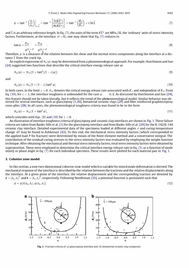
An illustration of interface toughness criteria of glass/epoxy and ceramic clay interfaces are shown in Fig. 1. These failure

criteria are taken from Banks-Sills et al. [1] for the glass/epoxy interface and from Banks-Sills et al. [29] for the K-142/K-144

ceramic clay interface. Detailed experimental data of the specimens loaded at different angles # and curing temperature

change DT may be found in Ashkenazi [43]. To this end, the mechanical stress intensity factors (which corresponded to

the applied load P for fracture) were determined by means of the finite element method and a conservative integral. The

contribution of the residual curing stresses to the stress intensity factors was evaluated by employing the weight function

technique. After obtaining the mechanical and thermal stress intensity factors, total stress intensity factors were obtained by

superposition. These were employed to determine the critical interface energy release rate in Eq. (5) as a function of modemixity or phase angle in Eq. (7) for each individual specimen. These results were plotted for each material pair in Fig. 1.

3. Cohesive zone model

In this section, a new two-dimensional cohesive zone model which is suitable for mixed mode deformation is derived. The

mechanical response of the interface is described by the relation between the tractions and the relative displacements along

the interface. At a given point of the interface, the relative displacement and the corresponding traction are denoted by

d ¼ ½dn; dsT and t ¼ ½t n; t sT, respectively. Following Needleman [35], a potential function is postulated such that

/ ¼ /½dðdn; dtÞ;wðdn; dtÞ ð12Þ

Fig. 1. Fracture criteria of (a) glass/epoxy interface and (b) bimaterial ceramic clay composite.

Y. Freed, L. Banks-Sills/ Engineering Fracture Mechanics 75 (2008) 4583–4593 4585

7/26/2019 4583-4593


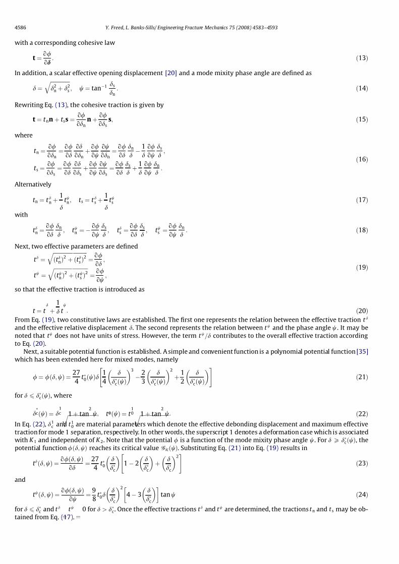
with a corresponding cohesive law

t ¼ o/

od : ð13Þ

In addition, a scalar effective opening displacement [20] and a mode mixity phase angle are defined as

d ¼

ffiffiffiffiffiffiffiffiffiffiffiffiffiffiffid2n

þ d2s

q ; w ¼ tan

1 ds

dn: ð14Þ

Rewriting Eq. (13), the cohesive traction is given by

t ¼ t nn þ t ss ¼ o/

odnn þ

o/

odss; ð15Þ

where

t n ¼ o/

odn¼

o/

od

od

odnþ

o/

ow

ow

odn¼

o/

od

dn

d

1

d

o/

ow

ds

d ;

t s ¼ o/

ods¼

o/

od

od

odsþ

o/

ow

ow

ods¼

o/

od

ds

d þ

1

d

o/

ow

dn

d :

ð16Þ

Alternatively

t n ¼ t dn

þ1

d

t wn; t s ¼ t

ds þ

1

d

t ws

ð17Þ

with

t dn

¼ o/

od

dn

d ; t

wn

¼ o/

ow

ds

d ; t

ds ¼

o/

od

ds

d ; t

ws

¼ o/

ow

dn

d : ð18Þ

Next, two effective parameters are defined

t d ¼

ffiffiffiffiffiffiffiffiffiffiffiffiffiffiffi ffiffiffiffiffiffiffiffiffiffiffiðt d

nÞ2 þ ðt d

sÞ2

q ¼

o/

od ;

t w ¼

ffiffiffiffiffiffiffiffiffiffiffiffiffiffi ffiffiffiffiffiffiffiffiffiffiffiffiðt w

nÞ2 þ ðt w

s Þ2

q ¼

o/

ow;

ð19Þ

so that the effective traction is introduced as

t ¼ t

d

þ

1

d t w

: ð20Þ

From Eq. (19), two constitutive laws are established. The first one represents the relation between the effective traction t d

and the effective relative displacement d. The second represents the relation between t w and the phase angle w . It may be

noted that t w does not have units of stress. However, the term t w=d contributes to the overall effective traction according

to Eq. (20).

Next, a suitable potential function is established. A simple and convenient function is a polynomial potential function [35]

which has been extended here for mixed modes, namely

/ ¼ /ðd;wÞ ¼ 27

4 t

0

ðwÞd 1

4

d

dcðwÞ

3

2

3

d

dcðwÞ

2

þ1

2

d

dcðwÞ

" # ð21Þ

for d 6 dcðwÞ, where

dcðwÞ ¼ d

1

c ffiffiffiffiffiffiffiffiffiffiffiffiffiffiffiffi ffiffiffiffiffiffi1 þ tan2

wq ; t 0ðwÞ ¼ t 1

0 ffiffiffiffiffiffiffiffiffiffiffiffiffiffiffi ffiffiffiffiffiffiffi1 þ tan2

wq : ð22Þ

In Eq. (22), d1c and t 10 are material parameters which denote the effective debonding displacement and maximum effective

traction for mode 1 separation, respectively. In other words, the superscript 1 denotes a deformation case which is associated

with K 1 and independent of K 2. Note that the potential / is a function of the mode mixity phase angle w. For d P dcðwÞ, the

potential function /ðd;wÞ reaches its critical value GicðwÞ. Substituting Eq. (21) into Eq. (19) results in

t dðd;wÞ ¼

o/ðd;wÞ

od ¼

27

4 t

0

d

dc

1 2

d

dc

þ

d

dc

2" #

ð23Þ

and

t wðd;wÞ ¼

o/ðd;wÞ

ow ¼

9

8t

0d d

dc

2

4 3 d

dc

tanw ð24Þ

for d 6 dc and t d

¼ t w

¼ 0 for d > d

c. Once the effective tractions t d and t w are determined, the tractions t n and t s may be ob-

tained from Eq. (17).


7/26/2019 4583-4593


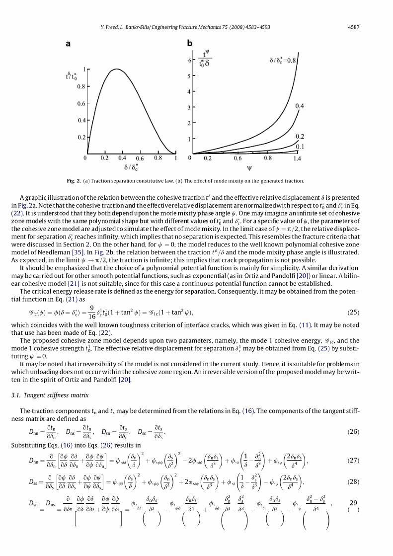
A graphic illustration of the relation between the cohesive traction t d and the effective relative displacement d is presented

in Fig. 2a. Note that the cohesive traction and the effectiverelative displacement are normalizedwith respect to t 0 and dc in Eq.

(22). It is understood that they both depend upon the mode mixity phase angle w. One may imagine an infinite set of cohesive

zone models with the same polynomial shape but with different values of t 0 and dc. For a specific value of w, the parameters of

the cohesive zone model are adjusted to simulate the effect of mode mixity. In the limit case of w ¼ p=2, the relative displace-

ment for separation dc reaches infinity, which implies that no separation is expected. This resembles the fracture criteria that

were discussed in Section 2. On the other hand, for w ¼ 0, the model reduces to the well known polynomial cohesive zone

model of Needleman [35]. In Fig. 2b, the relation between the traction t w=d and the mode mixity phase angle is illustrated.

As expected, in the limit w ! p=2, the traction is infinite; this implies that crack propagation is not possible.

It should be emphasized that the choice of a polynomial potential function is mainly for simplicity. A similar derivation

may be carried out for other smooth potential functions, such as exponential (as in Ortiz and Pandolfi [20]) or linear. A bilin-

ear cohesive model [21] is not suitable, since for this case a continuous potential function cannot be established.

The critical energy release rate is defined as the energy for separation. Consequently, it may be obtained from the poten-

tial function in Eq. (21) as

GicðwÞ ¼ /ðd ¼ dcÞ ¼

9

16d1ct 1

0ð1 þ tan2 wÞ ¼ G1cð1 þ tan2 wÞ; ð25Þ

which coincides with the well known toughness criterion of interface cracks, which was given in Eq. (11). It may be noted

that use has been made of Eq. (22).

The proposed cohesive zone model depends upon two parameters, namely, the mode 1 cohesive energy, G1c, and the

mode 1 cohesive strength t 10. The effective relative displacement for separation d1c may be obtained from Eq. (25) by substi-

tuting w ¼ 0.

It may be noted that irreversibility of the model is not considered in the current study. Hence, it is suitable for problems in

which unloading does not occur within the cohesive zone region. An irreversible version of the proposed model may be writ-

ten in the spirit of Ortiz and Pandolfi [20].

3.1. Tangent stiffness matrix

The traction components t n and t s may be determined from the relations in Eq. (16). The components of the tangent stiff-

ness matrix are defined as

Dnn ¼ ot n

odn; Dns ¼

ot n

ods; Dsn ¼

ot s

odn; Dss ¼

ot s

ods: ð26Þ

Substituting Eqs. (16) into Eqs. (26) results in

Dnn ¼ o

odn

o/

od

od

odnþ

o/

ow

ow

odn

¼ /;dd

dn

d

2

þ /;wwds

d2

2

2/;dwdnds

d3

þ /;d

1

d d2

n

d3

!þ /;w

2dnds

d4

; ð27Þ

Dss ¼ o

ods

o/

od

od

odsþ

o/

ow

ow

ods

¼ /;dd

ds

d

2

þ /;wwdn

d2

2

þ 2/;dwdnds

d3

þ /;d

1

d d2

s

d3

! /;w

2dnds

d4

; ð28Þ

Dsn

¼ Dns

¼

o

odn

o/

od

od

ods þ

o/

ow

ow

ods ¼ /;

dd

dnds

d2 /;

ww

dnds

d4 þ /;

dw

d2n

d3

d2s

d3 ! /;

d

dnds

d3 /;

w

d2n

d2s

d4 !; ð

29Þ

Fig. 2. (a) Traction separation constitutive law. (b) The effect of mode mixity on the generated traction.


http://-/?-

http://-/?-

7/26/2019 4583-4593


where

/;d ¼ t d ¼

27

4 t

0

d

dc

1 2

d

dc

þ

d

dc

2" #

; ð30Þ

/;dd ¼ 27

4

t 0

dc

1 4 d

dc

þ 3

d

dc

2" #

; ð31Þ

/;dw ¼ 27

2 t 0 dd

c

3

d

c dd tanw; ð32Þ

/;w ¼ t w ¼

9

8t

0

d

dc

2

4 3 d

dc

d tanw; ð33Þ

/;ww ¼ 9

8t

0

d

dc

3

4dc 3d 1 tan

2 w

: ð34Þ

If d > dc, then Dnn ¼ Dss ¼ Dns ¼ Dsn ¼ 0.

3.2. Cohesive interface element

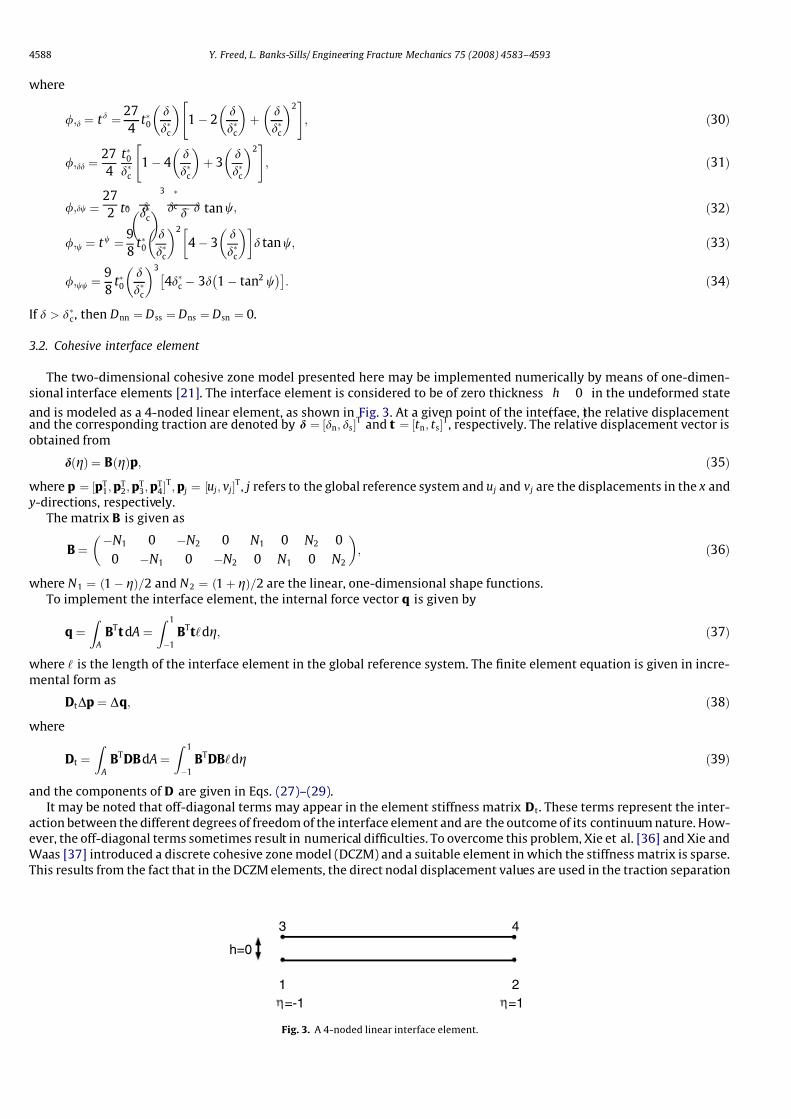
The two-dimensional cohesive zone model presented here may be implemented numerically by means of one-dimen-

sional interface elements [21]. The interface element is considered to be of zero thickness

ðh

¼ 0

Þ in the undeformed state

and is modeled as a 4-noded linear element, as shown in Fig. 3. At a given point of the interface, the relative displacementand the corresponding traction are denoted by d ¼ ½dn; dsT and t ¼ ½t n; t sT, respectively. The relative displacement vector is

obtained from

dðgÞ ¼ BðgÞp; ð35Þ

where p ¼ ½pT1; pT

2; pT3; pT

4T; p j ¼ ½u j; v jT, j refers to the global reference system and u j and v j are the displacements in the x and

y-directions, respectively.

The matrix B is given as

B ¼ N 1 0 N 2 0 N 1 0 N 2 0

0 N 1 0 N 2 0 N 1 0 N 2

; ð36Þ

where N 1 ¼ ð1 gÞ=2 and N 2 ¼ ð1 þ gÞ=2 are the linear, one-dimensional shape functions.

To implement the interface element, the internal force vector q is given by

q ¼Z A

BTtd A ¼

Z 11

BTt‘dg; ð37Þ

where ‘ is the length of the interface element in the global reference system. The finite element equation is given in incre-

mental form as

DtDp ¼ Dq; ð38Þ

where

Dt ¼

Z A

BTDBd A ¼

Z 11

BTDB‘dg ð39Þ

and the components of D are given in Eqs. (27)–(29).

It may be noted that off-diagonal terms may appear in the element stiffness matrix Dt. These terms represent the inter-

action between the different degrees of freedom of the interface element and are the outcome of its continuum nature. How-

ever, the off-diagonal terms sometimes result in numerical difficulties. To overcome this problem, Xie et al. [36] and Xie and

Waas [37] introduced a discrete cohesive zone model (DCZM) and a suitable element in which the stiffness matrix is sparse.

This results from the fact that in the DCZM elements, the direct nodal displacement values are used in the traction separation

1 2

3 4

h=0

=-1 =1

Fig. 3. A 4-noded linear interface element.


7/26/2019 4583-4593


laws, rather than the interpolated values as in the continuum framework used here. The performance of the DCZM frame-

work in conjunction with the new cohesive zone model should be investigated.

4. Implementation and simulation

In this section, the validity of the cohesive zone model is examined and a methodology for obtaining the parameters of the

model is discussed. To this end, the proposed model was implemented as a user supplied material subroutine in the com-

mercial finite element package ABAQUS [38]. First, a double cantilever beam (DCB) specimen was analyzed. The effect of thecohesive strength on the behavior of this specimen was examined. Next, mixed mode deformation was simulated by means

of a Brazilian disk specimen and a new failure criterion is suggested.

4.1. Numerical simulation of double cantilever beam specimen

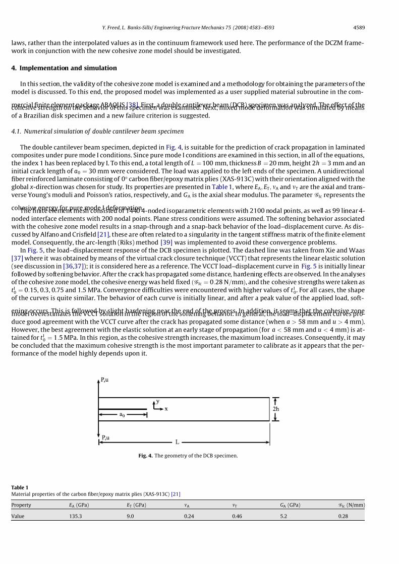
The double cantilever beam specimen, depicted in Fig. 4, is suitable for the prediction of crack propagation in laminated

composites under pure mode I conditions. Since pure mode I conditions are examined in this section, in all of the equations,

the index 1 has been replaced by I. To this end, a total length of L ¼ 100 mm, thickness B ¼ 20 mm, height 2h ¼ 3 mm and an

initial crack length of a0 ¼ 30 mm were considered. The load was applied to the left ends of the specimen. A unidirectional

fiber reinforced laminate consisting of 0 carbon fiber/epoxy matrix plies (XAS-913C) with their orientation aligned with the

global x-direction was chosen for study. Its properties are presented in Table 1, where E A; E T; mA and mT are the axial and trans-

verse Young’s moduli and Poisson’s ratios, respectively, and GA is the axial shear modulus. The parameter GIc represents the

cohesive energy for pure mode I deformation.The finite element mesh consisted of 1440 4-noded isoparametric elements with 2100 nodal points, as well as 99 linear 4-

noded interface elements with 200 nodal points. Plane stress conditions were assumed. The softening behavior associated

with the cohesive zone model results in a snap-through and a snap-back behavior of the load–displacement curve. As dis-

cussed by Alfano and Crisfield [21], these are often related to a singularity in the tangent stiffness matrix of the finite element

model. Consequently, the arc-length (Riks) method [39] was implemented to avoid these convergence problems.

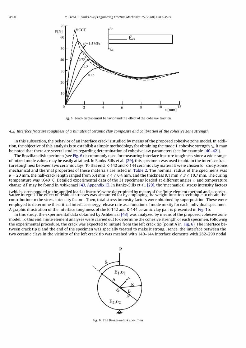
In Fig. 5, the load–displacement response of the DCB specimen is plotted. The dashed line was taken from Xie and Waas

[37] where it was obtained by means of the virtual crack closure technique (VCCT) that represents the linear elastic solution

(see discussion in [36,37]); it is considered here as a reference. The VCCT load–displacement curve in Fig. 5 is initially linear

followed by softening behavior. After the crack has propagated some distance, hardening effects are observed. In the analyses

of the cohesive zone model, the cohesive energy was held fixed ðGIc ¼ 0:28 N=mmÞ, and the cohesive strengths were taken as

t I0 ¼ 0:15, 0.3, 0.75 and 1.5 MPa. Convergence difficulties were encountered with higher values of t I0. For all cases, the shape

of the curves is quite similar. The behavior of each curve is initially linear, and after a peak value of the applied load, soft-

ening occurs. This is followed by slight hardening near the end of the process. In addition, it seems that the cohesive zonemodel overestimates the VCCT solution in the region of the softening behavior. In general, the load–displacement curves pro-

duce good agreement with the VCCT curve after the crack has propagated some distance (when a > 58 mm and u > 4 mm).

However, the best agreement with the elastic solution at an early stage of propagation (for a < 58 mm and u < 4 mm) is at-

tained for t I0 ¼ 1:5 MPa. In this region, as the cohesive strength increases, the maximum load increases. Consequently, it may

be concluded that the maximum cohesive strength is the most important parameter to calibrate as it appears that the per-

formance of the model highly depends upon it.

Fig. 4. The geometry of the DCB specimen.

Table 1

Material properties of the carbon fiber/epoxy matrix plies (XAS-913C) [21]

Property E A (GPa) E T (GPa) mA mT GA (GPa) GIc (N/mm)

Value 135.3 9.0 0.24 0.46 5.2 0.28


7/26/2019 4583-4593


4.2. Interface fracture toughness of a bimaterial ceramic clay composite and calibration of the cohesive zone strength

In this subsection, the behavior of an interface crack is studied by means of the proposed cohesive zone model. In addi-

tion, the objective of this analysis is to establish a simple methodology for obtaining the mode 1 cohesive strength t 10. It may

be noted that there are several studies regarding determination of cohesive law parameters (see for example [40–42]).

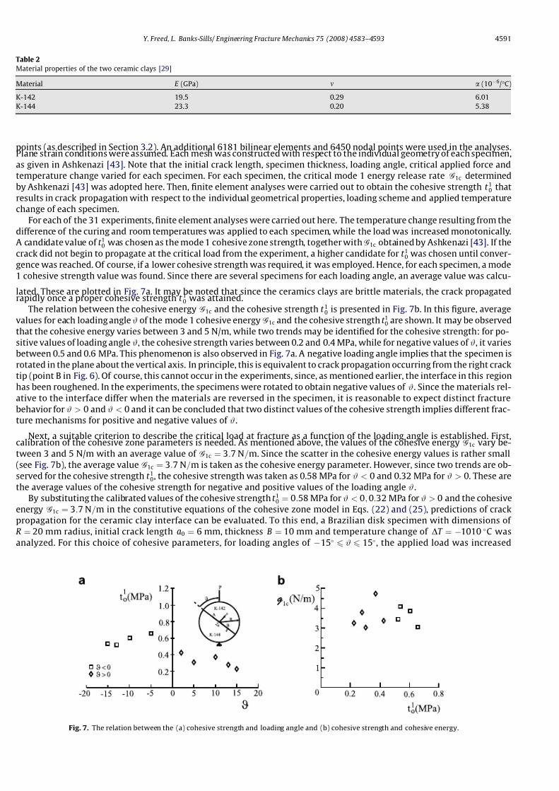
The Brazilian disk specimen (see Fig. 6) is commonly used for measuring interface fracture toughness since a wide range

of mixed mode values may be easily attained. In Banks-Sills et al. [29], this specimen was used to obtain the interface frac-

ture toughness between two ceramic clays. To this end, K-142 and K-144 ceramic clay materials were chosen for study. Some

mechanical and thermal properties of these materials are listed in Table 2. The nominal radius of the specimens was

R ¼ 20 mm, the half-crack length ranged from 5.4 mm 6 a 6 6.4 mm, and the thickness 9.1 mm 6 B 6 10.7 mm. The curing

temperature was 1040 C. Detailed experimental data of the 31 specimens loaded at different angles # and temperature

change DT may be found in Ashkenazi [43, Appendix K]. In Banks-Sills et al. [29], the ‘mechanical’ stress intensity factors

(which corresponded to the applied load at fracture) were determined by means of the finite element method and a conser-vative integral. The effect of residual stresses was accounted for by employing the weight function technique to obtain the

contribution to the stress intensity factors. Then, total stress intensity factors were obtained by superposition. These were

employed to determine the critical interface energy release rate as a function of mode mixity for each individual specimen.

A graphic illustration of the interface toughness of the K-142 and K-144 ceramic clay pair is presented in Fig. 1b.

In this study, the experimental data obtained by Ashkenazi [43] was analyzed by means of the proposed cohesive zone

model. To this end, finite element analyses were carried out to determine the cohesive strength of each specimen. Following

the experimental procedure, the crack was expected to initiate from the left crack tip (point A in Fig. 6). The interface be-

tween crack tip B and the end of the specimen was specially treated to make it strong. Hence, the interface between the

two ceramic clays in the vicinity of the left crack tip was meshed with 140–144 interface elements with 282–290 nodal

Fig. 5. Load–displacement behavior and the effect of the cohesive traction.

Fig. 6. The Brazilian disk specimen.


7/26/2019 4583-4593


points (as described in Section 3.2). An additional 6181 bilinear elements and 6450 nodal points were used in the analyses.Plane strain conditions were assumed. Each mesh was constructed with respect to the individual geometry of each specimen,

as given in Ashkenazi [43]. Note that the initial crack length, specimen thickness, loading angle, critical applied force and

temperature change varied for each specimen. For each specimen, the critical mode 1 energy release rate G1c determined

by Ashkenazi [43] was adopted here. Then, finite element analyses were carried out to obtain the cohesive strength t 10 that

results in crack propagation with respect to the individual geometrical properties, loading scheme and applied temperature

change of each specimen.

For each of the 31 experiments, finite element analyses were carried out here. The temperature change resulting from the

difference of the curing and room temperatures was applied to each specimen, while the load was increased monotonically.

A candidate value of t 10 was chosen as the mode 1 cohesive zone strength, together withG1c obtained by Ashkenazi [43]. If the

crack did not begin to propagate at the critical load from the experiment, a higher candidate for t 10 was chosen until conver-

gence was reached. Of course, if a lower cohesive strength was required, it was employed. Hence, for each specimen, a mode

1 cohesive strength value was found. Since there are several specimens for each loading angle, an average value was calcu-

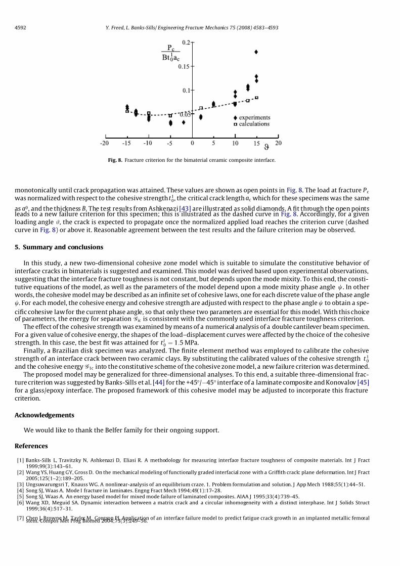
lated. These are plotted in Fig. 7a. It may be noted that since the ceramics clays are brittle materials, the crack propagatedrapidly once a proper cohesive strength t 10 was attained.

The relation between the cohesive energy G1c and the cohesive strength t 10 is presented in Fig. 7b. In this figure, average

values for each loading angle # of the mode 1 cohesive energy G1c and the cohesive strength t 10 are shown. It may be observed

that the cohesive energy varies between 3 and 5 N/m, while two trends may be identified for the cohesive strength: for po-

sitive values of loading angle #, the cohesive strength varies between 0.2 and 0.4 MPa, while for negative values of #, it varies

between 0.5 and 0.6 MPa. This phenomenon is also observed in Fig. 7a. A negative loading angle implies that the specimen is

rotated in the plane about the vertical axis. In principle, this is equivalent to crack propagation occurring from the right crack

tip (point B in Fig. 6). Of course, this cannot occur in the experiments, since, as mentioned earlier, the interface in this region

has been roughened. In the experiments, the specimens were rotated to obtain negative values of #. Since the materials rel-

ative to the interface differ when the materials are reversed in the specimen, it is reasonable to expect distinct fracture

behavior for # > 0 and # < 0 and it can be concluded that two distinct values of the cohesive strength implies different frac-

ture mechanisms for positive and negative values of #.

Next, a suitable criterion to describe the critical load at fracture as a function of the loading angle is established. First,calibration of the cohesive zone parameters is needed. As mentioned above, the values of the cohesive energy G1c vary be-

tween 3 and 5 N/m with an average value of G1c ¼ 3:7 N=m. Since the scatter in the cohesive energy values is rather small

(see Fig. 7b), the average value G1c ¼ 3:7 N=m is taken as the cohesive energy parameter. However, since two trends are ob-

served for the cohesive strength t 10, the cohesive strength was taken as 0.58 MPa for # < 0 and 0.32 MPa for # > 0. These are

the average values of the cohesive strength for negative and positive values of the loading angle #.

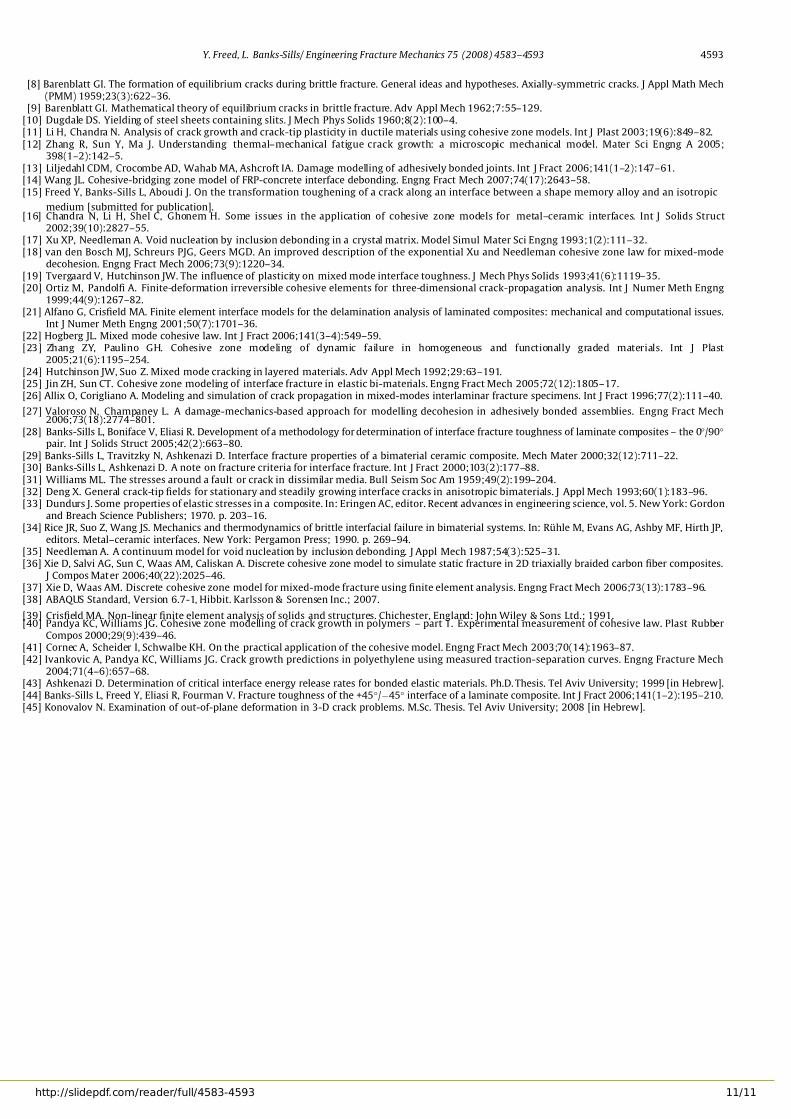
By substituting the calibrated values of the cohesive strength t 10 ¼ 0:58 MPa for # < 0; 0:32 MPa for # > 0 and the cohesive

energy G1c ¼ 3:7 N=m in the constitutive equations of the cohesive zone model in Eqs. (22) and (25), predictions of crack

propagation for the ceramic clay interface can be evaluated. To this end, a Brazilian disk specimen with dimensions of

R ¼ 20 mm radius, initial crack length a0 ¼ 6 mm, thickness B ¼ 10 mm and temperature change of DT ¼ 1010 C was

analyzed. For this choice of cohesive parameters, for loading angles of 15 6 # 6 15 , the applied load was increased

Table 2

Material properties of the two ceramic clays [29]

Material E (GPa) m a (106/C)

K-142 19.5 0.29 6.01

K-144 23.3 0.20 5.38

Fig. 7. The relation between the (a) cohesive strength and loading angle and (b) cohesive strength and cohesive energy.


http://-/?-

http://-/?-

7/26/2019 4583-4593


monotonically until crack propagation was attained. These values are shown as open points in Fig. 8. The load at fracture P cwas normalized with respect to the cohesive strength t 10, the critical crack length ac which for these specimens was the same

as a0, and the thickness B. The test results from Ashkenazi [43] are illustrated as solid diamonds. A fit through the open pointsleads to a new failure criterion for this specimen; this is illustrated as the dashed curve in Fig. 8. Accordingly, for a given

loading angle #, the crack is expected to propagate once the normalized applied load reaches the criterion curve (dashed

curve in Fig. 8) or above it. Reasonable agreement between the test results and the failure criterion may be observed.

5. Summary and conclusions

In this study, a new two-dimensional cohesive zone model which is suitable to simulate the constitutive behavior of

interface cracks in bimaterials is suggested and examined. This model was derived based upon experimental observations,

suggesting that the interface fracture toughness is not constant, but depends upon the mode mixity. To this end, the consti-

tutive equations of the model, as well as the parameters of the model depend upon a mode mixity phase angle w. In other

words, the cohesive model may be described as an infinite set of cohesive laws, one for each discrete value of the phase angle

w. For each model, the cohesive energy and cohesive strength are adjusted with respect to the phase angle w to obtain a spe-

cific cohesive law for the current phase angle, so that only these two parameters are essential for this model. With this choiceof parameters, the energy for separation Gic is consistent with the commonly used interface fracture toughness criterion.

The effect of the cohesive strength was examined by means of a numerical analysis of a double cantilever beam specimen.

For a given value of cohesive energy, the shapes of the load–displacement curves were affected by the choice of the cohesive

strength. In this case, the best fit was attained for t I 0 ¼ 1:5 MPa.

Finally, a Brazilian disk specimen was analyzed. The finite element method was employed to calibrate the cohesive

strength of an interface crack between two ceramic clays. By substituting the calibrated values of the cohesive strength t 10and the cohesive energy G1c into the constitutive scheme of the cohesive zone model, a new failure criterion was determined.

The proposed model may be generalized for three-dimensional analyses. To this end, a suitable three-dimensional frac-

ture criterion was suggested by Banks-Sills et al. [44] for the +45/45 interface of a laminate composite and Konovalov [45]

for a glass/epoxy interface. The proposed framework of this cohesive model may be adjusted to incorporate this fracture

criterion.

Acknowledgements

We would like to thank the Belfer family for their ongoing support.

References

[1] Banks-Sills L, Travitzky N, Ashkenazi D, Eliasi R. A methodology for measuring interface fracture toughness of composite materials. Int J Fract1999;99(3):143–61.

[2] Wang YS, Huang GY, Gross D. On the mechanical modeling of functionally graded interfacial zone with a Griffith crack: plane deformation. Int J Fract2005;125(1–2):189–205.

[3] Ungsuwarungsri T, Knauss WG. A nonlinear-analysis of an equilibrium craze. 1. Problem formulation and solution. J App Mech 1988;55(1):44–51.[4] Song SJ, Waas A. Mode I fracture in laminates. Engng Fract Mech 1994;49(1):17–28.[5] Song SJ, Waas A. An energy based model for mixed mode failure of laminated composites. AIAA J 1995;33(4):739–45.[6] Wang XD, Meguid SA. Dynamic interaction between a matrix crack and a circular inhomogeneity with a distinct interphase. Int J Solids Struct

1999;36(4):517–31.

[7] Chen J, Browne M, Taylor M, Gregson PJ. Application of an interface failure model to predict fatigue crack growth in an implanted metallic femoralstem. Compos Met Prog Biomed 2004;73(3):249–56.

Fig. 8. Fracture criterion for the bimaterial ceramic composite interface.


7/26/2019 4583-4593


[8] Barenblatt GI. The formation of equilibrium cracks during brittle fracture. General ideas and hypotheses. Axially-symmetric cracks. J Appl Math Mech(PMM) 1959;23(3):622–36.

[9] Barenblatt GI. Mathematical theory of equilibrium cracks in brittle fracture. Adv Appl Mech 1962;7:55–129.[10] Dugdale DS. Yielding of steel sheets containing slits. J Mech Phys Solids 1960;8(2):100–4.[11] Li H, Chandra N. Analysis of crack growth and crack-tip plasticity in ductile materials using cohesive zone models. Int J Plast 2003;19(6):849–82.[12] Zhang R, Sun Y, Ma J. Understanding thermal–mechanical fatigue crack growth: a microscopic mechanical model. Mater Sci Engng A 2005;

398(1–2):142–5.[13] Liljedahl CDM, Crocombe AD, Wahab MA, Ashcroft IA. Damage modelling of adhesively bonded joints. Int J Fract 2006;141(1–2):147–61.[14] Wang JL. Cohesive-bridging zone model of FRP-concrete interface debonding. Engng Fract Mech 2007;74(17):2643–58.[15] Freed Y, Banks-Sills L, Aboudi J. On the transformation toughening of a crack along an interface between a shape memory alloy and an isotropic

medium [submitted for publication].[16] Chandra N, Li H, Shel C, Ghonem H. Some issues in the application of cohesive zone models for metal–ceramic interfaces. Int J Solids Struct

2002;39(10):2827–55.[17] Xu XP, Needleman A. Void nucleation by inclusion debonding in a crystal matrix. Model Simul Mater Sci Engng 1993;1(2):111–32.[18] van den Bosch MJ, Schreurs PJG, Geers MGD. An improved description of the exponential Xu and Needleman cohesive zone law for mixed-mode

decohesion. Engng Fract Mech 2006;73(9):1220–34.[19] Tvergaard V, Hutchinson JW. The influence of plasticity on mixed mode interface toughness. J Mech Phys Solids 1993;41(6):1119–35.[20] Ortiz M, Pandolfi A. Finite-deformation irreversible cohesive elements for three-dimensional crack-propagation analysis. Int J Numer Meth Engng

1999;44(9):1267–82.[21] Alfano G, Crisfield MA. Finite element interface models for the delamination analysis of laminated composites: mechanical and computational issues.

Int J Numer Meth Engng 2001;50(7):1701–36.[22] Hogberg JL. Mixed mode cohesive law. Int J Fract 2006;141(3–4):549–59.[23] Zhang ZY, Paulino GH. Cohesive zone modeling of dynamic failure in homogeneous and functionally graded materials. Int J Plast

2005;21(6):1195–254.[24] Hutchinson JW, Suo Z. Mixed mode cracking in layered materials. Adv Appl Mech 1992;29:63–191.[25] Jin ZH, Sun CT. Cohesive zone modeling of interface fracture in elastic bi-materials. Engng Fract Mech 2005;72(12):1805–17.[26] Allix O, Corigliano A. Modeling and simulation of crack propagation in mixed-modes interlaminar fracture specimens. Int J Fract 1996;77(2):111–40.

[27] Valoroso N, Champaney L. A damage-mechanics-based approach for modelling decohesion in adhesively bonded assemblies. Engng Fract Mech2006;73(18):2774–801.

[28] Banks-Sills L, Boniface V, Eliasi R. Development of a methodology for determination of interface fracture toughness of laminate composites – the 0/90pair. Int J Solids Struct 2005;42(2):663–80.

[29] Banks-Sills L, Travitzky N, Ashkenazi D. Interface fracture properties of a bimaterial ceramic composite. Mech Mater 2000;32(12):711–22.[30] Banks-Sills L, Ashkenazi D. A note on fracture criteria for interface fracture. Int J Fract 2000;103(2):177–88.[31] Williams ML. The stresses around a fault or crack in dissimilar media. Bull Seism Soc Am 1959;49(2):199–204.[32] Deng X. General crack-tip fields for stationary and steadily growing interface cracks in anisotropic bimaterials. J Appl Mech 1993;60(1):183–96.[33] Dundurs J. Some properties of elastic stresses in a composite. In: Eringen AC, editor. Recent advances in engineering science, vol. 5. New York: Gordon

and Breach Science Publishers; 1970. p. 203–16.[34] Rice JR, Suo Z, Wang JS. Mechanics and thermodynamics of brittle interfacial failure in bimaterial systems. In: Rühle M, Evans AG, Ashby MF, Hirth JP,

editors. Metal–ceramic interfaces. New York: Pergamon Press; 1990. p. 269–94.[35] Needleman A. A continuum model for void nucleation by inclusion debonding. J Appl Mech 1987;54(3):525–31.[36] Xie D, Salvi AG, Sun C, Waas AM, Caliskan A. Discrete cohesive zone model to simulate static fracture in 2D triaxially braided carbon fiber composites.

J Compos Mat er 2006;40(22):2025–46.[37] Xie D, Waas AM. Discrete cohesive zone model for mixed-mode fracture using finite element analysis. Engng Fract Mech 2006;73(13):1783–96.[38] ABAQUS Standard, Version 6.7-1, Hibbit. Karlsson & Sorensen Inc.; 2007.

[39] Crisfield MA. Non-linear finite element analysis of solids and structures. Chichester, England: John Wiley & Sons Ltd.; 1991.[40] Pandya KC, Williams JG. Cohesive zone modelling of crack growth in polymers – part 1. Experimental measurement of cohesive law. Plast Rubber

Compos 2000;29(9):439–46.[41] Cornec A, Scheider I, Schwalbe KH. On the practical application of the cohesive model. Engng Fract Mech 2003;70(14):1963–87.[42] Ivankovic A, Pandya KC, Williams JG. Crack growth predictions in polyethylene using measured traction-separation curves. Engng Fracture Mech

2004;71(4–6):657–68.[43] Ashkenazi D. Determination of critical interface energy release rates for bonded elastic materials. Ph.D. Thesis. Tel Aviv University; 1999 [in Hebrew].[44] Banks-Sills L, Freed Y, Eliasi R, Fourman V. Fracture toughness of the +45/45 interface of a laminate composite. Int J Fract 2006;141(1–2):195–210.[45] Konovalov N. Examination of out-of-plane deformation in 3-D crack problems. M.Sc. Thesis. Tel Aviv University; 2008 [in Hebrew].


Documents

4583-4593