Embed Size (px)
Citation preview
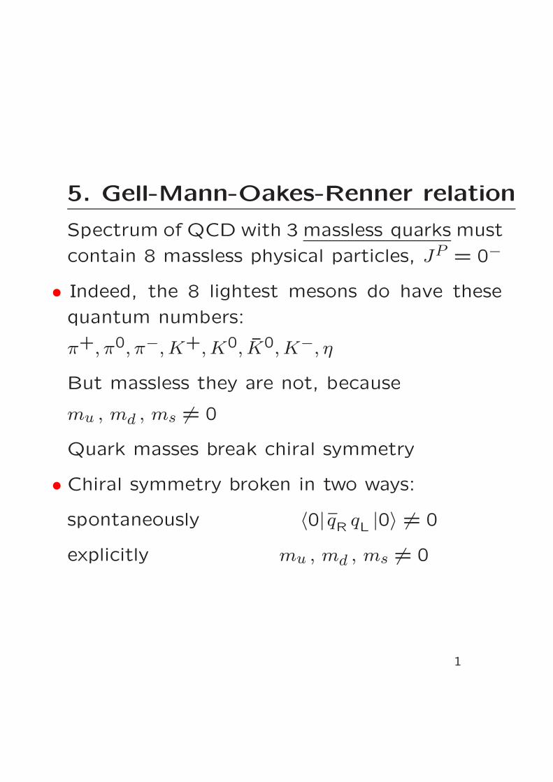
5. Gell-Mann-Oakes-Renner relation
Spectrum of QCD with 3 massless quarks must
contain 8 massless physical particles, JP = 0−
• Indeed, the 8 lightest mesons do have these
quantum numbers:
π+, π0, π−,K+,K0, K0,K−, η
But massless they are not, because
mu , md , ms 6= 0
Quark masses break chiral symmetry
• Chiral symmetry broken in two ways:
spontaneously 〈0|qR qL |0〉 6= 0
explicitly mu , md , ms 6= 0
1
• HQCD only has approximate symmetry, to the
extent that mu,md,ms are small
HQCD = H0 +H1
H1 =
∫
d3x muuu+mddd+msss
• H0 is Hamiltonian of the massless theory,
invariant under SU(3)R×SU(3)L
• H1 breaks the symmetry,
transforms with (3, 3) ⊕ (3,3)
• For the low energy structure of QCD, the
heavy quarks do not play an essential role:
c, b, t are singlets under SU(3)R×SU(3)L
Can include the heavy quarks in H0
• Nambu-Goldstone bosons are massless only if
the symmetry is exact
2
Gell-Mann-Oakes-Renner formula:
M2π = (mu +md) × |〈0|uu |0〉| × 1
F2π
1968
⇑ ⇑explicit spontaneous
Coefficient: decay constant Fπ
• Why M2π ∝ (mu +md) ?
〈0|u(x)γµγ5d(x)|π−〉=i√
2Fπ pµe−ip·x
〈0|u(x) i γ5d(x)|π−〉=√
2Gπe−ip·x
• Current conservation
∂µ(uγµγ5d)=(mu +md)u i γ5d
⇒√
2Fπ p2=(mu +md)
√2Gπ
p2=M2π
⇒ M2π = (mu +md)
Gπ
Fπexact
• Expand in powers of mu,md:
Gπ
Fπ= B +O(m)
⇒M2π = (mu +md)B +O(m2)
3
•M2π = (mu +md)B +O(m2)
•Mπ disappears if the symmetry breaking
is turned off, mu,md → 0√
• Explains why the pseudoscalar mesons
have very different masses
M2K+ = (mu +ms)B +O(m2)
M2K− = (md +ms)B +O(m2)
⇒M2K is about 13 times larger than M2
π , because
mu,md happen to be small compared to ms
• First order perturbation theory also yields
M2η = 1
3 (mu +md + 4ms)B +O(m2)
⇒M2π − 4M2
K + 3M2η = O(m2)
Gell-Mann-Okubo formula for M2√
4
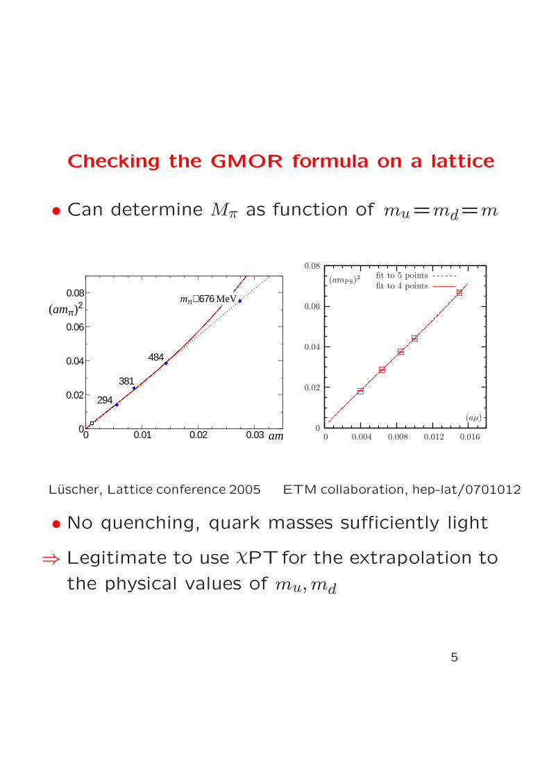
Checking the GMOR formula on a lattice
• Can determine Mπ as function of mu=md=m
0 0.01 0.02 0.03am0
0.02
0.04
0.06
0.08
(amπ)2mπ∼676 MeV
484
381
294
fit to 4 pointsfit to 5 points
(amPS)2
(aµ)
0.0160.0120.0080.0040
0.08
0.06
0.04
0.02
0
Luscher, Lattice conference 2005 ETM collaboration, hep-lat/0701012
• No quenching, quark masses sufficiently light
⇒ Legitimate to use χPTfor the extrapolation to
the physical values of mu,md
5
• Quality of data is impressive
• Proportionality of M2π to the quark mass ap-
pears to hold out to values of mu,md that are
an order of magnitude larger than in nature
• Main limitation: systematic uncertainties
in particular: Nf = 2 → Nf = 3
6
II. Chiral perturbation theory
6. Group geometry
• QCD with 3 massless quarks:
spontaneous symmetry breakdown
from SU(3)R×SU(3)L to SU(3)V
generates 8 Nambu-Goldstone bosons
• Generalization: suppose symmetry group
of Hamiltonian is Lie group G
Generators Q1, Q2, . . . , QD, D = dim(G)
For some generators Qi |0〉 6= 0
How many Nambu-Goldstone bosons ?
• Consider those elements of the Lie algebra
Q = α1Q1 + . . .+ αnQD, for which Q |0〉 = 0
These elements form a subalgebra:
Q |0〉 = 0, Q′ |0〉 = 0 ⇒ [Q,Q′] |0〉 = 0
Dimension of subalgebra: d ≤ D
• Of the D vectors Qi |0〉D − d are linearly independent
⇒ D − d different physical states of zero mass⇒ D − d Nambu-Goldstone bosons
7
• Subalgebra generates subgroup H⊂G
H is symmetry group of the ground state
coset space G/H contains as many parameters
as there are Nambu-Goldstone bosons
d = dim(H), D = dim(G)
⇒ Nambu-Goldstone bosons live on the coset
G/H
• Example: QCD with Nf massless quarks
G = SU(Nf)R × SU(Nf)L
H = SU(Nf)V
D = 2(N2f − 1), d = N2
f − 1
N2f − 1 Nambu-Goldstone bosons
• It so happens that mu,md ≪ ms
• mu = md = 0 is an excellent approximation
SU(2)R× SU(2)L is a nearly exact symmetry
Nf = 2, N2f − 1 = 3 Nambu-Goldstone bosons
(pions)
8
7. Generating functional of QCD
• Basic objects for quantitative analysis of QCD:
Green functions of the currents
V µa =q γµ12λa q , A
µa = q γµγ5
12λa q ,
Sa=q 12λa q , Pa = q i γ5
12λa q
Include singlets, with λ0 =√
2/3× 1, as well as
ω =1
16π2trcGµνG
µν
• Can collect all of the Green functions formed
with these operators in a generating functional:
Perturb the system with external fields
vaµ(x), aaµ(x), sa(x), p
a(x), θ(x)
Replace the Lagrangian of the massless theory
L0 = − 1
2g2trcGµνG
µν + q iγµ(∂µ − iGµ) q
by L = L0 + L1
L1 = vaµVµa + aaµA
µa − saSa − paPa − θ ω
• Quark mass terms are included in the external
field sa(x)
9
• |0 in〉: system is in ground state for x0 → −∞Probability amplitude for finding ground state
when x0 → +∞:
eiSQCDv,a,s,p,θ=〈0out|0 in〉v,a,s,p,θ
• Expressed in terms of ground state of L0:
eiSQCDv,a,s,p,θ=〈0|T exp i∫
dxL1 |0〉
• Expansion of SQCDv, a, s, p, θ in powers of the
external fields yields the connected parts of
the Green functions of the massless theory
SQCDv, a, s, p, θ = −∫
dx sa(x)〈0|Sa(x) |0〉
+ i2
∫
dxdy aaµ(x)abν(y)〈0| TAµa(x)Aνb(y) |0〉conn + . . .
• SQCDv, a, s, p, θ is referred to as the
generating functional of QCD
• For Green functions of full QCD, set
sa(x) = ma + sa(x) , ma = trλam
and expand around sa(x) = 0
10
• Path integral representation for generating
functional:
eiSQCDv,a,s,p = N∫
[dG] e i∫
dxLG detD
LG = − 1
2g2trcGµνG
µν − θ
16π2trcGµνG
µν
D = iγµ∂µ − i(Gµ + vµ + aµγ5) − s− iγ5p
Gµ is matrix in colour space
vµ, aµ, s, p are matrices in flavour space
vµ(x) ≡ 12λa v
aµ(x), etc.
11
8. Ward identities
Symmetry in terms of Green functions
• Lagrangian is invariant under
qR(x) → VR(x) qR(x) , qL(x) → VL(x) qL(x)
VR(x), VL(x) ∈ U(3)
provided the external fields are transformed with
v′µ + a′µ=VR(vµ + aµ)V†R − i∂µVRV
†R
v′µ − a′µ=VL(vµ − aµ)V†L − i∂µVLV
†L
s′ + i p′=VR(s+ i p)V†L
The operation takes the Dirac operator into
D′=
P−VR + P+VL
D
P+V†R + P−V
†L
P±=12(1 ± γ5)
• detD requires regularization
∃/ symmetric regularization
⇒ detD′ 6= detD, only |detD′ | = |detD |symmetry does not survive quantization
12
• Change in detD can explicitly be calculated
For an infinitesimal transformation
VR = 1+ i α+ iβ+ . . . , VL = 1+ i α− iβ+ . . .
the change in the determinant is given by
detD′ = detD e−i∫
dx 2〈β〉ω+〈βΩ〉
〈A〉 ≡ trA
ω =1
16π2trcGµνG
µν gluons
Ω =Nc
4π2ǫµνρσ∂µvν∂ρvσ + . . . ext. fields
• Consequence for generating functional:
The term with ω amounts to a change in θ,
can be compensated by θ′ = θ − 2 〈β〉Pull term with 〈βΩ〉 outside the path integral
⇒ SQCDv′, a′, s′, p′, θ′ = SQCDv, a, s, p, θ −∫
dx〈βΩ〉
13
SQCDv′, a′, s′, p′, θ′ = SQCDv, a, s, p, θ −∫
dx〈βΩ〉
• SQCD is invariant under U(3)R×U(3)L, except
for a specific change due to the anomalies
• Relation plays key role in low energy analysis:
collects all of the Ward identities
For the octet part of the axial current,e.g.
∂xµ〈0|TAµa(x)Pb(y) |0〉 = −14 i δ(x− y)〈0|qλa, λbq |0〉
+ 〈0|Tq(x) iγ5m, 12λaq(x)Pb(y) |0〉
• Symmetry of the generating functional implies
the operator relations
∂µVµa =q i[m, 12λa]q , a = 0, . . . ,8
∂µAµa=q iγ5m, 12λaq , a = 1, . . . ,8
∂µAµ0 =
√
23 q iγ5mq+
√6ω
• Textbook derivation of the Ward identities
goes in inverse direction, but is slippery
formal manipulations, anomalies ?
14
9. Low energy expansion
• If the spectrum has an energy gap
⇒ no singularities in scattering amplitudes
or Green functions near p = 0
⇒ low energy behaviour may be analyzed with
Taylor series expansion in powers of p
f(t)=1 + 16〈r
2〉 t+ . . . form factor
T(p)=a+ b p2 + . . . scattering amplitude
Cross section dominated by
S–wave scattering length
dσ
dΩ≃ |a|2
• Expansion parameter:p
m=
momentum
energy gap
• Taylor series only works if the spectrum
has an energy gap, i.e. if there are
no massless particles
15
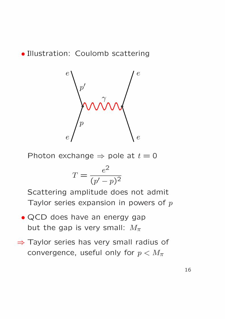
• Illustration: Coulomb scattering
p
p′
e
e
e
e
γ
Photon exchange ⇒ pole at t = 0
T =e2
(p′ − p)2
Scattering amplitude does not admit
Taylor series expansion in powers of p
• QCD does have an energy gap
but the gap is very small: Mπ
⇒ Taylor series has very small radius of
convergence, useful only for p < Mπ
16
• Massless QCD contains infrared singularities
due to the Nambu-Goldstone bosons
• For mu = md = 0, pion exchange gives rise to
poles and branch points at p = 0
⇒ Low energy expansion is not a Taylor series,
contains logarithms
Singularities due to Nambu-Goldstone bosons can
be worked out with an effective field theory
Chiral Perturbation Theory
Weinberg, Dashen, Pagels, Gasser, . . .
• Chiral perturbation theory correctly reproduces
the infrared singularities of QCD
• Quantities of interest are expanded in powers
of external momenta and quark masses
• Expansion has been worked out to
next-to-leading order for many quantities
”Chiral perturbation theory to one loop”
• In quite a few cases, the next-to-next-to-leading
order is also known
17
• Properties of the Nambu-Goldstone bosons are
governed by the hidden symmetry that
is responsible for their occurrence
• Focus on the singularities due to the pions
HQCD = H0 +H1
H1 =∫
d3x muuu+mddd
H0 is invariant under G = SU(2)R × SU(2)L
|0〉 is invariant under H = SU(2)V
mass term of strange quark is included in H0
• Treat H1 as a perturbation
Expansion in
powers of H1
⇐⇒ Expansion in
powers of mu,md
• Extension to SU(3)R×SU(3)L straightforward:
include singularities due to exchange of K, η
18
10. Effective Lagrangian
• Replace quarks and gluons by pions
~π(x) = π1(x), π2(x), π3(x)LQCD → Leff
• Central claim:
A. Effective theory yields alternative
representation for generating functional of QCD
eiSQCDv,a,s,p,θ = Neff
∫
[dπ]ei∫
dxLeff~π,v,a,s,p,θ
B. Leff has the same symmetries as LQCD
⇒ Can calculate the low energy expansion of the
Green functions with the effective theory.
If Leff is chosen properly, this reproduces the
low energy expansion of QCD, order by order.
• Proof of A and B: H.L., Annals Phys. 1994
19
• Pions live on the coset G/H = SU(2)
~π(x) → U(x) ∈ SU(2)
The fields ~π(x) are the coordinates of U(x)
Can use canonical coordinates, for instance
U = exp i ~π · ~τ ∈ SU(2)
• Action of the symmetry group on the quarks:
q′R = VR · qR , q′L = VL · qL
• Action on the pion field:
U ′ = VR · U · V †L
Note: Transformation law for the coordinates
~π is complicated, nonlinear
• Except for the contribution from the
anomalies, Leff is invariant
LeffU ′, v′, a′, s′, p′, θ′ = LeffU, v, a, s, p, θ
Symmetry of SQCD implies symmetry of Leff20
11. Explicit construction of Leff
• First ignore the external fields,
Leff = Leff(U, ∂U, ∂2U, . . .)
Derivative expansion:
Leff = f0(U)+f1(U)× U+f2(U)×∂µU×∂µU+. . .⇑ ⇑ ⇑O(1) O(p2) O(p2)
Amounts to expansion in powers of momenta
• Term of O(1): f0(U) = f0(VRUV†L )
VR = 1 , VL = U → VRUV†L = 1
⇒ f0(U) = f0(1) irrelevant constant, drop it
• Term with U : integrate by parts
⇒ can absorb f1(U) in f2(U)
21
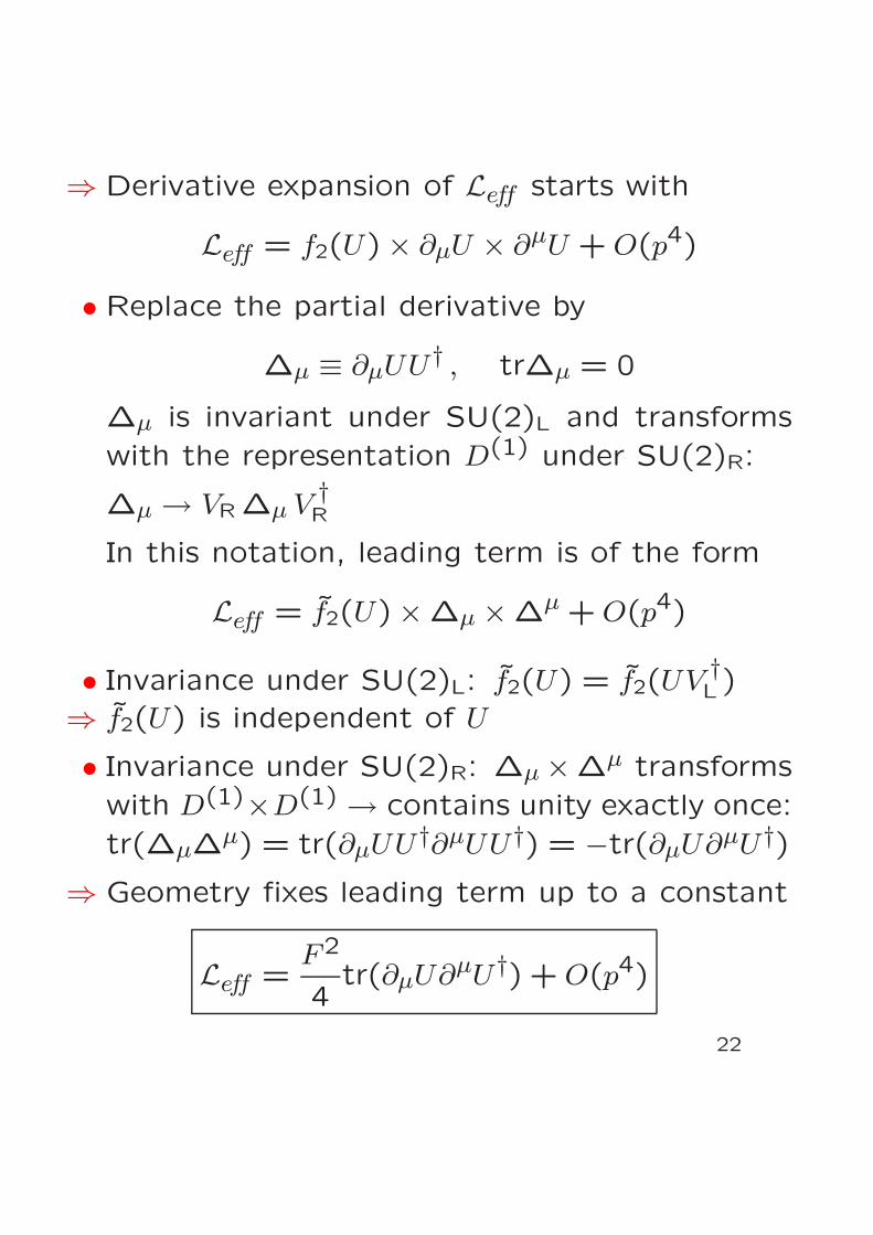
⇒ Derivative expansion of Leff starts with
Leff = f2(U) × ∂µU × ∂µU +O(p4)
• Replace the partial derivative by
∆µ ≡ ∂µUU† , tr∆µ = 0
∆µ is invariant under SU(2)L and transforms
with the representation D(1) under SU(2)R:
∆µ → VR ∆µ V†R
In this notation, leading term is of the form
Leff = f2(U) × ∆µ × ∆µ +O(p4)
• Invariance under SU(2)L: f2(U) = f2(UV†L )
⇒ f2(U) is independent of U
• Invariance under SU(2)R: ∆µ×∆µ transforms
with D(1)×D(1) → contains unity exactly once:
tr(∆µ∆µ) = tr(∂µUU†∂µUU†) = −tr(∂µU∂µU†)
⇒ Geometry fixes leading term up to a constant
Leff =F2
4tr(∂µU∂
µU†) +O(p4)
22
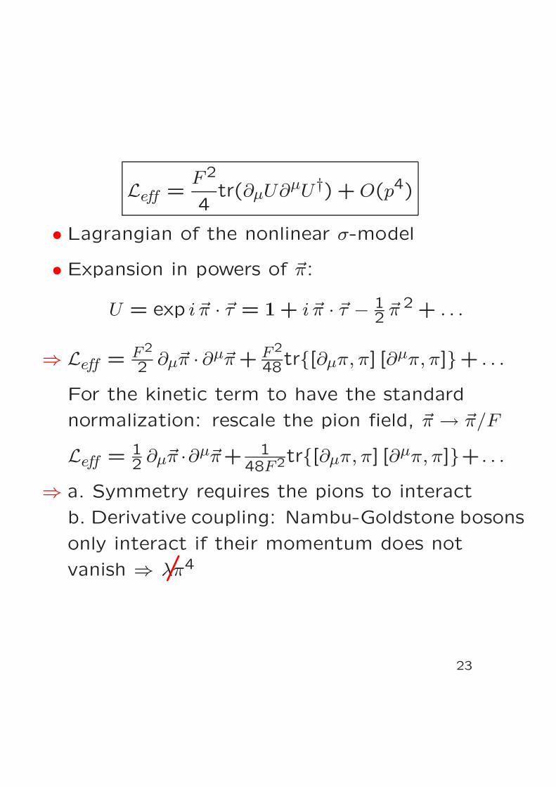
Leff =F2
4tr(∂µU∂
µU†) +O(p4)
• Lagrangian of the nonlinear σ-model
• Expansion in powers of ~π:
U = exp i ~π · ~τ = 1 + i ~π · ~τ − 12 ~π
2 + . . .
⇒ Leff = F2
2 ∂µ~π · ∂µ~π+ F2
48tr[∂µπ, π] [∂µπ, π]+ . . .
For the kinetic term to have the standard
normalization: rescale the pion field, ~π → ~π/F
Leff = 12 ∂µ~π ·∂µ~π+ 1
48F2tr[∂µπ, π] [∂µπ, π]+ . . .
⇒ a. Symmetry requires the pions to interact
b. Derivative coupling: Nambu-Goldstone bosons
only interact if their momentum does not
vanish ⇒ λπ4/
23
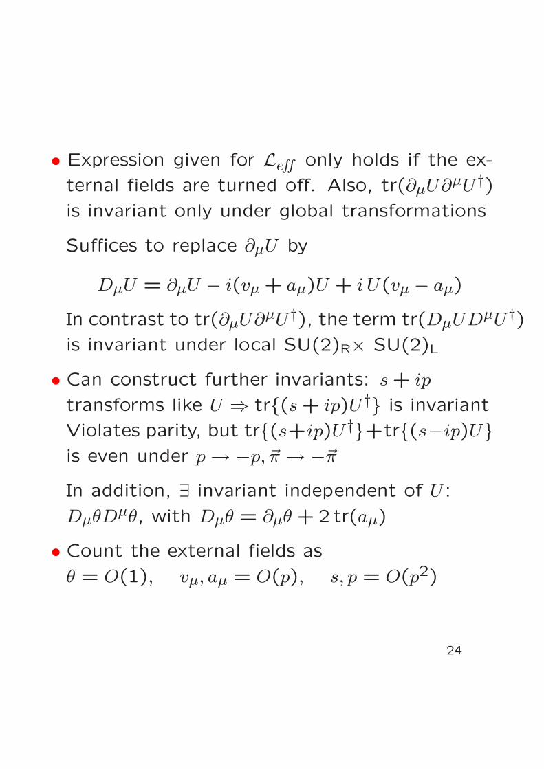
• Expression given for Leff only holds if the ex-
ternal fields are turned off. Also, tr(∂µU∂µU†)is invariant only under global transformations
Suffices to replace ∂µU by
DµU = ∂µU − i(vµ + aµ)U + i U(vµ − aµ)
In contrast to tr(∂µU∂µU†), the term tr(DµUDµU†)is invariant under local SU(2)R× SU(2)L
• Can construct further invariants: s+ ip
transforms like U ⇒ tr(s+ ip)U† is invariant
Violates parity, but tr(s+ip)U†+tr(s−ip)Uis even under p→ −p, ~π → −~πIn addition, ∃ invariant independent of U :
DµθDµθ, with Dµθ = ∂µθ+ 2tr(aµ)
• Count the external fields as
θ = O(1), vµ, aµ = O(p), s, p = O(p2)
24
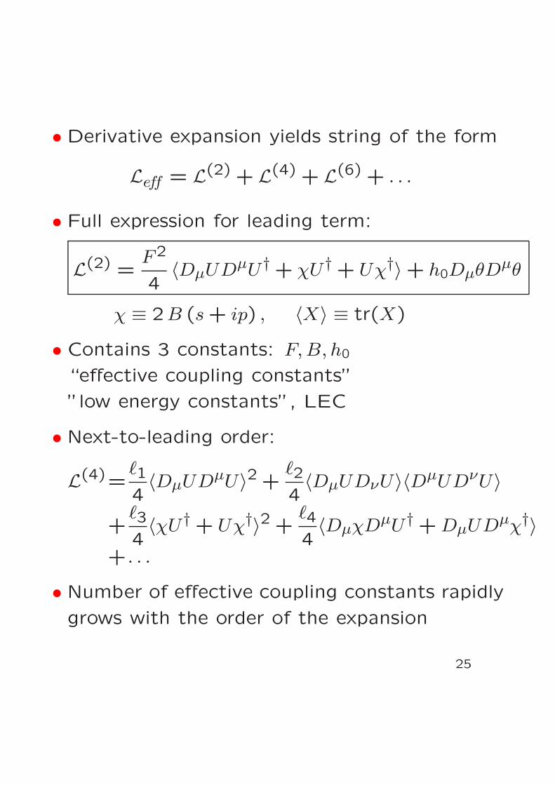
• Derivative expansion yields string of the form
Leff = L(2) + L(4) + L(6) + . . .
• Full expression for leading term:
L(2) =F2
4〈DµUDµU† + χU† + Uχ†〉 + h0DµθD
µθ
χ ≡ 2B (s+ ip) , 〈X〉 ≡ tr(X)
• Contains 3 constants: F,B, h0
“effective coupling constants”
”low energy constants”, LEC
• Next-to-leading order:
L(4)=ℓ14〈DµUDµU〉2 +
ℓ24〈DµUDνU〉〈DµUDνU〉
+ℓ34〈χU† + Uχ†〉2 +
ℓ44〈DµχDµU† +DµUD
µχ†〉+ . . .
• Number of effective coupling constants rapidly
grows with the order of the expansion
25
• Infinitely many effective coupling constants
Symmetry does not determine these
Predictivity ?
• Essential point: If Leff is known to given order
⇒ can work out low energy expansion of the
Green functions to that order (Weinberg 1979)
• NLO expressions for Fπ,Mπ involve 2 new
coupling constants: ℓ3, ℓ4.
In the ππ scattering amplitude, two further
coupling constants enter at NLO: ℓ1, ℓ2.
• Note: effective theory is a quantum field theory
Need to perform the path integral
eiSQCDv,a,s,p,θ = Neff
∫
[dπ]ei∫
dxLeff~π,v,a,s,p,θ
26
• Classical theory ⇔ tree graphs
Need to include graphs with loops
• Power counting in dimensional regularization:
Graphs with ℓ loops are suppressed by factor
p2ℓ as compared to tree graphs
⇒ Leading contributions given by tree graphs
Graphs with one loop contribute at next-to-
leading order, etc.
• The leading contribution to SQCD is given by
the sum of all tree graphs = classical action:
SQCDv, a, s, p, θ = extremumU(x)
∫
dxLeffU, v, a, s, p, θ
27
III. Illustrations
12. Some tree level calculations
A. Extracting the quark condensate from
the generating functional
• To calculate the quark condensate of the mass-
less theory, it suffices to consider the effective
action for v = a = p = θ = 0 and to take a
constant scalar external field
s =
(
mu 00 md
)
• Expansion in powers of mu and md treats
H1 =∫
d3x muuu+mddd as a perturbation
SQCD0,0,m,0,0 = S0QCD + S1
QCD + . . .
• S0QCD is independent of the quark masses
(cosmological constant)
• S1QCD is linear in the quark masses
28
• First order in mu, md ⇒ expectation value of
H1 in unperturbed ground state is relevant
S1QCD = −
∫
dx〈0|muuu+mddd |0〉
⇒ 〈0|uu |0〉 and 〈0|dd |0〉 are the coefficients of
the terms in SQCD that are linear in mu and md
B. Condensate in terms of effective theory
• Need the effective action for v = a = p = θ = 0
to first order in s
⇒ classical level of effective theory suffices.
• extremum of the classical action: U = 1
S1QCD =
∫
dxF2B(mu +md)
• comparison with
S1QCD = −
∫
dx〈0|muuu+mddd |0〉 yields
〈0|uu |0〉 = 〈0|dd |0〉 = −F2B (1)
29
C. Evaluation of Mπ at tree level
• In classical theory, the square of the mass is
the coefficient of the term in the Lagrangian
that is quadratic in the meson field:
F2
4〈χU† + Uχ†〉 =
F2B
2〈m(U† + U)〉
= F2B(mu +md)1 − ~π 2
2F2+ . . .
Hence M2π = (mu +md)B (2)
• Tree level result for Fπ:
Fπ = F (3)
• (1) + (2) + (3) ⇒ GMOR relation:
M2π =
(mu +md) |〈0|uu |0〉|F2π
30
13. Mπ beyond tree level
• The formula M2π = (mu +md)B only holds at
tree level, represents leading term in expansion
of M2π in powers of mu,md
• Disregard isospin breaking: set mu = md = m
A. Mπ to 1 loop
• Claim: at next-to-leading order, the expansion
of M2π in powers of m contains a logarithm:
M2π = M2 − 1
2
M4
(4πF)2ln
Λ 23
M2+O(M6)
M2 ≡ 2mB
• Proof: Pion mass ⇔ pole position, for instance
in the Fourier transform of 〈0|TAµa(x)Aνb(y) |0〉Suffices to work out the perturbation series for
this object to one loop of the effective theory
31
• Result (exercise # 5):
M2π = M2+
2 ℓ3M4
F2+M2
2F2
1
i∆(0,M2)+O(M6)
∆(0,M2) is the propagator at the origin
(exercise # 2):
∆(0,M2)=1
(2π)d
∫
ddp
M2 − p2 − iǫ
=i (4π)−d/2 Γ(1 − d/2)Md−2
• Contains a pole at d = 4:
Γ (1 − d/2) =2
d− 4+ . . .
• Divergent part is proportional to M2:
Md−2=M2µd−4(M/µ)d−4 = M2µd−4e(d−4) ln(M/µ)
=M2µd−41 + (d− 4) ln(M/µ) + . . .• Denote the singular factor by
λ≡ 1
2(4π)−d/2 Γ(1 − d/2)µd−4
=µd−4
16π2
1
d− 4− 1
2(ln 4π+ Γ′(1) + 1) +O(d− 4)
32
• The propagator at the origin then becomes
1
i∆(0,M2)=M2
2λ+1
16π2lnM2
µ2+O(d− 4)
• In the expression for M2π
M2π = M2+
2 ℓ3M4
F2+M2
2F2
1
i∆(0,M2)+O(M6)
the divergence can be absorbed in ℓ3:
ℓ3 = −1
2λ+ ℓ ren
3
• ℓ ren3 depends on the renormalization scale µ
ℓ ren3 =
1
64π2lnµ2
Λ23
running coupling constant
• Λ3 is the ren. group invariant scale of ℓ3
Net result for M2π
M2π = M2 − 1
2
M4
(4πF)2ln
Λ 23
M2+O(M6)
⇒M2π contains a chiral logarithm at NLO
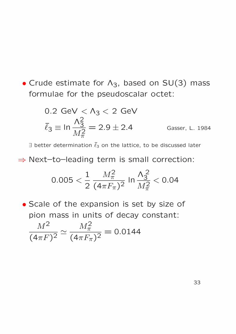
• Crude estimate for Λ3, based on SU(3) mass
formulae for the pseudoscalar octet:
0.2 GeV < Λ3 < 2 GeV
ℓ3 ≡ lnΛ2
3
M2π
= 2.9 ± 2.4 Gasser, L. 1984
∃ better determination ℓ3 on the lattice, to be discussed later
⇒ Next–to–leading term is small correction:
0.005 <1
2
M2π
(4πFπ)2ln
Λ 23
M2π< 0.04
• Scale of the expansion is set by size of
pion mass in units of decay constant:
M2
(4πF)2≃ M2
π
(4πFπ)2= 0.0144
33
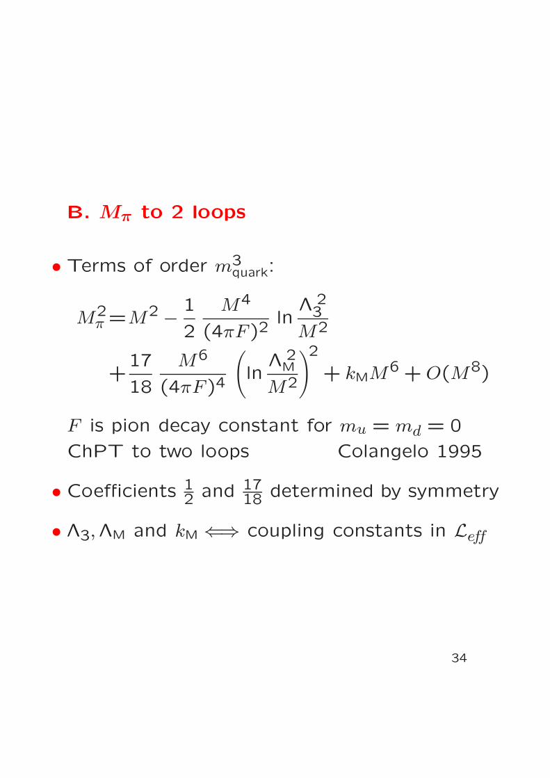
B. Mπ to 2 loops
• Terms of order m3quark:
M2π=M2 − 1
2
M4
(4πF)2ln
Λ 23
M2
+17
18
M6
(4πF)4
(
lnΛ 2
M
M2
)2
+ kMM6 +O(M8)
F is pion decay constant for mu = md = 0
ChPT to two loops Colangelo 1995
• Coefficients 12 and 17
18 determined by symmetry
• Λ3,ΛM and kM ⇐⇒ coupling constants in Leff
34
14. Fπ to one loop
• Also contains a logarithm at NLO:
Fπ=F
1− M2
16π2F2lnM2
Λ 24
+O(M4)
M2π=M2
1+M2
32π2F2lnM2
Λ 23
+O(M4)
F is pion decay constant in limit mu,md → 0
• Structure is the same, coefficients and scale of
logarithm are different
• Low energy theorem: at leading order in the
chiral expansion, the scalar radius is also de-
termined by the scale Λ4:
〈r2〉s=
6
(4πF)2
lnΛ2
4
M2− 13
12+O(M2)
Chiral symmetry relates Fπ to 〈r2〉s
What is the scalar radius ? ⇒ next section
35
15. Pion form factors
• Scalar form factor of the pion:
Fs(t) = 〈π(p′)|q q |π(p)〉 , t = (p′ − p)2
• Definition of scalar radius:
Fs(t) = Fs(0)
1 +1
6〈r2〉
st+O(t2)
• Low energy theorem:
〈r2〉s=
6
(4πF)2
lnΛ2
4
M2− 13
12+O(M2)
⇒ In massless QCD, the scalar radius diverges,because the density of the pion cloud only de-creases with a power of the distance
• Same infrared singularity also occurs in thecharge radius (e.m. current), but coefficientof the chiral logarithm is 6 times smaller:
〈r2〉s
=6
(4πF)2
lnΛ2
4
M2− 13
12+O(M2)
〈r2〉em
=1
(4πF)2
lnΛ2
6
M2− 1 +O(M2)
⇒ 〈r2〉s> 〈r2〉
emif M small enough
36
• 〈r2〉em
can be determined experimentally
〈r2〉em
= 0.439 ± 0.008 fm2
NA7 Collaboration, NP B277 (1986) 168
• Scalar form factor of the pion can be calculated
by means of dispersion theory
• Result for the slope:
〈r2〉s
= 0.61 ± 0.04 fm2
Colangelo, Gasser, L., Nucl. Phys. 2001
⇒ Corresponding value of the scale Λ4:
Λ4 = 1.26 ± 0.14GeV
37
16. Lattice results for Mπ, Fπ
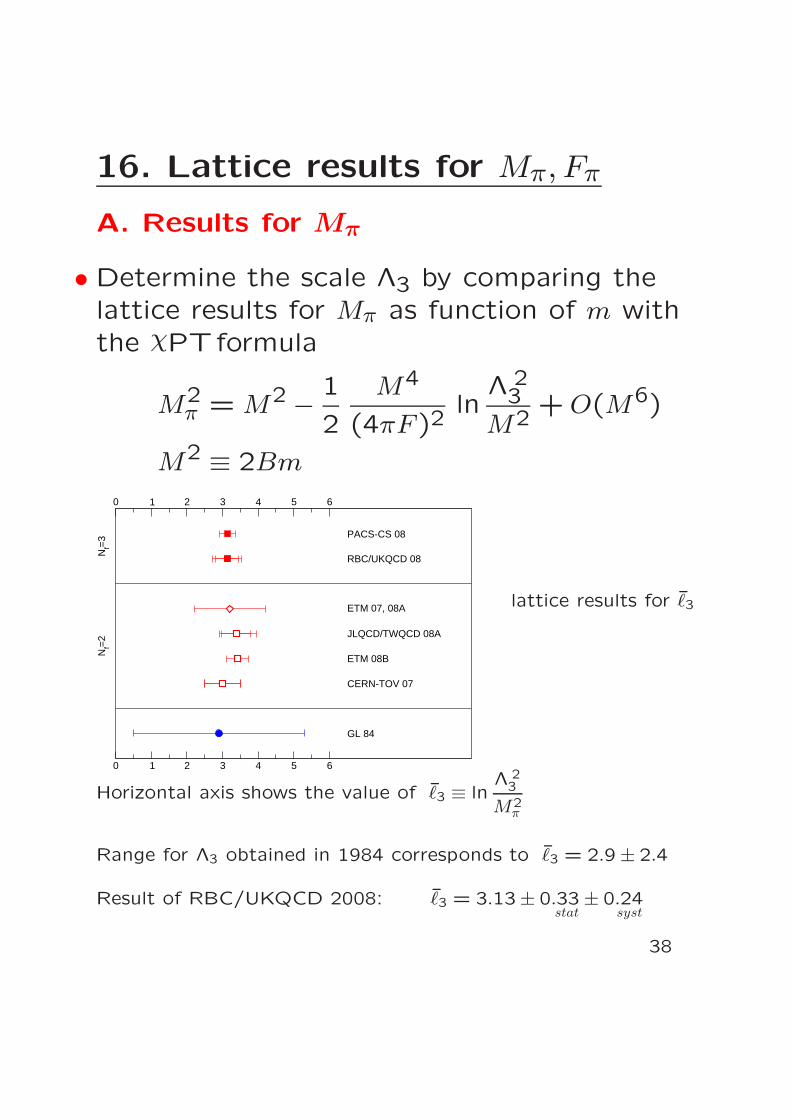
A. Results for Mπ
• Determine the scale Λ3 by comparing the
lattice results for Mπ as function of m with
the χPTformula
M2π = M2 − 1
2
M4
(4πF)2ln
Λ 23
M2+O(M6)
M2 ≡ 2Bm
0
0
1
1
2
2
3
3
4
4
5
5
6
6
CERN-TOV 07
ETM 08B
JLQCD/TWQCD 08A
ETM 07, 08A
RBC/UKQCD 08
PACS-CS 08
GL 84
Nf=
3N
f=2
lattice results for ℓ3
Horizontal axis shows the value of ℓ3 ≡ lnΛ 2
3
M2π
Range for Λ3 obtained in 1984 corresponds to ℓ3 = 2.9 ± 2.4
Result of RBC/UKQCD 2008: ℓ3 = 3.13 ± 0.33stat
± 0.24syst
38
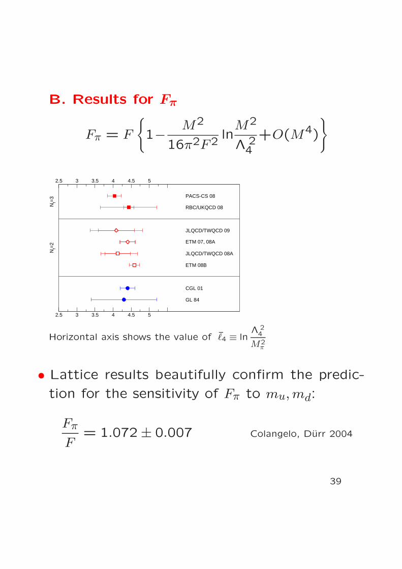
B. Results for Fπ
Fπ = F
1− M2
16π2F2lnM2
Λ 24
+O(M4)
2.5
2.5
3
3
3.5
3.5
4
4
4.5
4.5
5
5
ETM 08B
JLQCD/TWQCD 08A
ETM 07, 08A
JLQCD/TWQCD 09
RBC/UKQCD 08
PACS-CS 08
CGL 01
GL 84
Nf=
3N
f=2
Horizontal axis shows the value of ℓ4 ≡ lnΛ 2
4
M2π
• Lattice results beautifully confirm the predic-
tion for the sensitivity of Fπ to mu,md:
Fπ
F= 1.072 ± 0.007 Colangelo, Durr 2004
39
17. ππ scattering
A. Low energy scattering of pions
• Consider scattering of pions with ~p = 0
• At ~p = 0, only the S-waves survive (angular
momentum barrier). Moreover, these reduce
to the scattering lengths
• Bose statistics: S-waves cannot have I = 1,
either have I = 0 or I = 2
⇒ At ~p = 0, the ππ scattering amplitude is
characterized by two constants: a00, a20
• Chiral symmetry suppresses the interaction at
low energy: Nambu-Goldstone bosons of zero
momentum do not interact
⇒ a00, a20 disappear in the limit mu,md → 0
⇒ a00, a20 ∼M2
π measure symmetry breaking
40
B. Tree level of χPT
• Low Energy theorem Weinberg 1966:
a00=7M2
π
32πF2π
+O(M4π)
a20=− M2π
16πF2π
+O(M4π)
⇒ Chiral symmetry predicts a00, a20 in terms of Fπ
• Accuracy is limited: Low energy theorem
only specifies the first term in the expansion
in powers of the quark masses
Corrections from higher orders ?
41
C. Scattering lengths at 1 loop
• Next term in the chiral perturbation series:
a00=7M2
π
32πF2π
1 +9
2
M2π
(4πFπ)2ln
Λ20
M2π
+O(M4π)
• Coefficient of chiral logarithm unusually large
Strong, attractive final state interaction
• Scale Λ0 is determined by the coupling
constants of L(4)eff :
9
2ln
Λ20
M2π
=20
21ℓ1 +
40
21ℓ2 − 5
14ℓ3 + 2 ℓ4 +
5
2
• Information about ℓ1, . . . , ℓ4 ?
ℓ1, ℓ2 ⇐⇒ momentum dependence
of scattering amplitude
⇒ Can be determined phenomenologically
ℓ3, ℓ4 ⇐⇒ dependence of scattering
amplitude on quark masses
Have discussed their values already
42
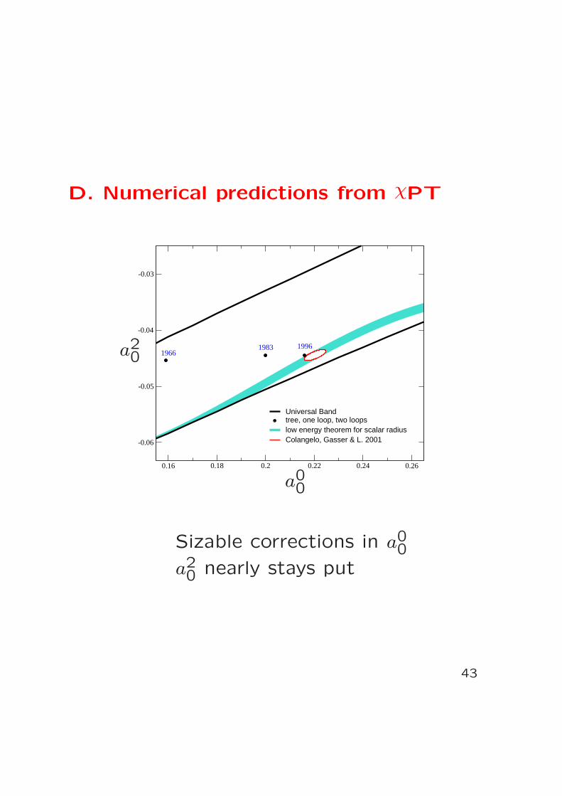
D. Numerical predictions from χPT
0.16 0.18 0.2 0.22 0.24 0.26
-0.06
-0.05
-0.04
-0.03
19661983 1996
Universal Bandtree, one loop, two loopslow energy theorem for scalar radiusColangelo, Gasser & L. 2001
a00
a20
Sizable corrections in a00a20 nearly stays put
43
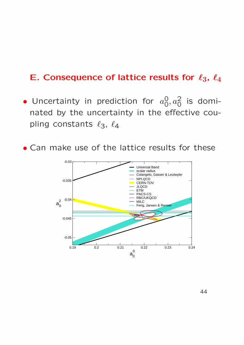
E. Consequence of lattice results for ℓ3, ℓ4
• Uncertainty in prediction for a00, a20 is domi-
nated by the uncertainty in the effective cou-
pling constants ℓ3, ℓ4
• Can make use of the lattice results for these
0.19 0.2 0.21 0.22 0.23 0.24
a00
-0.05
-0.045
-0.04
-0.035
-0.03
a20
Universal Bandscalar radiusColangelo, Gasser & LeutwylerNPLQCDCERN-TOVJLQCDETMPACS-CSRBC/UKQCDMILCFeng, Jansen & Renner
44
F. Experiments concerning a00, a2
0
• Production experiments πN → ππN ,
ψ → ππω, B → Dππ, . . .
Problem: pions are not produced in vacuo
⇒ Extraction of ππ scattering amplitude is
not simple
Accuracy rather limited
• K± → π+π−e±ν data:
CERN-Saclay, E865, NA48/2
• K± → π0π0π±, K0 → π0π0π0: cusp near
threshold, NA48/2
• π+π− atoms, DIRAC
45
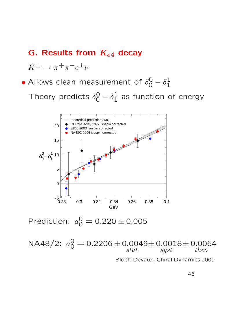
G. Results from Ke4 decay
K± → π+π−e±ν
• Allows clean measurement of δ00 − δ11
Theory predicts δ00 − δ11 as function of energy
0.28 0.3 0.32 0.34 0.36 0.38 0.4GeV
-5
0
5
10
15
20
δ00− δ1
1
theoretical prediction 2001CERN-Saclay 1977 isospin correctedE865 2003 isospin correctedNA48/2 2006 isospin corrected
Prediction: a00 = 0.220 ± 0.005
NA48/2: a00 = 0.2206± 0.0049stat
± 0.0018syst
± 0.0064theo
Bloch-Devaux, Chiral Dynamics 2009
46
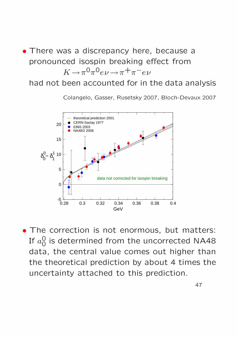
• There was a discrepancy here, because a
pronounced isospin breaking effect from
K→π0π0eν→π+π−eνhad not been accounted for in the data analysis
Colangelo, Gasser, Rusetsky 2007, Bloch-Devaux 2007
0.28 0.3 0.32 0.34 0.36 0.38 0.4GeV
-5
0
5
10
15
20
δ00− δ1
1
theoretical prediction 2001CERN-Saclay 1977E865 2003NA48/2 2006
data not corrected for isospin breaking
• The correction is not enormous, but matters:
If a00 is determined from the uncorrected NA48
data, the central value comes out higher than
the theoretical prediction by about 4 times the
uncertainty attached to this prediction.
47
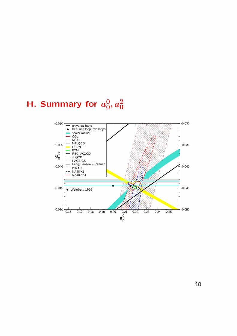
H. Summary for a00, a2
0
0.16 0.17 0.18 0.19 0.20 0.21 0.22 0.23 0.24 0.25
a00
-0.050 -0.050
-0.045 -0.045
-0.040 -0.040
-0.035 -0.035
-0.030 -0.030
a20
Weinberg 1966
universal bandtree, one loop, two loopsscalar radius CGLMILCNPLQCDCERNETMRBC/UKQCDJLQCDPACS-CSFeng, Jansen & RennerDIRACNA48 K3πNA48 Ke4
48
17. Conclusions for SU(2)×SU(2)
• Expansion in powers of mu,md yields a very
accurate low energy representation of QCD
• Lattice results confirm the GMOR relation
⇒ Mπ is dominated by the contribution from the
quark condensate
⇒ Energy gap of QCD is understood very well
• Lattice approach allows an accurate
measurement of the effective coupling constant
ℓ3 already now
• Even for ℓ4, the lattice starts becoming
competitive with dispersion theory
49
19. Expansion in powers of ms
• Theoretical reasoning
• The eightfold way is an approximate
symmetry
• The only coherent way to understand this
within QCD: ms − md, md − mu can be
treated as perturbations
• Since mu,md ≪ ms
⇒ ms can be treated as a perturbation
⇒ Expect expansion in powers of ms to work,
but convergence to be comparatively slow
• This can now also be checked on the lattice
50
• Consider the limit mu,md → 0, ms physical
• F is value of Fπ in this limit
• B is value of M2π/(mu+md) in this limit
• Σ is value of |〈0| uu |0〉| in this limit
• Exact relation: Σ = F2B
• F0, B0,Σ0: values for mu = md = ms = 0
• Paramagnetic inequalities: both F and Σ should
decrease if ms is taken smaller
F > F0 , Σ > Σ0 Jan Stern et al. 2000
• Nc → ∞: F,B,Σ become independent of ms
F/F0 → 1, B/B0 → 1, Σ/Σ0 → 1
⇒ The differences F/F0−1, B/B0−1, Σ/Σ0−1
measure the violations of the OZI rule
51
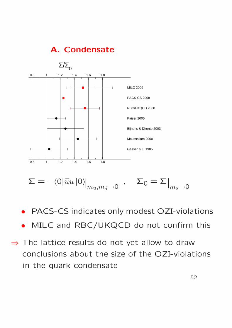
A. Condensate
0.8
0.8
1
1
1.2
1.2
1.4
1.4
1.6
1.6
1.8
1.8
RBC/UKQCD 2008
Gasser & L. 1985
Moussallam 2000
Bijnens & Dhonte 2003
Kaiser 2005
PACS-CS 2008
MILC 2009
Σ/Σ0
Σ = −〈0|uu |0〉mu,md→0
, Σ0 = Σms→0
• PACS-CS indicates only modest OZI-violations
• MILC and RBC/UKQCD do not confirm this
⇒ The lattice results do not yet allow to draw
conclusions about the size of the OZI-violations
in the quark condensate
52
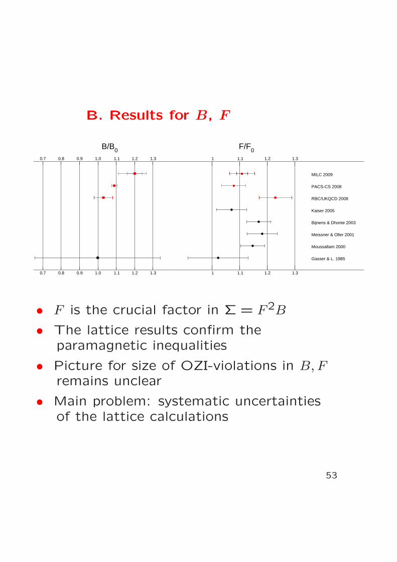
B. Results for B, F
1.0
1.0
1.1
1.1
1.2
1.2
1.3
1.3
0.9
0.9
0.8
0.8
0.7
0.7
B/B0
1
1
1.1
1.1
1.2
1.2
1.3
1.3
Gasser & L. 1985
Meissner & Oller 2001
Moussallam 2000
Bijnens & Dhonte 2003
Kaiser 2005
RBC/UKQCD 2008
PACS-CS 2008
MILC 2009
F/F0
• F is the crucial factor in Σ = F2B
• The lattice results confirm theparamagnetic inequalities
• Picture for size of OZI-violations in B,Fremains unclear
• Main problem: systematic uncertaintiesof the lattice calculations
53
• If the central value F/F0 = 1.23 of RBC/UKQCD
were confirmed within small uncertainties, we
would be faced with a qualitative puzzle:
• Fπ is the pion wave function at the origin
• FK is larger because one of the two valence
quarks is heavier → moves more slowly
→ wave function more narrow → higher at
the origin: FK/Fπ ≃ 1.19
• F/F0 = 1.23 indicates that the wave func-
tion is more sensitive to the mass of the
sea quarks than to the mass of the valence
quarks . . . very strange → most interesting
if true
• No such puzzle with the PACS-CS results
54
C. Expansion to NLO
Involves the effective coupling constants L4
and L6 of the SU(3)×SU(3) Lagrangian:
F/F0=1 +8M2
K
F20
L4 + χlog + . . .
Σ/Σ0=1 +32M2
K
F20
L6 + χlog + . . .
B/B0=1 +16M2
K
F20
(2L6 − L4) + χlog + . . .
MK is the kaon mass for mu = md = 0.
⇒ The LECS L4 and L6 measure the deviations
from the OZI-rule
55
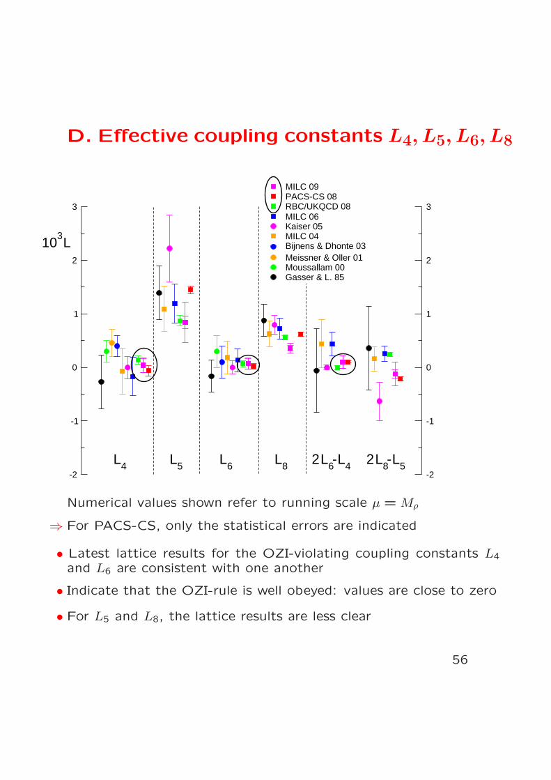
D. Effective coupling constants L4, L5, L6, L8
-2 -2
-1 -1
0 0
1 1
2 2
3 3
103L
L4 L5 L6 L8 2L6-L4 2L8-L5
MILC 09PACS-CS 08RBC/UKQCD 08MILC 06Kaiser 05MILC 04Bijnens & Dhonte 03Meissner & Oller 01Moussallam 00Gasser & L. 85
Numerical values shown refer to running scale µ = Mρ
⇒ For PACS-CS, only the statistical errors are indicated
• Latest lattice results for the OZI-violating coupling constants L4
and L6 are consistent with one another
• Indicate that the OZI-rule is well obeyed: values are close to zero
• For L5 and L8, the lattice results are less clear
56
20. Conclusions for SU(3)×SU(3)
• The crude estimates given 25 years ago for the
LECs relevant at NLO are confirmed
⇒ Expansion in powers of ms appears to work:
In all cases I know, where the calculation is un-
der control, the truncation at low order yields
a decent approximation
⇒ The picture looks coherent, also for SU(3)×SU(3)
• ms ≫ mu,md ⇒ higher orders more important
• For many observables ∃ representation to NNLO
Bijnens and collaborators
• Main problem: new LECs relevant at NNLO
∃ estimates based on resonance models
Vector meson dominance√
Scalar meson dominance ?Dependence on mu,md,ms: scalar resonances
•• Lattice results now start providing more precise
values for the LECs, but the settling of dust is
a slow process . . .
57
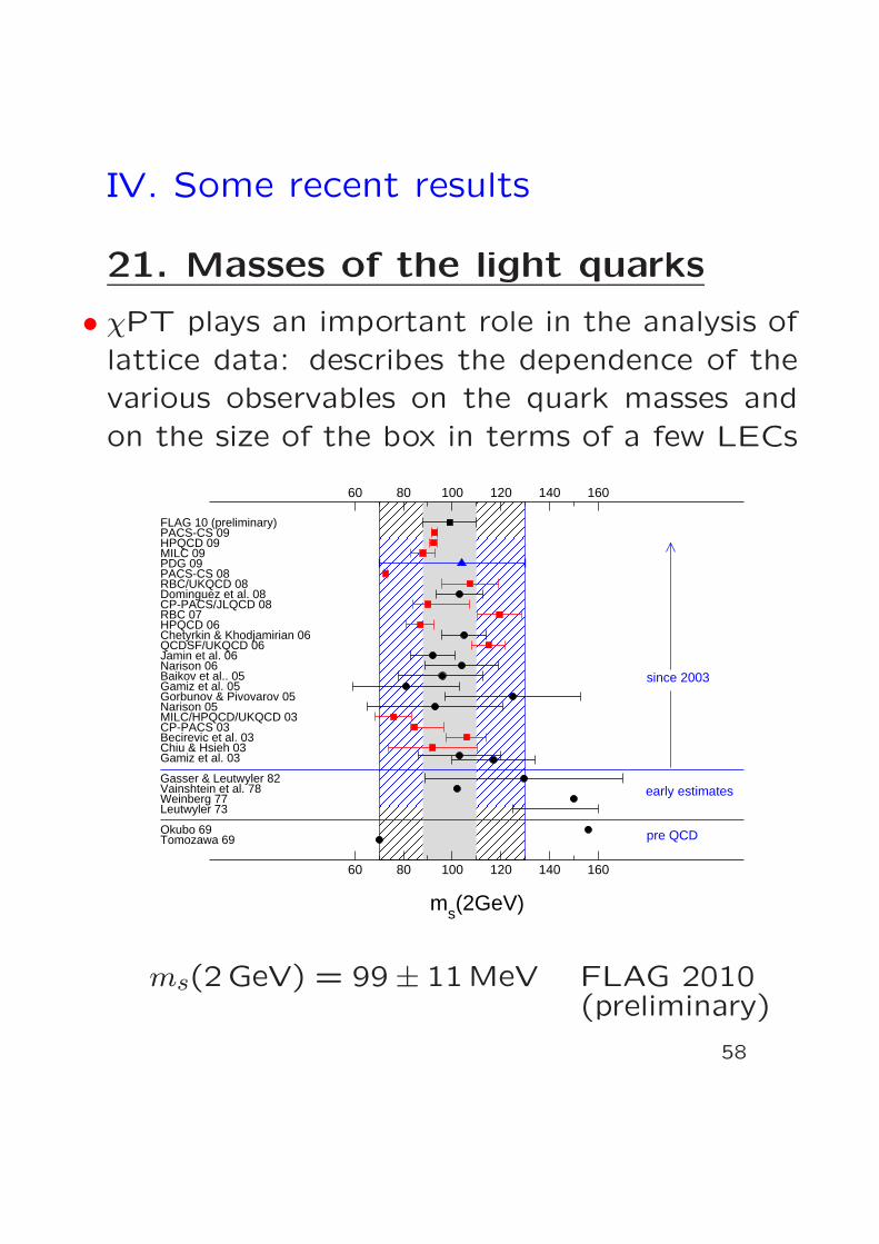
IV. Some recent results
21. Masses of the light quarks
• χPT plays an important role in the analysis of
lattice data: describes the dependence of the
various observables on the quark masses and
on the size of the box in terms of a few LECs
60
60
80
80
100
100
120
120
140
140
160
160
ms(2GeV)
Tomozawa 69Okubo 69
Gasser & Leutwyler 82
Leutwyler 73
pre QCD
early estimates
Chiu & Hsieh 03Gamiz et al. 03
Becirevic et al. 03CP-PACS 03MILC/HPQCD/UKQCD 03
Gorbunov & Pivovarov 05Narison 05
Gamiz et al. 05Baikov et al.. 05Narison 06Jamin et al. 06QCDSF/UKQCD 06Chetyrkin & Khodjamirian 06
CP-PACS/JLQCD 08RBC 07
since 2003
Weinberg 77Vainshtein et al. 78
PDG 09
RBC/UKQCD 08Dominguez et al. 08
PACS-CS 08
MILC 09
HPQCD 06
FLAG 10 (preliminary)
HPQCD 09PACS-CS 09
ms(2GeV) = 99 ± 11MeV FLAG 2010(preliminary)
58
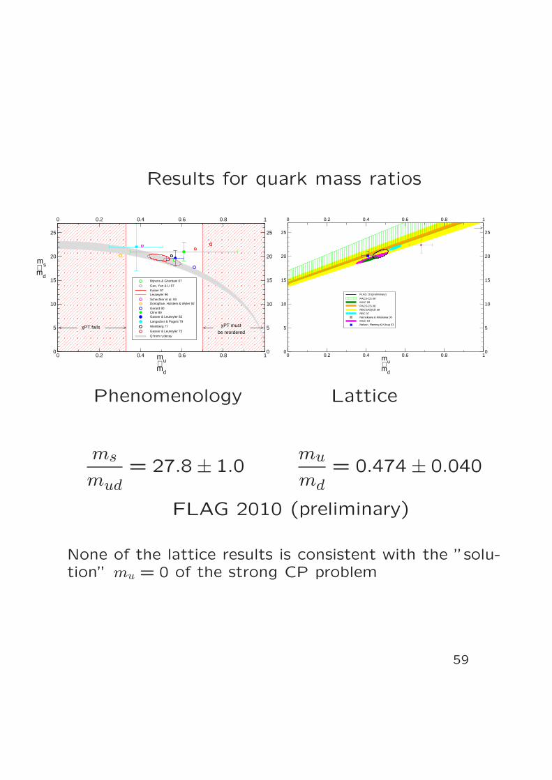
Results for quark mass ratios
0
0
0.2
0.2
0.4
0.4
0.6
0.6
0.8
0.8
1
1
mumd
0 0
5 5
10 10
15 15
20 20
25 25
msmd
χPT fails χPT must
be reordered
Bijnens & Ghorbani 07
Gao, Yan & Li 97
Kaiser 97Leutwyler 96
Schechter et al. 93Donoghue, Holstein & Wyler 92
Gerard 90Cline 89Gasser & Leutwyler 82
Langacker & Pagels 79
Weinberg 77
Gasser & Leutwyler 75
Q from η decay
0
0
0.2
0.2
0.4
0.4
0.6
0.6
0.8
0.8
1
1
mumd
0 0
5 5
10 10
15 15
20 20
25 25
FLAG 10 (preliminary)
PACS-CS 09MILC 09PACS-CS 08RBC/UKQCD 08RBC 07Namekawa & Kikukawa 06MILC 04Nelson, Fleming & Kilcup 03
Phenomenology Lattice
ms
mud= 27.8 ± 1.0
mu
md= 0.474 ± 0.040
FLAG 2010 (preliminary)
None of the lattice results is consistent with the ”solu-tion” mu = 0 of the strong CP problem
59
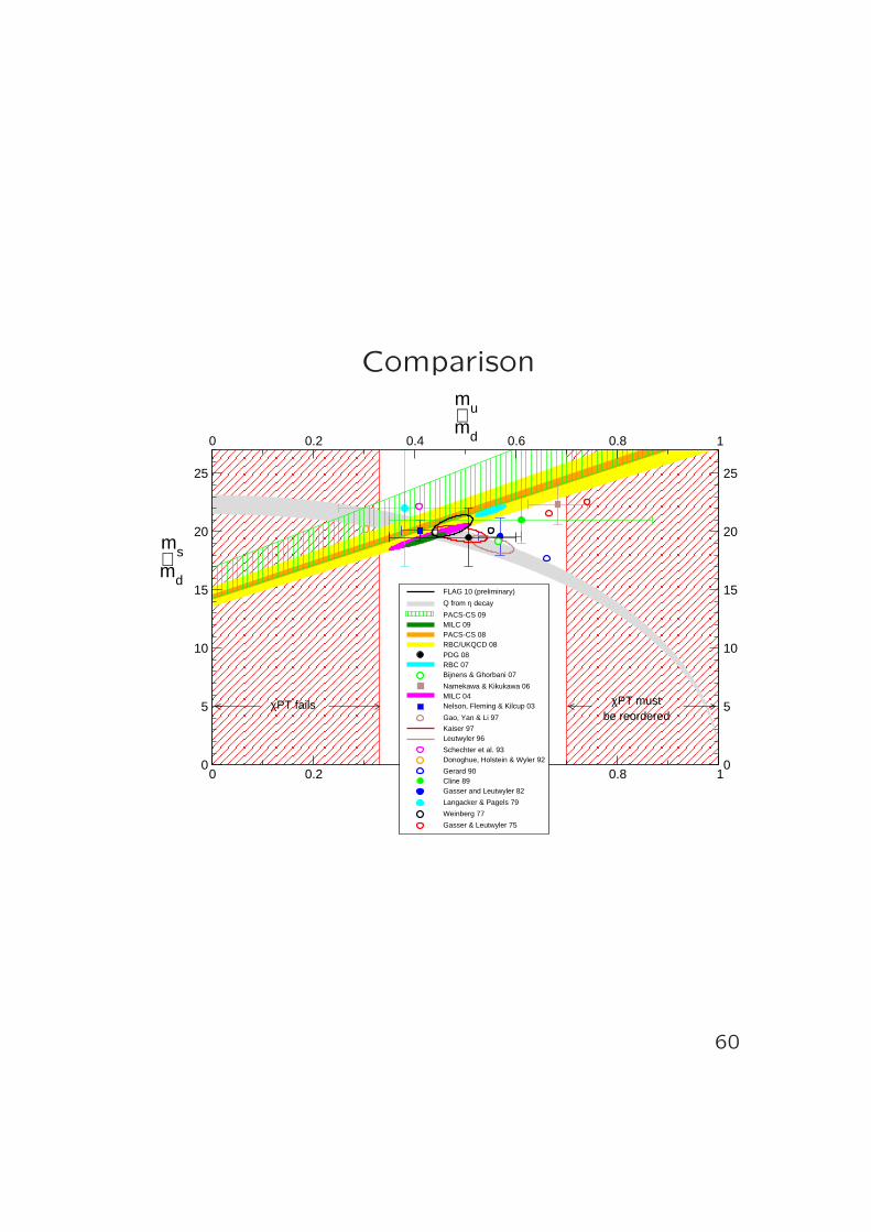
Comparison
0
0
0.2
0.2
0.4
0.4
0.6
0.6
0.8
0.8
1
1
mumd
0 0
5 5
10 10
15 15
20 20
25 25
msmd
χPT fails χPT mustbe reordered
FLAG 10 (preliminary)
Q from η decay
PACS-CS 09MILC 09PACS-CS 08RBC/UKQCD 08PDG 08RBC 07Bijnens & Ghorbani 07
Namekawa & Kikukawa 06MILC 04Nelson, Fleming & Kilcup 03
Gao, Yan & Li 97
Kaiser 97Leutwyler 96
Schechter et al. 93Donoghue, Holstein & Wyler 92
Gerard 90Cline 89Gasser and Leutwyler 82
Langacker & Pagels 79
Weinberg 77
Gasser & Leutwyler 75
60
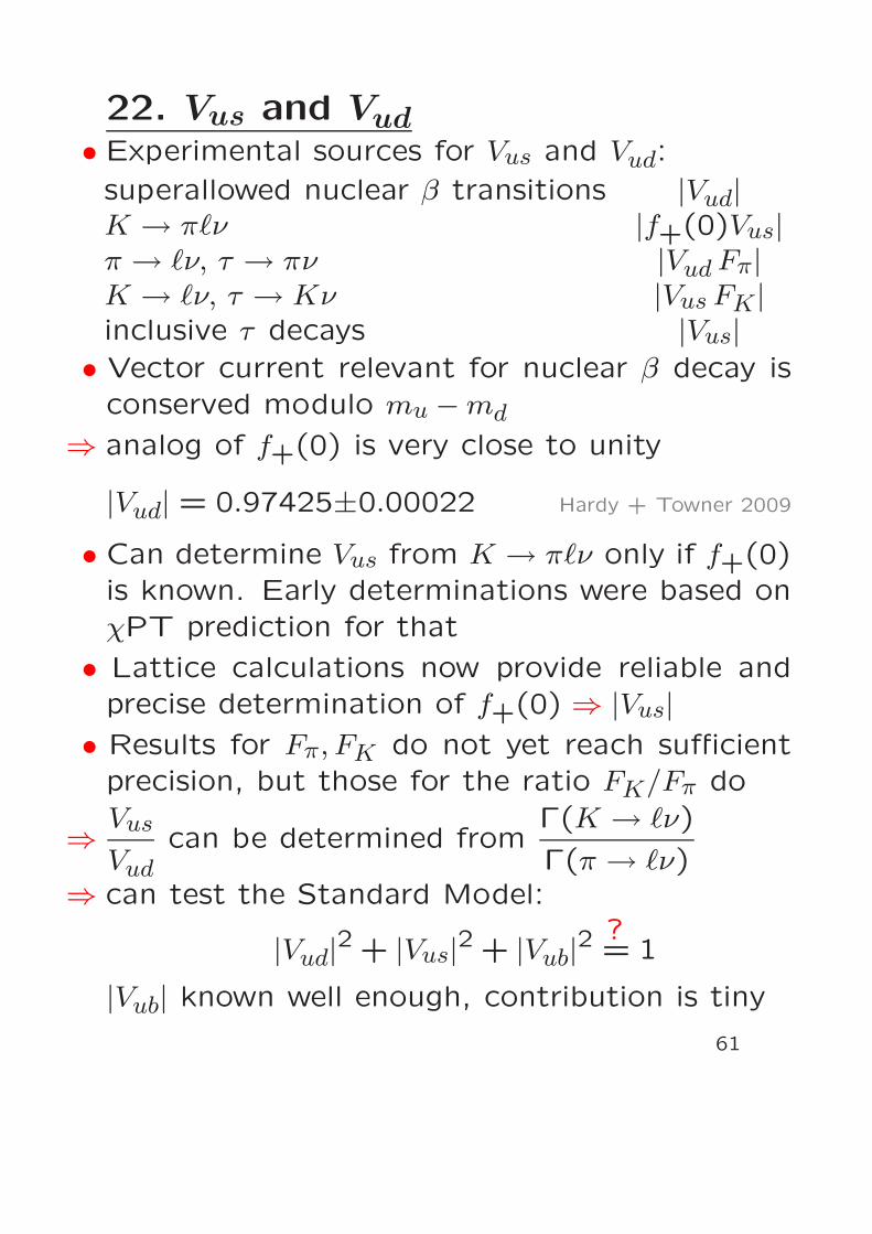
22. Vus and Vud• Experimental sources for Vus and Vud:
superallowed nuclear β transitions |Vud|K → πℓν |f+(0)Vus|π → ℓν, τ → πν |VudFπ|K → ℓν, τ → Kν |Vus FK|inclusive τ decays |Vus|
• Vector current relevant for nuclear β decay is
conserved modulo mu −md
⇒ analog of f+(0) is very close to unity
|Vud| = 0.97425±0.00022 Hardy + Towner 2009
• Can determine Vus from K → πℓν only if f+(0)
is known. Early determinations were based on
χPT prediction for that
• Lattice calculations now provide reliable and
precise determination of f+(0) ⇒ |Vus|• Results for Fπ, FK do not yet reach sufficient
precision, but those for the ratio FK/Fπ do
⇒ Vus
Vudcan be determined from
Γ(K → ℓν)
Γ(π → ℓν)⇒ can test the Standard Model:
|Vud|2 + |Vus|2 + |Vub|2 = 1?
|Vub| known well enough, contribution is tiny
61
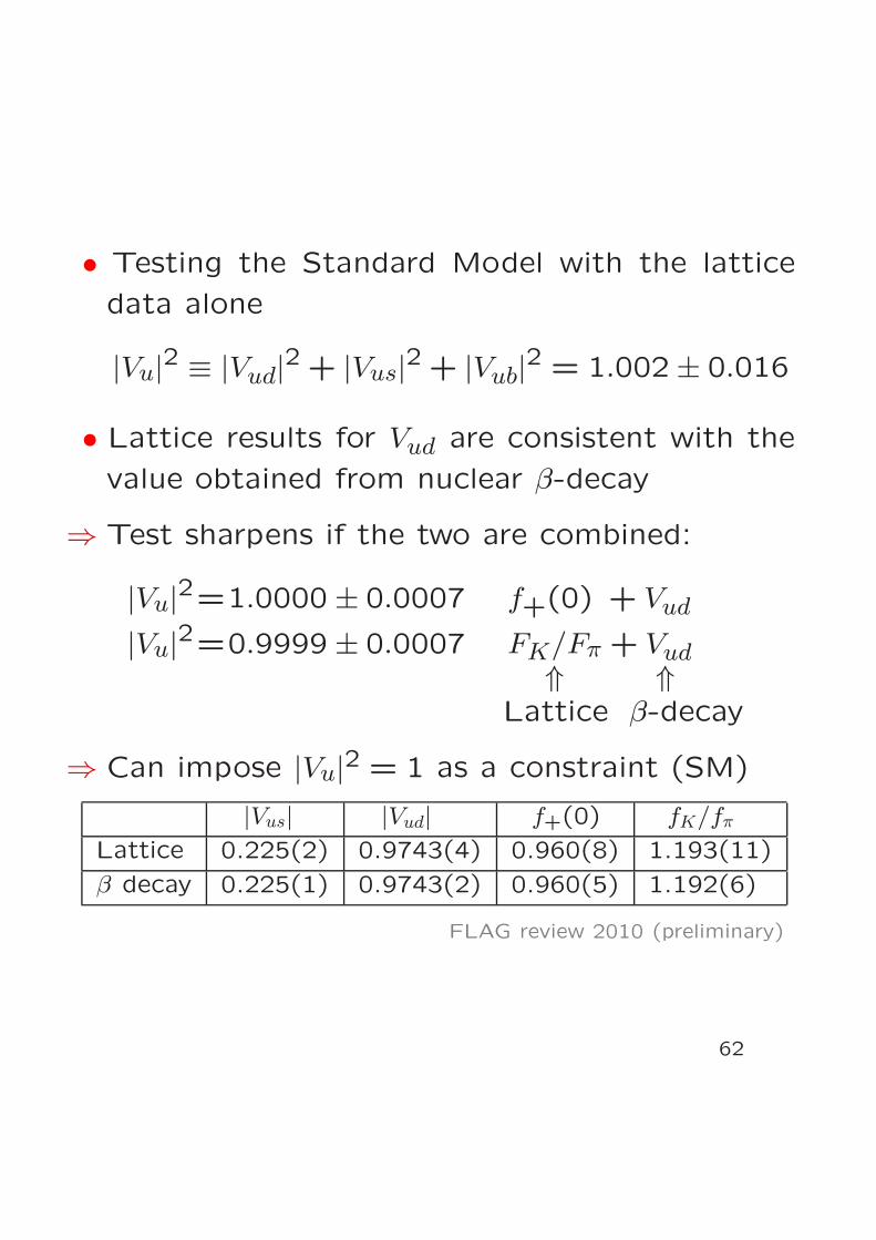
• Testing the Standard Model with the lattice
data alone
|Vu|2 ≡ |Vud|2 + |Vus|2 + |Vub|2 = 1.002 ± 0.016
• Lattice results for Vud are consistent with the
value obtained from nuclear β-decay
⇒ Test sharpens if the two are combined:
|Vu|2=1.0000 ± 0.0007 f+(0) + Vud
|Vu|2=0.9999 ± 0.0007 FK/Fπ + Vud⇑ ⇑
Lattice β-decay
⇒ Can impose |Vu|2 = 1 as a constraint (SM)
|Vus| |Vud| f+(0) fK/fπ
Lattice 0.225(2) 0.9743(4) 0.960(8) 1.193(11)
β decay 0.225(1) 0.9743(2) 0.960(5) 1.192(6)
FLAG review 2010 (preliminary)
62
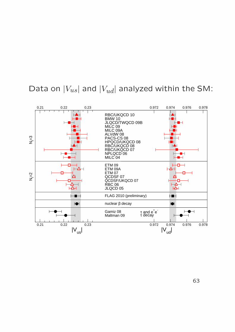
Data on |Vus| and |Vud| analyzed within the SM:
0.21
0.21
0.22
0.22
0.23
0.23
|Vus|
Nf=
3N
f=2
τ decayτ and e
+e
-
0.972
0.972
0.974
0.974
0.976
0.976
0.978
0.978
|Vud|
ETM 09
ETM 07
QCDSF/UKQCD 07
ETM 09A
QCDSF 07
RBC 06JLQCD 05
MILC 09
ALVdW 08PACS-CS 08
BMW 10
HPQCD/UKQCD 08RBC/UKQCD 08RBC/UKQCD 07NPLQCD 06MILC 04
FLAG 2010 (preliminary)
nuclear β decay
Gamiz 08Maltman 09
MILC 09A
JLQCD/TWQCD 09B
RBC/UKQCD 10
63
• Direct determination of |Vus| from τ decay:
Sort out the final states in the inclusive decay
τ → ν + hadrons:
Γ = Γ(τ → ν + strange hadrons) + rest
First term dominated by |Vus|2, rest by |Vud|2Gamiz, Jamin, Pich, Prades, SchwabMaltman, Wolfe, Banerjee, Nugent, Roney
64
23. Puzzling results on KL → πµν
• Hadronic matrix element of weak current:
〈K0|uγµs|π−〉 = (pK+pπ)µf+(t)+(pK−pπ)µf−(t)
• Scalar form factor ∼ 〈K0|∂µ(uγµs)|π−〉
f0(t) = f+(t) +t
M2K −M2
πf−(t)
• Low energy theorem Callan & Treiman 1966
f0(M2K −M2
π) =FKFπ
1 +O(mu,md)
≃ 1.19
f0(0) = f+(0) ≃ 0.96 relevant for
determination of Vus
65
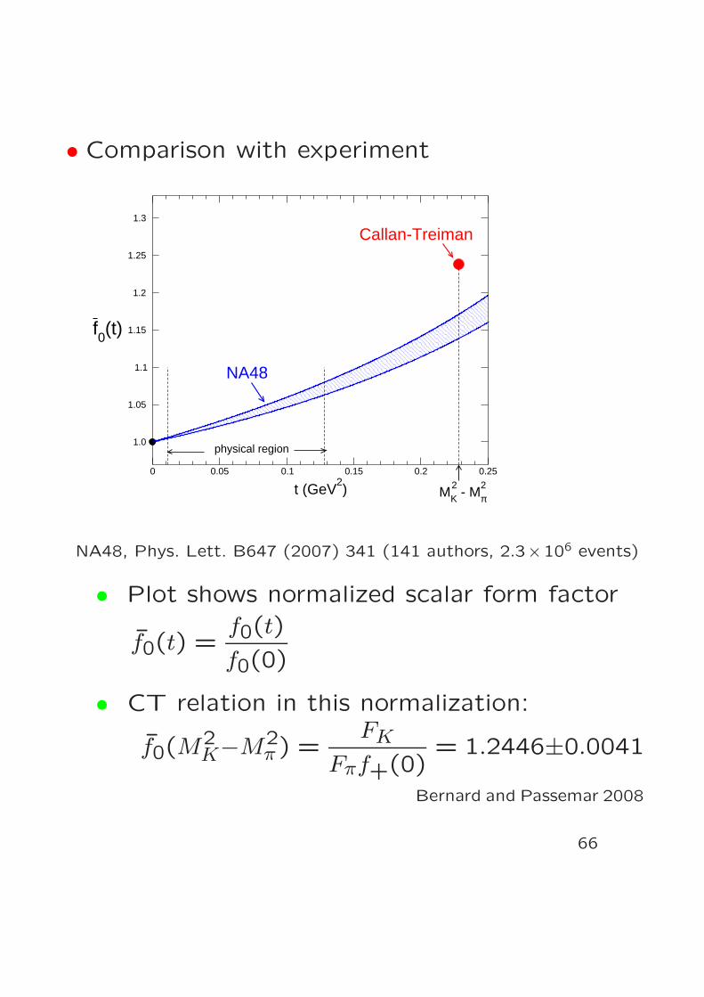
• Comparison with experiment
0 0.05 0.1 0.15 0.2 0.25
t (GeV2)
1.0
1.05
1.1
1.15
1.2
1.25
1.3
f0(t)
physical region
MK2 - M
2π
Callan-Treiman
NA48
NA48, Phys. Lett. B647 (2007) 341 (141 authors, 2.3×10⁶ events)
• Plot shows normalized scalar form factor
f0(t) =f0(t)
f0(0)
• CT relation in this normalization:
f0(M2K−M2
π) =FK
Fπf+(0)= 1.2446±0.0041
Bernard and Passemar 2008
66
• Implications
• NA48 data on KL → πµν disagree with SM
• If confirmed, the implications are dramatic:
⇒W couples also to right-handed currentsBernard, Oertel, Passemar, Stern 2006
• There are not many places where the SM
disagrees with observation, need to
investigate these carefully
• At low energies, high precision is required
67
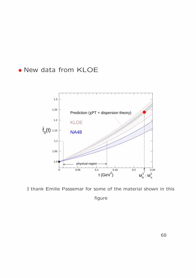
• New data from KLOE
0 0.05 0.1 0.15 0.2 0.25
t (GeV2)
1.0
1.05
1.1
1.15
1.2
1.25
1.3
f0(t)
physical region
MK2 - M
2π
NA48
KLOE
Prediction (χPT + dispersion theory)
I thank Emilie Passemar for some of the material shown in this
figure
68
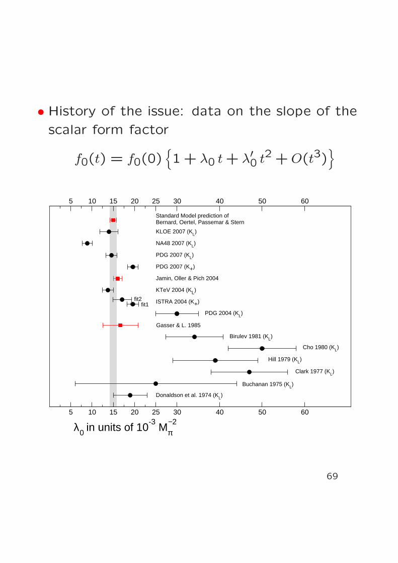
• History of the issue: data on the slope of the
scalar form factor
f0(t) = f0(0)
1 + λ0 t+ λ′0 t2 +O(t3)
10
10
15
15
20
20
30
30
40
40
50
50
60
60
5
5
25
25
λ0 in units of 10-3
Mπ−2
Gasser & L. 1985
ISTRA 2004 (K+)
KTeV 2004 (KL)
Jamin, Oller & Pich 2004
PDG 2007 (K+)
PDG 2007 (KL)
KLOE 2007 (KL)
NA48 2007 (KL)
Bernard, Oertel, Passemar & Stern
fit2fit1
PDG 2004 (KL)
Birulev 1981 (KL)
Cho 1980 (KL)
Hill 1979 (KL)
Clark 1977 (KL)
Buchanan 1975 (KL)
Donaldson et al. 1974 (KL)
Standard Model prediction of
69
24. Concluding remarks
• These lectures focused on the low energy prop-
erties of the sector with zero baryon number:
NB = 13(Nu + Nd + Ns + Nc + Nb + Nt) = 0.
Moreover, only states with Nc = Nb = Nt = 0
were discussed.
• There is considerable progress in extending
χPT to the sector with NB = 1, as well as
to nuclei, where NB = 2,3 . . .
Hint: ask Prof. Scherer for a course on these developments
• Effective theory for heavy quark bound states
• Mesons with a heavy and a light quark
• Extension from QCD to QCD + QED
70
• Combine χPT with dispersion theory
Example: form factors relevant for K → πℓν
f0(t) = f0(0)
1 + λ0 t+ λ′0 t2 + . . .
χPT: λ0 ↔ NLO, λ′0 ↔ NNLO
Dispersion theory implies very strong
correlation between λ0 and λ′0Abbas, Ananthanarayan, Caprini, Imsong 2010
• Dispersive analysis of ππ and πK scattering,
η → 3π, . . .
If time permits, I can explain how dispersion theory can be used to
extend the χPT result for the ππ scattering lengths to a
model-independent prediction for mass and width of the σ meson
71
Exercises
1. Evaluate the positive frequency part of the massless propagator
∆+(z,0) =i
(2π)3
∫
d3k
2k0e−ikz , k0 = |~k|
for Imz0 < 0. Show that the result can be represented as
∆+(z,0) =1
4πiz2
2. Evaluate the d-dimensional propagator
∆(z,M) =
∫
ddk
(2π)de−ikz
M2 − k2 − iǫ
at the origin and verify the representation
∆(0,M) =i
4πΓ
(
1 − d
2
)
(
M2
4π
)d2−1
How does this expression behave when d→ 4 ?
72
3. Leading order effective Lagrangian:
L(2) =F 2
4〈DµUD
µU† + χU† + Uχ†〉 + h0DµθDµθ
DµU = ∂µU − i(vµ + aµ)U + i U(vµ − aµ)
χ = 2B (s+ ip)
Dµθ = ∂µθ+ 2〈aµ〉〈X〉 = trX
• Take the space-time independent part of the external fields(x) to be isospin symmetric (i. e. set mu = md = m):
s(x) = m1 + s(x)
• Expand U = exp i φ/F in powers of φ = ~φ · ~τ and check that,in this normalization of the field φ, the kinetic part takes thestandard form
L(2) = 12∂µ~φ · ∂µ~φ− 1
2M2~φ2 + . . .
with M2 = 2mB.
• Draw the graphs for all of the interaction vertices containingup to four of the fields φ, vµ, aµ, s, p, θ.
73
4. Show that the classical field theory belonging to the QCD La-grangian in the presence of external fields is invariant under
v′µ + a′µ = VR(vµ + aµ)V†R
− i∂µVRV†R
v′µ − a′µ = VL(vµ − aµ)V†L− i∂µVLV
†L
s′ + i p′ = VR(s+ i p)V †L
q′R = VR qR(x)
q′L = VL qL
where VR, VL are space-time dependent elements of U(3).
5. Evaluate the pion mass to NLO of χPT . Draw the relevantgraphs and verify the representation
M2π = M2 +
2 ℓ3M4
F 2+
M2
2F 2
1
i∆(0,M2) +O(M6)
6. Start from the symmetry property of the effective action,
SQCDv′, a′, s′, p′, θ′ = SQCDv, a, s, p, θ −∫
dx〈βΩ〉,
and show that this relation in particular implies the Ward identity
∂xµ〈0|TAµa(x)Pb(y) |0〉 = −14i δ(x− y)〈0|qλa, λbq |0〉
+ 〈0|Tq(x) iγ5m, 12λaq(x)Pb(y) |0〉
a = 1, . . . ,8, b = 0, . . . ,8
7. What is the Ward identity obeyed by the singlet axial current,
∂xµ〈0|TAµ0(x)Pb(y) |0〉 = ?
74