7- 1

© ADMN 3116, Anton Miglo

ADMN 3116: Financial Management 1

Lecture 7: Portfolio selection

Anton Miglo

Fall 2014

7- 2

© ADMN 3116, Anton Miglo

Topics Covered

Efficient Set of Portfolios Sharpe ratio and optimal portfolio Optimal portfolio with risk-free asset available Excel: Solver Additional readings: ch. 10-11 B

7- 3

© ADMN 3116, Anton Miglo

Diversification

7- 4

© ADMN 3116, Anton Miglo

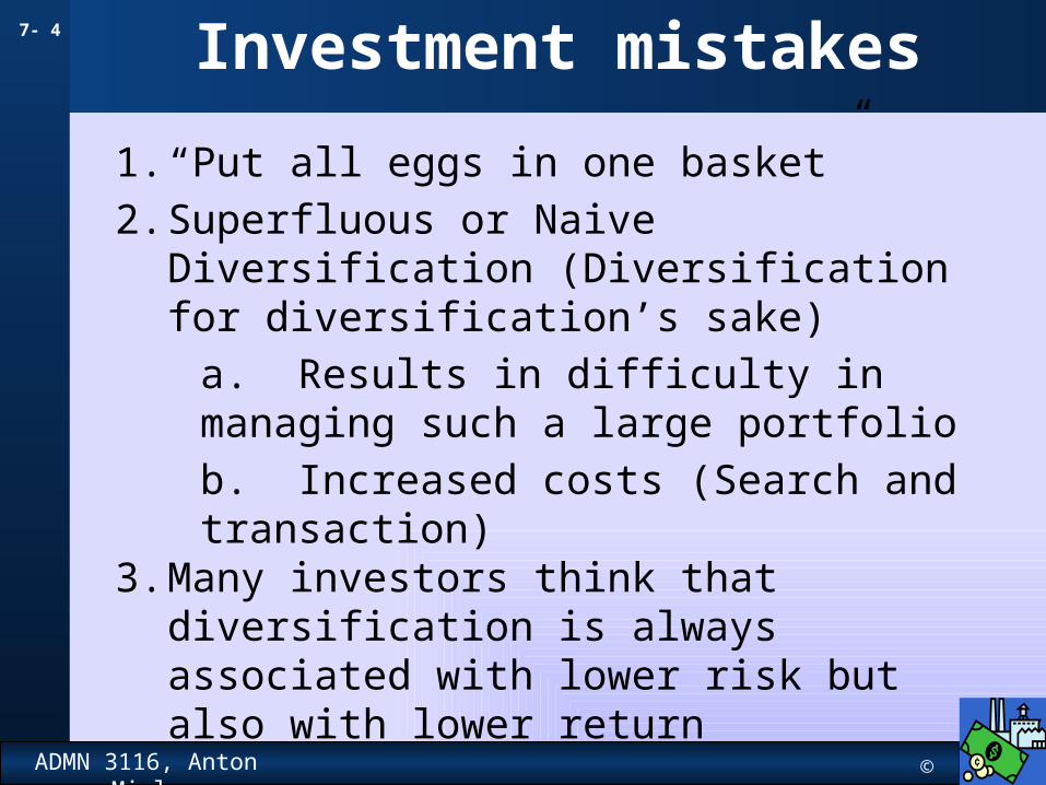
Investment mistakes

1. “Put all eggs in one basket”

2. Superfluous or Naive Diversification (Diversification for diversification’s sake)

a. Results in difficulty in managing such a large portfolio

b. Increased costs (Search and transaction)3. Many investors think that diversification is

always associated with lower risk but also with lower return

7- 5

© ADMN 3116, Anton Miglo

Correlation

OntarioQuebec

7- 6

© ADMN 3116, Anton Miglo

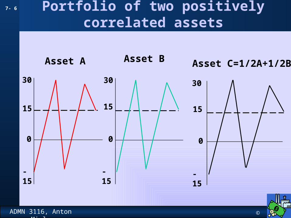
Portfolio of two positively correlated assets

Asset A

0

15

30

-15

Asset B

0

15

30

-15

Asset C=1/2A+1/2B

0

15

30

-15

7- 7

© ADMN 3116, Anton Miglo

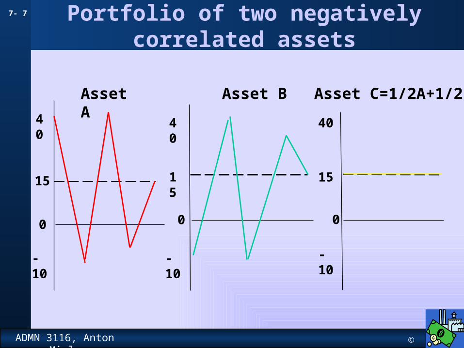
Portfolio of two negatively correlated assets

-10

15

15

40

4040

15

0

-10

Asset A

0

Asset B

-10

0

Asset C=1/2A+1/2B

7- 8

© ADMN 3116, Anton Miglo

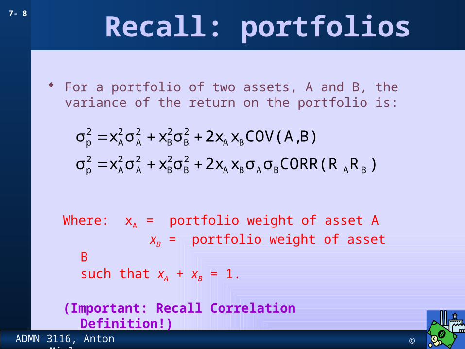
Recall: portfolios

For a portfolio of two assets, A and B, the variance of the return on the portfolio is:

Where: xA = portfolio weight of asset A

xB = portfolio weight of asset B

such that xA + xB = 1.

(Important: Recall Correlation Definition!)

)RCORR(Rσσx2xσxσxσ

B)COV(A,x2xσxσxσ

BABABA2B

2B

2A

2A

2p

BA2B

2B

2A

2A

2p

7- 9

© ADMN 3116, Anton Miglo

The Markowitz Efficient Frontier

The Markowitz Efficient frontier is the set of portfolios with the maximum return for a given risk AND the minimum risk given a return.

For the plot, the upper left-hand boundary is the Markowitz efficient frontier.

All the other possible combinations are inefficient. That is, investors would not hold these portfolios because they could get either more return for a given level of risk or less risk for a given level of return.

7- 10

© ADMN 3116, Anton Miglo

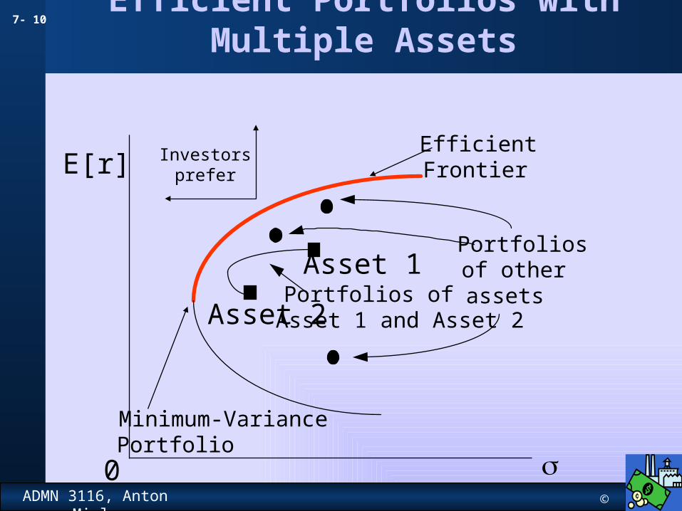
Efficient Portfolios with Multiple Assets

E[r]

s0

Asset 1

Asset 2Portfolios ofAsset 1 and Asset 2

Portfoliosof otherassets

EfficientFrontier

Minimum-VariancePortfolio

Investorsprefer

7- 11

© ADMN 3116, Anton Miglo

Excel

Solver

11

7- 12

© ADMN 3116, Anton Miglo

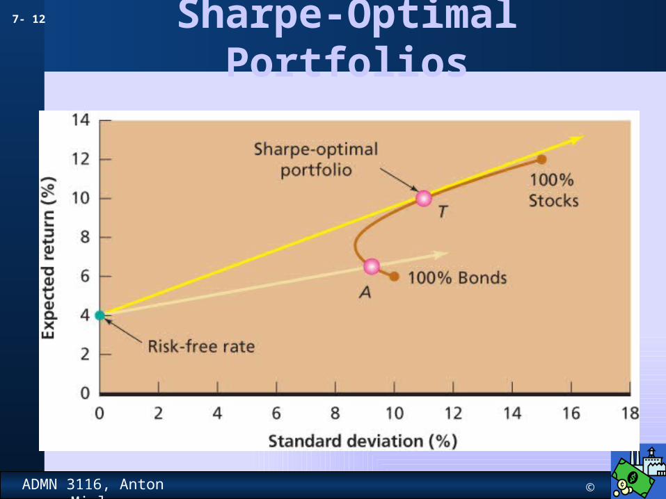
Sharpe-Optimal Portfolios

7- 13

© ADMN 3116, Anton Miglo

Example: Solving for a Sharpe-Optimal Portfolio

From a previous chapter, we know that for a 2-asset portfolio:

)R,CORR(Rσσx2xσxσx

r -)E(Rx)E(Rx

σ

r-)E(RRatio Sharpe

)R,CORR(Rσσx2xσxσxσ : VariancePortfolio

)E(Rx)E(Rx)E(R :Return Portfolio

BSBSBS2B

2B

2S

2S

fBBSS

P

fp

BSBSBS2B

2B

2S

2S

2P

BBssp

So, now our job is to choose the weight in asset S that maximizes the Sharpe Ratio.

We could use calculus to do this, or we could use Excel.

7- 14

© ADMN 3116, Anton Miglo

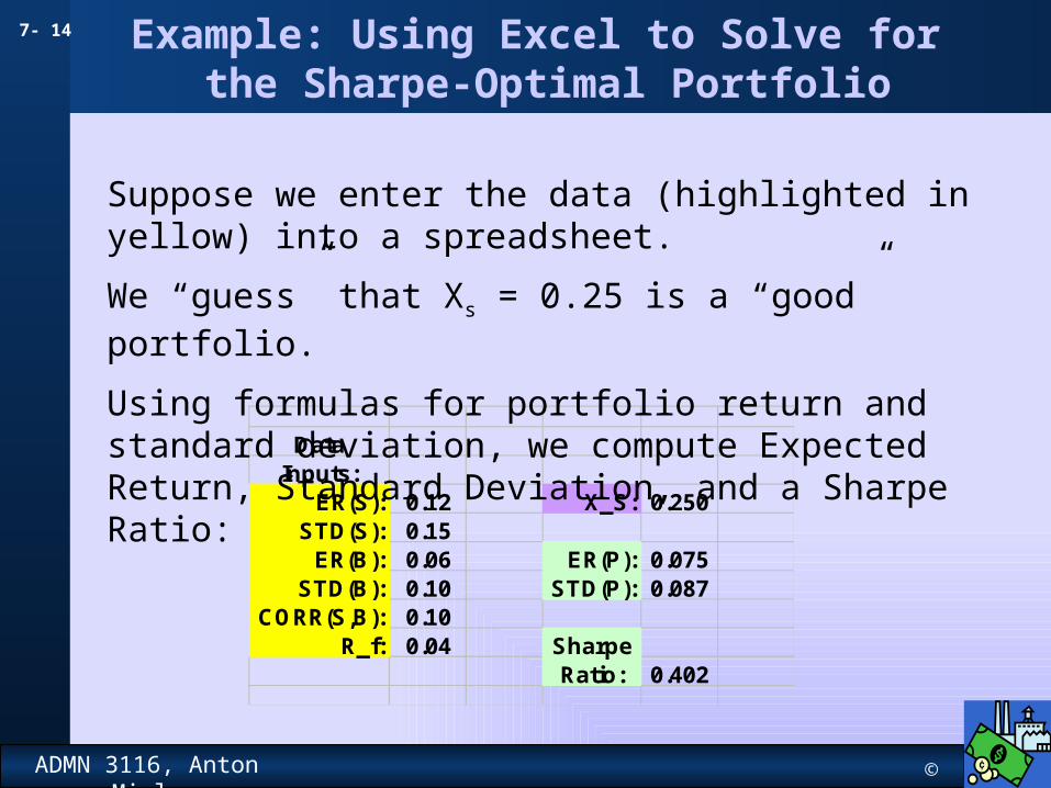
Example: Using Excel to Solve for the Sharpe-Optimal Portfolio

DataInputs:

ER(S): 0.12 X_S: 0.250STD(S): 0.15

ER(B): 0.06 ER(P): 0.075STD(B): 0.10 STD(P): 0.087

CORR(S,B): 0.10R_f: 0.04 Sharpe

Ratio: 0.402

Suppose we enter the data (highlighted in yellow) into a spreadsheet.

We “guess” that Xs = 0.25 is a “good” portfolio.

Using formulas for portfolio return and standard deviation, we compute Expected Return, Standard Deviation, and a Sharpe Ratio:

7- 15

© ADMN 3116, Anton Miglo

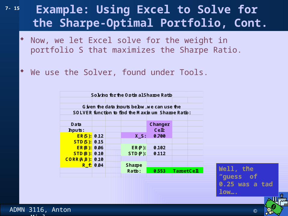
Example: Using Excel to Solve for the Sharpe-Optimal Portfolio, Cont.

Now, we let Excel solve for the weight in portfolio S that maximizes the Sharpe Ratio.

We use the Solver, found under Tools.

Data ChangerInputs: Cell:

ER(S): 0.12 X_S: 0.700STD(S): 0.15

ER(B): 0.06 ER(P): 0.102STD(B): 0.10 STD(P): 0.112

CORR(A,B): 0.10R_f: 0.04 Sharpe

Ratio: 0.553

Solving for the Optimal Sharpe Ratio

Given the data inputs below, we can use theSOLVER function to find the Maximum Sharpe Ratio:

Target Cell Well, the “guess” of 0.25 was a tad low….