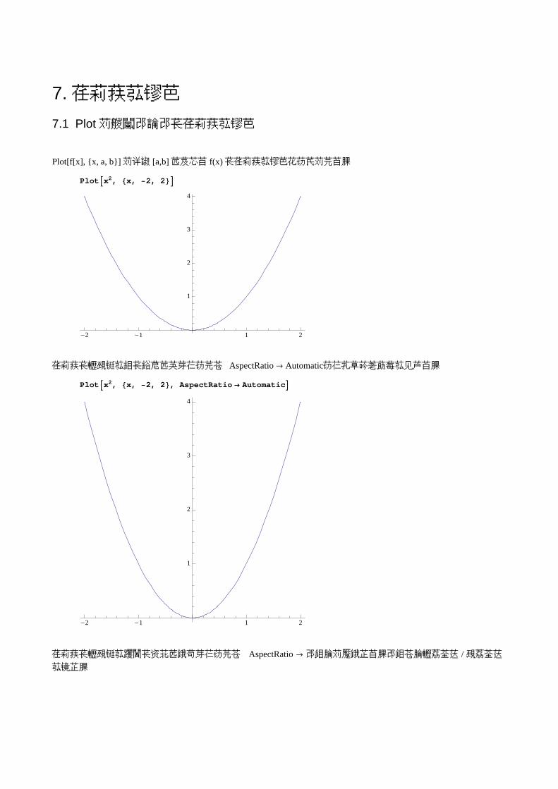
7. グラフを描く

7.1 Plot で１変数関数のグラフを描く

Plot[f[x], {x, a, b}] で区間 [a,b] における f(x) のグラフを描くことができる。

PlotAx2, 8x, -2, 2<E

-2 -1 1 2

1

2

3

4

グラフの縦横比を値の通りにしたいときは AspectRatio ® Automaticというオプションを加える。

PlotAx2, 8x, -2, 2<, AspectRatio ® AutomaticE

-2 -1 1 2

1

2

3

4

グラフの縦横比を自分の好みに定めたいときは AspectRatio ® 数値　で指定する。数値は　縦サイズ / 横サイズ

を表す。

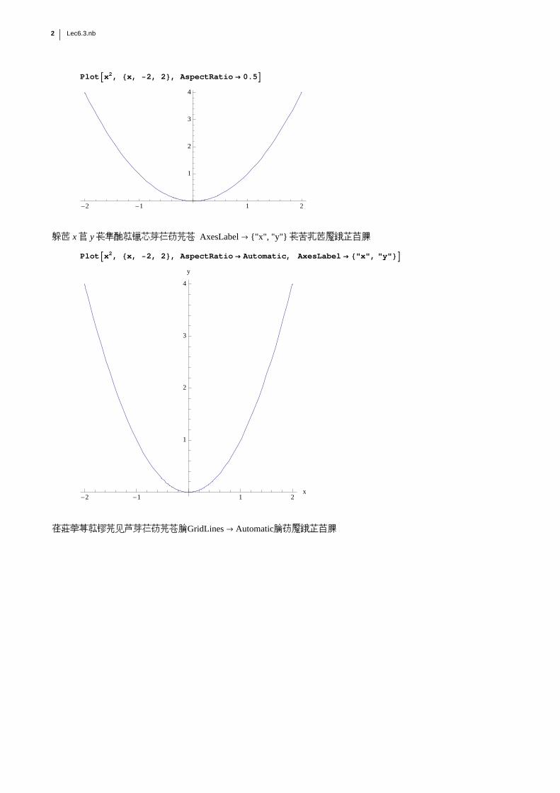
PlotAx2, 8x, -2, 2<, AspectRatio ® 0.5E

-2 -1 1 2

1

2

3

4

軸に x や y の名前を付けたいときは AxesLabel ® {"x", "y"} のように指定する。

PlotAx2, 8x, -2, 2<, AspectRatio ® Automatic, AxesLabel ® 8"x", "y"<E

-2 -1 1 2x

1

2

3

4

y

グリッドを描き加えたいときは　GridLines ® Automatic　と指定する。

2 Lec6.3.nb

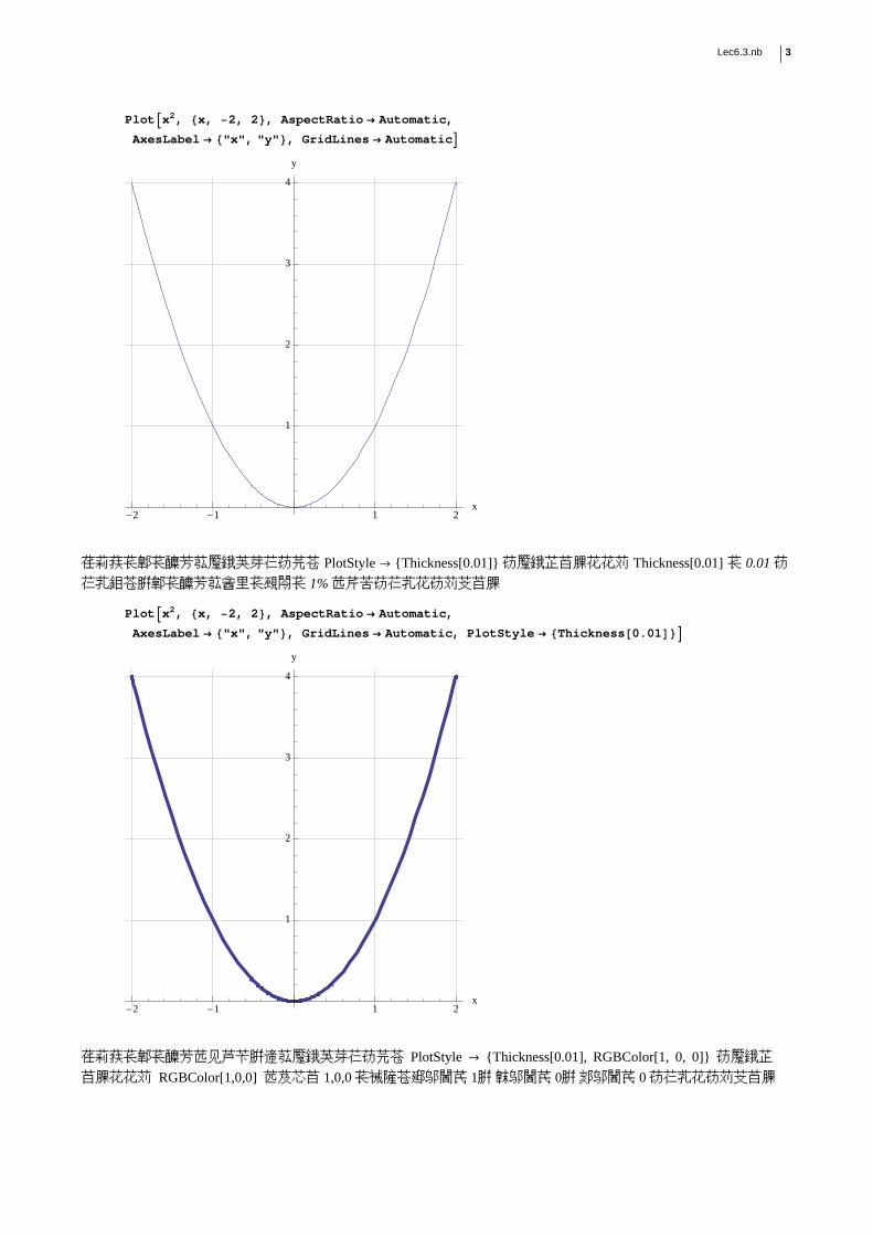
PlotAx2, 8x, -2, 2<, AspectRatio ® Automatic,

AxesLabel ® 8"x", "y"<, GridLines ® AutomaticE

-2 -1 1 2x

1

2

3

4

y

グラフの線の太さを指定したいときは PlotStyle ® {Thickness[0.01]} と指定する。ここで Thickness[0.01] の 0.01 と

いう値は、線の太さを全体の横幅の 1% にせよということである。

PlotAx2, 8x, -2, 2<, AspectRatio ® Automatic,

AxesLabel ® 8"x", "y"<, GridLines ® Automatic, PlotStyle ® 8Thickness@0.01D<E

-2 -1 1 2x

1

2

3

4

y

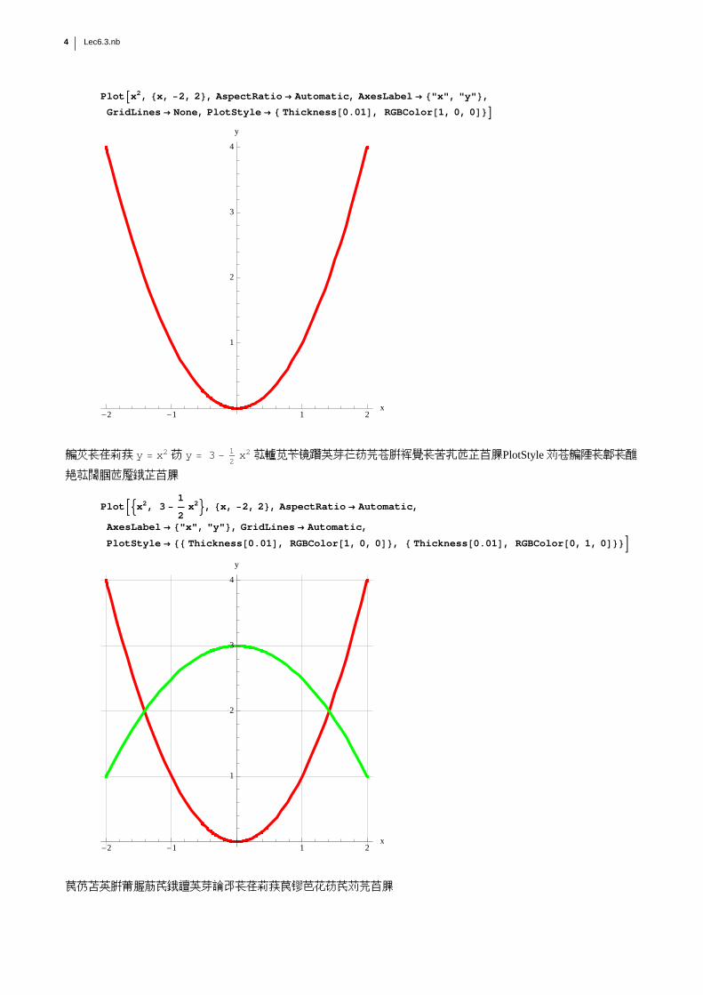
グラフの線の太さに加えて、色を指定したいときは PlotStyle ® {Thickness[0.01], RGBColor[1, 0, 0]} と指定す

る。ここで RGBColor[1,0,0] における 1,0,0 の意味は赤成分が 1、 緑成分が 0、 青成分が 0 ということである。

Lec6.3.nb 3

PlotAx2, 8x, -2, 2<, AspectRatio ® Automatic, AxesLabel ® 8"x", "y"<,GridLines ® None, PlotStyle ® 8 Thickness@0.01D, RGBColor@1, 0, 0D<E

-2 -1 1 2x

1

2

3

4

y

２つのグラフ y = x2と y = 3 -12

x2を重ねて表示したいときは、以下のようにする。PlotStyle では２本の線の属

性を別々に指定する。

PlotB:x2, 3 -1

2 x2>, 8x, -2, 2<, AspectRatio ® Automatic,

AxesLabel ® 8"x", "y"<, GridLines ® Automatic,

PlotStyle ® 88 Thickness@0.01D, RGBColor@1, 0, 0D<, 8 Thickness@0.01D, RGBColor@0, 1, 0D<<F

-2 -1 1 2x

1

2

3

4

y

もちろん、ユーザが定義した関数のグラフも描くことができる。

4 Lec6.3.nb

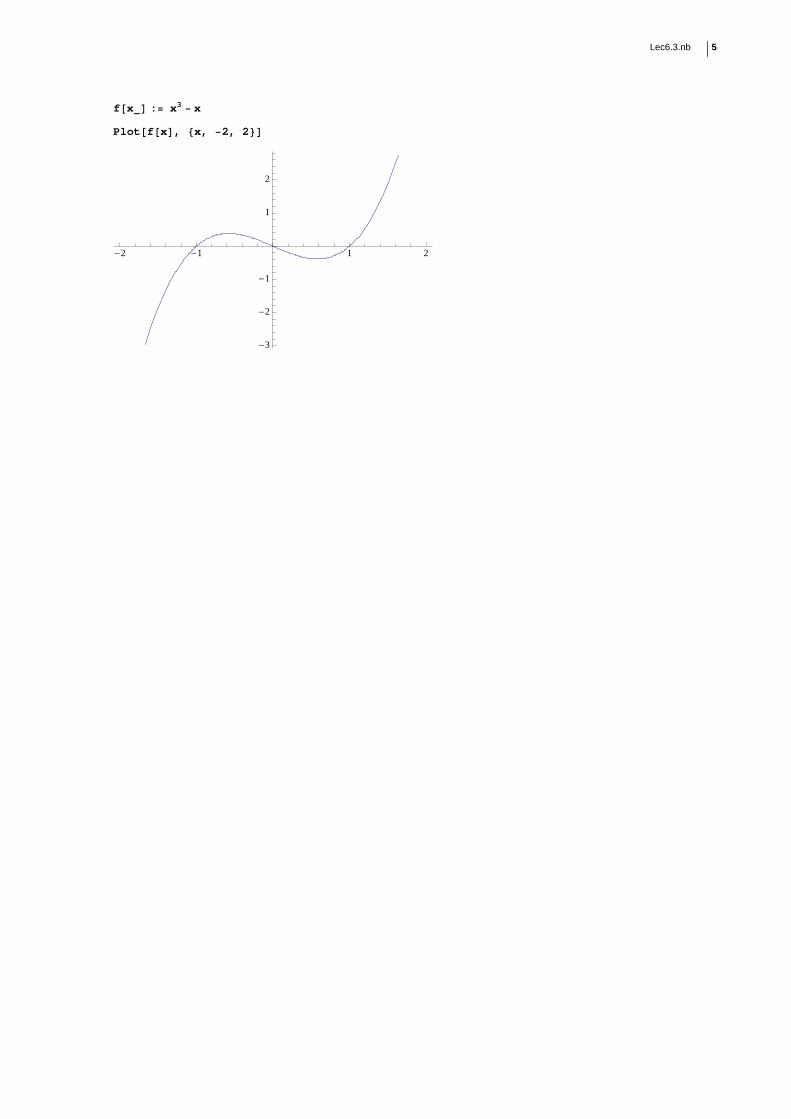
f@x_D := x3 - x

Plot@f@xD, 8x, -2, 2<D

-2 -1 1 2

-3

-2

-1

1

2

Lec6.3.nb 5

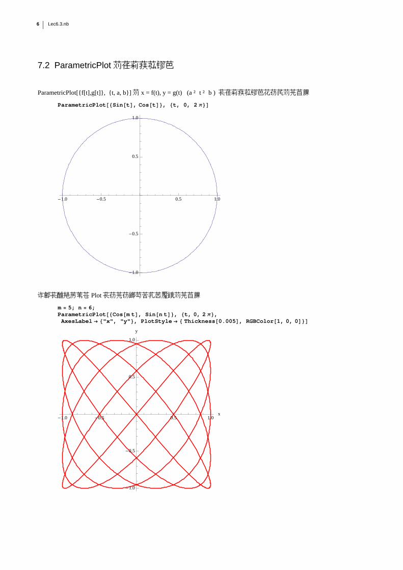
7.2 ParametricPlot でグラフを描く

ParametricPlot[{f[t],g[t]}, {t, a, b}] で x = f(t), y = g(t) (a ² t ² b ) のグラフを描くことができる。

ParametricPlot@8Sin@tD, Cos@tD<, 8t, 0, 2 Π<D

-1.0 -0.5 0.5 1.0

-1.0

-0.5

0.5

1.0

曲線の属性などは Plot のときと同じように指定できる。

m = 5; n = 6;ParametricPlot@8Cos@m tD, Sin@n tD<, 8t, 0, 2 Π<,AxesLabel ® 8"x", "y"<, PlotStyle ® 8 Thickness@0.005D, RGBColor@1, 0, 0D<D

-1.0 -0.5 0.5 1.0x

-1.0

-0.5

0.5

1.0

y

6 Lec6.3.nb

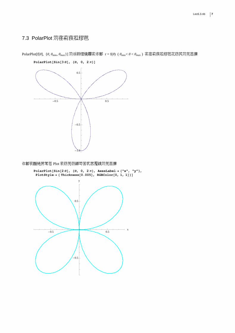
7.3 PolarPlot でグラフを描く

PolarPlot[f[Θ], {Θ, Θmin, Θmax}] で極座標表示の曲線 r = f(Θ) ( Θmin< Θ < Θmax ) のグラフを描くことができる。

PolarPlot@Sin@3 ΘD, 8Θ, 0, 2 Π<D

-0.5 0.5

-1.0

-0.5

0.5

曲線の属性などは Plot のときと同じように指定できる。

PolarPlot@Sin@2 ΘD, 8Θ, 0, 2 Π<, AxesLabel ® 8"x", "y"<,PlotStyle ® 8 Thickness@0.005D, RGBColor@0, 1, 1D<D

-0.5 0.5x

-0.5

0.5

y

Lec6.3.nb 7

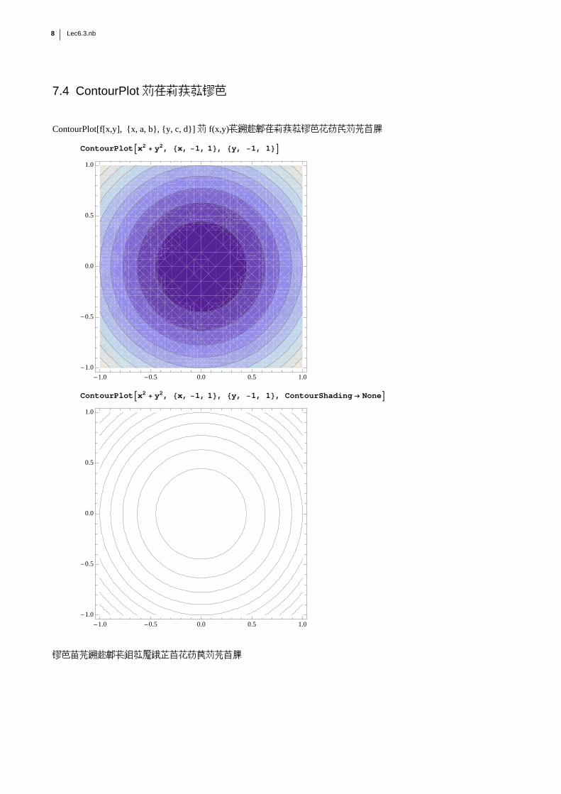
7.4 ContourPlot でグラフを描く

ContourPlot[f[x,y], {x, a, b}, {y, c, d}] で f(x,y)の等高線グラフを描くことができる。

ContourPlotAx2 + y2, 8x, -1, 1<, 8y, -1, 1<E

-1.0 -0.5 0.0 0.5 1.0

-1.0

-0.5

0.0

0.5

1.0

ContourPlotAx2 + y2, 8x, -1, 1<, 8y, -1, 1<, ContourShading ® NoneE

-1.0 -0.5 0.0 0.5 1.0

-1.0

-0.5

0.0

0.5

1.0

描くべき等高線の値を指定することもできる。

8 Lec6.3.nb

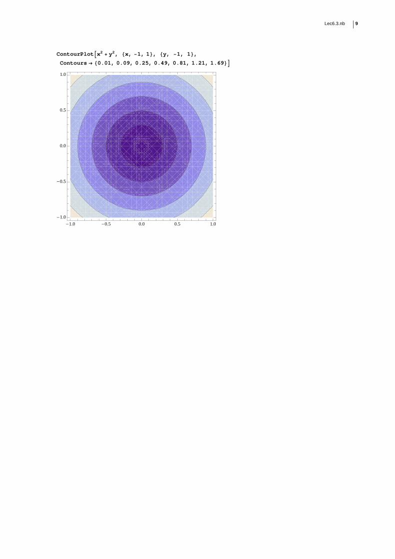
ContourPlotAx2 + y2, 8x, -1, 1<, 8y, -1, 1<,Contours ® 80.01, 0.09, 0.25, 0.49, 0.81, 1.21, 1.69<E

-1.0 -0.5 0.0 0.5 1.0

-1.0

-0.5

0.0

0.5

1.0

Lec6.3.nb 9

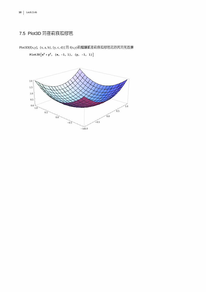
7.5 Plot3D でグラフを描く

Plot3D[f[x,y], {x, a, b}, {y, c, d}] で f(x,y)の３次元グラフを描くことができる。

Plot3DAx2 + y2, 8x, -1, 1<, 8y, -1, 1<E

-1.0

-0.5

0.0

0.5

1.0

-1.0

-0.5

0.0

0.5

1.00.0

0.5

1.0

1.5

2.0

10 Lec6.3.nb

7.6 ListPlot でグラフを描く

いくつかの数やシンボルをコンマで区切り、{ } で囲んだものをリストという。

numbers = 81, 3, 6, 10, -2, 0, 6<

81, 3, 6, 10, -2, 0, 6<

Length@numbersD

7

numbers@@2DD

3

numbers@@6DD

0

list1 = 8a, b, c<

8a, b, c<

list2 = 81, 2, 3<

81, 2, 3<

リストのリストというものを考えることもできる。

nestlist = 8list1, list2<

88a, b, c<, 81, 2, 3<<

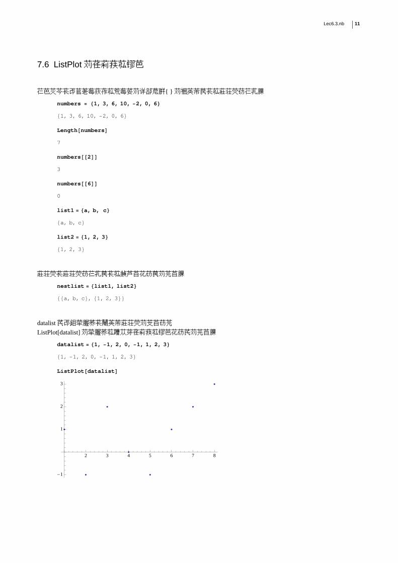
datalist が数値データの並んだリストであるとき

ListPlot[datalist] でデータを使ったグラフを描くことができる。

datalist = 81, -1, 2, 0, -1, 1, 2, 3<

81, -1, 2, 0, -1, 1, 2, 3<

ListPlot@datalistD

2 3 4 5 6 7 8

-1

1

2

3

Lec6.3.nb 11

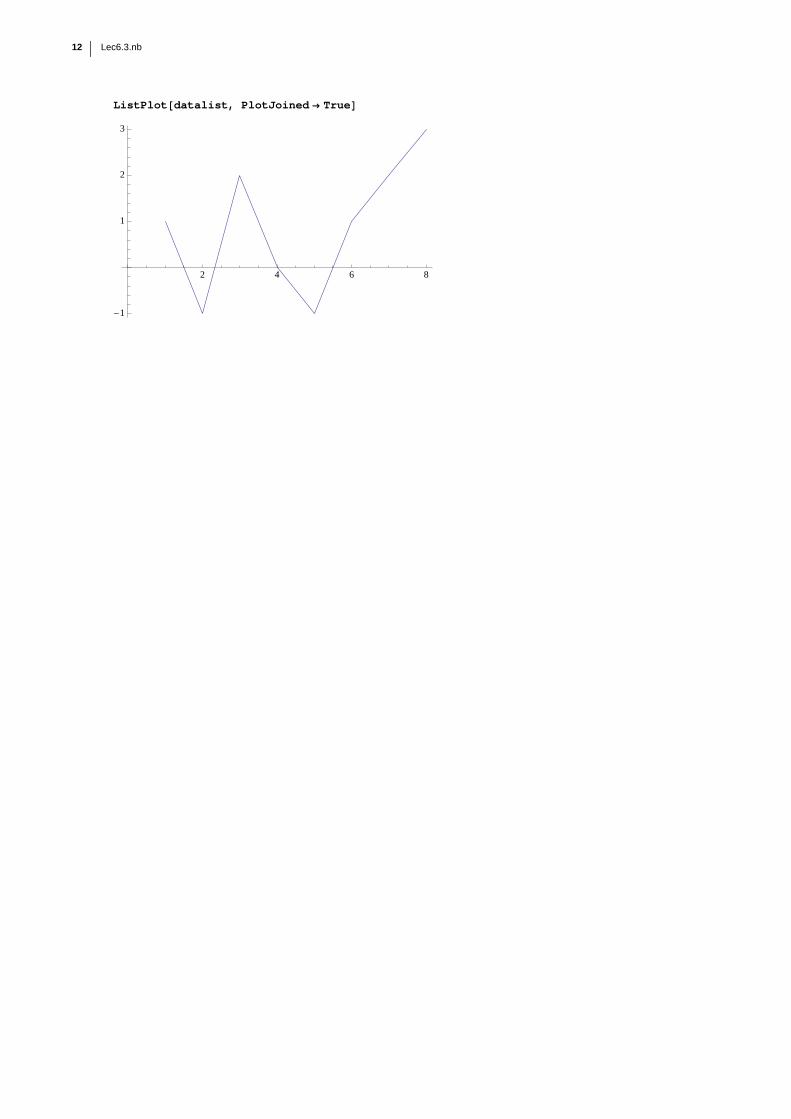
ListPlot@datalist, PlotJoined ® TrueD

2 4 6 8

-1

1

2

3

12 Lec6.3.nb

８. ドキュメントを作成するために

8.1 セルについて

Mathematica のノートブックは「セル」が集まってできている。

セル　®　右端の括弧で示される最小単位

セルの種類

Input : Mathematica にコマンドを与える（デフォルトで選択されている）

Output : Mathematica からの出力が表示される（入力セルとペアになっている）

Text Cell : 文書を書く

Title, Subtitle, Subsubtitle : タイトルなど

Section, Subsection, Subsubsection : 章立てなど

セルの種類を指定するには、「ウィンドウ」®「ツールバーの表示」によってツールバーを出して、左上のプル

ダウンメニューから指定するか、「書式」®「スタイル」から指定する（Alt + 番号）。

Lec6.3.nb 13