Embed Size (px)
Citation preview
Alma Mater Studiorum · Universita diBologna
FACOLTA DI SCIENZE MATEMATICHE, FISICHE E NATURALI
Corso di Laurea Magistrale in Matematica
A HOMOLOGICAL DEFINITION
OF THE
HOMFLY POLYNOMIAL
Tesi di Laurea in Topologia Algebrica
Relatore:
Chiar.mo Prof.
Massimo Ferri
Co-relatore
Chiar.mo Prof.
Christian Blanchet
Presentata da:
Roberto Castellini
II Sessione
Anno Accademico 2011/2012

Introduzione
La teoria dei nodi e la branca della topologia che studia il comportamento
di un cerchio, o di un’unione disgiunta di cerchi, chiamata link, nello spazio
R3. Per i risultati ottenuti nello studio di varieta di dimensione 3 e 4, la
teoria dei nodi e spesso considerata parte della topologia di dimensione bassa.
Problemi riguardanti i nodi emergono anche nella teoria della singolarita e
nella geometria simplettica. Notevoli sono anche le applicazioni ad altre
discipline scientifiche, in particolar modo la fisica e la biologia.
La nozione di equivalenza tra nodi e l’isotopia, che corrisponde a consi-
derare un nodo come un filo unidimensionale, flessibile ed elastico. Se pero
dimostrare che due nodi sono equivalenti corrisponde a trovare un’isotopia
tra i due, per provare la non equivalenza e necessario dimostrare che una tale
isotopia non possa esistere. E’ quindi necessario studiare delle caratteristi-
che geometriche invarianti per isotopia. I primi invarianti trovati erano pero
troppo difficili da calcolare.
Per questo motivo si studiano non tanto caratteristiche geometrico topo-
logiche dei nodi, ma piuttosto si cerca di utilizzare gli strumenti della topolo-
gia algebrica. Uno dei primi invarianti e stato il gruppo fondamentale del
nodo, definito come il gruppo fondamentale del complementare del nodo,
visto in R3 o, equivalentemente, in S3. Il primo invariante efficientemente
calcolabile e pero il polinomio di Alexander, sviluppato contemporaneamente
negli anni venti da Alexander e Reidemeister. Lo sviluppo della teoria si
concentro sullo studio delle proprieta del polinomio di Alexander, dandone
diverse interpretazioni (tra cui il calcolo di Fox), nonche sui legami con la
i

ii Introduzione
teoria della torsione di Reidemeister. Sempre tramite la teoria di Reidemei-
ster si ha un’interpretazione degli zeri del polinomio nell’ambito della teoria
della rappresentazione del gruppo fondamentale dei nodi.
Nel 1981 L. Kauffman caratterizza il polinomio di Alexander puramente
in termine combinatori. Considerando un nodo L, si focalizza su un incrocio
e chiama K+ il nodo in cui l’incrocio e ’positivo’ e K− il nodo con incrocio
’negativo’. Ottiene cosı la seguente relazione, detta relazione di Alexander-
Conway,
• ∆O(t) = 1
• ∆K+(t)−∆K−(t) = (t1/2 + t−1/2)∆K(t)
dove ∆K(t) e il polinomio di Alexander di un dato nodo K. Questa re-
lazione permette di calcolare in maniera induttiva il polinomio, dal momento
che qualsiasi nodo puo essere trasformato nel nodo banale con un numero
finito di cambi nel diagramma.
Nel 1984 Vaughan Jones, durante una ricerca sulla teoria delle algebre di
Von Neumann, scopre un nuovo polinomio per nodi orientati, il polinomio di
Jones. Questo polinomio e univocamente determinato dalle due condizioni
1. VO(t) = 1
2. tV K+(t)− t−1VK−(t) = (t1/2 + t−1/2)VK(t)
vedi [15].
La costruzione attraverso le relazioni 1 e 2 ha ispirato alcuni ricercatori
sulla possibilita di una possibile generalizzazione ad un polinomio in due
variabili. Nello stesso periodo, diversi autori hanno scoperto un nuovo poli-
nomio, o, meglio, differenti versioni isomorfe delle stesso polinomio, [12]. Il
nuovo invariante, il polinomio HOMFLY, prese il suo nome dalle iniziali dei
suoi 6 scopritori: J. Hoste, A. Ocneanu, K. Millett, P. Freyd, W.B.R. Licko-
rish, D. Yetter. Al momento, sono conosciuti tre polinomi associati ai nodi:
Introduzione iii
l’Alexander-Conway, quello di Jones e il polinomio HOMFLY, l’ultimo dei
quali contenente come casi particolari i primi due.
Nel 2001 Bigelow ha presentato una interpretazione geometrica del poli-
nomio di Jones, [2]. L’obiettivo di questa tesi e studiare una definizione omo-
logica del polinomio HOMFLY, sempre scoperta da Bigelow e pubblicata in
[4]. Questa e definita non sui nodi, ma sulle trecce. Il gruppo di trecce fu
introdotto da Emil Artin negli anni ’20 e presto emersero connessioni con la
teoria dei nodi. E’ infatti possibile ottenere link dalle trecce in una maniera
standard, con un’operazione chiamata chiusura. Per un teorema di Alexan-
der, e possibile ottenere ogni link come chiusura di un’opportuna treccia. Ve-
dremo quindi una definizione del polinomio HOMFLY in termini di chiusura
di trecce, piu esattamente con una differente chiusura, chiamata ’plat clo-
sure’, definita su trecce con un numero pari di corde. Questa costruzione e
dovuta a Birman, [5].
Vediamo ora brevemente gli argomenti trattati nei vari capitoli.
Nel primo capitolo sono presentati i risultati classici della teoria dei nodi.
Il primo paragrafo e dedicato a illustrare le definizioni fondamentali della
teoria dei nodi e alla costruzione del primo invariante algebrico, il gruppo del
nodo. Nel secondo paragrafo definiamo il polinomio di Alexander in quattro
maniere diverse, attraverso spazi di ricoprimento, superfici di Seifert, calcolo
di Fox e relazioni del tipo 1 e 2, dette relazioni ’skein’. Nel terzo paragrafo e
introdotto il polinomio di Jones.
Il secondo capitolo e completamente dedicato alle trecce. Nel primo para-
grafo introduciamo differenti definizioni equivalenti del gruppo di trecce. Nel
paragrafo successivo sono studiate alcune delle sue proprieta. Il terzo para-
grafo e dedicato a investigare l’equivalenza tra trecce e link. Nell’ultimo
paragrafo sono presentati alcuni risultati relativi alla rappresentazione del
gruppo lineare, per arrivare a citare il teorema di linearita del gruppo di
trecce.
Nel terzo capitolo ci occupiamo del risultato principale della tesi, la
costruzione di una definizione omologica del polinomio HOMFLY. Nel primo

iv Introduzione
paragrafo e definito il polinomio. Nel secondo paragrafo viene presentata la
costruzione geometrica utilizzata nei paragrafi successivi. Nei due successivi,
e definito un invariante sulle trecce, insieme a una spiegazione del suo signifi-
cato topologico. Nell’ultimo paragrafo dimostriamo il teorema fondamentale,
l’equivalenza dell’invariante definito sulle trecce e del polinomio HOMFLY.
Introduction
Knot theory is the branch of topology which studies the behaviour of a
circle, or of a disjoint union of circles, a link, in the space R3. Due to the
results concerning topological manifolds of dimension 3 and 4, knot theory is
often considered as part of low dimensional topology. Problems about knots
also emerge in singularity theory and in simplectic geometry. Remarkable are
also the applications in other scientific disciplines, as physics and biology.
The notion of knot equivalence is known as isotopy, which consists in con-
sidering a knot as a unidimensional thread, flexible and elastic. While proving
two knots’ equivalence is proving the existence of a particular isotopy, prov-
ing that two knots are not equivalent consists in showing the impossibility
of such an isotopy. It is thus necessart to study geometric features which
are invariant for isotopy. The first invariants found were very difficult to
compute.
This is the reason we do not study the geometrical-topological knot be-
haviour, but rather we try to use algebraic topology tools. One of the first
invariants was the knot fundamental group, defined as the fundamental group
of the knot complementary, seen in R3 or, equivalently, in S3. The first in-
variant effectively computable is the Alexander polynomial, developed at the
same time in the ’20 by Alexander and Reidemeister. Further developments
of the theory focused on the study of these polynomial proprieties, giving
different interpretations of it (like Fox calculus), as well as on the bonds
to Reidemeister torsion theory. Thanks moreover to Reidemeister’s theory
we have an interpretation of the zeros of the polynomial in the theory of
v
vi Introduction
representation of the knot fundamental group.
In 1981 L. Kauffman defines Alexander’s polynomial in a purely combi-
natorial way. Taking a knot K, we focus on a crossing and we call K+ the
knot where this crossing is ’positive’ and K− the knot where this crossing
is ’negative’. We obtain then the following relation, the Alexander-Conway
relation,
• ∆O(t) = 1
• ∆K+(t)−∆K−(t) = (t1/2 + t−1/2)∆K(t)
where ∆K(t) is the Alexander’s polynomial of a given know K. This rela-
tion allows to compute in an inductive way the polynomial, since every knot
can be transformed in the trivial knot with a finite number of transformations
of the crossing type in the diagram.
In 1984 Vaughan Jones, during a research on Von Neumann algebras,
found a new oriented knot polynomial, the Jones polynomial. This polyno-
mial is uniquely determined by the two conditions
1. VO(t) = 1
2. tV K+(t)− t−1VK−(t) = (t1/2 + t−1/2)VK(t)
see [15].
The construction via relations 1 and 2 pointed towards the possibility
of generalisation in two indeterminate. At the same time, different authors
discovered a new polynomial, or rather isomorphic versions of the same poly-
nomial, [12]. This new invariant, the HOMFLY polynomial, took its name
from the initials of the 6 discoverers: J. Hoste, A. Ocneanu, K. Millett, P.
Freyd, W.B.R. Lickorish, D. Yetter. At present, there are three main known
knot polynomials: the Alexander-Conway, the Jones and the HOMFLY poly-
nomials, the last one containing as particular cases the first two.
In 2001 Bigelow presented a geometric interpretation of the Jones polyno-
mial, see [2]. In this thesis we studied a homological definition of the HOM-
FLY polynomial, discovered as well by Bigelow, see [4]. This construction
Introduction vii
was not defined on the basis of knots, but braids. These were introduced by
Emil Artin in the 1920s. It is possible to pass in a standard way from braids
to links with an operation called closure. Through a theorem by Alexander,
it is possible to take each link as a closure of an opportune braid. There
is a definition of the HOMFLY polynomial in terms of closures of braids,
more exactly as plat closures of braids with an even number of strings. This
construction is due to Birman.
Now we briefly summarise the contents of this thesis.
In the first chapter we give the classic results of knot theory. The first
section is dedicated to illustrate the fundamental definitions of knot theory
and of the first algebraic invariant, the knot group. In the second section we
define the Alexander polynomial in four different ways, via covering spaces,
via Seifert surfaces, via Fox calculus and via skein relations. In the third
section we introduce the Jones polynomial.
The second chapter is dedicated to braids. In the first section we introduce
different equivalent definitions of the braid group. In the following section,
we study some of its proprieties. The third section is dedicated to investigate
the equivalence between braids and links. In the last section we see some
linear representations of braid groups, stating the linearity of braid groups.
In the third chapter we prove the main statement of this work, the build-
ing of a homological definition of the Homfly polynomial. In the first section
we define the polynomial. The fundamental geometric constructions are pre-
sented in the second section. In the following two sections, we define an
invariant on braids and we find a topological meaning for this invariant. In
the last section we prove the fundamental theorem, the equivalence of the
invariant on braids and the HOMFLY polynomial.

Contents
Introduzione i
Introduction v
1 Knots 1
1.1 Knots and fundamental group . . . . . . . . . . . . . . . . . . 1
1.1.1 Definitions . . . . . . . . . . . . . . . . . . . . . . . . . 1
1.1.2 Knot groups . . . . . . . . . . . . . . . . . . . . . . . . 4
1.1.3 Knots classification . . . . . . . . . . . . . . . . . . . . 8
1.1.4 Some examples . . . . . . . . . . . . . . . . . . . . . . 9
1.2 The Alexander-Conway polynomial . . . . . . . . . . . . . . . 12
1.2.1 The Alexander module . . . . . . . . . . . . . . . . . . 12
1.2.2 Seifert surfaces . . . . . . . . . . . . . . . . . . . . . . 17
1.2.3 Fox differential calculus . . . . . . . . . . . . . . . . . 23
1.2.4 Fox differential calculus for knots groups . . . . . . . . 27
1.2.5 The Alexander-Conway polynomial . . . . . . . . . . . 31
1.3 The Jones polynomial . . . . . . . . . . . . . . . . . . . . . . 34
1.3.1 Definition by Kaufmann brackets . . . . . . . . . . . . 34
1.3.2 Definition by skein relations . . . . . . . . . . . . . . . 38
2 Braid groups 41
2.1 Some equivalent definitions . . . . . . . . . . . . . . . . . . . . 41
2.1.1 Configuration spaces . . . . . . . . . . . . . . . . . . . 41
2.1.2 Diagrams . . . . . . . . . . . . . . . . . . . . . . . . . 42
ix
x Introduction
2.1.3 Presentation . . . . . . . . . . . . . . . . . . . . . . . . 45
2.1.4 Mapping class groups . . . . . . . . . . . . . . . . . . . 48
2.2 Proprieties . . . . . . . . . . . . . . . . . . . . . . . . . . . . . 52
2.2.1 Pure braid group . . . . . . . . . . . . . . . . . . . . . 52
2.2.2 The center of Bn . . . . . . . . . . . . . . . . . . . . . 57
2.2.3 Homotopy groups . . . . . . . . . . . . . . . . . . . . . 60
2.3 Representation of links by braids . . . . . . . . . . . . . . . . 61
2.3.1 Construction of links by braids . . . . . . . . . . . . . 61
2.3.2 Alexander’s theorem . . . . . . . . . . . . . . . . . . . 63
2.3.3 Markov theorem . . . . . . . . . . . . . . . . . . . . . 66
2.4 Representations of braid groups . . . . . . . . . . . . . . . . . 68
2.4.1 The Burau representation . . . . . . . . . . . . . . . . 68
2.4.2 A homological description of the Burau representation 70
2.4.3 Krammer-Bigelow-Lawrence representation . . . . . . . 72
3 The HOMFLY polynomial 75
3.1 Construction of the polynomial . . . . . . . . . . . . . . . . . 75
3.1.1 Definition . . . . . . . . . . . . . . . . . . . . . . . . . 75
3.1.2 Construction by Hecke algebra . . . . . . . . . . . . . . 77
3.2 The configuration space . . . . . . . . . . . . . . . . . . . . . 82
3.2.1 Construction of the space . . . . . . . . . . . . . . . . 82
3.2.2 A torus and a ball . . . . . . . . . . . . . . . . . . . . 85
3.2.3 Construction in the case N=2 . . . . . . . . . . . . . . 85
3.2.4 Construction for general values of n . . . . . . . . . . . 87
3.3 The invariant on braids . . . . . . . . . . . . . . . . . . . . . . 90
3.3.1 Definition . . . . . . . . . . . . . . . . . . . . . . . . . 90
3.4 A homological definition . . . . . . . . . . . . . . . . . . . . . 91
3.4.1 Barcodes . . . . . . . . . . . . . . . . . . . . . . . . . . 92
3.4.2 Basis for the homology . . . . . . . . . . . . . . . . . . 94
3.4.3 The image of T . . . . . . . . . . . . . . . . . . . . . . 95
3.4.4 Partial bar codes . . . . . . . . . . . . . . . . . . . . . 97
3.5 The equivalence of the two invariants . . . . . . . . . . . . . . 99
INDEX xi
3.5.1 Invariance under movements . . . . . . . . . . . . . . . 99
3.5.2 The Markov Birman stabilization . . . . . . . . . . . . 103
3.5.3 Equivalence with the HOMFLY polynomial . . . . . . 106
Appendix
A Local Coefficients via Bundles of Groups 111
Bibliography 115

Chapter 1
Knots
1.1 Knots and fundamental group
1.1.1 Definitions
Definition 1. A knot K is a smooth sub-variety in S3 diffeomorphic to the
circle S1. If S1 is oriented, the diffeomorphism preserves the orientation and
we say that the knot is oriented.
Example 1. The trivial knot:
(x, y, z) ∈ S3| x2 + y2 = 1, z = 0
Example 2. Knots lying on the surface of an unknotted torus in S3 are
called torus knots. Each knot torus can be specified by two coprime integers
p and q, where p is the number of windings along the longitude and q is the
number of windings along the meridian of the torus T 2.
Let us see an example of parametrization. The curve γp,q : S1 → R3 is
given by
θ 7→ (cos(pθ)
1− sin(qθ),
sin(pθ)
1− sin(qθ),
cos(qθ)
1− sin(qθ)).
Definition 2. A n-component link L is a smooth subvariety in S3 diffeomor-
phic to a disjoint union on n circles S1.
1
2 1. Knots
Definition 3. An isotopy between two knots K and K ′ in S3 is a map
h : [0, 1]× S3 → S3
(t, x) 7→ ht(x)
such that:
• h0 = IdS3
• ∀t ht is a diffeomorphism
• K ′ = h1(K)
Two knots K and K ′ are isotopic if and only if there is an isotopy h
between them.
Remark 1. The relation ’K is isotopic to K ′’ is an equivalence relation.
Definition 4. The knot obtained from K by inverting its orientation is called
the inverted knot and it is denoted by −K.
The mirrored knot of K is obtained by a reflection of K in a plane and
it is denoted by K∗.
A knot K is called invertible is K = −K up to isotopy and amphicheiral
if K = K∗ up to isotopy.
It is possible to define the notion of knot and isotopy also in the piecewise
linear category, rather than in the smooth category. It turns out that in three
dimensions, the smooth category and the piecewise category are the same,
so there is no substantial difference between the two definitions.
Definition 5. A knot diagram is a regular projection, i.e. it is such that
multiple points are double points with different tangent vectors, of a circle
S1 in the oriented plane R2, with an over-under information for every double
point.
Remark 2. The set of double points is a discrete set.
1.1 Knots and fundamental group 3
Every diagram can be associated to a isotopy class of knots in S3. The
diagram is immersed in R2 × 0 and to every crossing just push the under
point in a smooth way so that it lies in the plane z = −ε, ε > 0.
Proposition 1.1.1. The set of regular projections is open and dense in the
space of all projections.
A proof of this proposition in PL situation can be find in [Bur85].
It follows from the proposition:
Theorem 1.1.2. Every knot in S3 is isotopic to a knot with regular projec-
tion in R2. Every knot can be defined as a diagram, up to isotopy.
Now we want to see how the condition of isotopy equivalence can be
expressed in terms of diagrams.
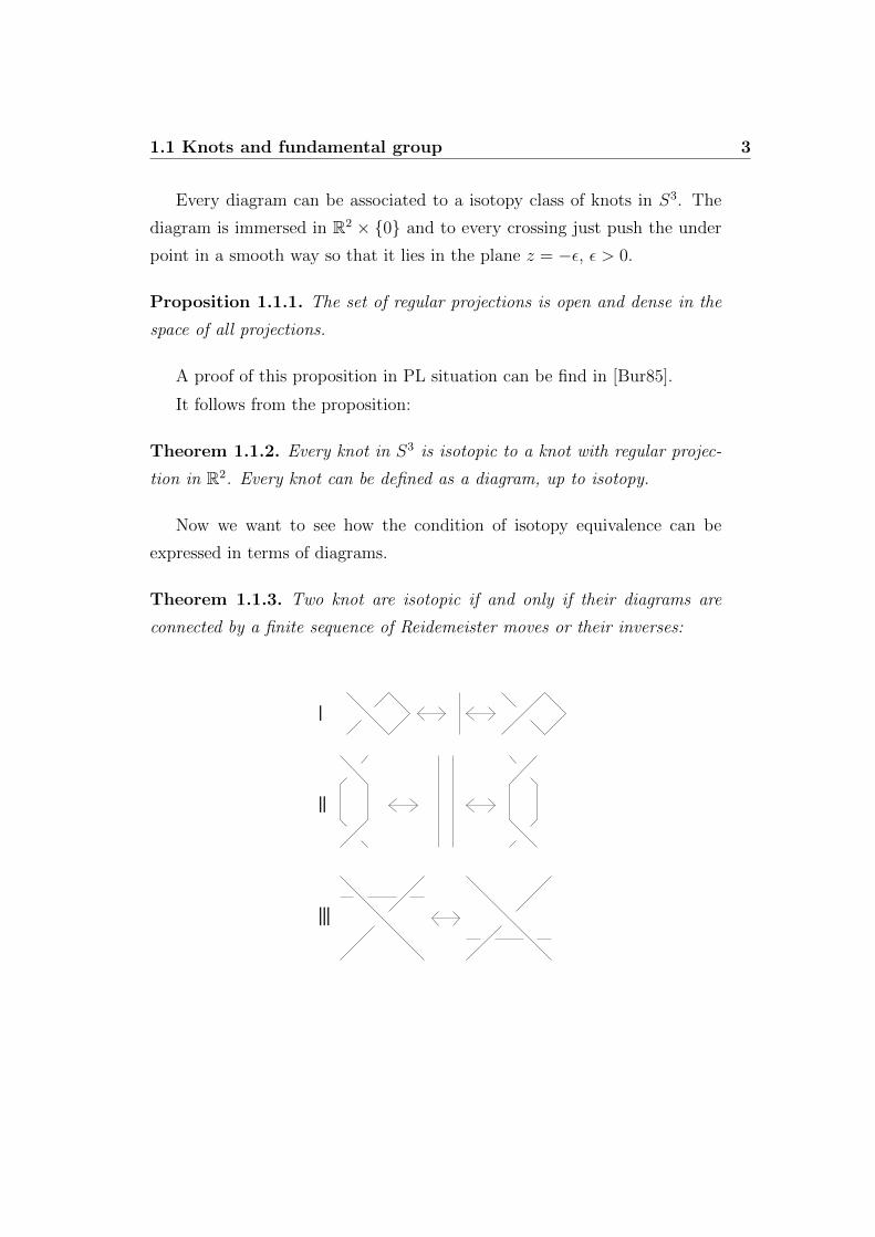
Theorem 1.1.3. Two knot are isotopic if and only if their diagrams are
connected by a finite sequence of Reidemeister moves or their inverses:
I
II
III
4 1. Knots
A proof can be find, in the PL case, in [8].
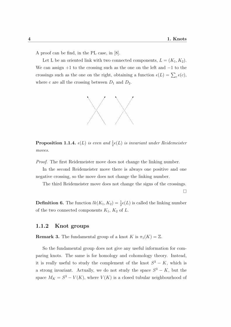
Let L be an oriented link with two connected components, L = (K1, K2).
We can assign +1 to the crossing such as the one on the left and −1 to the
crossings such as the one on the right, obtaining a function ε(L) =∑
c ε(c),
where c are all the crossing between D1 and D2.
Proposition 1.1.4. ε(L) is even and 12ε(L) is invariant under Reidemeister
moves.
Proof. The first Reidemeister move does not change the linking number.
In the second Reidemeister move there is always one positive and one
negative crossing, so the move does not change the linking number.
The third Reidemeister move does not change the signs of the crossings.
Definition 6. The function lk(K1, K2) = 12ε(L) is called the linking number
of the two connected components K1, K2 of L.
1.1.2 Knot groups
Remark 3. The fundamental group of a knot K is π1(K) = Z.
So the fundamental group does not give any useful information for com-
paring knots. The same is for homology and cohomology theory. Instead,
it is really useful to study the complement of the knot S3 − K, which is
a strong invariant. Actually, we do not study the space S3 − K, but the
space MK = S3 − V (K), where V (K) is a closed tubular neighbourhood of
1.1 Knots and fundamental group 5
the knot K. They have the same homology, because they are homotopically
equivalent, but MK is a compact 3-manifold with boundary.
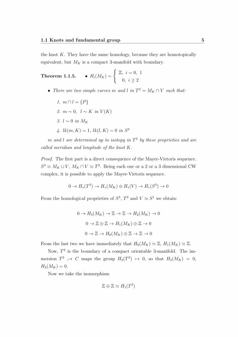
Theorem 1.1.5. • Hi(MK) =
Z, i = 0, 1
0, i ≥ 2
• There are two simple curves m and l in T 2 = MK ∩ V such that:
1. m ∩ l = P
2. m ∼ 0, l ∼ K in V (K)
3. l ∼ 0 in MK
4. lk(m,K) = 1, lk(l,K) = 0 in S3
m and l are determined up to isotopy in T 2 by these proprieties and are
called meridian and longitude of the knot K.
Proof. The first part is a direct consequence of the Mayer-Vietoris sequence.
S3 'MK ∪ V , MK ∩ V ' T 2. Being each one or a 2 or a 3 dimensional CW
complex, it is possible to apply the Mayer-Vietoris sequence.
0→ H∗(T2)→ H∗(MK)⊕H∗(V )→ H∗(S
3)→ 0
From the homological proprieties of S3, T 2 and V ' S1 we obtain:
0→ H3(MK)→ Z→ Z→ H2(MK)→ 0
0→ Z⊕ Z→ H1(MK)⊕ Z→ 0
0→ Z→ H0(MK)⊕ Z→ Z→ 0
From the last two we have immediately that H0(MK) ' Z, H1(MK) ' Z.
Now, T 2 is the boundary of a compact orientable 3-manifold. The im-
mersion T 2 → C maps the group H2(T 2) 7→ 0, so that H2(MK) = 0,
H3(MK) = 0.
Now we take the isomorphism
Z⊕ Z ' H1(T 2)
6 1. Knots
in the Mayer-Vietoris sequence. The generators ofH1(V ) ' Z andH1(MK) 'Z are determined up to the inverse. We can choose l, a representative of the
homology class of K, as a generator of H1(V ) with the condition that l be
homologous to 0 in H1(MK). So l is unique up to isotopy in T 2. Equiva-
lently, a generator of H1(MK) can be represented by a curve m in T 2 that
is homologous to 0 in V . With this choices of l and m we obtain a system
of generators of H1(T 2) ' Z⊕ Z. We can also assume that m is simple and
intersects l in one point, see [23].
The linking number proprieties follow from the construction.
The most important invariant of a knot (and of a link) is the so called
knot group (link group).
Definition 7. The group π1(ML), where L is a link, is called the link group.
Remark 4. Generally, we take as basepoint the point (0, i), viewing S3 as
a subspace of C2.
Remark 5. The knot group is independent of the choice of the orientation,
but the orientation defines uniquely the generators.
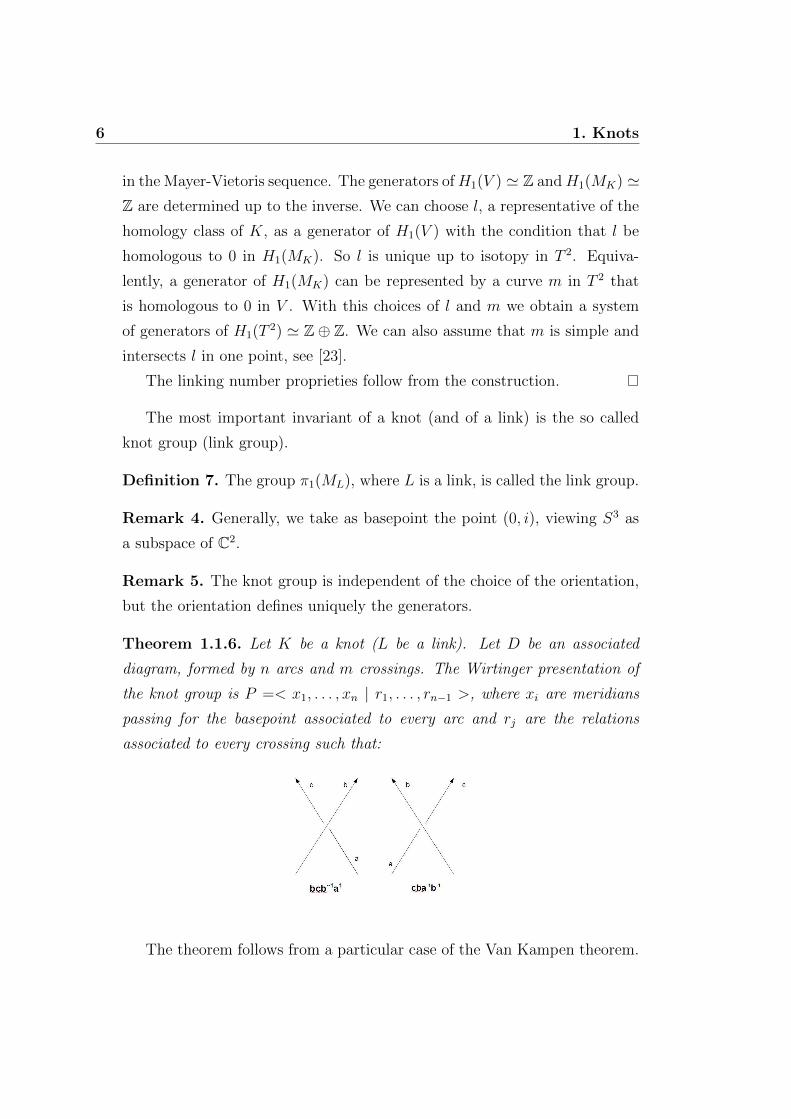
Theorem 1.1.6. Let K be a knot (L be a link). Let D be an associated
diagram, formed by n arcs and m crossings. The Wirtinger presentation of
the knot group is P =< x1, . . . , xn | r1, . . . , rn−1 >, where xi are meridians
passing for the basepoint associated to every arc and rj are the relations
associated to every crossing such that:
The theorem follows from a particular case of the Van Kampen theorem.
1.1 Knots and fundamental group 7
Theorem 1.1.7. Let (X, x0) be a pointed topological space, union of two
open sets U1 and U2 such that U1∩U2 is arc-connected and x0 ∈ U1∩U2. Let
us also suppose that U2 is simply connected. Let i and j be the applications:
i : U1 ∩ U2 → U1
j : U1 → X
Then the application
j# : π1(U1, x0)→ π1(X, x0)
induces an isomorphism
π1(U1, x0)
i#(π1(U1 ∩ U2, x0))N' π1(X, x0)
Proof. A proof can we found in [14].
Now we can prove the main theorem on the Wirtinger presentation.
Proof. We can take the knot K as being immersed in R3. Let XK be XK =
R3 −K. We take two sets U1, U2 ⊂ XK such that:
U1 = (z ≥ −ε ∪ ∞) ∩XK
U2 = (z ≤ −ε ∪ ∞) ∩XK
where, up to homeomorphism, we can take the basepoint x0 to be∞. Again
up to homeomorphism, we can choose ∞ such that ∞ /∈ K.
We can not apply directly theorem 1.1.7 because the intersection of the
two sets is closed. But in this situation it is not a big problem, because
3−manifolds can be always seen as CW-complexes and theorem 1.1.7 is true
also with closed sets.
Now we have a sequence
U1 ∩ U2j→ U1
i→ XK
8 1. Knots
Applying the Van Kampen theorem, i# induces an isomorphism
π1(U1,∞)
j#(π1(U1 ∩ U2))N∼→ π1(XK ,∞)
Now we can take U1 as a 3-dimensional disk, and so U1 becomes home-
omorphic to a 3-dimensional disk without some arcs. By recursion, we can
apply many times the Van Kampen theorem. The group π1(U1,∞) is a free
group generated by the meridian associated to the arc. Instead U1 ∩ U2 is a
sphere minus n− 1 arcs. It remains to study j#.
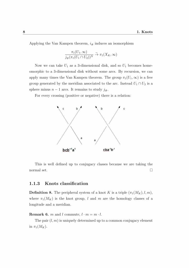
For every crossing (positive or negative) there is a relation:
This is well defined up to conjugacy classes because we are taking the
normal set.
1.1.3 Knots classification
Definition 8. The peripheral system of a knot K is a triple (π1(MK), l,m),
where π1(MK) is the knot group, l and m are the homology classes of a
longitude and a meridian.
Remark 6. m and l commute, l ·m = m · l.The pair (l,m) is uniquely determined up to a common conjugacy element
in π1(MK).
1.1 Knots and fundamental group 9
Theorem 1.1.8. (Waldhausen)
Two knots K1 and K2 in S3 with peripheral systems (π1(MK1), l1,m1),
(π1(MK2), l2,m2) are equal if and only if there is an isomorphism ϕ : π1(MK1)→π1(MK2) such that ϕ(l1) = l2 and ϕ(m1) = m2.
Proof. A proof can be found in [8].
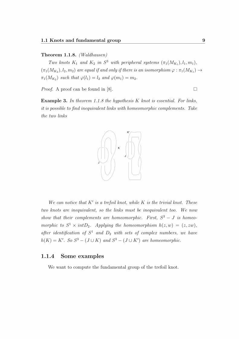
Example 3. In theorem 1.1.8 the hypothesis K knot is essential. For links,
it is possible to find inequivalent links with homeomorphic complements. Take
the two links
J
K
J
K'
We can notice that K ′ is a trefoil knot, while K is the trivial knot. These
two knots are inequivalent, so the links must be inequivalent too. We now
show that their complements are homeomorphic. First, S3 − J is homeo-
morphic to S1 × intD2. Applying the homeomorphism h(z, w) = (z, zw),
after identification of S1 and D2 with sets of complex numbers, we have
h(K) = K ′. So S3 − (J ∪K) and S3 − (J ∪K ′) are homeomorphic.
1.1.4 Some examples
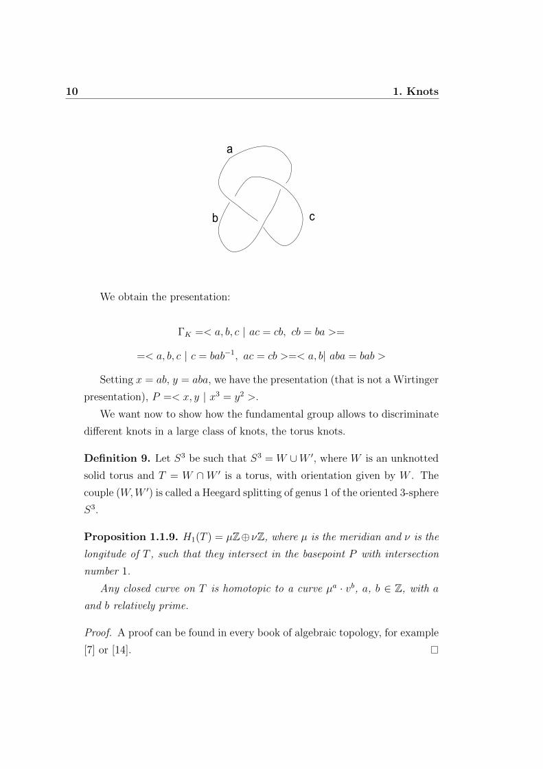
We want to compute the fundamental group of the trefoil knot.
10 1. Knots
a
b c
We obtain the presentation:
ΓK =< a, b, c | ac = cb, cb = ba >=
=< a, b, c | c = bab−1, ac = cb >=< a, b| aba = bab >
Setting x = ab, y = aba, we have the presentation (that is not a Wirtinger
presentation), P =< x, y | x3 = y2 >.
We want now to show how the fundamental group allows to discriminate
different knots in a large class of knots, the torus knots.
Definition 9. Let S3 be such that S3 = W ∪W ′, where W is an unknotted
solid torus and T = W ∩W ′ is a torus, with orientation given by W . The
couple (W,W ′) is called a Heegard splitting of genus 1 of the oriented 3-sphere
S3.
Proposition 1.1.9. H1(T ) = µZ⊕νZ, where µ is the meridian and ν is the
longitude of T , such that they intersect in the basepoint P with intersection
number 1.
Any closed curve on T is homotopic to a curve µa · vb, a, b ∈ Z, with a
and b relatively prime.
Proof. A proof can be found in every book of algebraic topology, for example
[7] or [14].
1.1 Knots and fundamental group 11
Definition 10. Let (W,W ′) be a Heegard splitting of genus 1 of S3. If K is
a simple closed curve on F with intersection numbers p, q with ν and µ, |p|,|q| ≥ 2, then K is called the torus knot K(p, q).
Remark 7.
K(−p,−q) = −K(p, q)
K(p,−q) = K∗(p, q)
K(p, q) = K(−p,−q) = K(q, p)
Proposition 1.1.10. A presentation of the group Γ(p, q) of the torus knot
K(p, q) is
Γ(p, q) =< u, v | upv−q >
where u and v represents µ and ν. It has the following proprieties:
1. The centre is < ua >' Z.
2. m = urvs, l = upm−pq, ps+qr = 1, m and l are meridian and longitude
of K(p, q) for a suitable basepoint P .
3. K(p, q) and K(p′, q′) have isomorphic groups if and only if |p| = |p′|and |q| = |q′| or |p| = |q′| and |q| = |p′|.
Proof. It follows from standard results in Heegard splitting, see [8].
Theorem 1.1.11. K(p, q) = K(p′, q′) if and only if (p′, q′) is equal to: (p, q),
(q, p), (−p,−q) or (−q,−p). Also, torus knots are invertible, but not am-
phicheiral.
Proof. Sufficiency has been proven in the previous proposition. Suppose
now K(p, q) = K(p′, q′). The centre Z(Γ) is a characteristic subgroup, so
Γ(p, q)/Z is a knot invariant. Also, the integers |p|, |q| are invariants of
Z|p| ∗ Z|q| and they are the orders of maximal finite subgroups of Z|p| ∗ Zq,which are not conjugate. This proves the first part of the statement.
12 1. Knots
Let now p, q be such that p, q > 0. There is an isomorphism ϕ :
Γ(p, q) → Γ(p′, q′) such that it maps the peripheral system (Γ(p, q),m, l)
in (Γ(p′, q′),m′, l′):
m′ = ϕ(urvs) = u′r′v′s′
l′ = ϕ(up(crvs)−pq) = u′p(u′r′v′d′)−pq
where ps+ qr = ps′ − qr′ = 1, so that s′ = s+ jq and r′ = r + jp, for j ∈ Z.
The isomorphism ϕ maps the centre Z(Γ(p, q)) in Z(Γ(p′, q′)), so that
ϕ(up) = (u′p)ε, ε = ±1. We have
u′p(u′r′v′s′)pq = ϕ(up(urvs)−pq) = ϕ(up)ϕ(urvs)−pq = (u′p)ε(u′r
′v′s′)−pq
and so (u′p)1−ε = (u′r′v′s′)−2pq, that is impossible. In fact, the homomorphism
Γ(p′, q′) → Γ(p′, q′)/Z(Γ(p′, q′)) maps the terms on the left to 1, while the
term on the right represents a non-trivial element.
1.2 The Alexander-Conway polynomial
1.2.1 The Alexander module
Definition 11. The infinite cyclic cover of a knot K is the regular cover XK
of the complement of the knot K, associated to the morphism:
h : π1(Xk,∞)→ H1(XK ,Z)
Let us give a constructive definition of the space. Let Ω(XK ,∞, x) be the
space of all paths from ∞ to the point x in XK . By the theory of covering
spaces, XK is defined as
(x, γ), x ∈ XK , γ ∈ Ω(XK ,∞, x)/ ∼
where ∼ is the relation:
(x, γ) ∼ (x, γ′)⇔ x = x′, h[γ′γ−1] = 0
1.2 The Alexander-Conway polynomial 13
The group π1(XK ,∞) acts on XK via the application h, that factorises
by the quotient of H1(XK ,Z) ' Z. Let t be the generator of H1(XK). t
acts by a transformation t : XK → XK . So the transformations group of the
covering space is < t >, which acts on C∗(XK) by translation. More, it acts
on H∗(XK) and this action extends to the group ring Z[< t >] = Z[t±].
Definition 12. The Z[t±]-module H1(XK ,Z) is called the Alexander module
of the knot K.
Remark 8. H1(XK ;Z) is independent of the orientation of K, but the action
of Z[t±] is not. Changing the orientation exchanges t and t−1.
Definition 13. Let K be a knot and D an associated diagram. Let F be
the set of the connected bounded components of R2 −D. For every X ∈ Fwe can define
γX : [0, 1]→ R3
where R3 = R3 ∪∞, such that
γX(t) = (xX , yX , tan(π
2(2t− 1)))
The curve γX is called a Seifert generator.
Proposition 1.2.1. The laces γX generate π1(XK).
Proof. As in the proof of the Wirtinger presentation of the knot group, it is
sufficient to apply the Van Kampen theorem to appropriate subsets.
Remark 9. If K ′ is a knot, K ′ ∈ S3, then [K ′] ∈ H1(MK). We denote
I(K ′) = lk(K ′, K). If lk(K ′, K) = 0, [K ′] = 0 ∈ H1(MK).
γX can be seen as a knot in MK , so by remark 9 γX ∈ H1(MK).
Remark 10. The action of the lace γX is
[γX ].∞ = tI(γX).∞
14 1. Knots
Remark 11. For every face X, γX is a path from ∞ to tI(γX).∞.
We can now prove the main theorem about the presentation of the Alexan-
der module.
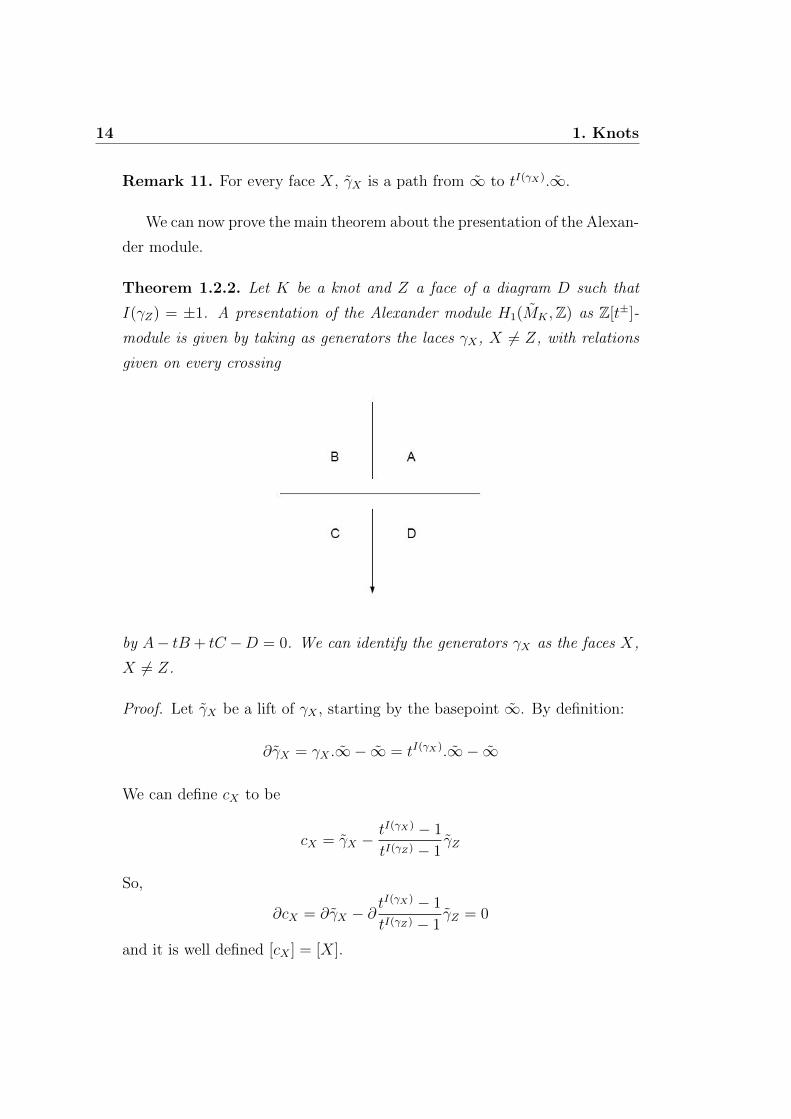
Theorem 1.2.2. Let K be a knot and Z a face of a diagram D such that
I(γZ) = ±1. A presentation of the Alexander module H1(MK ,Z) as Z[t±]-
module is given by taking as generators the laces γX , X 6= Z, with relations
given on every crossing
by A− tB + tC −D = 0. We can identify the generators γX as the faces X,
X 6= Z.
Proof. Let γX be a lift of γX , starting by the basepoint ∞. By definition:
∂γX = γX .∞ − ∞ = tI(γX).∞ − ∞
We can define cX to be
cX = γX −tI(γX) − 1
tI(γZ) − 1γZ
So,
∂cX = ∂γX − ∂tI(γX) − 1
tI(γZ) − 1γZ = 0
and it is well defined [cX ] = [X].
1.2 The Alexander-Conway polynomial 15
We want to apply the Mayer Vietoris sequence to the sets
V1 = MK −⋃
c crossings
(xc, yc)× [−ε, 0]
V2 =⋃
c crossings
Dr((xc, yc),ε
2)
We have V1 ∪ V2 'MK .
Let V1 and V2 be the images of the two sets in MK . If we take X1K =⋃
X∈F γX → V1, we obtain a homotopy equivalence H1(X1K)
∼→ H1(V1). As
a Z[t±]-module the cellular complex is free with basis ∞ at degree 0, γX
at degree 1. We also have a definition for the boundary operator, so we
can compute the homology. We obtain that H1(V1) is free on Z[t±] with
basis cX, X 6= Z. Now we want to study V2. We have that V2 ' D2, so
V2 ' V2 × Z. Then H∗(V2) = 0 for every ∗ ≥ 1.
We also have that V1 ∩ V2 ' ∂V2 × Z, so that we have, for every crossing
c, S1 × Z. Let lc be
lc = S1r ((xc, yc),−
ε
2)× Z
Then the lace lc ∈ V1 is homologous to
˜γAγBγCγD
We have the following proprieties:
1. uv = u(uv)
2. uu = u(uu)
3. u = uu
We can also write u = t−I(u)u
˜γAγBγCγD = γAtI(γA)−I(γB)γBt
I(γA)−I(γB)γCtI(γA)−I(γB)−I(γC)+I(γD)γD

16 1. Knots
Applying I(γA) = I(γB) + 1, I(γC) = I(γD) − 1 and writing in additive
notation we obtain
γA − tγB + tγC − γD
Example 1. Let us calculate the Alexander module for the trefoil knot.
A
B
CD3
1
2
I(γD) = ±1, depending on the orientation, so we can take D = Z. Now
we have for each crossing:
1. −A+B = 0
2. −tA+B − C = 0
3. B − tC = 0
We obtain then a presentation:1 −t 0
−1 1 1
0 −1 −t
Definition 14. The Alexander polynomial ∆K(t) is defined as the determi-
nant of the presentation matrix, modulo ±t±k.
1.2 The Alexander-Conway polynomial 17
Remark 12. Usually, it is written P.
= Q for an equality modulo ±t±k of
two polynomials P and Q in Z[t±1].
Example 2. Using the matrix presentation computed above, we find that
the Alexander polynomial for the trefoil know is
∆K(t) = t2 − t+ 1.
= 1− (t+ t−1)
1.2.2 Seifert surfaces
Proposition 1.2.3. A simple closed curve K ⊂ S3 is the boundary of an
orientable surface Σ, embedded in S3. Σ is called a Seifert surface.
Proof. A proof can be found in [8].
Definition 15. Suppose that M is a surface and that there is a solid cylinder
D2×[0, 1] such that (D2×[0, 1])∩F = 0, 1×D2, respecting the orientation.
Let M ′ be such that M ′ = ((M − 0, 1)×D2) ∪ [0, 1]× ∂D2. M ′ is said to
be obtained from M by surgery along the arc [0, 1]× 0.
Two surfaces M and N are said to be tube equivalent if one is obtained
from the other by surgery along the arc [0, 1]× 0.
Theorem 1.2.4. Suppose that Σ and Σ′ are two Seifert surfaces for an ori-
ented link L in S3. Then there is a sequence of Seifert surfaces Σ1,Σ2, . . . ,Σnwith Σ1 = Σ and Σn = Σ′, such that, for every i, Σi and Σi−1 are tube-
equivalents.
Proof. A proof can be found in [17].
We will now use the Seifert surfaces to give a different interpretation of
the Alexander polynomial. The Seifert surfaces are connected compact and
oriented surfaces, then they are completely classified by their genus g.
Proposition 1.2.5. Let K be an oriented knot, Σ a Seifert Surface and K ′
a knot transversal to S. Then
lk(K,K ′) = I(Σ ∩K ′)
18 1. Knots
where I(Σ, K ′) is the algebraic intersection.
Proof. We write the exact sequence:
H2(S3)→ H2(S3, VK)→ H1(VK)→ H1(S3)
For the homological proprieties of S3, H1(S3) = H2(S3) = 0, so there is
an isomorphism between the two middle terms. For homotopy equivalence
H1(VK) ' H1(K). We have now:
H2(S3, VK) ' H2(S3−V K , ∂(S3−
V K)) ' H1(S3 − VK)
where the first equivalence is given by excision and the second by Poincare
duality.
H1(S3 − VK) ' H1(S3 − V (K))∗ ' Z.[mK ]∗
Now, for [K ′] = lk(K,K ′).[MK ] ∈ H1(S3 − VK), we have
lk(K,K ′) =< [mK ]∗, [K ′] >= D[mK ]∗.[K ′]
Also, [Σ].[mK ] = 1, then [Σ] = D[mK ].
Proposition 1.2.6. There is a duality
H1(S3 − Σ)∼→ H1(Σ) ' H1(Σ)∗.
This is called Alexander duality.
Proof.
H1(S3 − Σ) ' H1(S3−V Σ) ' H2(S3−
V Σ, ∂(S3 − VΣ)) ' H2(S3, VΣ)
where the second equality is given by Poincare duality and the last by exci-
sion. If we write the long exact sequence of (S3, VΣ) we obtain:
0→ H1(VΣ)→ H2(S3, VΣ)→ 0
and for homotopy equivalence H1(VΣ) ' H1(Σ).
1.2 The Alexander-Conway polynomial 19
Proposition 1.2.7. The bilinear non-singular form
lk : H1(S3 − Σ)⊗H1(Σ)→ Z
is well defined.
Proof. We have a bilinear form:
ϕ : H1(S3−V Σ)⊗H2(S3 − VΣ, ∂(S3 − VΣ))→ Z
As we have already seen, H1(S3−V Σ) ' H1(S3 − Σ) and H2(S3 −
VΣ, ∂(S3 − VΣ)) ' H1(Σ). It is sufficient then to prove that this bilinear
form is the linking. Let K ′ be a knot in S3− VΣ and K ′′ be a knot in Σ. By
construction:
ϕ([K]⊗ [K ′]) = I(K ′,Σ′′) = lk(K ′, K ′′)
Let L be an oriented link and Σ a Seifert surface associated to L. We
have that Σ× [−1, 1] ⊂ S3−VL, with Σ×0 = Σ. Let i± be the applications
i± : Σ → S3 − Σ given by i±(x) = x × ±1. If c is an oriented simple closed
curve in Σ, c± = i±∗ (c).
Definition 16. We can associate to the Seifert surface Σ of an oriented link
L the Seifert form
α : H1(Σ)⊗H1(Σ)→ Z
defined by α(x, y) = lk((i−)∗x, y).
Remark 13. By sliding with respect to second coordinate of Σ× [−1, 1] we
obtain:
lk(a−, b) = lk(a, b+)
Definition 17. Let fi be a basis of H1(Σ). We define the Seifert matrix
A associated to α the matrix whose component Aij is
Aij = α(fi, fj) = lk(f−i , fj) = lk(fi, f+j )
20 1. Knots
Proposition 1.2.8. If ei ∈ H1(S3 − Σ) is a β-dual basis of fi, then
f−i =∑
j Aijej and f+j =
∑iAijei.
It is possible to compute a presentation for the Alexander module by the
Seifert matrix.
Theorem 1.2.9. Let S be a Seifert matrix for a knot K. Then tS − ST is
a presentation matrix for the Alexander module H1(XK).
Proof. A proof can be find in [17]
Corollary 1.2.10. The Alexander polynomial can be computed as ∆K(t).
=
det(tS − ST ).
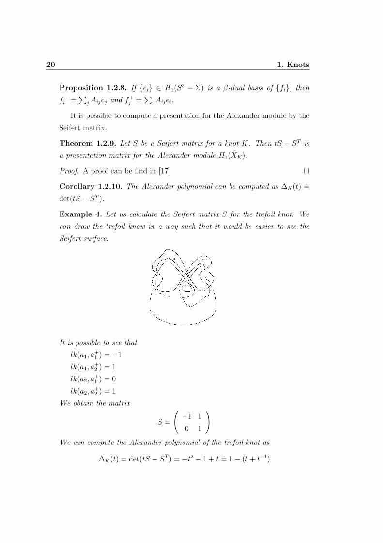
Example 4. Let us calculate the Seifert matrix S for the trefoil knot. We
can draw the trefoil know in a way such that it would be easier to see the
Seifert surface.
It is possible to see that
lk(a1, a+1 ) = −1
lk(a1, a+2 ) = 1
lk(a2, a+1 ) = 0
lk(a2, a+2 ) = 1
We obtain the matrix
S =
(−1 1
0 1
)We can compute the Alexander polynomial of the trefoil knot as
∆K(t) = det(tS − ST ) = −t2 − 1 + t.
= 1− (t+ t−1)
1.2 The Alexander-Conway polynomial 21
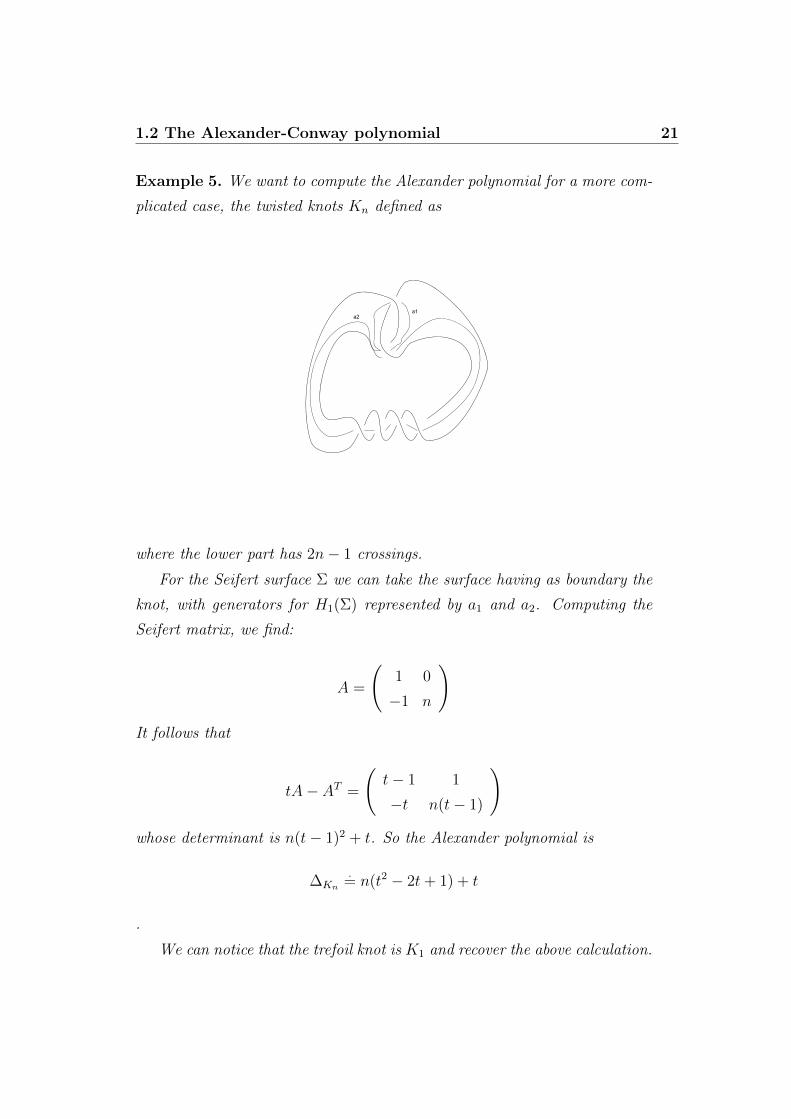
Example 5. We want to compute the Alexander polynomial for a more com-
plicated case, the twisted knots Kn defined as
a1a2
where the lower part has 2n− 1 crossings.
For the Seifert surface Σ we can take the surface having as boundary the
knot, with generators for H1(Σ) represented by a1 and a2. Computing the
Seifert matrix, we find:
A =
(1 0
−1 n
)It follows that
tA− AT =
(t− 1 1
−t n(t− 1)
)whose determinant is n(t− 1)2 + t. So the Alexander polynomial is
∆Kn
.= n(t2 − 2t+ 1) + t
.
We can notice that the trefoil knot is K1 and recover the above calculation.
22 1. Knots
Using this definition it is very easy to prove some results about the
Alexander polynomial.
Theorem 1.2.11. For any oriented link L, ∆L(t).
= ∆L(t−1). For any
oriented knot K, ∆K(1) = ±1.
Proof. The first statement is just an application of the standard theorems
on linear algebra.
∆L(t−1) = det(t−1A− AT ) = t−n det(A− tAt) .= det(tAt − A) = ∆L(t)
Now, let A be the Seifert matrix for K and Σ be the associated Seifert
surface. If Σ has genus g, H1(Σ) is 2g-dimensional and a basis is given
by fi. By theorem 1.2.9, ∆K(1) = ± det(A − AT ), where (A − AT )ij =
lk(f−i , fj) − lk(f+i , fj), which is the algebraic number of intersections of fi
and fj on Σ. We can see A− AT as made by g blocks(0 1
−1 0
)
in the diagonal and 0 elsewhere. So, computing the determinant, we have
proven the statement.
Corollary 1.2.12. For any knot K, ∆K(t).
= a0 +a1(t+ t−1)+a2(t2 + t−2)+
. . .+ an(tn + t−n), where ai are integers and a0 is odd.
Proof. If the degree of the Alexander polynomial ∆K(t) is odd, there is a
contradiction with theorem 1.2.11. By construction of the Seifert matrix, all
the ai must be integers. If we calculate ∆K(1) = a0 + 2a1 + . . . + 2an = ±1
we have that a0 ± 1 = 2(a0 + . . .+ an), so it has to be odd.
Remark 14. Usually, the signs for the coefficients ai are chosen such that
∆K(1) = 1.

1.2 The Alexander-Conway polynomial 23
Corollary 1.2.13. Let L be an oriented link. Let L be the reflection of L
and rL its reverse. Then ∆L(t) = ∆L(t) = ∆rL(t).
Proof. If S is the Seifert matrix for L, then −A is the Seifert matrix for L
and AT is the Seifert matrix for rL.
1.2.3 Fox differential calculus
Given a group G, we want to define the group ring Z[G]. Let ν : G→ Zbe such that ν(g) = 0 except for a finite number of elements of G. The
homomorphism ν has the following proprieties:
• (ν1 + ν2)(g) = ν1(g) + ν2(g),
• (ν1ν2)(g) =∑
h∈G(ν1(g)ν2(h−1g)).
Let us define the ’dual space’ G∗, consisting of elements g∗ such that
g∗(h) =
1 if g=h
0 otherwise
So, if g1, . . . , gk ∈ G and ni = ν(gi) we can set
ν = n1g∗1 + . . .+ nkg
∗k
In the following we will denote Z[G] as ZG.
Remark 15. ZG is a commutative ring if and only if G is an abelian group.
Remark 16. If Φ : G → A, A abelian ring, then there exists an extension
Φ : ZG→ A, Φ ring homomorphism.
Remark 17. If Φ : G → G′ is a group homomorphism, then Φ admits an
extension Φ : ZG→ ZG, Φ a ring homomorphism.
Let θ : G→ Z be the trivial morphism, θ(g) = 1 ∀g ∈ G. This morphism
can be extended to aug : ZG→ Z, aug(∑k
i=1 nigi) =∑k
i=1 ni.
24 1. Knots
Definition 18. A derivation D is an application D : ZG→ ZG such that
1. D(ν1 + ν2) = D(ν1) +D(ν2),
2. D(ν1ν2) = (Dν1)aug(ν2) + ν1D(ν2).
Remark 18. If g1, g2 ∈ G, D(g1g2) = D(g1) + g1D(g2).
Proposition 1.2.14. If D is a derivation then
• D(∑
i nigi) =∑
i niD(gi),
• D(n) = 0, ∀n ∈ Z,
• ∀g ∈ G, Dg−1 = −g−1Dg,
Proof. The first statement is a trivial consequence of linearity.
D(1) = D(1 · 1) = D(1) + 1 · D(1) = D(1) + D(1), then D(1) = 0. By
linearity, D(n) = 0 ∀n ∈ Z.
0 = D(1) = D(g−1g) = D(g−1) + g−1D(g), then D(g−1) = −g−1D(g).
Proposition 1.2.15. ∀n > 0 Dgn =∑n−1
i=0 gi and Dg−n = −
∑−1i=−n g
i.
Proof. It is easily seen by induction on n.
Theorem 1.2.16. Let F be the free group generated by n elements,
F =< x1, . . . , xn > .
For every generator xi of F there is an unique derivation Di = ∂∂xi
in ZFsuch that
∂xj∂xi
= δij
Proof. The proof, made by Fox, is included in his works [9], [10] and [11].
Corollary 1.2.17. Let h1(x), . . . , hn(x) be such that h1(x), . . . , hn(x) ∈ Z[F ].
It exists an unique derivation D in ZF such that Dxj = hj(x). For all
f(x) ∈ ZF , Df(x) =∑ ∂f
∂xjhj(x).
1.2 The Alexander-Conway polynomial 25
Theorem 1.2.18. β : f(x) 7→ f(x)− f(1) is a derivation.
f(x)− f(1) =∑
1
∂f
∂xi(xi − 1)
Theorem 1.2.18 is called the fundamental theorem of Fox calculus.
LetG be a group and P be a finite representation, P =< x1, . . . , xn| r1, . . . , rk >.
Let Fn =< x1, . . . , xn > be the free group generated by x1, . . . , xn, H the
normal subgroup generated by r1, . . . , rk. Then Fn/H ' G, g 7→ g. This
function can be extended to ZFn → ZG, a 7→ a.
Definition 19. The Fox matrix associated to the group G with presentation
P is the k × n matrix with coefficients in ZG
F (G,P ) = (∂ri∂j
), 1 ≤ i ≤ k, 1 ≤ j ≤ n
We now show that the Fox matrix is well defined, i.e. it is independent of
the choice of the presentation P . To do that, we will use the so-called Tietze
presentation.
Definition 20. Let A and A′ be two matrices with coefficients in the same
ring R. A and A′ are T -equivalent if it is possible to obtain one from the
other by a sequence of following operations or of their inverses:
1. permutations of rows and columns
2. adding to a row (respectively column) a linear combination of other
rows (respectively columns)
3. changing the matrix A by the matrix(1 ∗0 A
)
Theorem 1.2.19. Let P =< x1, . . . , xn| r1, . . . , rk > be a presentation of
the group G. If P ′ is another presentation, then it is possible to obtain P ′
from P by a finite number of Tietze transformations and their inverses:
26 1. Knots
1. adding a new relation r such that r ∈ H,
2. adding a new generator x and a relation xw, where w is a word in
x1, . . . , xn.
Proof. A proof can be found in [18].
Theorem 1.2.20. Let P and P ′ be two finite representations of the same
group G. Then the Fox matrices F (G,P ) and F (G,Q) are T -equivalent.
Proof. A permutation of rows and columns corresponds to a permutation of
generators and relations.
Let now P =< x1 . . . , xn| r1, . . . , rk > be a presentation of G. We add a
relation s ∈ H. So,
s =m∏i=1
uirεii u−1i
where ui is a word in xi, εi = ±1, ri ∈ H. We can split it in three different
cases and get the propriety for linearity.
Case s = r1r2. In ZFn, ∂s∂xi
= ∂r1∂xi
+r1∂r2∂xi
. So in ZG we get ∂s∂xi
= ∂r1∂xi
+ ∂r2∂xi
,
that is adding a row.
Case s = uru−1, r ∈ H, u word in x1, . . . , xn.
∂s
∂xi=
∂u
∂xi+ u(
∂r
∂xi− ru−1 ∂u
∂xi) = u
∂r
∂xi+ (1− uru−1)
∂u
∂xi
So ∂s∂xi
= u ∂r∂xi
+ (1− s) ∂u∂xi
. In ZG we have
∂s
∂xi= u
∂r
∂xi
which is multiplying a row on the left.
Case s = r−1, r ∈ H.∂s
∂xi= −r−1 ∂r
∂xi
So ∂s∂xi
= − ∂r∂xi
, multiplying a row for −1.
1.2 The Alexander-Conway polynomial 27
Now, if P ′ =< x1, . . . , xn, x| xw, r1, . . . , rk >, we get the matrix
F (G,P ′) =
(1 ∂w/∂xi
0 F (G,P )
)
Definition 21. Let R be a commutative ring, α : ZG→ R a homomorphism,
F (G,P, α) = α(∂ri∂xj
)
We call E(G,P, α) the ideal generated by the minors of order n− 1.
Lemma 1.2.21. E(G,P, α) is independent of the presentation P .
Proof. If P ′ is another presentation of the group G, then F (G,P, α) and
F (G,Q, α) are T -equivalent.
Permuting rows and columns and adding linear combination of rows
(columns) to another row (column) leaves unchanged the minors. We have
just to check the case F is changed in F ′ =
(1 ∗0 F
), where ∗ is a n − 1
array. F has n columns, while F ′ has n+ 1-columns.
Every minor of F of order n− 1 lies in a minor of F ′ of order n, so that
E ⊂ E ′.
Every minor of order n of F ′ is a linear combination of minors of F of
order n− 1, so E ′ ⊂ E.
1.2.4 Fox differential calculus for knots groups
Let us now focus on knots groups. LetK ⊂ S3 be a knot, ΓK = π1(S3−K)
the knot group. We take P =< x1, . . . , xn| r1, . . . , rn−1 > as the Wirtinger
presentation of ΓK . Let α : ΓK → Z be such that α(xi) = t, ∀i, 1 ≤ i ≤ n.
We have Z[Z] = Z[t, t−1], the ring of Laurent polynomials. We can extend α
to α : Z[ΓK ]→ Z[t, t−1], a ring homomorphism. In the following we will call,
with a little abuse of notation, α = α.
28 1. Knots
Definition 22. The Alexander ideal of a knot K is E(K) = E(ΓK , α).
Theorem 1.2.22. E(K) is a principal ideal.
Proof. The fundamental theorem of Fox calculus implies that if
x ∈ Fn =< x1, . . . , xn >,
then
x− 1 =n∑j=1
∂x
∂xj(xj − 1).
Also,
ri − 1 =n∑j=1
∂ri∂xj
(xj − 1),∀ i = 1, . . . , n− 1.
So,∑n
j=1∂ri∂xj
(xj − 1) = ri − 1 = 0 and∑n
j=1 α( ∂ri∂xj
) = 0 in Z[t, t−1].
We have then that if the matrix is F = (aij),∑n
j=1 aij = 0, ∀ i : 1 ≤ i ≤n−1. If c1, . . . , cn are the columns of F (ΓK , F, α) = (aij), then c1 + . . .+cn =
0.
By definition, the Alexander ideal is generated by det(A1), . . . , det(An).
We have
det(A1) = det(c2, . . . , cn) = det(c2 + . . .+ cn, c3, . . . , cn) =
det(−c1, c3, . . . , cn) = − det(A1).
So, with similar considerations, we get det(Ai) = det(±Aj) and E(K) is
then generated by only one of the det(Ai).
Theorem 1.2.23. A generator of the ideal E(K) is the Alexander polynomial
∆K(t).
Proof. A proof can be found in [8] or [17].
1.2 The Alexander-Conway polynomial 29
Remark 19. All the considerations above can be done if we took the Wirtinger
presentation. If we have another presentation, it is not true in general that
the ideal E(K) is generated by a minor Ai.
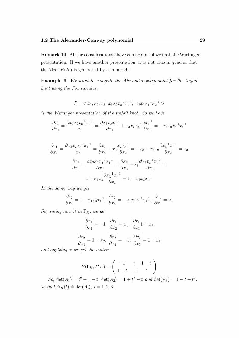
Example 6. We want to compute the Alexander polynomial for the trefoil
knot using the Fox calculus.
P =< x1, x2, x3| x3x2x−13 x−1
1 , x1x3x−11 x−1
2 >
is the Wirtinger presentation of the trefoil knot. So we have
∂r1
∂x1
=∂x3x2x
−13 x−1
1
x1
=∂x3x2x
−13
∂x1
+ x3x2x−13
∂x−11
∂x1
= −x3x2x−13 x−1
1
∂r1
∂x2
=∂x3x2x
−13 x−1
1
x2
=∂x3
∂x2
+ x3x2x
−13
∂x2
= −x3 + x3x2∂x−1
3 x−11
∂x2
= x3
∂r1
∂x3
=∂x3x2x
−13 x−1
1
∂x3
=∂x3
∂x3
+ x3∂x2x
−13 x−1
1
∂x3
=
1 + x3x2∂x−1
3 x−11
∂x3
= 1− x3x2x−13
In the same way we get
∂r2
∂x1
= 1− x1x3x−11 ,
∂r2
∂x2
= −x1x3x−11 x−1
2 ,∂r1
∂x3
= x1
So, seeing now it in ΓK, we get
∂r1
∂x1
= −1,∂r1
∂x2
= x3,∂r1
∂x1
1− x1
∂r2
∂x1
= 1− x2,∂r2
∂x2
= −1,∂r2
∂x3
= 1− x1
and applying α we get the matrix
F (ΓK , P, α) =
(−1 t 1− t
1− t −1 t
)So, det(A1) = t2 + 1− t, det(A2) = 1 + t2 − t and det(A3) = 1 − t + t2,
so that ∆K(t).
= det(Ai), i = 1, 2, 3.
30 1. Knots
Let us now see what happens if we take a group representation that is not
Wirtinger’s. We take as presentation
Q =< a, b| a2b−3 > .
We had calculated it by passing by the presentation < x, y|xyx = yxy >
and taking xyx = a, xy = b. So, α(x) = t3, α(y) = t2. We have
∂r
∂a= (1 + a),
∂r
∂b= a2(−b−1 − b−2 − b−3)
So we get
F (ΓK , Q, α) = (1 + t3 − 1− t2 − t4).
By factorisation
1 + t3 = (1 + t)(1− t+ t2)
1 + t2 + t4 = (1 + t+ t2)(1− t+ t2)
and E(K) = ∆K(t) = 1− t+ t2.
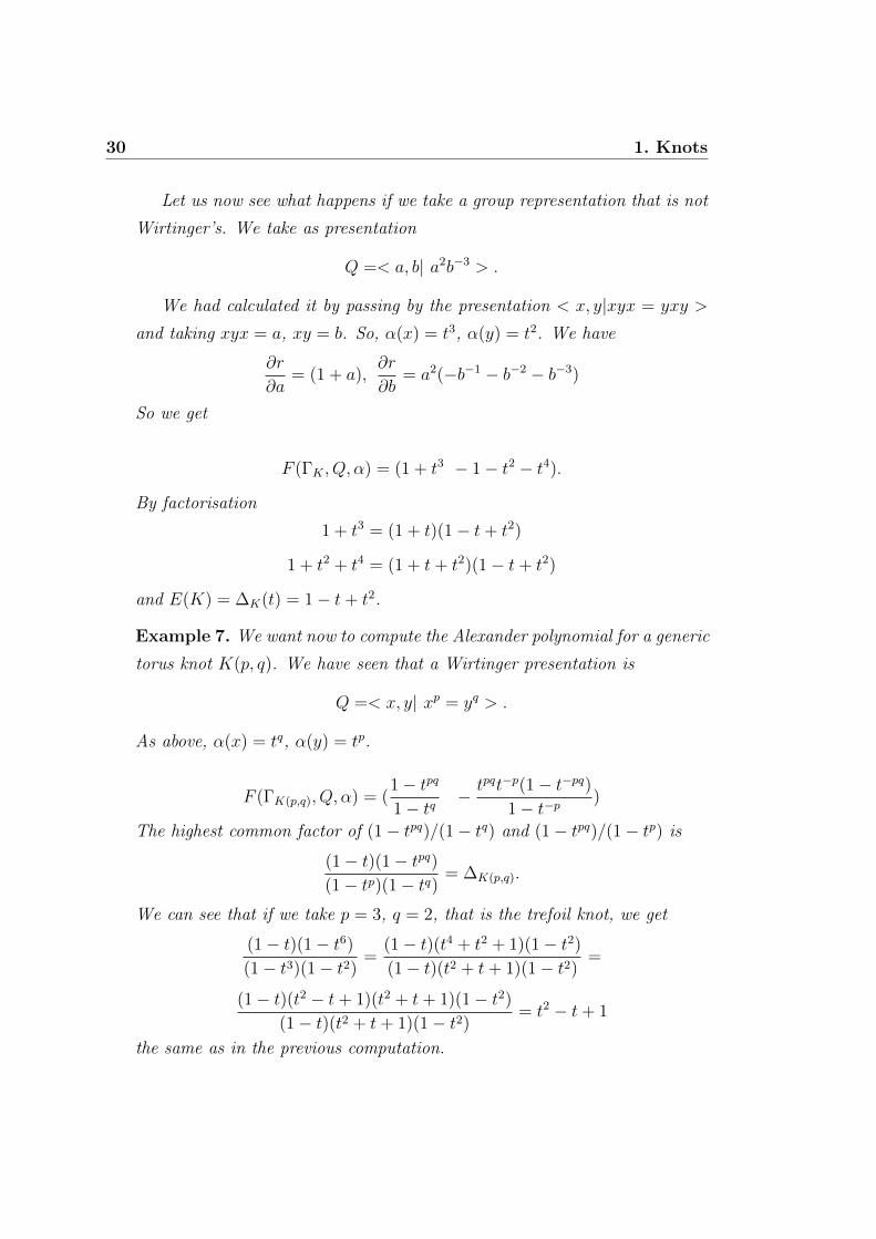
Example 7. We want now to compute the Alexander polynomial for a generic
torus knot K(p, q). We have seen that a Wirtinger presentation is
Q =< x, y| xp = yq > .
As above, α(x) = tq, α(y) = tp.
F (ΓK(p,q), Q, α) = (1− tpq
1− tq− tpqt−p(1− t−pq)
1− t−p)
The highest common factor of (1− tpq)/(1− tq) and (1− tpq)/(1− tp) is
(1− t)(1− tpq)(1− tp)(1− tq)
= ∆K(p,q).
We can see that if we take p = 3, q = 2, that is the trefoil knot, we get
(1− t)(1− t6)
(1− t3)(1− t2)=
(1− t)(t4 + t2 + 1)(1− t2)
(1− t)(t2 + t+ 1)(1− t2)=
(1− t)(t2 − t+ 1)(t2 + t+ 1)(1− t2)
(1− t)(t2 + t+ 1)(1− t2)= t2 − t+ 1
the same as in the previous computation.
1.2 The Alexander-Conway polynomial 31
1.2.5 The Alexander-Conway polynomial
We will now show how it is possible to normalise the Alexander polyno-
mial such that it has no more the ambiguity concerning multiplication by
units of Z[t±]. We start by some considerations about Seifert matrices.
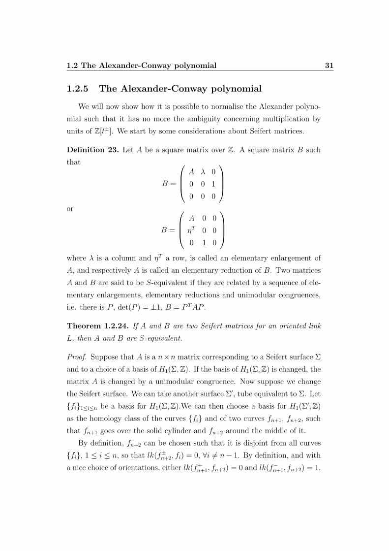
Definition 23. Let A be a square matrix over Z. A square matrix B such
that
B =
A λ 0
0 0 1
0 0 0
or
B =
A 0 0
ηT 0 0
0 1 0
where λ is a column and ηT a row, is called an elementary enlargement of
A, and respectively A is called an elementary reduction of B. Two matrices
A and B are said to be S-equivalent if they are related by a sequence of ele-
mentary enlargements, elementary reductions and unimodular congruences,
i.e. there is P , det(P ) = ±1, B = P TAP .
Theorem 1.2.24. If A and B are two Seifert matrices for an oriented link
L, then A and B are S-equivalent.
Proof. Suppose that A is a n×n matrix corresponding to a Seifert surface Σ
and to a choice of a basis of H1(Σ,Z). If the basis of H1(Σ,Z) is changed, the
matrix A is changed by a unimodular congruence. Now suppose we change
the Seifert surface. We can take another surface Σ′, tube equivalent to Σ. Let
fi1≤i≤n be a basis for H1(Σ,Z).We can then choose a basis for H1(Σ′,Z)
as the homology class of the curves fi and of two curves fn+1, fn+2, such
that fn+1 goes over the solid cylinder and fn+2 around the middle of it.
By definition, fn+2 can be chosen such that it is disjoint from all curves
fi, 1 ≤ i ≤ n, so that lk(f±n+2, fi) = 0, ∀i 6= n− 1. By definition, and with
a nice choice of orientations, either lk(f+n+1, fn+2) = 0 and lk(f−n+1, fn+2) = 1,
32 1. Knots
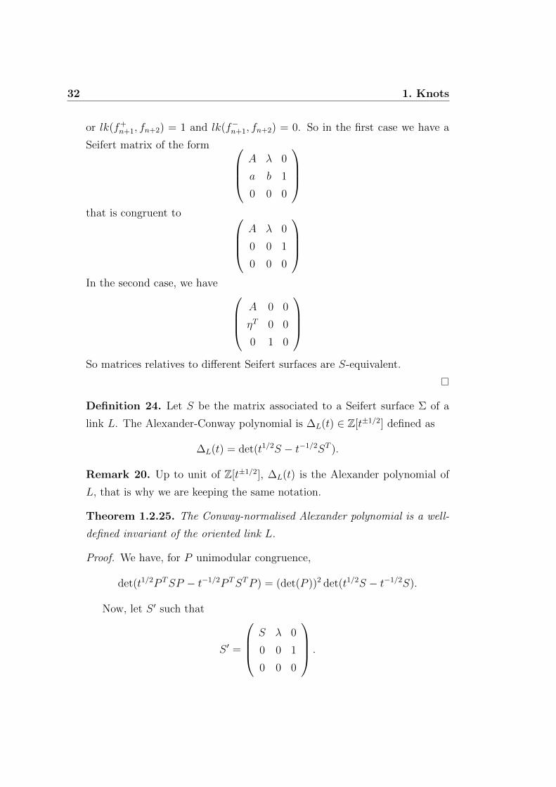
or lk(f+n+1, fn+2) = 1 and lk(f−n+1, fn+2) = 0. So in the first case we have a
Seifert matrix of the form A λ 0
a b 1
0 0 0
that is congruent to
A λ 0
0 0 1
0 0 0
In the second case, we have
A 0 0
ηT 0 0
0 1 0
So matrices relatives to different Seifert surfaces are S-equivalent.
Definition 24. Let S be the matrix associated to a Seifert surface Σ of a
link L. The Alexander-Conway polynomial is ∆L(t) ∈ Z[t±1/2] defined as
∆L(t) = det(t1/2S − t−1/2ST ).
Remark 20. Up to unit of Z[t±1/2], ∆L(t) is the Alexander polynomial of
L, that is why we are keeping the same notation.
Theorem 1.2.25. The Conway-normalised Alexander polynomial is a well-
defined invariant of the oriented link L.
Proof. We have, for P unimodular congruence,
det(t1/2P TSP − t−1/2P TSTP ) = (det(P ))2 det(t1/2S − t−1/2S).
Now, let S ′ such that
S ′ =
S λ 0
0 0 1
0 0 0
.
1.2 The Alexander-Conway polynomial 33
So,
(t1/2S ′ − t−1/2S ′T ) =
t1/2S − t1/2St t1/2λ 0
−t−1/2λT 0 t1/2
0 t−1/2 0
which has the same determinant as t1/2S − t−1/2ST . In the same way, the
other type of elementary enlargement of S has no effect on the determinant.
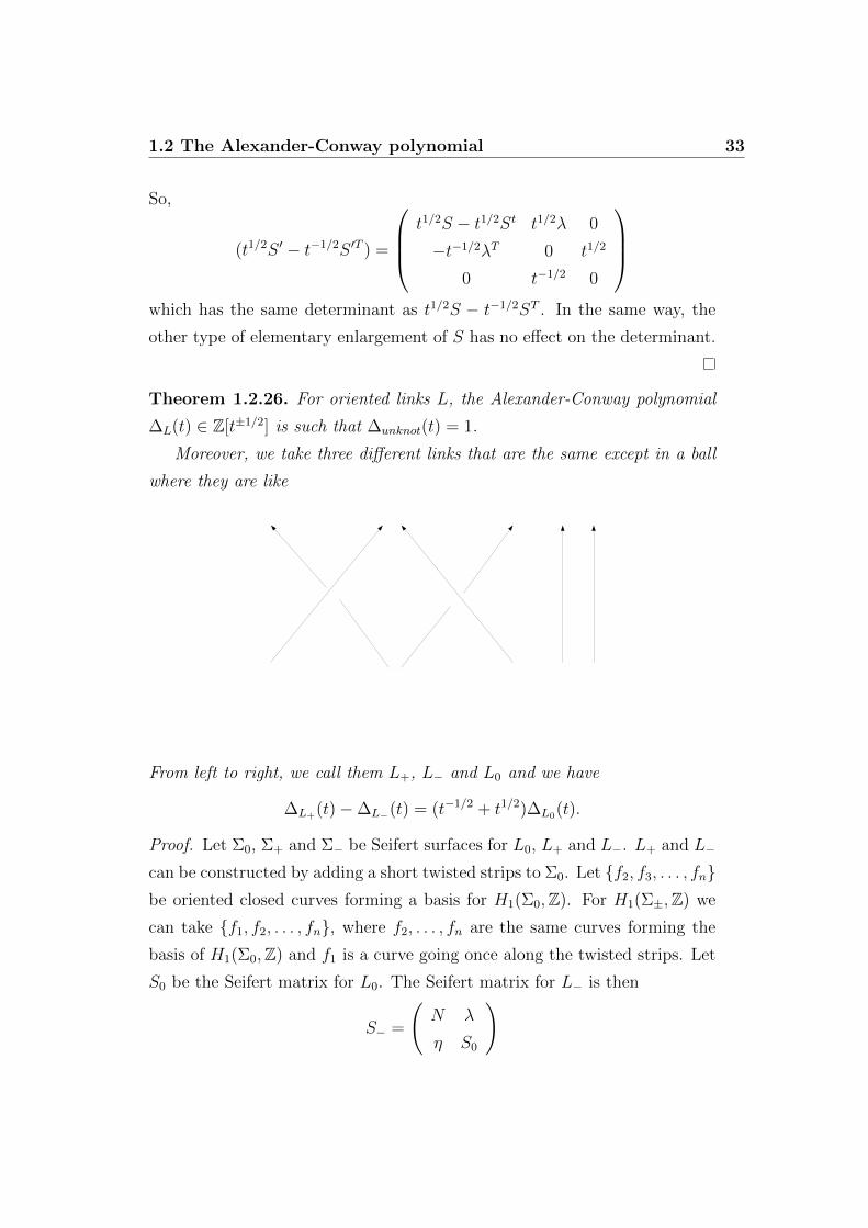
Theorem 1.2.26. For oriented links L, the Alexander-Conway polynomial
∆L(t) ∈ Z[t±1/2] is such that ∆unknot(t) = 1.
Moreover, we take three different links that are the same except in a ball
where they are like
From left to right, we call them L+, L− and L0 and we have
∆L+(t)−∆L−(t) = (t−1/2 + t1/2)∆L0(t).
Proof. Let Σ0, Σ+ and Σ− be Seifert surfaces for L0, L+ and L−. L+ and L−
can be constructed by adding a short twisted strips to Σ0. Let f2, f3, . . . , fnbe oriented closed curves forming a basis for H1(Σ0,Z). For H1(Σ±,Z) we
can take f1, f2, . . . , fn, where f2, . . . , fn are the same curves forming the
basis of H1(Σ0,Z) and f1 is a curve going once along the twisted strips. Let
S0 be the Seifert matrix for L0. The Seifert matrix for L− is then
S− =
(N λ
η S0
)

34 1. Knots
whereas the Seifert matrix for L+ is
S+ =
(N − 1 λ
η S0
)
Now, computing det(t1/2S+−t−1/2ST+)−det(t1/2S−−t1/2ST−) gives exactly
det(t1/2S0 − t−1/2S0).
1.3 The Jones polynomial
1.3.1 Definition by Kaufmann brackets
Definition 25. The Kauffman bracket is a function from unoriented link
diagrams to Laurent polynomials with integer coefficients in an indeterminate
A, <>: D → Z[A±], such that
1. < unknot >= 1,
2. < D q unknot >= (−A−2 − A2) < D >,
3. < C+ >= A < C1 > +A−1 < C2 >.
where C+, C1 and C2 are such that
The third propriety means that the three link diagrams are the same,
except near a point where they differ in the way indicated in the picture.
Remark 21. The bracket polynomial of a diagram with n crossings can be
calculated by expressing it as a sum of 2n diagrams with no crossings, then
applying proprieties 1 and 2.
1.3 The Jones polynomial 35
We want now to see what happens changing the diagram D by a Reide-
meister move.
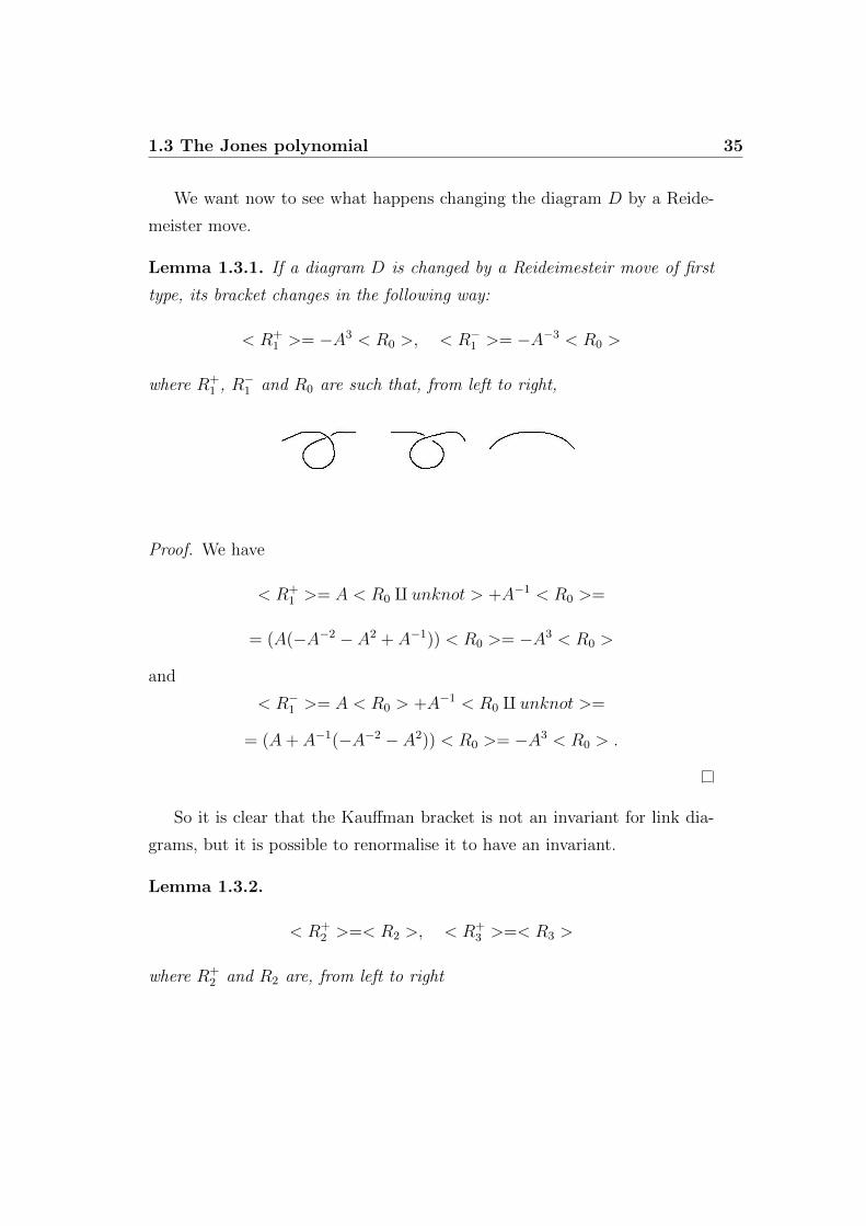
Lemma 1.3.1. If a diagram D is changed by a Reideimesteir move of first
type, its bracket changes in the following way:
< R+1 >= −A3 < R0 >, < R−1 >= −A−3 < R0 >
where R+1 , R−1 and R0 are such that, from left to right,
Proof. We have
< R+1 >= A < R0 q unknot > +A−1 < R0 >=
= (A(−A−2 − A2 + A−1)) < R0 >= −A3 < R0 >
and
< R−1 >= A < R0 > +A−1 < R0 q unknot >=
= (A+ A−1(−A−2 − A2)) < R0 >= −A3 < R0 > .
So it is clear that the Kauffman bracket is not an invariant for link dia-
grams, but it is possible to renormalise it to have an invariant.
Lemma 1.3.2.
< R+2 >=< R2 >, < R+
3 >=< R3 >
where R+2 and R2 are, from left to right
36 1. Knots
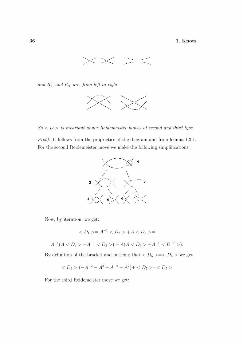
and R+3 and R−3 are, from left to right
So < D > is invariant under Reidemeister moves of second and third type.
Proof. It follows from the proprieties of the diagram and from lemma 1.3.1.
For the second Reidemeister move we make the following simplifications:
Now, by iteration, we get:
< D1 >= A−1 < D2 > +A < D3 >=
A−1(A < D4 > +A−1 < D5 >) + A(A < D6 > +A−1 < D−7 >).
By definition of the bracket and noticing that < D5 >=< D6 > we get
< D5 > (−A−2 − A2 + A−2 + A2)+ < D7 >=< D7 >
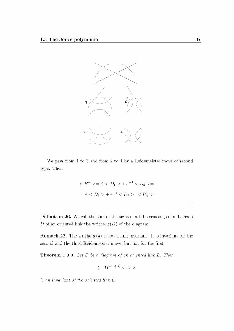
For the third Reidemeister move we get:
1.3 The Jones polynomial 37
1 2
3 4
We pass from 1 to 3 and from 2 to 4 by a Reidemeister move of second
type. Then
< R+3 >= A < D1 > +A−1 < D2 >=
= A < D3 > +A−1 < D4 >=< R−3 >
Definition 26. We call the sum of the signs of all the crossings of a diagram
D of an oriented link the writhe w(D) of the diagram.
Remark 22. The writhe w(d) is not a link invariant. It is invariant for the
second and the third Reidemeister move, but not for the first.
Theorem 1.3.3. Let D be a diagram of an oriented link L. Then
(−A)−3w(D) < D >
is an invariant of the oriented link L.
38 1. Knots
Proof. By lemma 1.3.2 and remark 22 this expression is invariant for second
and third Reidemeister move. By the computation done for the first Reide-
meister move we have that is also unchanged for first Reidemeister move.
Definition 27. Given a diagram D of a link L, we define the Jones polyno-
mial V (L) as the Laurent polynomial in t1/2 with integer coefficients, defined
by
V (L) = ((−A)−3w(D) < D >)t1/2=A−2 .
For theorem 1.3.3, V (L) is well defined.
1.3.2 Definition by skein relations
As for the Alexander-Conway polynomial, we now show that it is possible
to define it using skein relations.
Proposition 1.3.4. The Jones polynomial is a function
V : oriented links in S3 → Z[t±1/2]
such that V (unknot) = 1 and that
t−1V (L+)− tV (L−) + (t−1/2 − t1/2)V (L0) = 0
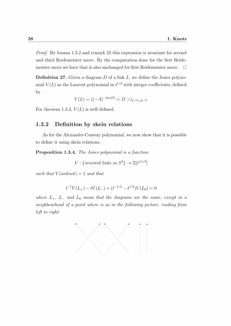
where L+, L− and L0 mean that the diagrams are the same, except in a
neighbourhood of a point where is as in the following picture, reading from
left to right:
1.3 The Jones polynomial 39
Proof. Let us take into consideration the diagrams C1 = L0, C2 of the defi-
nition of the Kauffman bracket. We have
< L+ >= A < C1 > +A−1 < C2 >, < L− >= A−1 < C1 > +A < C2 >
so that A < L+ > −A−1 < L− >= (A2 − A−2) < L0 >.
By definition, w(L+)− 1 = w(L0)) = w(L−) + 1 and so
−A4V (L+) + A−4V (L−) = (A2 − A−2)V (L0).
Up to the substitution t1/2 = A−2 we have the thesis.
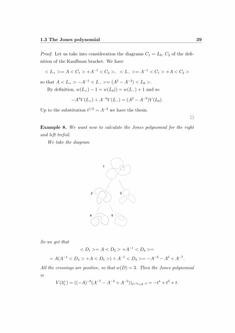
Example 8. We want now to calculate the Jones polynomial for the right
and left trefoil.
We take the diagram
1
2 3
4 5
So we get that
< D1 >= A < D2 > +A−1 < D3 >=
= A(A−1 < D4 > +A < D5 >) + A−1 < D3 >= −A−3 − A5 + A−7.
All the crossings are positive, so that w(D) = 3. Then the Jones polynomial
is
V (3+1 ) = ((−A)−9(A−7 − A−3 + A−5))t1/2=A−2 = −t4 + t3 + t.
40 1. Knots
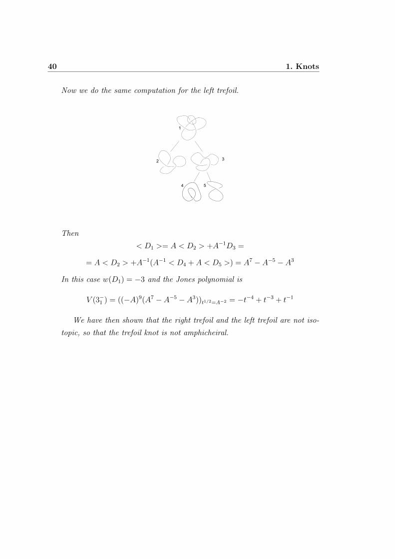
Now we do the same computation for the left trefoil.
1
2 3
4 5
Then
< D1 >= A < D2 > +A−1D3 =
= A < D2 > +A−1(A−1 < D4 + A < D5 >) = A7 − A−5 − A3
In this case w(D1) = −3 and the Jones polynomial is
V (3−1 ) = ((−A)9(A7 − A−5 − A3))t1/2=A−2 = −t−4 + t−3 + t−1
We have then shown that the right trefoil and the left trefoil are not iso-
topic, so that the trefoil knot is not amphicheiral.
Chapter 2
Braid groups
2.1 Some equivalent definitions
2.1.1 Configuration spaces
Definition 28. Let ∆ ⊂ Cn, n ∈ N be
∆ = ∪ni,j=1zi = zj, i 6= j.
Let C and Confn be such that C = Cn−∆ and Confn(C) = (Cn−∆)/Sn,
where Sn is the group of permutation on n elements.
Remark 23. The space C, associated to the map C → Confn(C), is a
covering space of Confn(C) and the associated group is Sn.
Remark 24. Up to homeomorphism, it is possible to consider just points in
the interior of D2 ⊂ C.
Let ∗ be the point on the real line, ∗ = 2k−1−nn
, 1 ≤ k ≤ n.
Definition 29. We call n-pure braid group the group
Pn = π1(C, ∗).
We call n-braid group the group
Bn = π1(Confn(C), ∗).
41
42 2. Braid groups
2.1.2 Diagrams
Let I be the closed interval [0, 1] ⊂ R. A topological interval is a topo-
logical space homeomorphic to I.
Definition 30. A geometric braid on n strings, n ≥ 1, is a set b ⊂ C × Iformed by n disjoints topological intervals, the strings of b, such that the
projection C× I → I maps each string homeomorphically onto I and
b ∩ (C× 0) = ∗ × 0
b ∩ (C× 1) = ∗ × 1
where ∗ is the set of points defined above. We can label the n points by
P = (p1, . . . , pn) = 1, . . . , n.
Remark 25. Every string of b meets each C × t, t ∈ I, in exactly one
point and connects a point in P × 0 to a point in P × 1.We can associate to each string b a permutation π ∈ Sn such that
b(Pi, 1) = π(i).
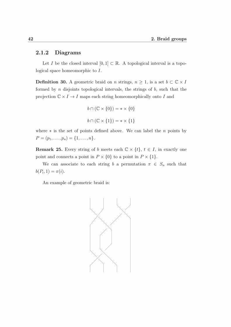
An example of geometric braid is:
2.1 Some equivalent definitions 43
The underlying permutations is (3 4).
We want now to define a class of isotopy for braids, as it is for knots.
Definition 31. Let b and b′ be two geometric braids. They are said to be
isotopic if there is a continuous map F : b× I → C× I such that
• for each s ∈ I Fs : b → C × I is an embedding, whose image is a
geometric braid on n strings,
• F0 = idb : b→ b,
• F1(b) = b′.
Remark 26. If b and b′ are isotopic, then the underlying permutations πb
and πb′ must be the same.
Proposition 2.1.1. The relation of isotopy is an equivalence relation. We
call the equivalence classes braids on n strings.
We want now to introduce a canonical operation between two braids. We
will see that the set of geometric braids with this operation is actually a
group.
Definition 32. Let b1 and b2 be two n-strands geometric braids. We define
b = b1b2 as the set of points z, t ∈ C × I such that z, 2t ∈ b1, for
0 ≤ t ≤ 1/2 and z, 2t− 1 ∈ b2 for 1/2 ≤ t ≤ 1. b is still a geometric braid
with n strands.
Remark 27. If b1 is isotopic to b′1 and b2 is isotopic to b′2, then b1b2 is isotopic
to b′1b′2.
As we have done for knots, we would like to represent geometric braids
on the plane. In the following we will identify C with R2.
Definition 33. A braid diagram on n strands is a set D ⊂ R× I, union of
n topological intervals, such that:
• the projection R× I → I maps each strand homeomorphically onto I,

44 2. Braid groups
• every point of ∗ × 0, 1 is the endpoint of a unique strand,
• every point of R× I belongs to at most two strands. At each crossing
these strands meet transversely, with one undergoing and the other
overgoing.
Remark 28. By compactness of the strands, the number of crossing of a
diagram D is finite.
Proposition 2.1.2. Every geometric braid can be represented by a braid
diagram.
Every braid diagram represents a geometric braid, up to isotopy.
Definition 34. Two braid diagrams D and D′ on n strands are said to be
isotopic if there is a map F : D × I → R× I such that
• F (D × s) is a braid diagram on n strands ∀s ∈ I,
• D0 = D,
• D1 = D′.
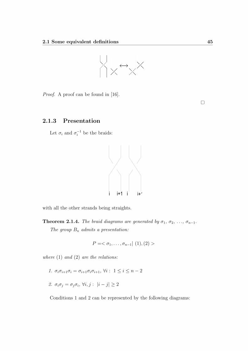
Theorem 2.1.3. Two braid diagrams D and D′ define the same geometric
braid if and only if it is possible to get one from the other by a sequence of
diagram moves and their inverses as following:
2.1 Some equivalent definitions 45
Proof. A proof can be found in [16].
2.1.3 Presentation
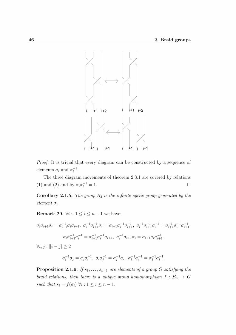
Let σi and σ−1i be the braids:
i+1ii+1i
with all the other strands being straights.
Theorem 2.1.4. The braid diagrams are generated by σ1, σ2, . . ., σn−1.
The group Bn admits a presentation:
P =< σ1, . . . , σn−1| (1), (2) >
where (1) and (2) are the relations:
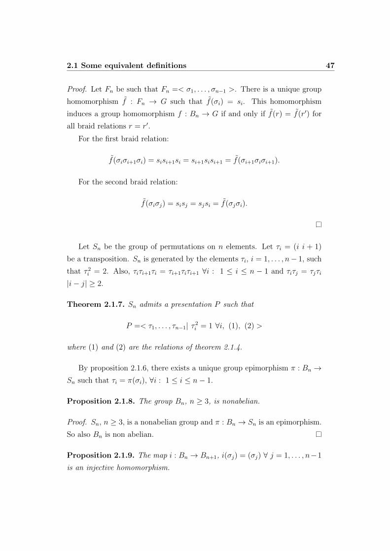
1. σiσi+1σi = σi+1σiσi+1, ∀i : 1 ≤ i ≤ n− 2
2. σiσj = σjσi, ∀i, j : |i− j| ≥ 2
Conditions 1 and 2 can be represented by the following diagrams:
46 2. Braid groups
i i+1 i+2 i i+1 i+2
i i+1 i+1ij jj+1 j+1
Proof. It is trivial that every diagram can be constructed by a sequence of
elements σi and σ−1i .
The three diagram movements of theorem 2.3.1 are covered by relations
(1) and (2) and by σiσ−1i = 1.
Corollary 2.1.5. The group B2 is the infinite cyclic group generated by the
element σ1.
Remark 29. ∀i : 1 ≤ i ≤ n− 1 we have:
σiσi+1σi = σ−1i+1σiσi+1, σ
−1i σ−1
i+1σi = σi+1σ−1i σ−1
i+1, σ−1i σ−1
i+1σ−1i = σ−1
i+1σ−1i σ−1
i+1,
σiσ−1i+1σ
−1i = σ−1
i+1σ−1i σi+1, σ
−1i σi+1σi = σi+1σiσ
−1i+1.
∀i, j : ‖i− j| ≥ 2
σ−1i σj = σjσ
−1i , σiσ
−1j = σ−1
j σi, σ−1i σ−1
j = σ−1j σ−1
i .
Proposition 2.1.6. If s1, . . . , sn−1 are elements of a group G satisfying the
braid relations, then there is a unique group homomorphism f : Bn → G
such that si = f(σi) ∀i : 1 ≤ i ≤ n− 1.
2.1 Some equivalent definitions 47
Proof. Let Fn be such that Fn =< σ1, . . . , σn−1 >. There is a unique group
homomorphism f : Fn → G such that f(σi) = si. This homomorphism
induces a group homomorphism f : Bn → G if and only if f(r) = f(r′) for
all braid relations r = r′.
For the first braid relation:
f(σiσi+1σi) = sisi+1si = si+1sisi+1 = f(σi+1σiσi+1).
For the second braid relation:
f(σiσj) = sisj = sjsi = f(σjσi).
Let Sn be the group of permutations on n elements. Let τi = (i i + 1)
be a transposition. Sn is generated by the elements τi, i = 1, . . . , n− 1, such
that τ 2i = 2. Also, τiτi+1τi = τi+1τiτi+1 ∀i : 1 ≤ i ≤ n − 1 and τiτj = τjτi
|i− j| ≥ 2.
Theorem 2.1.7. Sn admits a presentation P such that
P =< τ1, . . . , τn−1| τ 2i = 1 ∀i, (1), (2) >
where (1) and (2) are the relations of theorem 2.1.4.
By proposition 2.1.6, there exists a unique group epimorphism π : Bn →Sn such that τi = π(σi), ∀i : 1 ≤ i ≤ n− 1.
Proposition 2.1.8. The group Bn, n ≥ 3, is nonabelian.
Proof. Sn, n ≥ 3, is a nonabelian group and π : Bn → Sn is an epimorphism.
So also Bn is non abelian.
Proposition 2.1.9. The map i : Bn → Bn+1, i(σj) = (σj) ∀ j = 1, . . . , n−1
is an injective homomorphism.
48 2. Braid groups
We can see this map on geometric braids as the map sending every braid
β ∈ Bn in itself, with an additional straight strand on the far right. We have
then a sequence of inclusions B1 ⊂ B2 ⊂ B2 ⊂ . . ..
Composing i with the projection π : Bn+1 → Sn+1 it is the same than
composing π : Bn → Sn with the inclusion Sn → Sn+1. So there is a
commutative diagram
Bn −→ Sn
↓ ↓Bn+1 −→ Sn+1
Example 9. By definition, B3 =< σ1, σ2| σ1σ2σ1 = σ2σ1σ2 >.
This is exactly the knot group of the trefoil knot, as we have computed
in the first chapter. We can represent it also as < a, b| a2 = b3 >. We can
notice that, with that presentation, the element a2 lies in the center of B3.
Proposition 2.1.10. The group Bn admits a presentation with two genera-
tors.
Proof. Let α and β be such that α = σ1, β = σ1σ2, . . . , σn−1,
For 1 ≤ i ≤ n− 2 we have βσi = σi+1β.
(σ1σ2 . . . σn−1)σi = σ1σ2 . . . σi−1σiσi+1σiσi+2 . . . σn−1 =
σ1σ2 . . . σi−1σi+1σiσi+1 . . . σn−1 = σi+1(σ1σ2 . . . σn−1).
So it is easy to see that σi = βi−1αβ1−i and that α, β generate all Bn.
2.1.4 Mapping class groups
In the following Pn represents a set of n points on the real line of C (or
equivalently on the line R× 0 ⊂ R2).
Definition 35. Let Diff(D2, Pn, S1) be the set of diffeomorphisms f : D2 →
D2 such that f(Pn) = Pn and f |S1 = IdS1 , also called self diffeomorphisms.
Let Diff0(D2, Pn, S1) be the set of the self diffeomorphisms f : D2 → D2
2.1 Some equivalent definitions 49
such that every f is isotopic to IdD2 , i.e. there is a continuous family ft(x)
of self diffeomorphisms such that f0(x) = f(x) and f1(x) = x.
Proposition 2.1.11. Diff0(D2, Pn, S1) is a normal subgroup of Diff(D2, Pn, S
1).
Proof. It is easy to see that Diff0(D2, Pn, S1) is a subgroup.
If f ∈ Diff0(D2, Pn, S1), g ∈ Diff(D2, Pn, S
1) then g−1fg ' g−1Idg 'gg−1 ' IdD2 .
Definition 36. Let Dn2 be D2 with a choice of a set of n points Pn. We
define M(Dn2 ) as
M(Dn2 ) =
Diff(D2, Pn, S1)
Diff0(D2, Pn, S1).
Theorem 2.1.12. M(D02) = M(D2) is trivial.
Proof. We use the Alexander trick. Let f be such that f ∈ Diff(D2, S1).
Let us take
h(s, reiθ) =
f( r
1−seiθ), r ≤ 1− s
reiθ, r ≥ 1− s
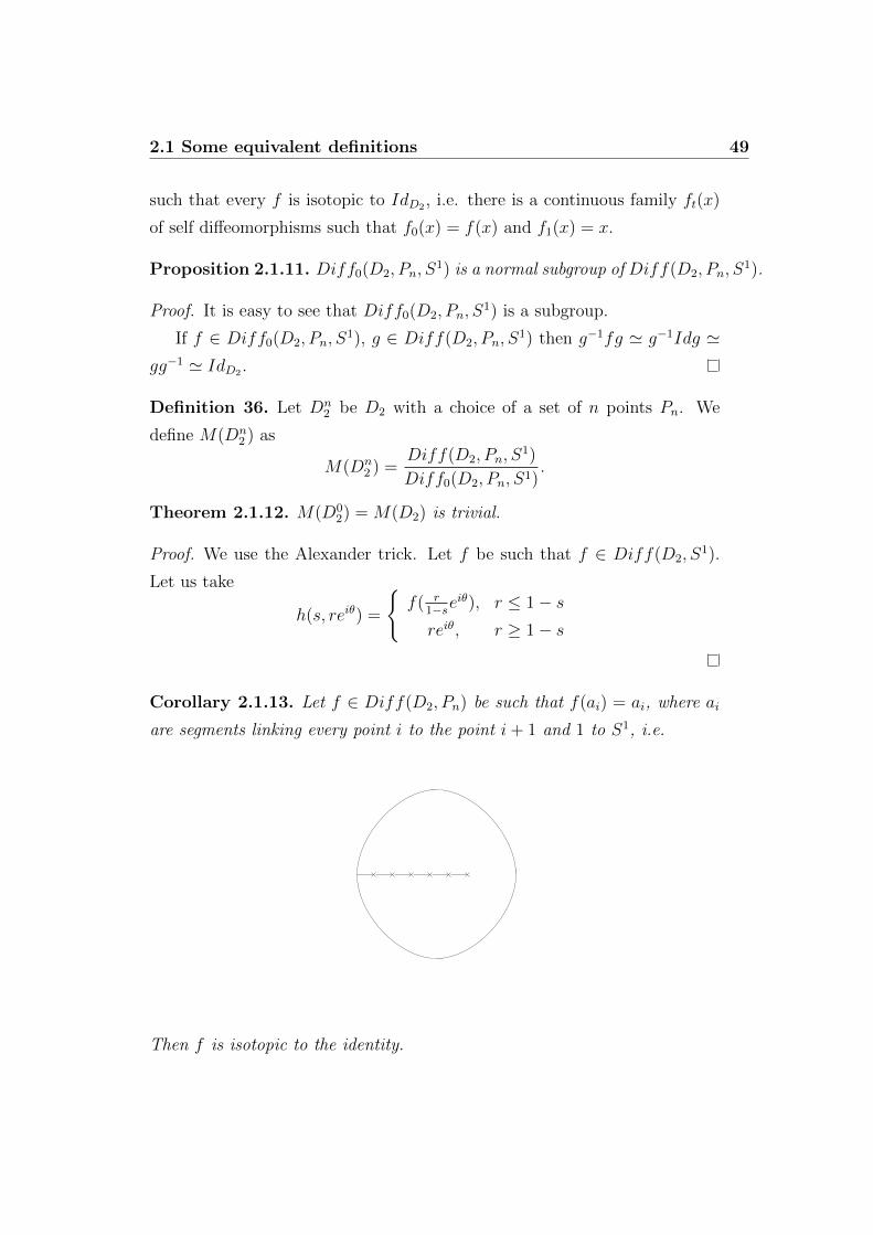
Corollary 2.1.13. Let f ∈ Diff(D2, Pn) be such that f(ai) = ai, where ai
are segments linking every point i to the point i+ 1 and 1 to S1, i.e.
Then f is isotopic to the identity.
50 2. Braid groups
Proof. If f is the identity on the segments, then it is isotopic to the identity in
a small open set U such that a1, . . . , an ⊂ U . (D2−Pn)−U is diffeomorphic
to D2, so we can apply theorem 2.1.12, f ' Id in (D2 − Pn) − U . Then
f ' Id in (D2 − Pn)− U .
We want now to find a group of generators for M(Dn2 ). We take n = 2,
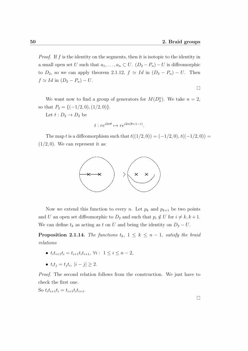
so that P2 = (−1/2, 0), (1/2, 0).Let t : D2 → D2 be
t : rei2πθ 7→ rei2π(θ+1−r).
The map t is a diffeomorphism such that t((1/2, 0)) = (−1/2, 0), t((−1/2, 0)) =
(1/2, 0). We can represent it as:
Now we extend this function to every n. Let pk and pk+1 be two points
and U an open set diffeomorphic to D2 and such that pi /∈ U for i 6= k, k+ 1.
We can define tk as acting as t on U and being the identity on D2 − U .
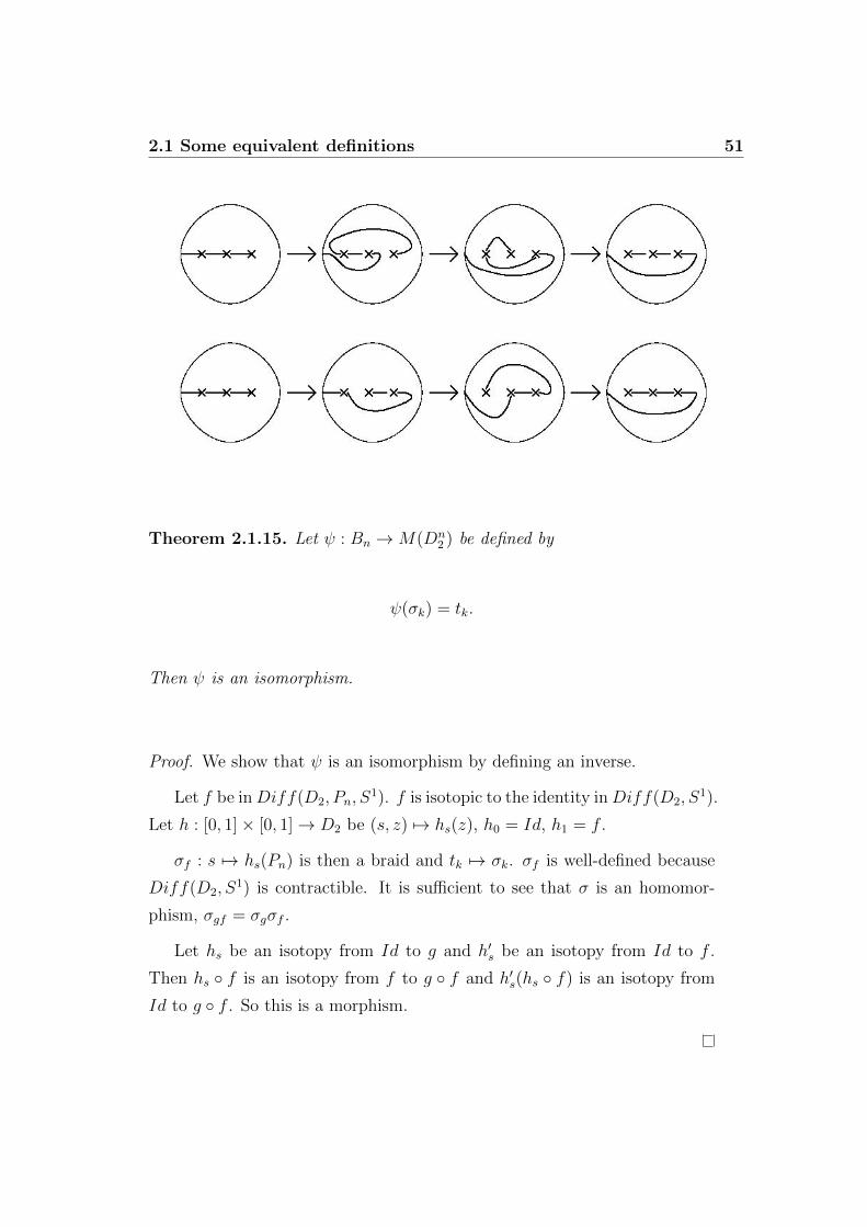
Proposition 2.1.14. The functions tk, 1 ≤ k ≤ n − 1, satisfy the braid
relations
• titi+1ti = ti+1titi+1, ∀i : 1 ≤ i ≤ n− 2,
• titj = tjti, |i− j| ≥ 2.
Proof. The second relation follows from the construction. We just have to
check the first one.
So titi+1ti = ti+1titi+1.
2.1 Some equivalent definitions 51
Theorem 2.1.15. Let ψ : Bn →M(Dn2 ) be defined by
ψ(σk) = tk.
Then ψ is an isomorphism.
Proof. We show that ψ is an isomorphism by defining an inverse.
Let f be inDiff(D2, Pn, S1). f is isotopic to the identity inDiff(D2, S
1).
Let h : [0, 1]× [0, 1]→ D2 be (s, z) 7→ hs(z), h0 = Id, h1 = f .
σf : s 7→ hs(Pn) is then a braid and tk 7→ σk. σf is well-defined because
Diff(D2, S1) is contractible. It is sufficient to see that σ is an homomor-
phism, σgf = σgσf .
Let hs be an isotopy from Id to g and h′s be an isotopy from Id to f .
Then hs f is an isotopy from f to g f and h′s(hs f) is an isotopy from
Id to g f . So this is a morphism.
52 2. Braid groups
2.2 Proprieties
2.2.1 Pure braid group
Let us focus on the projection π : Bn → Sn. The kernel of π is a group,
called the pure braid group Pn. Its elements are called pure braids on n
strands. A geometric braid on n strands represents an element in Pn if and
only if every strand starting by (i, 0, 0) ends in (i, 0, 1), ∀i : 1 ≤ i ≤ n.
We want to find a set of generators for this group. The group Pn is
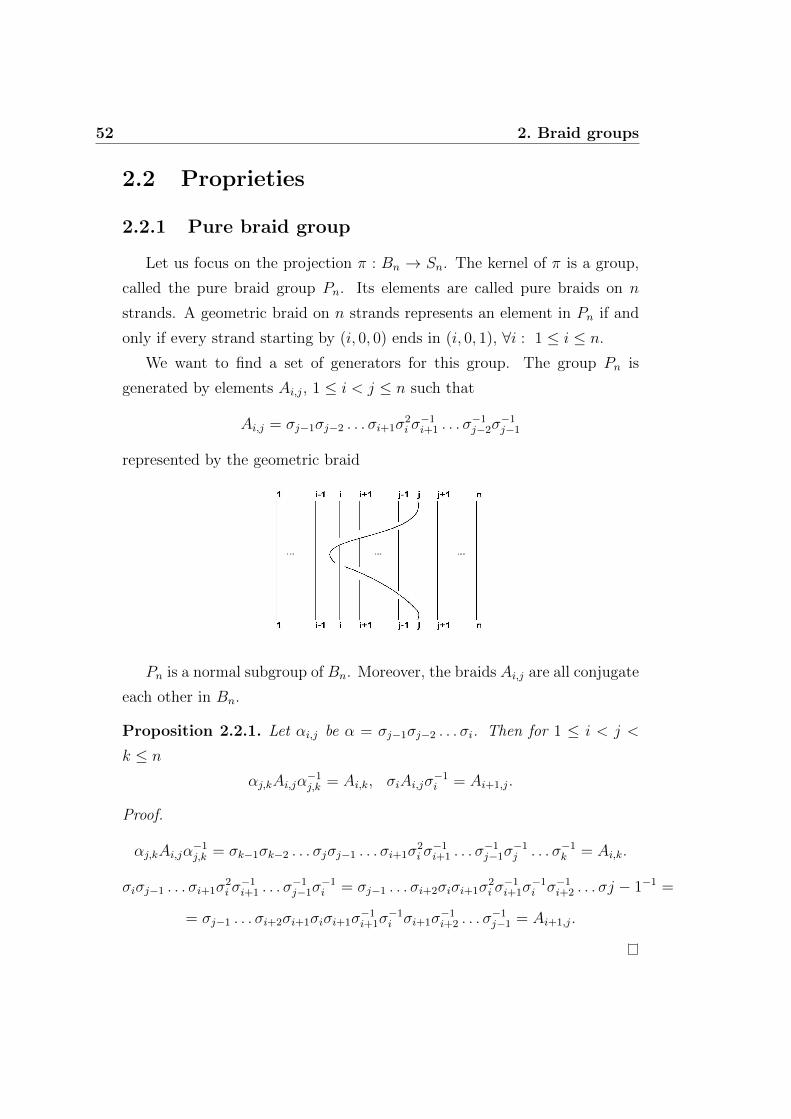
generated by elements Ai,j, 1 ≤ i < j ≤ n such that
Ai,j = σj−1σj−2 . . . σi+1σ2i σ−1i+1 . . . σ
−1j−2σ
−1j−1
represented by the geometric braid
Pn is a normal subgroup of Bn. Moreover, the braids Ai,j are all conjugate
each other in Bn.
Proposition 2.2.1. Let αi,j be α = σj−1σj−2 . . . σi. Then for 1 ≤ i < j <
k ≤ n
αj,kAi,jα−1j,k = Ai,k, σiAi,jσ
−1i = Ai+1,j.
Proof.
αj,kAi,jα−1j,k = σk−1σk−2 . . . σjσj−1 . . . σi+1σ
2i σ−1i+1 . . . σ
−1j−1σ
−1j . . . σ−1
k = Ai,k.
σiσj−1 . . . σi+1σ2i σ−1i+1 . . . σ
−1j−1σ
−1i = σj−1 . . . σi+2σiσi+1σ
2i σ−1i+1σ
−1i σ−1
i+2 . . . σj − 1−1 =
= σj−1 . . . σi+2σi+1σiσi+1σ−1i+1σ
−1i σi+1σ
−1i+2 . . . σ
−1j−1 = Ai+1,j.
2.2 Proprieties 53
Remark 30. The inclusion i : Bn → Bn+1 maps Pn to Pn+1, an homomor-
phism i|Pn : Pn → Pn+1. As in Bn, we can see this application geometrically
as the addiction of a vertical strand on the far right. Moreover, Pn → Pn+1
is injective.
We want now to define a forgetting homomorphism fn : Pn → Pn−1. Let
b be a pure braid. By definition, the i-th strand connects (i, 0, 0) to (i, 0, 1).
By convention, we eliminate the n-string.
Remark 31. If b is isotopic to b′, then fn(b) is isotopic to fn(b′).
By remark, the function fn is well defined from Pn to Pn−1 and it is a
group homomorphism.
Proposition 2.2.2. If i : Pn−1 → Pn is the natural inclusion and fn : Pn →Pn−1 is the forgetting homomorphism, then fn i = idPn−1.
The proposition easily follows from the geometric construction.
Corollary 2.2.3. i : Pn−1 → Pn is into and fn : Pn → Pn−1 is onto.
Let Un be ker(fn : Pn → Pn−1). There is an exact sequence
0→ U → Pn → Pn−1 → 0
There is a section i : Pn−1 → Pn, so the sequence splits and
Pn = Un o Pn−1.
Then every braid β ∈ Bn can be written as β = i(β′)βn, where β′ ∈ Pn−1
and βn ∈ U .
In particular, ker(Pn → Pn−1) = π1(C − z1, . . . , zn−1) = Fn−1, the free
group on n− 1 generator.
Iterating this construction, we obtain that Pn = Fn−1oFn−2o. . .oF2oF1,
so that
β = β2β3 . . . βn,
βi ∈ Ui ⊂ Pi.
54 2. Braid groups
Proposition 2.2.4. The group Pn admits a normal filtration
1 = U (0)n ⊂ U (1)
n ⊂ . . . ⊂ U (n−1)n = Pn
such that U(i)n /U
(i−1)n is a free group of rank n− i for all i.
Proof. Take U(0)n = 1 and
U (i)n = ker(fn−i+1 . . . fn−1fn : Pn → Pn−1)
for all i, 1 ≤ i ≤ n− 1. Then
U (i)n /U (i−1)
n ' ker(fn−i+1 : Pn−i+1 → Pn−i) = Un−i+1.
Corollary 2.2.5. The group Pn is torsion free.
Proof. The group Pn can be decomposed as semidirect product of free groups,
which are torsion free.
Theorem 2.2.6. The group Pn admits a presentation with n(n−1)2
generators
Ai,j, 1 ≤ i < j ≤ n and relations
A−1r,sAi,jAr,s =
Ai,j if s < i.
Ai,j if i < r < s < j.
Ar,jAi,jA−1r,j if s = i.
Ar,jAs,jAi,jA−1s,jA
−1r,j if i = r < s < j.
Ar,jAs,jA−1r,jA
−1s,jAi,jAs,jAr,jA
−1s,jA
−1r,j if r < i < s < j.
Proof. We have seen that Ai,j generate Pn. The relations can be proven
by drawing the diagrams. For example, for the second relation:
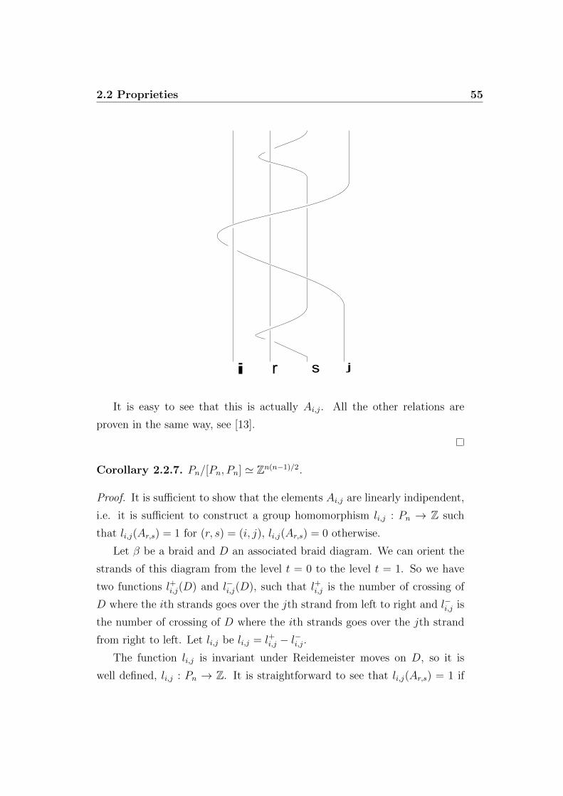
2.2 Proprieties 55
i r s j
It is easy to see that this is actually Ai,j. All the other relations are
proven in the same way, see [13].
Corollary 2.2.7. Pn/[Pn, Pn] ' Zn(n−1)/2.
Proof. It is sufficient to show that the elements Ai,j are linearly indipendent,
i.e. it is sufficient to construct a group homomorphism li,j : Pn → Z such
that li,j(Ar,s) = 1 for (r, s) = (i, j), li,j(Ar,s) = 0 otherwise.
Let β be a braid and D an associated braid diagram. We can orient the
strands of this diagram from the level t = 0 to the level t = 1. So we have
two functions l+i,j(D) and l−i,j(D), such that l+i,j is the number of crossing of
D where the ith strands goes over the jth strand from left to right and l−i,j is
the number of crossing of D where the ith strands goes over the jth strand
from right to left. Let li,j be li,j = l+i,j − l−i,j.The function li,j is invariant under Reidemeister moves on D, so it is
well defined, li,j : Pn → Z. It is straightforward to see that li,j(Ar,s) = 1 if
56 2. Braid groups
(r, s) = (i, j), 0 otherwise.
Definition 37. A group G is residually finite if for each g ∈ G− 1 there
is a homomorphism f from G to a finite group, f(g) 6= 1.
Proposition 2.2.8. Free groups are residually finite and a semidirect product
of two finitely generated residually finite groups is residually finite.
Proof. A proof of the first fact can be found in [18], while a proof of the
second can be found in [19].
Corollary 2.2.9. Bn is residually finite and so are all its subgroups.
Proof. We have seen that Pn is a semidirect product of free groups, so it
is residually finite. Moreover, every extension of a residually finite group
by a finite group is still residually finite, because the intersection of a finite
family of subgroups of finite index is a subgroup of finite index. Now, Bn is
an extension of Pn by Sn, which is a finite group, so that Bn is residually
finite too. It is easy to see that every subgroup of a residually finite group is
residually finite.
Corollary 2.2.10. f in : Pn → Pn−1 is defined as the map forgetting the ith
string, for i = 1, 2 . . . , n. The kernel of f in is a free group of rank n− 1 with
free generators Ai,1, . . . , Ai−1,i, Ai,i+1, . . . , Ai,n.
Proof. Let αi,n be α = σn−1σn−2 . . . σi and let β be a pure braid in Pn. We
take into consideration the braid αi,nβα−1i,n
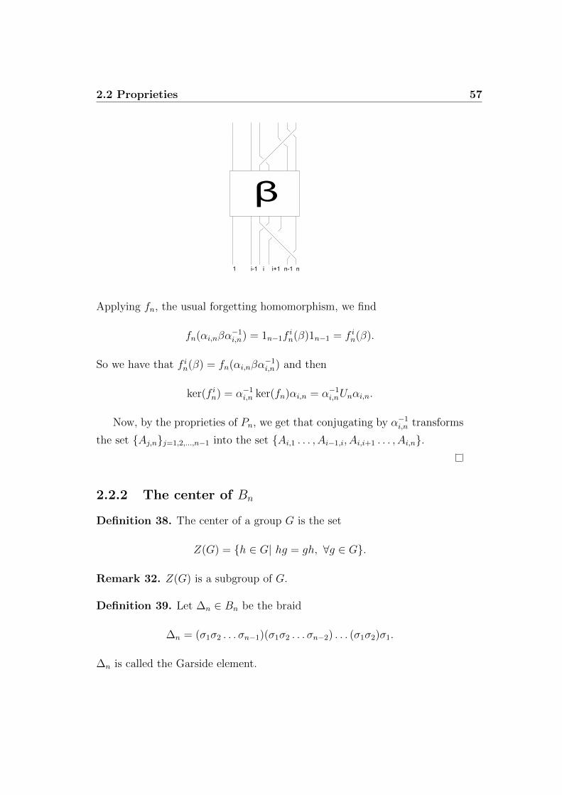
2.2 Proprieties 57
1 i-1 i i+1 nn-1
β
Applying fn, the usual forgetting homomorphism, we find
fn(αi,nβα−1i,n) = 1n−1f
in(β)1n−1 = f in(β).
So we have that f in(β) = fn(αi,nβα−1i,n) and then
ker(f in) = α−1i,n ker(fn)αi,n = α−1
i,nUnαi,n.
Now, by the proprieties of Pn, we get that conjugating by α−1i,n transforms
the set Aj,nj=1,2,...,n−1 into the set Ai,1 . . . , Ai−1,i, Ai,i+1 . . . , Ai,n.
2.2.2 The center of Bn
Definition 38. The center of a group G is the set
Z(G) = h ∈ G| hg = gh, ∀g ∈ G.
Remark 32. Z(G) is a subgroup of G.
Definition 39. Let ∆n ∈ Bn be the braid
∆n = (σ1σ2 . . . σn−1)(σ1σ2 . . . σn−2) . . . (σ1σ2)σ1.
∆n is called the Garside element.
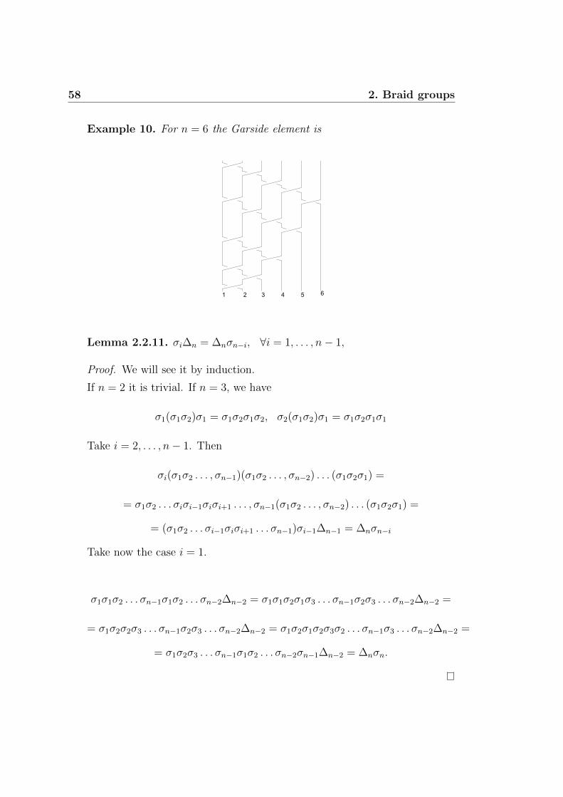
58 2. Braid groups
Example 10. For n = 6 the Garside element is
1 2 3 4 5 6
Lemma 2.2.11. σi∆n = ∆nσn−i, ∀i = 1, . . . , n− 1,
Proof. We will see it by induction.
If n = 2 it is trivial. If n = 3, we have
σ1(σ1σ2)σ1 = σ1σ2σ1σ2, σ2(σ1σ2)σ1 = σ1σ2σ1σ1
Take i = 2, . . . , n− 1. Then
σi(σ1σ2 . . . , σn−1)(σ1σ2 . . . , σn−2) . . . (σ1σ2σ1) =
= σ1σ2 . . . σiσi−1σiσi+1 . . . , σn−1(σ1σ2 . . . , σn−2) . . . (σ1σ2σ1) =
= (σ1σ2 . . . σi−1σiσi+1 . . . σn−1)σi−1∆n−1 = ∆nσn−i
Take now the case i = 1.
σ1σ1σ2 . . . σn−1σ1σ2 . . . σn−2∆n−2 = σ1σ1σ2σ1σ3 . . . σn−1σ2σ3 . . . σn−2∆n−2 =
= σ1σ2σ2σ3 . . . σn−1σ2σ3 . . . σn−2∆n−2 = σ1σ2σ1σ2σ3σ2 . . . σn−1σ3 . . . σn−2∆n−2 =
= σ1σ2σ3 . . . σn−1σ1σ2 . . . σn−2σn−1∆n−2 = ∆nσn.
2.2 Proprieties 59
Corollary 2.2.12. Let θn be θn = ∆2n. Then σiθn = θnσi. Moreover, θn =
i(θn−1)γn, where
γn = A1,nA2,n . . . An−1,n
and i : Pn−1 → Pn is the natural inclusion.
Theorem 2.2.13. Z(Bn) = Z(Pn) is the infinite cyclic group generated by
θn.
Proof. We have seen that θn ∈ Z(Bn). We should prove that every element
of Z(Bn) is a power of θn. We start by focusing on P2.
For n = 2 it is obvious, because P2 is the infinite cyclic group generated
by σ21 = θ2.
Let now β be in Z(Pn), n ≥ 3. We can decompose β as β = i(β′)βn,
β′ = fn(β) ∈ Pn−1 and β ∈ Un. We can notice that the braid γn commutes
with any elements of i(Pn−1). Moreover, β commutes with γ, because we
have supposed β ∈ Z(Pn). So γ commutes with βn = i(β′)−1β and the group
G generated by γ and βn is an abelian group, G ⊂ Un. Un is a free group, so
all its subgroups are free groups too. This implies that G is an infinite cyclic
group.
Let li,j : Pn → Z be the homomorphism defined in Corollary 2.2.7.
l1,n(γ) = 1, so γ is a generator of G and ∃k : βn = γk. By the induc-
tion assumption there is m such that β′ = fn(β) = (θmn−1). Then we have
li,n = k ∀i = 1, 2, . . . , n−1, so it is independent from i. Since β ∈ Z(Pn), also
σn−1βσ−1n−1 ∈ Z(Pn) and li,n(σn−1βσ
−1n−1) is independent from i. By definition
we obtain
l1,n(σn−1βσ−1n−1) = l1,n−1(β) = m.
ln−1,n(σn−1βσn−1) = ln−1,n(β) = k.
and m = k and β = i(θn−1γ)k = θkn.
For n ≥ 3 the center of Bn projects to the trivial subgroup of Sn, because
Z(Sn) = 1. So Z(Bn) ⊂ Z(Pn). Since θn ∈ Z(Bn), Z(Bn) = (θn).
60 2. Braid groups
Corollary 2.2.14. Bm and Bn are isomorphic if and only if m = n.
Proof. The image of Z(Bn) in Bn/[Bn, Bn] is a subgroup of Z of index n(n−1). If Bn is isomorphic to Bm then m(m− 1) = n(n− 1), so that m = n.
2.2.3 Homotopy groups
Theorem 2.2.15. Let (Sn, s0) and (X, xo) be two topological pointed spaces.
Let πn(X, x0) be the set of homotopy classes of maps f : Sn → X such
that f(s0) = x0. Then πx(X, x0) is a group, called the n-homotopy group of
(X, x0).
Proof. A proof can be found in every book of algebraic topology, see [14] or
[7].
Proposition 2.2.16. πn(X, x0) is a commutative group for n ≥ 2.
Definition 40. A map p : E → X is locally trivial if and only if ∀x ∈ X there
is a neighbourhood V = Vx and a homeomorphism p−1(V )∼→ p−1(x) × V
such that there is a commutative diagram
p−1(V )∼→ p−1(x)× V
↓ ↓V → V
Theorem 2.2.17. Let p : E → X, X arc connected, be a locally trivial
fibration. Let e0 be in E, p(e0) = b0, F = p−1(b0) and f0 ∈ F . There is a
long exact sequence in homotopy:
. . .→ πn(F, f0)→ πn(E, e0)→ πn(X, x0)→ πn−1(F, f0)→ . . .→ π1(F, f0)
→ π1(E, e0)→ π1(X, x0)→ π0(F, f0)→ π0(E, e0)→ π0(X, x0)→ 0.
A proof can be found in [14].
Corollary 2.2.18. If p is a covering map, then πn(F ) = 0 for n ≥ 2 and
πn(E) ' πn(X) for n ≥ 2
2.3 Representation of links by braids 61
Corollary 2.2.18 follows from theorem 2.2.17 by setting πn(F ) = 0 in the
long exact sequence.
Let us now focus on the configuration spaces. There is a map
p : Cn −∆n → Cn−1 −∆n−1
such that p((z1, . . . , zn)) = (z1, . . . , zn−1), so that
p−1((q1, . . . , qn)) = C−Qn−1
where Qn−1 = q1, . . . , qn−1. The map p is locally trivial.
Theorem 2.2.19. πk(Confn(C)) = 0 for k ≥ 2, n ≥ 1.
Proof. We apply theorem 2.217 and corollary 2.2.18. F = C − Qn−1 ∼∨n−1i=1 S
i, so πk(F ) = 0 for k ≥ 2.
We prove it by induction of n. For n = 1, Conf1(C) = C and so we have
the claim.
For n > 1 we take the sequence:
. . .→ πk(F )→ πk(Cn −∆n)→ πk(Cn−1 −∆n−1)→ . . .
By induction, πk(Cn−1 − ∆n−1) = 0 for k ≥ 2 and we have seen that
πk(Cn−1 −∆n−1) = 0, so that πk(Confn(C)) = 0 for k ≥ 2.
2.3 Representation of links by braids
2.3.1 Construction of links by braids
Definition 41. Let L be a link in the solid torus T = D2 × S1. L is called
a closed n-braid if L meets each 2-disk D2 × z, z ∈ S1, transversely in n
points.
Remark 33. The projection V → S1 restricted to L gives a n-fold covering
L→ S1.
62 2. Braid groups
We provide L with the canonical orientation obtained by lifting the coun-
terclockwise orientation of S1.
Definition 42. Two closed braids in V are isotopic if they are isotopic as
oriented links.
Remark 34. A link in V does not need to be isotopic to a closed braid in
V , as for example a link lying inside a small 3-ball in V .
Such links are called closed n-braid because, given a braid β on n strands,
there is a standard way to obtain from it a closed n-braid in the solid torus
V . A solid torus can be seen as the cylinder D2 × I with identifications
(x, 0) ∼ (x, 1). So, given a braid β, take the geometric braid b ⊂ D2 × I.
Then b, image of b in the projection D2 × I → V , is a closed n-braid in V .
Proposition 2.3.1. Let β be a n-braid and b a geometric braid associated
to β. The isotopy class of b depends only on β.
Proof. Let b and b′ be two geometric braids in D2×I. Then b is isotopic to b′,
i.e. there is an isotopy of D×I constant on the boundary and transforming b
in b′. This isotopy induces an isotopy between b and b′ in V , thus the isotopy
class of b does not depend on the choice of the geometric braid.
Theorem 2.3.2. For any n ≥ 1 and any β and β′ ∈ Bn with geometric
braids b and b′, the closed braids b and b′ are isotopic in the solid torus if and
only if β and β′ are conjugate in Bn.
Proof. A proof can be found in [16].
Definition 43. Let β be a braid diagram. The closure β of β is the link
diagram obtained by joining the bottom endpoints with the top endpoints
by n standard arcs. We call the oriented link which diagram is β as β too.
Proposition 2.3.3. Two closed braid diagrams D and D′ in S1×I represent
isotopic closed braids in the solid torus S1 × I × I if and only if D can be
transformed in D′ by a finite sequence of isotopies and Reidemeister moves.
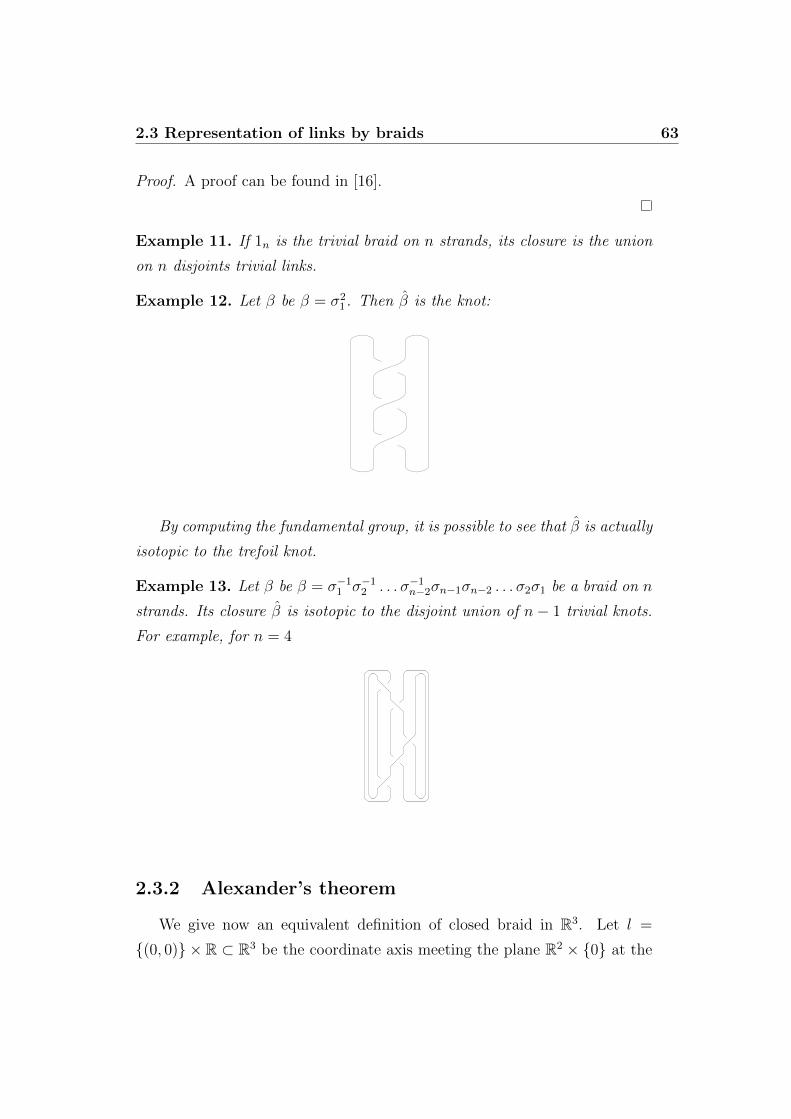
2.3 Representation of links by braids 63
Proof. A proof can be found in [16].
Example 11. If 1n is the trivial braid on n strands, its closure is the union
on n disjoints trivial links.
Example 12. Let β be β = σ21. Then β is the knot:
By computing the fundamental group, it is possible to see that β is actually
isotopic to the trefoil knot.
Example 13. Let β be β = σ−11 σ−1
2 . . . σ−1n−2σn−1σn−2 . . . σ2σ1 be a braid on n
strands. Its closure β is isotopic to the disjoint union of n− 1 trivial knots.
For example, for n = 4
2.3.2 Alexander’s theorem
We give now an equivalent definition of closed braid in R3. Let l =
(0, 0) × R ⊂ R3 be the coordinate axis meeting the plane R2 × 0 at the
64 2. Braid groups
origin O = (0, 0, 0). We can choose a positive direction of rotation about l
as the counterclockwise direction about O in the plane R2 × 0.
Definition 44. An oriented geometric link L ⊂ R3 − l is a closed n-braid if
the vector from O to any point X ∈ L rotates in the positive direction about
l when X moves along L in the direction determined by the orientation of L.
Lemma 2.3.4. The two definitions are equivalent.
Proof. Let D2 be a disk lying in an open half-plane bounded by l in R3 and
having its center in R2 × 0. Now, rotating D around l we obtain a solid
torus V = D2 × S1. The assumption then follows by considering that, if D
is big enough, a given link L ⊂ R3 − l lies in V .
Theorem 2.3.5. Any oriented link in R3 is isotopic to a closed braid.
Proof. Any link in R3 is isotopic to a polygonal link, so it is sufficient to
prove the theorem for such links. By moving the vertices of L we can assume
that L ⊂ R3− l, where l = (0, 0)×R, and that the edges of L do not lie in
planes containing the axis l. Let AC be an edge of L, labeling the vertices
such that L is oriented from A to C. The edge AC is said to be positive
(resp. negative) if the vector from the origin 0 ∈ l to a point X ∈ AC rotates
in the positive (resp. negative) direction about l when X moves from A to
C. By the assumption that AC does not lie in a plane containing l, AC is
necessarily positive or negative. The edge AC is now said to be accessible if
there is a point B ∈ l such that the triangle ABC meets L only along AC.
If all edges of L are positive, L is a closed braid.
Let AC be a negative edge of L. It is possible to replace AC with a
sequence of positive edges. Assume AC is accessible. Then there exists
B ∈ l such that the triangle ABC meets L only along AC. In the plane
containing ABC we take a bigger triangle AB′C containing B in its interior,
meeting l only at B and meeting L only along AC.
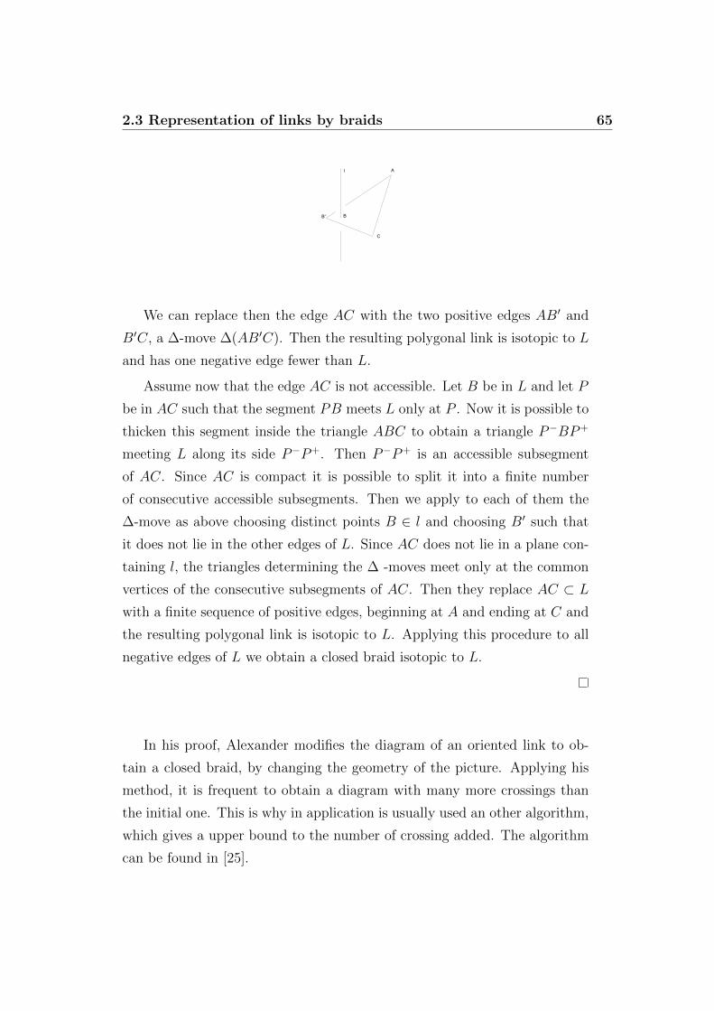
2.3 Representation of links by braids 65
B
A
C
B'
l
We can replace then the edge AC with the two positive edges AB′ and
B′C, a ∆-move ∆(AB′C). Then the resulting polygonal link is isotopic to L
and has one negative edge fewer than L.
Assume now that the edge AC is not accessible. Let B be in L and let P
be in AC such that the segment PB meets L only at P . Now it is possible to
thicken this segment inside the triangle ABC to obtain a triangle P−BP+
meeting L along its side P−P+. Then P−P+ is an accessible subsegment
of AC. Since AC is compact it is possible to split it into a finite number
of consecutive accessible subsegments. Then we apply to each of them the
∆-move as above choosing distinct points B ∈ l and choosing B′ such that
it does not lie in the other edges of L. Since AC does not lie in a plane con-
taining l, the triangles determining the ∆ -moves meet only at the common
vertices of the consecutive subsegments of AC. Then they replace AC ⊂ L
with a finite sequence of positive edges, beginning at A and ending at C and
the resulting polygonal link is isotopic to L. Applying this procedure to all
negative edges of L we obtain a closed braid isotopic to L.
In his proof, Alexander modifies the diagram of an oriented link to ob-
tain a closed braid, by changing the geometry of the picture. Applying his
method, it is frequent to obtain a diagram with many more crossings than
the initial one. This is why in application is usually used an other algorithm,
which gives a upper bound to the number of crossing added. The algorithm
can be found in [25].
66 2. Braid groups
2.3.3 Markov theorem
We have a method for building a link diagram as a closed braid. Now
we want to investigate the other problem: how to describe all braids with
isotopic closures in R3.
We have seen that if two braids β and β′ are conjugate then they have
isotopic closures, but the converse is not true.
Example 14. Let us take σ1, σ−11 ∈ B2. They are not conjugate each to the
other, but their closures are both isotopic to the trivial knot.
Example 15. Let i : Bn → Bn+1 be the natural embedding of Bn in Bn+1.
Let β be a braid in Bn. Then the braids σni(β) and σ−1n i(β) have isotopic
closures. Also, their closures are isotopic to β.
Definition 45. Two braids β and β′ are said to be M-equivalent if they can
be related by a finite sequence of moves M1 and M2, and their inverses, given
by
1. if β, γ ∈ Bn, β 7→ γβγ−1;
2. if β ∈ Bn, i : Bn → Bn+1 is the canonical embedding, β 7→ σ±1n i(β).
The moves M1 and M2 are called Markov moves.
Remark 35. The relation of M-equivalence is an equivalence relation.
Remark 36. Two braids can be M-equivalent also if they have a different
number of strands.
Example 16. Let us show that the braids σ1 and σ−11 ∈ B2 are equivalent.
σ1 ∼ σ−12 σ1 ∼ (σ1σ2)−1(σ−1
2 σ1)(σ1σ2) =
= σ−11 σ−1
2 σ−11 σ2
1σ2 = σ−11 σ−1
2 σ1σ2 =
= σ2σ−11 σ−1
2 σ2 = σ2σ−11 ∼ σ−1
1 .
2.3 Representation of links by braids 67
Theorem 2.3.6. Two braids have isotopic closures in R3 if and only if they
are M-equivalent.
Proof. A proof can be found in [16].
Corollary 2.3.7. Let Λ be the set of all isotopy classes of nonempty oriented
links in R3. The mapping∐
n≥1Bn → Λ assigning to a braid the isotopy class
of its closure induces a bijection from the quotient set(∐
n≥1Bn)
∼∼→ Λ.
From corollary 2.3.7, it is possible to define functions acting on braids
and such that they are well defined on their closures, i.e. on links.
Definition 46. A Markov function with values in a set E is a sequence of
functions fn : Bn → En≥1, satisfying the following conditions:
1. ∀ n ≥ 1 and ∀ α, β ∈ Bn,
fn(β) = fn(α−1βα)
2. ∀ n ≥ 1 and all β ∈ Bn,
fn(β) = fn+1(σni(β)), fn(β) = fn+1(σ−1n (β)).
Proposition 2.3.8. Any Markov function fn : Bn → En≥1 determines an
E-valued isotopy invariant f of oriented links in R3.
Proof. Let L be an oriented link in R3. For Alexander theorem, it is possible
to take a braid β ∈ Bn such that L is isotopic to β. Let f(L) be f(L) = fn(β).
Let β′ be another braid whose closure is isotopic to L. β and β′ are M-
equivalent, so there is a finite sequence of Markov moves starting from β′
and ending in β. By definition the Markov functions are invariant on M-
moves, so the function f is well defined. Let now L′ be an oriented link
isotopic to L. Let β ∈ Bn be a braid whose closure is isotopic to L. Then
the closure of β is also isotopic to L′ and f(L) = fn(β) = f(L′).
68 2. Braid groups
2.4 Representations of braid groups
2.4.1 The Burau representation
Definition 47. Let us take n ≥ 2. For i = 1, . . . , n−1 we take the following
n× n matrix over the ring Λ = Z[t±]:
Ui =
Ii−1 0 0 0
0 1− t t 0
0 1 0 0
0 0 0 In−i−1
.
where Im denotes the unit m×m matrix. If i = 1 the first matrix disappears,
and so does the second if i = n− 1.
Remark 37. For t = 1 the matrices Ui become the permutation matrices.
Proposition 2.4.1. The matrix Ui is invertible with inverse given by
U−1i =
Ii−1 0 0 0
0 0 1 0
0 t−1 1− t−1 0
0 0 0 In−i−1
.
Proposition 2.4.2. The matrices Ui, i = 0, . . . , n − 1 satisfy the following
proprieties:
1. UiUj = UjUi, ∀i, j = 0, . . . , n− 1 : |i− j| ≥ 2,
2. UiUi+1Ui = Ui+1UiUi+1, ∀i = 0, . . . , n− 2.
Proof. These two propositions are proven by direct computation.
It is possible to define a group homomorphism ψn : Bn → GLn(Λ), n ≥ 2,
by ψn(σi) = Ui. By proposition 2.4.1 and proposition 2.4.2 this is well
defined.

2.4 Representations of braid groups 69
Definition 48. The map ψn : Bn → GLn(Λ) such that ψn(σi) = Ui is called
the Burau representation of Bn.
Remark 38. The Burau representations ψnn≥1 are compatible with the
natural inclusions i : Bn → Bn+1 for any β ∈ Bn, i.e.
ψn+1(i(β)) =
(ψn(β) 0
0 1
).
Definition 49. A group homomorphism ϕ : G→ G′ is said to be faithful is
its kernel is trivial.
Theorem 2.4.3. The Burau representation ψn is faithful for n = 2, 3,
unfaithful for n ≥ 5.
Proof. ker(ψn) ⊂ ker(ψn+1). Then it is sufficient to prove the unfaithfulness
for n = 5. This can be made by showing a non-trivial element in Bn such
that his image in GLn(Λ) is 0. Set
γ = σ4σ−13 σ−1
2 σ21σ−12 σ−2
1 σ−22 σ−1
1 σ−54 σ2σ3σ
34σ2σ
21σ2σ
−13
Then the commutator ρ = [γσ4σ−1, σ4σ3σ2σ
21σ2σ3σ4] is a non trivial ele-
ment in ker(ψ5) ⊂ B5.
Let us see the case n = 2, B2 ' Z. Then it is sufficient to see that Un 6= I2
∀n ∈ Z0. We have (1,−1)U = (−t, t) = −t(1,−1). Then (1,−1)Uk =
tk(1,−1) for all k ∈ Z. Then Uk 6= Uh for k 6= h and < U >= Z.
The proof for the case n = 3 can be found in [16].
Remark 39. The vector (1, 1, . . . , 1) is an eigenvector for every matrix Ui.
By remark 39, it is possible to decompose the representation matrix in
a direct sum of a 1-dimensional representation and of a n − 1-dimensional
representation. Let P be the matrix
P =
1 1 . . . 1
0 1 . . . 1...
. . . . . ....
0 . . . 0 1

70 2. Braid groups
Then P−1UiP is the matrix
(Ui 0
0 1
), where Ui is the matrix, for 1 <
i < n− 1
Ui =
Ii−2 0 0 0 0
0 1 t 0 0
0 0 −t 0 0
0 0 1 1 0
0 0 0 0 In−i−2
For i = 1 and i = n− 1 the matrix is
U1 =
−t 0 0
1 1 0
0 0 In−3
Ui =
In−3 0 0
0 1 t
0 0 −t
The group homomorphism ψn : Bn → GLn−1(Λ) such that ψn(σi) = Ui
is called the reduced Burau representation.
2.4.2 A homological description of the Burau repre-
sentation
We want now to understand the geometric meaning of the Burau repre-
sentation. To do that, we shall remember that braid groups can be defined
as mapping class groups on punctured disks, as it has been done in 2.1.4.
Remark 40. H1(D2 − x) = Z, generated by the class of loops encircling
x in counterclockwise direction. Each loop represents k times the generator,
where k is the winding number of the loop around x.
Remark 41. Hn(D2 − Pn) = Zn, where Pn are n distinct points. The
generators are the classes of small loops encircling only one point in Pn in
the counterclockwise direction.
Definition 50. Let γ be a loop in D2 − Pn. We define the total winding
number of γ as the sum of its winding numbers around x1, . . . , xn. The total
winding number defines a homomorphism H1(Dn)→ Z.
2.4 Representations of braid groups 71
Let Dn → Dn be the regular covering corresponding to the homomor-
phism H1(Dn)→ Z such that (k1, . . . , kn) 7→ k1 + . . . + kn. Then the group
of covering transformations of Dn is Z, a multiplicative group with generator
t. Thus the group H1(Dn) acquires the structures of a Λ-module.
Let d ∈ ∂D be a basepoint for Dn. Any diffeomorphism d : Dn → Dn
lifts uniquely to a diffeomorphism h : Dn → Dn which fixes the fiber over
d pointwise. Thus there is an induced homomorphism Bn → Aut(H1(Dn))
defined by h→ h∗, where h∗ is a Λ-linear automorphism of H1(Dn). We will
see that this map is equivalent to the reduced Burau representation.
Definition 51. Let α, β be two embedded arcs in Dn with endpoints in the
set Pn, n ≥ 4. Let α, β be lifts of α and β to Dn. Then
< α, β >=∑k∈Z
(tkα · β)tk ∈ Λ
where (tkα · β) is the algebraic intersection of the arcs tkα and β in Dn. This
intersection is also called Blanchfield intersection.
Remark 42. The sum is finite and it is defined up to multiplication by a
power of t depending on the choices of the lifts α and β.
Now, to compute < α, β > it is possible to deform α with respect to β
and compute the geometric intersection. We call εp the intersection sign of
the two loops at an intersection point p ∈ α∩β. We determine also a number
kp ∈ Z by the following. Let us take two points p, q ∈ α ∩ β. Then kp − kqis the total winding number of the loop going from p to q along α and then
from q to p along β. Then
< α, β >=∑p∈α∩β
εptkp
For 1 ≤ j ≤ n let aj be the oriented segment joining qj and qj+1, where
qi are points in Pn. Let us link aj to the point (−1, 0) ∈ D2 that we take as
basepoint. For all j let bj be a vertical segment, oriented downward, passing
for the middle of aj. Let aj and bj be their lifts.
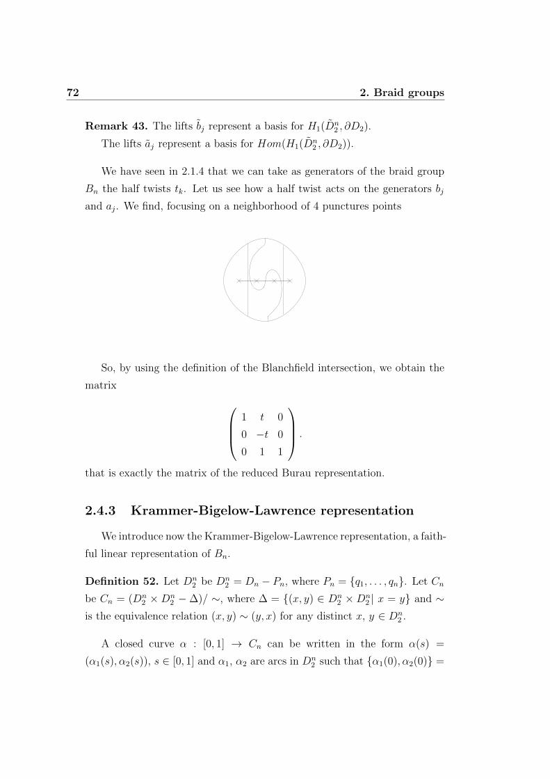
72 2. Braid groups
Remark 43. The lifts bj represent a basis for H1(Dn2 , ∂D2).
The lifts aj represent a basis for Hom(H1(Dn2 , ∂D2)).
We have seen in 2.1.4 that we can take as generators of the braid group
Bn the half twists tk. Let us see how a half twist acts on the generators bj
and aj. We find, focusing on a neighborhood of 4 punctures points
So, by using the definition of the Blanchfield intersection, we obtain the
matrix 1 t 0
0 −t 0
0 1 1
.
that is exactly the matrix of the reduced Burau representation.
2.4.3 Krammer-Bigelow-Lawrence representation
We introduce now the Krammer-Bigelow-Lawrence representation, a faith-
ful linear representation of Bn.
Definition 52. Let Dn2 be Dn
2 = Dn − Pn, where Pn = q1, . . . , qn. Let Cn
be Cn = (Dn2 ×Dn
2 −∆)/ ∼, where ∆ = (x, y) ∈ Dn2 ×Dn
2 | x = y and ∼is the equivalence relation (x, y) ∼ (y, x) for any distinct x, y ∈ Dn
2 .
A closed curve α : [0, 1] → Cn can be written in the form α(s) =
(α1(s), α2(s)), s ∈ [0, 1] and α1, α2 are arcs in Dn2 such that α1(0), α2(0) =
2.4 Representations of braid groups 73
α1(1), α2(1). Thus the arcs α1 and α2 are either loops or can be composed
one with the other.
Remark 44. The curves α = (α1, α2) form a closed oriented one-manifold
γ mapped to Dn2 .
Let a(α) ∈ Z be the total winding number of γ around the points
q1, . . . , qn. For the construction of the space, α1(s) 6= α2(s) ∀s ∈ [0, 1].
Then it is well defined the map
s 7→ α1(s)− α2(s)
|α1(s)− α2(s)
Composing this map with the projection S1 → RP 1 we obtain a loop in
RP 1. We call b(α) the corresponding element in H1(RP 1). So we have a
map ψ : H1(C)→ Z[q±1, t±1] such that α 7→ qa(α)tbα.
There is a regular covering C → C associated to the kernel of ψ, so that
the generators q, t acts on C as commuting covering transformations. Now
any diffeomorphism h of Dn2 induces a diffeomorphism C → C by h(x, y) =
hx, hy. We denote this diffeomorphism with h too. The diffeomorphism h
lifts to a map h : C → C. Thus there is a representation Bn → Aut(H2(C))
such that [h] ∈ Bn maps to the automorphism h∗ of H2(C).
Theorem 2.4.4. The representation Bn → Aut(H2(C)) is faithful for all
n ≥ 1.
Proof. A proof can be found in [16] or in [26].
The proof consists in a homological construction, as it has been done for
the Burau representation. This construction is far more complicated, but it
allows to prove that braid groups are linear, a statement really difficult to
prove only with algebraic methods.

74 2. Braid groups
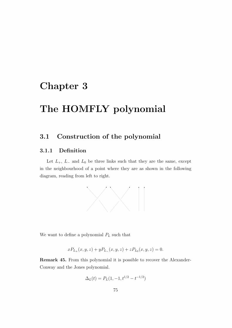
Chapter 3
The HOMFLY polynomial
3.1 Construction of the polynomial
3.1.1 Definition
Let L+, L− and L0 be three links such that they are the same, except
in the neighbourhood of a point where they are as shown in the following
diagram, reading from left to right.
We want to define a polynomial PL such that
xPL+(x, y, z) + yPL−(x, y, z) + zPL0(x, y, z) = 0.
Remark 45. From this polynomial it is possible to recover the Alexander-
Conway and the Jones polynomial.
∆L(t) = PL(1,−1, t1/2 − t−1/2)
75
76 3. The HOMFLY polynomial
VL(t) = PL(t,−t−1, t1/2 − t−1/2)
Moreover, being an homogeneous polynomial in 3 variables, it is possible
to take it as a non-homogeneous polynomial in two variables. In literature
usually it is taken the polynomial PL(l,m) = PL(l, l−1,m), so the relation
becomes:
lPL+1(l,m) + l−1PL−1 +mPL0 = 0
Theorem 3.1.1. There is a unique function
P : Oriented links in S3 → Z[l±,m±]
well defined up to isotopy such that P (unknot) = 1 and
lPL+(l,m) + l−1PL−(l,m) +mPL0 = 0
We will see a proof in the next section. Other proofs of theorem 3.1.1 can
be found in [12] or in [17].
Definition 53. Given an integer N > 1, we call invariant of type AN the
polynomial satisfying:
• PN(unknot) = 1
• q(N+1)/2PN(L+1)− q−(N+1)/2PN(L−1) = (q1/2 − q−1/2)PN(L0)
In the following chapters we will build a homological definition for this
invariant.
There is a theorem claiming that it is possible to reconstruct the HOM-
FLY polynomial by the values of the invariant of type AN , see [21] or [24]
for a more complete explanation. This is why we can say that we are able to
construct a general homological definition for the HOMFLY polynomial.
3.1 Construction of the polynomial 77
3.1.2 Construction by Hecke algebra
Proposition 3.1.2. The symmetric group Sn admits a presentation
Sn =< τ1, . . . , τn−1| 1, 2, 3 >
where τi = (i i+ 1) and
1. τ 2i = 1, ∀ i : 1 ≤ i ≤ n− 1,
2. τiτj = τjτi, ∀ i, j : 1 ≤ i < j − 1 ≤ n− 2,
3. τiτi+1τi = τi+1τiτi+1, ∀ i : 1 ≤ i ≤ n− 2.
The group operation in Sn is written from left to right, so that for example
(1 2)(2 3) = (1 3 2)
Proof. A proof can be found in every book of algebra, for example [1].
Remark 46. It is possible to identify Sn−1 with the subgroup of permuta-
tions in Sn leaving n fixed.
Definition 54. Given a permutation π ∈ Sn such that π(n) = j, we define
bπ(τi) = (j j + 1)(j + 1 j + 2) . . . (n− 1 n) · bπ′(τi)
where π′ ∈ Sn−1.
Proposition 3.1.3. Let Wn be Wn = bπ(τi)|π ∈ Sn. The elements of Wn
satisfy the Schreier condition:
• if bπ(τi) = w(τi)τk then w(τi) = bπ·τ−1k
(τi),
• bid is the empty word.
Also, bπ(τi) are of minimal length and τn−1 occurs at most once in each
bπ(τi) ∈ Wn.
Proof. A proof can be found in [8].

78 3. The HOMFLY polynomial
Definition 55. Sn =< τ1, τ2, . . . , τn−1| 1, 2 > where
1. τiτj = τj τi, ∀ i, j : 1 ≤ i < j − 1 ≤ n− 2,
2. τiτi+1τi = τi+1τiτi+1, ∀ i : 1 ≤ i ≤ n− 2
and such that inverses are not allowed. Then Sn is a semigroup.
There is a canonical homomorphism k : Sn → Sn such that k(τi) = τi.
Let bπ and Wn be respectively bπ = bπ(τi) and Wn = bπ | π ∈ Sn.We should see now what happens to the products bπ τk = bρ. There are
two cases:
1. the class of bπ τk contains a representative bρ ∈ Wn
2. the class of bπ τk does not contain a representative bρ ∈ Wn
Remark 47. The first case occurs when the strings crossing at τk do not
cross in bπ, ρ = πτk. In the second case they do and bπ τk = bρτ2k , so that
bπ · τk =
bρ, ρ = πτk
bρτ2k , ρτk = π
Let Mn be a free module of rank n! over a unitary commutative ring R
using the n! words of Wn. We take the generator ci instead of τi, 1 ≤ i ≤ n−1
and we take w(ci) = w′ci if and only if w(τi) = w(τi). Let Mn be the free
R-module with basis Wn(ci) = bπ(ci)|π ∈ Sn, so that cj = bτj(ci) ∈ Wn(ci).
Introducing an associative product in Mn we get an R-algebra Hn(z) of rank
n!.
Definition 56. Let C2k be C2
k = zck+1, 1 ≤ k ≤ n−1 for some fixed element
z ∈ R. Then
bπ(ci) · ck =
bπτk(ci), first case
zbπ(ci) + bρ(ci), ρτk = π second case
By iteration we can define a product for the elements of the basis Wn(ci)
and so a product on Mn.
3.1 Construction of the polynomial 79
Lemma 3.1.4. The product defined above is associative on Wn(ci).
Proof. A proof can be found in [8].
Definition 57. The module Mn, seen as an R-algebra of rank n! is a Hecke
algebra. It is denoted by Hn(z).
Proposition 3.1.5. Let R be a commutative unitary ring, z ∈ R. The
algebra generated by elements ci, 1 ≤ i ≤ n− 1| 1, 2, 3 with
1. cici+1ci = ci+1cici+1, ∀i : 1 ≤ i ≤ n− 2,
2. cicj = cjci, ∀i, j : 1 ≤ i < j − 1 ≤ n− 2,
3. c2i = zci + 1, ∀i : 1 ≤ i ≤ n− 1
is isomorphic to the Hecke algebra Hn(z).
Corollary 3.1.6. c−1j = cj − z.
Proof. (cj − z)cj = c2j − zcj = zcj + 1− zcj = 1.
Let R = Z[z±, v±] be the 2-variable ring of Laurent polynomials. We
denote by Hn(z, v) = Hn the Hecke algebra with respect to R.
Proposition 3.1.7. Given a braid group Bn, ρv : Bn → Hn defined by
ρv(σj) = vcj defines a group representation.
Proof. A proof can be found in [8].
Remark 48. There are natural inclusions Hn−1 → Hn, Wn−1(ci) → Wn(ci).
Let H be H = ∪∞n=1Hn, W (ci) = ∪∞n=1Wn(ci), H1 = R. By remark 48, H
and W (ci) are well defined.
Definition 58. Let απ in Z[z±, v±], a, b ∈ Hn, a′ ∈ Hn−1. A function
tr : Hn → Z[z±, v±, T ]
is called a trace on H if, ∀n ∈ N it has the following proprieties:
80 3. The HOMFLY polynomial
• tr(∑
π∈Snαπbπ) =
∑π∈Sn
απtr(bπ),
• tr(ab) = tr(ba),
• tr(1) = 1
• tr(a′cn−1) = T · tr(a′)
Lemma 3.1.8. There exists only one trace on H.
Also, ∀a ∈ Hn, tr(ac−1n ) = tr(acn)− z · tr(a) = (T − z) · tr(a).
Proof. A proof can be found in [8].
We will now use the language of Hecke algebras to prove the existence
of the HOMFLY polynomial. In the following we will not be using this
convention, but the one used in 3.1.1.
Proposition 3.1.9. Let Hn be the Hecke algebra over Z[z±, v±, T ].
Let ρv : Bb → Hn be such that rv(σi) = vci is a representation
Let Pξn be Pξn = kn · tr(ρv(ξn)), ξn ∈ Bn, for some kn ∈ Z[z±, v±, T ]. By
the proprieties of the trace, Pξn ∈ Z[z±, v±, T ] is invariant under conjugation
of ξn in Bn. So Pξn can be seen as a polynomial Pξn assigned to the closed
braid ξn.
To turn effectively Pξn to an invariant of the link represented by ξn we
have to see that it is invariant under Markov moves, see [20]. Assume
kn · tr(ρv(ξn)) = jn+1tr(ρv(ξn))
As tr(ρv(ξnσn)) = v · tr(ρv(ξn · cn)) = v · T · tr(ρv(ξn)), we have kn =
kn+1 · v · T . Moreover, we have
kn+1tr(ρv(ξnσ−1n )) = kn+1v
−1tr(ρv(ξn)c−1n ) = kn+1v
−1(T − z) · tr(ρv(ξn))
and so kn = kn+1 · v−1(T − z). We have then v−1(T − v) = vT , so that
T =zv−1
v−1 − v.
3.1 Construction of the polynomial 81
We can now compute inductively kn as
kn+1 = kn ·1
v · T= kn · z−1(v−1 − v)
with the condition k1 = 1. So
kn =(v−1 − v)n−1
zn−1.
Theorem 3.1.10. The Laurent polynomial
Pξn(z, v) =(v−1 − v)n−1
zn−1· tr(ρ(ξn))
is an invariant of the oriented link K represented by ξn. This polynomial is
the HOMFLY polynomial of the oriented link K, where ξn ∈ Bn is a braid.
Proof. The proof follows from the considerations above and from the fact the
ρξn = 1 if ξn is the trivial braid.
Corollary 3.1.11. The trivial braid with n strings represents the trivial link
with n components. Its HOMFLY polynomial is (v−1−v)n−1
zn−1 .
Proposition 3.1.12. Let L+, L− and L0 be as in 1.1. Then there is a skein
relation
v−1PL+ − vPL− = zPL0 .
A proof can be found in [8].
Remark 49. Using the skein relations, it is possible to compute the HOM-
FLY polynomial in an algorithmic way. Choosing a crossing, we set, accord-
ing to the sign
P = v2PL− + vzPL0
P = v−2PL+ − v−1zPL0
where we take two new diagrams with crossing changed according to the
figures. So we get an iterating algorithm, where, by changing crossings, we
simplify the knot. This algorithm is very difficult to compute directly for
knots with a large number of crossings, because it has an exponential time
complexity.
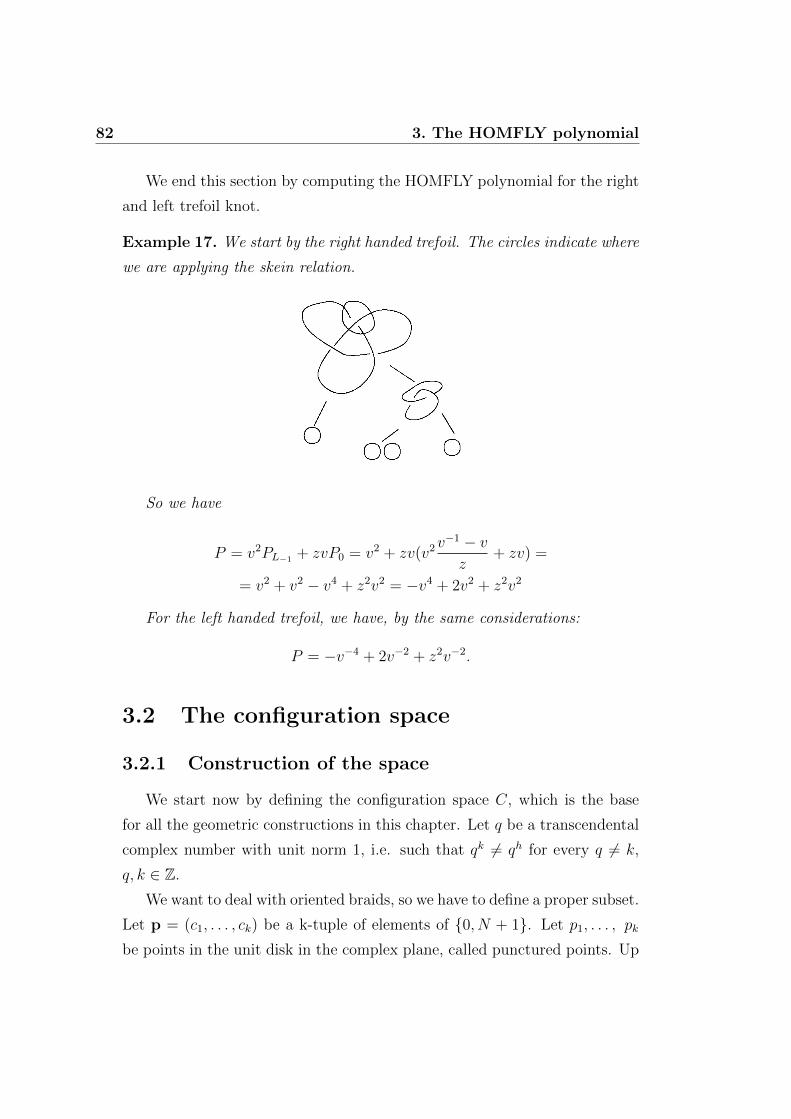
82 3. The HOMFLY polynomial
We end this section by computing the HOMFLY polynomial for the right
and left trefoil knot.
Example 17. We start by the right handed trefoil. The circles indicate where
we are applying the skein relation.
So we have
P = v2PL−1 + zvP0 = v2 + zv(v2v−1 − vz
+ zv) =
= v2 + v2 − v4 + z2v2 = −v4 + 2v2 + z2v2
For the left handed trefoil, we have, by the same considerations:
P = −v−4 + 2v−2 + z2v−2.
3.2 The configuration space
3.2.1 Construction of the space
We start now by defining the configuration space C, which is the base
for all the geometric constructions in this chapter. Let q be a transcendental
complex number with unit norm 1, i.e. such that qk 6= qh for every q 6= k,
q, k ∈ Z.
We want to deal with oriented braids, so we have to define a proper subset.
Let p = (c1, . . . , ck) be a k-tuple of elements of 0, N + 1. Let p1, . . . , pk
be points in the unit disk in the complex plane, called punctured points. Up
3.2 The configuration space 83
to diffeomorphism, we can choose the puncture points as lying on the real
line. To each point pi we can associate the number ci, called the colour of the
puncture point. The disk D with coloured puncture points is denoted as Dp.
Now, braids preserving the colours of the puncture points form a subgroup
of the braid group Bk, called the mixed braid group Bp.
Now, suppose m = (c′1, . . . , c′m), c′i ∈ 1, 2, . . . , N. We define a space C
as the set of m-tuples (x1, x2, . . . , xm), xi ∈ D, such that:
• if 1 ≤ i < j ≤ m and |c′i − c′j| ≤ 1, ⇒ xi 6= xj
• if 1 ≤ i ≤ m, 1 ≤ j ≤ k and |c′i − cj| = 1, ⇒ xi 6= pj
We can consider the subgroup of permutations W ⊂ Sm such that c′i =
c′w(i) for all i = 1, . . . ,m. W induces an action on C. We call Cm(Dp) the
quotient of C by this action.
The m-tuple (x1, . . . , xm) can be seen as a configuration of m points in D,
which we call mobile points. Every mobile point has colour assigned by the
array m. The first condition implies that two mobile points can coincide if
and only if their colours differ by at least two. The second condition implies
the same for a mobile point and a punctured point.
We have defined the configuration space, so the next step will be studying
its fundamental group. It is natural to try to represent its elements by using
braids. We can take the set p + m as
p + m = (c1, . . . , ck, c′1, . . . , c
′m)
So it is well defined the braid group Bp+m. Let G be the subgroup of those
mixed braids whose first k strands are straight. Now, if a pair of strands is
such that the colours differ by at least two, we can change the over/under
information of the crossing. Then the group π1(C) is the group obtained by
quotienting G by this relations.
We have defined the configuration space in a very general fashion, but in
the following we will focus on a particular case. We take p as the 2n-tuple
p = (0, N + 1, 0, N + 1, . . . , 0, N + 1)
84 3. The HOMFLY polynomial
In this way, the braid β we want to study is just an element in Bp, where
we take the strands whose colour is 0 as oriented downwards and the strands
whose colour is N + 1 as oriented upwards. Now, every knot or link can be
reconstructed from the plat closure of such a braid β, where the plat closure
β is the knot or link obtained by joining adjacent pairs of nodes at the top
and at the bottom of β. A proof of this statement can be found in [5].
Let m = Nn and m be the m-tuple
m = (1, 2, . . . , N, 1, 2, . . . , N, . . . , 1, 2, . . . , N)
We denote the configuration space Cm(Dp) as C. Now, we take an ho-
momorphism ρm : π1(C) → ±qk|k ∈ Z. We associate at every positive
crossing of a representation of g ∈ π1(C) as a braid group
• −q−1 if the two strands have the same colour
• q1/2 if the two strands have colours differing by one
• 1 otherwise
Let ρm(g) be the product of all the terms associated to the crossings of
a braid diagram. If we want it to be invariant by the second Reidemeister
move, it is straightforward to define a negative crossing as the reciprocal of
the analogous positive crossing. Also, the third condition implies that this is
well defined. For the definition of the space, the number of crossing whose
strand colours differ by 1 is even, so the exponent of q is effectively an integer.
Now, we want to define a homomorphism ρp : Bp → ±qk/2|k ∈ Z. As
earlier, we associate to every positive crossing of a braid representation of g
• qN/2 if the two strands have the same colour
• q−(N+1)/2 otherwise
As before, to every negative crossing we associate the reciprocal term
associated to the analogous positive crossing and we define ρp(g) as the
product of all the terms associated to the crossings.
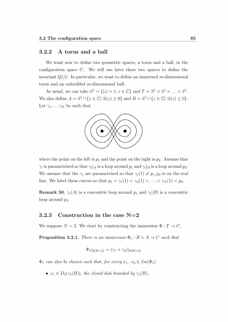
3.2 The configuration space 85
3.2.2 A torus and a ball
We want now to define two geometric spaces, a torus and a ball, in the
configuration space C. We will use later these two spaces to define the
invariant Q(β). In particular, we want to define an immersed m-dimensional
torus and an embedded m-dimensional ball.
As usual, we can take S1 = |z| = 1, z ∈ C and T = S1 × S1 × . . .× S1.
We also define A = S1∩z ∈ C| =(z) ≥ 0 and B = S1∩z ∈ C| =(z) ≤ 0.Let γ1, . . . γN be such that
where the point on the left is p1 and the point on the right is p2. Assume that
γi is parametrised so that γi|A is a loop around p1 and γi|B is a loop around p2.
We assume that the γi are parametrised so that γi(1) 6= p1, p2 is on the real
line. We label these curves so that p1 < γ1(1) < γ2(1) < . . . < γN(1) < p2.
Remark 50. γi(A) is a concentric loop around p1 and γi(B) is a concentric
loop around p2.
3.2.3 Construction in the case N=2
We suppose N = 2. We start by constructing the immersion Φ : T → C.
Proposition 3.2.1. There is an immersion Φ1 : B × A→ C such that
Φ1|∂(B×A) = (γ1 × γ2)|∂(B×A)
Φ1 can also be chosen such that, for every x1, x2 ∈ Im(Φ1)
• x1 ∈ D2(γ1(B)), the closed disk bounded by γ1(B),
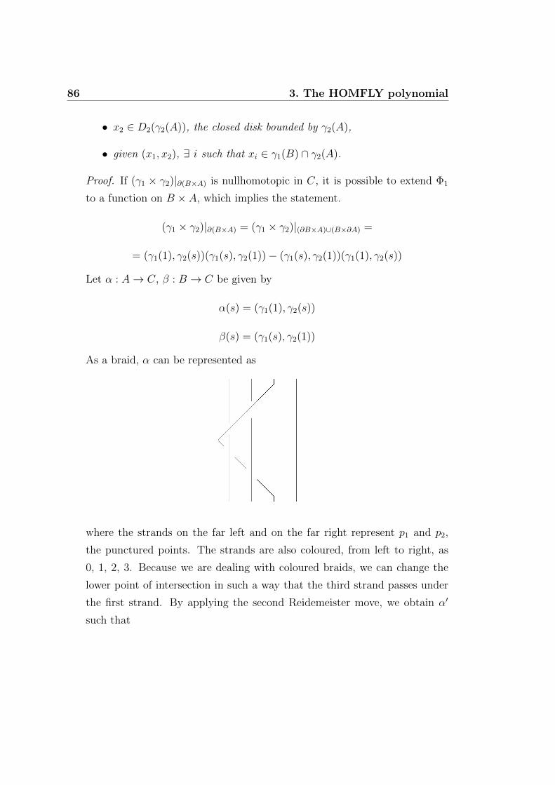
86 3. The HOMFLY polynomial
• x2 ∈ D2(γ2(A)), the closed disk bounded by γ2(A),
• given (x1, x2), ∃ i such that xi ∈ γ1(B) ∩ γ2(A).
Proof. If (γ1 × γ2)|∂(B×A) is nullhomotopic in C, it is possible to extend Φ1
to a function on B × A, which implies the statement.
(γ1 × γ2)|∂(B×A) = (γ1 × γ2)|(∂B×A)∪(B×∂A) =
= (γ1(1), γ2(s))(γ1(s), γ2(1))− (γ1(s), γ2(1))(γ1(1), γ2(s))
Let α : A→ C, β : B → C be given by
α(s) = (γ1(1), γ2(s))
β(s) = (γ1(s), γ2(1))
As a braid, α can be represented as
where the strands on the far left and on the far right represent p1 and p2,
the punctured points. The strands are also coloured, from left to right, as
0, 1, 2, 3. Because we are dealing with coloured braids, we can change the
lower point of intersection in such a way that the third strand passes under
the first strand. By applying the second Reidemeister move, we obtain α′
such that
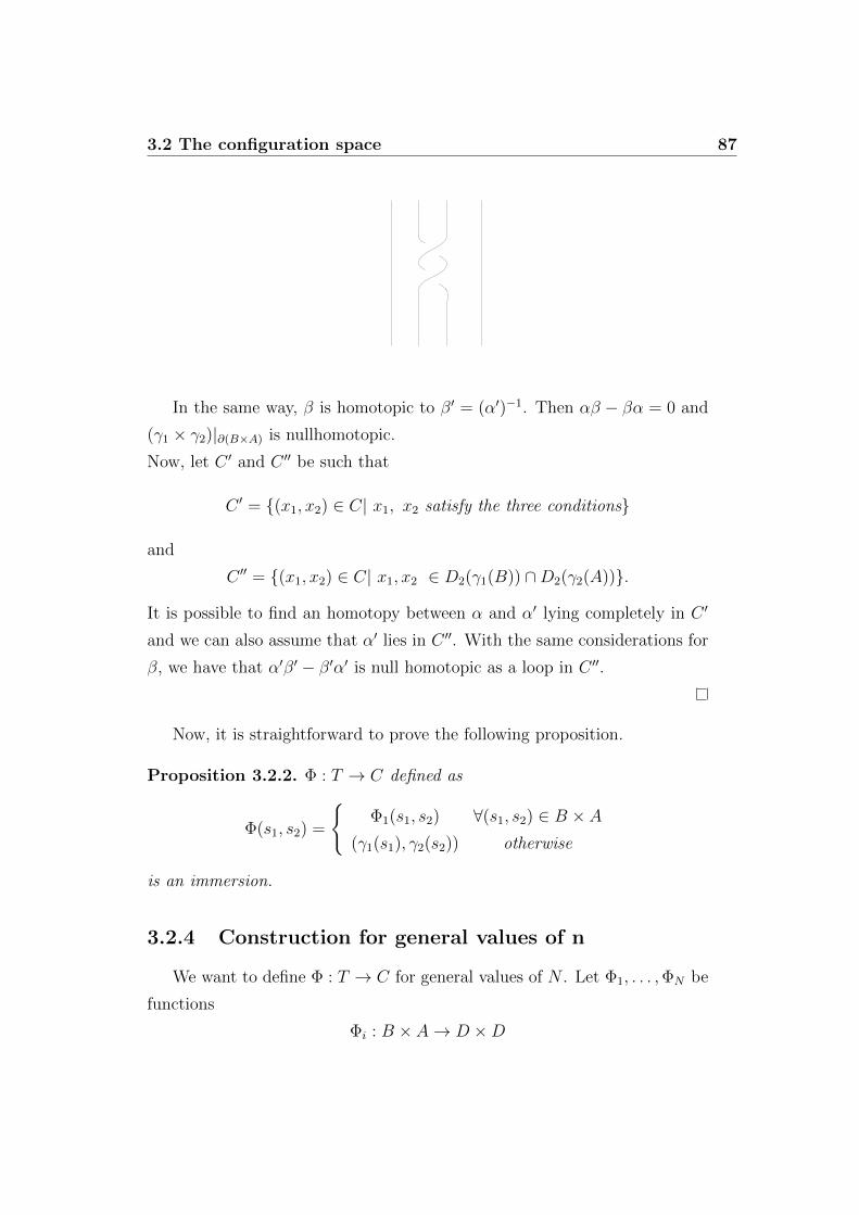
3.2 The configuration space 87
In the same way, β is homotopic to β′ = (α′)−1. Then αβ − βα = 0 and
(γ1 × γ2)|∂(B×A) is nullhomotopic.
Now, let C ′ and C ′′ be such that
C ′ = (x1, x2) ∈ C| x1, x2 satisfy the three conditions
and
C ′′ = (x1, x2) ∈ C| x1, x2 ∈ D2(γ1(B)) ∩D2(γ2(A)).
It is possible to find an homotopy between α and α′ lying completely in C ′
and we can also assume that α′ lies in C ′′. With the same considerations for
β, we have that α′β′ − β′α′ is null homotopic as a loop in C ′′.
Now, it is straightforward to prove the following proposition.
Proposition 3.2.2. Φ : T → C defined as
Φ(s1, s2) =
Φ1(s1, s2) ∀(s1, s2) ∈ B × A
(γ1(s1), γ2(s2)) otherwise
is an immersion.
3.2.4 Construction for general values of n
We want to define Φ : T → C for general values of N . Let Φ1, . . . ,ΦN be
functions
Φi : B × A→ D ×D

88 3. The HOMFLY polynomial
such that
Φi|∂(B×A) = (γi × γi+1)|∂(B×A)
and such that for all (xi, xi+1) ∈ Im(Φi)
• xi 6= xi+1
• xi ∈ D2(γi(B))
• xi+1 ∈ D2(γi+1(A))
• at least one between xi and xi+1 lies in D2(γi(B)) ∩D2(γi+1(A))
Now suppose (s1, . . . , sN) ∈ T . We let xi, i = 1, . . . , N be such that
• if si−1, si ∈ A then xi = γi(si)
• if si ∈ A and si−1 ∈ B then xi is the second coordinate of Φi−1(si−1, si)
• if si, si+1 ∈ B then xi = γi(si)
• if si ∈ B and si+1 ∈ A then xi is the first coordinate of Φi(si, si+1)
By convention, s0 ∈ A−B and sN ∈ B − A. Φ(s1, . . . , sn) = (x1, . . . , xn).
Proposition 3.2.3. Φ : T → C, defined as Φ(s1, . . . , sn) = (x1, . . . , xn), is
well defined.
Proof. If at least two of the conditions apply in the definition of xi, then they
all give xi = γi(si).
Since either x1 = γ1(s1) or x1 is the first coordinate of Φ(s1, s2), x1 6= p1
and similarly xN 6= p2.
We now check that xi 6= xi+1, ∀i = 1, . . . , N − 1.
We can suppose si ∈ A. Then for the first two conditions, xi should lie
in D2(γ1(A)) and xi+1 should not, thus xi 6= xi+1. The same if xi+1 ∈ B. If
si ∈ B and si+1 ∈ A, Φ(si, si+1) = (xi, xi+1), so xi 6= xi+1.
3.2 The configuration space 89
Proposition 3.2.4.
ρm Φ#(π1(T )) = 1
Proof. The group π(T ) = Z × Z × . . . × Z is generated by gi : S1 → T ,
i = 1, . . . , N , such that
gi(s) = (γ1(1), . . . , γi−1(1), γi(s), γi+1(1), . . . , γN(1))
The loop gi can be represented as a mixed braid with N +2 strands, with
every braid straight except the strand with colour i, describing a figure of
eight. We have two positive crossings involving a pair of strands with colours
i and i−1 and two negative crossings involving a pair of strands with colours
i and i+ 1. By definition of ρm, ρm(gi) = 1. Every g ∈ π1(T ) is combination
of elements gi, so ρm being a homomorphism, ρm(g) = 1.
Let X be X = D2(γ1(B))∩D2(γN(A)), CX = (x1, . . . , xN) ∈ C| ∃i, xi ∈X and TX = (s1, . . . , sN ∈ T | ∃i, si ∈ B and si+1 ∈ A). So Φ(TX) ⊂ CX
and Φ(T −TX) is a disjoint union of N + 1 embedded N -balls. If X is small,
it is possible to ignore Φ(TX) and just consider Φ(T − TX).
We have defined T as an oriented N -dimensional sub-manifold of C. We
want now to see that it is a pointed space, with a canonical choice for the
basepoint t. We start by N points t1, . . . , tN in the disk such that
• ti ∈ γi(B)
• =(ti) < 0
• γN(1) < <(t1) < <(t2) < . . . < <(tN) < p2
Then t = (t1, . . . , tN) is the canonical basepoint of T .
We want now to define a basepoint for C. For every i = 1, . . . , N , τi :
I → D is a vertical edge, τi(0) lying in the lower half of ∂D and τi(1) = ti.
x = τ(0) is the canonical basepoint for C and τ is a path between the two
basepoints
90 3. The HOMFLY polynomial
We now define an embedded ball in C. We start by the open N - ball
S = (s1, . . . , sN) ∈ RN | 0 < s1 < . . . < sN < 1. We parametrise the edge
from p1 to p2 by γ : I → D. We can define an embedding ψ : S → C by
ψ(s1, . . . , sN) = (γ(s1), . . . , γ(sN))
We want now to define a canonical basepoint for S. Let ηi : I → D be a
vertical edge from xi to a point in γ. η : I → C is the map
η(s) = (η1(s), . . . , ηN(s))
such that η(0) = x. We take the basepoint of S as s = η(1), and η becomes
a path from the basepoint x of C to the basepoint s of S.
We have defined S and T in the case C1 = C1,...,N(D0,N+1). We can define
an embedding∐
nC1 → C by gluing together n copies of D0,N+1. By taking
n copies of the immersed torus and of the embedded ball, we obtain the
general construction.
3.3 The invariant on braids
3.3.1 Definition
Now we define the invariant for a braid β by using the two spaces T and
S.
Remark 51. β is a diffeomorphism from D to itself, β(p1, . . . , p2n) =
p1, . . . , p2n and is such that it preserves the colours of the punctured points.
β induces an application from C to C, that we will also call β.
By construction, C is a 2m-dimensional manifold, while S and T are two
immersed m-manifolds. We can assume, up to isotopy, that they intersect
transversely at a finite number of points y1, . . . , yk. To each intersection
point yi we associate the sign at the intersection, εyi . We consider the path
3.4 A homological definition 91
ξy = (β τ)(γ1)(γ2)(η), where γ1 is a path in β(T ), γ1(0) = β(t), γ1(1) = y
and γ2 is a path in S, γ2(0) = y, γ2(1) = s. So we have:
< S, β(T ) >=∑
y∈S∩β(T )
εyρm(ξy)
It is very hard to compute directly this intersection. It is also necessary
to show that this definition is well defined, independent from the choices of
paths. This is why we are going to search an interpretation of this intersection
using algebraic topology.
3.4 A homological definition
Let L be the flat complex line bundle over C with monodromy given by
ρm. If we take (C, τd), where τd is the discrete topology, we can think of L
as a covering space of C, with every fibre given by C.
We denote by Hm(C;L) the m-dimensional homology of C with local
coefficients. We denote by H lfm (C;L) the m-dimensional locally finite homol-
ogy of C with local coefficients. In the following, we will write Hm(C) for
Hm(C;L). See the appendix A for the two definitions.
Theorem 3.4.1. Hm(C) and H lfm (C, ∂C) are isomorphic.
Proof. A proof can be found in [22].
Theorem 3.4.2. Hm(C) and Hom(Hm(C),C) are conjugate-isomorphic.
Proof. The theorem is an easy consequence of the universal coefficients the-
orem. A prove can be found in [14].
Corollary 3.4.3. H lfm (C, ∂C) and Hom(Hm(C),C) are conjugate isomor-
phic. Also, there is a sesquilinear pairing:
< ·, · >: H lfm (C, ∂C)×Hm(C)→ C
Remark 52. β induces an automorphism β# : π1(C) → π1(C) such that
ρm β# = ρm.
92 3. The HOMFLY polynomial
By remark 52, β lifts to an action on L, so there are induced actions on
Hm(C), Hm(C, ∂C) and H lfm (C).
We can identify the fibre over a point x with C. We have two lifts T and
S of the torus T and the ball S, leading to the following proposition.
Proposition 3.4.4. < S, β(T ) > is the sesquilinear pairing of S ∈ H lfm (C, ∂C)
and β(T ) ∈ Hm(C). It has the following proprieties:
• < S, β(T ) >=∑
y∈S∩β(T ) εyρm(ξy)
• it is invariant under the action of Bp
• if v1, v2 ∈ Hm(C), v′1, v′2 ∈ H lf
m (C, ∂C) are their images, then
< v′1, v2 >= (−1)m< v′2, v′1 >
Proof. The existence of the pairing is given by previous considerations. The
proprieties are proven in every book of algebraic topology, for example [14]
or [7].
Definition 59.
Q(β) =ρp(β)
[N + 1]qm/2< S, β(T ) >
where [N + 1], the quantum integer corresponding to N + 1, is
[N + 1] =q(N+1)/2 − q−(N+1)/2
q1/2 − q−1/2
3.4.1 Barcodes
Definition 60. Let CR be CR = (x1, . . . , xn) ∈ C| <(xi) = xi, ∀i =
1, . . . N.
Lemma 3.4.5. The map H lfm (CR) → H lf
m (C) induced by inclusion is an
isomorphism.
Proof. A proof can be found in [3].
3.4 A homological definition 93
Definition 61. A code sequence is a permutation of the sequence p + m
containing p as a subsequence.
Let S ′ be a connected component of CR and let y be y = (y1, . . . , ym) ∈ S ′,yi 6= yj ∀i, j, yi 6= pj ∀i, j. We call c = (c1, . . . , cm+n) a sequence of colours
of mobile points and puncture points, reading from right to left on the real
line. By definition, c is a code, representing S ′.
We want now to see some conditions about the code sequence. If there
is i ∈ 1, . . . N such that |ci − ci+1| ≥ 2, then it is possible to exchange ci
and ci+1 without altering the connected component of CR. This follows from
the construction of C and the conditions about the movements of the mobile
points.
Definition 62. The code sequences are equivalent if they are related by
exchanges between ci and ci+1, where at least one among ci and ci+1 lies in
1, . . . , N and |ci+1 − ci| ≥ 2.
If a code sequence c is equivalent to a code sequence whose first or last
entry lies in 1, . . . N, then c is said to be trivial.
Remark 53. The equivalence classes of code sequences are in bijective cor-
respondence with the connected components of CR.
Proposition 3.4.6. Let c be a sequence and S ′ the associated connected
component of CR.
If c is trivial, S ′ is homeomorphic to the upper half space in Rm.
If c is not trivial, S ′ is homeomorphic to an open m-ball.
Proof. If c is trivial, then S ′ contains a point (y1, . . . , ym) such that y1 or ym
lies in ∂D.
If c is not trivial, every point in S ′ is a configuration of points between
p1 and p2n.
Proposition 3.4.7. Let Rm+ be the upper half space in Rm. Then
H lfm (Rm
+ ) = 0,
H lfm (Rm) = C.
94 3. The HOMFLY polynomial
Proof. A proof can be found in [14] or in [6].
3.4.2 Basis for the homology
Let us choose a non zero element in H lfm (S ′) associated to a given non-
trivial code sequence c. By lemma 3.4.5 and proposition 3.4.6 this is a basis
for H lfm (C), for which we should choose an orientation and a lift to L.
Let < ·, · > be the non-degenerate sesquilinear pairing
< ·, · >′: H lfm (C)×Hm(C, ∂C)→ C
Then we can define a basis for Hm(C, ∂C) by dualising the basis for H lfm
with respect to the pairing. We will now give a geometric construction of the
homology classes.
Let D2 be a disk in the complex plane and let E1, . . . , Em be properly
embedded vertical edges in D2, Ei ∩ Ej = ∅, ∀i 6= j and pi /∈ Ej ∀i, j. Now,
the product of these edges is an embedded closed m-ball in C. We will call
this ball Z. We can take the code sequence c = (c1, . . . , cm+n), given by the
sequence of colours of the punctured points or of vertical edges.
It is possible to lift every Z to L, representing an element in Hm(C, ∂C).
Definition 63. Z denotes both the embedded m-ball and an element in
Hm(C, ∂C). Z will be called the barcode corresponding to the code sequence
c.
Remark 54. Two equivalent code sequences give rise to the same barcode
in Hm(C, ∂C), up to choices of lifts to L.
Proposition 3.4.8. If c is a trivial code, then any barcode corresponding to
c is zero.
A basis for Hm(C, ∂C) is given by non-zero barcodes corresponding to
each non-trivial code sequence c.
3.4 A homological definition 95
Proof. Let S ′ be a component of CR and Z be a barcode. If S ′ and Z
correspond to the same non-trivial code sequence c, then S ′ ∩ Z = point,so, up to choices of orientations and lifts, < S ′, Z >= 1. Instead, if S ′ and
Z correspond to different code sequences, then S ∩Z = ∅ and < S ′, Z >= 0.
Thus the basis is well defined as the dual of the basis of H lfm (C).
3.4.3 The image of T
In this paragraph we want to compute T in H lfm (C) and in Hm(C, ∂C).
To start, we suppose n = 1.
Remark 55. If n = 1, the only non trivial sequence is (0, 1, . . . , N + 1). We
will call simply as Z its barcode, product of the edges 1, . . . , N in order and
we choose a lift to L such that it contains the point 1 in the fibre over the
basepoint x.
Proposition 3.4.9. The image of T ∈ H lfm (C) is (q − 1)mS.
Proof. Having assumed n = 1, by remark 55 there is only one non-trivialcode
sequence, so H lfm (C) = C and T = λS.
We have defined T by figures of eight γ1, . . . , γN and Z by edges E1, . . . , EN .
By construction, γi intersects Ei at two points, y+i and y−i . So, T and Z in-
tersect at the 2N points
(y±1 , . . . , y±N)
Every such point contributes a monomial ±qk to < T,Z >.
Let t be t = (y−1 , . . . , y−N) such that the orientation of the intersection at
y−i is positive. Thus t contributes 1 to < T,Z >′.
Let us compute by induction the contributions of the other points. Let y,
y′ be points differing at the mobile point of colour i. We can assume y taking
the value y−i and y′ taking the value y+i . We define a loop η, η(0) = η(1) = y′,
such that it follows a path in T from y to y′ and then back to y′ along a path
in Z. A braid representing it is such that all the strands are straight, with the
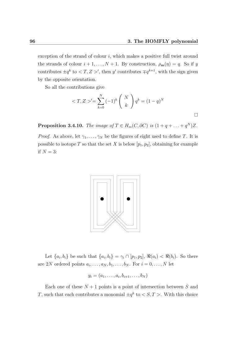
96 3. The HOMFLY polynomial
exception of the strand of colour i, which makes a positive full twist around
the strands of colour i + 1, . . . , N + 1. By construction, ρm(η) = q. So if y
contributes ±qk to < T,Z >′, then y′ contributes ∓qk+1, with the sign given
by the opposite orientation.
So all the contributions give
< T,Z >′=N∑k=0
(−1)k
(N
k
)qk = (1− q)N
Proposition 3.4.10. The image of T ∈ Hm(C, ∂C) is (1 + q + . . .+ qN)Z.
Proof. As above, let γ1, . . . , γN be the figures of eight used to define T . It is
possible to isotope T so that the set X is below [p1, p2], obtaining for example
if N = 3:
Let ai, bi be such that ai, bi = γi ∩ [p1, p2], <(ai) < <(bi). So there
are 2N ordered points ai, . . . , aN , b1, . . . , bN . For i = 0, . . . , N let
yi = (a1, . . . , ai, bi+1, . . . , bN)
Each one of these N + 1 points is a point of intersection between S and
T , such that each contributes a monomial ±qk to < S, T >. With this choice
3.4 A homological definition 97
of orientations, the signs of the intersections of S and T at yi are positive
for every i. Also, yN contributes 1 to < S, T >. As in the previous proof,
we assume that η is a loop, η(0) = η(1) = y, following a path in T from yi
to yi−1, and then a patch in S from yi−1 to yi. Again, if we see this loop as
a braid, all the strands are straight, except the strand of colour i, acting as
in the last proof. So again ρm(η) = q. So, if yi contributes qk, yi contributes
qk−1. Then
< S, T >= 1 + q + . . .+ qN
and comparing with < S,Z >= 1 we obtain the claim.
Proposition 3.4.11. The image of T ∈ H lfm (C) is (q − 1)mS.
Proof. By construction of T , the general case is a trivial consequence of the
case n = 1.
3.4.4 Partial bar codes
We had defined S as the product of N -balls S1, . . . , SN . Being Z the
non-trivial barcode for n = 1, let Zi be
Zi = S1 × . . .× Si−1 × Z × Si+1 × . . .× SN
with basepoint s lying in Zi. So the path η determines a lift of Zi to L,
giving an element in H lfm (C, ∂C).
Proposition 3.4.12. (q − 1)NS = (1 + q + . . .+ qN)Zi ∈ H lfm (C, ∂C).
Proof. For the case n = 1, by previous computation we have
T = (1 + q + . . .+ qN)Z1, T = (q − 1)NS
.
We assume now n > 1. We start by stretching T and using excision to
obtain a disjoint union of bar codes, where one is Zi and the others are trivial
98 3. The HOMFLY polynomial
code sequences. Such a barcode is 0 ∈ H lfm (C, ∂C), since one of the vertical
edges can be slid to the boundary of the disk, ending the construction for
n = 1.
We want now to do something similar for the case n > 1. Let m′ be
m′ = (1, 2, . . . , N, j), j = 1, . . . , N . Let C ′ be the configuration space
C ′ = Cm′(D(0,N+1))
Let S ′ be the product of the N -ball in C(1,...,N)(D(0,N+1)) and a circle of
colour j around [p1, p2]. S ′ is a (N + 1)-dimensional sub-manifold of C ′.
For homotopy equivalence, π1(S ′) = Z, generated by g. The loop g can
be represented by a braid with straight strands, with the exception of the
strand of colour i making a positive full twist around the other strands, so
that ρm(g) = 1. So it is possible to lift S ′ to L, representing an element in
H lfm (C) also called S ′.
We want now to show that S ′ = 0 ∈ H lfm (C). Assuming N = 1, S ′ is
simply the product of an edge γ between the two puncture points and a
circle δ around γ. We call Z the barcode corresponding to the only non-
trivial sequence (0,1,1,2). Let E and E ′ be the two vertical edges of colour 1
between the two punctured points, E being to the right of E. So we can see
Z as a closed 2-ball, being the product of E and E ′.
We have E ∩ (γ ∪ δ) = a1, a2, a3, E ′ ∩ (γ ∪ δ) = b1, b2, b3. We then
have 4 points of intersection between S ′ and Z,
• y1 = (a2, b1)
• y2 = (a2, b3)
• y3 = (a1, b2)
• y4 = (a3, b2)
We are supposed to have chosen y1 such that its contribution is 1. Now,
for i = 2, 3, , 4, ξi is a loop following a path in Z from y1 to yi and a path in
S ′ from yi to y1. So we obtain
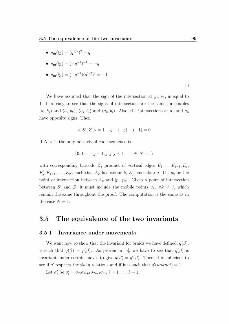
3.5 The equivalence of the two invariants 99
• ρm(ξ2) = (q1/2)2 = q
• ρm(ξ3) = (−q−1)−1 = −q
• ρm(ξ4) = (−q−1)(q1/2)2 = −1
We have assumed that the sign of the intersection at y1, ε1, is equal to
1. It is easy to see that the signs of intersection are the same for couples
(ai, bj) and (ai, bk), (aj, bi) and (ak, bi). Also, the intersections at a1 and a3
have opposite signs. Then
< S ′, Z >′= 1− q − (−q) + (−1) = 0
If N > 1, the only non-trivial code sequence is
(0, 1, . . . , j − 1, j, j, j + 1, . . . , N,N + 1)
with corresponding barcode Z, product of vertical edges E1 . . . , Ej−1, Ej,
E ′j, Ej+1, . . . , EN , such that Ek has colour k, E ′j has colour j. Let yk be the
point of intersection between Ek and [p1, p2]. Given a point of intersection
between S ′ and Z, it must include the mobile points yk, ∀k 6= j, which
remain the same throughout the proof. The computation is the same as in
the case N = 1.
3.5 The equivalence of the two invariants
3.5.1 Invariance under movements
We want now to show that the invariant for braids we have defined, q(β),
is such that q(β) = p(β). As proven in [5], we have to see that q(β) is
invariant under certain moves to give q(β) = q′(β). Then, it is sufficient to
see if q′ respects the skein relations and if it is such that q′(unknot) = 1.
Let σ′i be σ′i = σ2iσ2i+1σ2i−1σ2i, i = 1, . . . , b− 1.
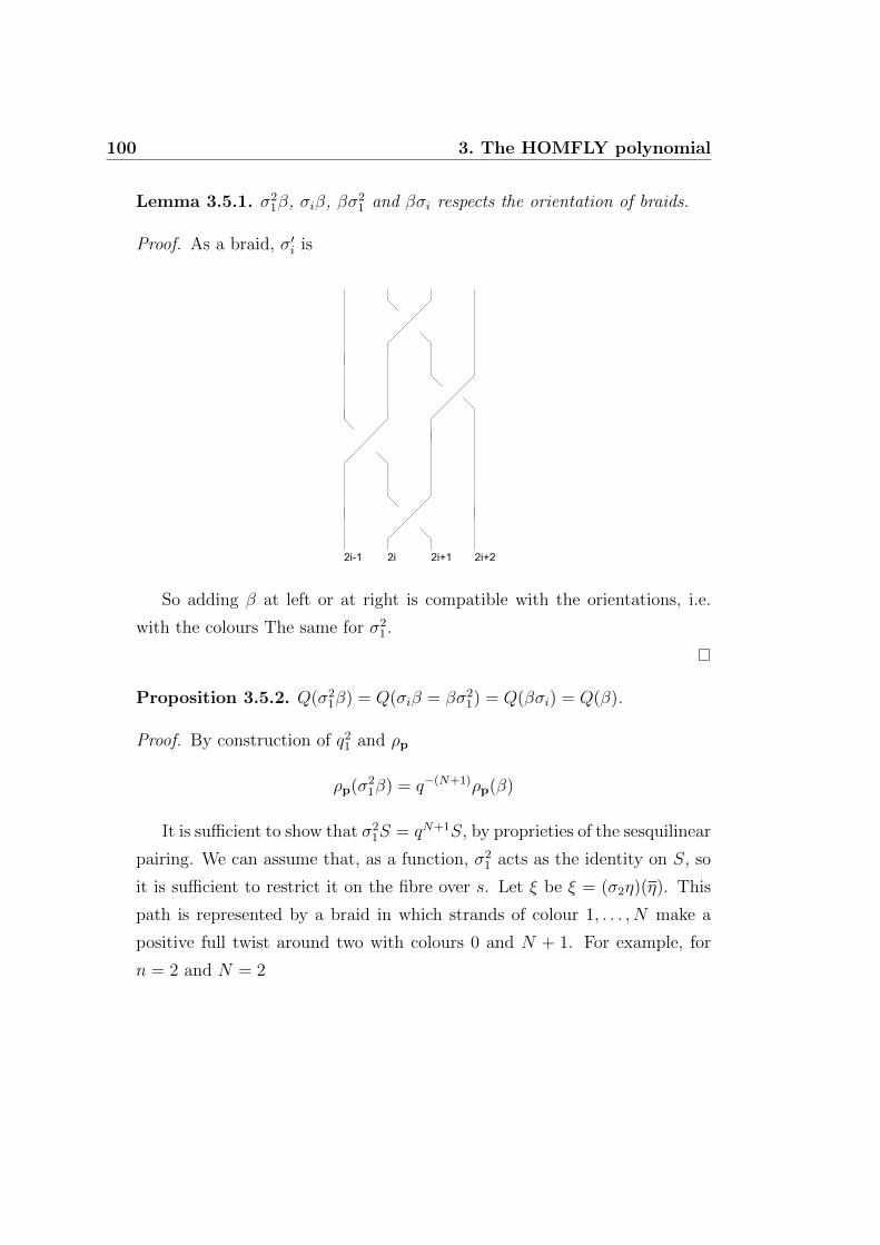
100 3. The HOMFLY polynomial
Lemma 3.5.1. σ21β, σiβ, βσ2
1 and βσi respects the orientation of braids.
Proof. As a braid, σ′i is
2i-1 2i 2i+1 2i+2
So adding β at left or at right is compatible with the orientations, i.e.
with the colours The same for σ21.
Proposition 3.5.2. Q(σ21β) = Q(σiβ = βσ2
1) = Q(βσi) = Q(β).
Proof. By construction of q21 and ρp
ρp(σ21β) = q−(N+1)ρp(β)
It is sufficient to show that σ21S = qN+1S, by proprieties of the sesquilinear
pairing. We can assume that, as a function, σ21 acts as the identity on S, so
it is sufficient to restrict it on the fibre over s. Let ξ be ξ = (σ2η)(η). This
path is represented by a braid in which strands of colour 1, . . . , N make a
positive full twist around two with colours 0 and N + 1. For example, for
n = 2 and N = 2
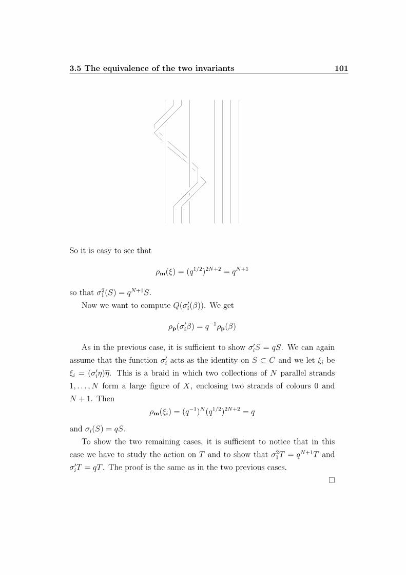
3.5 The equivalence of the two invariants 101
So it is easy to see that
ρm(ξ) = (q1/2)2N+2 = qN+1
so that σ21(S) = qN+1S.
Now we want to compute Q(σ′i(β)). We get
ρp(σ′iβ) = q−1ρp(β)
As in the previous case, it is sufficient to show σ′iS = qS. We can again
assume that the function σ′i acts as the identity on S ⊂ C and we let ξi be
ξi = (σ′iη)η. This is a braid in which two collections of N parallel strands
1, . . . , N form a large figure of X, enclosing two strands of colours 0 and
N + 1. Then
ρm(ξi) = (q−1)N(q1/2)2N+2 = q
and σi(S) = qS.
To show the two remaining cases, it is sufficient to notice that in this
case we have to study the action on T and to show that σ21T = qN+1T and
σ′iT = qT . The proof is the same as in the two previous cases.
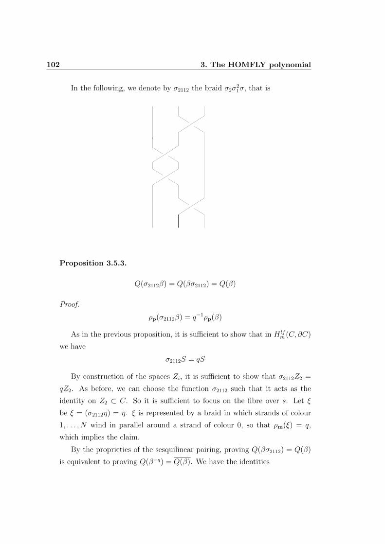
102 3. The HOMFLY polynomial
In the following, we denote by σ2112 the braid σ2σ21σ, that is
Proposition 3.5.3.
Q(σ2112β) = Q(βσ2112) = Q(β)
Proof.
ρp(σ2112β) = q−1ρp(β)
As in the previous proposition, it is sufficient to show that in H lfm (C, ∂C)
we have
σ2112S = qS
By construction of the spaces Zi, it is sufficient to show that σ2112Z2 =
qZ2. As before, we can choose the function σ2112 such that it acts as the
identity on Z2 ⊂ C. So it is sufficient to focus on the fibre over s. Let ξ
be ξ = (σ2112η) = η. ξ is represented by a braid in which strands of colour
1, . . . , N wind in parallel around a strand of colour 0, so that ρm(ξ) = q,
which implies the claim.
By the proprieties of the sesquilinear pairing, proving Q(βσ2112) = Q(β)
is equivalent to proving Q(β−q) = Q(β). We have the identities
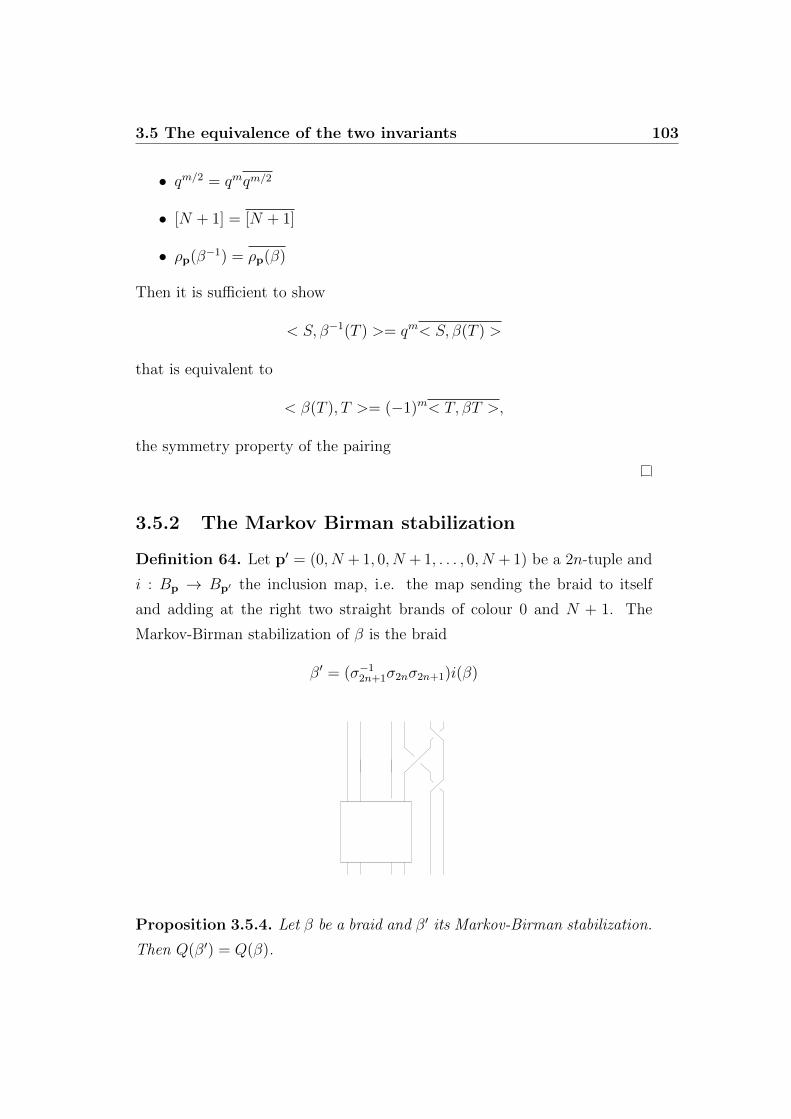
3.5 The equivalence of the two invariants 103
• qm/2 = qmqm/2
• [N + 1] = [N + 1]
• ρp(β−1) = ρp(β)
Then it is sufficient to show
< S, β−1(T ) >= qm< S, β(T ) >
that is equivalent to
< β(T ), T >= (−1)m< T, βT >,
the symmetry property of the pairing
3.5.2 The Markov Birman stabilization
Definition 64. Let p′ = (0, N + 1, 0, N + 1, . . . , 0, N + 1) be a 2n-tuple and
i : Bp → Bp′ the inclusion map, i.e. the map sending the braid to itself
and adding at the right two straight brands of colour 0 and N + 1. The
Markov-Birman stabilization of β is the braid
β′ = (σ−12n+1σ2nσ2n+1)i(β)
Proposition 3.5.4. Let β be a braid and β′ its Markov-Birman stabilization.
Then Q(β′) = Q(β).
104 3. The HOMFLY polynomial
Proof. Let m′ be the m + N -tuple (1, . . . , N, 1, . . . , N, . . . , 1, . . . , N), D′ =
Dp′ , C′ = Cm′(D
′) and S ′ and T ′ the embedded m′-ball and the immersed
m′-torus in C ′. Then
< S ′, β′(T ′) >=< S, β(T ) >
by the identities
• ρp(β′) = qN/2ρp(β)
• qm′/2 = qN/2qm/2
Let now Zn ⊂ C and Z ′N ⊂ C ′ be defined by replacing the second to
rightmost N -ball of S ′ by a barcode. So we have
< Z ′n, β′(T ′) >=< Zn, β(T ) >
which is equivalent to
< σ(Z ′n), i(β)(T ′) >=< Zn, β(T ) >
with σ = σ−12n+1σ
−12n σ2n+1. It is sufficient to compute this intersection.
Let D3 be a disk with three punctured points. We imagine D3 as the set
of points in D′ to the right of a vertical line between p2n−1 and p2n. So we
can identify the three punctured points with p2n, p2n+1 and p2n+2. We can
define an embedding
Cm(D′ −D3)× C(1,...,N)(D3)→ C ′
Assuming that Zn lies in Cm(D′ −D3) and taking Sn+1 as the N -ball in
C(1,...,N)(D3), we get
Z ′n = Zn × Sn+1
Then
σ(Z ′n) = Zn × σ(Sn+1)
3.5 The equivalence of the two invariants 105
Now, let D2 be a disk with two punctured points. As above, we can
imagine it as the set of points in D′ to the right of a vertical line between
p2n and p2n+1, so that we can identify the two punctured points with p2n+1
and p2n+2. There is an embedding
Cm(D′ −D2)× C(1,...,N)(D2)→ C ′
Assuming that T lies in Cm(D′−D2) and letting TN+1 be theN -dimensional
torus in C(1,...,N)(D2), we get
T ′ = T × Tn+1
so that
i(β)(T ′) = β(T )× Tn+1
By the above computation, we obtain
< Z × σ(Sn+1), β(T )× Tn+1 >=< Z, β(T ) >
Any point of intersection between Z × σ(Sn+1) and β(T ) × Tn+1 lies in
the intersection of the two product spaces
Cm(D′ −D3)× C(1,...,N)(D2)
So it is sufficient to show that
< σ(Sn+1), Tn+1 >= 1
By restriction, we can see this intersection pairing as being between sub-
manifolds of C(1,...,N)(D3). We should now compute directly this pairing.
There is one point of intersection y between σ(Sn+1) and Tn+1. We can
assume the sign of this intersection to be positive. Now, both σ(Sn+1) and
Tn+1 have associated paths from a configuration of points on ∂D3 to y, paths
that are homotopic relative to endpoints, which completes the proof. For
example, in the case N = 1 we have
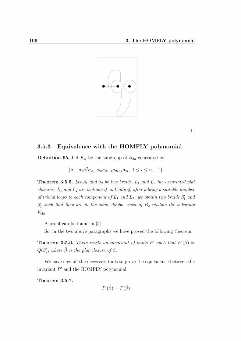
106 3. The HOMFLY polynomial
3.5.3 Equivalence with the HOMFLY polynomial
Definition 65. Let Kn be the subgroup of B2n generated by
σ1, σ2σ21σ2, σ2iσ2i−1σ2i+1σ2i, 1 ≤ i ≤ n− 1.
Theorem 3.5.5. Let β1 and β2 be two braids, L1 and L2 the associated plat
closures. L1 and L2 are isotopic if and only if, after adding a suitable number
of trivial loops to each component of L1 and L2, we obtain two braids β′1 and
β′2 such that they are in the some double coset of B2 modulo the subgroup
K2n.
A proof can be found in [5]
So, in the two above paragraphs we have proved the following theorem
Theorem 3.5.6. There exists an invariant of knots P ′ such that P ′(β) =
Q(β), where β is the plat closure of β.
We have now all the necessary tools to prove the equivalence between the
invariant P ′ and the HOMFLY polynomial.
Theorem 3.5.7.
P ′(β) = P (β)
3.5 The equivalence of the two invariants 107
Proof. It has been proven in [12] that there exists an unique polynomial P
such that
• P respects the skein relation,
• P (unknot) = 1.
Then it is sufficient to show that P ′ also respects the two conditions.
We begin by proving that P ′ respects the skein relation. Let β+ and β−
be
β+ = σ−12 σ1σ2β, β− = σ−1
2 σ−11 σ2β.
Up to isotopy, it is sufficient then to show
q(N+1)/2Q(β−)− q−(N+1)/2Q(β+) = (q1/2 − q−1/2)Q(β)
By definition
• ρp(β+) = qN/2ρp(β)
• ρp(β−) = q−N/2ρp(β)
So we should show
q1/2 < S, β−(T ) > −q−1/2 < S, β+(T ) >= (q1/2 − q−1/2) < S, β(T ) >
We can take, instead of S, the subspace Z2, so that we can restrict to
show
q1/2 < Z2, β−(T ) > −q−1/2 < Z2, β+(T ) >= (q1/2 − q−1/2) < Z2, β(T ) >
that is equivalent to
< σ−12 (σ1 − 1)(1 + qσ−1
1 )σ2(Z2), β(T ) >= 0
We will not compute the intersection pairing, but we will show that in
H lfm (C, ∂C) we have
σ−12 (σ1 − 1)(1 + qσ−1
1 )σ2(Z2) = 0
108 3. The HOMFLY polynomial
Let D3 be a three times punctured disk, which can be identified with
the set of points in D to the left of a vertical line between p3 and p4, such
that the three punctured points can be identified with p1, p2 and p3. Let C1 =
C(1...,N)(D3) and m2 be them−N -tuple m2 = (1, . . . , N, 1, . . . , N, . . . , 1, . . . , N)
and C2 = Cm2(D −D3). We consider the embedding
C1 × C2 → C.
Taking S1 as the N -ball in C1 and Z ′ as an (N −m)-manifold in C2 we
have
Z2 = S1 × Z ′.
σ1 and σ2 are such that they act as the identity on D − D3. Thus it is
sufficient to show that in H lfN (C1)
σ−12 (σ1 − 1)(1 + qσ−1
1 σ2)(S1) = 0
Let now D′3 be D′3 = σD3, a three times punctured disk with colours,
from left to right, 0, 0 and N + 1. Let C ′1 be C ′1 = C(1,...,N)(D′3) and S ′1 be
S ′1 = σ2S1. Then we have
(σ1 − 1)(1 + qσ−11 )(S ′1) = 0
in H lfN (C ′1).
It is easy to see that in this setting there are only two non-trivial se-
quences, (0, 1, 2, . . . , N + 1, 0) and (0, N + 1, N, . . . , 1, 0). Let Z be the bar-
code corresponding to the non-trivial code sequence (0, 1, 2, . . . , N+1, 0). So
S ′1 and Z do not intersect and < S ′1, Z >′= 0.
Instead, σ1(S ′1) and Z intersect at a single point, and so do σ−11 (S ′1) and
Z. The two intersection points are such that their signs are the same. We
assume that the two points of intersection coincide on y. Now, each of σ1(S ′1)
and σ−11 (S ′1) are associated to a path from y to x, paths that differ by the
direction the points of colours 1, . . . , N pass around the middle puncture
point, so that
< σ−11 (S ′1), Z ′ >′= q < σ1(S ′1), Z > .
3.5 The equivalence of the two invariants 109
By computation,
< (σ1 − 1)(1 + qσ−11 )(S ′1), Z >′= 0.
Let Z be the barcode corresponding to (0, N + 1, N, . . . , 1, 0) and let us
assume that σ1 acts as the identity on Z. So we have
< S ′1, Z >′=< σ−11 (S ′1), Z >′
and by computation
< (σ1 − 1)(1 + qσ−11 )(S ′1), Z >′= 0.
So we have proven that P ′ respects the skein relation. We now see that
P ′(unknot) = 1. Suppose n = 1 and β is the identity braid. We have proven
that
< S, T >= 1 + q + . . .+ qN
and so
Q(β) =1
[N + 1]qN/2(1 + q + . . .+ qN) = 1
So we have proven that P ′(β) = Q(β) = 1, which ends the proof.

110 3. The HOMFLY polynomial

Appendix A
Local Coefficients via Bundles
of Groups
Definition 66. Let E and X be two topological spaces and let p be a map
p : E → X such that each point of X admits a neighborhood U for which
there is a homeomorphism ϕU : p−1(U) → U × G taking each p−1(x) to
x × G by a group isomorphism. The map p is called a bundle of groups,
the subsets p−1(x) are called the fibers of p and E is said to be a bundle of
groups with fiber G.
Remark 56. If we take (G, τD), where τD is the discrete topology, p is a
covering space.
Let σi : ∆n → X be a singular n-simplex in X and let ni : ∆n → E be a
lifting of σi. We can then take finite sums∑m
i=1 niσi. Given two lifts ni and
mi of the same lift σi, we can define their sum as (ni+mi)(s) = ni(s)+mi(s),
which is still a lift of σi. So we have defined an abelian group Cn(X;E). We
want it to be a chain complex.
We can define a boundary homomorphism ∂ : Cn(X;E) → Cn−1(X;E)
by
∂(∑i
niσi) =∑i,j
(−1)jni|v0,...,vj ,...,vnσi|v0,...,vj ,...,vn
We can notice that the boundary is linear and it acts on σi as the
111

112 A. Local Coefficients via Bundles of Groups
usual boundary for singular homology. Then it is obvious that ∂2 = 0 and
(C∗(X;E), ∂) is a chain complex, whose homology groups are denoted as
H∗(X;E).
Let f : X → X ′ be a map. We want to find conditions for which it
induces a map in homology with local coefficients. Let p′ : E ′ → X ′ be a
bundle of groups. We define E as
E = (x, e′) ∈ X × E ′| f(x) = p′(e′)
and p : E → X as p(x, e′) = x. Let f : E → E ′ be f(x, e′) = e′. By
definition, the fiber p−1(x) is the set (x, e′) ∈ X × E| f(x) = p′(e′), so
that f is a bijection between p−1(x) and p′−1(f(x)) and p−1(x) has a group
structure.
By definition of bundle of groups, ϕ′ : (p′)−1(U ′)→ U ′ ×G is an isomor-
phism. Let U be U = f−1(U ′) and let ϕ be ϕ : p−1(U)→ U ×G, defined by
ϕ(x, e′) = (x, ϕ′2(e′)). So ϕ admits as inverse and then it is an isomorphism
on each fiber. The bundle of groups p is called the pullback of p′, or the
induced bundle.
Let us now define the cohomology groups. Let Φ be a function from the
set of singular n-simpleces to E, assigning to each σ ∈ ∆n a lift Φ(σ) ∈ E. Let
Cn(X;E) be the group of such functions. The definition of the coboundary
map δ : Cn(X;E) → Cn+1(X;E) is exactly as in singular cohomology, so
that δ2 = 0 and (Cn(X;E), δ) is a cochain complex. Let Hn(X;E) be the
cohomology of such a complex.
We now define the homology groups H lfn (X;G). Let σ : ∆n → X be a
singular simplex. We take the set C lfn of locally finite chains, which are formal
sums∑
σ gσσ, gσ ∈ G, such that every x ∈ X admits a neighborhood U such
that U meets the images of a finite number of σ with gσ 6= 0. The boundary
operator is obviously well defined, because if σ satisfies the condition, so
does its boundary. The homology H lf∗ (X;G) is the homology of this chain
complex.
Bibliography
[1] M. Artin, Algebra, Pearson Education, Boston, 2010.
[2] S. Bigelow, A homological definition of the jones polynomial, Geome-
try and Topology Monographs, 4 (2001), pp. 29–41).
[3] , Homological representations of the iwahori-hecke algebra, Proceed-
ings of the Casson Fest, Geom. Topol. Monogr., 7 (2004), pp. 493–507
(electronic).
[4] , A homological definition of the homfly polynomial,
arXiv:math/0608527v1, (2006).
[5] J. S. Birman, On the stable equivalence of plat representatons of knots
and links, Can. J. Math., XXVIII (1976), pp. 264–290.
[6] R. Bott and L. W. Tu, Differential forms in algebraic topology,
Springer, New York, 1982.
[7] G. Bradon, Topology and Geometry, Springer, New York, 1993.
[8] G. Burde and H. Zeischagl, Knots, De Gruyter Studies in Mathe-
matics, New York, 2003.
[9] R. Fox, Derivation in the free group ring., Ann. Of. Math,, (1953),
pp. 547–560.
[10] , The isomorphism problem., Ann. Of. Math,, (1954), pp. 196–210.
[11] , Subgroups., Ann. Of. Math, (1956), pp. 407–419.
113

114 BIBLIOGRAPHY
[12] P. Freyd, D. Yetter, J. Hoste, W. Lickorish, K. Millett,
and A. Ocneanu, A new polynomial invariant of knots and links, Bul-
letin of the American Mathematical Society, 12 (1985), pp. 239–246.
[13] V. L. Hansen, Braids and coverings: selected topics, Cambridge Uni-
versity Press, Cambridge, 1989.
[14] A. Hatcher, Algebraic Topology, Cambridge University Press, New
York, 2001.
[15] V. F. R. Jones, A polynomial invariant for knots via von neumann
algebra, Bulletin of the American Mathematical Society, 12 (1985),
pp. 103–111.
[16] C. Kassel and V. Turaev, Braid Groups, Spinger, New York, 2008.
[17] Lickorish, An introduction to knot theory, Springer, New York, 1964.
[18] R. Lyndon and P. Schupp, Combinatorial Group Theory, Springer,
New York, 1982.
[19] A. Malcev, On isomorphic matrix representations of infinite groups,
Rec. Math., (1940), pp. 405–422.
[20] A. Markov, Foundations of the algebraic theory of braids, (1945, jour-
nal = Trudy Math. Inst. Steklov 16), pp. 1–54.
[21] Murakami, Ohtsuki, and Yamada, Homfly polynomial via an in-
variant of colored planar graphs, Ens. Math., (1998), pp. 325–360.
[22] E. Spanier, Singular homology and cohomology with local coefficients
and duality for manifolds, Pacific Journal of Mathematics, 160 (1993).
[23] J. Stillwell, Classical topology and combinatorial group theory,
Springer-Verlag, New York, 1980.
[24] Turaev, Quantum Invariants of Knots and 3-Manifolds, De Gruyter,
Berlin, 1994.
BIBLIOGRAPHY 115
[25] , Faithful linear representation of the braid groups, Seminaire Bour-
baki, (2000).
[26] P. Vogel, Representation of links by braids: A new algorithm, Com-
mentarii Mathematici Helvetici, 65 (1990), pp. 104–113.