A one-dimensional tunable magnetic metamaterial - Optics InfoBase

A one-dimensional tunable magneticmetamaterial

S. Butz1, P. Jung1, L. V. Filippenko2,3, V. P. Koshelets2,3, andA. V. Ustinov1,3

1Physikalisches Institut, Karlsruhe Institute of Technology, 76131 Karlsruhe, Germany2Kotel’nikov Institute of Radio Engineering and Electronics (IREE RAS), Moscow 125009,

Russia3National University of Science and Technology MISIS, Moscow 119049, Russia

*[email protected]

Abstract: We present experimental data on a one-dimensional super-conducting metamaterial that is tunable over a broad frequency band. Thebasic building block of this magnetic thin-film medium is a single-junction(rf-) superconducting quantum interference device (SQUID). Due tothe nonlinear inductance of such an element, its resonance frequency istunable in situ by applying a dc magnetic field. We demonstrate that thisresults in tunable effective parameters of our metamaterial consisting of54 rf-SQUIDs. In order to obtain the effective magnetic permeability µr,efffrom the measured data, we employ a technique that uses only the complextransmission coefficient S21.

© 2013 Optical Society of America

OCIS codes: (160.3918), (310.2790), (310, 6628), (350.4010).

References and links1. M. C. Ricci, N. Orloff, and S. M. Anlage, “Superconducting metamaterials,” Appl. Phys. Lett. 87, 034102 (2005).2. M. C. Ricci, H. Xu, R. Prozorov, A. P. Zhuravel, A. V. Ustinov, and S. M. Anlage, “Tunability of Superconducting

Metamaterials,” IEEE Trans. Appl. Supercond. 17, 918-921 (2007).3. J. Gu, R. Singh, Z. Tian, W. Cao, Q. Xing, M. He, J. W. Zhang, J. Han, H.-T. Chen, and W. Zhang, “Terahertz

superconductor metamaterial,” Appl. Phys. Lett. 97, 071102 (2010).4. J. Wu, B. Jin, Y. Xue, C. Zhang, H. Dai, L. Zhang, C. Cao, L. Kang, W. Xu, J. Chen, and P. Wu, “Tuning of

superconducting niobium nitride terahertz metamaterials,” Opt. Express 19, 12021-12026 (2011).5. N. Lazarides and G. P. Tsironis, “rf superconducting quantum interference device metamaterials,” Appl. Phys.

Lett. 90, 163501 (2007).6. C. Du, H. Chen and S. Li, “Stable and bistable SQUID metamaterials,” J. Phys.: Condens. Matter 20, 345220

(2008).7. A. I. Maimistov and I. R. Gabitov, “Nonlinear response of a thin metamaterial fim containing Josephson junction,”

Optics Commun. 283, 1633-1639 (2010).8. D. R. Smith, W. J. Padilla D. C. Vier, S. C. Nemat-Nasser, and S. Schultz, “Composite medium with simultane-

ously negative permeability and permittivity,” Phys. Rev. Lett. 84, 4184-4187 (2000).9. P. Jung, S. Butz, S. V. Shitov, and A. V. Ustinov, “Low-loss tunable metamaterials using superconducting circuits

with Josephson junctions,” Appl. Phys. Lett. 102, 062601 (2013).10. K. K. Likharev, Dynamics of Josephson Junctions (Gordon and Breach Science, 1991).11. M. Tinkham Introduction to Superconductivity (2nd Edition) (Dover Publications Inc., 2004).12. S. Butz, P. Jung, L. V. Filippenko, V. P. Koshelets, and A. V. Ustinov, “Protecting SQUID metamaterials against

stray magnetic field”, Supercond. Sci. Technol. 26, 094003 (2013).13. J. B. Pendry, A. J. Holden, D. J. Robbins, and W. J. Stewart, “Magnetism from conductors and enhanced nonlinear

phenomena,” IEEE Trans. Microwave Theory Tech. 41, 2075-2084 (1999).14. J. Baker-Jarvis, M. D. Janezic, B. F. Riddle, R. T. Johnk, P. Kabos, C. L. Holloway, R. G. Geyer, and C. A.

Grosvenor, “Measuring the permittivity and permeability of lossy materials: solids, liquids, metals, buildingmaterials, and negative-index materials,” NIST Technical Note 1536 (Boulder, CO, USA), (2005).

#190413 - $15.00 USD Received 13 May 2013; revised 9 Jul 2013; accepted 22 Jul 2013; published 17 Sep 2013(C) 2013 OSA 23 September 2013 | Vol. 21, No. 19 | DOI:10.1364/OE.21.022540 | OPTICS EXPRESS 22540

15. D. M. Pozar, Microwave Engineering (2nd Edition) (John Wiley & Sons Inc., 1998) pp. 208-21116. J.-H. Yeh and S. M. Anlage, “In situ broadband cryogenic calibration for two-port superconducting microwave

resonators”, Rev. Sci. Instrum. 84, 034706 (2013).

1. Introduction

Losses and the strong limitation to a narrow frequency band are the main challenges when de-signing metamaterials that are made of conventional resonant structures. It has been shown thatlosses in metamaterials, working in and below the THz frequency range, can be greatly reducedif metallic structures are replaced by superconducting ones [1]. Additionally, superconductingmeta-atoms exhibit an intrinsic tunability of their resonance frequency by magnetic field andtemperature [2–4]. However, in both cases, the tunability arises from a suppression of the su-perconducting order parameter, i.e. the density of Cooper pairs. Thus, by tuning the resonancefrequency, the quality factor of the resonance is changed as well.

In this work, we demonstrate a one-dimensional metamaterial that employs superconductingquantum interference devices (SQUIDs) as meta-atoms, based on a theoretical idea introducedand further investigated in [5–7]. The SQUID can be considered as a split ring resonator (SRR)[8] that includes a Josephson junction. The tunability of its resonance frequency arises from theinductance of the Josephson junction that is tunable by a very weak dc magnetic field and doesnot come at the cost of suppression of superconductivity. The magnetic field tunability of theresonance frequency of such a SQUID meta-atom has been experimentally verified in [9]. Thisreference serves as basis for the microwave properties of a single SQUID.

2. The rf-SQUID

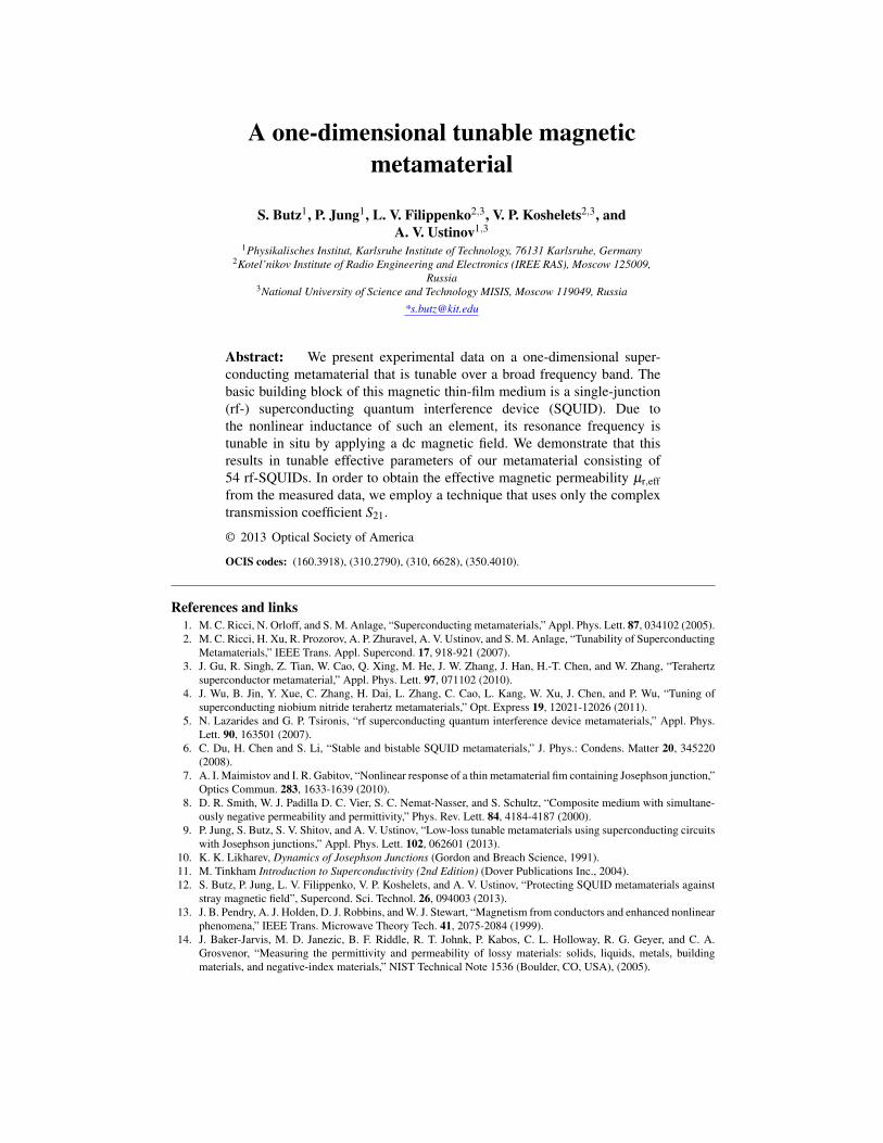
The basic building block of the metamaterial used in this work is a single junction (rf-)SQUID.Such an rf-SQUID consists of a superconducting loop interrupted by a Josephson junction (cf.Fig. 1(a)). The junction is indicated by a red cross.

Fig. 1. (a) Sketch of an rf-SQUID. The red cross symbolizes the Josephson junction.(b) Electric equivalent circuit for an rf-SQUID in the small signal approximation. Lgeois the geometric inductance of the SQUID loop. The red circle indicates the electric cir-cuit model for the junction. R represents the resistance due to a quasiparticle current, Lj isthe Josephson inductance and C stands for the capacitance between the superconductingelectrodes. (c) Optical micrograph of the rf-SQUID.

Within a small signal approximation, the Josephson junction can be considered as a nonlinearinductor [10, 11]. When placed inside a superconducting loop, this so-called Josephson induc-tance Lj is tunable by a magnetic field. In addition to Lj, the geometric inductance of the loopLgeo contributes to the total inductance Ltot of the rf-SQUID. The full equivalent electric cir-cuit is depicted in Fig. 1(b). The red circle marks the electric circuit analogue of the Josephsonjunction for which the resistively capacitively shunted junction model is used [11]. Like theSRR, the rf-SQUID can be interpreted as an LC-oscillator. Unlike the SRR however, the total


inductance and thus the resonance frequency of the rf-SQUID is tunable, assuming that the acmagnetic field component is small.

Figure 1(c) shows an optical micrograph of the single rf-SQUID. The SQUID and its junctionare fabricated using a Nb/AlOx/Nb trilayer process. The Josephson junction is circular with adiameter of 1.6 µm, its critical current Ic = 1.8 µA. From this value, the zero field Josephsoninductance is calculated to be Lj = 183 pH. This value is approximately twice as large as thegeometric inductance of the loop Lgeo = 82.5 pH. Thus, the rf-SQUID considered in this workis nonhysteretic [10, 11]. The junction is shunted with an additional parallel plate capacitorwith a capacitance Cshunt = 2.0 pF which is two orders of magnitude larger than the intrinsiccapacitance of the Josephson junction. Due to this shunt capacitor, the resonance frequency ofthe rf-SQUID is reduced and tunable between approximately 9 GHz and 15 GHz.

3. The SQUID Metamaterial

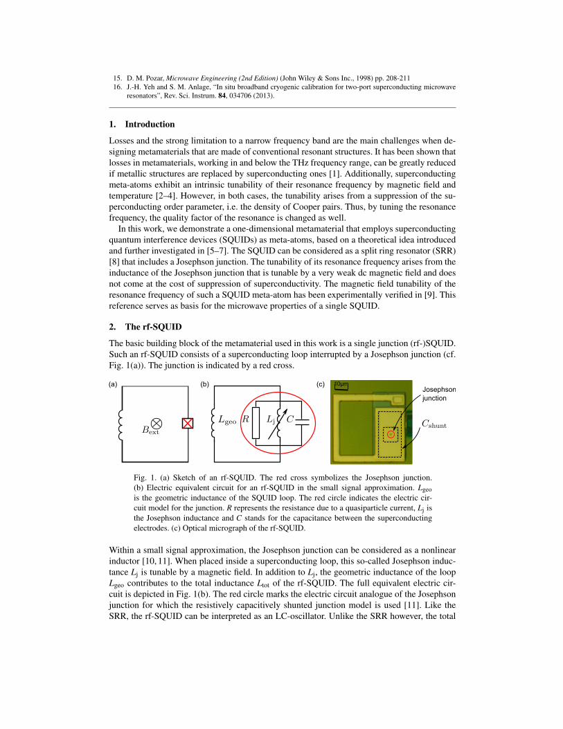
Two one-dimensional arrays of 27 rf-SQUIDs are placed inside the gaps of a coplanar wave-guide (CPW) as shown in Fig. 2(a). The CPW is fabricated in a planar geometry on a flatsubstrate and consists of a central conductor (dark green in Fig. 2(a)) and two ground planes(large light green areas in Fig. 2(a)). When only the two dimensional plane containing thewaveguide is considered, the electric and magnetic field components are located inside the twogaps (brown) between central conductor and ground planes. However, in three dimensions themagnetic field lines are closed loops around the central conductor. The waveguide enhances thecoupling between electromagnetic wave and the SQUIDs compared to the coupling to a free-space electromagnetic wave. In addition to the microwave signal, a dc current is applied alongthe central conductor, creating the dc magnetic field used to tune the resonance frequency. Dueto the waveguide geometry, the SQUIDs are oriented with their loop area perpendicular to themagnetic field.

The pitch between neighboring SQUIDs is much smaller than the wavelength. In this samplethe pitch is 92 µm, which is twice the width of the single SQUID and more than ten timesthe distance between each SQUID and the central conductor of the waveguide. Therefore, theinductive coupling between adjacent SQUIDs is approximately one order of magnitude smallerthan the coupling to the CPW and can be neglected.

Fig. 2. (a) Optical micrograph of part of the CPW containing a chain of rf-SQUIDs in eachgap. (b) Measurement setup including the vector network analyzer (VNA), the bias tees,attenuation and cryogenic amplifier. The green box marks the position of the the part of thewaveguide shown in the optical micrograph in (a).

The CPW is connected to a vector network analyzer (VNA) using coaxial cables. The fullexperimental setup is depicted in Fig. 2(b). The bias tees are used to superpose the microwavesignal with the dc current. Rigorous magnetic shielding (not shown in the picture) proved tobe crucial in order to protect the sample from stray magnetic fields originating from electronic


components in the setup [12]. The sample inside the cryoperm magnetic shield, part of theattenuation and the amplifier are placed in liquid helium at a temperature of T = 4.2 K.

4. Experimental Results

We measure the complex transmission through the CPW (S21) as a function of frequency ν

and magnetic flux Φe0. The microwave power at the sample is approximately P ≈ −90 dBm,including losses in the coaxial cables. The calibration of the measurement is done by applyinga flux of Φe0 = Φcal = Φ0/2. At this flux value the resonance frequency is shifted to its lowestpossible value, which lies between 9 and 10 GHz. The built-in “thru” calibration function of theVNA is used to subtract the corresponding reference data from the rest of the measurement (seealso Appendix B). The resulting transmission magnitude for such a measurement is presentedin Fig. 3. For clarity, only data above 10 GHz are shown.

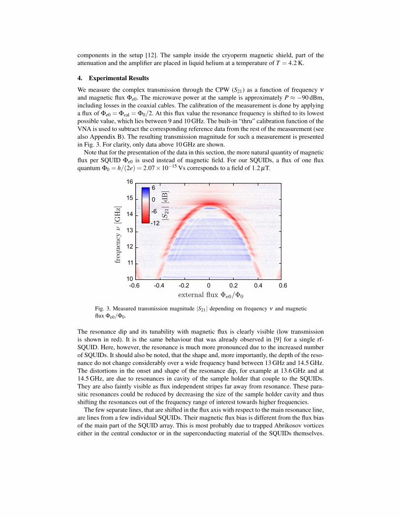
Note that for the presentation of the data in this section, the more natural quantity of magneticflux per SQUID Φe0 is used instead of magnetic field. For our SQUIDs, a flux of one fluxquantum Φ0 = h/(2e) = 2.07×10−15 Vs corresponds to a field of 1.2 µT.

Fig. 3. Measured transmission magnitude |S21| depending on frequency ν and magneticflux Φe0/Φ0.

The resonance dip and its tunability with magnetic flux is clearly visible (low transmissionis shown in red). It is the same behaviour that was already observed in [9] for a single rf-SQUID. Here, however, the resonance is much more pronounced due to the increased numberof SQUIDs. It should also be noted, that the shape and, more importantly, the depth of the reso-nance do not change considerably over a wide frequency band between 13 GHz and 14.5 GHz.The distortions in the onset and shape of the resonance dip, for example at 13.6 GHz and at14.5 GHz, are due to resonances in cavity of the sample holder that couple to the SQUIDs.They are also faintly visible as flux independent stripes far away from resonance. These para-sitic resonances could be reduced by decreasing the size of the sample holder cavity and thusshifting the resonances out of the frequency range of interest towards higher frequencies.

The few separate lines, that are shifted in the flux axis with respect to the main resonance line,are lines from a few individual SQUIDs. Their magnetic flux bias is different from the flux biasof the main part of the SQUID array. This is most probably due to trapped Abrikosov vorticeseither in the central conductor or in the superconducting material of the SQUIDs themselves.


By further improving the magnetic shielding and replacing the microwave cables that connectdirectly to the sample with non magnetic cables, the effect of stray magnetic fields could befurther suppressed.

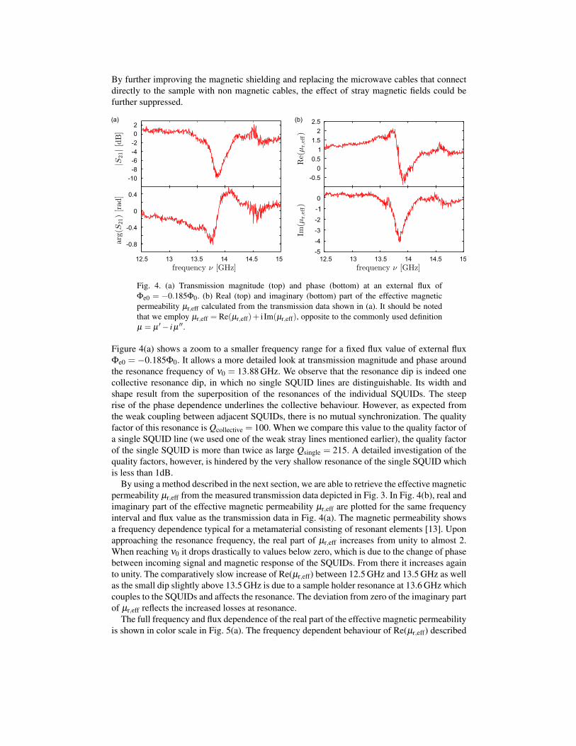
Fig. 4. (a) Transmission magnitude (top) and phase (bottom) at an external flux ofΦe0 = −0.185Φ0. (b) Real (top) and imaginary (bottom) part of the effective magneticpermeability µr,eff calculated from the transmission data shown in (a). It should be notedthat we employ µr,eff = Re(µr,eff)+ i Im(µr,eff), opposite to the commonly used definitionµ = µ ′− i µ ′′.

Figure 4(a) shows a zoom to a smaller frequency range for a fixed flux value of external fluxΦe0 = −0.185Φ0. It allows a more detailed look at transmission magnitude and phase aroundthe resonance frequency of ν0 = 13.88 GHz. We observe that the resonance dip is indeed onecollective resonance dip, in which no single SQUID lines are distinguishable. Its width andshape result from the superposition of the resonances of the individual SQUIDs. The steeprise of the phase dependence underlines the collective behaviour. However, as expected fromthe weak coupling between adjacent SQUIDs, there is no mutual synchronization. The qualityfactor of this resonance is Qcollective = 100. When we compare this value to the quality factor ofa single SQUID line (we used one of the weak stray lines mentioned earlier), the quality factorof the single SQUID is more than twice as large Qsingle = 215. A detailed investigation of thequality factors, however, is hindered by the very shallow resonance of the single SQUID whichis less than 1dB.

By using a method described in the next section, we are able to retrieve the effective magneticpermeability µr,eff from the measured transmission data depicted in Fig. 3. In Fig. 4(b), real andimaginary part of the effective magnetic permeability µr,eff are plotted for the same frequencyinterval and flux value as the transmission data in Fig. 4(a). The magnetic permeability showsa frequency dependence typical for a metamaterial consisting of resonant elements [13]. Uponapproaching the resonance frequency, the real part of µr,eff increases from unity to almost 2.When reaching ν0 it drops drastically to values below zero, which is due to the change of phasebetween incoming signal and magnetic response of the SQUIDs. From there it increases againto unity. The comparatively slow increase of Re(µr,eff) between 12.5 GHz and 13.5 GHz as wellas the small dip slightly above 13.5 GHz is due to a sample holder resonance at 13.6 GHz whichcouples to the SQUIDs and affects the resonance. The deviation from zero of the imaginary partof µr,eff reflects the increased losses at resonance.

The full frequency and flux dependence of the real part of the effective magnetic permeabilityis shown in color scale in Fig. 5(a). The frequency dependent behaviour of Re(µr,eff) described


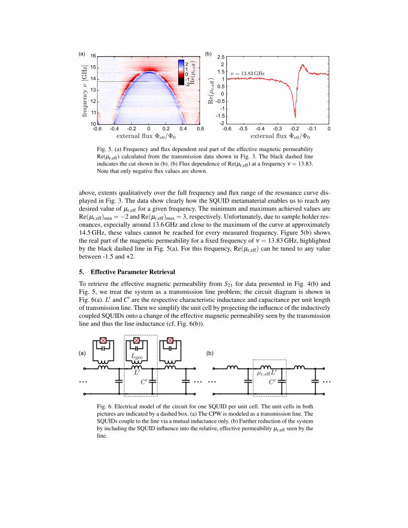
Fig. 5. (a) Frequency and flux dependent real part of the effective magnetic permeabilityRe(µr,eff) calculated from the transmission data shown in Fig. 3. The black dashed lineindicates the cut shown in (b). (b) Flux dependence of Re(µr,eff) at a frequency ν = 13.83.Note that only negative flux values are shown.

above, extents qualitatively over the full frequency and flux range of the resonance curve dis-played in Fig. 3. The data show clearly how the SQUID metamaterial enables us to reach anydesired value of µr,eff for a given frequency. The minimum and maximum achieved values areRe(µr,eff)min =−2 and Re(µr,eff)max = 3, respectively. Unfortunately, due to sample holder res-onances, especially around 13.6 GHz and close to the maximum of the curve at approximately14.5 GHz, these values cannot be reached for every measured frequency. Figure 5(b) showsthe real part of the magnetic permeability for a fixed frequency of ν = 13.83 GHz, highlightedby the black dashed line in Fig. 5(a). For this frequency, Re(µr,eff) can be tuned to any valuebetween -1.5 and +2.

5. Effective Parameter Retrieval

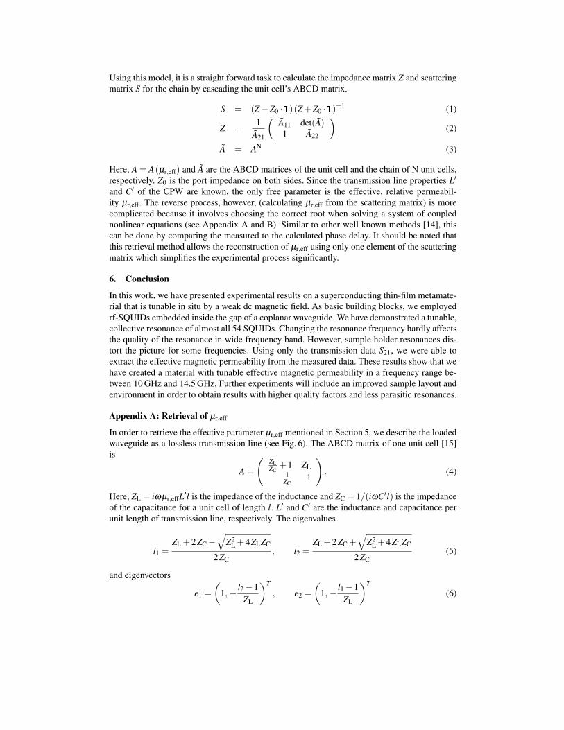
To retrieve the effective magnetic permeability from S21 for data presented in Fig. 4(b) andFig. 5, we treat the system as a transmission line problem; the circuit diagram is shown inFig. 6(a). L′ and C′ are the respective characteristic inductance and capacitance per unit lengthof transmission line. Then we simplify the unit cell by projecting the influence of the inductivelycoupled SQUIDs onto a change of the effective magnetic permeability seen by the transmissionline and thus the line inductance (cf. Fig. 6(b)).

Fig. 6. Electrical model of the circuit for one SQUID per unit cell. The unit cells in bothpictures are indicated by a dashed box. (a) The CPW is modeled as a transmission line. TheSQUIDs couple to the line via a mutual inductance only. (b) Further reduction of the systemby including the SQUID influence into the relative, effective permeability µr,eff seen by theline.


Using this model, it is a straight forward task to calculate the impedance matrix Z and scatteringmatrix S for the chain by cascading the unit cell’s ABCD matrix.

S = (Z−Z0 ·1)(Z +Z0 ·1)−1 (1)

Z =1

A21

(A11 det(A)1 A22

)(2)

A = AN (3)

Here, A = A(µr,eff) and A are the ABCD matrices of the unit cell and the chain of N unit cells,respectively. Z0 is the port impedance on both sides. Since the transmission line properties L′

and C′ of the CPW are known, the only free parameter is the effective, relative permeabil-ity µr,eff. The reverse process, however, (calculating µr,eff from the scattering matrix) is morecomplicated because it involves choosing the correct root when solving a system of couplednonlinear equations (see Appendix A and B). Similar to other well known methods [14], thiscan be done by comparing the measured to the calculated phase delay. It should be noted thatthis retrieval method allows the reconstruction of µr,eff using only one element of the scatteringmatrix which simplifies the experimental process significantly.

6. Conclusion

In this work, we have presented experimental results on a superconducting thin-film metamate-rial that is tunable in situ by a weak dc magnetic field. As basic building blocks, we employedrf-SQUIDs embedded inside the gap of a coplanar waveguide. We have demonstrated a tunable,collective resonance of almost all 54 SQUIDs. Changing the resonance frequency hardly affectsthe quality of the resonance in wide frequency band. However, sample holder resonances dis-tort the picture for some frequencies. Using only the transmission data S21, we were able toextract the effective magnetic permeability from the measured data. These results show that wehave created a material with tunable effective magnetic permeability in a frequency range be-tween 10 GHz and 14.5 GHz. Further experiments will include an improved sample layout andenvironment in order to obtain results with higher quality factors and less parasitic resonances.

Appendix A: Retrieval of µr,eff

In order to retrieve the effective parameter µr,eff mentioned in Section 5, we describe the loadedwaveguide as a lossless transmission line (see Fig. 6). The ABCD matrix of one unit cell [15]is

A =

(ZLZC

+1 ZL1

ZC1

). (4)

Here, ZL = iωµr,effL′l is the impedance of the inductance and ZC = 1/(iωC′l) is the impedanceof the capacitance for a unit cell of length l. L′ and C′ are the inductance and capacitance perunit length of transmission line, respectively. The eigenvalues

l1 =ZL +2ZC−

√Z2

L +4ZLZC

2ZC, l2 =

ZL +2ZC +√

Z2L +4ZLZC

2ZC(5)

and eigenvectors

e1 =

(1,− l2−1

ZL

)T

, e2 =

(1,− l1−1

ZL

)T

(6)


of the ABCD matrix can be used to rewrite it in the form

A =C ·(

l1 00 l2

)·C−1 (7)

with C =(

e1,e2). (8)

This simplifies the total ABCD matrix A when cascading N unit cells:

A = AN =C ·(

lN1 00 lN

2

)·C−1. (9)

Using this equation and the well-known relation [15] of A to the scattering matrix S, we con-struct a system of four coupled, nonlinear equations

0 =

− (l2−1)lN2 −(l1−1)lN

1l1−l2

(lN1 −lN

2 )ZLl1−l2

− (l1−1)lN1 l2−(l1−1)lN

1 −((l1−1)l2−l1+1)lN2

(l1−l2)ZL

(l1−1)lN2 −lN

1 l2+lN1

l1−l2

− (10)

(− (S11+1)S22−S12S21−S11−1

2S21

((S11+1)S22−S12S21+S11+1)Z02S21

(S11−1)S22−S12S21−S11+12S21Z0

− (S11−1)S22−S12S21+S11−12S21

)

for the four variables S11, S12, S22, and µr,eff since S21 is the measured quantity and all otherparameters (like L′ and C′) are known from either design considerations or simulations.In general, this system of equations is not single-valued. There are several ways to sort out im-plausible solutions like requiring reciprocity, energy conservation or comparing the measuredto the calculated phase delay.

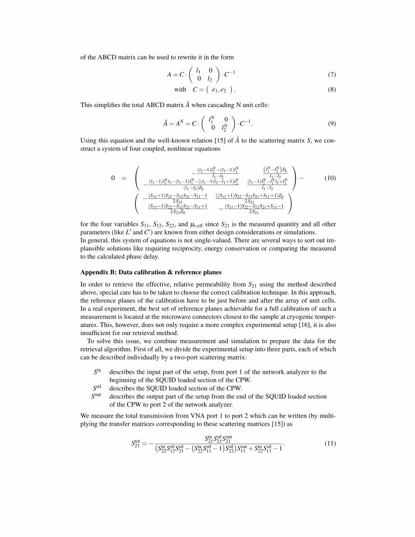
Appendix B: Data calibration & reference planes

In order to retrieve the effective, relative permeability from S21 using the method describedabove, special care has to be taken to choose the correct calibration technique. In this approach,the reference planes of the calibration have to be just before and after the array of unit cells.In a real experiment, the best set of reference planes achievable for a full calibration of such ameasurement is located at the microwave connectors closest to the sample at cryogenic temper-atures. This, however, does not only require a more complex experimental setup [16], it is alsoinsufficient for our retrieval method.

To solve this issue, we combine measurement and simulation to prepare the data for theretrieval algorithm. First of all, we divide the experimental setup into three parts, each of whichcan be described individually by a two-port scattering matrix:

Sin describes the input part of the setup, from port 1 of the network analyzer to thebeginning of the SQUID loaded section of the CPW.

Sstl describes the SQUID loaded section of the CPW.Sout describes the output part of the setup from the end of the SQUID loaded section

of the CPW to port 2 of the network analyzer.

We measure the total transmission from VNA port 1 to port 2 which can be written (by multi-plying the transfer matrices corresponding to these scattering matrices [15]) as

Stot21 =−

Sin21Sstl

21Sout21(

Sin22Sstl

12Sstl21−

(Sin

22Sstl11−1

)Sstl

22

)Sout

11 +Sin22Sstl

11−1. (11)


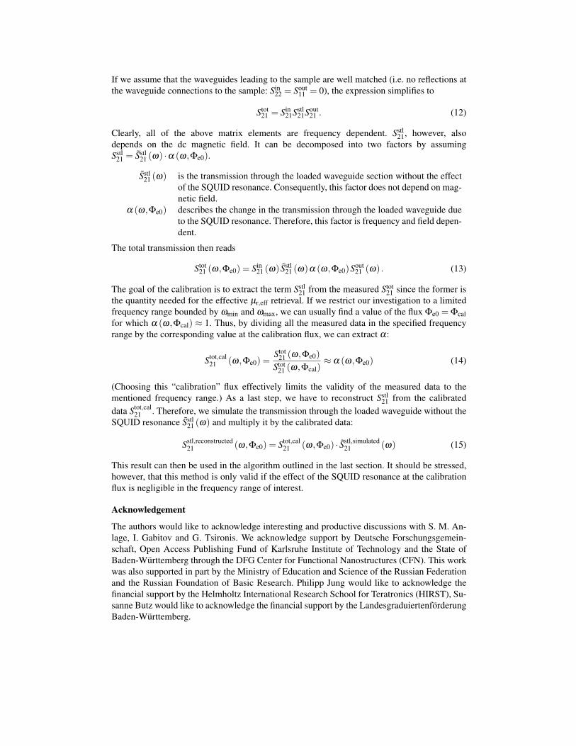
If we assume that the waveguides leading to the sample are well matched (i.e. no reflections atthe waveguide connections to the sample: Sin

22 = Sout11 = 0), the expression simplifies to

Stot21 = Sin

21Sstl21Sout

21 . (12)

Clearly, all of the above matrix elements are frequency dependent. Sstl21, however, also

depends on the dc magnetic field. It can be decomposed into two factors by assumingSstl

21 = Sstl21 (ω) ·α (ω,Φe0).

Sstl21 (ω) is the transmission through the loaded waveguide section without the effect

of the SQUID resonance. Consequently, this factor does not depend on mag-netic field.

α (ω,Φe0) describes the change in the transmission through the loaded waveguide dueto the SQUID resonance. Therefore, this factor is frequency and field depen-dent.

The total transmission then reads

Stot21 (ω,Φe0) = Sin

21 (ω) Sstl21 (ω)α (ω,Φe0)Sout

21 (ω) . (13)

The goal of the calibration is to extract the term Sstl21 from the measured Stot

21 since the former isthe quantity needed for the effective µr,eff retrieval. If we restrict our investigation to a limitedfrequency range bounded by ωmin and ωmax, we can usually find a value of the flux Φe0 = Φcalfor which α (ω,Φcal) ≈ 1. Thus, by dividing all the measured data in the specified frequencyrange by the corresponding value at the calibration flux, we can extract α:

Stot,cal21 (ω,Φe0) =

Stot21 (ω,Φe0)

Stot21 (ω,Φcal)

≈ α (ω,Φe0) (14)

(Choosing this “calibration” flux effectively limits the validity of the measured data to thementioned frequency range.) As a last step, we have to reconstruct Sstl

21 from the calibrateddata Stot,cal

21 . Therefore, we simulate the transmission through the loaded waveguide without theSQUID resonance Sstl

21 (ω) and multiply it by the calibrated data:

Sstl,reconstructed21 (ω,Φe0) = Stot,cal

21 (ω,Φe0) · Sstl,simulated21 (ω) (15)

This result can then be used in the algorithm outlined in the last section. It should be stressed,however, that this method is only valid if the effect of the SQUID resonance at the calibrationflux is negligible in the frequency range of interest.

Acknowledgement

The authors would like to acknowledge interesting and productive discussions with S. M. An-lage, I. Gabitov and G. Tsironis. We acknowledge support by Deutsche Forschungsgemein-schaft, Open Access Publishing Fund of Karlsruhe Institute of Technology and the State ofBaden-Wurttemberg through the DFG Center for Functional Nanostructures (CFN). This workwas also supported in part by the Ministry of Education and Science of the Russian Federationand the Russian Foundation of Basic Research. Philipp Jung would like to acknowledge thefinancial support by the Helmholtz International Research School for Teratronics (HIRST), Su-sanne Butz would like to acknowledge the financial support by the LandesgraduiertenforderungBaden-Wurttemberg.


Documents

A one-dimensional tunable magnetic metamaterial - Optics InfoBase