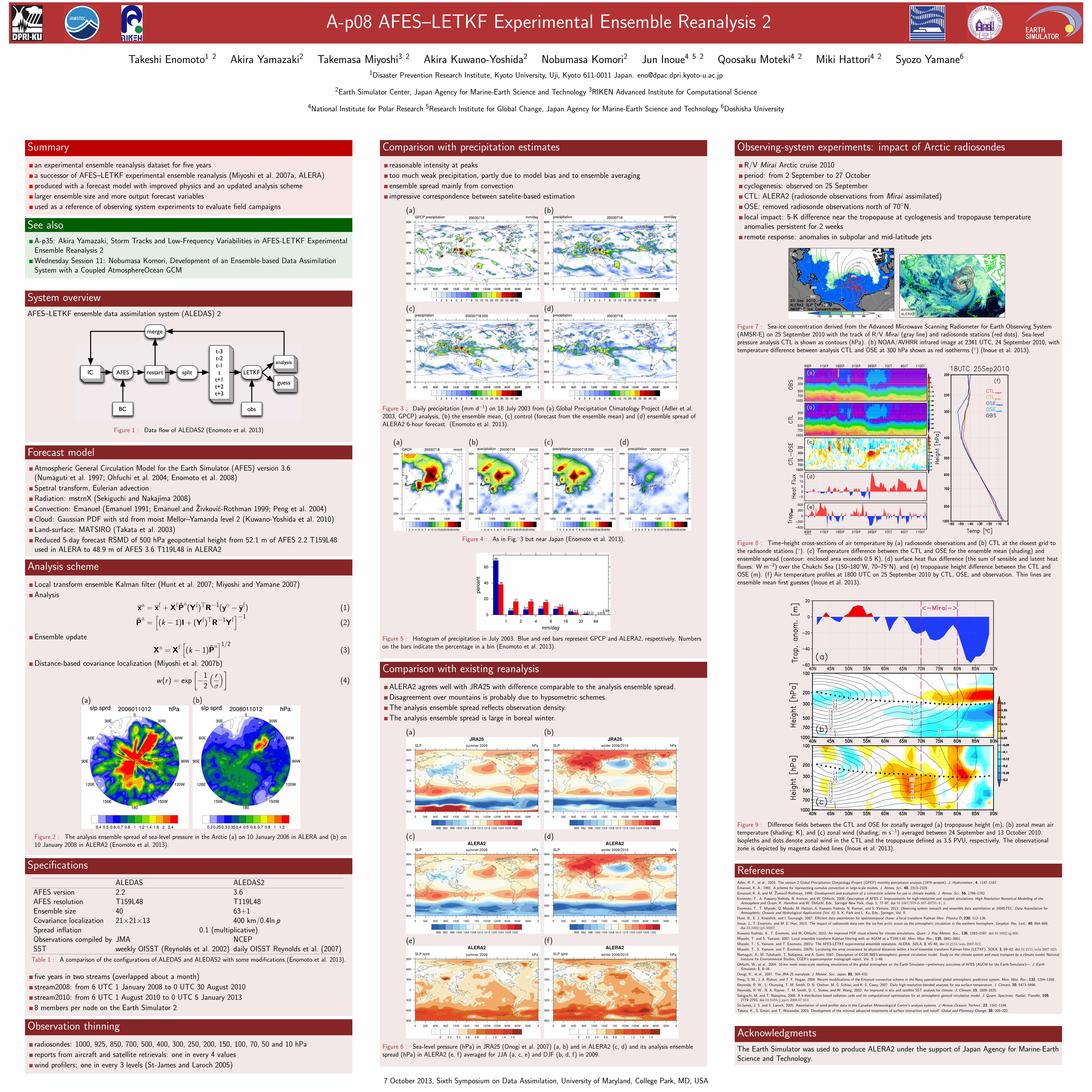
A-p08 AFES–LETKF Experimental Ensemble Reanalysis 2

Takeshi Enomoto1 2 Akira Yamazaki2 Takemasa Miyoshi3 2 Akira Kuwano-Yoshida2 Nobumasa Komori2 Jun Inoue4 5 2 Qoosaku Moteki4 2 Miki Hattori4 2 Syozo Yamane6

1Disaster Prevention Research Institute, Kyoto University, Uji, Kyoto 611-0011 Japan. eno@dpac.dpri.kyoto-u.ac.jp

2Earth Simulator Center, Japan Agency for Marine-Earth Science and Technology 3RIKEN Advanced Institute for Computational Science

4National Institute for Polar Research 5Research Institute for Global Change, Japan Agency for Marine-Earth Science and Technology 6Doshisha University

Summary

an experimental ensemble reanalysis dataset for five yearsa successor of AFES–LETKF experimental ensemble reanalysis (Miyoshi et al. 2007a, ALERA)produced with a forecast model with improved physics and an updated analysis schemelarger ensemble size and more output forecast variablesused as a reference of observing system experiments to evaluate field campaigns

See alsoA-p35: Akira Yamazaki, Storm Tracks and Low-Frequency Variabilities in AFES-LETKF ExperimentalEnsemble Reanalysis 2Wednesday Session 11: Nobumasa Komori, Development of an Ensemble-based Data AssimilationSystem with a Coupled AtmosphereOcean GCM

System overview

AFES–LETKF ensemble data assimilation system (ALEDAS) 2

AFES restartIC

t-3t-2t-1tt+1t+2t+3

merge

split

analysis

guess

LETKF

BC obs

Figure 1 : Data flow of ALEDAS2 (Enomoto et al. 2013)

Forecast modelAtmospheric General Circulation Model for the Earth Simulator (AFES) version 3.6(Numaguti et al. 1997; Ohfuchi et al. 2004; Enomoto et al. 2008)Spetral transform, Eulerian advectionRadiation: mstrnX (Sekiguchi and Nakajima 2008)Convection: Emanuel (Emanuel 1991; Emanuel and Zivkovic-Rothman 1999; Peng et al. 2004)Cloud: Gaussian PDF with std from moist Mellor–Yamanda level 2 (Kuwano-Yoshida et al. 2010)Land-surface: MATSIRO (Takata et al. 2003)Reduced 5-day forecast RSMD of 500 hPa geopotential height from 52.1 m of AFES 2.2 T159L48used in ALERA to 48.9 m of AFES 3.6 T119L48 in ALERA2

Analysis scheme

Local transform ensemble Kalman filter (Hunt et al. 2007; Miyoshi and Yamane 2007)Analysis

x

a = x

f + X

f

P

a

(Yf)TR�1(yo � y

f) (1)

P

a

=h(k � 1)I + (Yf)TR�1

Y

f

i�1(2)

Ensemble update

X

a = X

f

h(k � 1)P

a

i1/2(3)

Distance-based covariance localization (Miyoshi et al. 2007b)

w(r) = exp

�1

2

⇣ r�

⌘�(4)

(a) (b)

Figure 2 : The analysis ensemble spread of sea-level pressure in the Arctic (a) on 10 January 2006 in ALERA and (b) on10 January 2008 in ALERA2 (Enomoto et al. 2013).

Specifications

ALEDAS ALEDAS2AFES version 2.2 3.6AFES resolution T159L48 T119L48Ensemble size 40 63+1Covariance localization 21⇥21⇥13 400 km/0.4ln pSpread inflation 0.1 (multiplicative)Observations compiled by JMA NCEPSST weekly OISST (Reynolds et al. 2002) daily OISST Reynolds et al. (2007)Table 1 : A comparison of the configurations of ALEDAS and ALEDAS2 with some modifications (Enomoto et al. 2013).

five years in two streams (overlapped about a month)stream2008: from 6 UTC 1 January 2008 to 0 UTC 30 August 2010stream2010: from 6 UTC 1 August 2010 to 0 UTC 5 January 20138 members per node on the Earth Simulator 2

Observation thinning

radiosondes: 1000, 925, 850, 700, 500, 400, 300, 250, 200, 150, 100, 70, 50 and 10 hPareports from aircraft and satellite retrievals: one in every 4 valueswind profilers: one in every 3 levels (St-James and Laroch 2005)

Comparison with precipitation estimates

reasonable intensity at peakstoo much weak precipitation, partly due to model bias and to ensemble averagingensemble spread mainly from convectionimpressive correspondence between satelite-based estimation

(a) (b)

(c) (d)

Figure 3 : Daily precipitation (mm d�1) on 18 July 2003 from (a) Global Precipitation Climatology Project (Adler et al.2003, GPCP) analysis, (b) the ensemble mean, (c) control (forecast from the ensemble mean) and (d) ensemble spread ofALERA2 6-hour forecast. (Enomoto et al. 2013).

(a) (b) (c) (d)

Figure 4 : As in Fig. 3 but near Japan (Enomoto et al. 2013).

Figure 5 : Histogram of precipitation in July 2003. Blue and red bars represent GPCP and ALERA2, respectively. Numberson the bars indicate the percentage in a bin (Enomoto et al. 2013).

Comparison with existing reanalysis

ALERA2 agrees well with JRA25 with di↵erence comparable to the analysis ensemble spread.Disagreement over mountains is probably due to hypsometric schemes.The analysis ensemble spread reflects observation density.The analysis ensemble spread is large in boreal winter.

(a) (b)

(c) (d)

(e) (f)

Figure 6 : Sea-level pressure (hPa) in JRA25 (Onogi et al. 2007) (a, b) and in ALERA2 (c, d) and its analysis ensemblespread (hPa) in ALERA2 (e, f) averaged for JJA (a, c, e) and DJF (b, d, f) in 2009.

Observing-system experiments: impact of Arctic radiosondes

R/V Mirai Arctic cruise 2010period: from 2 September to 27 Octobercyclogenesis: observed on 25 SeptemberCTL: ALERA2 (radiosonde observations from Mirai assimilated)OSE: removed radiosonde observations north of 70�N.local impact: 5-K di↵erence near the tropopause at cyclogenesis and tropopause temperatureanomalies persistent for 2 weeksremote response: anomalies in subpolar and mid-latitude jets

Figure 7 : Sea-ice concentration derived from the Advanced Microwave Scanning Radiometer for Earth Observing System(AMSR-E) on 25 September 2010 with the track of R/V Mirai (gray line) and radiosonde stations (red dots). Sea-levelpressure analysis CTL is shown as contours (hPa). (b) NOAA/AVHRR infrared image at 2341 UTC, 24 September 2010, withtemperature di↵erence between analysis CTL and OSE at 300 hPa shown as red isotherms (�) (Inoue et al. 2013).

Figure 8 : Time–height cross-sections of air temperature by (a) radiosonde observations and (b) CTL at the closest grid tothe radisonde stations (�). (c) Temperature di↵erence between the CTL and OSE for the ensemble mean (shading) andensemble spread (contour: enclosed area exceeds 0.5 K), (d) surface heat flux di↵erence (the sum of sensible and latent heatfluxes: W m�2) over the Chukchi Sea (150–180�W, 70–75�N). and (e) tropopause height di↵erence between the CTL andOSE (m). (f) Air temperature profiles at 1800 UTC on 25 September 2010 by CTL, OSE, and observation. Thin lines areensemble mean first guesses (Inoue et al. 2013).

Figure 9 : Di↵erence fields between the CTL and OSE for zonally averaged (a) tropopause height (m), (b) zonal mean airtemperature (shading; K), and (c) zonal wind (shading; m s�1) averaged between 24 September and 13 October 2010.Isopleths and dots denote zonal wind in the CTL and the tropopause defined as 3.5 PVU, respectively. The observationalzone is depicted by magenta dashed lines (Inoue et al. 2013).

ReferencesAdler, R. F., et al., 2003: The version-2 Global Precipitation Climatology Project (GPCP) monthly precipitaion analysis (1979–present). J. Hydrometeor., 4, 1147–1167.

Emanuel, K. A., 1991: A scheme for representing cumulus convection in large-scale models. J. Atmos. Sci., 48, 2313–2329.

Emanuel, K. A. and M. Zivkovic-Rothman, 1999: Development and evaluation of a convection scheme for use in climate models. J. Atmos. Sci., 56, 1766–1782.

Enomoto, T., A. Kuwano-Yoshida, N. Komori, and W. Ohfuchi, 2008: Description of AFES 2: Improvements for high-resolution and coupled simulations. High Resolution Numerical Modelling of theAtmosphere and Ocean, K. Hamilton and W. Ohfuchi, Eds., Springer New York, chap. 5, 77–97, doi:10.1007/978-0-387-49791-4\ 5.

Enomoto, T., T. Miyoshi, Q. Moteki, M. Hattori, A. Kuwano-Yoshida, N. Komori, and S. Yamane, 2013: Observing-system research and ensemble data assimilation at JAMSTEC. Data Assimilation forAtmospheric, Oceanic and Hydrological Applications (Vol. II), S. K. Park and L. Xu, Eds., Springer, Vol. II.

Hunt, B., E. J. Kostelich, and I. Szunyogh, 2007: E�cient data assimilation for spatiotemporal chaos: a local transform Kalman filter. Physica D, 230, 112–126.

Inoue, J., T. Enomoto, and M. E. Hori, 2013: The impact of radiosonde data over the ice-free arctic ocean on the atmospheric circulation in the northern hemisphere. Geophys. Res. Lett., 40, 864–869,doi:10.1002/grl.50207.

Kuwano-Yoshida, A., T. Enomoto, and W. Ohfuchi, 2010: An improved PDF cloud scheme for climate simulations. Quart. J. Roy. Meteor. Soc., 136, 1583–1597, doi:10.1002/qj.660.

Miyoshi, T. and S. Yamane, 2007: Local ensemble transform Kalman filtering with an AGCM at a T159/L48. Mon. Wea. Rev., 135, 3841–3861.

Miyoshi, T., S. Yamane, and T. Enomoto, 2007a: The AFES-LETKF experimental ensemble reanalysis: ALERA. SOLA, 3, 45–48, doi:10.2151/sola.2007-012.

Miyoshi, T., S. Yamane, and T. Enomoto, 2007b: Localizing the error covariance by physical distances within a local ensemble transform Kalman filter (LETKF). SOLA, 3, 89–92, doi:10.2151/sola.2007-023.

Numaguti, A., M. Takahashi, T. Nakajima, and A. Sumi, 1997: Description of CCSR/NIES atmospheric general circulation model. Study on the climate system and mass transport by a climate model, NationalInstitute for Environmental Studies, CGER’s supercomputer monograph report, Vol. 3, 1–48.

Ohfuchi, W., et al., 2004: 10-km mesh meso-scale resolving simulations of the global atmosphere on the Earth Simulator—preliminary outcomes of AFES (AGCM for the Earth Simulator)—. J. EarthSimulator, 1, 8–34.

Onogi, K., et al., 2007: The JRA-25 reanalysis. J. Meteor. Soc. Japan, 85, 369–432.

Peng, S. M., J. A. Ridout, and T. F. Hogan, 2004: Recent modifications of the Emanuel convective scheme in the Navy operational global atmospheric prediction system. Mon. Wea. Rev., 132, 1254–1268.

Reynolds, R. W., L. Chunying, T. M. Smith, D. B. Chelton, M. G. Schlax, and K. S. Casey, 2007: Daily high-resolution-blended analyses for sea surface temperature. J. Climate, 20, 5473–5496.

Reynolds, R. W., N. A. Rayner, T. M. Smith, D. C. Stokes, and W. Wang, 2002: An improved in situ and satellite SST analysis for climate. J. Climate, 15, 1609–1625.

Sekiguchi, M. and T. Nakajima, 2008: A k-distribution-based radiation code and its computational optimization for an atmospheric general circulation model. J. Quant. Spectrosc. Radiat. Transfer, 109,2779–2793, doi:10.1016/j.jqsrt.2008.07.013.

St-James, J. S. and S. Laroch, 2005: Assimilation of wind profiler data in the Canadian Meteorological Centre’s analysis systems. J. Atmos. Oceanic Technol., 22, 1181–1194.

Takata, K., S. Emori, and T. Watanabe, 2003: Development of the minimal advanced treatments of surface interaction and runo↵. Global and Planetary Change, 38, 209–222.

Acknowledgments

The Earth Simulator was used to produce ALERA2 under the support of Japan Agency for Marine-EarthScience and Technology.

7 October 2013, Sixth Symposium on Data Assimilation, University of Maryland, College Park, MD, USA