A pragmatic and unified approach to CVA, PFE and … · A pragmatic and unified approach to CVA, PFE and VaR Robert Thorén, Head of Risk Solutions, Algorithmica Research . Overview

A pragmatic and unified approach to CVA, PFE and VaR

Robert Thorén, Head of Risk Solutions, Algorithmica Research

Overview

• Some definitions and questions to consider

• Going from PFE to CVA within the same calculation framework

• Some comments on computer implementation

• Questions and answers

12/4/2012 Algorithmica Research 2012 2

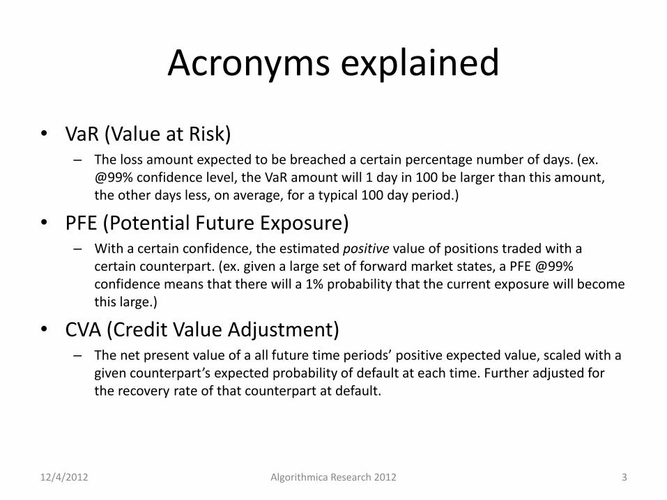
Acronyms explained

• VaR (Value at Risk) – The loss amount expected to be breached a certain percentage number of days. (ex.

@99% confidence level, the VaR amount will 1 day in 100 be larger than this amount, the other days less, on average, for a typical 100 day period.)

• PFE (Potential Future Exposure) – With a certain confidence, the estimated positive value of positions traded with a

certain counterpart. (ex. given a large set of forward market states, a PFE @99% confidence means that there will a 1% probability that the current exposure will become this large.)

• CVA (Credit Value Adjustment) – The net present value of a all future time periods’ positive expected value, scaled with a

given counterpart’s expected probability of default at each time. Further adjusted for the recovery rate of that counterpart at default.


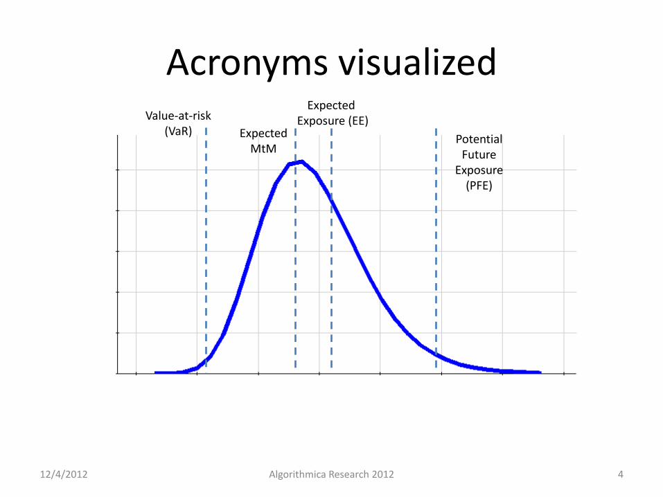
Acronyms visualized

Expected MtM

Expected Exposure (EE)

Potential Future

Exposure (PFE)

Value-at-risk (VaR)


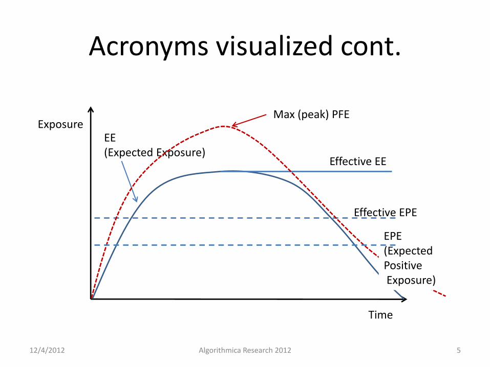
Acronyms visualized cont.

Time

Exposure EE (Expected Exposure)

Effective EE

Effective EPE

Max (peak) PFE

EPE (Expected Positive Exposure)


VaR, PFE & CVA similarities and differences

1) Given a non-parametric VaR model such as Historical Simulation, one needs historical samples to (re)price all positions.

2) Accepting historical simulation as model for forward looking risk implies; a) Wanting to use implied correlations (and not constant) b) That forward volatility can be guessed from the past c) An empirical distribution of returns (i.e. fat tails, skew, etc)

3) Why would a longer term forcast of Potential Future Exposure be underpinned by a different set of assumptions of the dynamics of market rates, quotes, etc? It should not. Same assumptions apply!

4) Calculation of CVA is dependent on calulation of the expected exposure. Could we take this directly from the PFE calculation?

-> Not exactly. CVA is the market price of counterparty risk, PFE and VaR are risk measures. Assuming you want to hedge CVA with market instruments, it needs to be calculated using risk neutral (market implied) assumptions.


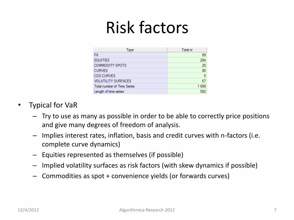
Risk factors

• Typical for VaR

– Try to use as many as possible in order to be able to correctly price positions and give many degrees of freedom of analysis.

– Implies interest rates, inflation, basis and credit curves with n-factors (i.e. complete curve dynamics)

– Equities represented as themselves (if possible)

– Implied volatility surfaces as risk factors (with skew dynamics if possible)

– Commodities as spot + convenience yields (or forwards curves)


Ok, assume we like our risk factor model ...

What kind of properties would we like to see for the representation of future market states in a multi-step forward simulation typical in a PFE real-world risk simulation? • To have yield-curves in forward states that remain arbitrage free, and “look plausible” • That the required relations between groups of market factors are maintained. For example, we seldom

want a BBB corporate spread to become narrower than the A spread, and the A spread should not be tighter than the AA spread and so on.

• A possibility to enforce mean-reversion in rates in order to avoid them from exploding on long time-horizons

• That the generated paths exhibit the same statistical properties as the real historical series, such as autocorrelation, kurtosis and correlations

• The ability to set drift terms that are in line with long term forward views on different asset classes and individual series

One method that will give this type of flexibility, while preserving observed features in historical market data, is bootstrapping, i.e. using the actual historical return data as the random number generator. These sample draws can then be stratified in order to re-create auto-correlation features. Yield curve nodes for each draw can be mildly “iid-perturbed”, creating a yield curve propagation that preserves the general and realistic shapes of the yield curve.


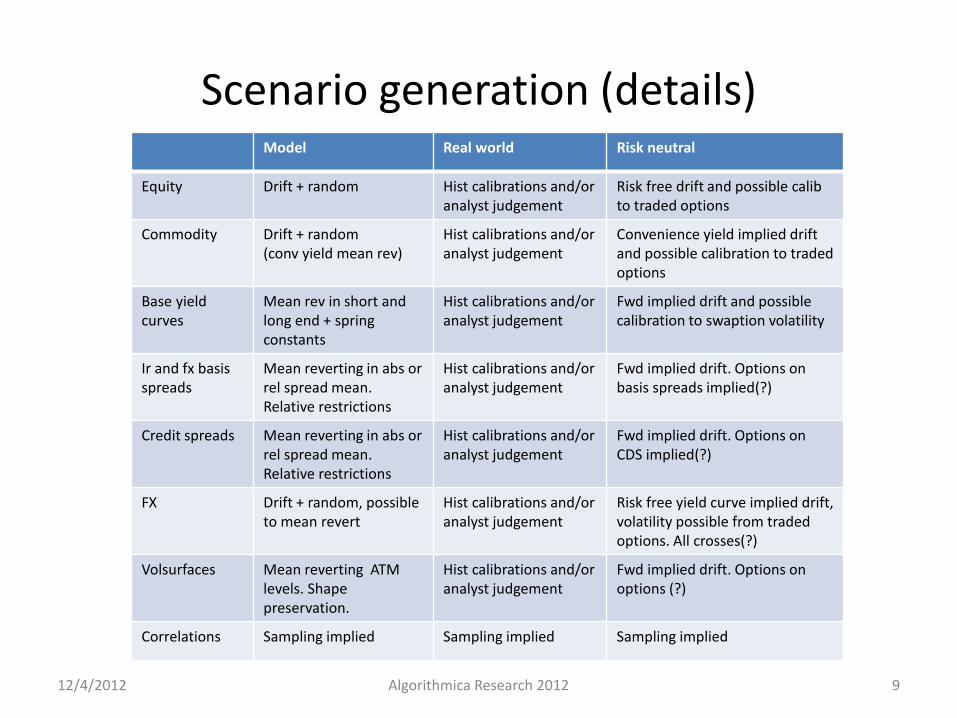
Scenario generation (details)

Model Real world Risk neutral

Equity Drift + random Hist calibrations and/or analyst judgement

Risk free drift and possible calib to traded options

Commodity Drift + random (conv yield mean rev)

Hist calibrations and/or analyst judgement

Convenience yield implied drift and possible calibration to traded options

Base yield curves

Mean rev in short and long end + spring constants


Fwd implied drift and possible calibration to swaption volatility

Ir and fx basis spreads

Mean reverting in abs or rel spread mean. Relative restrictions


Fwd implied drift. Options on basis spreads implied(?)

Credit spreads Mean reverting in abs or rel spread mean. Relative restrictions


Fwd implied drift. Options on CDS implied(?)

FX Drift + random, possible to mean revert


Risk free yield curve implied drift, volatility possible from traded options. All crosses(?)

Volsurfaces Mean reverting ATM levels. Shape preservation.


Fwd implied drift. Options on options (?)

Correlations Sampling implied Sampling implied Sampling implied


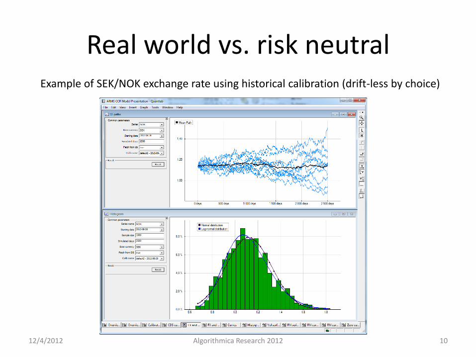
Real world vs. risk neutral Example of SEK/NOK exchange rate using historical calibration (drift-less by choice)


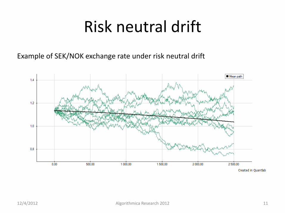
Risk neutral drift

Example of SEK/NOK exchange rate under risk neutral drift


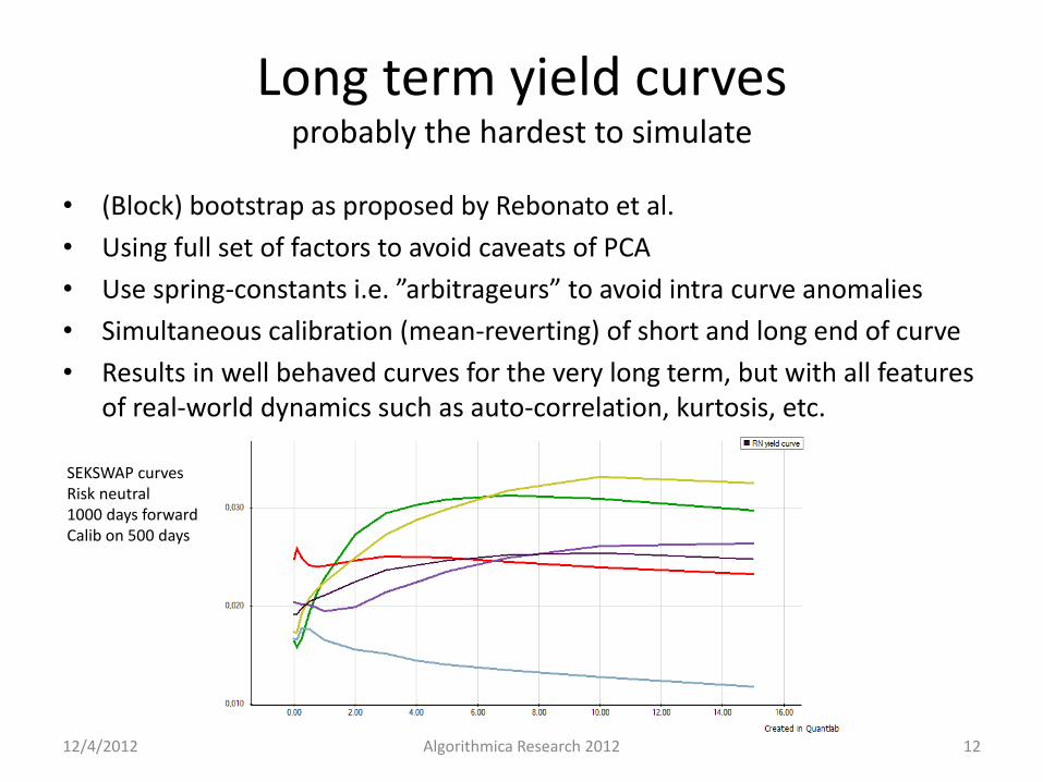
Long term yield curves probably the hardest to simulate

• (Block) bootstrap as proposed by Rebonato et al.

• Using full set of factors to avoid caveats of PCA

• Use spring-constants i.e. ”arbitrageurs” to avoid intra curve anomalies

• Simultaneous calibration (mean-reverting) of short and long end of curve

• Results in well behaved curves for the very long term, but with all features of real-world dynamics such as auto-correlation, kurtosis, etc.

SEKSWAP curves Risk neutral 1000 days forward Calib on 500 days


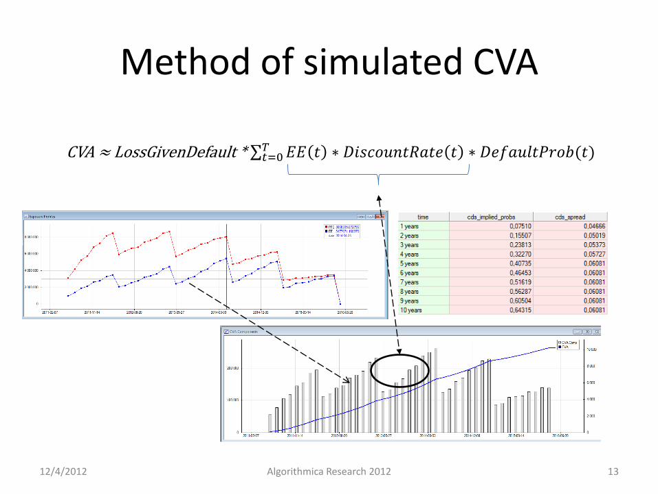
Method of simulated CVA

CVA ≈ LossGivenDefault * 𝐸𝐸 𝑡 ∗ 𝐷𝑖𝑠𝑐𝑜𝑢𝑛𝑡𝑅𝑎𝑡𝑒 𝑡 ∗ 𝐷𝑒𝑓𝑎𝑢𝑙𝑡𝑃𝑟𝑜𝑏(𝑡)𝑇𝑡=0


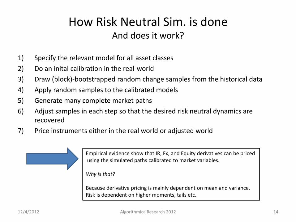
How Risk Neutral Sim. is done And does it work?

1) Specify the relevant model for all asset classes

2) Do an inital calibration in the real-world

3) Draw (block)-bootstrapped random change samples from the historical data

4) Apply random samples to the calibrated models

5) Generate many complete market paths

6) Adjust samples in each step so that the desired risk neutral dynamics are recovered

7) Price instruments either in the real world or adjusted world


Empirical evidence show that IR, Fx, and Equity derivatives can be priced using the simulated paths calibrated to market variables. Why is that? Because derivative pricing is mainly dependent on mean and variance. Risk is dependent on higher moments, tails etc.

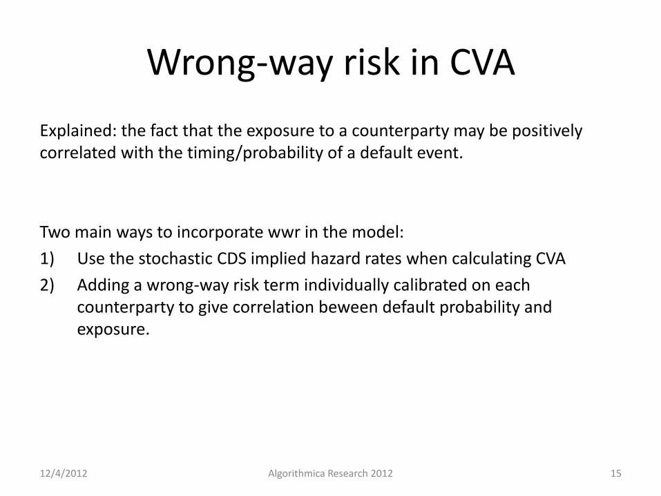
Wrong-way risk in CVA

Explained: the fact that the exposure to a counterparty may be positively correlated with the timing/probability of a default event.

Two main ways to incorporate wwr in the model:

1) Use the stochastic CDS implied hazard rates when calculating CVA

2) Adding a wrong-way risk term individually calibrated on each counterparty to give correlation beween default probability and exposure.


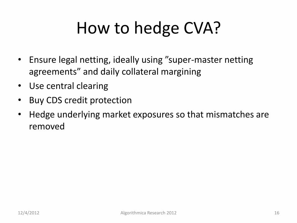
How to hedge CVA?

• Ensure legal netting, ideally using ”super-master netting agreements” and daily collateral margining

• Use central clearing

• Buy CDS credit protection

• Hedge underlying market exposures so that mismatches are removed


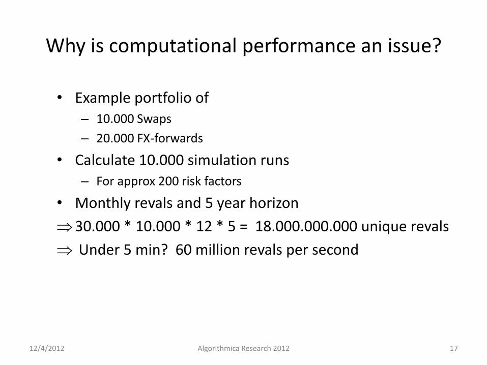
Why is computational performance an issue?

• Example portfolio of – 10.000 Swaps

– 20.000 FX-forwards

• Calculate 10.000 simulation runs – For approx 200 risk factors

• Monthly revals and 5 year horizon

30.000 * 10.000 * 12 * 5 = 18.000.000.000 unique revals

Under 5 min? 60 million revals per second


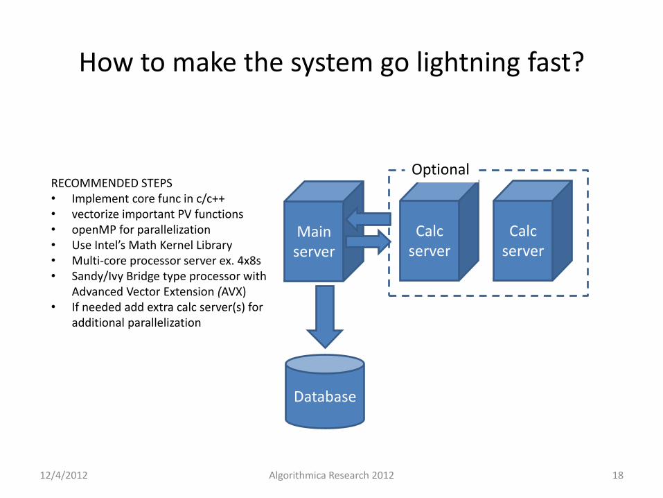
How to make the system go lightning fast?

Database

Calc server

Calc server

Main server

Optional RECOMMENDED STEPS • Implement core func in c/c++ • vectorize important PV functions • openMP for parallelization • Use Intel’s Math Kernel Library • Multi-core processor server ex. 4x8s • Sandy/Ivy Bridge type processor with

Advanced Vector Extension (AVX) • If needed add extra calc server(s) for

additional parallelization


Summary

• Benefits of having a unified model – Reuse of underlying risk factor data, assumptions, connection to

positions and system setup

• Calculation of PFE and CVA using either risk neutral or real world measure can be done simultaneous

• Correlation from history but not calibrated to the market; both good and bad

• Hedging market risk for VaR will have similar effect on PFE and CVA if within the same netting set.

• Stress-tesing on initial market data can be done concurrent for VaR, PFE and CVA.


Thank You! Q & A?


Documents

A pragmatic and unified approach to CVA, PFE and … · A pragmatic and unified approach to CVA, PFE and VaR Robert Thorén, Head of Risk Solutions, Algorithmica Research . Overview