Embed Size (px)
Citation preview
Tobias Nipkow Lawrence C. Paulson
Markus Wenzel
λ→
∀=Is
abelle
β
α
HOL
A Proof Assistant forHigher-Order Logic
August 15, 2018
Springer-Verlag
Berlin Heidelberg NewYorkLondon Paris TokyoHongKong BarcelonaBudapest

Preface
This volume is a self-contained introduction to interactive proof in higher-order logic (HOL), using the proof assistant Isabelle. It is written for potentialusers rather than for our colleagues in the research world.
The book has three parts.
– The first part, Elementary Techniques, shows how to model functionalprograms in higher-order logic. Early examples involve lists and the naturalnumbers. Most proofs are two steps long, consisting of induction on achosen variable followed by the auto tactic. But even this elementary partcovers such advanced topics as nested and mutual recursion.
– The second part, Logic and Sets, presents a collection of lower-leveltactics that you can use to apply rules selectively. It also describes Isa-belle/HOL’s treatment of sets, functions and relations and explains how todefine sets inductively. One of the examples concerns the theory of modelchecking, and another is drawn from a classic textbook on formal languages.
– The third part, Advanced Material, describes a variety of other topics.Among these are the real numbers, records and overloading. Advancedtechniques for induction and recursion are described. A whole chapter isdevoted to an extended example: the verification of a security protocol.
The typesetting relies on Wenzel’s theory presentation tools. An anno-tated source file is run, typesetting the theory in the form of a LATEX sourcefile. This book is derived almost entirely from output generated in this way.The final chapter of Part I explains how users may produce their own formaldocuments in a similar fashion.
Isabelle’s web site1 contains links to the download area and to documenta-tion and other information. The classic Isabelle user interface is Proof Gen-eral / Emacs by David Aspinall’s. This book says very little about ProofGeneral, which has its own documentation.
This tutorial owes a lot to the constant discussions with and the valuablefeedback from the Isabelle group at Munich: Stefan Berghofer, Olaf Muller,Wolfgang Naraschewski, David von Oheimb, Leonor Prensa Nieto, CorneliaPusch, Norbert Schirmer and Martin Strecker. Stephan Merz was also kind
1 https://isabelle.in.tum.de/

iv Preface
enough to read and comment on a draft version. We received comments fromStefano Bistarelli, Gergely Buday, John Matthews and Tanja Vos.
The research has been funded by many sources, including the dfggrants NI 491/2, NI 491/3, NI 491/4, NI 491/6, bmbf project Verisoft,the epsrc grants GR/K57381, GR/K77051, GR/M75440, GR/R01156/01GR/S57198/01 and by the esprit working groups 21900 and IST-1999-29001(the Types project).
Contents
Part I. Elementary Techniques
1. The Basics . . . . . . . . . . . . . . . . . . . . . . . . . . . . . . . . . . . . . . . . . . . . . . . . 31.1 Introduction . . . . . . . . . . . . . . . . . . . . . . . . . . . . . . . . . . . . . . . . . . . 31.2 Theories . . . . . . . . . . . . . . . . . . . . . . . . . . . . . . . . . . . . . . . . . . . . . . . 41.3 Types, Terms and Formulae . . . . . . . . . . . . . . . . . . . . . . . . . . . . . 41.4 Variables . . . . . . . . . . . . . . . . . . . . . . . . . . . . . . . . . . . . . . . . . . . . . . 71.5 Interaction and Interfaces . . . . . . . . . . . . . . . . . . . . . . . . . . . . . . . 71.6 Getting Started . . . . . . . . . . . . . . . . . . . . . . . . . . . . . . . . . . . . . . . . 8
2. Functional Programming in HOL . . . . . . . . . . . . . . . . . . . . . . . . . 92.1 An Introductory Theory . . . . . . . . . . . . . . . . . . . . . . . . . . . . . . . . . 92.2 Evaluation . . . . . . . . . . . . . . . . . . . . . . . . . . . . . . . . . . . . . . . . . . . . . 112.3 An Introductory Proof . . . . . . . . . . . . . . . . . . . . . . . . . . . . . . . . . . 122.4 Some Helpful Commands . . . . . . . . . . . . . . . . . . . . . . . . . . . . . . . . 162.5 Datatypes . . . . . . . . . . . . . . . . . . . . . . . . . . . . . . . . . . . . . . . . . . . . . 16
2.5.1 Lists . . . . . . . . . . . . . . . . . . . . . . . . . . . . . . . . . . . . . . . . . . . . 172.5.2 The General Format . . . . . . . . . . . . . . . . . . . . . . . . . . . . . . 172.5.3 Primitive Recursion . . . . . . . . . . . . . . . . . . . . . . . . . . . . . . 182.5.4 Case Expressions . . . . . . . . . . . . . . . . . . . . . . . . . . . . . . . . . 182.5.5 Structural Induction and Case Distinction . . . . . . . . . . . 192.5.6 Case Study: Boolean Expressions . . . . . . . . . . . . . . . . . . . 19
2.6 Some Basic Types . . . . . . . . . . . . . . . . . . . . . . . . . . . . . . . . . . . . . . 222.6.1 Natural Numbers . . . . . . . . . . . . . . . . . . . . . . . . . . . . . . . . . 222.6.2 Pairs . . . . . . . . . . . . . . . . . . . . . . . . . . . . . . . . . . . . . . . . . . . 232.6.3 Datatype option . . . . . . . . . . . . . . . . . . . . . . . . . . . . . . . . . 24
2.7 Definitions . . . . . . . . . . . . . . . . . . . . . . . . . . . . . . . . . . . . . . . . . . . . . 242.7.1 Type Synonyms . . . . . . . . . . . . . . . . . . . . . . . . . . . . . . . . . . 242.7.2 Constant Definitions . . . . . . . . . . . . . . . . . . . . . . . . . . . . . . 25
2.8 The Definitional Approach . . . . . . . . . . . . . . . . . . . . . . . . . . . . . . . 25
3. More Functional Programming . . . . . . . . . . . . . . . . . . . . . . . . . . . 273.1 Simplification . . . . . . . . . . . . . . . . . . . . . . . . . . . . . . . . . . . . . . . . . . 27
3.1.1 What is Simplification? . . . . . . . . . . . . . . . . . . . . . . . . . . . 273.1.2 Simplification Rules . . . . . . . . . . . . . . . . . . . . . . . . . . . . . . 28
vi Contents
3.1.3 The simp Method . . . . . . . . . . . . . . . . . . . . . . . . . . . . . . . . 283.1.4 Adding and Deleting Simplification Rules . . . . . . . . . . . 293.1.5 Assumptions . . . . . . . . . . . . . . . . . . . . . . . . . . . . . . . . . . . . . 293.1.6 Rewriting with Definitions . . . . . . . . . . . . . . . . . . . . . . . . . 303.1.7 Simplifying let-Expressions . . . . . . . . . . . . . . . . . . . . . . . 303.1.8 Conditional Simplification Rules . . . . . . . . . . . . . . . . . . . . 313.1.9 Automatic Case Splits . . . . . . . . . . . . . . . . . . . . . . . . . . . . 313.1.10 Tracing . . . . . . . . . . . . . . . . . . . . . . . . . . . . . . . . . . . . . . . . . 323.1.11 Finding Theorems . . . . . . . . . . . . . . . . . . . . . . . . . . . . . . . . 34
3.2 Induction Heuristics . . . . . . . . . . . . . . . . . . . . . . . . . . . . . . . . . . . . 353.3 Case Study: Compiling Expressions . . . . . . . . . . . . . . . . . . . . . . . 373.4 Advanced Datatypes . . . . . . . . . . . . . . . . . . . . . . . . . . . . . . . . . . . . 39
3.4.1 Mutual Recursion . . . . . . . . . . . . . . . . . . . . . . . . . . . . . . . . 393.4.2 Nested Recursion . . . . . . . . . . . . . . . . . . . . . . . . . . . . . . . . . 413.4.3 The Limits of Nested Recursion . . . . . . . . . . . . . . . . . . . . 433.4.4 Case Study: Tries . . . . . . . . . . . . . . . . . . . . . . . . . . . . . . . . 44
3.5 Total Recursive Functions: fun . . . . . . . . . . . . . . . . . . . . . . . . . . . 473.5.1 Definition . . . . . . . . . . . . . . . . . . . . . . . . . . . . . . . . . . . . . . . 483.5.2 Termination . . . . . . . . . . . . . . . . . . . . . . . . . . . . . . . . . . . . . 493.5.3 Simplification . . . . . . . . . . . . . . . . . . . . . . . . . . . . . . . . . . . . 493.5.4 Induction . . . . . . . . . . . . . . . . . . . . . . . . . . . . . . . . . . . . . . . . 50
4. Presenting Theories . . . . . . . . . . . . . . . . . . . . . . . . . . . . . . . . . . . . . . 534.1 Concrete Syntax . . . . . . . . . . . . . . . . . . . . . . . . . . . . . . . . . . . . . . . 53
4.1.1 Infix Annotations . . . . . . . . . . . . . . . . . . . . . . . . . . . . . . . . 534.1.2 Mathematical Symbols . . . . . . . . . . . . . . . . . . . . . . . . . . . 544.1.3 Prefix Annotations . . . . . . . . . . . . . . . . . . . . . . . . . . . . . . . 554.1.4 Abbreviations . . . . . . . . . . . . . . . . . . . . . . . . . . . . . . . . . . . 56
4.2 Document Preparation . . . . . . . . . . . . . . . . . . . . . . . . . . . . . . . . . 574.2.1 Isabelle Sessions . . . . . . . . . . . . . . . . . . . . . . . . . . . . . . . . . . 584.2.2 Structure Markup . . . . . . . . . . . . . . . . . . . . . . . . . . . . . . . . 594.2.3 Formal Comments and Antiquotations . . . . . . . . . . . . . . 604.2.4 Interpretation of Symbols . . . . . . . . . . . . . . . . . . . . . . . . . 624.2.5 Suppressing Output . . . . . . . . . . . . . . . . . . . . . . . . . . . . . . 63
Part II. Logic and Sets
5. The Rules of the Game . . . . . . . . . . . . . . . . . . . . . . . . . . . . . . . . . . . 675.1 Natural Deduction . . . . . . . . . . . . . . . . . . . . . . . . . . . . . . . . . . . . . . 675.2 Introduction Rules . . . . . . . . . . . . . . . . . . . . . . . . . . . . . . . . . . . . . . 685.3 Elimination Rules . . . . . . . . . . . . . . . . . . . . . . . . . . . . . . . . . . . . . . 695.4 Destruction Rules: Some Examples . . . . . . . . . . . . . . . . . . . . . . . 715.5 Implication . . . . . . . . . . . . . . . . . . . . . . . . . . . . . . . . . . . . . . . . . . . . 725.6 Negation . . . . . . . . . . . . . . . . . . . . . . . . . . . . . . . . . . . . . . . . . . . . . . 73
Contents vii
5.7 Interlude: the Basic Methods for Rules . . . . . . . . . . . . . . . . . . . . 755.8 Unification and Substitution . . . . . . . . . . . . . . . . . . . . . . . . . . . . . 76
5.8.1 Substitution and the subst Method . . . . . . . . . . . . . . . . 775.8.2 Unification and Its Pitfalls . . . . . . . . . . . . . . . . . . . . . . . . . 79
5.9 Quantifiers . . . . . . . . . . . . . . . . . . . . . . . . . . . . . . . . . . . . . . . . . . . . 805.9.1 The Universal Introduction Rule . . . . . . . . . . . . . . . . . . . 815.9.2 The Universal Elimination Rule . . . . . . . . . . . . . . . . . . . . 815.9.3 The Existential Quantifier . . . . . . . . . . . . . . . . . . . . . . . . . 825.9.4 Renaming a Bound Variable: rename_tac . . . . . . . . . . . 835.9.5 Reusing an Assumption: frule . . . . . . . . . . . . . . . . . . . . . 845.9.6 Instantiating a Quantifier Explicitly . . . . . . . . . . . . . . . . 84
5.10 Description Operators . . . . . . . . . . . . . . . . . . . . . . . . . . . . . . . . . . . 865.10.1 Definite Descriptions . . . . . . . . . . . . . . . . . . . . . . . . . . . . . . 865.10.2 Indefinite Descriptions . . . . . . . . . . . . . . . . . . . . . . . . . . . . 87
5.11 Some Proofs That Fail . . . . . . . . . . . . . . . . . . . . . . . . . . . . . . . . . . 885.12 Proving Theorems Using the blast Method. . . . . . . . . . . . . . . . 905.13 Other Classical Reasoning Methods . . . . . . . . . . . . . . . . . . . . . . . 915.14 Finding More Theorems . . . . . . . . . . . . . . . . . . . . . . . . . . . . . . . . . 935.15 Forward Proof: Transforming Theorems . . . . . . . . . . . . . . . . . . . 94
5.15.1 Modifying a Theorem using of, where and THEN . . . . . . 945.15.2 Modifying a Theorem using OF . . . . . . . . . . . . . . . . . . . . . 96
5.16 Forward Reasoning in a Backward Proof . . . . . . . . . . . . . . . . . . 975.16.1 The Method insert . . . . . . . . . . . . . . . . . . . . . . . . . . . . . . 985.16.2 The Method subgoal_tac . . . . . . . . . . . . . . . . . . . . . . . . . 99
5.17 Managing Large Proofs . . . . . . . . . . . . . . . . . . . . . . . . . . . . . . . . . . 1005.17.1 Tacticals, or Control Structures . . . . . . . . . . . . . . . . . . . . 1005.17.2 Subgoal Numbering . . . . . . . . . . . . . . . . . . . . . . . . . . . . . . . 101
5.18 Proving the Correctness of Euclid’s Algorithm . . . . . . . . . . . . . 103
6. Sets, Functions and Relations . . . . . . . . . . . . . . . . . . . . . . . . . . . . . 1076.1 Sets . . . . . . . . . . . . . . . . . . . . . . . . . . . . . . . . . . . . . . . . . . . . . . . . . . 107
6.1.1 Finite Set Notation . . . . . . . . . . . . . . . . . . . . . . . . . . . . . . . 1096.1.2 Set Comprehension . . . . . . . . . . . . . . . . . . . . . . . . . . . . . . . 1096.1.3 Binding Operators . . . . . . . . . . . . . . . . . . . . . . . . . . . . . . . . 1106.1.4 Finiteness and Cardinality . . . . . . . . . . . . . . . . . . . . . . . . . 111
6.2 Functions . . . . . . . . . . . . . . . . . . . . . . . . . . . . . . . . . . . . . . . . . . . . . . 1116.2.1 Function Basics . . . . . . . . . . . . . . . . . . . . . . . . . . . . . . . . . . 1116.2.2 Injections, Surjections, Bijections . . . . . . . . . . . . . . . . . . . 1126.2.3 Function Image . . . . . . . . . . . . . . . . . . . . . . . . . . . . . . . . . . 113
6.3 Relations . . . . . . . . . . . . . . . . . . . . . . . . . . . . . . . . . . . . . . . . . . . . . . 1136.3.1 Relation Basics . . . . . . . . . . . . . . . . . . . . . . . . . . . . . . . . . . 1146.3.2 The Reflexive and Transitive Closure . . . . . . . . . . . . . . . 1146.3.3 A Sample Proof . . . . . . . . . . . . . . . . . . . . . . . . . . . . . . . . . . 115
6.4 Well-Founded Relations and Induction . . . . . . . . . . . . . . . . . . . . 1166.5 Fixed Point Operators . . . . . . . . . . . . . . . . . . . . . . . . . . . . . . . . . . 117
viii Contents
6.6 Case Study: Verified Model Checking . . . . . . . . . . . . . . . . . . . . . 1186.6.1 Propositional Dynamic Logic — PDL . . . . . . . . . . . . . . . 1206.6.2 Computation Tree Logic — CTL . . . . . . . . . . . . . . . . . . . 123
7. Inductively Defined Sets . . . . . . . . . . . . . . . . . . . . . . . . . . . . . . . . . . 1297.1 The Set of Even Numbers . . . . . . . . . . . . . . . . . . . . . . . . . . . . . . . 129
7.1.1 Making an Inductive Definition . . . . . . . . . . . . . . . . . . . . 1297.1.2 Using Introduction Rules . . . . . . . . . . . . . . . . . . . . . . . . . . 1307.1.3 Rule Induction . . . . . . . . . . . . . . . . . . . . . . . . . . . . . . . . . . 1307.1.4 Generalization and Rule Induction . . . . . . . . . . . . . . . . . 1317.1.5 Rule Inversion . . . . . . . . . . . . . . . . . . . . . . . . . . . . . . . . . . . 1327.1.6 Mutually Inductive Definitions . . . . . . . . . . . . . . . . . . . . . 1347.1.7 Inductively Defined Predicates . . . . . . . . . . . . . . . . . . . . . 134
7.2 The Reflexive Transitive Closure . . . . . . . . . . . . . . . . . . . . . . . . . 1357.3 Advanced Inductive Definitions . . . . . . . . . . . . . . . . . . . . . . . . . . . 138
7.3.1 Universal Quantifiers in Introduction Rules . . . . . . . . . 1387.3.2 Alternative Definition Using a Monotone Function . . . . 1397.3.3 A Proof of Equivalence . . . . . . . . . . . . . . . . . . . . . . . . . . . . 1417.3.4 Another Example of Rule Inversion . . . . . . . . . . . . . . . . . 142
7.4 Case Study: A Context Free Grammar . . . . . . . . . . . . . . . . . . . . 143
Part III. Advanced Material
8. More about Types . . . . . . . . . . . . . . . . . . . . . . . . . . . . . . . . . . . . . . . . 1518.1 Pairs and Tuples . . . . . . . . . . . . . . . . . . . . . . . . . . . . . . . . . . . . . . . 151
8.1.1 Pattern Matching with Tuples . . . . . . . . . . . . . . . . . . . . . 1518.1.2 Theorem Proving . . . . . . . . . . . . . . . . . . . . . . . . . . . . . . . . . 152
8.2 Records . . . . . . . . . . . . . . . . . . . . . . . . . . . . . . . . . . . . . . . . . . . . . . 1548.2.1 Record Basics . . . . . . . . . . . . . . . . . . . . . . . . . . . . . . . . . . . . 1548.2.2 Extensible Records and Generic Operations . . . . . . . . . . 1558.2.3 Record Equality . . . . . . . . . . . . . . . . . . . . . . . . . . . . . . . . . . 1578.2.4 Extending and Truncating Records . . . . . . . . . . . . . . . . . 158
8.3 Type Classes . . . . . . . . . . . . . . . . . . . . . . . . . . . . . . . . . . . . . . . . . . . 1608.3.1 Overloading . . . . . . . . . . . . . . . . . . . . . . . . . . . . . . . . . . . . . 1608.3.2 Axioms . . . . . . . . . . . . . . . . . . . . . . . . . . . . . . . . . . . . . . . . . 161
8.4 Numbers . . . . . . . . . . . . . . . . . . . . . . . . . . . . . . . . . . . . . . . . . . . . . . 1658.4.1 Numeric Literals . . . . . . . . . . . . . . . . . . . . . . . . . . . . . . . . . 1668.4.2 The Type of Natural Numbers, nat . . . . . . . . . . . . . . . . . 1678.4.3 The Type of Integers, int . . . . . . . . . . . . . . . . . . . . . . . . . 1688.4.4 The Types of Rational, Real and Complex Numbers . . 1708.4.5 The Numeric Type Classes . . . . . . . . . . . . . . . . . . . . . . . . 170
8.5 Introducing New Types . . . . . . . . . . . . . . . . . . . . . . . . . . . . . . . . . 1738.5.1 Declaring New Types . . . . . . . . . . . . . . . . . . . . . . . . . . . . . 1738.5.2 Defining New Types . . . . . . . . . . . . . . . . . . . . . . . . . . . . . . 173
Contents ix
9. Advanced Simplification and Induction . . . . . . . . . . . . . . . . . . . 1779.1 Simplification . . . . . . . . . . . . . . . . . . . . . . . . . . . . . . . . . . . . . . . . . . 177
9.1.1 Advanced Features . . . . . . . . . . . . . . . . . . . . . . . . . . . . . . . 1779.1.2 How the Simplifier Works . . . . . . . . . . . . . . . . . . . . . . . . . 179
9.2 Advanced Induction Techniques . . . . . . . . . . . . . . . . . . . . . . . . . . 1809.2.1 Massaging the Proposition . . . . . . . . . . . . . . . . . . . . . . . . . 1809.2.2 Beyond Structural and Recursion Induction . . . . . . . . . . 1829.2.3 Derivation of New Induction Schemas . . . . . . . . . . . . . . . 1849.2.4 CTL Revisited . . . . . . . . . . . . . . . . . . . . . . . . . . . . . . . . . . . 184
10. Case Study: Verifying a Security Protocol . . . . . . . . . . . . . . . . 18910.1 The Needham-Schroeder Public-Key Protocol . . . . . . . . . . . . . . 18910.2 Agents and Messages . . . . . . . . . . . . . . . . . . . . . . . . . . . . . . . . . . . 19110.3 Modelling the Adversary . . . . . . . . . . . . . . . . . . . . . . . . . . . . . . . . 19210.4 Event Traces . . . . . . . . . . . . . . . . . . . . . . . . . . . . . . . . . . . . . . . . . . 19310.5 Modelling the Protocol . . . . . . . . . . . . . . . . . . . . . . . . . . . . . . . . . 19410.6 Proving Elementary Properties . . . . . . . . . . . . . . . . . . . . . . . . . . 19510.7 Proving Secrecy Theorems . . . . . . . . . . . . . . . . . . . . . . . . . . . . . . 197
A. Appendix . . . . . . . . . . . . . . . . . . . . . . . . . . . . . . . . . . . . . . . . . . . . . . . . . 203

x Contents

Part I
Elementary Techniques

1. The Basics
1.1 Introduction
This book is a tutorial on how to use the theorem prover Isabelle/HOL as aspecification and verification system. Isabelle is a generic system for imple-menting logical formalisms, and Isabelle/HOL is the specialization of Isabellefor HOL, which abbreviates Higher-Order Logic. We introduce HOL step bystep following the equation
HOL = Functional Programming + Logic.
We do not assume that you are familiar with mathematical logic. However, wedo assume that you are used to logical and set theoretic notation, as coveredin a good discrete mathematics course [35], and that you are familiar withthe basic concepts of functional programming [5, 15, 30, 36]. Although thistutorial initially concentrates on functional programming, do not be misled:HOL can express most mathematical concepts, and functional programmingis just one particularly simple and ubiquitous instance.
Isabelle [29] is implemented in ML [20]. This has influenced some of Isa-belle/HOL’s concrete syntax but is otherwise irrelevant for us: this tutorialis based on Isabelle/Isar [38], an extension of Isabelle which hides the im-plementation language almost completely. Thus the full name of the systemshould be Isabelle/Isar/HOL, but that is a bit of a mouthful.
There are other implementations of HOL, in particular the one by MikeGordon et al., which is usually referred to as “the HOL system” [11]. Forus, HOL refers to the logical system, and sometimes its incarnation Isa-belle/HOL.
A tutorial is by definition incomplete. Currently the tutorial only intro-duces the rudiments of Isar’s proof language. To fully exploit the power ofIsar, in particular the ability to write readable and structured proofs, youshould start with Nipkow’s overview [25] and consult the Isabelle/Isar Refer-ence Manual [38] and Wenzel’s PhD thesis [39] (which discusses many proofpatterns) for further details. If you want to use Isabelle’s ML level directly(for example for writing your own proof procedures) see the Isabelle ReferenceManual [27]; for details relating to HOL see the Isabelle/HOL manual [26].All manuals have a comprehensive index.
4 1. The Basics
1.2 Theories
Working with Isabelle means creating theories. Roughly speaking, a theoryis a named collection of types, functions, and theorems, much like a modulein a programming language or a specification in a specification language. Infact, theories in HOL can be either. The general format of a theory T is
theory Timports B1 . . . Bnbegindeclarations, definitions, and proofsend
where B1 . . . Bn are the names of existing theories that T is based on anddeclarations, definitions, and proofs represents the newly introduced concepts(types, functions etc.) and proofs about them. The Bi are the direct parenttheories of T. Everything defined in the parent theories (and their parents,recursively) is automatically visible. To avoid name clashes, identifiers canbe qualified by theory names as in T.f and B.f. Each theory T must residein a theory file named T.thy.
This tutorial is concerned with introducing you to the different linguisticconstructs that can fill the declarations, definitions, and proofs above. A com-plete grammar of the basic constructs is found in the Isabelle/Isar ReferenceManual [38].
!! HOL contains a theory Main , the union of all the basic predefined theories likearithmetic, lists, sets, etc. Unless you know what you are doing, always include
Main as a direct or indirect parent of all your theories.
HOL’s theory collection is available online at
https://isabelle.in.tum.de/library/HOL/
and is recommended browsing. In subdirectory Library you find a growinglibrary of useful theories that are not part of Main but can be included amongthe parents of a theory and will then be loaded automatically.
For the more adventurous, there is the Archive of Formal Proofs, ajournal-like collection of more advanced Isabelle theories:
https://isa-afp.org/
We hope that you will contribute to it yourself one day.
1.3 Types, Terms and Formulae
Embedded in a theory are the types, terms and formulae of HOL. HOL isa typed logic whose type system resembles that of functional programminglanguages like ML or Haskell. Thus there are
1.3 Types, Terms and Formulae 5
base types, in particular bool , the type of truth values, and nat , the type ofnatural numbers.
type constructors, in particular list , the type of lists, and set , the type ofsets. Type constructors are written postfix, e.g. (nat)list is the typeof lists whose elements are natural numbers. Parentheses around singlearguments can be dropped (as in nat list), multiple arguments are sep-arated by commas (as in (bool,nat)ty).
function types, denoted by⇒. In HOL⇒ represents total functions only. Asis customary, τ1 ⇒ τ2 ⇒ τ3 means τ1 ⇒ (τ2 ⇒ τ3). Isabelle also sup-ports the notation [τ1, . . . , τn] ⇒ τ which abbreviates τ1 ⇒ · · · ⇒ τn⇒ τ .
type variables, denoted by ’a , ’b etc., just like in ML. They give rise topolymorphic types like ’a ⇒ ’a, the type of the identity function.
!! Types are extremely important because they prevent us from writing nonsense.Isabelle insists that all terms and formulae must be well-typed and will print an
error message if a type mismatch is encountered. To reduce the amount of explicittype information that needs to be provided by the user, Isabelle infers the type ofall variables automatically (this is called type inference) and keeps quiet aboutit. Occasionally this may lead to misunderstandings between you and the system. Ifanything strange happens, we recommend that you ask Isabelle to display all typeinformation via the Proof General menu item Isabelle > Settings > Show Types (seeSect. 1.5 for details).
Terms are formed as in functional programming by applying functionsto arguments. If f is a function of type τ1 ⇒ τ2 and t is a term of typeτ1 then f t is a term of type τ2. HOL also supports infix functions like +
and some basic constructs from functional programming, such as conditionalexpressions:
if b then t1 else t2 Here b is of type bool and t1 and t2 are of the sametype.
let x = t in u is equivalent to u where all free occurrences of x have beenreplaced by t . For example, let x = 0 in x+x is equivalent to 0+0. Mul-tiple bindings are separated by semicolons: let x1 = t1;...; xn = tn in
u.case e of c1 ⇒ e1 | ... | cn ⇒ en evaluates to ei if e is of the form ci .
Terms may also contain λ-abstractions. For example, λx. x+1 is the func-tion that takes an argument x and returns x+1. Instead of λx.λy.λz. t wecan write λx y z. t .
Formulae are terms of type bool . There are the basic constants True
and False and the usual logical connectives (in decreasing order of priority):¬, ∧, ∨, and −→, all of which (except the unary ¬) associate to the right.In particular A −→ B −→ C means A −→ (B −→ C) and is thus logicallyequivalent to A ∧ B −→ C (which is (A ∧ B) −→ C).
Equality is available in the form of the infix function = of type ’a ⇒ ’a
⇒ bool. Thus t1 = t2 is a formula provided t1 and t2 are terms of the same
6 1. The Basics
type. If t1 and t2 are of type bool then = acts as if-and-only-if. The formulat1 6= t2 is merely an abbreviation for ¬(t1 = t2).
Quantifiers are written as ∀ x. P and ∃ x. P . There is even ∃! x. P , whichmeans that there exists exactly one x that satisfies P . Nested quantificationscan be abbreviated: ∀ x y z. P means ∀ x.∀ y.∀ z. P .
Despite type inference, it is sometimes necessary to attach explicit typeconstraints to a term. The syntax is t::τ as in x < (y::nat). Note that:: binds weakly and should therefore be enclosed in parentheses. For in-stance, x < y::nat is ill-typed because it is interpreted as (x < y)::nat. Typeconstraints may be needed to disambiguate expressions involving overloadedfunctions such as +, * and <. Section 8.3.1 discusses overloading, while Ta-ble A.2 presents the most important overloaded function symbols.
In general, HOL’s concrete syntax tries to follow the conventions of func-tional programming and mathematics. Here are the main rules that youshould be familiar with to avoid certain syntactic traps:
– Remember that f t u means (f t) u and not f(t u) !– Isabelle allows infix functions like +. The prefix form of function application
binds more strongly than anything else and hence f x + y means (f x) + y
and not f(x+y).– Remember that in HOL if-and-only-if is expressed using equality. But
equality has a high priority, as befitting a relation, while if-and-only-iftypically has the lowest priority. Thus, ¬ ¬ P = P means ¬¬(P = P) andnot (¬¬P) = P. When using = to mean logical equivalence, enclose bothoperands in parentheses, as in (A ∧ B) = (B ∧ A).
– Constructs with an opening but without a closing delimiter bind veryweakly and should therefore be enclosed in parentheses if they appear insubterms, as in (λx. x) = f. This includes if, let, case, λ, and quantifiers.
– Never write λx.x or ∀ x.x=x because x.x is always taken as a single qualifiedidentifier. Write λx. x and ∀ x. x=x instead.
– Identifiers may contain the characters _ and ’, except at the beginning.
For the sake of readability, we use the usual mathematical symbolsthroughout the tutorial. Their ascii-equivalents are shown in table A.1 inthe appendix.
!! A particular problem for novices can be the priority of operators. If you areunsure, use additional parentheses. In those cases where Isabelle echoes your
input, you can see which parentheses are dropped — they were superfluous. If youare unsure how to interpret Isabelle’s output because you don’t know where the(dropped) parentheses go, set the Proof General flag Isabelle > Settings > ShowBrackets (see Sect. 1.5).
1.4 Variables 7
1.4 Variables
Isabelle distinguishes free and bound variables, as is customary. Bound vari-ables are automatically renamed to avoid clashes with free variables. In ad-dition, Isabelle has a third kind of variable, called a schematic variable orunknown, which must have a ? as its first character. Logically, an unknownis a free variable. But it may be instantiated by another term during the proofprocess. For example, the mathematical theorem x = x is represented in Isa-belle as ?x = ?x, which means that Isabelle can instantiate it arbitrarily. Thisis in contrast to ordinary variables, which remain fixed. The programminglanguage Prolog calls unknowns logical variables.
Most of the time you can and should ignore unknowns and work withordinary variables. Just don’t be surprised that after you have finished theproof of a theorem, Isabelle will turn your free variables into unknowns. Itindicates that Isabelle will automatically instantiate those unknowns suitablywhen the theorem is used in some other proof. Note that for readability weoften drop the ?s when displaying a theorem.
!! For historical reasons, Isabelle accepts ? as an ASCII representation of the∃ symbol. However, the ? character must then be followed by a space, as in
? x. f(x) = 0. Otherwise, ?x is interpreted as a schematic variable. The preferredASCII representation of the ∃ symbol is EX .
1.5 Interaction and Interfaces
The recommended interface for Isabelle/Isar is the (X)Emacs-based ProofGeneral [1, 2]. Interaction with Isabelle at the shell level, although possible,should be avoided. Most of the tutorial is independent of the interface and isphrased in a neutral language. For example, the phrase “to abandon a proof”corresponds to the obvious action of clicking on the Undo symbol in ProofGeneral. Proof General specific information is often displayed in paragraphsidentified by a miniature Proof General icon. Here are two examples:
Proof General supports a special font with mathematical symbols known as “x-symbols”. All symbols have ascii-equivalents: for example, you can enter either
& or \<and> to obtain ∧. For a list of the most frequent symbols see table A.1 inthe appendix.
Note that by default x-symbols are not enabled. You have to switch them onvia the menu item Proof-General > Options > X-Symbols (and save the option viathe top-level Options menu).
Proof General offers the Isabelle menu for displaying information and settingflags. A particularly useful flag is Isabelle > Settings > Show Types which causes
Isabelle to output the type information that is usually suppressed. This is indis-pensible in case of errors of all kinds because often the types reveal the source ofthe problem. Once you have diagnosed the problem you may no longer want to seethe types because they clutter all output. Simply reset the flag.

8 1. The Basics
1.6 Getting Started
Assuming you have installed Isabelle and Proof General, you start it by typingIsabelle in a shell window. This launches a Proof General window. Bydefault, you are in HOL1.
You can choose a different logic via the Isabelle > Logics menu.
1 This is controlled by the ISABELLE_LOGIC setting, see The Isabelle System Manualfor more details.
2. Functional Programming in HOL
This chapter describes how to write functional programs in HOL and howto verify them. However, most of the constructs and proof procedures in-troduced are general and recur in any specification or verification task. Wereally should speak of functional modelling rather than functional program-ming : our primary aim is not to write programs but to design abstract modelsof systems. HOL is a specification language that goes well beyond what canbe expressed as a program. However, for the time being we concentrate onthe computable.
If you are a purist functional programmer, please note that all functions inHOL must be total: they must terminate for all inputs. Lazy data structuresare not directly available.
2.1 An Introductory Theory
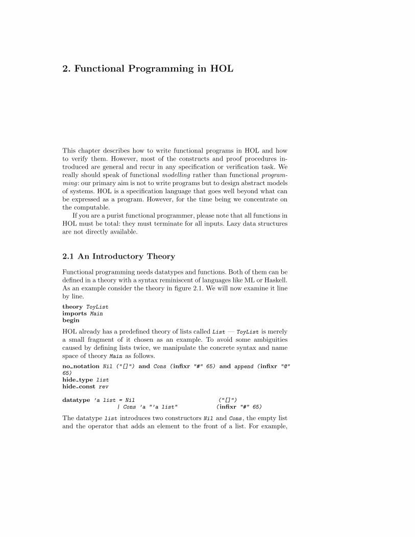
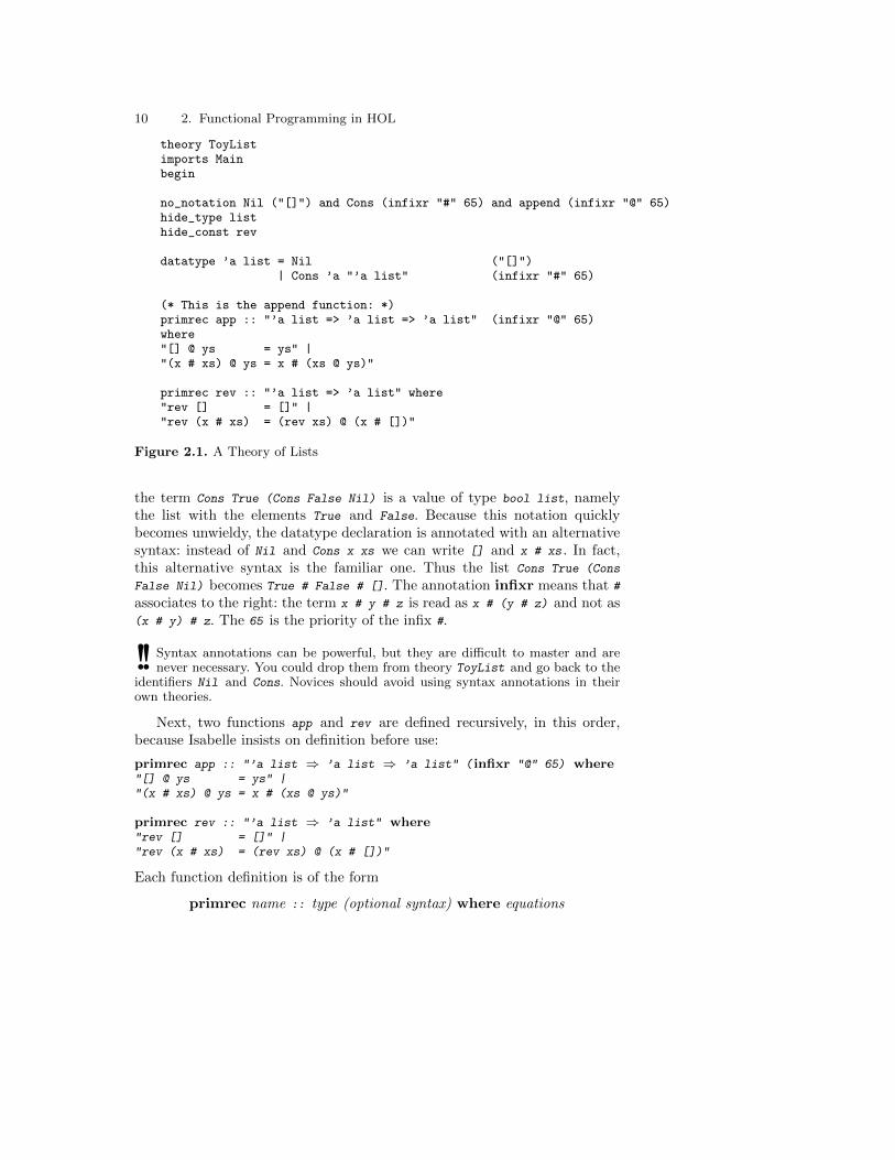
Functional programming needs datatypes and functions. Both of them can bedefined in a theory with a syntax reminiscent of languages like ML or Haskell.As an example consider the theory in figure 2.1. We will now examine it lineby line.
theory ToyListimports Mainbegin
HOL already has a predefined theory of lists called List — ToyList is merelya small fragment of it chosen as an example. To avoid some ambiguitiescaused by defining lists twice, we manipulate the concrete syntax and namespace of theory Main as follows.
no notation Nil ("[]") and Cons ( infixr "#" 65) and append ( infixr "@"65)hide type listhide const rev
datatype ’a list = Nil ("[]")| Cons ’a "’a list" ( infixr "#" 65)
The datatype list introduces two constructors Nil and Cons , the empty listand the operator that adds an element to the front of a list. For example,
10 2. Functional Programming in HOL
theory ToyListimports Mainbegin
no_notation Nil ("[]") and Cons (infixr "#" 65) and append (infixr "@" 65)hide_type listhide_const rev
datatype ’a list = Nil ("[]")| Cons ’a "’a list" (infixr "#" 65)
(* This is the append function: *)primrec app :: "’a list => ’a list => ’a list" (infixr "@" 65)where"[] @ ys = ys" |"(x # xs) @ ys = x # (xs @ ys)"
primrec rev :: "’a list => ’a list" where"rev [] = []" |"rev (x # xs) = (rev xs) @ (x # [])"
Figure 2.1. A Theory of Lists
the term Cons True (Cons False Nil) is a value of type bool list, namelythe list with the elements True and False. Because this notation quicklybecomes unwieldy, the datatype declaration is annotated with an alternativesyntax: instead of Nil and Cons x xs we can write [] and x # xs . In fact,this alternative syntax is the familiar one. Thus the list Cons True (Cons
False Nil) becomes True # False # []. The annotation infixr means that #
associates to the right: the term x # y # z is read as x # (y # z) and not as(x # y) # z. The 65 is the priority of the infix #.
!! Syntax annotations can be powerful, but they are difficult to master and arenever necessary. You could drop them from theory ToyList and go back to the
identifiers Nil and Cons. Novices should avoid using syntax annotations in theirown theories.
Next, two functions app and rev are defined recursively, in this order,because Isabelle insists on definition before use:
primrec app :: "’a list ⇒ ’a list ⇒ ’a list" ( infixr "@" 65) where"[] @ ys = ys" |"(x # xs) @ ys = x # (xs @ ys)"
primrec rev :: "’a list ⇒ ’a list" where"rev [] = []" |"rev (x # xs) = (rev xs) @ (x # [])"
Each function definition is of the form
primrec name :: type (optional syntax) where equations
2.2 Evaluation 11
The equations must be separated by |. Function app is annotated with con-crete syntax. Instead of the prefix syntax app xs ys the infix xs @ ys becomesthe preferred form.
The equations for app and rev hardly need comments: app appends twolists and rev reverses a list. The keyword primrec indicates that the recur-sion is of a particularly primitive kind where each recursive call peels off adatatype constructor from one of the arguments. Thus the recursion alwaysterminates, i.e. the function is total.
The termination requirement is absolutely essential in HOL, a logic oftotal functions. If we were to drop it, inconsistencies would quickly arise: the“definition” f (n) = f (n) + 1 immediately leads to 0 = 1 by subtracting f (n)on both sides.
!! As we have indicated, the requirement for total functions is an essential char-acteristic of HOL. It is only because of totality that reasoning in HOL is com-
paratively easy. More generally, the philosophy in HOL is to refrain from assertingarbitrary axioms (such as function definitions whose totality has not been proved)because they quickly lead to inconsistencies. Instead, fixed constructs for introduc-ing types and functions are offered (such as datatype and primrec) which areguaranteed to preserve consistency.
A remark about syntax. The textual definition of a theory follows a fixedsyntax with keywords like datatype and end. Embedded in this syntax arethe types and formulae of HOL, whose syntax is extensible (see Sect. 4.1), e.g.by new user-defined infix operators. To distinguish the two levels, everythingHOL-specific (terms and types) should be enclosed in ". . . ". To lessen thisburden, quotation marks around a single identifier can be dropped, unless theidentifier happens to be a keyword, for example "end". When Isabelle printsa syntax error message, it refers to the HOL syntax as the inner syntax andthe enclosing theory language as the outer syntax.
Comments must be in enclosed in (* and *).
2.2 Evaluation
Assuming you have processed the declarations and definitions of ToyList
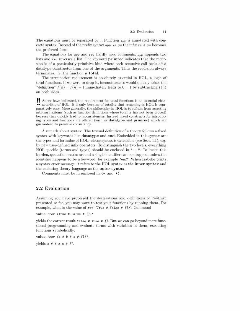
presented so far, you may want to test your functions by running them. Forexample, what is the value of rev (True # False # [])? Command
value "rev (True # False # [])"
yields the correct result False # True # []. But we can go beyond mere func-tional programming and evaluate terms with variables in them, executingfunctions symbolically:
value "rev (a # b # c # [])"
yields c # b # a # [].
12 2. Functional Programming in HOL
2.3 An Introductory Proof
Having convinced ourselves (as well as one can by testing) that our definitionscapture our intentions, we are ready to prove a few simple theorems. Thiswill illustrate not just the basic proof commands but also the typical proofprocess.
Main Goal. Our goal is to show that reversing a list twice produces theoriginal list.
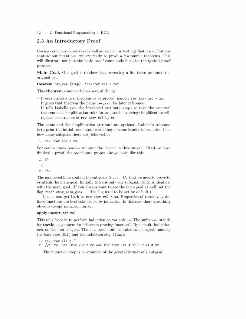
theorem rev_rev [simp]: "rev(rev xs) = xs"
This theorem command does several things:
– It establishes a new theorem to be proved, namely rev (rev xs) = xs.– It gives that theorem the name rev_rev, for later reference.– It tells Isabelle (via the bracketed attribute simp) to take the eventual
theorem as a simplification rule: future proofs involving simplification willreplace occurrences of rev (rev xs) by xs.
The name and the simplification attribute are optional. Isabelle’s responseis to print the initial proof state consisting of some header information (likehow many subgoals there are) followed by
1. rev (rev xs) = xs
For compactness reasons we omit the header in this tutorial. Until we havefinished a proof, the proof state proper always looks like this:
1. G1
...n. Gn
The numbered lines contain the subgoals G1, . . . , Gn that we need to prove toestablish the main goal. Initially there is only one subgoal, which is identicalwith the main goal. (If you always want to see the main goal as well, set theflag Proof.show_main_goal — this flag used to be set by default.)
Let us now get back to rev (rev xs) = xs. Properties of recursively de-fined functions are best established by induction. In this case there is nothingobvious except induction on xs :
apply(induct_tac xs)
This tells Isabelle to perform induction on variable xs. The suffix tac standsfor tactic, a synonym for “theorem proving function”. By default, inductionacts on the first subgoal. The new proof state contains two subgoals, namelythe base case (Nil) and the induction step (Cons):
1. rev (rev []) = []2.
∧x1 x2. rev (rev x2) = x2 =⇒ rev (rev (x1 # x2)) = x1 # x2
The induction step is an example of the general format of a subgoal:
2.3 An Introductory Proof 13
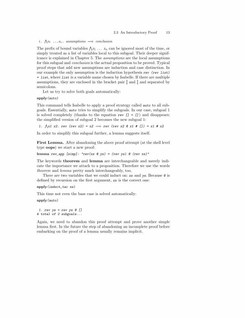
i.∧
x1 ...xn. assumptions =⇒ conclusion
The prefix of bound variables∧
x1 . . . xn can be ignored most of the time, orsimply treated as a list of variables local to this subgoal. Their deeper signif-icance is explained in Chapter 5. The assumptions are the local assumptionsfor this subgoal and conclusion is the actual proposition to be proved. Typicalproof steps that add new assumptions are induction and case distinction. Inour example the only assumption is the induction hypothesis rev (rev list)
= list, where list is a variable name chosen by Isabelle. If there are multipleassumptions, they are enclosed in the bracket pair [[ and ]] and separated bysemicolons.
Let us try to solve both goals automatically:
apply(auto)
This command tells Isabelle to apply a proof strategy called auto to all sub-goals. Essentially, auto tries to simplify the subgoals. In our case, subgoal 1is solved completely (thanks to the equation rev [] = []) and disappears;the simplified version of subgoal 2 becomes the new subgoal 1:
1.∧x1 x2. rev (rev x2) = x2 =⇒ rev (rev x2 @ x1 # []) = x1 # x2
In order to simplify this subgoal further, a lemma suggests itself.
First Lemma. After abandoning the above proof attempt (at the shell leveltype oops) we start a new proof:
lemma rev_app [simp]: "rev(xs @ ys) = (rev ys) @ (rev xs)"
The keywords theorem and lemma are interchangeable and merely indi-cate the importance we attach to a proposition. Therefore we use the wordstheorem and lemma pretty much interchangeably, too.
There are two variables that we could induct on: xs and ys. Because @ isdefined by recursion on the first argument, xs is the correct one:
apply(induct_tac xs)
This time not even the base case is solved automatically:
apply(auto)
1. rev ys = rev ys @ []A total of 2 subgoals...
Again, we need to abandon this proof attempt and prove another simplelemma first. In the future the step of abandoning an incomplete proof beforeembarking on the proof of a lemma usually remains implicit.
14 2. Functional Programming in HOL
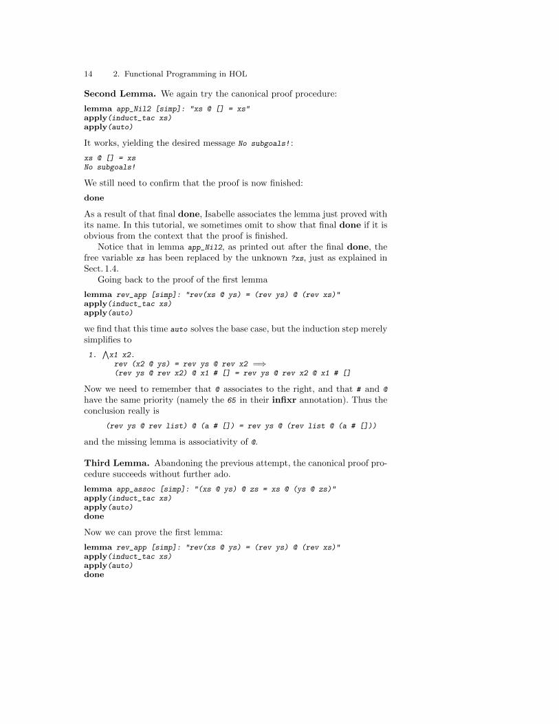
Second Lemma. We again try the canonical proof procedure:
lemma app_Nil2 [simp]: "xs @ [] = xs"apply(induct_tac xs)apply(auto)
It works, yielding the desired message No subgoals! :
xs @ [] = xsNo subgoals!
We still need to confirm that the proof is now finished:
done
As a result of that final done, Isabelle associates the lemma just proved withits name. In this tutorial, we sometimes omit to show that final done if it isobvious from the context that the proof is finished.
Notice that in lemma app_Nil2, as printed out after the final done, thefree variable xs has been replaced by the unknown ?xs, just as explained inSect. 1.4.
Going back to the proof of the first lemma
lemma rev_app [simp]: "rev(xs @ ys) = (rev ys) @ (rev xs)"apply(induct_tac xs)apply(auto)
we find that this time auto solves the base case, but the induction step merelysimplifies to
1.∧x1 x2.rev (x2 @ ys) = rev ys @ rev x2 =⇒(rev ys @ rev x2) @ x1 # [] = rev ys @ rev x2 @ x1 # []
Now we need to remember that @ associates to the right, and that # and @
have the same priority (namely the 65 in their infixr annotation). Thus theconclusion really is
(rev ys @ rev list) @ (a # []) = rev ys @ (rev list @ (a # []))
and the missing lemma is associativity of @.
Third Lemma. Abandoning the previous attempt, the canonical proof pro-cedure succeeds without further ado.
lemma app_assoc [simp]: "(xs @ ys) @ zs = xs @ (ys @ zs)"apply(induct_tac xs)apply(auto)done
Now we can prove the first lemma:
lemma rev_app [simp]: "rev(xs @ ys) = (rev ys) @ (rev xs)"apply(induct_tac xs)apply(auto)done
2.3 An Introductory Proof 15
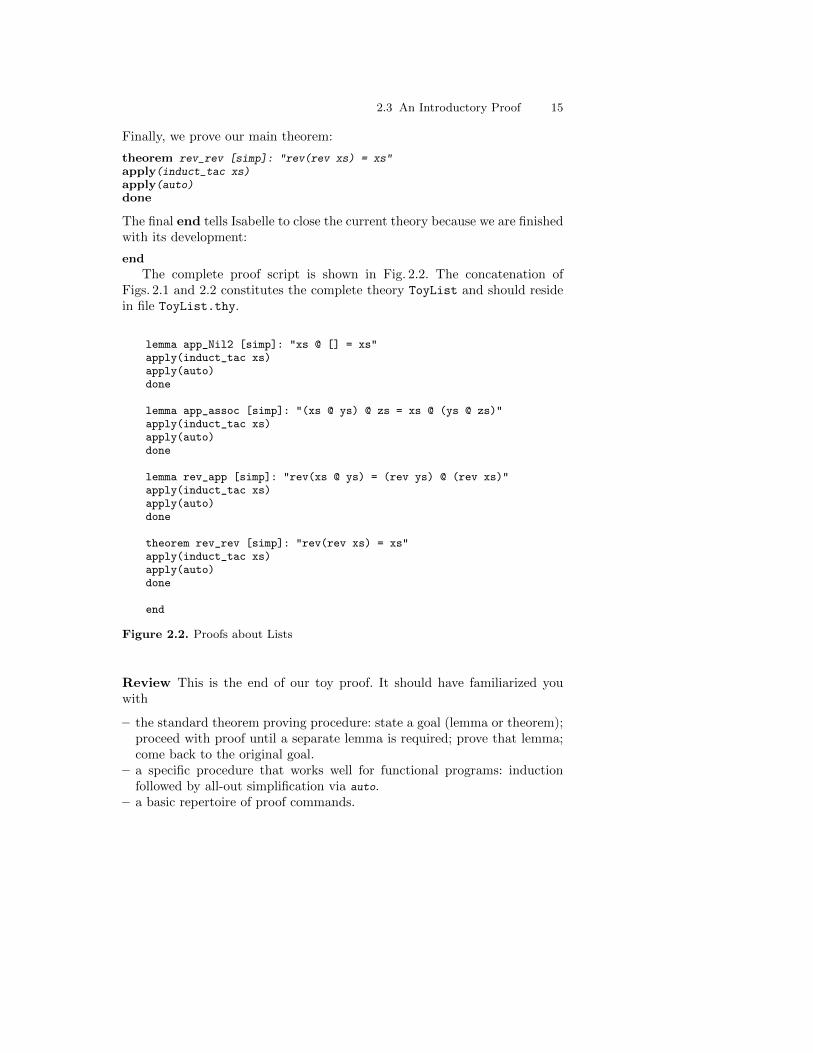
Finally, we prove our main theorem:
theorem rev_rev [simp]: "rev(rev xs) = xs"apply(induct_tac xs)apply(auto)done
The final end tells Isabelle to close the current theory because we are finishedwith its development:
end
The complete proof script is shown in Fig. 2.2. The concatenation ofFigs. 2.1 and 2.2 constitutes the complete theory ToyList and should residein file ToyList.thy.
lemma app_Nil2 [simp]: "xs @ [] = xs"apply(induct_tac xs)apply(auto)done
lemma app_assoc [simp]: "(xs @ ys) @ zs = xs @ (ys @ zs)"apply(induct_tac xs)apply(auto)done
lemma rev_app [simp]: "rev(xs @ ys) = (rev ys) @ (rev xs)"apply(induct_tac xs)apply(auto)done
theorem rev_rev [simp]: "rev(rev xs) = xs"apply(induct_tac xs)apply(auto)done
end
Figure 2.2. Proofs about Lists
Review This is the end of our toy proof. It should have familiarized youwith
– the standard theorem proving procedure: state a goal (lemma or theorem);proceed with proof until a separate lemma is required; prove that lemma;come back to the original goal.
– a specific procedure that works well for functional programs: inductionfollowed by all-out simplification via auto.
– a basic repertoire of proof commands.
16 2. Functional Programming in HOL
!! It is tempting to think that all lemmas should have the simp attribute justbecause this was the case in the example above. However, in that example all
lemmas were equations, and the right-hand side was simpler than the left-handside — an ideal situation for simplification purposes. Unless this is clearly the case,novices should refrain from awarding a lemma the simp attribute, which has aglobal effect. Instead, lemmas can be applied locally where they are needed, whichis discussed in the following chapter.
2.4 Some Helpful Commands
This section discusses a few basic commands for manipulating the proof stateand can be skipped by casual readers.
There are two kinds of commands used during a proof: the actual proofcommands and auxiliary commands for examining the proof state and con-trolling the display. Simple proof commands are of the form apply(method),where method is typically induct_tac or auto. All such theorem proving oper-ations are referred to as methods, and further ones are introduced through-out the tutorial. Unless stated otherwise, you may assume that a methodattacks merely the first subgoal. An exception is auto, which tries to solve allsubgoals.
The most useful auxiliary commands are as follows:
Modifying the order of subgoals: defer moves the first subgoal to the endand prefer n moves subgoal n to the front.
Printing theorems: thm name1 . . . namen prints the named theorems.Reading terms and types: term string reads, type-checks and prints the
given string as a term in the current context; the inferred type is outputas well. typ string reads and prints the given string as a type in thecurrent context.
Further commands are found in the Isabelle/Isar Reference Manual [38].
Clicking on the State button redisplays the current proof state. This is helpfulin case commands like thm have overwritten it.
We now examine Isabelle’s functional programming constructs systemat-ically, starting with inductive datatypes.
2.5 Datatypes
Inductive datatypes are part of almost every non-trivial application of HOL.First we take another look at an important example, the datatype of lists,before we turn to datatypes in general. The section closes with a case study.
2.5 Datatypes 17
2.5.1 Lists
Lists are one of the essential datatypes in computing. We expect that you arealready familiar with their basic operations. Theory ToyList is only a smallfragment of HOL’s predefined theory List1. The latter contains many furtheroperations. For example, the functions hd (“head”) and tl (“tail”) returnthe first element and the remainder of a list. (However, pattern matching isusually preferable to hd and tl.) Also available are higher-order functions likemap and filter. Theory List also contains more syntactic sugar: [x1, . . . ,xn]abbreviates x1# . . . #xn#[]. In the rest of the tutorial we always use HOL’spredefined lists by building on theory Main.
!! Looking ahead to sets and quanifiers in Part II: The best way to express thatsome element x is in a list xs is x ∈ set xs, where set is a function that turns
a list into the set of its elements. By the same device you can also write boundedquantifiers like ∀x ∈ set xs or embed lists in other set expressions.
2.5.2 The General Format
The general HOL datatype definition is of the form
datatype (α1, . . . , αn) t = C1 τ11 . . . τ1k1 | . . . | Cm τm1 . . . τmkm
where αi are distinct type variables (the parameters), Ci are distinct con-structor names and τij are types; it is customary to capitalize the first letterin constructor names. There are a number of restrictions (such as that thetype should not be empty) detailed elsewhere [26]. Isabelle notifies you if youviolate them.
Laws about datatypes, such as [] 6= x#xs and (x#xs = y#ys) = (x=y
∧ xs=ys), are used automatically during proofs by simplification. The sameis true for the equations in primitive recursive function definitions.
Every2 datatype t comes equipped with a size function from t into thenatural numbers (see Sect. 2.6.1 below). For lists, size is just the length, i.e.size [] = 0 and size(x # xs) = size xs + 1. In general, size returns
– zero for all constructors that do not have an argument of type t ,– one plus the sum of the sizes of all arguments of type t , for all other
constructors.
Note that because size is defined on every datatype, it is overloaded; on listssize is also called length , which is not overloaded. Isabelle will always showsize on lists as length.
1 https://isabelle.in.tum.de/library/HOL/List.html2 Except for advanced datatypes where the recursion involves “⇒” as in Sect. 3.4.3.
18 2. Functional Programming in HOL
2.5.3 Primitive Recursion
Functions on datatypes are usually defined by recursion. In fact, most ofthe time they are defined by what is called primitive recursion over somedatatype t . This means that the recursion equations must be of the form
f x1 . . . (C y1 . . . yk ) . . . xn = r
such that C is a constructor of t and all recursive calls of f in r are of theform f . . . yi . . . for some i . Thus Isabelle immediately sees that f terminatesbecause one (fixed!) argument becomes smaller with every recursive call.There must be at most one equation for each constructor. Their order isimmaterial. A more general method for defining total recursive functions isintroduced in Sect. 3.5.
Exercise 2.5.1 Define the datatype of binary trees:
datatype ’a tree = Tip | Node "’a tree" ’a "’a tree"
Define a function mirror that mirrors a binary tree by swapping subtreesrecursively. Prove
lemma mirror_mirror: "mirror(mirror t) = t"
Define a function flatten that flattens a tree into a list by traversing it ininfix order. Prove
lemma "flatten(mirror t) = rev(flatten t)"
2.5.4 Case Expressions
HOL also features case -expressions for analyzing elements of a datatype. Forexample,
case xs of [] ⇒ [] | y # ys ⇒ y
evaluates to [] if xs is [] and to y if xs is y # ys. (Since the result in bothbranches must be of the same type, it follows that y is of type ’a list andhence that xs is of type ’a list list.)
In general, case expressions are of the form
case e of pattern1 ⇒ e1 | . . . | patternm ⇒ em
Like in functional programming, patterns are expressions consisting of data-type constructors (e.g. [] and #) and variables, including the wildcard “_”.Not all cases need to be covered and the order of cases matters. However,one is well-advised not to wallow in complex patterns because complex casedistinctions tend to induce complex proofs.
2.5 Datatypes 19
!! Internally Isabelle only knows about exhaustive case expressions with non-nested patterns: patterni must be of the form Ci xi1 . . . xiki and C1, . . . ,Cm
must be exactly the constructors of the type of e. More complex case expressions areautomatically translated into the simpler form upon parsing but are not translatedback for printing. This may lead to surprising output.
!! Like if, case -expressions may need to be enclosed in parentheses to indicatetheir scope.
2.5.5 Structural Induction and Case Distinction
Induction is invoked by induct_tac , as we have seen above; it works for anydatatype. In some cases, induction is overkill and a case distinction over allconstructors of the datatype suffices. This is performed by case_tac . Here isa trivial example:
lemma "(case xs of [] ⇒ [] | y#ys ⇒ xs) = xs"apply(case_tac xs)
results in the proof state
1. xs = [] =⇒ (case xs of [] ⇒ [] | y # ys ⇒ xs) = xs2.
∧a list.xs = a # list =⇒ (case xs of [] ⇒ [] | y # ys ⇒ xs) = xs
which is solved automatically:
apply(auto)
Note that we do not need to give a lemma a name if we do not intendto refer to it explicitly in the future. Other basic laws about a datatypeare applied automatically during simplification, so no special methods areprovided for them.
!! Induction is only allowed on free (or∧
-bound) variables that should not occuramong the assumptions of the subgoal; see Sect. 9.2.1 for details. Case distinc-
tion (case_tac) works for arbitrary terms, which need to be quoted if they arenon-atomic. However, apart from
∧-bound variables, the terms must not contain
variables that are bound outside. For example, given the goal ∀ xs. xs = [] ∨(∃ y ys. xs = y # ys), case_tac xs will not work as expected because Isabelleinterprets the xs as a new free variable distinct from the bound xs in the goal.
2.5.6 Case Study: Boolean Expressions
The aim of this case study is twofold: it shows how to model boolean expres-sions and some algorithms for manipulating them, and it demonstrates theconstructs introduced above.
20 2. Functional Programming in HOL
Modelling Boolean Expressions. We want to represent boolean expres-sions built up from variables and constants by negation and conjunction. Thefollowing datatype serves exactly that purpose:
datatype boolex = Const bool | Var nat | Neg boolex| And boolex boolex
The two constants are represented by Const True and Const False. Variablesare represented by terms of the form Var n, where n is a natural number(type nat). For example, the formula P0 ∧ ¬P1 is represented by the termAnd (Var 0) (Neg (Var 1)).
The Value of a Boolean Expression. The value of a boolean expressiondepends on the value of its variables. Hence the function value takes an addi-tional parameter, an environment of type nat ⇒ bool, which maps variablesto their values:
primrec "value" :: "boolex ⇒ (nat ⇒ bool) ⇒ bool" where"value (Const b) env = b" |"value (Var x) env = env x" |"value (Neg b) env = (¬ value b env)" |"value (And b c) env = (value b env ∧ value c env)"
If-Expressions. An alternative and often more efficient (because in a cer-tain sense canonical) representation are so-called If-expressions built up fromconstants (CIF), variables (VIF) and conditionals (IF):
datatype ifex = CIF bool | VIF nat | IF ifex ifex ifex
The evaluation of If-expressions proceeds as for boolex :
primrec valif :: "ifex ⇒ (nat ⇒ bool) ⇒ bool" where"valif (CIF b) env = b" |"valif (VIF x) env = env x" |"valif (IF b t e) env = (if valif b env then valif t env
else valif e env)"
Converting Boolean and If-Expressions. The type boolex is close tothe customary representation of logical formulae, whereas ifex is designedfor efficiency. It is easy to translate from boolex into ifex :
primrec bool2if :: "boolex ⇒ ifex" where"bool2if (Const b) = CIF b" |"bool2if (Var x) = VIF x" |"bool2if (Neg b) = IF (bool2if b) (CIF False) (CIF True)" |"bool2if (And b c) = IF (bool2if b) (bool2if c) (CIF False)"
At last, we have something we can verify: that bool2if preserves the valueof its argument:
lemma "valif (bool2if b) env = value b env"
The proof is canonical:
apply(induct_tac b)
2.5 Datatypes 21
apply(auto)done
In fact, all proofs in this case study look exactly like this. Hence we do notshow them below.
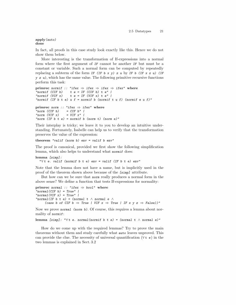
More interesting is the transformation of If-expressions into a normalform where the first argument of IF cannot be another IF but must be aconstant or variable. Such a normal form can be computed by repeatedlyreplacing a subterm of the form IF (IF b x y) z u by IF b (IF x z u) (IF
y z u), which has the same value. The following primitive recursive functionsperform this task:
primrec normif :: "ifex ⇒ ifex ⇒ ifex ⇒ ifex" where"normif (CIF b) t e = IF (CIF b) t e" |"normif (VIF x) t e = IF (VIF x) t e" |"normif (IF b t e) u f = normif b (normif t u f) (normif e u f)"
primrec norm :: "ifex ⇒ ifex" where"norm (CIF b) = CIF b" |"norm (VIF x) = VIF x" |"norm (IF b t e) = normif b (norm t) (norm e)"
Their interplay is tricky; we leave it to you to develop an intuitive under-standing. Fortunately, Isabelle can help us to verify that the transformationpreserves the value of the expression:
theorem "valif (norm b) env = valif b env"
The proof is canonical, provided we first show the following simplificationlemma, which also helps to understand what normif does:
lemma [simp]:"∀ t e. valif (normif b t e) env = valif (IF b t e) env"
Note that the lemma does not have a name, but is implicitly used in theproof of the theorem shown above because of the [simp] attribute.
But how can we be sure that norm really produces a normal form in theabove sense? We define a function that tests If-expressions for normality:
primrec normal :: "ifex ⇒ bool" where"normal(CIF b) = True" |"normal(VIF x) = True" |"normal(IF b t e) = (normal t ∧ normal e ∧
(case b of CIF b ⇒ True | VIF x ⇒ True | IF x y z ⇒ False))"
Now we prove normal (norm b). Of course, this requires a lemma about nor-mality of normif :
lemma [simp]: "∀ t e. normal(normif b t e) = (normal t ∧ normal e)"
How do we come up with the required lemmas? Try to prove the maintheorems without them and study carefully what auto leaves unproved. Thiscan provide the clue. The necessity of universal quantification (∀ t e) in thetwo lemmas is explained in Sect. 3.2
22 2. Functional Programming in HOL
Exercise 2.5.2 We strengthen the definition of a normal If-expression asfollows: the first argument of all IFs must be a variable. Adapt the abovedevelopment to this changed requirement. (Hint: you may need to formulatesome of the goals as implications (−→) rather than equalities (=).)
2.6 Some Basic Types
This section introduces the types of natural numbers and ordered pairs. Alsodescribed is type option, which is useful for modelling exceptional cases.
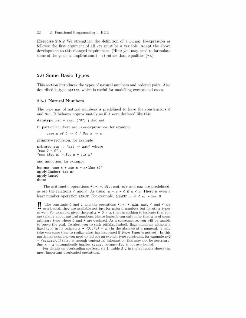
2.6.1 Natural Numbers
The type nat of natural numbers is predefined to have the constructors 0
and Suc . It behaves approximately as if it were declared like this:
datatype nat = zero ("0") | Suc nat
In particular, there are case -expressions, for example
case n of 0 ⇒ 0 | Suc m ⇒ m
primitive recursion, for example
primrec sum :: "nat ⇒ nat" where"sum 0 = 0" |"sum (Suc n) = Suc n + sum n"
and induction, for example
lemma "sum n + sum n = n*(Suc n)"apply(induct_tac n)apply(auto)done
The arithmetic operations + , - , * , div , mod , min and max are predefined,as are the relations ≤ and < . As usual, m - n = 0 if m < n. There is even aleast number operation LEAST . For example, (LEAST n. 0 < n) = Suc 0.
!! The constants 0 and 1 and the operations + , - , * , min , max , ≤ and < areoverloaded: they are available not just for natural numbers but for other types
as well. For example, given the goal x + 0 = x, there is nothing to indicate that youare talking about natural numbers. Hence Isabelle can only infer that x is of somearbitrary type where 0 and + are declared. As a consequence, you will be unableto prove the goal. To alert you to such pitfalls, Isabelle flags numerals without afixed type in its output: x + (0::’a) = x. (In the absence of a numeral, it maytake you some time to realize what has happened if Show Types is not set). In thisparticular example, you need to include an explicit type constraint, for example x+0= (x::nat). If there is enough contextual information this may not be necessary:Suc x = x automatically implies x::nat because Suc is not overloaded.
For details on overloading see Sect. 8.3.1. Table A.2 in the appendix shows themost important overloaded operations.
2.6 Some Basic Types 23
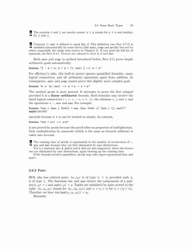
!! The symbols > and ≥ are merely syntax: x > y stands for y < x and similaryfor ≥ and ≤.
!! Constant 1::nat is defined to equal Suc 0. This definition (see Sect. 2.7.2) isunfolded automatically by some tactics (like auto, simp and arith) but not by
others (especially the single step tactics in Chapter 5). If you need the full set ofnumerals, see Sect. 8.4.1. Novices are advised to stick to 0 and Suc.
Both auto and simp (a method introduced below, Sect. 3.1) prove simplearithmetic goals automatically:
lemma " [[ ¬ m < n; m < n + (1::nat) ]] =⇒ m = n"
For efficiency’s sake, this built-in prover ignores quantified formulae, manylogical connectives, and all arithmetic operations apart from addition. Inconsequence, auto and simp cannot prove this slightly more complex goal:
lemma "m 6= (n::nat) =⇒ m < n ∨ n < m"
The method arith is more general. It attempts to prove the first subgoalprovided it is a linear arithmetic formula. Such formulas may involve theusual logical connectives (¬, ∧, ∨, −→, =, ∀ , ∃ ), the relations =, ≤ and <, andthe operations +, -, min and max. For example,
lemma "min i (max j (k*k)) = max (min (k*k) i) (min i (j::nat))"apply(arith)
succeeds because k * k can be treated as atomic. In contrast,
lemma "n*n = n+1 =⇒ n=0"
is not proved by arith because the proof relies on properties of multiplication.Only multiplication by numerals (which is the same as iterated addition) istaken into account.
!! The running time of arith is exponential in the number of occurrences of - ,min and max because they are first eliminated by case distinctions.If k is a numeral, div k, mod k and k dvd are also supported, where the former
two are eliminated by case distinctions, again blowing up the running time.If the formula involves quantifiers, arith may take super-exponential time and
space.
2.6.2 Pairs
HOL also has ordered pairs: (a1,a2) is of type τ1 × τ2 provided each ai
is of type τi . The functions fst and snd extract the components of a pair:fst(x,y) = x and snd(x,y) = y. Tuples are simulated by pairs nested to theright: (a1,a2,a3) stands for (a1,(a2,a3)) and τ1 × τ2 × τ3 for τ1 × (τ2 × τ3).Therefore we have fst(snd(a1,a2,a3)) = a2.
Remarks:
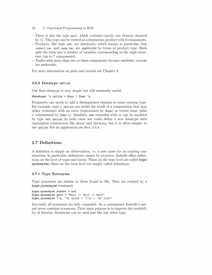
24 2. Functional Programming in HOL
– There is also the type unit , which contains exactly one element denotedby () . This type can be viewed as a degenerate product with 0 components.
– Products, like type nat, are datatypes, which means in particular thatinduct_tac and case_tac are applicable to terms of product type. Bothsplit the term into a number of variables corresponding to the tuple struc-ture (up to 7 components).
– Tuples with more than two or three components become unwieldy; recordsare preferable.
For more information on pairs and records see Chapter 8.
2.6.3 Datatype option
Our final datatype is very simple but still eminently useful:
datatype ’a option = None | Some ’a
Frequently one needs to add a distinguished element to some existing type.For example, type t option can model the result of a computation that mayeither terminate with an error (represented by None) or return some valuev (represented by Some v). Similarly, nat extended with ∞ can be modeledby type nat option. In both cases one could define a new datatype withcustomized constructors like Error and Infinity, but it is often simpler touse option. For an application see Sect. 3.4.4.
2.7 Definitions
A definition is simply an abbreviation, i.e. a new name for an existing con-struction. In particular, definitions cannot be recursive. Isabelle offers defini-tions on the level of types and terms. Those on the type level are called typesynonyms; those on the term level are simply called definitions.
2.7.1 Type Synonyms
Type synonyms are similar to those found in ML. They are created by atype synonym command:
type synonym number = nattype synonym gate = "bool ⇒ bool ⇒ bool"type synonym (’a, ’b) alist = "(’a × ’b) list"
Internally all synonyms are fully expanded. As a consequence Isabelle’s out-put never contains synonyms. Their main purpose is to improve the readabil-ity of theories. Synonyms can be used just like any other type.
2.8 The Definitional Approach 25
2.7.2 Constant Definitions
Nonrecursive definitions can be made with the definition command, forexample nand and xor gates (based on type gate above):
definition nand :: gate where "nand A B ≡ ¬(A ∧ B)"definition xor :: gate where "xor A B ≡ A ∧ ¬B ∨ ¬A ∧ B"
The symbol ≡ is a special form of equality that must be used in constantdefinitions. Pattern-matching is not allowed: each definition must be of theform f x1 . . . xn ≡ t . Section 3.1.6 explains how definitions are used in proofs.The default name of each definition is f _def, where f is the name of thedefined constant.
!! A common mistake when writing definitions is to introduce extra free variableson the right-hand side. Consider the following, flawed definition (where dvd
means “divides”):
"prime p ≡ 1 < p ∧ (m dvd p −→ m = 1 ∨ m = p)"
Isabelle rejects this “definition” because of the extra m on the right-hand side, whichwould introduce an inconsistency (why?). The correct version is
"prime p ≡ 1 < p ∧ (∀ m. m dvd p −→ m = 1 ∨ m = p)"
2.8 The Definitional Approach
As we pointed out at the beginning of the chapter, asserting arbitrary ax-ioms such as f (n) = f (n) + 1 can easily lead to contradictions. In order toavoid this danger, we advocate the definitional rather than the axiomatic ap-proach: introduce new concepts by definitions. However, Isabelle/HOL seemsto support many richer definitional constructs, such as primrec. The pointis that Isabelle reduces such constructs to first principles. For example, eachprimrec function definition is turned into a proper (nonrecursive!) definitionfrom which the user-supplied recursion equations are automatically proved.This process is hidden from the user, who does not have to understand thedetails. Other commands described later, like fun and inductive, work sim-ilarly. This strict adherence to the definitional approach reduces the risk ofsoundness errors.

3. More Functional Programming
The purpose of this chapter is to deepen your understanding of the con-cepts encountered so far and to introduce advanced forms of datatypes andrecursive functions. The first two sections give a structured presentation oftheorem proving by simplification (Sect. 3.1) and discuss important heuris-tics for induction (Sect. 3.2). You can skip them if you are not planning toperform proofs yourself. We then present a case study: a compiler for ex-pressions (Sect. 3.3). Advanced datatypes, including those involving functionspaces, are covered in Sect. 3.4; it closes with another case study, search trees(“tries”). Finally we introduce fun, a general form of recursive function def-inition that goes well beyond primrec (Sect. 3.5).
3.1 Simplification
So far we have proved our theorems by auto, which simplifies all subgoals.In fact, auto can do much more than that. To go beyond toy examples, youneed to understand the ingredients of auto. This section covers the methodthat auto always applies first, simplification.
Simplification is one of the central theorem proving tools in Isabelle andmany other systems. The tool itself is called the simplifier. This sectionintroduces the many features of the simplifier and is required reading if youintend to perform proofs. Later on, Sect. 9.1 explains some more advancedfeatures and a little bit of how the simplifier works. The serious student shouldread that section as well, in particular to understand why the simplifier didsomething unexpected.
3.1.1 What is Simplification?
In its most basic form, simplification means repeated application of equationsfrom left to right. For example, taking the rules for @ and applying them tothe term [0,1] @ [] results in a sequence of simplification steps:
(0#1#[]) @ [] ; 0#((1#[]) @ []) ; 0#(1#([] @ [])) ; 0#1#[]
This is also known as term rewriting and the equations are referred to asrewrite rules. “Rewriting” is more honest than “simplification” because theterms do not necessarily become simpler in the process.
28 3. More Functional Programming
The simplifier proves arithmetic goals as described in Sect. 2.6.1 above.Arithmetic expressions are simplified using built-in procedures that go be-yond mere rewrite rules. New simplification procedures can be coded andinstalled, but they are definitely not a matter for this tutorial.
3.1.2 Simplification Rules
To facilitate simplification, the attribute [simp] declares theorems to be sim-plification rules, which the simplifier will use automatically. In addition,datatype and primrec declarations (and a few others) implicitly declaresome simplification rules. Explicit definitions are not declared as simplifica-tion rules automatically!
Nearly any theorem can become a simplification rule. The simplifier willtry to transform it into an equation. For example, the theorem ¬ P is turnedinto P = False. The details are explained in Sect. 9.1.2.
The simplification attribute of theorems can be turned on and off:
declare theorem-name[simp]declare theorem-name[simp del]
Only equations that really simplify, like rev (rev xs) = xs and xs @ [] = xs,should be declared as default simplification rules. More specific ones shouldonly be used selectively and should not be made default. Distributivity laws,for example, alter the structure of terms and can produce an exponentialblow-up instead of simplification. A default simplification rule may need tobe disabled in certain proofs. Frequent changes in the simplification status ofa theorem may indicate an unwise use of defaults.
!! Simplification can run forever, for example if both f (x ) = g(x ) and g(x ) = f (x )are simplification rules. It is the user’s responsibility not to include simplification
rules that can lead to nontermination, either on their own or in combination withother simplification rules.
!! It is inadvisable to toggle the simplification attribute of a theorem from a parenttheory A in a child theory B for good. The reason is that if some theory C
is based both on B and (via a different path) on A, it is not defined what thesimplification attribute of that theorem will be in C : it could be either.
3.1.3 The simp Method
The general format of the simplification method is
simp list of modifiers
where the list of modifiers fine tunes the behaviour and may be empty. Spe-cific modifiers are discussed below. Most if not all of the proofs seen so far
3.1 Simplification 29
could have been performed with simp instead of auto, except that simp at-tacks only the first subgoal and may thus need to be repeated — use simp_all
to simplify all subgoals. If nothing changes, simp fails.
3.1.4 Adding and Deleting Simplification Rules
If a certain theorem is merely needed in a few proofs by simplification, we donot need to make it a global simplification rule. Instead we can modify theset of simplification rules used in a simplification step by adding rules to itand/or deleting rules from it. The two modifiers for this are
add: list of theorem namesdel: list of theorem names
Or you can use a specific list of theorems and omit all others:
only: list of theorem names
In this example, we invoke the simplifier, adding two distributive laws:
apply(simp add: mod_mult_distrib add_mult_distrib)
3.1.5 Assumptions
By default, assumptions are part of the simplification process: they are usedas simplification rules and are simplified themselves. For example:
lemma " [[ xs @ zs = ys @ xs; [] @ xs = [] @ [] ]] =⇒ ys = zs"apply simpdone
The second assumption simplifies to xs = [], which in turn simplifies the firstassumption to zs = ys, thus reducing the conclusion to ys = ys and henceto True.
In some cases, using the assumptions can lead to nontermination:
lemma "∀ x. f x = g (f (g x)) =⇒ f [] = f [] @ []"
An unmodified application of simp loops. The culprit is the simplification rulef x = g (f (g x)), which is extracted from the assumption. (Isabelle noticescertain simple forms of nontermination but not this one.) The problem canbe circumvented by telling the simplifier to ignore the assumptions:
apply(simp (no_asm))done
Three modifiers influence the treatment of assumptions:
(no_asm) means that assumptions are completely ignored.(no_asm_simp) means that the assumptions are not simplified but are used
in the simplification of the conclusion.
30 3. More Functional Programming
(no_asm_use) means that the assumptions are simplified but are not used inthe simplification of each other or the conclusion.
Only one of the modifiers is allowed, and it must precede all other modifiers.
3.1.6 Rewriting with Definitions
Constant definitions (Sect. 2.7.2) can be used as simplification rules, but bydefault they are not: the simplifier does not expand them automatically.Definitions are intended for introducing abstract concepts and not merely asabbreviations. Of course, we need to expand the definition initially, but oncewe have proved enough abstract properties of the new constant, we can forgetits original definition. This style makes proofs more robust: if the definitionhas to be changed, only the proofs of the abstract properties will be affected.
For example, given
definition xor :: "bool ⇒ bool ⇒ bool" where"xor A B ≡ (A ∧ ¬B) ∨ (¬A ∧ B)"
we may want to prove
lemma "xor A (¬A)"
Typically, we begin by unfolding some definitions:
apply(simp only: xor_def)
In this particular case, the resulting goal
1. A ∧ ¬ ¬ A ∨ ¬ A ∧ ¬ A
can be proved by simplification. Thus we could have proved the lemma out-right by
apply(simp add: xor_def)
Of course we can also unfold definitions in the middle of a proof.
!! If you have defined f x y ≡ t then you can only unfold occurrences of f with atleast two arguments. This may be helpful for unfolding f selectively, but it may
also get in the way. Defining f ≡ λx y . t allows to unfold all occurrences of f .
There is also the special method unfold which merely unfolds one orseveral definitions, as in apply(unfold xor_def). This is can be useful insituations where simp does too much. Warning: unfold acts on all subgoals!
3.1.7 Simplifying let-Expressions
Proving a goal containing let -expressions almost invariably requires the let -constructs to be expanded at some point. Since let . . . = . . . in . . . is just syn-tactic sugar for the predefined constant Let, expanding let -constructs meansrewriting with Let_def :
3.1 Simplification 31
lemma "(let xs = [] in xs@ys@xs) = ys"apply(simp add: Let_def)done
If, in a particular context, there is no danger of a combinatorial explosionof nested lets, you could even simplify with Let_def by default:
declare Let_def [simp]
3.1.8 Conditional Simplification Rules
So far all examples of rewrite rules were equations. The simplifier also acceptsconditional equations, for example
lemma hd_Cons_tl[simp]: "xs 6= [] =⇒ hd xs # tl xs = xs"apply(case_tac xs, simp, simp)done
Note the use of “,” to string together a sequence of methods. Assumingthat the simplification rule (rev xs = []) = (xs = []) is present as well, thelemma below is proved by plain simplification:
lemma "xs 6= [] =⇒ hd(rev xs) # tl(rev xs) = rev xs"
The conditional equation hd_Cons_tl above can simplify hd (rev xs) # tl
(rev xs) to rev xs because the corresponding precondition rev xs 6= [] sim-plifies to xs 6= [], which is exactly the local assumption of the subgoal.
3.1.9 Automatic Case Splits
Goals containing if -expressions are usually proved by case distinction on theboolean condition. Here is an example:
lemma "∀ xs. if xs = [] then rev xs = [] else rev xs 6= []"
The goal can be split by a special method, split :
apply(split if_split)
1. ∀ xs. (xs = [] −→ rev xs = []) ∧ (xs 6= [] −→ rev xs 6= [])
where if_split is a theorem that expresses splitting of ifs. Because splittingthe ifs is usually the right proof strategy, the simplifier does it automatically.Try apply(simp) on the initial goal above.
This splitting idea generalizes from if to case . Let us simplify a caseanalysis over lists:
lemma "(case xs of [] ⇒ zs | y#ys ⇒ y#(ys@zs)) = xs@zs"apply(split list.split)
1. (xs = [] −→ zs = xs @ zs) ∧(∀ x21 x22. xs = x21 # x22 −→ x21 # x22 @ zs = xs @ zs)
32 3. More Functional Programming
The simplifier does not split case -expressions, as it does if -expressions, be-cause with recursive datatypes it could lead to nontermination. Instead, thesimplifier has a modifier split for adding splitting rules explicitly. The lemmaabove can be proved in one step by
apply(simp split: list.split)
whereas apply(simp) alone will not succeed.Every datatype t comes with a theorem t.split which can be declared
to be a split rule either locally as above, or by giving it the split attributeglobally:
declare list.split [split]
The split attribute can be removed with the del modifier, either locally
apply(simp split del: if_split)
or globally:
declare list.split [split del]
Polished proofs typically perform splitting within simp rather than in-voking the split method. However, if a goal contains several if and case
expressions, the split method can be helpful in selectively exploring theeffects of splitting.
The split rules shown above are intended to affect only the subgoal’sconclusion. If you want to split an if or case -expression in the assumptions,you have to apply if_split_asm or t.split_asm :
lemma "if xs = [] then ys 6= [] else ys = [] =⇒ xs @ ys 6= []"apply(split if_split_asm)
Unlike splitting the conclusion, this step creates two separate subgoals, whichhere can be solved by simp_all :
1. [[xs = []; ys 6= [] ]] =⇒ xs @ ys 6= []2. [[xs 6= []; ys = [] ]] =⇒ xs @ ys 6= []
If you need to split both in the assumptions and the conclusion, use t.splitswhich subsumes t.split and t.split_asm. Analogously, there is if_splits.
!! The simplifier merely simplifies the condition of an if but not the then orelse parts. The latter are simplified only after the condition reduces to True
or False, or after splitting. The same is true for case -expressions: only the selectoris simplified at first, until either the expression reduces to one of the cases or it issplit.
3.1.10 Tracing
Using the simplifier effectively may take a bit of experimentation. Set theProof General flag Isabelle > Settings > Trace Simplifier to get a better ideaof what is going on:
3.1 Simplification 33
lemma "rev [a] = []"apply(simp)
produces the following trace in Proof General’s Trace buffer:
[1]Applying instance of rewrite rule "List.rev.simps_2":rev (?x1 # ?xs1) ≡ rev ?xs1 @ [?x1]
[1]Rewriting:rev [a] ≡ rev [] @ [a]
[1]Applying instance of rewrite rule "List.rev.simps_1":rev [] ≡ []
[1]Rewriting:rev [] ≡ []
[1]Applying instance of rewrite rule "List.append.append_Nil":[] @ ?y ≡ ?y
[1]Rewriting:[] @ [a] ≡ [a]
[1]Applying instance of rewrite rule?x2 # ?t1 = ?t1 ≡ False
[1]Rewriting:[a] = [] ≡ False
The trace lists each rule being applied, both in its general form and theinstance being used. The [i] in front (where above i is always 1) indicatesthat we are inside the ith invocation of the simplifier. Each attempt to applya conditional rule shows the rule followed by the trace of the (recursive!)simplification of the conditions, the latter prefixed by [i + 1] instead of[i]. Another source of recursive invocations of the simplifier are proofs ofarithmetic formulae. By default, recursive invocations are not shown, youmust increase the trace depth via Isabelle > Settings > Trace Simplifier Depth.
Many other hints about the simplifier’s actions may appear.In more complicated cases, the trace can be very lengthy. Thus it is ad-
visable to reset the Trace Simplifier flag after having obtained the desiredtrace. Since this is easily forgotten (and may have the unpleasant effect ofswamping the interface with trace information), here is how you can switchthe trace on locally in a proof:
using [[simp_trace=true]]apply simp
Within the current proof, all simplifications in subsequent proof steps will betraced, but the text reminds you to remove the using clause after it has doneits job.
34 3. More Functional Programming
3.1.11 Finding Theorems
Isabelle’s large database of proved theorems offers a powerful search engine.Its chief limitation is its restriction to the theories currently loaded.
The search engine is started by clicking on Proof General’s Find icon. You specifyyour search textually in the input buffer at the bottom of the window.
The simplest form of search finds theorems containing specified patterns.A pattern can be any term (even a single identifier). It may contain “ ”, awildcard standing for any term. Here are some examples:
length"_ # _ = _ # _""_ + _""_ * (_ - (_::nat))"
Specifying types, as shown in the last example, constrains searches involvingoverloaded operators.
!! Always use “ ” rather than variable names: searching for "x + y" will usuallynot find any matching theorems because they would need to contain x and y
literally. When searching for infix operators, do not just type in the symbol, suchas +, but a proper term such as "_ + _". This remark applies to more complicatedsyntaxes, too.
If you are looking for rewrite rules (possibly conditional) that could sim-plify some term, prefix the pattern with simp:.
simp: "_ * (_ + _)"
This finds all equations—not just those with a simp attribute—whose con-clusion has the form
_ * (_ + _) = . . .
It only finds equations that can simplify the given pattern at the root, notsomewhere inside: for example, equations of the form _ + _ = . . . do notmatch.
You may also search for theorems by name—you merely need to specifya substring. For example, you could search for all commutativity theoremslike this:
name: comm
This retrieves all theorems whose name contains comm.Search criteria can also be negated by prefixing them with “-”. For ex-
ample,
-name: List
finds theorems whose name does not contain List. You can use this to excludeparticular theories from the search: the long name of a theorem contains thename of the theory it comes from.
3.2 Induction Heuristics 35
Finallly, different search criteria can be combined arbitrarily. The effectis conjuctive: Find returns the theorems that satisfy all of the criteria. Forexample,
"_ + _" -"_ - _" -simp: "_ * (_ + _)" name: assoc
looks for theorems containing plus but not minus, and which do not simplify_ * (_ + _) at the root, and whose name contains assoc.
Further search criteria are explained in Sect. 5.14.
Proof General keeps a history of all your search expressions. If you click on Find,you can use the arrow keys to scroll through previous searches and just modify
them. This saves you having to type in lengthy expressions again and again.
3.2 Induction Heuristics
The purpose of this section is to illustrate some simple heuristics for inductiveproofs. The first one we have already mentioned in our initial example:
Theorems about recursive functions are proved by induction.
In case the function has more than one argument
Do induction on argument number i if the function is defined byrecursion in argument number i.
When we look at the proof of (xs@ys) @ zs = xs @ (ys@zs) in Sect. 2.3 wefind
– @ is recursive in the first argument– xs occurs only as the first argument of @– both ys and zs occur at least once as the second argument of @
Hence it is natural to perform induction on xs.The key heuristic, and the main point of this section, is to generalize the
goal before induction. The reason is simple: if the goal is too specific, theinduction hypothesis is too weak to allow the induction step to go through.Let us illustrate the idea with an example.
Function rev has quadratic worst-case running time because it calls func-tion @ for each element of the list and @ is linear in its first argument. A lineartime version of rev reqires an extra argument where the result is accumulatedgradually, using only # :
primrec itrev :: "’a list ⇒ ’a list ⇒ ’a list" where"itrev [] ys = ys" |"itrev (x#xs) ys = itrev xs (x#ys)"
The behaviour of itrev is simple: it reverses its first argument by stackingits elements onto the second argument, and returning that second argument
36 3. More Functional Programming
when the first one becomes empty. Note that itrev is tail-recursive: it canbe compiled into a loop.
Naturally, we would like to show that itrev does indeed reverse its firstargument provided the second one is empty:
lemma "itrev xs [] = rev xs"
There is no choice as to the induction variable, and we immediately simplify:
apply(induct_tac xs, simp_all)
Unfortunately, this attempt does not prove the induction step:
1.∧a list.itrev list [] = rev list =⇒ itrev list [a] = rev list @ [a]
The induction hypothesis is too weak. The fixed argument, [], prevents itfrom rewriting the conclusion. This example suggests a heuristic:
Generalize goals for induction by replacing constants by variables.
Of course one cannot do this naıvely: itrev xs ys = rev xs is just not true.The correct generalization is
lemma "itrev xs ys = rev xs @ ys"
If ys is replaced by [], the right-hand side simplifies to rev xs, as required.In this instance it was easy to guess the right generalization. Other situ-
ations can require a good deal of creativity.Although we now have two variables, only xs is suitable for induction,
and we repeat our proof attempt. Unfortunately, we are still not there:
1.∧a list.itrev list ys = rev list @ ys =⇒itrev list (a # ys) = rev list @ a # ys
The induction hypothesis is still too weak, but this time it takes no intuitionto generalize: the problem is that ys is fixed throughout the subgoal, but theinduction hypothesis needs to be applied with a # ys instead of ys. Hencewe prove the theorem for all ys instead of a fixed one:
lemma "∀ ys. itrev xs ys = rev xs @ ys"
This time induction on xs followed by simplification succeeds. This leads toanother heuristic for generalization:
Generalize goals for induction by universally quantifying all free vari-ables (except the induction variable itself!).
This prevents trivial failures like the one above and does not affect the validityof the goal. However, this heuristic should not be applied blindly. It is notalways required, and the additional quantifiers can complicate matters insome cases. The variables that should be quantified are typically those thatchange in recursive calls.
3.3 Case Study: Compiling Expressions 37
A final point worth mentioning is the orientation of the equation we justproved: the more complex notion (itrev) is on the left-hand side, the sim-pler one (rev) on the right-hand side. This constitutes another, albeit weakheuristic that is not restricted to induction:
The right-hand side of an equation should (in some sense) be simplerthan the left-hand side.
This heuristic is tricky to apply because it is not obvious that rev xs @ ys issimpler than itrev xs ys. But see what happens if you try to prove rev xs
@ ys = itrev xs ys !If you have tried these heuristics and still find your induction does not go
through, and no obvious lemma suggests itself, you may need to generalizeyour proposition even further. This requires insight into the problem at handand is beyond simple rules of thumb. Additionally, you can read Sect. 9.2 tolearn about some advanced techniques for inductive proofs.
Exercise 3.2.1 Define the following addition function
primrec add :: "nat ⇒ nat ⇒ nat" where"add m 0 = m" |"add m (Suc n) = add (Suc m) n"
and prove
lemma "add m n = m+n"
Exercise 3.2.2 In Exercise 2.5.1 we defined a function flatten from treesto lists. The straightforward version of flatten is based on @ and is thus,like rev, quadratic. A linear time version of flatten again reqires an extraargument, the accumulator. Define
flatten2 :: "’a tree ⇒ ’a list ⇒ ’a list"
and prove
lemma "flatten2 t [] = flatten t"
3.3 Case Study: Compiling Expressions
The task is to develop a compiler from a generic type of expressions (builtfrom variables, constants and binary operations) to a stack machine. Thisgeneric type of expressions is a generalization of the boolean expressionsin Sect. 2.5.6. This time we do not commit ourselves to a particular type ofvariables or values but make them type parameters. Neither is there a fixed setof binary operations: instead the expression contains the appropriate functionitself.
type synonym ’v binop = "’v ⇒ ’v ⇒ ’v"datatype (dead ’a, ’v) expr = Cex ’v
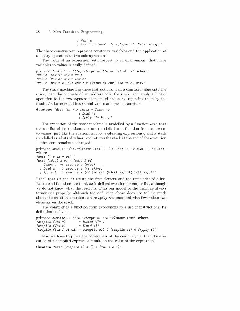
38 3. More Functional Programming
| Vex ’a| Bex "’v binop" "(’a,’v)expr" "(’a,’v)expr"
The three constructors represent constants, variables and the application ofa binary operation to two subexpressions.
The value of an expression with respect to an environment that mapsvariables to values is easily defined:
primrec "value" :: "(’a,’v)expr ⇒ (’a ⇒ ’v) ⇒ ’v" where"value (Cex v) env = v" |"value (Vex a) env = env a" |"value (Bex f e1 e2) env = f (value e1 env) (value e2 env)"
The stack machine has three instructions: load a constant value onto thestack, load the contents of an address onto the stack, and apply a binaryoperation to the two topmost elements of the stack, replacing them by theresult. As for expr, addresses and values are type parameters:
datatype (dead ’a, ’v) instr = Const ’v| Load ’a| Apply "’v binop"
The execution of the stack machine is modelled by a function exec thattakes a list of instructions, a store (modelled as a function from addressesto values, just like the environment for evaluating expressions), and a stack(modelled as a list) of values, and returns the stack at the end of the execution— the store remains unchanged:
primrec exec :: "(’a,’v)instr list ⇒ (’a⇒’v) ⇒ ’v list ⇒ ’v list"where"exec [] s vs = vs" |"exec (i#is) s vs = (case i of
Const v ⇒ exec is s (v#vs)| Load a ⇒ exec is s ((s a)#vs)| Apply f ⇒ exec is s ((f (hd vs) (hd(tl vs)))#(tl(tl vs))))"
Recall that hd and tl return the first element and the remainder of a list.Because all functions are total, hd is defined even for the empty list, althoughwe do not know what the result is. Thus our model of the machine alwaysterminates properly, although the definition above does not tell us muchabout the result in situations where Apply was executed with fewer than twoelements on the stack.
The compiler is a function from expressions to a list of instructions. Itsdefinition is obvious:
primrec compile :: "(’a,’v)expr ⇒ (’a,’v)instr list" where"compile (Cex v) = [Const v]" |"compile (Vex a) = [Load a]" |"compile (Bex f e1 e2) = (compile e2) @ (compile e1) @ [Apply f]"
Now we have to prove the correctness of the compiler, i.e. that the exe-cution of a compiled expression results in the value of the expression:
theorem "exec (compile e) s [] = [value e s]"
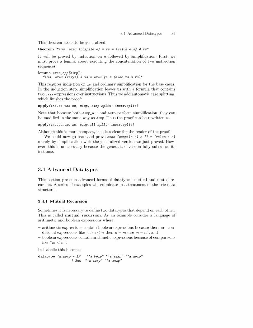
3.4 Advanced Datatypes 39
This theorem needs to be generalized:
theorem "∀ vs. exec (compile e) s vs = (value e s) # vs"
It will be proved by induction on e followed by simplification. First, wemust prove a lemma about executing the concatenation of two instructionsequences:
lemma exec_app[simp]:"∀ vs. exec (xs@ys) s vs = exec ys s (exec xs s vs)"
This requires induction on xs and ordinary simplification for the base cases.In the induction step, simplification leaves us with a formula that containstwo case -expressions over instructions. Thus we add automatic case splitting,which finishes the proof:
apply(induct_tac xs, simp, simp split: instr.split)
Note that because both simp_all and auto perform simplification, they canbe modified in the same way as simp. Thus the proof can be rewritten as
apply(induct_tac xs, simp_all split: instr.split)
Although this is more compact, it is less clear for the reader of the proof.We could now go back and prove exec (compile e) s [] = [value e s]
merely by simplification with the generalized version we just proved. How-ever, this is unnecessary because the generalized version fully subsumes itsinstance.
3.4 Advanced Datatypes
This section presents advanced forms of datatypes: mutual and nested re-cursion. A series of examples will culminate in a treatment of the trie datastructure.
3.4.1 Mutual Recursion
Sometimes it is necessary to define two datatypes that depend on each other.This is called mutual recursion. As an example consider a language ofarithmetic and boolean expressions where
– arithmetic expressions contain boolean expressions because there are con-ditional expressions like “if m < n then n −m else m − n”, and
– boolean expressions contain arithmetic expressions because of comparisonslike “m < n”.
In Isabelle this becomes
datatype ’a aexp = IF "’a bexp" "’a aexp" "’a aexp"| Sum "’a aexp" "’a aexp"
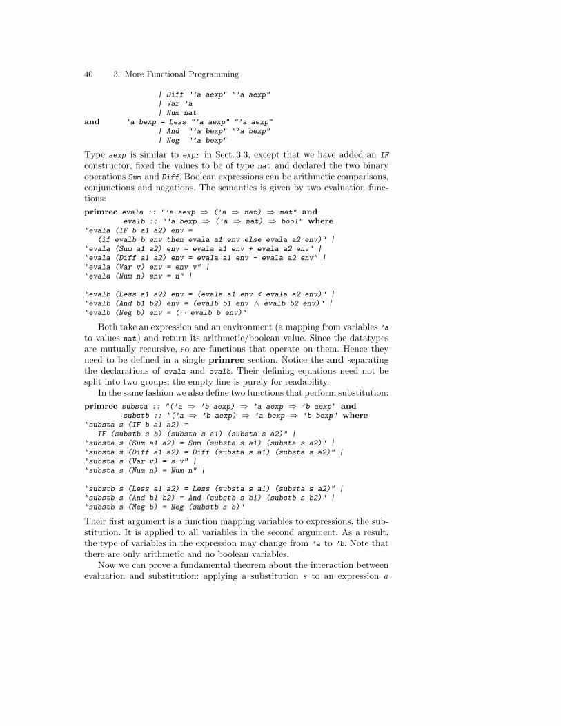
40 3. More Functional Programming
| Diff "’a aexp" "’a aexp"| Var ’a| Num nat
and ’a bexp = Less "’a aexp" "’a aexp"| And "’a bexp" "’a bexp"| Neg "’a bexp"
Type aexp is similar to expr in Sect. 3.3, except that we have added an IF
constructor, fixed the values to be of type nat and declared the two binaryoperations Sum and Diff. Boolean expressions can be arithmetic comparisons,conjunctions and negations. The semantics is given by two evaluation func-tions:
primrec evala :: "’a aexp ⇒ (’a ⇒ nat) ⇒ nat" andevalb :: "’a bexp ⇒ (’a ⇒ nat) ⇒ bool" where
"evala (IF b a1 a2) env =(if evalb b env then evala a1 env else evala a2 env)" |
"evala (Sum a1 a2) env = evala a1 env + evala a2 env" |"evala (Diff a1 a2) env = evala a1 env - evala a2 env" |"evala (Var v) env = env v" |"evala (Num n) env = n" |
"evalb (Less a1 a2) env = (evala a1 env < evala a2 env)" |"evalb (And b1 b2) env = (evalb b1 env ∧ evalb b2 env)" |"evalb (Neg b) env = (¬ evalb b env)"
Both take an expression and an environment (a mapping from variables ’ato values nat) and return its arithmetic/boolean value. Since the datatypesare mutually recursive, so are functions that operate on them. Hence theyneed to be defined in a single primrec section. Notice the and separatingthe declarations of evala and evalb. Their defining equations need not besplit into two groups; the empty line is purely for readability.
In the same fashion we also define two functions that perform substitution:
primrec substa :: "(’a ⇒ ’b aexp) ⇒ ’a aexp ⇒ ’b aexp" andsubstb :: "(’a ⇒ ’b aexp) ⇒ ’a bexp ⇒ ’b bexp" where
"substa s (IF b a1 a2) =IF (substb s b) (substa s a1) (substa s a2)" |
"substa s (Sum a1 a2) = Sum (substa s a1) (substa s a2)" |"substa s (Diff a1 a2) = Diff (substa s a1) (substa s a2)" |"substa s (Var v) = s v" |"substa s (Num n) = Num n" |
"substb s (Less a1 a2) = Less (substa s a1) (substa s a2)" |"substb s (And b1 b2) = And (substb s b1) (substb s b2)" |"substb s (Neg b) = Neg (substb s b)"
Their first argument is a function mapping variables to expressions, the sub-stitution. It is applied to all variables in the second argument. As a result,the type of variables in the expression may change from ’a to ’b. Note thatthere are only arithmetic and no boolean variables.
Now we can prove a fundamental theorem about the interaction betweenevaluation and substitution: applying a substitution s to an expression a
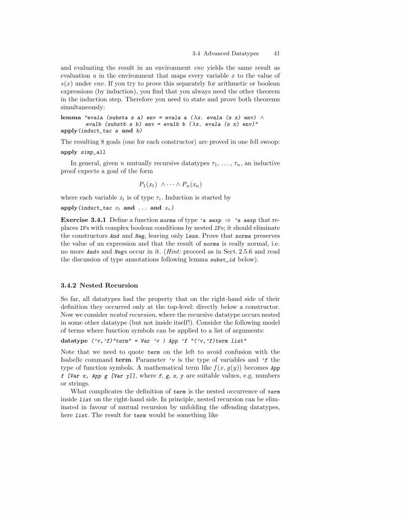
3.4 Advanced Datatypes 41
and evaluating the result in an environment env yields the same result asevaluation a in the environment that maps every variable x to the value ofs(x ) under env . If you try to prove this separately for arithmetic or booleanexpressions (by induction), you find that you always need the other theoremin the induction step. Therefore you need to state and prove both theoremssimultaneously:
lemma "evala (substa s a) env = evala a (λx. evala (s x) env) ∧evalb (substb s b) env = evalb b (λx. evala (s x) env)"
apply(induct_tac a and b)
The resulting 8 goals (one for each constructor) are proved in one fell swoop:
apply simp_all
In general, given n mutually recursive datatypes τ1, . . . , τn , an inductiveproof expects a goal of the form
P1(x1) ∧ · · · ∧ Pn(xn)
where each variable xi is of type τi . Induction is started by
apply(induct_tac x1 and ... and xn)
Exercise 3.4.1 Define a function norma of type ’a aexp ⇒ ’a aexp that re-places IFs with complex boolean conditions by nested IFs; it should eliminatethe constructors And and Neg, leaving only Less. Prove that norma preservesthe value of an expression and that the result of norma is really normal, i.e.no more Ands and Negs occur in it. (Hint: proceed as in Sect. 2.5.6 and readthe discussion of type annotations following lemma subst_id below).
3.4.2 Nested Recursion
So far, all datatypes had the property that on the right-hand side of theirdefinition they occurred only at the top-level: directly below a constructor.Now we consider nested recursion, where the recursive datatype occurs nestedin some other datatype (but not inside itself!). Consider the following modelof terms where function symbols can be applied to a list of arguments:
datatype (’v,’f)"term" = Var ’v | App ’f "(’v,’f)term list"
Note that we need to quote term on the left to avoid confusion with theIsabelle command term. Parameter ’v is the type of variables and ’f thetype of function symbols. A mathematical term like f (x , g(y)) becomes App
f [Var x, App g [Var y]], where f, g, x, y are suitable values, e.g. numbersor strings.
What complicates the definition of term is the nested occurrence of terminside list on the right-hand side. In principle, nested recursion can be elim-inated in favour of mutual recursion by unfolding the offending datatypes,here list. The result for term would be something like
42 3. More Functional Programming
datatype (’v,’f)"term" = Var ’v | App ’f "(’v,’f)term_list"and (’v,’f)term_list = Nil | Cons "(’v,’f)term" "(’v,’f)term_list"
Although we do not recommend this unfolding to the user, it shows how tosimulate nested recursion by mutual recursion. Now we return to the initialdefinition of term using nested recursion.
Let us define a substitution function on terms. Because terms involve termlists, we need to define two substitution functions simultaneously:
primrecsubst :: "(’v⇒(’v,’f)term) ⇒ (’v,’f)term ⇒ (’v,’f)term" andsubsts:: "(’v⇒(’v,’f)term) ⇒ (’v,’f)term list ⇒ (’v,’f)term list"where"subst s (Var x) = s x" |
subst_App:"subst s (App f ts) = App f (substs s ts)" |
"substs s [] = []" |"substs s (t # ts) = subst s t # substs s ts"
Individual equations in a primrec definition may be named as shown forsubst_App. The significance of this device will become apparent below.
Similarly, when proving a statement about terms inductively, we needto prove a related statement about term lists simultaneously. For example,the fact that the identity substitution does not change a term needs to bestrengthened and proved as follows:
lemma subst_id: "subst Var t = (t ::(’v,’f)term) ∧substs Var ts = (ts::(’v,’f)term list)"
apply(induct_tac t and ts rule: subst.induct substs.induct, simp_all)done
Note that Var is the identity substitution because by definition it leaves vari-ables unchanged: subst Var (Var x) = Var x. Note also that the type anno-tations are necessary because otherwise there is nothing in the goal to enforcethat both halves of the goal talk about the same type parameters (’v,’f).As a result, induction would fail because the two halves of the goal would beunrelated.
Exercise 3.4.2 The fact that substitution distributes over composition canbe expressed roughly as follows:
subst (f ◦ g) t = subst f (subst g t)
Correct this statement (you will find that it does not type-check), strengthenit, and prove it. (Note: ◦ is function composition; its definition is found intheorem o_def).
Exercise 3.4.3 Define a function trev of type (’v, ’f) Nested.term ⇒(’v, ’f) Nested.term that recursively reverses the order of arguments of allfunction symbols in a term. Prove that trev (trev t) = t.
3.4 Advanced Datatypes 43
The experienced functional programmer may feel that our definition ofsubst is too complicated in that substs is unnecessary. The App -case can bedefined directly as
subst s (App f ts) = App f (map (subst s) ts)
where map is the standard list function such that map f [x1,...,xn] = [f
x1,...,f xn]. This is true, but Isabelle insists on the conjunctive format.Fortunately, we can easily prove that the suggested equation holds:
lemma [simp]: "subst s (App f ts) = App f (map (subst s) ts)"apply(induct_tac ts, simp_all)done
What is more, we can now disable the old defining equation as a simplificationrule:
declare subst_App [simp del]
The advantage is that now we have replaced substs by map, we can profit fromthe large number of pre-proved lemmas about map. Unfortunately, inductiveproofs about type term are still awkward because they expect a conjunc-tion. One could derive a new induction principle as well (see Sect. 9.2.3), butsimpler is to stop using primrec and to define functions with fun instead.Simple uses of fun are described in Sect. 3.5 below. Advanced applications,including functions over nested datatypes like term, are discussed in a sepa-rate tutorial [18].
Of course, you may also combine mutual and nested recursion of data-types. For example, constructor Sum in Sect. 3.4.1 could take a list of expres-sions as its argument: Sum "’a aexp list".
3.4.3 The Limits of Nested Recursion
How far can we push nested recursion? By the unfolding argument above,we can reduce nested to mutual recursion provided the nested recursion onlyinvolves previously defined datatypes. This does not include functions:
datatype t = C "t ⇒ bool"
This declaration is a real can of worms. In HOL it must be ruled out becauseit requires a type t such that t and its power set t ⇒ bool have the samecardinality — an impossibility. For the same reason it is not possible to allowrecursion involving the type t set, which is isomorphic to t ⇒ bool.
Fortunately, a limited form of recursion involving function spaces is per-mitted: the recursive type may occur on the right of a function arrow, butnever on the left. Hence the above can of worms is ruled out but the followingexample of a potentially infinitely branching tree is accepted:
datatype (dead ’a,’i) bigtree = Tip | Br ’a "’i ⇒ (’a,’i)bigtree"
44 3. More Functional Programming
Parameter ’a is the type of values stored in the Branches of the tree, whereas’i is the index type over which the tree branches. If ’i is instantiated to bool,the result is a binary tree; if it is instantiated to nat, we have an infinitelybranching tree because each node has as many subtrees as there are naturalnumbers. How can we possibly write down such a tree? Using functionalnotation! For example, the term
Br 0 (λi. Br i (λn. Tip))
of type (nat, nat) bigtree is the tree whose root is labeled with 0 and whoseith subtree is labeled with i and has merely Tips as further subtrees.
Function map_bt applies a function to all labels in a bigtree :
primrec map_bt :: "(’a ⇒ ’b) ⇒ (’a,’i)bigtree ⇒ (’b,’i)bigtree"where"map_bt f Tip = Tip" |"map_bt f (Br a F) = Br (f a) (λi. map_bt f (F i))"
This is a valid primrec definition because the recursive calls of map_bt in-volve only subtrees of F, which is itself a subterm of the left-hand side. Thustermination is assured. The seasoned functional programmer might try ex-pressing λi. map_bt f (F i) as map_bt f ◦ F, which Isabelle however willreject. Applying map_bt to only one of its arguments makes the terminationproof less obvious.
The following lemma has a simple proof by induction:
lemma "map_bt (g o f) T = map_bt g (map_bt f T)"apply(induct_tac T, simp_all)done
Because of the function type, the proof state after induction looks unusual.Notice the quantified induction hypothesis:
1. map_bt (g ◦ f) Tip = map_bt g (map_bt f Tip)2.
∧x1 F.(∧x2a. x2a ∈ range F =⇒
map_bt (g ◦ f) x2a = map_bt g (map_bt f x2a)) =⇒map_bt (g ◦ f) (Br x1 F) = map_bt g (map_bt f (Br x1 F))
If you need nested recursion on the left of a function arrow, there arealternatives to pure HOL. In the Logic for Computable Functions (LCF),types like
datatype lam = C "lam → lam"
do indeed make sense [28]. Note the different arrow,→ instead of ⇒, express-ing the type of continuous functions. There is even a version of LCF on topof HOL, called HOLCF [21].
3.4.4 Case Study: Tries
Tries are a classic search tree data structure [17] for fast indexing with strings.Figure 3.1 gives a graphical example of a trie containing the words “all”, “an”,
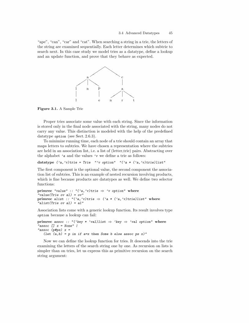
3.4 Advanced Datatypes 45
“ape”, “can”, “car” and “cat”. When searching a string in a trie, the letters ofthe string are examined sequentially. Each letter determines which subtrie tosearch next. In this case study we model tries as a datatype, define a lookupand an update function, and prove that they behave as expected.
l e n r t
���
QQQ
l n p a
���
QQQ
a c
��
��
QQQQ
Figure 3.1. A Sample Trie
Proper tries associate some value with each string. Since the informationis stored only in the final node associated with the string, many nodes do notcarry any value. This distinction is modeled with the help of the predefineddatatype option (see Sect. 2.6.3).
To minimize running time, each node of a trie should contain an array thatmaps letters to subtries. We have chosen a representation where the subtriesare held in an association list, i.e. a list of (letter,trie) pairs. Abstracting overthe alphabet ’a and the values ’v we define a trie as follows:
datatype (’a,’v)trie = Trie "’v option" "(’a * (’a,’v)trie)list"
The first component is the optional value, the second component the associa-tion list of subtries. This is an example of nested recursion involving products,which is fine because products are datatypes as well. We define two selectorfunctions:
primrec "value" :: "(’a,’v)trie ⇒ ’v option" where"value(Trie ov al) = ov"primrec alist :: "(’a,’v)trie ⇒ (’a * (’a,’v)trie)list" where"alist(Trie ov al) = al"
Association lists come with a generic lookup function. Its result involves typeoption because a lookup can fail:
primrec assoc :: "(’key * ’val)list ⇒ ’key ⇒ ’val option" where"assoc [] x = None" |"assoc (p#ps) x =
(let (a,b) = p in if a=x then Some b else assoc ps x)"
Now we can define the lookup function for tries. It descends into the trieexamining the letters of the search string one by one. As recursion on lists issimpler than on tries, let us express this as primitive recursion on the searchstring argument:
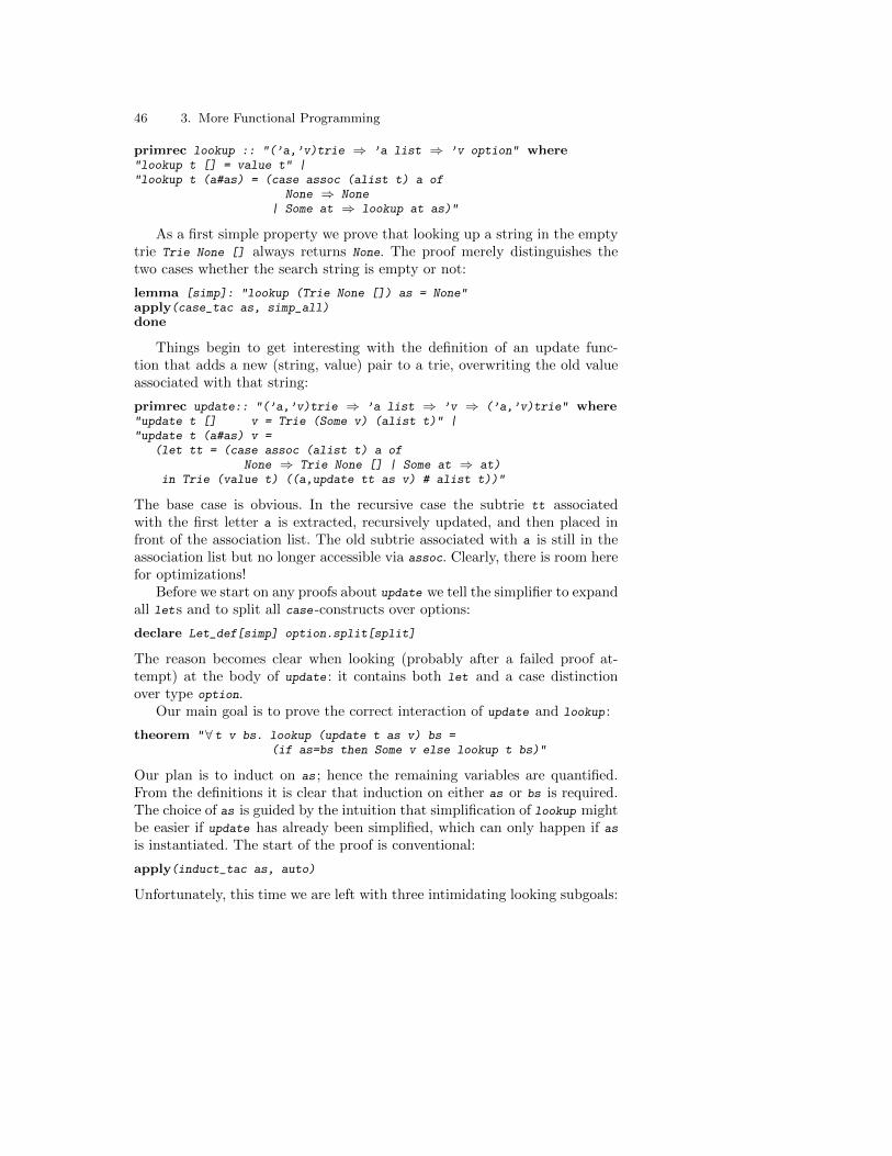
46 3. More Functional Programming
primrec lookup :: "(’a,’v)trie ⇒ ’a list ⇒ ’v option" where"lookup t [] = value t" |"lookup t (a#as) = (case assoc (alist t) a of
None ⇒ None| Some at ⇒ lookup at as)"
As a first simple property we prove that looking up a string in the emptytrie Trie None [] always returns None. The proof merely distinguishes thetwo cases whether the search string is empty or not:
lemma [simp]: "lookup (Trie None []) as = None"apply(case_tac as, simp_all)done
Things begin to get interesting with the definition of an update func-tion that adds a new (string, value) pair to a trie, overwriting the old valueassociated with that string:
primrec update:: "(’a,’v)trie ⇒ ’a list ⇒ ’v ⇒ (’a,’v)trie" where"update t [] v = Trie (Some v) (alist t)" |"update t (a#as) v =
(let tt = (case assoc (alist t) a ofNone ⇒ Trie None [] | Some at ⇒ at)
in Trie (value t) ((a,update tt as v) # alist t))"
The base case is obvious. In the recursive case the subtrie tt associatedwith the first letter a is extracted, recursively updated, and then placed infront of the association list. The old subtrie associated with a is still in theassociation list but no longer accessible via assoc. Clearly, there is room herefor optimizations!
Before we start on any proofs about update we tell the simplifier to expandall lets and to split all case -constructs over options:
declare Let_def[simp] option.split[split]
The reason becomes clear when looking (probably after a failed proof at-tempt) at the body of update : it contains both let and a case distinctionover type option.
Our main goal is to prove the correct interaction of update and lookup :
theorem "∀ t v bs. lookup (update t as v) bs =(if as=bs then Some v else lookup t bs)"
Our plan is to induct on as ; hence the remaining variables are quantified.From the definitions it is clear that induction on either as or bs is required.The choice of as is guided by the intuition that simplification of lookup mightbe easier if update has already been simplified, which can only happen if asis instantiated. The start of the proof is conventional:
apply(induct_tac as, auto)
Unfortunately, this time we are left with three intimidating looking subgoals:
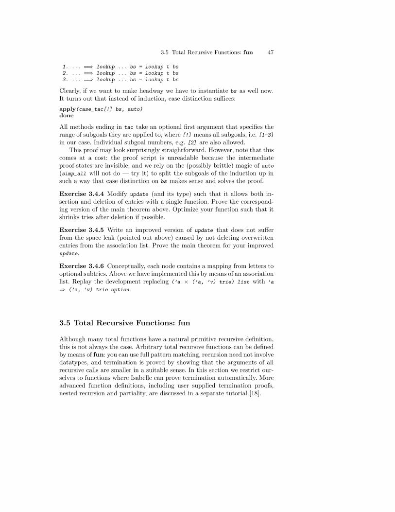
3.5 Total Recursive Functions: fun 47
1. ... =⇒ lookup ... bs = lookup t bs2. ... =⇒ lookup ... bs = lookup t bs3. ... =⇒ lookup ... bs = lookup t bs
Clearly, if we want to make headway we have to instantiate bs as well now.It turns out that instead of induction, case distinction suffices:
apply(case_tac[!] bs, auto)done
All methods ending in tac take an optional first argument that specifies therange of subgoals they are applied to, where [!] means all subgoals, i.e. [1-3]in our case. Individual subgoal numbers, e.g. [2] are also allowed.
This proof may look surprisingly straightforward. However, note that thiscomes at a cost: the proof script is unreadable because the intermediateproof states are invisible, and we rely on the (possibly brittle) magic of auto(simp_all will not do — try it) to split the subgoals of the induction up insuch a way that case distinction on bs makes sense and solves the proof.
Exercise 3.4.4 Modify update (and its type) such that it allows both in-sertion and deletion of entries with a single function. Prove the correspond-ing version of the main theorem above. Optimize your function such that itshrinks tries after deletion if possible.
Exercise 3.4.5 Write an improved version of update that does not sufferfrom the space leak (pointed out above) caused by not deleting overwrittenentries from the association list. Prove the main theorem for your improvedupdate.
Exercise 3.4.6 Conceptually, each node contains a mapping from letters tooptional subtries. Above we have implemented this by means of an associationlist. Replay the development replacing (’a × (’a, ’v) trie) list with ’a
⇒ (’a, ’v) trie option.
3.5 Total Recursive Functions: fun
Although many total functions have a natural primitive recursive definition,this is not always the case. Arbitrary total recursive functions can be definedby means of fun: you can use full pattern matching, recursion need not involvedatatypes, and termination is proved by showing that the arguments of allrecursive calls are smaller in a suitable sense. In this section we restrict our-selves to functions where Isabelle can prove termination automatically. Moreadvanced function definitions, including user supplied termination proofs,nested recursion and partiality, are discussed in a separate tutorial [18].
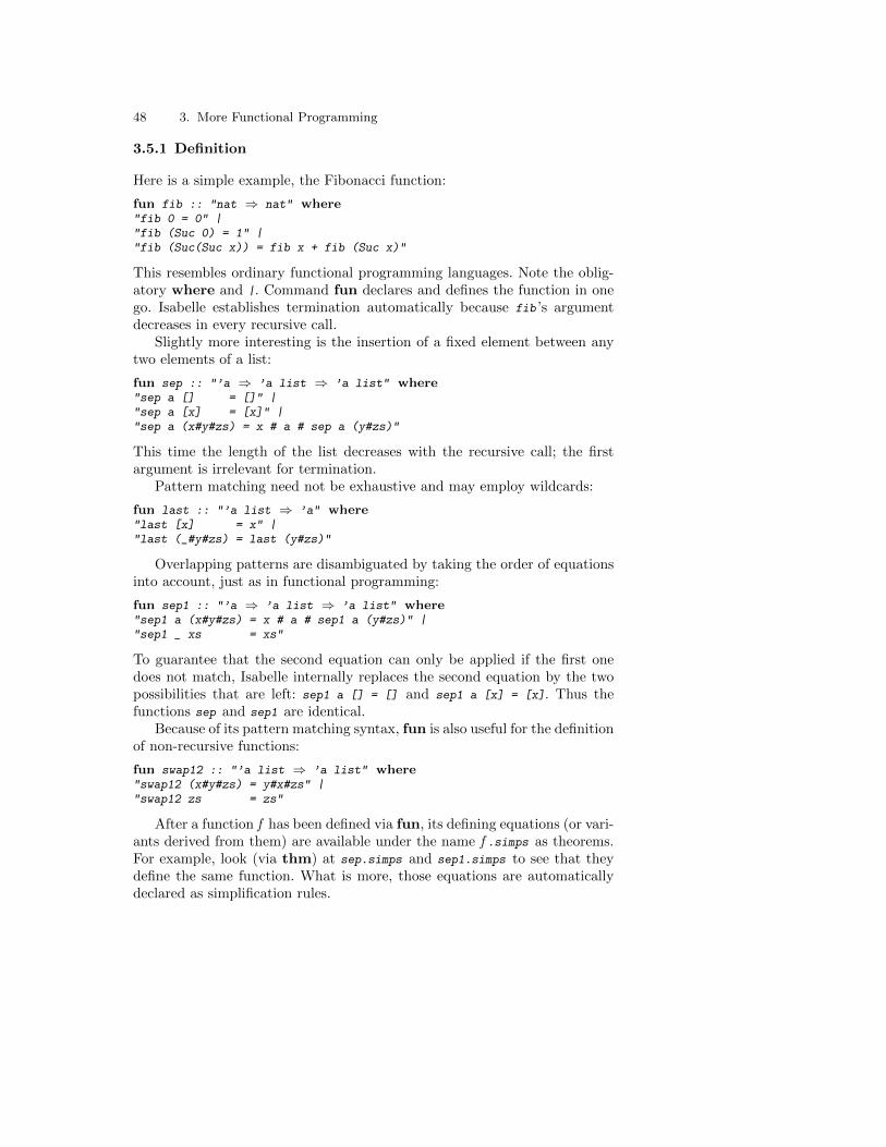
48 3. More Functional Programming
3.5.1 Definition
Here is a simple example, the Fibonacci function:
fun fib :: "nat ⇒ nat" where"fib 0 = 0" |"fib (Suc 0) = 1" |"fib (Suc(Suc x)) = fib x + fib (Suc x)"
This resembles ordinary functional programming languages. Note the oblig-atory where and |. Command fun declares and defines the function in onego. Isabelle establishes termination automatically because fib ’s argumentdecreases in every recursive call.
Slightly more interesting is the insertion of a fixed element between anytwo elements of a list:
fun sep :: "’a ⇒ ’a list ⇒ ’a list" where"sep a [] = []" |"sep a [x] = [x]" |"sep a (x#y#zs) = x # a # sep a (y#zs)"
This time the length of the list decreases with the recursive call; the firstargument is irrelevant for termination.
Pattern matching need not be exhaustive and may employ wildcards:
fun last :: "’a list ⇒ ’a" where"last [x] = x" |"last (_#y#zs) = last (y#zs)"
Overlapping patterns are disambiguated by taking the order of equationsinto account, just as in functional programming:
fun sep1 :: "’a ⇒ ’a list ⇒ ’a list" where"sep1 a (x#y#zs) = x # a # sep1 a (y#zs)" |"sep1 _ xs = xs"
To guarantee that the second equation can only be applied if the first onedoes not match, Isabelle internally replaces the second equation by the twopossibilities that are left: sep1 a [] = [] and sep1 a [x] = [x]. Thus thefunctions sep and sep1 are identical.
Because of its pattern matching syntax, fun is also useful for the definitionof non-recursive functions:
fun swap12 :: "’a list ⇒ ’a list" where"swap12 (x#y#zs) = y#x#zs" |"swap12 zs = zs"
After a function f has been defined via fun, its defining equations (or vari-ants derived from them) are available under the name f .simps as theorems.For example, look (via thm) at sep.simps and sep1.simps to see that theydefine the same function. What is more, those equations are automaticallydeclared as simplification rules.
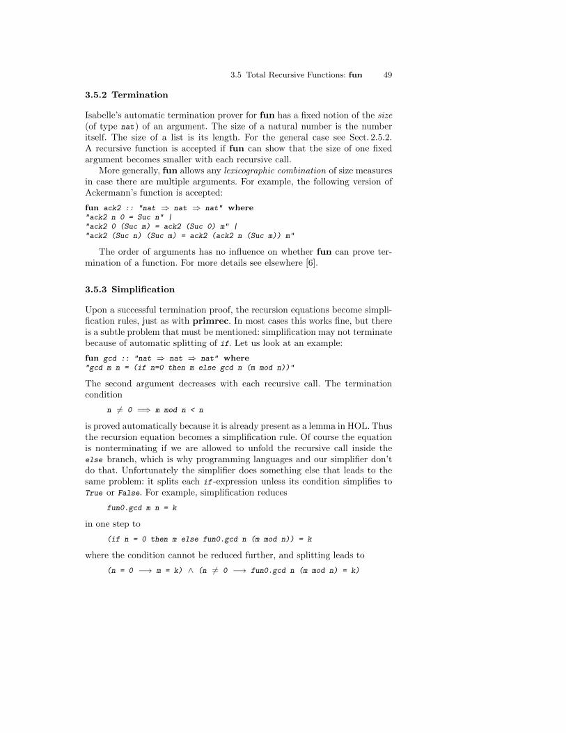
3.5 Total Recursive Functions: fun 49
3.5.2 Termination
Isabelle’s automatic termination prover for fun has a fixed notion of the size(of type nat) of an argument. The size of a natural number is the numberitself. The size of a list is its length. For the general case see Sect. 2.5.2.A recursive function is accepted if fun can show that the size of one fixedargument becomes smaller with each recursive call.
More generally, fun allows any lexicographic combination of size measuresin case there are multiple arguments. For example, the following version ofAckermann’s function is accepted:
fun ack2 :: "nat ⇒ nat ⇒ nat" where"ack2 n 0 = Suc n" |"ack2 0 (Suc m) = ack2 (Suc 0) m" |"ack2 (Suc n) (Suc m) = ack2 (ack2 n (Suc m)) m"
The order of arguments has no influence on whether fun can prove ter-mination of a function. For more details see elsewhere [6].
3.5.3 Simplification
Upon a successful termination proof, the recursion equations become simpli-fication rules, just as with primrec. In most cases this works fine, but thereis a subtle problem that must be mentioned: simplification may not terminatebecause of automatic splitting of if. Let us look at an example:
fun gcd :: "nat ⇒ nat ⇒ nat" where"gcd m n = (if n=0 then m else gcd n (m mod n))"
The second argument decreases with each recursive call. The terminationcondition
n 6= 0 =⇒ m mod n < n
is proved automatically because it is already present as a lemma in HOL. Thusthe recursion equation becomes a simplification rule. Of course the equationis nonterminating if we are allowed to unfold the recursive call inside theelse branch, which is why programming languages and our simplifier don’tdo that. Unfortunately the simplifier does something else that leads to thesame problem: it splits each if -expression unless its condition simplifies toTrue or False. For example, simplification reduces
fun0.gcd m n = k
in one step to
(if n = 0 then m else fun0.gcd n (m mod n)) = k
where the condition cannot be reduced further, and splitting leads to
(n = 0 −→ m = k) ∧ (n 6= 0 −→ fun0.gcd n (m mod n) = k)
50 3. More Functional Programming
Since the recursive call fun0.gcd n (m mod n) is no longer protected by an if,it is unfolded again, which leads to an infinite chain of simplification steps.Fortunately, this problem can be avoided in many different ways.
The most radical solution is to disable the offending theorem if_split,as shown in Sect. 3.1.9. However, we do not recommend this approach: youwill often have to invoke the rule explicitly when if is involved.
If possible, the definition should be given by pattern matching on the leftrather than if on the right. In the case of fun0.gcd the following alternativedefinition suggests itself:
fun gcd1 :: "nat ⇒ nat ⇒ nat" where"gcd1 m 0 = m" |"gcd1 m n = gcd1 n (m mod n)"
The order of equations is important: it hides the side condition n 6= 0. Un-fortunately, not all conditionals can be expressed by pattern matching.
A simple alternative is to replace if by case, which is also available forbool and is not split automatically:
fun gcd2 :: "nat ⇒ nat ⇒ nat" where"gcd2 m n = (case n=0 of True ⇒ m | False ⇒ gcd2 n (m mod n))"
This is probably the neatest solution next to pattern matching, and it isalways available.
A final alternative is to replace the offending simplification rules by de-rived conditional ones. For fun0.gcd it means we have to prove these lemmas:
lemma [simp]: "gcd m 0 = m"apply(simp)done
lemma [simp]: "n 6= 0 =⇒ gcd m n = gcd n (m mod n)"apply(simp)done
Simplification terminates for these proofs because the condition of the if
simplifies to True or False. Now we can disable the original simplificationrule:
declare gcd.simps [simp del]
3.5.4 Induction
Having defined a function we might like to prove something about it. Since thefunction is recursive, the natural proof principle is again induction. But thistime the structural form of induction that comes with datatypes is unlikelyto work well — otherwise we could have defined the function by primrec.Therefore fun automatically proves a suitable induction rule f .induct thatfollows the recursion pattern of the particular function f . We call this re-cursion induction. Roughly speaking, it requires you to prove for each fun
3.5 Total Recursive Functions: fun 51
equation that the property you are trying to establish holds for the left-handside provided it holds for all recursive calls on the right-hand side. Here is asimple example involving the predefined map functional on lists:
lemma "map f (sep x xs) = sep (f x) (map f xs)"
Note that map f xs is the result of applying f to all elements of xs. We provethis lemma by recursion induction over sep :
apply(induct_tac x xs rule: sep.induct)
The resulting proof state has three subgoals corresponding to the threeclauses for sep :
1.∧a. map f (sep a []) = sep (f a) (map f [])
2.∧a x. map f (sep a [x]) = sep (f a) (map f [x])
3.∧a x y zs.map f (sep a (y # zs)) = sep (f a) (map f (y # zs)) =⇒map f (sep a (x # y # zs)) = sep (f a) (map f (x # y # zs))
The rest is pure simplification:
apply simp_alldone
The proof goes smoothly because the induction rule follows the recursion ofsep. Try proving the above lemma by structural induction, and you find thatyou need an additional case distinction.
In general, the format of invoking recursion induction is
apply(induct_tac x1 . . . xn rule: f .induct)
where x1 . . . xn is a list of free variables in the subgoal and f the name of afunction that takes n arguments. Usually the subgoal will contain the termfx1 . . . xn but this need not be the case. The induction rules do not mentionf at all. Here is sep.induct :
[[∧a. P a [];∧a x. P a [x];∧a x y zs. P a (y # zs) =⇒ P a (x # y # zs) ]]
=⇒ P u v
It merely says that in order to prove a property P of u and v you need toprove it for the three cases where v is the empty list, the singleton list, andthe list with at least two elements. The final case has an induction hypothesis:you may assume that P holds for the tail of that list.

4. Presenting Theories
By now the reader should have become sufficiently acquainted with elemen-tary theory development in Isabelle/HOL. The following interlude describeshow to present theories in a typographically pleasing manner. Isabelle pro-vides a rich infrastructure for concrete syntax of the underlying λ-calculuslanguage (see Sect. 4.1), as well as document preparation of theory texts basedon existing PDF-LATEX technology (see Sect. 4.2).
As pointed out by Leibniz more than 300 years ago, notions are in princi-ple more important than notations, but suggestive textual representation ofideas is vital to reduce the mental effort to comprehend and apply them.
4.1 Concrete Syntax
The core concept of Isabelle’s framework for concrete syntax is that of mixfixannotations. Associated with any kind of constant declaration, mixfixesaffect both the grammar productions for the parser and output templates forthe pretty printer.
In full generality, parser and pretty printer configuration is a subtle af-fair [38]. Your syntax specifications need to interact properly with the existingsetup of Isabelle/Pure and Isabelle/HOL. To avoid creating ambiguities withexisting elements, it is particularly important to give new syntactic constructsthe right precedence.
Below we introduce a few simple syntax declaration forms that alreadycover many common situations fairly well.
4.1.1 Infix Annotations
Syntax annotations may be included wherever constants are declared, such asdefinition and primrec — and also datatype, which declares constructoroperations. Type-constructors may be annotated as well, although this is lessfrequently encountered in practice (the infix type × comes to mind).
Infix declarations provide a useful special case of mixfixes. The followingexample of the exclusive-or operation on boolean values illustrates typicalinfix declarations.
54 4. Presenting Theories
definition xor :: "bool ⇒ bool ⇒ bool" ( infixl "[+]" 60)where "A [+] B ≡ (A ∧ ¬ B) ∨ (¬ A ∧ B)"
Now xor A B and A [+] B refer to the same expression internally. Any cur-ried function with at least two arguments may be given infix syntax. Forpartial applications with fewer than two operands, the operator is enclosedin parentheses. For instance, xor without arguments is represented as ([+]) ;together with ordinary function application, this turns xor A into ([+]) A.
The keyword infixl seen above specifies an infix operator that is nestedto the left : in iterated applications the more complex expression appears onthe left-hand side, and A [+] B [+] C stands for (A [+] B) [+] C. Similarly,infixr means nesting to the right, reading A [+] B [+] C as A [+] (B [+] C).A non-oriented declaration via infix would render A [+] B [+] C illegal, butdemand explicit parentheses to indicate the intended grouping.
The string [+] in our annotation refers to the concrete syntax to rep-resent the operator (a literal token), while the number 60 determines theprecedence of the construct: the syntactic priorities of the arguments andresult. Isabelle/HOL already uses up many popular combinations of ASCIIsymbols for its own use, including both + and ++. Longer character combina-tions are more likely to be still available for user extensions, such as our [+].
Operator precedences have a range of 0–1000. Very low or high prioritiesare reserved for the meta-logic. HOL syntax mainly uses the range of 10–100:the equality infix = is centered at 50; logical connectives (like ∨ and ∧) arebelow 50; algebraic ones (like + and *) are above 50. User syntax shouldstrive to coexist with common HOL forms, or use the mostly unused range100–900.
4.1.2 Mathematical Symbols
Concrete syntax based on ASCII characters has inherent limitations. Math-ematical notation demands a larger repertoire of glyphs. Several standardsof extended character sets have been proposed over decades, but none hasbecome universally available so far. Isabelle has its own notion of symbolsas the smallest entities of source text, without referring to internal encodings.There are three kinds of such “generalized characters”:
1. 7-bit ASCII characters2. named symbols: \<ident>3. named control symbols: \<^ident>
Here ident is any sequence of letters. This results in an infinite store ofsymbols, whose interpretation is left to further front-end tools. For example,the Isabelle document processor (see Sect. 4.2) display the \<forall> symbolas ∀ .
A list of standard Isabelle symbols is given in [38]. You may introduceyour own interpretation of further symbols by configuring the appropriate
4.1 Concrete Syntax 55
front-end tool accordingly, e.g. by defining certain LATEX macros (see alsoSect. 4.2.4). There are also a few predefined control symbols, such as \<^sub>and \<^sup> for sub- and superscript of the subsequent printable symbol,respectively. For example, A\<^sup>\<star>, is output as A?.
A number of symbols are considered letters by the Isabelle lexer and canbe used as part of identifiers. These are the greek letters α (\<alpha>), β(\<beta>), etc. (excluding λ), special letters like A (\<A>) and A (\<AA>).Moreover the control symbol \<^sub> may be used to subscript a single letteror digit in the trailing part of an identifier. This means that the input
\<forall>\<alpha>\<^sub>1. \<alpha>\<^sub>1 = \<Pi>\<^sub>\<A>
is recognized as the term ∀α1. α1 = ΠA by Isabelle.Replacing our previous definition of xor by the following specifies an Isa-
belle symbol for the new operator:
definition xor :: "bool ⇒ bool ⇒ bool" ( infixl "⊕" 60)where "A ⊕ B ≡ (A ∧ ¬ B) ∨ (¬ A ∧ B)"
It is possible to provide alternative syntax forms through the print modeconcept [38]. By convention, the mode of “xsymbols” is enabled wheneverProof General’s X-Symbol mode or LATEX output is active. Now consider thefollowing hybrid declaration of xor :
definition xor :: "bool ⇒ bool ⇒ bool" ( infixl "[+]" 60)where "A [+] B ≡ (A ∧ ¬ B) ∨ (¬ A ∧ B)"
notation (xsymbols) xor ( infixl "⊕" 60)
The notation command associates a mixfix annotation with a known con-stant. The print mode specification, here (xsymbols), is optional.
We may now write A [+] B or A ⊕ B in input, while output uses the nicersyntax of xsymbols whenever that print mode is active. Such an arrange-ment is particularly useful for interactive development, where users may typeASCII text and see mathematical symbols displayed during proofs.
4.1.3 Prefix Annotations
Prefix syntax annotations are another form of mixfixes [38], without anytemplate arguments or priorities — just some literal syntax. The followingexample associates common symbols with the constructors of a datatype.
datatype currency =Euro nat ("e")
| Pounds nat ("£")| Yen nat ("U")| Dollar nat ("$")
Here the mixfix annotations on the rightmost column happen to consist of asingle Isabelle symbol each: \<euro>, \<pounds>, \<yen>, and $. Recall that
56 4. Presenting Theories
a constructor like Euro actually is a function nat ⇒ currency. The expressionEuro 10 will be printed as e 10 ; only the head of the application is subject toour concrete syntax. This rather simple form already achieves conformancewith notational standards of the European Commission.
Prefix syntax works the same way for other commands that introduce newconstants, e.g. primrec.
4.1.4 Abbreviations
Mixfix syntax annotations merely decorate particular constant applicationforms with concrete syntax, for instance replacing xor A B by A ⊕ B. Occa-sionally, the relationship between some piece of notation and its internal formis more complicated. Here we need abbreviations.
Command abbreviation introduces an uninterpreted notational constantas an abbreviation for a complex term. Abbreviations are unfolded uponparsing and re-introduced upon printing. This provides a simple mechanismfor syntactic macros.
A typical use of abbreviations is to introduce relational notation for mem-bership in a set of pairs, replacing (x, y) ∈ sim by x ≈ y. We assume thata constant sim of type (’a × ’a) set has been introduced at this point.
abbreviation sim2 :: "’a ⇒ ’a ⇒ bool" ( infix "≈" 50)where "x ≈ y ≡ (x, y) ∈ sim"
The given meta-equality is used as a rewrite rule after parsing (replacingx ≈ y by (x,y) ∈ sim) and before printing (turning (x,y) ∈ sim back intox ≈ y). The name of the dummy constant sim2 does not matter, as long asit is unique.
Another common application of abbreviations is to provide variant ver-sions of fundamental relational expressions, such as 6= for negated equalities.The following declaration stems from Isabelle/HOL itself:
abbreviation not_equal :: "’a ⇒ ’a ⇒ bool" ( infixl "~=" 50)where "x ~= y ≡ ¬ (x = y)"
notation (xsymbols) not_equal ( infix " 6=" 50)
The notation 6= is introduced separately to restrict it to the xsymbols mode.Abbreviations are appropriate when the defined concept is a simple vari-
ation on an existing one. But because of the automatic folding and unfoldingof abbreviations, they do not scale up well to large hierarchies of concepts.Abbreviations do not replace definitions.
Abbreviations are a simplified form of the general concept of syntax trans-lations; even heavier transformations may be written in ML [38].
4.2 Document Preparation 57
4.2 Document Preparation
Isabelle/Isar is centered around the concept of formal proof documents.The outcome of a formal development effort is meant to be a human-readablerecord, presented as browsable PDF file or printed on paper. The overalldocument structure follows traditional mathematical articles, with sections,intermediate explanations, definitions, theorems and proofs.
The Isabelle document preparation system essentially acts as a front-end to LATEX. After checking specifications and proofs formally, the theorysources are turned into typesetting instructions in a schematic manner. Thislets you write authentic reports on theory developments with little effort:many technical consistency checks are handled by the system.
Here is an example to illustrate the idea of Isabelle document preparation.
The following datatype definition of ’a bintree models binarytrees with nodes being decorated by elements of type ’a.
datatype ’a bintree =Leaf | Branch ’a "’a bintree" "’a bintree"
The datatype induction rule generated here is of the form
[[P Leaf;∧x1 x2 x3. [[P x2; P x3 ]] =⇒ P (Branch x1 x2 x3) ]] =⇒ P
bintree
The above document output has been produced as follows:
text {*The following datatype definition of @{text "’a bintree"}models binary trees with nodes being decorated by elementsof type @{typ ’a}.
*}
datatype ’a bintree =Leaf | Branch ’a "’a bintree" "’a bintree"
text {*\noindent The datatype induction rule generated here isof the form @{thm [display] bintree.induct [no_vars]}
*}
Here we have augmented the theory by formal comments (using text blocks),the informal parts may again refer to formal entities by means of “antiquota-tions” (such as @{text "’a bintree"} or @{typ ’a}), see also Sect. 4.2.3.
58 4. Presenting Theories
4.2.1 Isabelle Sessions
In contrast to the highly interactive mode of Isabelle/Isar theory develop-ment, the document preparation stage essentially works in batch-mode. AnIsabelle session consists of a collection of source files that may contribute toan output document. Each session is derived from a single parent, usually anobject-logic image like HOL. This results in an overall tree structure, whichis reflected by the output location in the file system (the root directory isdetermined by the Isabelle settings variable ISABELLE_BROWSER_INFO).
The easiest way to manage Isabelle sessions is via isabelle mkroot (togenerate an initial session source setup) and isabelle build (to run sessionsas specified in the corresponding ROOT file). These Isabelle tools are describedin further detail in the Isabelle System Manual [37].
For example, a new session MySession (with document preparation) maybe produced as follows:
isabelle mkroot MySession
isabelle build -D MySession
The isabelle build job also informs about the file-system location ofthe ultimate results. The above dry run should be able to produce somedocument.pdf (with dummy title, empty table of contents etc.). Any failureat this stage usually indicates technical problems of the LATEX installation.
The detailed arrangement of the session sources is as follows.
– Directory MySession holds the required theory files T1.thy, . . . , Tn.thy.– File MySession/ROOT specifies the session options and content, with decla-
rations for all wanted theories; it is sufficient to specify the terminal nodesof the theory dependency graph.
– Directory MySession/document contains everything required for the LATEXstage; only root.tex needs to be provided initially.The latter file holds appropriate LATEX code to commence a document(\documentclass etc.), and to include the generated files Ti.tex for eachtheory. Isabelle will generate a file session.tex holding LATEX commandsto include all generated theory output files in topologically sorted order, so\input{session} in the body of root.tex does the job in most situations.
One may now start to populate the directory MySession and its ROOT fileaccordingly. The file MySession/document/root.tex should also be adaptedat some point; the default version is mostly self-explanatory. Note that\isabellestyle enables fine-tuning of the general appearance of charactersand mathematical symbols (see also Sect. 4.2.4).
Especially observe the included LATEX packages isabelle (mandatory),isabellesym (required for mathematical symbols), and the final pdfsetup(provides sane defaults for hyperref, including URL markup). All three are
4.2 Document Preparation 59
distributed with Isabelle. Further packages may be required in particularapplications, say for unusual mathematical symbols.
Any additional files for the LATEX stage go into the MySession/document
directory as well. In particular, adding a file named root.bib causes an au-tomatic run of bibtex to process a bibliographic database; see also isabelle
document [37].
Any failure of the document preparation phase in an Isabelle batch ses-sion leaves the generated sources in their target location, identified by theaccompanying error message. This lets you trace LATEX problems with thegenerated files at hand.
4.2.2 Structure Markup
The large-scale structure of Isabelle documents follows existing LATEX conven-tions, with chapters, sections, subsubsections etc. The Isar language includesseparate markup commands, which do not affect the formal meaning of atheory (or proof), but result in corresponding LATEX elements.
From the Isabelle perspective, each markup command takes a single textargument (delimited by " . . . " or {* . . . *}). After stripping any surroundingwhite space, the argument is passed to a LATEX macro \isamarkupXYZ forcommand XYZ. These macros are defined in isabelle.sty according tothe meaning given in the rightmost column above.
The following source fragment illustrates structure markup of a theory.Note that LATEX labels may be included inside of section headings as well.
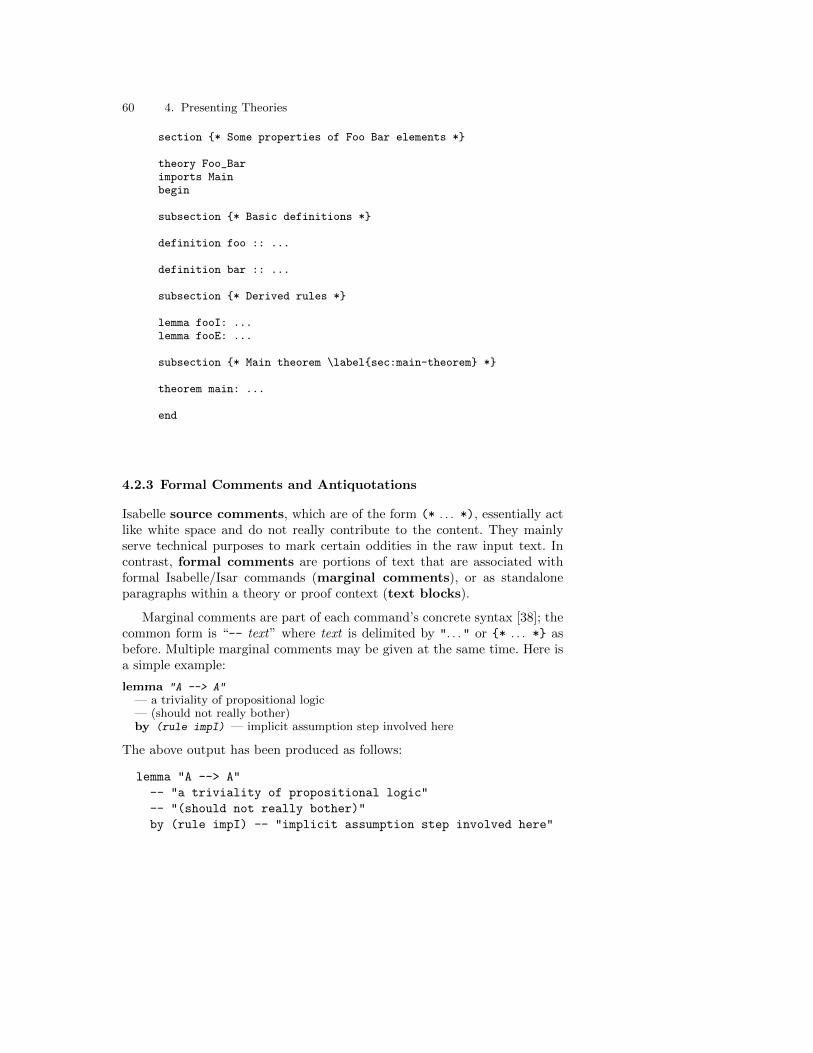
60 4. Presenting Theories
section {* Some properties of Foo Bar elements *}
theory Foo_Barimports Mainbegin
subsection {* Basic definitions *}
definition foo :: ...
definition bar :: ...
subsection {* Derived rules *}
lemma fooI: ...lemma fooE: ...
subsection {* Main theorem \label{sec:main-theorem} *}
theorem main: ...
end
4.2.3 Formal Comments and Antiquotations
Isabelle source comments, which are of the form (* . . . *), essentially actlike white space and do not really contribute to the content. They mainlyserve technical purposes to mark certain oddities in the raw input text. Incontrast, formal comments are portions of text that are associated withformal Isabelle/Isar commands (marginal comments), or as standaloneparagraphs within a theory or proof context (text blocks).
Marginal comments are part of each command’s concrete syntax [38]; thecommon form is “-- text” where text is delimited by ". . ." or {* . . . *} asbefore. Multiple marginal comments may be given at the same time. Here isa simple example:
lemma "A --> A"— a triviality of propositional logic— (should not really bother)by (rule impI) — implicit assumption step involved here
The above output has been produced as follows:
lemma "A --> A"
-- "a triviality of propositional logic"
-- "(should not really bother)"
by (rule impI) -- "implicit assumption step involved here"
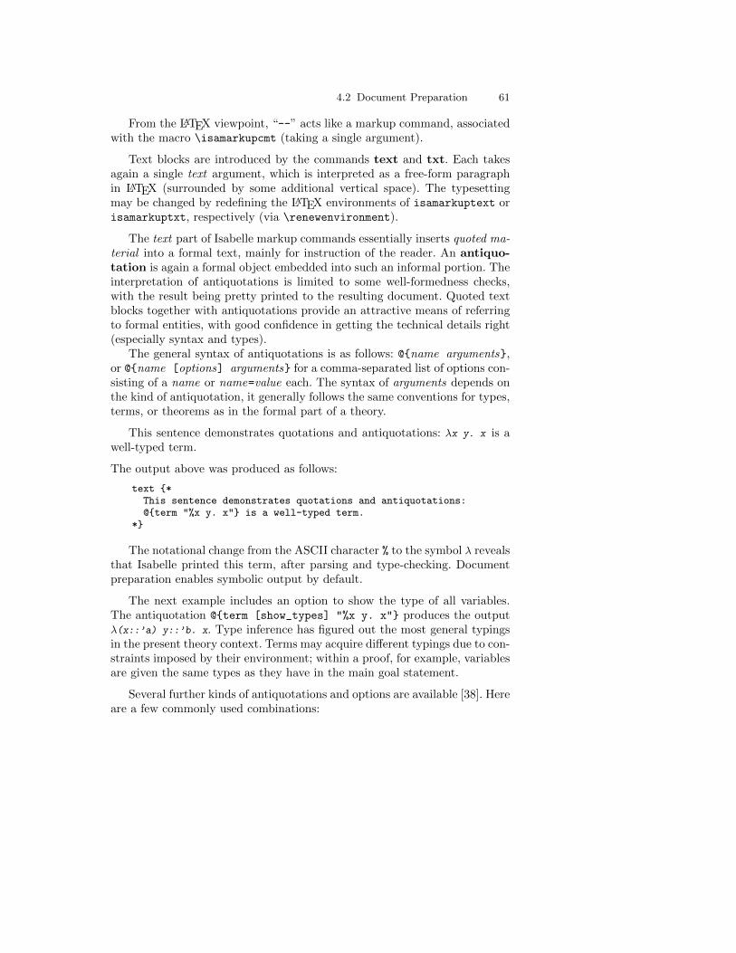
4.2 Document Preparation 61
From the LATEX viewpoint, “--” acts like a markup command, associatedwith the macro \isamarkupcmt (taking a single argument).
Text blocks are introduced by the commands text and txt. Each takesagain a single text argument, which is interpreted as a free-form paragraphin LATEX (surrounded by some additional vertical space). The typesettingmay be changed by redefining the LATEX environments of isamarkuptext orisamarkuptxt, respectively (via \renewenvironment).
The text part of Isabelle markup commands essentially inserts quoted ma-terial into a formal text, mainly for instruction of the reader. An antiquo-tation is again a formal object embedded into such an informal portion. Theinterpretation of antiquotations is limited to some well-formedness checks,with the result being pretty printed to the resulting document. Quoted textblocks together with antiquotations provide an attractive means of referringto formal entities, with good confidence in getting the technical details right(especially syntax and types).
The general syntax of antiquotations is as follows: @{name arguments},or @{name [options] arguments} for a comma-separated list of options con-sisting of a name or name=value each. The syntax of arguments depends onthe kind of antiquotation, it generally follows the same conventions for types,terms, or theorems as in the formal part of a theory.
This sentence demonstrates quotations and antiquotations: λx y. x is awell-typed term.
The output above was produced as follows:
text {*This sentence demonstrates quotations and antiquotations:@{term "%x y. x"} is a well-typed term.
*}
The notational change from the ASCII character % to the symbol λ revealsthat Isabelle printed this term, after parsing and type-checking. Documentpreparation enables symbolic output by default.
The next example includes an option to show the type of all variables.The antiquotation @{term [show_types] "%x y. x"} produces the outputλ(x::’a) y::’b. x. Type inference has figured out the most general typingsin the present theory context. Terms may acquire different typings due to con-straints imposed by their environment; within a proof, for example, variablesare given the same types as they have in the main goal statement.
Several further kinds of antiquotations and options are available [38]. Hereare a few commonly used combinations:
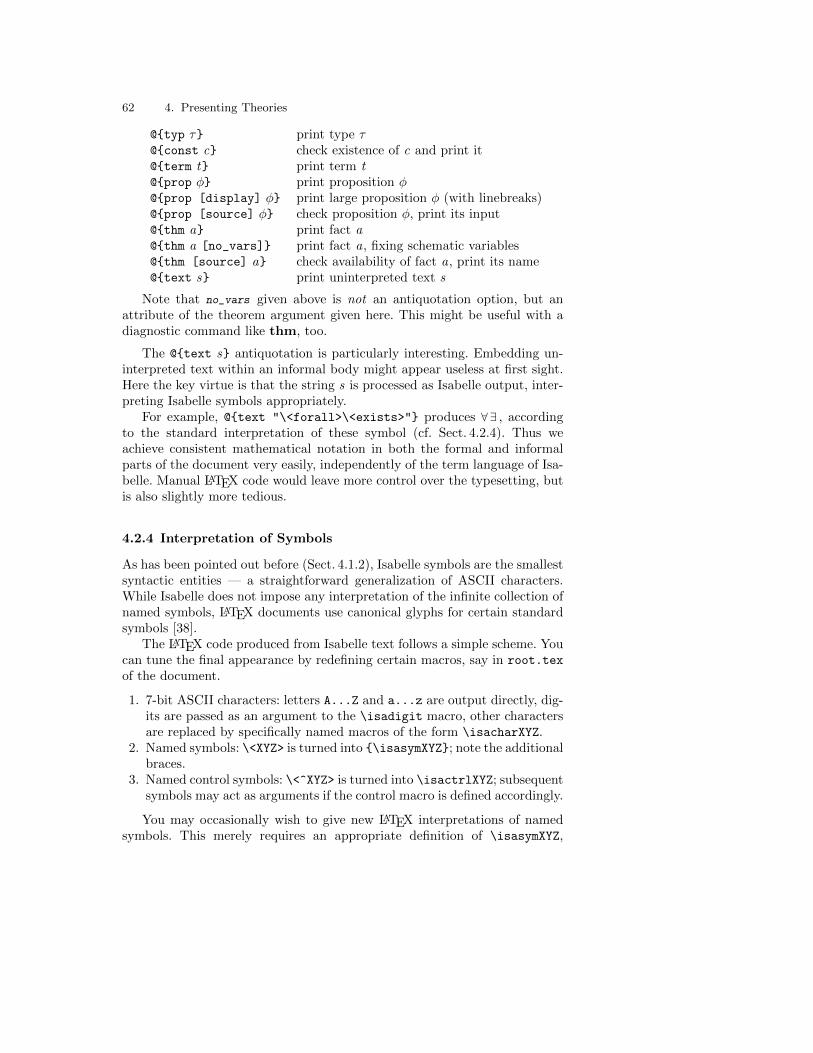
62 4. Presenting Theories
@{typ τ} print type τ@{const c} check existence of c and print it@{term t} print term t@{prop φ} print proposition φ@{prop [display] φ} print large proposition φ (with linebreaks)@{prop [source] φ} check proposition φ, print its input@{thm a} print fact a@{thm a [no_vars]} print fact a, fixing schematic variables@{thm [source] a} check availability of fact a, print its name@{text s} print uninterpreted text s
Note that no_vars given above is not an antiquotation option, but anattribute of the theorem argument given here. This might be useful with adiagnostic command like thm, too.
The @{text s} antiquotation is particularly interesting. Embedding un-interpreted text within an informal body might appear useless at first sight.Here the key virtue is that the string s is processed as Isabelle output, inter-preting Isabelle symbols appropriately.
For example, @{text "\<forall>\<exists>"} produces ∀∃ , accordingto the standard interpretation of these symbol (cf. Sect. 4.2.4). Thus weachieve consistent mathematical notation in both the formal and informalparts of the document very easily, independently of the term language of Isa-belle. Manual LATEX code would leave more control over the typesetting, butis also slightly more tedious.
4.2.4 Interpretation of Symbols
As has been pointed out before (Sect. 4.1.2), Isabelle symbols are the smallestsyntactic entities — a straightforward generalization of ASCII characters.While Isabelle does not impose any interpretation of the infinite collection ofnamed symbols, LATEX documents use canonical glyphs for certain standardsymbols [38].
The LATEX code produced from Isabelle text follows a simple scheme. Youcan tune the final appearance by redefining certain macros, say in root.tex
of the document.
1. 7-bit ASCII characters: letters A...Z and a...z are output directly, dig-its are passed as an argument to the \isadigit macro, other charactersare replaced by specifically named macros of the form \isacharXYZ.
2. Named symbols: \<XYZ> is turned into {\isasymXYZ}; note the additionalbraces.
3. Named control symbols: \<^XYZ> is turned into \isactrlXYZ; subsequentsymbols may act as arguments if the control macro is defined accordingly.
You may occasionally wish to give new LATEX interpretations of namedsymbols. This merely requires an appropriate definition of \isasymXYZ,
4.2 Document Preparation 63
for \<XYZ> (see isabelle.sty for working examples). Control symbols areslightly more difficult to get right, though.
The \isabellestyle macro provides a high-level interface to tune thegeneral appearance of individual symbols. For example, \isabellestyle{it}uses the italics text style to mimic the general appearance of the LATEX mathmode; double quotes are not printed at all. The resulting quality of type-setting is quite good, so this should be the default style for work that getsdistributed to a broader audience.
4.2.5 Suppressing Output
By default, Isabelle’s document system generates a LATEX file for each theorythat gets loaded while running the session. The generated session.tex willinclude all of these in order of appearance, which in turn gets included bythe standard root.tex. Certainly one may change the order or suppressunwanted theories by ignoring session.tex and load individual files directlyin root.tex. On the other hand, such an arrangement requires additionalmaintenance whenever the collection of theories changes.
Alternatively, one may tune the theory loading process in ROOT itself:some sequential order of theories sections may enforce a certain traversalof the dependency graph, although this could degrade parallel processing.The nodes of each sub-graph that is specified here are presented in sometopological order of their formal dependencies.
Moreover, the system build option document=false allows to disable doc-ument generation for some theories. Its usage in the session ROOT is like this:
theories [document = false] T
Theory output may be suppressed more selectively, either via taggedcommand regions or ignored material.
Tagged command regions works by annotating commands with namedtags, which correspond to certain LATEX markup that tells how to treat par-ticular parts of a document when doing the actual type-setting. By default,certain Isabelle/Isar commands are implicitly marked up using the predefinedtags “theory” (for theory begin and end), “proof ” (for proof commands), and“ML” (for commands involving ML code). Users may add their own tags us-ing the %tag notation right after a command name. In the subsequent examplewe hide a particularly irrelevant proof:
lemma "x = x"
The original source has been “lemma "x = x" by %invisible (simp)”.Tags observe the structure of proofs; adjacent commands with the same tagare joined into a single region. The Isabelle document preparation systemallows the user to specify how to interpret a tagged region, in order to keep,
64 4. Presenting Theories
drop, or fold the corresponding parts of the document. See the Isabelle SystemManual [37] for further details, especially on isabelle build and isabelle
document.Ignored material is specified by delimiting the original formal source with
special source comments (*<*) and (*>*). These parts are stripped beforethe type-setting phase, without affecting the formal checking of the theory, ofcourse. For example, we may hide parts of a proof that seem unfit for generalpublic inspection. The following “fully automatic” proof is actually a fake:
lemma "x 6= (0::int) =⇒ 0 < x * x"by (auto)
The real source of the proof has been as follows:
by (auto(*<*)simp add: zero_less_mult_iff(*>*))
Suppressing portions of printed text demands care. You should not mis-represent the underlying theory development. It is easy to invalidate thevisible text by hiding references to questionable axioms, for example.

Part II
Logic and Sets

5. The Rules of the Game
This chapter outlines the concepts and techniques that underlie reasoningin Isabelle. Until now, we have proved everything using only induction andsimplification, but any serious verification project requires more elaborateforms of inference. The chapter also introduces the fundamentals of predicatelogic. The first examples in this chapter will consist of detailed, low-level proofsteps. Later, we shall see how to automate such reasoning using the methodsblast, auto and others. Backward or goal-directed proof is our usual style,but the chapter also introduces forward reasoning, where one theorem istransformed to yield another.
5.1 Natural Deduction
In Isabelle, proofs are constructed using inference rules. The most familiarinference rule is probably modus ponens:
P → Q P
Q
This rule says that from P → Q and P we may infer Q .Natural deduction is an attempt to formalize logic in a way that mirrors
human reasoning patterns. For each logical symbol (say, ∧), there are twokinds of rules: introduction and elimination rules. The introduction rulesallow us to infer this symbol (say, to infer conjunctions). The eliminationrules allow us to deduce consequences from this symbol. Ideally each ruleshould mention one symbol only. For predicate logic this can be done, butwhen users define their own concepts they typically have to refer to othersymbols as well. It is best not to be dogmatic. Our system is not based onpure natural deduction, but includes elements from the sequent calculus andfree-variable tableaux.
Natural deduction generally deserves its name. It is easy to use. Each proofstep consists of identifying the outermost symbol of a formula and applyingthe corresponding rule. It creates new subgoals in an obvious way from partsof the chosen formula. Expanding the definitions of constants can blow upthe goal enormously. Deriving natural deduction rules for such constants
68 5. The Rules of the Game
lets us reason in terms of their key properties, which might otherwise beobscured by the technicalities of its definition. Natural deduction rules alsolend themselves to automation. Isabelle’s classical reasoner accepts anysuitable collection of natural deduction rules and uses them to search forproofs automatically. Isabelle is designed around natural deduction and manyof its tools use the terminology of introduction and elimination rules.
5.2 Introduction Rules
An introduction rule tells us when we can infer a formula containing a specificlogical symbol. For example, the conjunction introduction rule says that ifwe have P and if we have Q then we have P ∧Q . In a mathematics text, itis typically shown like this:
P Q
P ∧Q
The rule introduces the conjunction symbol (∧) in its conclusion. In Isabelleproofs we mainly reason backwards. When we apply this rule, the subgoalalready has the form of a conjunction; the proof step makes this conjunctionsymbol disappear.
In Isabelle notation, the rule looks like this:
[[?P; ?Q ]] =⇒ ?P ∧ ?Q (conjI)
Carefully examine the syntax. The premises appear to the left of the arrowand the conclusion to the right. The premises (if more than one) are groupedusing the fat brackets. The question marks indicate schematic variables(also called unknowns): they may be replaced by arbitrary formulas. If weuse the rule backwards, Isabelle tries to unify the current subgoal with theconclusion of the rule, which has the form ?P ∧ ?Q. (Unification is discussedbelow, Sect. 5.8.) If successful, it yields new subgoals given by the formulasassigned to ?P and ?Q.
The following trivial proof illustrates how rules work. It also introducesa style of indentation. If a command adds a new subgoal, then the nextcommand’s indentation is increased by one space; if it proves a subgoal, thenthe indentation is reduced. This provides the reader with hints about thesubgoal structure.
lemma conj_rule: " [[P; Q ]] =⇒ P ∧ (Q ∧ P)"apply (rule conjI)apply assumption
apply (rule conjI)apply assumption
apply assumption
At the start, Isabelle presents us with the assumptions (P and Q) and withthe goal to be proved, P ∧ (Q ∧ P). We are working backwards, so when we
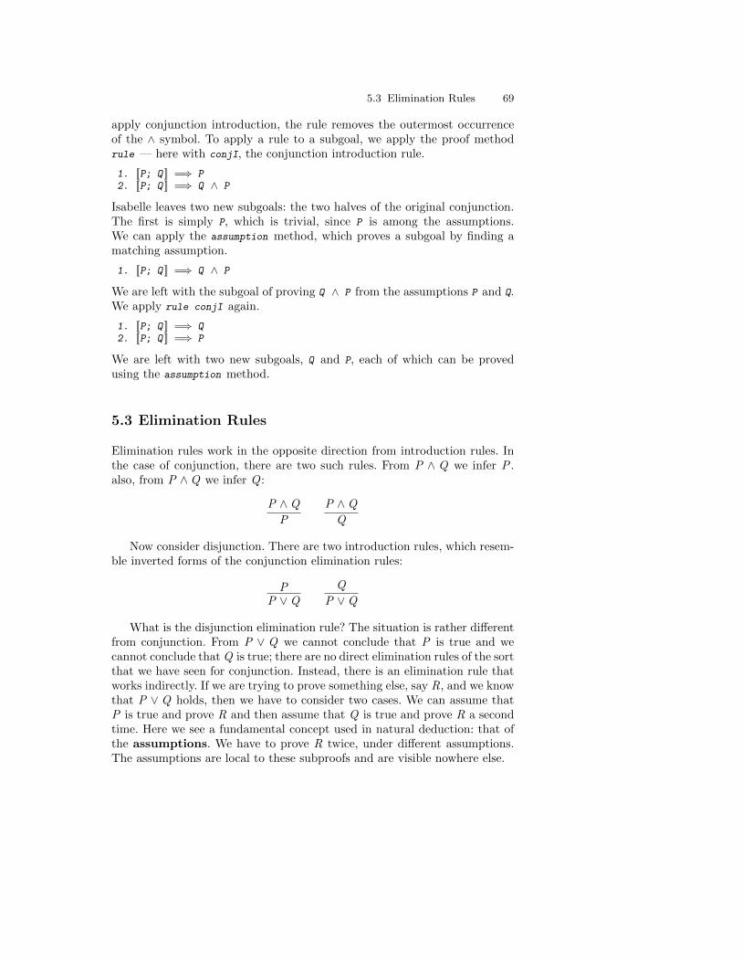
5.3 Elimination Rules 69
apply conjunction introduction, the rule removes the outermost occurrenceof the ∧ symbol. To apply a rule to a subgoal, we apply the proof methodrule — here with conjI, the conjunction introduction rule.
1. [[P; Q ]] =⇒ P2. [[P; Q ]] =⇒ Q ∧ P
Isabelle leaves two new subgoals: the two halves of the original conjunction.The first is simply P, which is trivial, since P is among the assumptions.We can apply the assumption method, which proves a subgoal by finding amatching assumption.
1. [[P; Q ]] =⇒ Q ∧ P
We are left with the subgoal of proving Q ∧ P from the assumptions P and Q.We apply rule conjI again.
1. [[P; Q ]] =⇒ Q2. [[P; Q ]] =⇒ P
We are left with two new subgoals, Q and P, each of which can be provedusing the assumption method.
5.3 Elimination Rules
Elimination rules work in the opposite direction from introduction rules. Inthe case of conjunction, there are two such rules. From P ∧ Q we infer P .also, from P ∧Q we infer Q :
P ∧Q
P
P ∧Q
Q
Now consider disjunction. There are two introduction rules, which resem-ble inverted forms of the conjunction elimination rules:
PP ∨Q
Q
P ∨Q
What is the disjunction elimination rule? The situation is rather differentfrom conjunction. From P ∨ Q we cannot conclude that P is true and wecannot conclude that Q is true; there are no direct elimination rules of the sortthat we have seen for conjunction. Instead, there is an elimination rule thatworks indirectly. If we are trying to prove something else, say R, and we knowthat P ∨ Q holds, then we have to consider two cases. We can assume thatP is true and prove R and then assume that Q is true and prove R a secondtime. Here we see a fundamental concept used in natural deduction: that ofthe assumptions. We have to prove R twice, under different assumptions.The assumptions are local to these subproofs and are visible nowhere else.
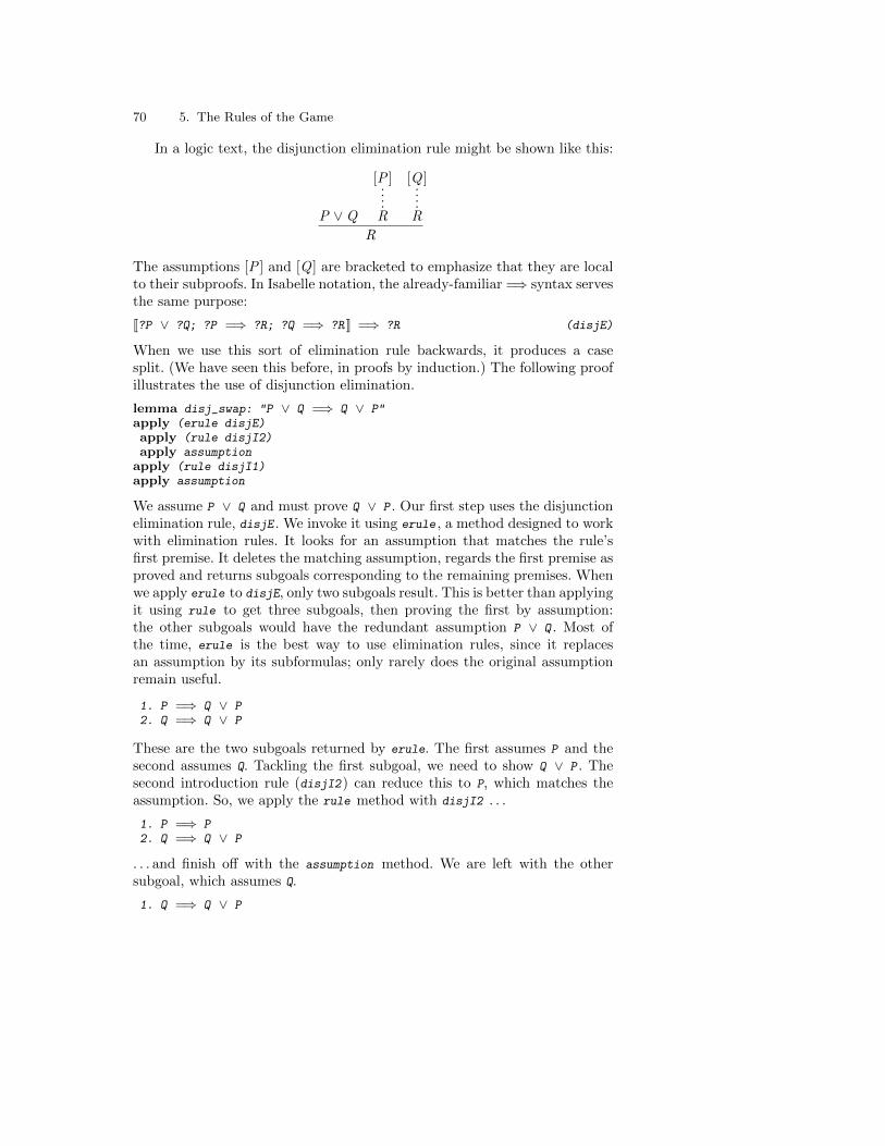
70 5. The Rules of the Game
In a logic text, the disjunction elimination rule might be shown like this:
P ∨Q
[P ]....R
[Q ]....R
R
The assumptions [P ] and [Q ] are bracketed to emphasize that they are localto their subproofs. In Isabelle notation, the already-familiar =⇒ syntax servesthe same purpose:
[[?P ∨ ?Q; ?P =⇒ ?R; ?Q =⇒ ?R ]] =⇒ ?R (disjE)
When we use this sort of elimination rule backwards, it produces a casesplit. (We have seen this before, in proofs by induction.) The following proofillustrates the use of disjunction elimination.
lemma disj_swap: "P ∨ Q =⇒ Q ∨ P"apply (erule disjE)apply (rule disjI2)apply assumption
apply (rule disjI1)apply assumption
We assume P ∨ Q and must prove Q ∨ P . Our first step uses the disjunctionelimination rule, disjE . We invoke it using erule , a method designed to workwith elimination rules. It looks for an assumption that matches the rule’sfirst premise. It deletes the matching assumption, regards the first premise asproved and returns subgoals corresponding to the remaining premises. Whenwe apply erule to disjE, only two subgoals result. This is better than applyingit using rule to get three subgoals, then proving the first by assumption:the other subgoals would have the redundant assumption P ∨ Q . Most ofthe time, erule is the best way to use elimination rules, since it replacesan assumption by its subformulas; only rarely does the original assumptionremain useful.
1. P =⇒ Q ∨ P2. Q =⇒ Q ∨ P
These are the two subgoals returned by erule. The first assumes P and thesecond assumes Q. Tackling the first subgoal, we need to show Q ∨ P . Thesecond introduction rule (disjI2) can reduce this to P, which matches theassumption. So, we apply the rule method with disjI2 . . .
1. P =⇒ P2. Q =⇒ Q ∨ P
. . . and finish off with the assumption method. We are left with the othersubgoal, which assumes Q.
1. Q =⇒ Q ∨ P
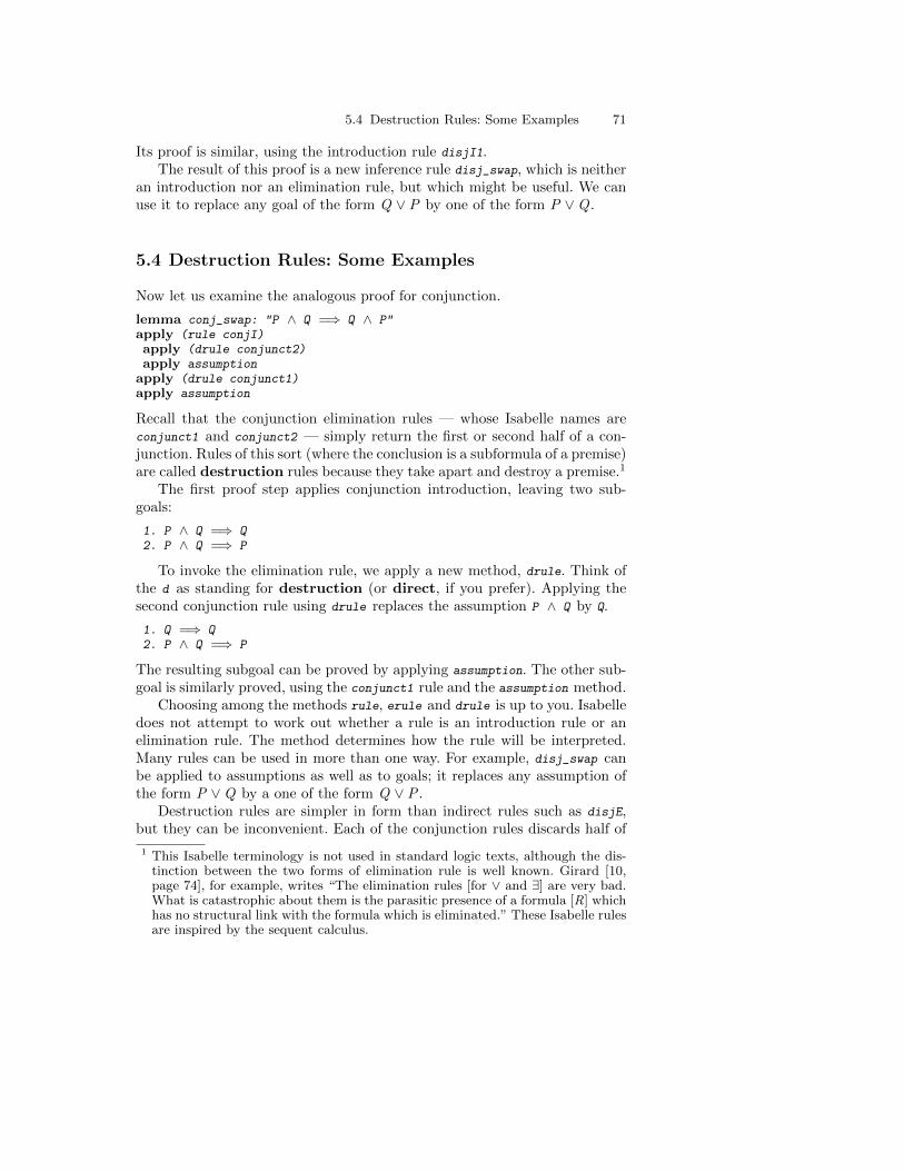
5.4 Destruction Rules: Some Examples 71
Its proof is similar, using the introduction rule disjI1.The result of this proof is a new inference rule disj_swap, which is neither
an introduction nor an elimination rule, but which might be useful. We canuse it to replace any goal of the form Q ∨ P by one of the form P ∨Q .
5.4 Destruction Rules: Some Examples
Now let us examine the analogous proof for conjunction.
lemma conj_swap: "P ∧ Q =⇒ Q ∧ P"apply (rule conjI)apply (drule conjunct2)apply assumption
apply (drule conjunct1)apply assumption
Recall that the conjunction elimination rules — whose Isabelle names areconjunct1 and conjunct2 — simply return the first or second half of a con-junction. Rules of this sort (where the conclusion is a subformula of a premise)are called destruction rules because they take apart and destroy a premise.1
The first proof step applies conjunction introduction, leaving two sub-goals:
1. P ∧ Q =⇒ Q2. P ∧ Q =⇒ P
To invoke the elimination rule, we apply a new method, drule. Think ofthe d as standing for destruction (or direct, if you prefer). Applying thesecond conjunction rule using drule replaces the assumption P ∧ Q by Q.
1. Q =⇒ Q2. P ∧ Q =⇒ P
The resulting subgoal can be proved by applying assumption. The other sub-goal is similarly proved, using the conjunct1 rule and the assumption method.
Choosing among the methods rule, erule and drule is up to you. Isabelledoes not attempt to work out whether a rule is an introduction rule or anelimination rule. The method determines how the rule will be interpreted.Many rules can be used in more than one way. For example, disj_swap canbe applied to assumptions as well as to goals; it replaces any assumption ofthe form P ∨Q by a one of the form Q ∨ P .
Destruction rules are simpler in form than indirect rules such as disjE,but they can be inconvenient. Each of the conjunction rules discards half of
1 This Isabelle terminology is not used in standard logic texts, although the dis-tinction between the two forms of elimination rule is well known. Girard [10,page 74], for example, writes “The elimination rules [for ∨ and ∃] are very bad.What is catastrophic about them is the parasitic presence of a formula [R] whichhas no structural link with the formula which is eliminated.” These Isabelle rulesare inspired by the sequent calculus.
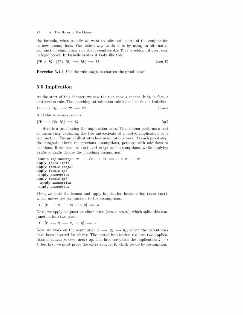
72 5. The Rules of the Game
the formula, when usually we want to take both parts of the conjunctionas new assumptions. The easiest way to do so is by using an alternativeconjunction elimination rule that resembles disjE . It is seldom, if ever, seenin logic books. In Isabelle syntax it looks like this:
[[?P ∧ ?Q; [[?P; ?Q ]] =⇒ ?R ]] =⇒ ?R (conjE)
Exercise 5.4.1 Use the rule conjE to shorten the proof above.
5.5 Implication
At the start of this chapter, we saw the rule modus ponens. It is, in fact, adestruction rule. The matching introduction rule looks like this in Isabelle:
(?P =⇒ ?Q) =⇒ ?P −→ ?Q (impI)
And this is modus ponens:
[[?P −→ ?Q; ?P ]] =⇒ ?Q (mp)
Here is a proof using the implication rules. This lemma performs a sortof uncurrying, replacing the two antecedents of a nested implication by aconjunction. The proof illustrates how assumptions work. At each proof step,the subgoals inherit the previous assumptions, perhaps with additions ordeletions. Rules such as impI and disjE add assumptions, while applyingerule or drule deletes the matching assumption.
lemma imp_uncurry: "P −→ (Q −→ R) =⇒ P ∧ Q −→ R"apply (rule impI)apply (erule conjE)apply (drule mp)apply assumption
apply (drule mp)apply assumption
apply assumption
First, we state the lemma and apply implication introduction (rule impI),which moves the conjunction to the assumptions.
1. [[P −→ Q −→ R; P ∧ Q ]] =⇒ R
Next, we apply conjunction elimination (erule conjE), which splits this con-junction into two parts.
1. [[P −→ Q −→ R; P; Q ]] =⇒ R
Now, we work on the assumption P −→ (Q −→ R), where the parentheseshave been inserted for clarity. The nested implication requires two applica-tions of modus ponens: drule mp. The first use yields the implication Q −→R, but first we must prove the extra subgoal P, which we do by assumption.
5.6 Negation 73
1. [[P; Q ]] =⇒ P2. [[P; Q; Q −→ R ]] =⇒ R
Repeating these steps for Q −→ R yields the conclusion we seek, namely R.
1. [[P; Q; Q −→ R ]] =⇒ R
The symbols =⇒ and −→ both stand for implication, but they differ inmany respects. Isabelle uses =⇒ to express inference rules; the symbol isbuilt-in and Isabelle’s inference mechanisms treat it specially. On the otherhand, −→ is just one of the many connectives available in higher-order logic.We reason about it using inference rules such as impI and mp, just as wereason about the other connectives. You will have to use −→ in any contextthat requires a formula of higher-order logic. Use =⇒ to separate a theorem’spreconditions from its conclusion.
The by command is useful for proofs like these that use assumption heav-ily. It executes an apply command, then tries to prove all remaining subgoalsusing assumption. Since (if successful) it ends the proof, it also replaces thedone symbol. For example, the proof above can be shortened:
lemma imp_uncurry: "P −→ (Q −→ R) =⇒ P ∧ Q −→ R"apply (rule impI)apply (erule conjE)apply (drule mp)apply assumption
by (drule mp)
We could use by to replace the final apply and done in any proof, buttypically we use it to eliminate calls to assumption. It is also a nice way ofexpressing a one-line proof.
5.6 Negation
Negation causes surprising complexity in proofs. Its natural deduction rulesare straightforward, but additional rules seem necessary in order to han-dle negated assumptions gracefully. This section also illustrates the intro
method: a convenient way of applying introduction rules.Negation introduction deduces ¬P if assuming P leads to a contradiction.
Negation elimination deduces any formula in the presence of ¬P togetherwith P :
(?P =⇒ False) =⇒ ¬ ?P (notI)[[¬ ?P; ?P ]] =⇒ ?R (notE)
Classical logic allows us to assume ¬P when attempting to prove P :
(¬ ?P =⇒ ?P) =⇒ ?P (classical)
74 5. The Rules of the Game
The implications P → Q and ¬Q → ¬P are logically equivalent, andeach is called the contrapositive of the other. Four further rules supportreasoning about contrapositives. They differ in the placement of the negationsymbols:
[[?Q; ¬ ?P =⇒ ¬ ?Q ]] =⇒ ?P (contrapos_pp)[[?Q; ?P =⇒ ¬ ?Q ]] =⇒ ¬ ?P (contrapos_pn)[[¬ ?Q; ¬ ?P =⇒ ?Q ]] =⇒ ?P (contrapos_np)[[¬ ?Q; ?P =⇒ ?Q ]] =⇒ ¬ ?P (contrapos_nn)
These rules are typically applied using the erule method, where their effectis to form a contrapositive from an assumption and the goal’s conclusion.
The most important of these is contrapos_np. It is useful for applyingintroduction rules to negated assumptions. For instance, the assumption¬(P → Q) is equivalent to the conclusion P → Q and we might want touse conjunction introduction on it. Before we can do so, we must move thatassumption so that it becomes the conclusion. The following proof demon-strates this technique:
lemma " [[¬(P−→Q); ¬(R−→Q) ]] =⇒ R"apply (erule_tac Q = "R−→Q" in contrapos_np)apply (intro impI)by (erule notE)
There are two negated assumptions and we need to exchange the conclusionwith the second one. The method erule contrapos_np would select the firstassumption, which we do not want. So we specify the desired assumptionexplicitly using a new method, erule_tac. This is the resulting subgoal:
1. [[¬ (P −→ Q); ¬ R ]] =⇒ R −→ Q
The former conclusion, namely R, now appears negated among the assump-tions, while the negated formula R −→ Q becomes the new conclusion.
We can now apply introduction rules. We use the intro method, whichrepeatedly applies the given introduction rules. Here its effect is equivalentto rule impI.
1. [[¬ (P −→ Q); ¬ R; R ]] =⇒ Q
We can see a contradiction in the form of assumptions ¬ R and R, whichsuggests using negation elimination. If applied on its own, notE will selectthe first negated assumption, which is useless. Instead, we invoke the ruleusing the by command. Now when Isabelle selects the first assumption, ittries to prove P −→ Q and fails; it then backtracks, finds the assumption ¬ R
and finally proves R by assumption. That concludes the proof.
The following example may be skipped on a first reading. It involves apeculiar but important rule, a form of disjunction introduction:
(¬ ?Q =⇒ ?P) =⇒ ?P ∨ ?Q (disjCI)
5.7 Interlude: the Basic Methods for Rules 75
This rule combines the effects of disjI1 and disjI2. Its great advantageis that we can remove the disjunction symbol without deciding which dis-junction to prove. This treatment of disjunction is standard in sequent andtableau calculi.
lemma "(P ∨ Q) ∧ R =⇒ P ∨ (Q ∧ R)"apply (rule disjCI)apply (elim conjE disjE)apply assumption
by (erule contrapos_np, rule conjI)
The first proof step to applies the introduction rules disjCI. The resultingsubgoal has the negative assumption ¬(Q ∧ R) .
1. [[(P ∨ Q) ∧ R; ¬ (Q ∧ R) ]] =⇒ P
Next we apply the elim method, which repeatedly applies elimination rules;here, the elimination rules given in the command. One of the subgoals istrivial (apply assumption), leaving us with one other:
1. [[¬ (Q ∧ R); R; Q ]] =⇒ P
Now we must move the formula Q ∧ R to be the conclusion. The combination
(erule contrapos_np, rule conjI)
is robust: the conjI forces the erule to select a conjunction. The two subgoalsare the ones we would expect from applying conjunction introduction toQ ∧ R :
1. [[R; Q; ¬ P ]] =⇒ Q2. [[R; Q; ¬ P ]] =⇒ R
They are proved by assumption, which is implicit in the by command.
5.7 Interlude: the Basic Methods for Rules
We have seen examples of many tactics that operate on individual rules. Itmay be helpful to review how they work given an arbitrary rule such as this:
P1 . . . Pn
Q
Below, we refer to P1 as the major premise. This concept applies only toelimination and destruction rules. These rules act upon an instance of theirmajor premise, typically to replace it by subformulas of itself.
Suppose that the rule above is called R . Here are the basic rule methods,most of which we have already seen:
– Method rule R unifies Q with the current subgoal, replacing it by n newsubgoals: instances of P1, . . . , Pn . This is backward reasoning and is ap-propriate for introduction rules.
76 5. The Rules of the Game
– Method erule R unifies Q with the current subgoal and simultaneouslyunifies P1 with some assumption. The subgoal is replaced by the n−1 newsubgoals of proving instances of P2, . . . , Pn , with the matching assump-tion deleted. It is appropriate for elimination rules. The method (rule R,
assumption) is similar, but it does not delete an assumption.– Method drule R unifies P1 with some assumption, which it then deletes.
The subgoal is replaced by the n − 1 new subgoals of proving P2, . . . , Pn ;an nth subgoal is like the original one but has an additional assumption:an instance of Q . It is appropriate for destruction rules.
– Method frule R is like drule R except that the matching assumption isnot deleted. (See Sect. 5.9.5 below.)
Other methods apply a rule while constraining some of its variables. Thetypical form is
rule_tac v1 = t1 and ...and vk = tk in R
This method behaves like rule R, while instantiating the variables v1, . . . , vkas specified. We similarly have erule_tac , drule_tac and frule_tac . Thesemethods also let us specify which subgoal to operate on. By default it isthe first subgoal, as with nearly all methods, but we can specify that rule R
should be applied to subgoal number i :
rule_tac [i] R
5.8 Unification and Substitution
As we have seen, Isabelle rules involve schematic variables, which begin with aquestion mark and act as placeholders for terms. Unification — well knownto Prolog programmers — is the act of making two terms identical, possi-bly replacing their schematic variables by terms. The simplest case is whenthe two terms are already the same. Next simplest is pattern-matching,which replaces variables in only one of the terms. The rule method typicallymatches the rule’s conclusion against the current subgoal. The assumption
method matches the current subgoal’s conclusion against each of its assump-tions. Unification can instantiate variables in both terms; the rule methodcan do this if the goal itself contains schematic variables. Other occurrencesof the variables in the rule or proof state are updated at the same time.
Schematic variables in goals represent unknown terms. Given a goal suchas ∃x .P , they let us proceed with a proof. They can be filled in later, some-times in stages and often automatically.
If unification fails when you think it should succeed, try setting the Proof Gen-eral flag Isabelle > Settings > Trace Unification, which makes Isabelle show the
cause of unification failures (in Proof General’s Trace buffer).
5.8 Unification and Substitution 77
For example, suppose we are trying to prove this subgoal by assumption:
1. P (a, f (b, g (e, a), b), a) =⇒ P (a, f (b, g (c, a), b), a)
The assumption method having failed, we try again with the flag set:
apply assumption
In this trivial case, the output clearly shows that e clashes with c :
Clash: e =/= c
Isabelle uses higher-order unification, which works in the typed λ-calculus. The procedure requires search and is potentially undecidable. Forour purposes, however, the differences from ordinary unification are straight-forward. It handles bound variables correctly, avoiding capture. The twoterms λx. f(x,z) and λy. f(y,z) are trivially unifiable because they dif-fer only by a bound variable renaming. The two terms λx. ?P and λx. t x
are not unifiable; replacing ?P by t x is forbidden because the free occur-rence of x would become bound. Unfortunately, even if trace_unify_fail isset, Isabelle displays no information about this type of failure.
!! Higher-order unification sometimes must invent λ-terms to replace functionvariables, which can lead to a combinatorial explosion. However, Isabelle proofs
tend to involve easy cases where there are few possibilities for the λ-term beingconstructed. In the easiest case, the function variable is applied only to boundvariables, as when we try to unify λx y. f(?h x y) and λx y. f(x+y+a). Theonly solution is to replace ?h by λx y. x+y+a. Such cases admit at most one unifier,like ordinary unification. A harder case is unifying ?h a with a+b ; it admits twosolutions for ?h, namely λx. a+b and λx. x+b. Unifying ?h a with a+a+b admitsfour solutions; their number is exponential in the number of occurrences of a in thesecond term.
5.8.1 Substitution and the subst Method
Isabelle also uses function variables to express substitution. A typical sub-stitution rule allows us to replace one term by another if we know that twoterms are equal.
s = t P [s/x ]
P [t/x ]
The rule uses a notation for substitution: P [t/x ] is the result of replacing xby t in P . The rule only substitutes in the positions designated by x . Forexample, it can derive symmetry of equality from reflexivity. Using x = sfor P replaces just the first s in s = s by t :
s = t s = st = s
The Isabelle version of the substitution rule looks like this:
78 5. The Rules of the Game
[[?t = ?s; ?P ?s ]] =⇒ ?P ?t (ssubst)
Crucially, ?P is a function variable. It can be replaced by a λ-term withone bound variable, whose occurrences identify the places in which s will bereplaced by t . The proof above requires ?P to be replaced by λx. x=s ; thesecond premise will then be s=s and the conclusion will be t=s.
The simp method also replaces equals by equals, but the substitution rulegives us more control. Consider this proof:
lemma " [[x = f x; odd(f x) ]] =⇒ odd x"by (erule ssubst)
The assumption x = f x, if used for rewriting, would loop, replacing x by f x
and then by f(f x) and so forth. (Here simp would see the danger and wouldre-orient the equality, but in more complicated cases it can be fooled.) Whenwe apply the substitution rule, Isabelle replaces every x in the subgoal by f
x just once. It cannot loop. The resulting subgoal is trivial by assumption,so the by command proves it implicitly.
We are using the erule method in a novel way. Hitherto, the conclusion ofthe rule was just a variable such as ?R, but it may be any term. The conclusionis unified with the subgoal just as it would be with the rule method. Atthe same time erule looks for an assumption that matches the rule’s firstpremise, as usual. With ssubst the effect is to find, use and delete an equalityassumption.
The subst method performs individual substitutions. In simple cases, itclosely resembles a use of the substitution rule. Suppose a proof has reachedthis point:
1. [[P x y z; Suc x < y ]] =⇒ f z = x * y
Now we wish to apply a commutative law:
?m * ?n = ?n * ?m (mult.commute)
Isabelle rejects our first attempt:
apply (simp add: mult.commute)
The simplifier notices the danger of looping and refuses to apply the rule.2
The subst method applies mult.commute exactly once.
apply (subst mult.commute)1. [[P x y z; Suc x < y ]] =⇒ f z = y * x
As we wanted, x * y has become y * x.
This use of the subst method has the same effect as the command
apply (rule mult.commute [THEN ssubst])
2 More precisely, it only applies such a rule if the new term is smaller under aspecified ordering; here, x * y is already smaller than y * x.
5.8 Unification and Substitution 79
The attribute THEN, which combines two rules, is described in Sect. 5.15.1 be-low. The subst method is more powerful than applying the substitution rule.It can perform substitutions in a subgoal’s assumptions. Moreover, if the sub-goal contains more than one occurrence of the left-hand side of the equality,the subst method lets us specify which occurrence should be replaced.
5.8.2 Unification and Its Pitfalls
Higher-order unification can be tricky. Here is an example, which you maywant to skip on your first reading:
lemma " [[x = f x; triple (f x) (f x) x ]] =⇒ triple x x x"apply (erule ssubst)backbackbackbackapply assumptiondone
By default, Isabelle tries to substitute for all the occurrences. Applying erule
ssubst yields this subgoal:
1. triple (f x) (f x) x =⇒ triple (f x) (f x) (f x)
The substitution should have been done in the first two occurrences of x
only. Isabelle has gone too far. The back command allows us to reject thispossibility and demand a new one:
1. triple (f x) (f x) x =⇒ triple x (f x) (f x)
Now Isabelle has left the first occurrence of x alone. That is promising butit is not the desired combination. So we use back again:
1. triple (f x) (f x) x =⇒ triple (f x) x (f x)
This also is wrong, so we use back again:
1. triple (f x) (f x) x =⇒ triple x x (f x)
And this one is wrong too. Looking carefully at the series of alternatives, wesee a binary countdown with reversed bits: 111, 011, 101, 001. Invoke backagain:
1. triple (f x) (f x) x =⇒ triple (f x) (f x) x
At last, we have the right combination! This goal follows by assumption.
This example shows that unification can do strange things with functionvariables. We were forced to select the right unifier using the back command.That is all right during exploration, but back should never appear in the finalversion of a proof. You can eliminate the need for back by giving Isabelleless freedom when you apply a rule.
80 5. The Rules of the Game
One way to constrain the inference is by joining two methods in a applycommand. Isabelle applies the first method and then the second. If the secondmethod fails then Isabelle automatically backtracks. This process continuesuntil the first method produces an output that the second method can use.We get a one-line proof of our example:
lemma " [[x = f x; triple (f x) (f x) x ]] =⇒ triple x x x"apply (erule ssubst, assumption)done
The by command works too, since it backtracks when proving subgoals byassumption:
lemma " [[x = f x; triple (f x) (f x) x ]] =⇒ triple x x x"by (erule ssubst)
The most general way to constrain unification is by instantiating variablesin the rule. The method rule_tac is similar to rule, but it makes some ofthe rule’s variables denote specified terms. Also available are drule_tac anderule_tac. Here we need erule_tac since above we used erule.
lemma " [[x = f x; triple (f x) (f x) x ]] =⇒ triple x x x"by (erule_tac P = "λu. triple u u x" in ssubst)
To specify a desired substitution requires instantiating the variable ?P witha λ-expression. The bound variable occurrences in λu. P u u x indicate thatthe first two arguments have to be substituted, leaving the third unchanged.With this instantiation, backtracking is neither necessary nor possible.
An alternative to rule_tac is to use rule with a theorem modified us-ing of, described in Sect. 5.15 below. But rule_tac, unlike of, can expressinstantiations that refer to
∧-bound variables in the current subgoal.
5.9 Quantifiers
Quantifiers require formalizing syntactic substitution and the notion of arbi-trary value. Consider the universal quantifier. In a logic book, its introductionrule looks like this:
P∀x .P
Typically, a proviso written in English says that x must not occur in the as-sumptions. This proviso guarantees that x can be regarded as arbitrary, sinceit has not been assumed to satisfy any special conditions. Isabelle’s under-lying formalism, called the meta-logic, eliminates the need for English. Itprovides its own universal quantifier (
∧) to express the notion of an arbitrary
value. We have already seen another operator of the meta-logic, namely =⇒,which expresses inference rules and the treatment of assumptions. The onlyother operator in the meta-logic is ≡, which can be used to define constants.
5.9 Quantifiers 81
5.9.1 The Universal Introduction Rule
Returning to the universal quantifier, we find that having a similar quantifieras part of the meta-logic makes the introduction rule trivial to express:
(∧x. ?P x) =⇒ ∀ x. ?P x (allI)
The following trivial proof demonstrates how the universal introductionrule works.
lemma "∀ x. P x −→ P x"apply (rule allI)by (rule impI)
The first step invokes the rule by applying the method rule allI.
1.∧x. P x −→ P x
Note that the resulting proof state has a bound variable, namely x. The rulehas replaced the universal quantifier of higher-order logic by Isabelle’s meta-level quantifier. Our goal is to prove P x −→ P x for arbitrary x ; it is animplication, so we apply the corresponding introduction rule (impI).
1.∧x. P x =⇒ P x
This last subgoal is implicitly proved by assumption.
5.9.2 The Universal Elimination Rule
Now consider universal elimination. In a logic text, the rule looks like this:
∀x .PP [t/x ]
The conclusion is P with t substituted for the variable x . Isabelle expressessubstitution using a function variable:
∀ x. ?P x =⇒ ?P ?x (spec)
This destruction rule takes a universally quantified formula and removes thequantifier, replacing the bound variable x by the schematic variable ?x. Re-call that a schematic variable starts with a question mark and acts as aplaceholder: it can be replaced by any term.
The universal elimination rule is also available in the standard eliminationformat. Like conjE, it never appears in logic books:
[[∀ x. ?P x; ?P ?x =⇒ ?R ]] =⇒ ?R (allE)
The methods drule spec and erule allE do precisely the same inference.To see how ∀-elimination works, let us derive a rule about reducing the
scope of a universal quantifier. In mathematical notation we write
∀x .P → Q
P → ∀x .Q
82 5. The Rules of the Game
with the proviso “x not free in P .” Isabelle’s treatment of substitution makesthe proviso unnecessary. The conclusion is expressed as P −→ (∀ x. Q x).No substitution for the variable P can introduce a dependence upon x : thatwould be a bound variable capture. Let us walk through the proof.
lemma "(∀ x. P −→ Q x) =⇒ P −→ (∀ x. Q x)"
First we apply implies introduction (impI), which moves the P from the con-clusion to the assumptions. Then we apply universal introduction (allI).
apply (rule impI, rule allI)1.
∧x. [[∀ x. P −→ Q x; P ]] =⇒ Q x
As before, it replaces the HOL quantifier by a meta-level quantifier, producinga subgoal that binds the variable x. The leading bound variables (here x)and the assumptions (here ∀ x. P −→ Q x and P) form the context for theconclusion, here Q x. Subgoals inherit the context, although assumptions canbe added or deleted (as we saw earlier), while rules such as allI add boundvariables.
Now, to reason from the universally quantified assumption, we apply theelimination rule using the drule method. This rule is called spec because itspecializes a universal formula to a particular term.
apply (drule spec)1.
∧x. [[P; P −→ Q (?x2 x) ]] =⇒ Q x
Observe how the context has changed. The quantified formula is gone, re-placed by a new assumption derived from its body. We have removed thequantifier and replaced the bound variable by the curious term ?x2 x. Thisterm is a placeholder: it may become any term that can be built from x.(Formally, ?x2 is an unknown of function type, applied to the argument x.)This new assumption is an implication, so we can use modus ponens on it,which concludes the proof.
by (drule mp)
Let us take a closer look at this last step. Modus ponens yields two subgoals:one where we prove the antecedent (in this case P) and one where we mayassume the consequent. Both of these subgoals are proved by the assumption
method, which is implicit in the by command. Replacing the by commandby apply (drule mp, assumption) would have left one last subgoal:
1.∧x. [[P; Q (?x2 x) ]] =⇒ Q x
The consequent is Q applied to that placeholder. It may be replaced by anyterm built from x, and here it should simply be x. The assumption need notbe identical to the conclusion, provided the two formulas are unifiable.
5.9.3 The Existential Quantifier
The concepts just presented also apply to the existential quantifier, whoseintroduction rule looks like this in Isabelle:
5.9 Quantifiers 83
?P ?x =⇒ ∃ x. ?P x (exI)
If we can exhibit some x such that P(x ) is true, then ∃x .P(x ) is also true.It is a dual of the universal elimination rule, and logic texts present it usingthe same notation for substitution.
The existential elimination rule looks like this in a logic text:
∃x .P
[P ]....
Q
Q
It looks like this in Isabelle:
[[∃ x. ?P x;∧x. ?P x =⇒ ?Q ]] =⇒ ?Q (exE)
Given an existentially quantified theorem and some formula Q to prove, itcreates a new assumption by removing the quantifier. As with the universalintroduction rule, the textbook version imposes a proviso on the quantifiedvariable, which Isabelle expresses using its meta-logic. It is enough to have auniversal quantifier in the meta-logic; we do not need an existential quantifierto be built in as well.
Exercise 5.9.1 Prove the lemma
∃x .P ∧Q(x ) =⇒ P ∧ (∃x .Q(x )).
Hint : the proof is similar to the one just above for the universal quantifier.
5.9.4 Renaming a Bound Variable: rename_tac
When you apply a rule such as allI, the quantified variable becomes a newbound variable of the new subgoal. Isabelle tries to avoid changing its name,but sometimes it has to choose a new name in order to avoid a clash. Theresult may not be ideal:
lemma "x < y =⇒ ∀ x y. P x (f y)"apply (intro allI)1.
∧xa ya. x < y =⇒ P xa (f ya)
The names x and y were already in use, so the new bound variables are calledxa and ya. You can rename them by invoking rename_tac :
apply (rename_tac v w)1.
∧v w. x < y =⇒ P v (f w)
Recall that rule_tac instantiates a theorem with specified terms. These termsmay involve the goal’s bound variables, but beware of referring to variableslike xa. A future change to your theories could change the set of names pro-duced at top level, so that xa changes to xb or reverts to x. It is safer torename automatically-generated variables before mentioning them.
If the subgoal has more bound variables than there are names given torename_tac, the rightmost ones are renamed.
84 5. The Rules of the Game
5.9.5 Reusing an Assumption: frule
Note that drule spec removes the universal quantifier and — as usual withelimination rules — discards the original formula. Sometimes, a universalformula has to be kept so that it can be used again. Then we use a newmethod: frule. It acts like drule but copies rather than replaces the selectedassumption. The f is for forward.
In this example, going from P a to P(h(h a)) requires two uses of thequantified assumption, one for each h in h(h a).
lemma " [[∀ x. P x −→ P (h x); P a ]] =⇒ P(h (h a))"
Examine the subgoal left by frule :
apply (frule spec)1. [[∀ x. P x −→ P (h x); P a; P ?x −→ P (h ?x) ]] =⇒ P (h (h a))
It is what drule would have left except that the quantified assumption is stillpresent. Next we apply mp to the implication and the assumption P a :
apply (drule mp, assumption)1. [[∀ x. P x −→ P (h x); P a; P (h a) ]] =⇒ P (h (h a))
We have created the assumption P(h a), which is progress. To continue theproof, we apply spec again. We shall not need it again, so we can use drule.
apply (drule spec)1. [[P a; P (h a); P ?x2 −→ P (h ?x2) ]] =⇒ P (h (h a))
The new assumption bridges the gap between P(h a) and P(h(h a)).
by (drule mp)
A final remark. Replacing this by command with
apply (drule mp, assumption)
would not work: it would add a second copy of P(h a) instead of the desiredassumption, P(h(h a)). The by command forces Isabelle to backtrack until itfinds the correct one. Alternatively, we could have used the apply commandand bundled the drule mp with two calls of assumption. Or, of course, wecould have given the entire proof to auto.
5.9.6 Instantiating a Quantifier Explicitly
We can prove a theorem of the form ∃x .P x by exhibiting a suitable term tsuch that P t is true. Dually, we can use an assumption of the form ∀x .P x togenerate a new assumption P t for a suitable term t . In many cases, Isabellemakes the correct choice automatically, constructing the term by unification.In other cases, the required term is not obvious and we must specify it our-selves. Suitable methods are rule_tac, drule_tac and erule_tac.
We have seen (just above, Sect. 5.9.5) a proof of this lemma:
5.9 Quantifiers 85
lemma " [[∀ x. P x −→ P (h x); P a ]] =⇒ P(h (h a))"
We had reached this subgoal:
1. [[∀ x. P x −→ P (h x); P a; P (h a) ]] =⇒ P (h (h a))
The proof requires instantiating the quantified assumption with the term h a.
apply (drule_tac x = "h a" in spec)1. [[P a; P (h a); P (h a) −→ P (h (h a)) ]] =⇒ P (h (h a))
We have forced the desired instantiation.
Existential formulas can be instantiated too. The next example uses thedivides relation of number theory:
?m dvd ?n ≡ ∃ k. ?n = ?m * k (dvd_def)
Let us prove that multiplication of natural numbers is monotone withrespect to the divides relation:
lemma mult_dvd_mono: " [[i dvd m; j dvd n ]] =⇒ i*j dvd (m*n :: nat)"apply (simp add: dvd_def)
Unfolding the definition of divides has left this subgoal:
1. [[∃ k. m = i * k; ∃ k. n = j * k ]] =⇒ ∃ k. m * n = i * j * k
Next, we eliminate the two existential quantifiers in the assumptions:
apply (erule exE)1.
∧k. [[∃ k. n = j * k; m = i * k ]] =⇒ ∃ k. m * n = i * j * k
apply (erule exE)1.
∧k ka. [[m = i * k; n = j * ka ]] =⇒ ∃ k. m * n = i * j * k
The term needed to instantiate the remaining quantifier is k*ka. But ka is anautomatically-generated name. As noted above, references to such variablenames makes a proof less resilient to future changes. So, first we rename themost recent variable to l :
apply (rename_tac l)1.
∧k l. [[m = i * k; n = j * l ]] =⇒ ∃ k. m * n = i * j * k
We instantiate the quantifier with k*l :
apply (rule_tac x="k*l" in exI)1.
∧k ka. [[m = i * k; n = j * ka ]] =⇒ m * n = i * j * (k * ka)
The rest is automatic, by arithmetic.
apply simpdone
86 5. The Rules of the Game
5.10 Description Operators
HOL provides two description operators. A definite description formalizesthe word “the,” as in “the greatest divisior of n.” It returns an arbitraryvalue unless the formula has a unique solution. An indefinite descriptionformalizes the word “some,” as in “some member of S .” It differs from adefinite description in not requiring the solution to be unique: it uses theaxiom of choice to pick any solution.
!! Description operators can be hard to reason about. Novices should try to avoidthem. Fortunately, descriptions are seldom required.
5.10.1 Definite Descriptions
A definite description is traditionally written ιx .P(x ). It denotes the x suchthat P(x ) is true, provided there exists a unique such x ; otherwise, it re-turns an arbitrary value of the expected type. Isabelle uses THE for the Greekletter ι.
We reason using this rule, where a is the unique solution:
[[P a;∧x. P x =⇒ x = a ]] =⇒ (THE x. P x) = a (the_equality)
For instance, we can define the cardinality of a finite set A to be that nsuch that A is in one-to-one correspondence with {1, . . . ,n}. We can thenprove that the cardinality of the empty set is zero (since n = 0 satisfies thedescription) and proceed to prove other facts.
A more challenging example illustrates how Isabelle/HOL defines the leastnumber operator, which denotes the least x satisfying P :
(LEAST x. P x) = (THE x. P x ∧ (∀ y. P y −→ x ≤ y))
Let us prove the analogue of the_equality for LEAST .
theorem Least_equality:" [[P (k::nat); ∀ x. P x −→ k ≤ x ]] =⇒ (LEAST x. P x) = k"
apply (simp add: Least_def)
1. [[P k; ∀ x. P x −→ k ≤ x ]]=⇒ (THE x. P x ∧ (∀ y. P y −→ x ≤ y)) = k
The first step has merely unfolded the definition.
apply (rule the_equality)
1. [[P k; ∀ x. P x −→ k ≤ x ]] =⇒ P k ∧ (∀ y. P y −→ k ≤ y)2.
∧x. [[P k; ∀ x. P x −→ k ≤ x; P x ∧ (∀ y. P y −→ x ≤ y) ]]
=⇒ x = k
As always with the_equality, we must show existence and uniqueness of theclaimed solution, k. Existence, the first subgoal, is trivial. Uniqueness, thesecond subgoal, follows by antisymmetry:
5.10 Description Operators 87
[[x ≤ y; y ≤ x ]] =⇒ x = y (order_antisym)
The assumptions imply both k ≤ x and x ≤ k. One call to auto does it all:
by (auto intro: order_antisym)
5.10.2 Indefinite Descriptions
An indefinite description is traditionally written εx .P(x ) and is known asHilbert’s ε-operator. It denotes some x such that P(x ) is true, provided oneexists. Isabelle uses SOME for the Greek letter ε.
Here is the definition of inv ,3 which expresses inverses of functions:
inv f ≡ λy. SOME x. f x = y (inv_def)
Using SOME rather than THE makes inv f behave well even if f is not injective.As it happens, most useful theorems about inv do assume the function to beinjective.
The inverse of f, when applied to y, returns some x such that f x = y.For example, we can prove inv Suc really is the inverse of the Suc function
lemma "inv Suc (Suc n) = n"by (simp add: inv_def)
The proof is a one-liner: the subgoal simplifies to a degenerate application ofSOME, which is then erased. In detail, the left-hand side simplifies to SOME x.
Suc x = Suc n, then to SOME x. x = n and finally to n.We know nothing about what inv Suc returns when applied to zero. The
proof above still treats SOME as a definite description, since it only reasonsabout situations in which the value is described uniquely. Indeed, SOME satis-fies this rule:
[[P a;∧x. P x =⇒ x = a ]] =⇒ (SOME x. P x) = a (some_equality)
To go further is tricky and requires rules such as these:
P x =⇒ P (SOME x. P x) (someI)[[P a;
∧x. P x =⇒ Q x ]] =⇒ Q (SOME x. P x) (someI2)
Rule someI is basic: if anything satisfies P then so does SOME x. P x . Therepetition of P in the conclusion makes it difficult to apply in a backwardproof, so the derived rule someI2 is also provided.
For example, let us prove the axiom of choice:
theorem axiom_of_choice: "(∀ x. ∃ y. P x y) =⇒ ∃ f. ∀ x. P x (f x)"apply (rule exI, rule allI)
1.∧x. ∀ x. ∃ y. P x y =⇒ P x (?f x)
We have applied the introduction rules; now it is time to apply the eliminationrules.
3 In fact, inv is defined via a second constant inv_into, which we ignore here.
88 5. The Rules of the Game
apply (drule spec, erule exE)
1.∧x y. P (?x2 x) y =⇒ P x (?f x)
The rule someI automatically instantiates f to λx. SOME y. P x y , which isthe choice function. It also instantiates ?x2 x to x.
by (rule someI)
Historical Note. The original purpose of Hilbert’s ε-operator was to ex-press an existential destruction rule:
∃x .PP [(εx .P)/ x ]
This rule is seldom used for that purpose — it can cause exponential blow-up— but it is occasionally used as an introduction rule for the ε-operator. Itsname in HOL is someI_ex .
5.11 Some Proofs That Fail
Most of the examples in this tutorial involve proving theorems. But not everyconjecture is true, and it can be instructive to see how proofs fail. Here weattempt to prove a distributive law involving the existential quantifier andconjunction.
lemma "(∃ x. P x) ∧ (∃ x. Q x) =⇒ ∃ x. P x ∧ Q x"
The first steps are routine. We apply conjunction elimination to break the as-sumption into two existentially quantified assumptions. Applying existentialelimination removes one of the quantifiers.
apply (erule conjE)apply (erule exE)1.
∧x. [[∃ x. Q x; P x ]] =⇒ ∃ x. P x ∧ Q x
When we remove the other quantifier, we get a different bound variable inthe subgoal. (The name xa is generated automatically.)
apply (erule exE)1.
∧x xa. [[P x; Q xa ]] =⇒ ∃ x. P x ∧ Q x
The proviso of the existential elimination rule has forced the variables todiffer: we can hardly expect two arbitrary values to be equal! There is noway to prove this subgoal. Removing the conclusion’s existential quantifieryields two identical placeholders, which can become any term involving thevariables x and xa. We need one to become x and the other to become xa,but Isabelle requires all instances of a placeholder to be identical.
5.11 Some Proofs That Fail 89
apply (rule exI)apply (rule conjI)1.
∧x xa. [[P x; Q xa ]] =⇒ P (?x3 x xa)
2.∧x xa. [[P x; Q xa ]] =⇒ Q (?x3 x xa)
We can prove either subgoal using the assumption method. If we prove thefirst one, the placeholder changes into x.
apply assumption1.
∧x xa. [[P x; Q xa ]] =⇒ Q x
We are left with a subgoal that cannot be proved. Applying the assumption
method results in an error message:
*** empty result sequence -- proof command failed
When interacting with Isabelle via the shell interface, you can abandon aproof using the oops command.
Here is another abortive proof, illustrating the interaction between boundvariables and unknowns. If R is a reflexive relation, is there an x such thatR x y holds for all y? Let us see what happens when we attempt to prove it.
lemma "∀ y. R y y =⇒ ∃ x. ∀ y. R x y"
First, we remove the existential quantifier. The new proof state has an un-known, namely ?x.
apply (rule exI)1. ∀ y. R y y =⇒ ∀ y. R ?x y
It looks like we can just apply assumption, but it fails. Isabelle refuses tosubstitute y, a bound variable, for ?x ; that would be a bound variable capture.We can still try to finish the proof in some other way. We remove the universalquantifier from the conclusion, moving the bound variable y into the subgoal.But note that it is still bound!
apply (rule allI)1.
∧y. ∀ y. R y y =⇒ R ?x y
Finally, we try to apply our reflexivity assumption. We obtain a new assump-tion whose identical placeholders may be replaced by any term involving y.
apply (drule spec)1.
∧y. R (?z2 y) (?z2 y) =⇒ R ?x y
This subgoal can only be proved by putting y for all the placeholders, makingthe assumption and conclusion become R y y. Isabelle can replace ?z2 y byy ; this involves instantiating ?z2 to the identity function. But, just as twosteps earlier, Isabelle refuses to substitute y for ?x. This example is typicalof how Isabelle enforces sound quantifier reasoning.
90 5. The Rules of the Game
5.12 Proving Theorems Using the blast Method
It is hard to prove many theorems using the methods described above. Aproof may be hundreds of steps long. You may need to search among differentways of proving certain subgoals. Often a choice that proves one subgoalrenders another impossible to prove. There are further complications that wehave not discussed, concerning negation and disjunction. Isabelle’s classicalreasoner is a family of tools that perform such proofs automatically. Themost important of these is the blast method.
In this section, we shall first see how to use the classical reasoner in itsdefault mode and then how to insert additional rules, enabling it to work innew problem domains.
We begin with examples from pure predicate logic. The following exam-ple is known as Andrew’s challenge. Peter Andrews designed it to be hardto prove by automatic means. It is particularly hard for a resolution prover,where converting the nested biconditionals to clause form produces a combi-natorial explosion [34]. However, the blast method proves it in a fraction ofa second.
lemma "((∃ x. ∀ y. p(x)=p(y)) = ((∃ x. q(x))=(∀ y. p(y)))) =((∃ x. ∀ y. q(x)=q(y)) = ((∃ x. p(x))=(∀ y. q(y))))"
by blast
The next example is a logic problem composed by Lewis Carroll. The blast
method finds it trivial. Moreover, it turns out that not all of the assumptionsare necessary. We can experiment with variations of this formula and seewhich ones can be proved.
lemma "(∀ x. honest(x) ∧ industrious(x) −→ healthy(x)) ∧¬ (∃ x. grocer(x) ∧ healthy(x)) ∧(∀ x. industrious(x) ∧ grocer(x) −→ honest(x)) ∧(∀ x. cyclist(x) −→ industrious(x)) ∧(∀ x. ¬healthy(x) ∧ cyclist(x) −→ ¬honest(x))−→ (∀ x. grocer(x) −→ ¬cyclist(x))"
by blast
The blast method is also effective for set theory, which is described in thenext chapter. The formula below may look horrible, but the blast methodproves it in milliseconds.
lemma "(⋃i∈I. A(i)) ∩ (
⋃j∈J. B(j)) =
(⋃i∈I.
⋃j∈J. A(i) ∩ B(j))"
by blast
Few subgoals are couched purely in predicate logic and set theory. We canextend the scope of the classical reasoner by giving it new rules. Extendingit effectively requires understanding the notions of introduction, eliminationand destruction rules. Moreover, there is a distinction between safe and un-safe rules. A safe rule is one that can be applied backwards without losing
5.13 Other Classical Reasoning Methods 91
information; an unsafe rule loses information, perhaps transforming the sub-goal into one that cannot be proved. The safe/unsafe distinction affects theproof search: if a proof attempt fails, the classical reasoner backtracks to themost recent unsafe rule application and makes another choice.
An important special case avoids all these complications. A logical equiv-alence, which in higher-order logic is an equality between formulas, can begiven to the classical reasoner and simplifier by using the attribute iff . Youshould do so if the right hand side of the equivalence is simpler than theleft-hand side.
For example, here is a simple fact about list concatenation. The result ofappending two lists is empty if and only if both of the lists are themselvesempty. Obviously, applying this equivalence will result in a simpler goal.When stating this lemma, we include the iff attribute. Once we have provedthe lemma, Isabelle will make it known to the classical reasoner (and to thesimplifier).
lemma [iff]: "(xs@ys = []) = (xs=[] ∧ ys=[])"apply (induct_tac xs)apply (simp_all)done
This fact about multiplication is also appropriate for the iff attribute:
(?m * ?n = 0) = (?m = 0 ∨ ?n = 0)
A product is zero if and only if one of the factors is zero. The reasoninginvolves a disjunction. Proving new rules for disjunctive reasoning is hard,but translating to an actual disjunction works: the classical reasoner handlesdisjunction properly.
In more detail, this is how the iff attribute works. It converts the equiv-alence P = Q to a pair of rules: the introduction rule Q =⇒ P and thedestruction rule P =⇒ Q . It gives both to the classical reasoner as safe rules,ensuring that all occurrences of P in a subgoal are replaced by Q . The simpli-fier performs the same replacement, since iff gives P = Q to the simplifier.
Classical reasoning is different from simplification. Simplification is deter-ministic. It applies rewrite rules repeatedly, as long as possible, transforminga goal into another goal. Classical reasoning uses search and backtracking inorder to prove a goal outright.
5.13 Other Classical Reasoning Methods
The blast method is our main workhorse for proving theorems automatically.Other components of the classical reasoner interact with the simplifier. Stillothers perform classical reasoning to a limited extent, giving the user finecontrol over the proof.
Of the latter methods, the most useful is clarify . It performs all obviousreasoning steps without splitting the goal into multiple parts. It does not
92 5. The Rules of the Game
apply unsafe rules that could render the goal unprovable. By performing theobvious steps, clarify lays bare the difficult parts of the problem, wherehuman intervention is necessary.
For example, the following conjecture is false:
lemma "(∀ x. P x) ∧ (∃ x. Q x) −→ (∀ x. P x ∧ Q x)"apply clarify
The blast method would simply fail, but clarify presents a subgoal thathelps us see why we cannot continue the proof.
1.∧x xa. [[∀ x. P x; Q xa ]] =⇒ P x ∧ Q x
The proof must fail because the assumption Q xa and conclusion Q x refer todistinct bound variables. To reach this state, clarify applied the introductionrules for −→ and ∀ and the elimination rule for ∧. It did not apply theintroduction rule for ∧ because of its policy never to split goals.
Also available is clarsimp , a method that interleaves clarify and simp.Also there is safe , which like clarify performs obvious steps but even appliesthose that split goals.
The force method applies the classical reasoner and simplifier to one goal.Unless it can prove the goal, it fails. Contrast that with the auto method,which also combines classical reasoning with simplification. The latter’s pur-pose is to prove all the easy subgoals and parts of subgoals. Unfortunately,it can produce large numbers of new subgoals; also, since it proves somesubgoals and splits others, it obscures the structure of the proof tree. Theforce method does not have these drawbacks. Another difference: force triesharder than auto to prove its goal, so it can take much longer to terminate.
Older components of the classical reasoner have largely been supersededby blast, but they still have niche applications. Most important among theseare fast and best. While blast searches for proofs using a built-in first-order reasoner, these earlier methods search for proofs using standard Isabelleinference. That makes them slower but enables them to work in the presenceof the more unusual features of Isabelle rules, such as type classes and functionunknowns. For example, recall the introduction rule for Hilbert’s ε-operator:
?P ?x =⇒ ?P (SOME x. ?P x) (someI)
The repeated occurrence of the variable ?P makes this rule tricky to apply.Consider this contrived example:
lemma " [[Q a; P a ]]=⇒ P (SOME x. P x ∧ Q x) ∧ Q (SOME x. P x ∧ Q x)"
apply (rule someI)
We can apply rule someI explicitly. It yields the following subgoal:
1. [[Q a; P a ]] =⇒ P ?x ∧ Q ?x
The proof from this point is trivial. Could we have proved the theorem witha single command? Not using blast : it cannot perform the higher-order uni-fication needed here. The fast method succeeds:
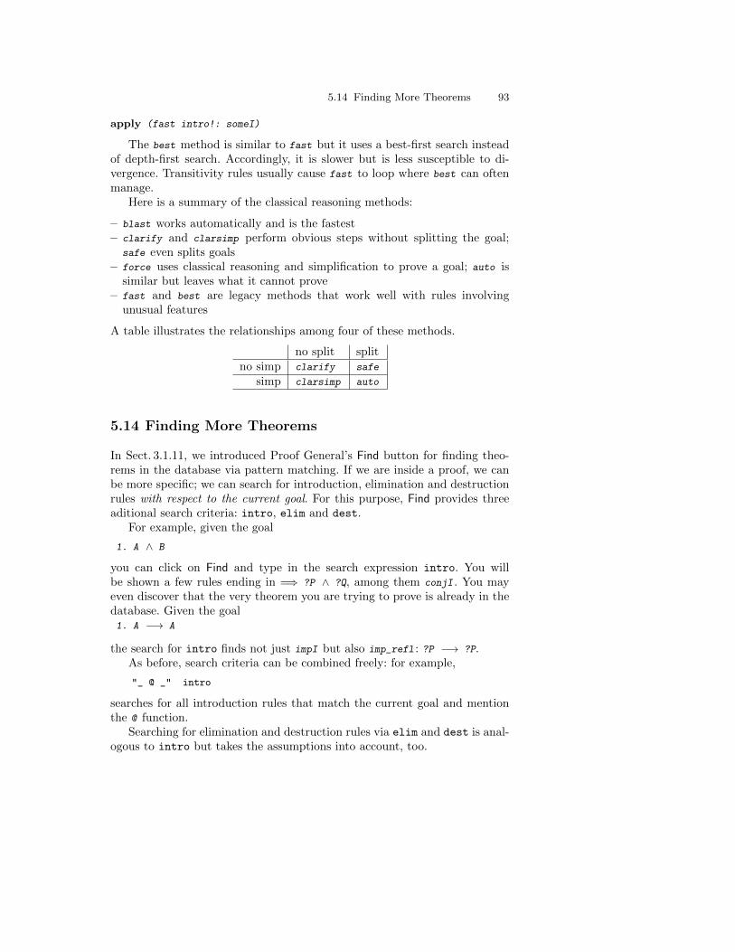
5.14 Finding More Theorems 93
apply (fast intro!: someI)
The best method is similar to fast but it uses a best-first search insteadof depth-first search. Accordingly, it is slower but is less susceptible to di-vergence. Transitivity rules usually cause fast to loop where best can oftenmanage.
Here is a summary of the classical reasoning methods:
– blast works automatically and is the fastest– clarify and clarsimp perform obvious steps without splitting the goal;
safe even splits goals– force uses classical reasoning and simplification to prove a goal; auto is
similar but leaves what it cannot prove– fast and best are legacy methods that work well with rules involving
unusual features
A table illustrates the relationships among four of these methods.
no split splitno simp clarify safe
simp clarsimp auto
5.14 Finding More Theorems
In Sect. 3.1.11, we introduced Proof General’s Find button for finding theo-rems in the database via pattern matching. If we are inside a proof, we canbe more specific; we can search for introduction, elimination and destructionrules with respect to the current goal. For this purpose, Find provides threeaditional search criteria: intro, elim and dest.
For example, given the goal
1. A ∧ B
you can click on Find and type in the search expression intro. You willbe shown a few rules ending in =⇒ ?P ∧ ?Q, among them conjI . You mayeven discover that the very theorem you are trying to prove is already in thedatabase. Given the goal1. A −→ A
the search for intro finds not just impI but also imp_refl : ?P −→ ?P.As before, search criteria can be combined freely: for example,
"_ @ _" intro
searches for all introduction rules that match the current goal and mentionthe @ function.
Searching for elimination and destruction rules via elim and dest is anal-ogous to intro but takes the assumptions into account, too.
94 5. The Rules of the Game
5.15 Forward Proof: Transforming Theorems
Forward proof means deriving new facts from old ones. It is the most funda-mental type of proof. Backward proof, by working from goals to subgoals, canhelp us find a difficult proof. But it is not always the best way of presentingthe proof thus found. Forward proof is particularly good for reasoning fromthe general to the specific. For example, consider this distributive law for thegreatest common divisor:
k × gcd(m,n) = gcd(k ×m, k × n)
Putting m = 1 we get (since gcd(1,n) = 1 and k × 1 = k)
k = gcd(k , k × n)
We have derived a new fact; if re-oriented, it might be useful for simplification.After re-orienting it and putting n = 1, we derive another useful law:
gcd(k , k) = k
Substituting values for variables — instantiation — is a forward step. Re-orientation works by applying the symmetry of equality to an equation, so ittoo is a forward step.
5.15.1 Modifying a Theorem using of, where and THEN
Let us reproduce our examples in Isabelle. Recall that in Sect. 3.5.3 we de-clared the recursive function gcd :
fun gcd :: "nat ⇒ nat ⇒ nat" where"gcd m n = (if n=0 then m else gcd n (m mod n))"
From this definition, it is possible to prove the distributive law. That takesus to the starting point for our example.
?k * gcd ?m ?n = gcd (?k * ?m) (?k * ?n) (gcd_mult_distrib2)
The first step in our derivation is to replace ?m by 1. We instantiate thetheorem using of , which identifies variables in order of their appearance fromleft to right. In this case, the variables are ?k, ?m and ?n. So, the expression[of k 1] replaces ?k by k and ?m by 1.
lemmas gcd_mult_0 = gcd_mult_distrib2 [of k 1]
The keyword lemmas declares a new theorem, which can be derived from anexisting one using attributes such as [of k 1]. The command thm gcd_mult_0
displays the result:
k * gcd 1 ?n = gcd (k * 1) (k * ?n)
5.15 Forward Proof: Transforming Theorems 95
Something is odd: k is an ordinary variable, while ?n is schematic. We didnot specify an instantiation for ?n. In its present form, the theorem does notallow substitution for k. One solution is to avoid giving an instantiation for?k : instead of a term we can put an underscore (_). For example,
gcd_mult_distrib2 [of _ 1]
replaces ?m by 1 but leaves ?k unchanged.An equivalent solution is to use the attribute where.
gcd mult distrib2 [where m=1]
While of refers to variables by their position, where refers to variables byname. Multiple instantiations are separated by and, as in this example:
gcd mult distrib2 [where m=1 and k=1]
We now continue the present example with the version of gcd_mult_0
shown above, which has k instead of ?k. Once we have replaced ?m by 1, wemust next simplify the theorem gcd_mult_0, performing the steps gcd(1,n) =1 and k × 1 = k . The simplified attribute takes a theorem and returns theresult of simplifying it, with respect to the default simplification rules:
lemmas gcd_mult_1 = gcd_mult_0 [simplified]
Again, we display the resulting theorem:
k = gcd k (k * ?n)
To re-orient the equation requires the symmetry rule:
?s = ?t =⇒ ?t = ?s (sym)
The following declaration gives our equation to sym :
lemmas gcd_mult = gcd_mult_1 [THEN sym]
Here is the result:
gcd k (k * ?n) = k
THEN sym gives the current theorem to the rule sym and returns the result-ing conclusion. The effect is to exchange the two operands of the equality.Typically THEN is used with destruction rules. Also useful is THEN spec, whichremoves the quantifier from a theorem of the form ∀x .P , and THEN mp, which
converts the implication P → Q into the rulePQ
. Similar to mp are the follow-
ing two rules, which extract the two directions of reasoning about a booleanequivalence:
[[?Q = ?P; ?Q ]] =⇒ ?P (iffD1)[[?P = ?Q; ?Q ]] =⇒ ?P (iffD2)
Normally we would never name the intermediate theorems such as gcd_mult_0and gcd_mult_1 but would combine the three forward steps:
lemmas gcd_mult = gcd_mult_distrib2 [of k 1, simplified, THEN sym]
96 5. The Rules of the Game
The directives, or attributes, are processed from left to right. This declarationof gcd_mult is equivalent to the previous one.
Such declarations can make the proof script hard to read. Better is tostate the new lemma explicitly and to prove it using a single rule methodwhose operand is expressed using forward reasoning:
lemma gcd mult [simp]: "gcd k (k*n) = k"by (rule gcd_mult_distrib2 [of k 1, simplified, THEN sym])
Compared with the previous proof of gcd_mult, this version shows the readerwhat has been proved. Also, the result will be processed in the normal way.In particular, Isabelle generalizes over all variables: the resulting theorem willhave ?k instead of k .
At the start of this section, we also saw a proof of gcd(k , k) = k . Here isthe Isabelle version:
lemma gcd self [simp]: "gcd k k = k"by (rule gcd_mult [of k 1, simplified])
!! To give of a nonatomic term, enclose it in quotation marks, as in [of "k*m"].The term must not contain unknowns: an attribute such as [of "?k*m"] will
be rejected.
5.15.2 Modifying a Theorem using OF
Recall that of generates an instance of a rule by specifying values for itsvariables. Analogous is OF, which generates an instance of a rule by specifyingfacts for its premises.
We again need the divides relation of number theory, which as we recallis defined by
?m dvd ?n ≡ ∃ k. ?n = ?m * k (dvd_def)
Suppose, for example, that we have proved the following rule. It states thatif k and n are relatively prime and if k divides m × n then k divides m.
[[gcd ?k ?n = 1; ?k dvd ?m * ?n ]] =⇒ ?k dvd ?m (relprime_dvd_mult)
We can use OF to create an instance of this rule. First, we prove an instanceof its first premise:
lemma relprime 20 81: "gcd 20 81 = 1"by (simp add: gcd.simps)
We have evaluated an application of the gcd function by simplification. Ex-pression evaluation involving recursive functions is not guaranteed to termi-nate, and it can be slow; Isabelle performs arithmetic by rewriting symbolicbit strings. Here, however, the simplification takes less than one second. Wecan give this new lemma to OF. The expression
relprime_dvd_mult [OF relprime_20_81]
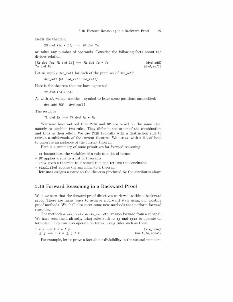
5.16 Forward Reasoning in a Backward Proof 97
yields the theorem
20 dvd (?m * 81) =⇒ 20 dvd ?m
OF takes any number of operands. Consider the following facts about thedivides relation:
[[?k dvd ?m; ?k dvd ?n ]] =⇒ ?k dvd ?m + ?n (dvd_add)?m dvd ?m (dvd_refl)
Let us supply dvd_refl for each of the premises of dvd_add :
dvd_add [OF dvd_refl dvd_refl]
Here is the theorem that we have expressed:
?k dvd (?k + ?k)
As with of, we can use the _ symbol to leave some positions unspecified:
dvd_add [OF _ dvd_refl]
The result is
?k dvd ?m =⇒ ?k dvd ?m + ?k
You may have noticed that THEN and OF are based on the same idea,namely to combine two rules. They differ in the order of the combinationand thus in their effect. We use THEN typically with a destruction rule toextract a subformula of the current theorem. We use OF with a list of factsto generate an instance of the current theorem.
Here is a summary of some primitives for forward reasoning:
– of instantiates the variables of a rule to a list of terms– OF applies a rule to a list of theorems– THEN gives a theorem to a named rule and returns the conclusion– simplified applies the simplifier to a theorem– lemmas assigns a name to the theorem produced by the attributes above
5.16 Forward Reasoning in a Backward Proof
We have seen that the forward proof directives work well within a backwardproof. There are many ways to achieve a forward style using our existingproof methods. We shall also meet some new methods that perform forwardreasoning.
The methods drule, frule, drule_tac, etc., reason forward from a subgoal.We have seen them already, using rules such as mp and spec to operate onformulae. They can also operate on terms, using rules such as these:
x = y =⇒ f x = f y (arg_cong)i ≤ j =⇒ i * k ≤ j * k (mult_le_mono1)
For example, let us prove a fact about divisibility in the natural numbers:
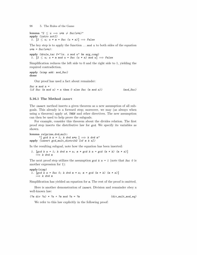
98 5. The Rules of the Game
lemma "2 ≤ u =⇒ u*m 6= Suc(u*n)"apply (intro notI)1. [[2 ≤ u; u * m = Suc (u * n) ]] =⇒ False
The key step is to apply the function . . . mod u to both sides of the equationu*m = Suc(u*n) :
apply (drule_tac f="λx. x mod u" in arg_cong)1. [[2 ≤ u; u * m mod u = Suc (u * n) mod u ]] =⇒ False
Simplification reduces the left side to 0 and the right side to 1, yielding therequired contradiction.
apply (simp add: mod_Suc)done
Our proof has used a fact about remainder:
Suc m mod n =(if Suc (m mod n) = n then 0 else Suc (m mod n)) (mod_Suc)
5.16.1 The Method insert
The insert method inserts a given theorem as a new assumption of all sub-goals. This already is a forward step; moreover, we may (as always whenusing a theorem) apply of, THEN and other directives. The new assumptioncan then be used to help prove the subgoals.
For example, consider this theorem about the divides relation. The firstproof step inserts the distributive law for gcd. We specify its variables asshown.
lemma relprime dvd mult:" [[ gcd k n = 1; k dvd m*n ]] =⇒ k dvd m"
apply (insert gcd_mult_distrib2 [of m k n])
In the resulting subgoal, note how the equation has been inserted:
1. [[gcd k n = 1; k dvd m * n; m * gcd k n = gcd (m * k) (m * n) ]]=⇒ k dvd m
The next proof step utilizes the assumption gcd k n = 1 (note that Suc 0 isanother expression for 1):
apply(simp)1. [[gcd k n = Suc 0; k dvd m * n; m = gcd (m * k) (m * n) ]]
=⇒ k dvd m
Simplification has yielded an equation for m. The rest of the proof is omitted.
Here is another demonstration of insert. Division and remainder obey awell-known law:
(?m div ?n) * ?n + ?m mod ?n = ?m (div_mult_mod_eq)
We refer to this law explicitly in the following proof:
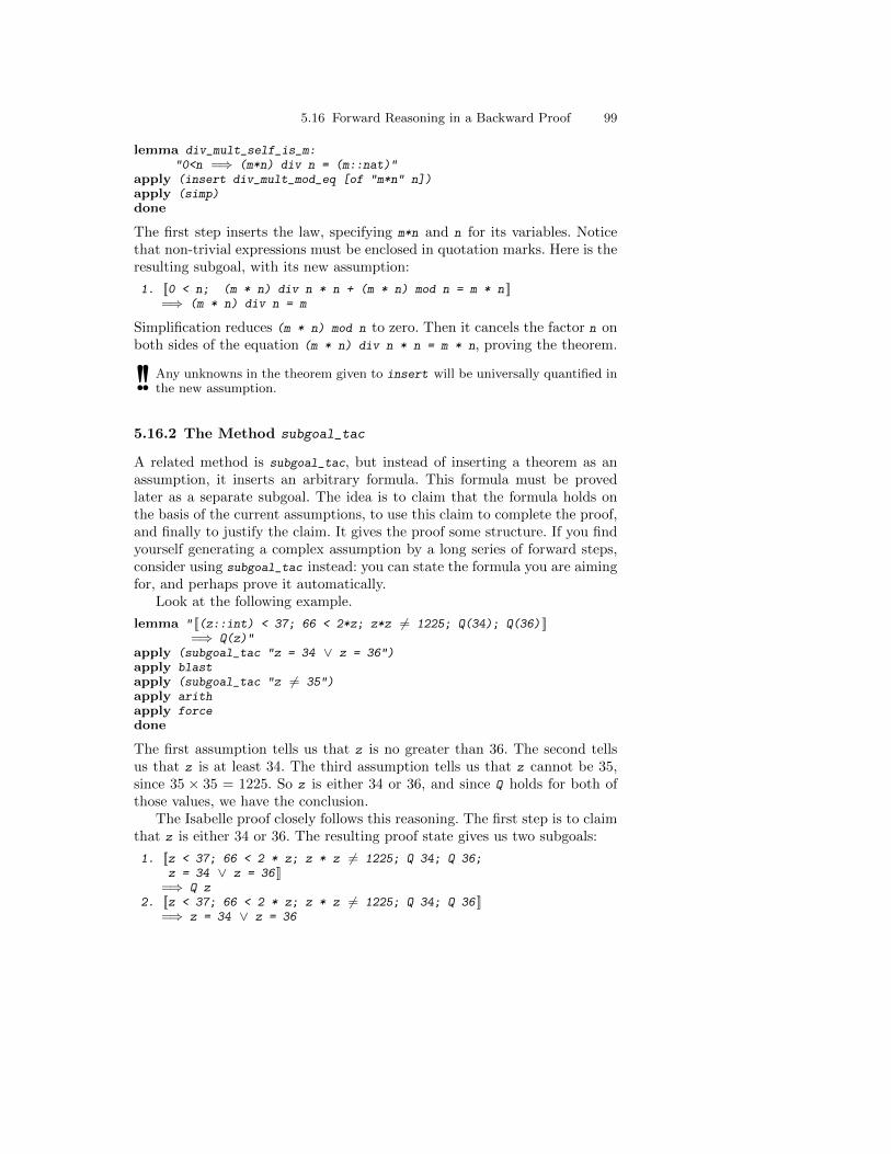
5.16 Forward Reasoning in a Backward Proof 99
lemma div_mult_self_is_m:"0<n =⇒ (m*n) div n = (m::nat)"
apply (insert div_mult_mod_eq [of "m*n" n])apply (simp)done
The first step inserts the law, specifying m*n and n for its variables. Noticethat non-trivial expressions must be enclosed in quotation marks. Here is theresulting subgoal, with its new assumption:
1. [[0 < n; (m * n) div n * n + (m * n) mod n = m * n ]]=⇒ (m * n) div n = m
Simplification reduces (m * n) mod n to zero. Then it cancels the factor n onboth sides of the equation (m * n) div n * n = m * n, proving the theorem.
!! Any unknowns in the theorem given to insert will be universally quantified inthe new assumption.
5.16.2 The Method subgoal_tac
A related method is subgoal_tac, but instead of inserting a theorem as anassumption, it inserts an arbitrary formula. This formula must be provedlater as a separate subgoal. The idea is to claim that the formula holds onthe basis of the current assumptions, to use this claim to complete the proof,and finally to justify the claim. It gives the proof some structure. If you findyourself generating a complex assumption by a long series of forward steps,consider using subgoal_tac instead: you can state the formula you are aimingfor, and perhaps prove it automatically.
Look at the following example.
lemma " [[(z::int) < 37; 66 < 2*z; z*z 6= 1225; Q(34); Q(36) ]]=⇒ Q(z)"
apply (subgoal_tac "z = 34 ∨ z = 36")apply blastapply (subgoal_tac "z 6= 35")apply arithapply forcedone
The first assumption tells us that z is no greater than 36. The second tellsus that z is at least 34. The third assumption tells us that z cannot be 35,since 35 × 35 = 1225. So z is either 34 or 36, and since Q holds for both ofthose values, we have the conclusion.
The Isabelle proof closely follows this reasoning. The first step is to claimthat z is either 34 or 36. The resulting proof state gives us two subgoals:
1. [[z < 37; 66 < 2 * z; z * z 6= 1225; Q 34; Q 36;z = 34 ∨ z = 36 ]]
=⇒ Q z2. [[z < 37; 66 < 2 * z; z * z 6= 1225; Q 34; Q 36 ]]
=⇒ z = 34 ∨ z = 36
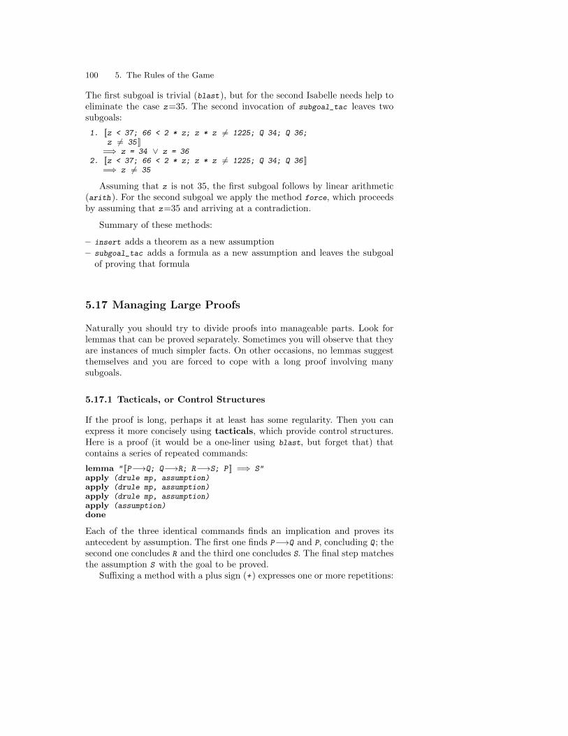
100 5. The Rules of the Game
The first subgoal is trivial (blast), but for the second Isabelle needs help toeliminate the case z=35. The second invocation of subgoal_tac leaves twosubgoals:
1. [[z < 37; 66 < 2 * z; z * z 6= 1225; Q 34; Q 36;z 6= 35 ]]
=⇒ z = 34 ∨ z = 362. [[z < 37; 66 < 2 * z; z * z 6= 1225; Q 34; Q 36 ]]
=⇒ z 6= 35
Assuming that z is not 35, the first subgoal follows by linear arithmetic(arith). For the second subgoal we apply the method force, which proceedsby assuming that z=35 and arriving at a contradiction.
Summary of these methods:
– insert adds a theorem as a new assumption– subgoal_tac adds a formula as a new assumption and leaves the subgoal
of proving that formula
5.17 Managing Large Proofs
Naturally you should try to divide proofs into manageable parts. Look forlemmas that can be proved separately. Sometimes you will observe that theyare instances of much simpler facts. On other occasions, no lemmas suggestthemselves and you are forced to cope with a long proof involving manysubgoals.
5.17.1 Tacticals, or Control Structures
If the proof is long, perhaps it at least has some regularity. Then you canexpress it more concisely using tacticals, which provide control structures.Here is a proof (it would be a one-liner using blast, but forget that) thatcontains a series of repeated commands:
lemma " [[P−→Q; Q−→R; R−→S; P ]] =⇒ S"apply (drule mp, assumption)apply (drule mp, assumption)apply (drule mp, assumption)apply (assumption)done
Each of the three identical commands finds an implication and proves itsantecedent by assumption. The first one finds P−→Q and P, concluding Q ; thesecond one concludes R and the third one concludes S. The final step matchesthe assumption S with the goal to be proved.
Suffixing a method with a plus sign (+) expresses one or more repetitions:
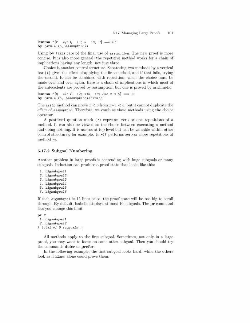
5.17 Managing Large Proofs 101
lemma " [[P−→Q; Q−→R; R−→S; P ]] =⇒ S"by (drule mp, assumption)+
Using by takes care of the final use of assumption. The new proof is moreconcise. It is also more general: the repetitive method works for a chain ofimplications having any length, not just three.
Choice is another control structure. Separating two methods by a verticalbar (|) gives the effect of applying the first method, and if that fails, tryingthe second. It can be combined with repetition, when the choice must bemade over and over again. Here is a chain of implications in which most ofthe antecedents are proved by assumption, but one is proved by arithmetic:
lemma " [[Q−→R; P−→Q; x<5−→P; Suc x < 5 ]] =⇒ R"by (drule mp, (assumption|arith))+
The arith method can prove x < 5 from x +1 < 5, but it cannot duplicate theeffect of assumption. Therefore, we combine these methods using the choiceoperator.
A postfixed question mark (?) expresses zero or one repetitions of amethod. It can also be viewed as the choice between executing a methodand doing nothing. It is useless at top level but can be valuable within othercontrol structures; for example, (m+)? performs zero or more repetitions ofmethod m.
5.17.2 Subgoal Numbering
Another problem in large proofs is contending with huge subgoals or manysubgoals. Induction can produce a proof state that looks like this:
1. bigsubgoal12. bigsubgoal23. bigsubgoal34. bigsubgoal45. bigsubgoal56. bigsubgoal6
If each bigsubgoal is 15 lines or so, the proof state will be too big to scrollthrough. By default, Isabelle displays at most 10 subgoals. The pr commandlets you change this limit:
pr 21. bigsubgoal12. bigsubgoal2
A total of 6 subgoals...
All methods apply to the first subgoal. Sometimes, not only in a largeproof, you may want to focus on some other subgoal. Then you should trythe commands defer or prefer.
In the following example, the first subgoal looks hard, while the otherslook as if blast alone could prove them:
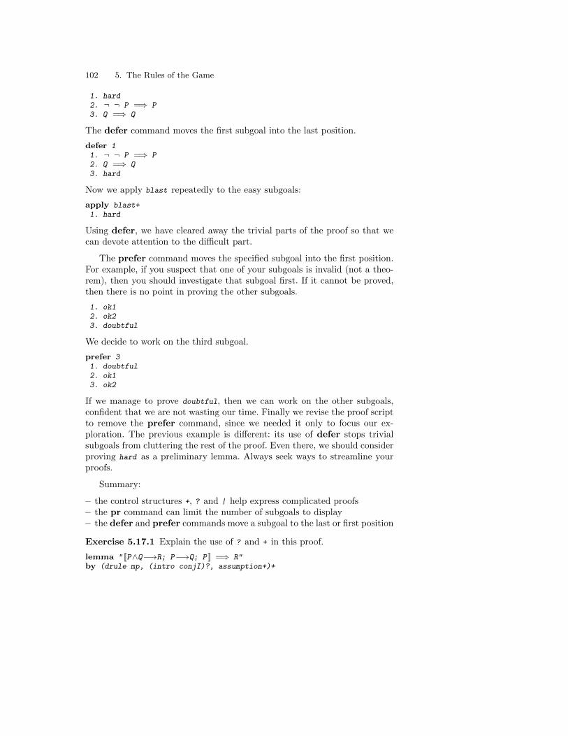
102 5. The Rules of the Game
1. hard2. ¬ ¬ P =⇒ P3. Q =⇒ Q
The defer command moves the first subgoal into the last position.
defer 11. ¬ ¬ P =⇒ P2. Q =⇒ Q3. hard
Now we apply blast repeatedly to the easy subgoals:
apply blast+1. hard
Using defer, we have cleared away the trivial parts of the proof so that wecan devote attention to the difficult part.
The prefer command moves the specified subgoal into the first position.For example, if you suspect that one of your subgoals is invalid (not a theo-rem), then you should investigate that subgoal first. If it cannot be proved,then there is no point in proving the other subgoals.
1. ok12. ok23. doubtful
We decide to work on the third subgoal.
prefer 31. doubtful2. ok13. ok2
If we manage to prove doubtful, then we can work on the other subgoals,confident that we are not wasting our time. Finally we revise the proof scriptto remove the prefer command, since we needed it only to focus our ex-ploration. The previous example is different: its use of defer stops trivialsubgoals from cluttering the rest of the proof. Even there, we should considerproving hard as a preliminary lemma. Always seek ways to streamline yourproofs.
Summary:
– the control structures +, ? and | help express complicated proofs– the pr command can limit the number of subgoals to display– the defer and prefer commands move a subgoal to the last or first position
Exercise 5.17.1 Explain the use of ? and + in this proof.
lemma " [[P∧Q−→R; P−→Q; P ]] =⇒ R"by (drule mp, (intro conjI)?, assumption+)+
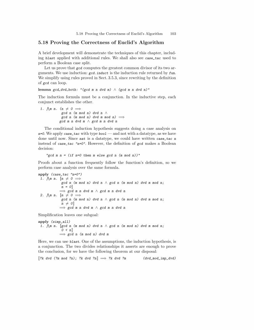
5.18 Proving the Correctness of Euclid’s Algorithm 103
5.18 Proving the Correctness of Euclid’s Algorithm
A brief development will demonstrate the techniques of this chapter, includ-ing blast applied with additional rules. We shall also see case_tac used toperform a Boolean case split.
Let us prove that gcd computes the greatest common divisor of its two ar-guments. We use induction: gcd.induct is the induction rule returned by fun.We simplify using rules proved in Sect. 3.5.3, since rewriting by the definitionof gcd can loop.
lemma gcd dvd both: "(gcd m n dvd m) ∧ (gcd m n dvd n)"
The induction formula must be a conjunction. In the inductive step, eachconjunct establishes the other.
1.∧m n. (n 6= 0 =⇒
gcd n (m mod n) dvd n ∧gcd n (m mod n) dvd m mod n) =⇒
gcd m n dvd m ∧ gcd m n dvd n
The conditional induction hypothesis suggests doing a case analysis onn=0. We apply case_tac with type bool — and not with a datatype, as we havedone until now. Since nat is a datatype, we could have written case_tac n
instead of case_tac "n=0". However, the definition of gcd makes a Booleandecision:
"gcd m n = (if n=0 then m else gcd n (m mod n))"
Proofs about a function frequently follow the function’s definition, so weperform case analysis over the same formula.
apply (case_tac "n=0")1.
∧m n. [[n 6= 0 =⇒
gcd n (m mod n) dvd n ∧ gcd n (m mod n) dvd m mod n;n = 0 ]]
=⇒ gcd m n dvd m ∧ gcd m n dvd n2.
∧m n. [[n 6= 0 =⇒
gcd n (m mod n) dvd n ∧ gcd n (m mod n) dvd m mod n;n 6= 0 ]]
=⇒ gcd m n dvd m ∧ gcd m n dvd n
Simplification leaves one subgoal:
apply (simp_all)1.
∧m n. [[gcd n (m mod n) dvd n ∧ gcd n (m mod n) dvd m mod n;
0 < n ]]=⇒ gcd n (m mod n) dvd m
Here, we can use blast. One of the assumptions, the induction hypothesis, isa conjunction. The two divides relationships it asserts are enough to provethe conclusion, for we have the following theorem at our disposal:
[[?k dvd (?m mod ?n); ?k dvd ?n ]] =⇒ ?k dvd ?m (dvd_mod_imp_dvd)
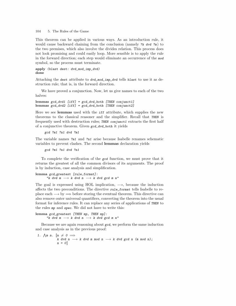
104 5. The Rules of the Game
This theorem can be applied in various ways. As an introduction rule, itwould cause backward chaining from the conclusion (namely ?k dvd ?m) tothe two premises, which also involve the divides relation. This process doesnot look promising and could easily loop. More sensible is to apply the rulein the forward direction; each step would eliminate an occurrence of the mod
symbol, so the process must terminate.
apply (blast dest: dvd_mod_imp_dvd)done
Attaching the dest attribute to dvd_mod_imp_dvd tells blast to use it as de-struction rule; that is, in the forward direction.
We have proved a conjunction. Now, let us give names to each of the twohalves:
lemmas gcd_dvd1 [iff] = gcd_dvd_both [THEN conjunct1]lemmas gcd_dvd2 [iff] = gcd_dvd_both [THEN conjunct2]
Here we see lemmas used with the iff attribute, which supplies the newtheorems to the classical reasoner and the simplifier. Recall that THEN isfrequently used with destruction rules; THEN conjunct1 extracts the first halfof a conjunctive theorem. Given gcd_dvd_both it yields
gcd ?m1 ?n1 dvd ?m1
The variable names ?m1 and ?n1 arise because Isabelle renames schematicvariables to prevent clashes. The second lemmas declaration yields
gcd ?m1 ?n1 dvd ?n1
To complete the verification of the gcd function, we must prove that itreturns the greatest of all the common divisors of its arguments. The proofis by induction, case analysis and simplification.
lemma gcd greatest [rule format]:"k dvd m −→ k dvd n −→ k dvd gcd m n"
The goal is expressed using HOL implication, −→, because the inductionaffects the two preconditions. The directive rule_format tells Isabelle to re-place each −→ by =⇒ before storing the eventual theorem. This directive canalso remove outer universal quantifiers, converting the theorem into the usualformat for inference rules. It can replace any series of applications of THEN tothe rules mp and spec. We did not have to write this:
lemma gcd_greatest [THEN mp, THEN mp]:"k dvd m −→ k dvd n −→ k dvd gcd m n"
Because we are again reasoning about gcd, we perform the same inductionand case analysis as in the previous proof:
1.∧m n. [[n 6= 0 =⇒
k dvd n −→ k dvd m mod n −→ k dvd gcd n (m mod n);n = 0 ]]
5.18 Proving the Correctness of Euclid’s Algorithm 105
=⇒ k dvd m −→ k dvd n −→ k dvd gcd m n2.
∧m n. [[n 6= 0 =⇒
k dvd n −→ k dvd m mod n −→ k dvd gcd n (m mod n);n 6= 0 ]]
=⇒ k dvd m −→ k dvd n −→ k dvd gcd m n
Simplification proves both subgoals.
apply (simp_all add: dvd_mod)done
In the first, where n=0, the implication becomes trivial: k dvd gcd m n goesto k dvd m. The second subgoal is proved by an unfolding of gcd, using thisrule about divides:
[[?f dvd ?m; ?f dvd ?n ]] =⇒ ?f dvd ?m mod ?n (dvd_mod)
The facts proved above can be summarized as a single logical equivalence.This step gives us a chance to see another application of blast.
theorem gcd greatest iff [iff]:"(k dvd gcd m n) = (k dvd m ∧ k dvd n)"
by (blast intro!: gcd_greatest intro: dvd_trans)
This theorem concisely expresses the correctness of the gcd function. We stateit with the iff attribute so that Isabelle can use it to remove some occur-rences of gcd. The theorem has a one-line proof using blast supplied withtwo additional introduction rules. The exclamation mark (intro!) signifiessafe rules, which are applied aggressively. Rules given without the exclama-tion mark are applied reluctantly and their uses can be undone if the searchbacktracks. Here the unsafe rule expresses transitivity of the divides relation:
[[?m dvd ?n; ?n dvd ?p ]] =⇒ ?m dvd ?p (dvd_trans)
Applying dvd_trans as an introduction rule entails a risk of looping, for itmultiplies occurrences of the divides symbol. However, this proof relies ontransitivity reasoning. The rule gcd greatest is safe to apply aggressivelybecause it yields simpler subgoals. The proof implicitly uses gcd_dvd1 andgcd_dvd2 as safe rules, because they were declared using iff.

6. Sets, Functions and Relations
This chapter describes the formalization of typed set theory, which is thebasis of much else in HOL. For example, an inductive definition yields a set,and the abstract theories of relations regard a relation as a set of pairs. Thechapter introduces the well-known constants such as union and intersection,as well as the main operations on relations, such as converse, compositionand transitive closure. Functions are also covered. They are not sets in HOL,but many of their properties concern sets: the range of a function is a set,and the inverse image of a function maps sets to sets.
This chapter will be useful to anybody who plans to develop a substantialproof. Sets are convenient for formalizing computer science concepts suchas grammars, logical calculi and state transition systems. Isabelle can provemany statements involving sets automatically.
This chapter ends with a case study concerning model checking for thetemporal logic CTL. Most of the other examples are simple. The chapterpresents a small selection of built-in theorems in order to point out some keyproperties of the various constants and to introduce you to the notation.
Natural deduction rules are provided for the set theory constants, butthey are seldom used directly, so only a few are presented here.
6.1 Sets
HOL’s set theory should not be confused with traditional, untyped set theory,in which everything is a set. Our sets are typed. In a given set, all elementshave the same type, say τ , and the set itself has type τ set .
We begin with intersection, union and complement. In addition tothe membership relation, there is a symbol for its negation. These pointscan be seen below.
Here are the natural deduction rules for intersection. Note the resemblanceto those for conjunction.
[[c ∈ A; c ∈ B ]] =⇒ c ∈ A ∩ B (IntI)c ∈ A ∩ B =⇒ c ∈ A (IntD1)c ∈ A ∩ B =⇒ c ∈ B (IntD2)
Here are two of the many installed theorems concerning set complement.Note that it is denoted by a minus sign.
108 6. Sets, Functions and Relations
(c ∈ - A) = (c /∈ A) (Compl_iff)- (A ∪ B) = - A ∩ - B (Compl_Un)
Set difference is the intersection of a set with the complement of anotherset. Here we also see the syntax for the empty set and for the universal set.
A ∩ (B - A) = {} (Diff_disjoint)A ∪ - A = UNIV (Compl_partition)
The subset relation holds between two sets just if every element of oneis also an element of the other. This relation is reflexive. These are its naturaldeduction rules:
(∧x. x ∈ A =⇒ x ∈ B) =⇒ A ⊆ B (subsetI)
[[A ⊆ B; c ∈ A ]] =⇒ c ∈ B (subsetD)
In harder proofs, you may need to apply subsetD giving a specific term for c.However, blast can instantly prove facts such as this one:
(A ∪ B ⊆ C) = (A ⊆ C ∧ B ⊆ C) (Un_subset_iff)
Here is another example, also proved automatically:
lemma "(A ⊆ -B) = (B ⊆ -A)"by blast
This is the same example using ascii syntax, illustrating a pitfall:
lemma "(A <= -B) = (B <= -A)"
The proof fails. It is not a statement about sets, due to overloading; therelation symbol <= can be any relation, not just subset. In this general form,the statement is not valid. Putting in a type constraint forces the variablesto denote sets, allowing the proof to succeed:
lemma "((A:: ’a set) <= -B) = (B <= -A)"
Section 8.3 below describes overloading. Incidentally, A ⊆ -B asserts that thesets A and B are disjoint.
Two sets are equal if they contain the same elements. This is the principleof extensionality for sets.
(∧x. (x ∈ A) = (x ∈ B)) =⇒ A = B (set_ext)
Extensionality can be expressed as A = B ⇐⇒ (A ⊆ B) ∧ (B ⊆ A). Thefollowing rules express both directions of this equivalence. Proving a set equa-tion using equalityI allows the two inclusions to be proved independently.
[[A ⊆ B; B ⊆ A ]] =⇒ A = B (equalityI)
[[A = B; [[A ⊆ B; B ⊆ A ]] =⇒ P ]] =⇒ P (equalityE)
6.1 Sets 109
6.1.1 Finite Set Notation
Finite sets are expressed using the constant insert , which is a form of union:
insert a A = {a} ∪ A (insert_is_Un)
The finite set expression {a,b} abbreviates insert a (insert b {}). Manyfacts about finite sets can be proved automatically:
lemma "{a,b} ∪ {c,d} = {a,b,c,d}"by blast
Not everything that we would like to prove is valid. Consider this attempt:
lemma "{a,b} ∩ {b,c} = {b}"apply auto
The proof fails, leaving the subgoal b=c. To see why it fails, consider a correctversion:
lemma "{a,b} ∩ {b,c} = (if a=c then {a,b} else {b})"apply simpby blast
Our mistake was to suppose that the various items were distinct. Anotherremark: this proof uses two methods, namely simp and blast . Calling simp
eliminates the if -then -else expression, which blast cannot break down. Thecombined methods (namely force and auto) can prove this fact in one step.
6.1.2 Set Comprehension
The set comprehension {x. P} expresses the set of all elements that satisfy thepredicate P. Two laws describe the relationship between set comprehensionand the membership relation:
(a ∈ {x. P x}) = P a (mem_Collect_eq){x. x ∈ A} = A (Collect_mem_eq)
Facts such as these have trivial proofs:
lemma "{x. P x ∨ x ∈ A} = {x. P x} ∪ A"
lemma "{x. P x −→ Q x} = -{x. P x} ∪ {x. Q x}"
Isabelle has a general syntax for comprehension, which is best describedthrough an example:
lemma "{p*q | p q. p∈prime ∧ q∈prime} ={z. ∃ p q. z = p*q ∧ p∈prime ∧ q∈prime}"
The left and right hand sides of this equation are identical. The syntax usedin the left-hand side abbreviates the right-hand side: in this case, all numbersthat are the product of two primes. The syntax provides a neat way of ex-pressing any set given by an expression built up from variables under specific
110 6. Sets, Functions and Relations
constraints. The drawback is that it hides the true form of the expression,with its existential quantifiers.
Remark. We do not need sets at all. They are essentially equivalent topredicate variables, which are allowed in higher-order logic. The main benefitof sets is their notation; we can write x∈A and {z. P} where predicates wouldrequire writing A(x) and λz. P.
6.1.3 Binding Operators
Universal and existential quantifications may range over sets, with the obvi-ous meaning. Here are the natural deduction rules for the bounded universalquantifier. Occasionally you will need to apply bspec with an explicit instan-tiation of the variable x :
(∧x. x ∈ A =⇒ P x) =⇒ ∀ x∈A. P x (ballI)
[[∀ x∈A. P x; x ∈ A ]] =⇒ P x (bspec)
Dually, here are the natural deduction rules for the bounded existential quan-tifier. You may need to apply bexI with an explicit instantiation:
[[P x; x ∈ A ]] =⇒ ∃ x∈A. P x (bexI)[[∃ x∈A. P x;
∧x. [[x ∈ A; P x ]] =⇒ Q ]] =⇒ Q (bexE)
Unions can be formed over the values of a given set. The syntax is⋃x∈A. B or UN x:A. B in ascii. Indexed union satisfies this basic law:
(b ∈ (⋃x∈A. B x)) = (∃ x∈A. b ∈ B x) (UN_iff)
It has two natural deduction rules similar to those for the existential quanti-fier. Sometimes UN_I must be applied explicitly:
[[a ∈ A; b ∈ B a ]] =⇒ b ∈ (⋃x∈A. B x) (UN_I)
[[b ∈ (⋃x∈A. B x);
∧x. [[x ∈ A; b ∈ B x ]] =⇒ R ]] =⇒ R (UN_E)
The following built-in abbreviation (see Sect. 4.1.4) lets us express the unionover a type:
(⋃x. B x) ≡ (
⋃x∈UNIV. B x)
We may also express the union of a set of sets, written Union C in ascii:
(A ∈⋃C) = (∃ X∈C. A ∈ X) (Union_iff)
Intersections are treated dually, although they seem to be used less oftenthan unions. The syntax below would be INT x: A. B and Inter C in ascii.Among others, these theorems are available:
(b ∈ (⋂x∈A. B x)) = (∀ x∈A. b ∈ B x) (INT_iff)
(A ∈⋂C) = (∀ X∈C. A ∈ X) (Inter_iff)
Isabelle uses logical equivalences such as those above in automatic proof.Unions, intersections and so forth are not simply replaced by their definitions.Instead, membership tests are simplified. For example, x ∈ A∪B is replacedby x ∈ A ∨ x ∈ B .
6.2 Functions 111
The internal form of a comprehension involves the constant Collect ,which occasionally appears when a goal or theorem is displayed. For example,Collect P is the same term as {x. P x}. The same thing can happen withquantifiers: All P is ∀ x. P x and Ex P is ∃ x. P x ; also Ball A P is ∀ x∈A. P
x and Bex A P is ∃ x∈A. P x. For indexed unions and intersections, you maysee the constants UNION and INTER . The internal constant for εx .P(x ) is Eps .
We have only scratched the surface of Isabelle/HOL’s set theory, whichprovides hundreds of theorems for your use.
6.1.4 Finiteness and Cardinality
The predicate finite holds of all finite sets. Isabelle/HOL includes manyfamiliar theorems about finiteness and cardinality (card). For example, wehave theorems concerning the cardinalities of unions, intersections and thepowerset:
[[finite A; finite B ]]=⇒ card A + card B = card (A ∪ B) + card (A ∩ B) (card_Un_Int)
finite A =⇒ card (Pow A) = 2 ^ card A (card_Pow)
finite A =⇒card {B. B ⊆ A ∧ card B = k} = card A choose k (n_subsets)
Writing |A| as n, the last of these theorems says that the number of k -elementsubsets of A is
(nk
).
6.2 Functions
This section describes a few concepts that involve functions. Some of the moreimportant theorems are given along with the names. A few sample proofsappear. Unlike with set theory, however, we cannot simply state lemmas andexpect them to be proved using blast.
6.2.1 Function Basics
Two functions are equal if they yield equal results given equal arguments.This is the principle of extensionality for functions:
(∧x. f x = g x) =⇒ f = g (ext)
Function update is useful for modelling machine states. It has the obvi-ous definition and many useful facts are proved about it. In particular, thefollowing equation is installed as a simplification rule:
(f(x:=y)) z = (if z = x then y else f z) (fun_upd_apply)
112 6. Sets, Functions and Relations
Two syntactic points must be noted. In (f(x:=y)) z we are applying anupdated function to an argument; the outer parentheses are essential. A seriesof two or more updates can be abbreviated as shown on the left-hand side ofthis theorem:
f(x:=y, x:=z) = f(x:=z) (fun_upd_upd)
Note also that we can write f(x:=z) with only one pair of parentheses whenit is not being applied to an argument.
The identity function and function composition are defined:
id ≡ λx. x (id_def)f ◦ g ≡ λx. f (g x) (o_def)
Many familiar theorems concerning the identity and composition are proved.For example, we have the associativity of composition:
f ◦ (g ◦ h) = f ◦ g ◦ h (o_assoc)
6.2.2 Injections, Surjections, Bijections
A function may be injective, surjective or bijective:
inj_on f A ≡ ∀ x∈A. ∀ y∈A. f x = f y −→ x = y (inj_on_def)surj f ≡ ∀ y. ∃ x. y = f x (surj_def)bij f ≡ inj f ∧ surj f (bij_def)
The second argument of inj_on lets us express that a function is injective overa given set. This refinement is useful in higher-order logic, where functions aretotal; in some cases, a function’s natural domain is a subset of its domain type.Writing inj f abbreviates inj_on f UNIV, for when f is injective everywhere.
The operator inv expresses the inverse of a function. In general theinverse may not be well behaved. We have the usual laws, such as these:
inj f =⇒ inv f (f x) = x (inv_f_f)surj f =⇒ f (inv f y) = y (surj_f_inv_f)bij f =⇒ inv (inv f) = f (inv_inv_eq)
Theorems involving these concepts can be hard to prove. The followingexample is easy, but it cannot be proved automatically. To begin with, weneed a law that relates the equality of functions to equality over all arguments:
(f = g) = (∀ x. f x = g x) (fun_eq_iff)
This is just a restatement of extensionality. Our lemma states that an injec-tion can be cancelled from the left side of function composition:
lemma "inj f =⇒ (f o g = f o h) = (g = h)"apply (simp add: fun_eq_iff inj_on_def)apply autodone
The first step of the proof invokes extensionality and the definitions ofinjectiveness and composition. It leaves one subgoal:
6.3 Relations 113
1. ∀ x y. f x = f y −→ x = y =⇒(∀ x. f (g x) = f (h x)) = (∀ x. g x = h x)
This can be proved using the auto method.
6.2.3 Function Image
The image of a set under a function is a most useful notion. It has theobvious definition:
f ‘ A ≡ {y. ∃ x∈A. y = f x} (image_def)
Here are some of the many facts proved about image:
(f ◦ g) ‘ r = f ‘ g ‘ r (image_compose)f‘(A ∪ B) = f‘A ∪ f‘B (image_Un)inj f =⇒ f‘(A ∩ B) = f‘A ∩ f‘B (image_Int)
Laws involving image can often be proved automatically. Here are twoexamples, illustrating connections with indexed union and with the generalsyntax for comprehension:
lemma "f‘A ∪ g‘A = (⋃x∈A. {f x, g x})"
lemma "f ‘ {(x,y). P x y} = {f(x,y) | x y. P x y}"
A function’s range is the set of values that the function can take on. Itis, in fact, the image of the universal set under that function. There is noconstant range. Instead, range abbreviates an application of image to UNIV :
range f f‘UNIV
Few theorems are proved specifically for range ; in most cases, you shouldlook for a more general theorem concerning images.
Inverse image is also useful. It is defined as follows:
f -‘ B ≡ {x. f x ∈ B} (vimage_def)
This is one of the facts proved about it:
f -‘ (- A) = - f -‘ A (vimage_Compl)
6.3 Relations
A relation is a set of pairs. As such, the set operations apply to them. Forinstance, we may form the union of two relations. Other primitives are definedspecifically for relations.
114 6. Sets, Functions and Relations
6.3.1 Relation Basics
The identity relation, also known as equality, has the obvious definition:
Id ≡ {p. ∃ x. p = (x,x)} (Id_def)
Composition of relations (the infix O) is also available:
r O s = {(x,z). ∃ y. (x,y) ∈ s ∧ (y,z) ∈ r} (relcomp_unfold)
This is one of the many lemmas proved about these concepts:
R O Id = R (R_O_Id)
Composition is monotonic, as are most of the primitives appearing in thischapter. We have many theorems similar to the following one:
[[r’ ⊆ r; s’ ⊆ s ]] =⇒ r’ O s’ ⊆ r O s (relcomp_mono)
The converse or inverse of a relation exchanges the roles of the twooperands. We use the postfix notation r−1 or r^-1 in ASCII.
((a,b) ∈ r−1) = ((b,a) ∈ r) (converse_iff)
Here is a typical law proved about converse and composition:
(r O s)−1 = s−1 O r−1 (converse_relcomp)
The image of a set under a relation is defined analogously to image undera function:
(b ∈ r ‘‘ A) = (∃ x∈A. (x,b) ∈ r) (Image_iff)
It satisfies many similar laws.The domain and range of a relation are defined in the standard way:
(a ∈ Domain r) = (∃ y. (a,y) ∈ r) (Domain_iff)(a ∈ Range r) = (∃ y. (y,a) ∈ r) (Range_iff)
Iterated composition of a relation is available. The notation overloads thatof exponentiation. Two simplification rules are installed:
R ^ 0 = IdR ^ Suc n = R O R^n
6.3.2 The Reflexive and Transitive Closure
The reflexive and transitive closure of the relation r is written with apostfix syntax. In ASCII we write r^* and in symbol notation r∗. It is theleast solution of the equation
r∗ = Id ∪ (r O r∗) (rtrancl_unfold)
Among its basic properties are three that serve as introduction rules:
(a, a) ∈ r∗ (rtrancl_refl)p ∈ r =⇒ p ∈ r∗ (r_into_rtrancl)[[(a,b) ∈ r∗; (b,c) ∈ r∗]] =⇒ (a,c) ∈ r∗ (rtrancl_trans)
6.3 Relations 115
Induction over the reflexive transitive closure is available:
[[(a, b) ∈ r∗; P a;∧y z. [[(a, y) ∈ r∗; (y, z) ∈ r; P y ]] =⇒ P z ]]
=⇒ P b (rtrancl_induct)
Idempotence is one of the laws proved about the reflexive transitive closure:
(r∗)∗ = r∗ (rtrancl_idemp)
The transitive closure is similar. The ASCII syntax is r^+. It has twointroduction rules:
p ∈ r =⇒ p ∈ r+ (r_into_trancl)[[(a, b) ∈ r+; (b, c) ∈ r+]] =⇒ (a, c) ∈ r+ (trancl_trans)
The induction rule resembles the one shown above. A typical lemma statesthat transitive closure commutes with the converse operator:
(r−1)+ = (r+)−1 (trancl_converse)
6.3.3 A Sample Proof
The reflexive transitive closure also commutes with the converse operator. Letus examine the proof. Each direction of the equivalence is proved separately.The two proofs are almost identical. Here is the first one:
lemma rtrancl_converseD: "(x,y) ∈ (r−1)∗ =⇒ (y,x) ∈ r∗"apply (erule rtrancl_induct)apply (rule rtrancl_refl)
apply (blast intro: rtrancl_trans)done
The first step of the proof applies induction, leaving these subgoals:
1. (x, x) ∈ r∗
2.∧y z. [[(x,y) ∈ (r−1)∗; (y,z) ∈ r−1; (y,x) ∈ r∗]]
=⇒ (z,x) ∈ r∗
The first subgoal is trivial by reflexivity. The second follows by first elimi-nating the converse operator, yielding the assumption (z,y) ∈ r, and thenapplying the introduction rules shown above. The same proof script handlesthe other direction:
lemma rtrancl_converseI: "(y,x) ∈ r∗ =⇒ (x,y) ∈ (r−1)∗"apply (erule rtrancl_induct)apply (rule rtrancl_refl)
apply (blast intro: rtrancl_trans)done
Finally, we combine the two lemmas to prove the desired equation:
lemma rtrancl_converse: "(r−1)∗ = (r∗)−1"by (auto intro: rtrancl_converseI dest: rtrancl_converseD)
116 6. Sets, Functions and Relations
!! This trivial proof requires auto rather than blast because of a subtle issueinvolving ordered pairs. Here is a subgoal that arises internally after the rules
equalityI and subsetI have been applied:
1.∧x. x ∈ (r−1)∗ =⇒ x ∈ (r∗)−1
We cannot apply rtrancl_converseD . It refers to ordered pairs, while x is a vari-able of product type. The simp and blast methods can do nothing, so let us tryclarify :
1.∧a b. (a,b) ∈ (r−1)∗ =⇒ (b,a) ∈ r∗
Now that x has been replaced by the pair (a,b), we can proceed. Other methodsthat split variables in this way are force, auto, fast and best. Section 8.1 willdiscuss proof techniques for ordered pairs in more detail.
6.4 Well-Founded Relations and Induction
A well-founded relation captures the notion of a terminating process. Com-plex recursive functions definitions must specify a well-founded relation thatjustifies their termination [18]. Most of the forms of induction found in math-ematics are merely special cases of induction over a well-founded relation.
Intuitively, the relation ≺ is well-founded if it admits no infinite de-scending chains
· · · ≺ a2 ≺ a1 ≺ a0.
Well-foundedness can be hard to show. The various formulations are all com-plicated. However, often a relation is well-founded by construction. HOL pro-vides theorems concerning ways of constructing a well-founded relation. Themost familiar way is to specify a measure function f into the natural num-bers, when x ≺ y ⇐⇒ f x < f y; we write this particular relation asmeasure f.
!! You may want to skip the rest of this section until you need to perform acomplex recursive function definition or induction. The induction rule returned
by fun is good enough for most purposes. We use an explicit well-founded inductiononly in Sect. 9.2.4.
Isabelle/HOL declares less_than as a relation object, that is, a set ofpairs of natural numbers. Two theorems tell us that this relation behaves asexpected and that it is well-founded:
((x,y) ∈ less_than) = (x < y) (less_than_iff)wf less_than (wf_less_than)
The notion of measure generalizes to the inverse image of a relation.Given a relation r and a function f, we express a new relation using f as ameasure. An infinite descending chain on this new relation would give riseto an infinite descending chain on r. Isabelle/HOL defines this concept andproves a theorem stating that it preserves well-foundedness:
6.5 Fixed Point Operators 117
inv_image r f ≡ {(x,y). (f x, f y) ∈ r} (inv_image_def)wf r =⇒ wf (inv_image r f) (wf_inv_image)
A measure function involves the natural numbers. The relation measure
size justifies primitive recursion and structural induction over a datatype.Isabelle/HOL defines measure as shown:
measure ≡ inv_image less_than (measure_def)wf (measure f) (wf_measure)
Of the other constructions, the most important is the lexicographicproduct of two relations. It expresses the standard dictionary ordering overpairs. We write ra <*lex*> rb, where ra and rb are the two operands. Thelexicographic product satisfies the usual definition and it preserves well-foundedness:
ra <*lex*> rb ≡{((a,b),(a’,b’)). (a,a’) ∈ ra ∨
a=a’ ∧ (b,b’) ∈ rb} (lex_prod_def)
[[wf ra; wf rb ]] =⇒ wf (ra <*lex*> rb) (wf_lex_prod)
The multiset ordering, useful for hard termination proofs, is availablein the Library [4]. Baader and Nipkow [3, Sect. 2.5] discuss it.
Induction comes in many forms, including traditional mathematical in-duction, structural induction on lists and induction on size. All are instancesof the following rule, for a suitable well-founded relation ≺:
[∀y . y ≺ x → P(y)]....
P(x )
P(a)
To show P(a) for a particular term a, it suffices to show P(x ) for arbi-trary x under the assumption that P(y) holds for y ≺ x . Intuitively, thewell-foundedness of ≺ ensures that the chains of reasoning are finite.
In Isabelle, the induction rule is expressed like this:
[[wf r;∧x. ∀ y. (y,x) ∈ r −→ P y =⇒ P x ]] =⇒ P a (wf_induct)
Here wf r expresses that the relation r is well-founded.Many familiar induction principles are instances of this rule. For example,
the predecessor relation on the natural numbers is well-founded; inductionover it is mathematical induction. The “tail of” relation on lists is well-founded; induction over it is structural induction.
6.5 Fixed Point Operators
Fixed point operators define sets recursively. They are invoked implicitlywhen making an inductive definition, as discussed in Chap. 7 below. However,
118 6. Sets, Functions and Relations
they can be used directly, too. The least or strongest fixed point yields aninductive definition; the greatest or weakest fixed point yields a coinductivedefinition. Mathematicians may wish to note that the existence of these fixedpoints is guaranteed by the Knaster-Tarski theorem.
!! Casual readers should skip the rest of this section. We use fixed point operatorsonly in Sect. 6.6.
The theory applies only to monotonic functions. Isabelle’s definition ofmonotone is overloaded over all orderings:
mono f ≡ ∀ A B. A ≤ B −→ f A ≤ f B (mono_def)
For fixed point operators, the ordering will be the subset relation: if A ⊆ Bthen we expect f (A) ⊆ f (B). In addition to its definition, monotonicity hasthe obvious introduction and destruction rules:
(∧A B. A ≤ B =⇒ f A ≤ f B) =⇒ mono f (monoI)
[[mono f; A ≤ B ]] =⇒ f A ≤ f B (monoD)
The most important properties of the least fixed point are that it is afixed point and that it enjoys an induction rule:
mono f =⇒ lfp f = f (lfp f) (lfp_unfold)
[[a ∈ lfp f; mono f;∧x. x ∈ f (lfp f ∩ {x. P x}) =⇒ P x ]] =⇒ P a (lfp_induct)
The induction rule shown above is more convenient than the basic one derivedfrom the minimality of lfp . Observe that both theorems demand mono f asa premise.
The greatest fixed point is similar, but it has a coinduction rule:
mono f =⇒ gfp f = f (gfp f) (gfp_unfold)[[mono f; a ∈ X; X ⊆ f (X ∪ gfp f) ]] =⇒ a ∈ gfp f (coinduct)
A bisimulation is perhaps the best-known concept defined as a greatestfixed point. Exhibiting a bisimulation to prove the equality of two agents ina process algebra is an example of coinduction. The coinduction rule can bestrengthened in various ways.
6.6 Case Study: Verified Model Checking
This chapter ends with a case study concerning model checking for Com-putation Tree Logic (CTL), a temporal logic. Model checking is a populartechnique for the verification of finite state systems (implementations) withrespect to temporal logic formulae (specifications) [8, 16]. Its foundations areset theoretic and this section will explore them in HOL. This is done in twosteps. First we consider a simple modal logic called propositional dynamiclogic (PDL). We then proceed to the temporal logic CTL, which is used in
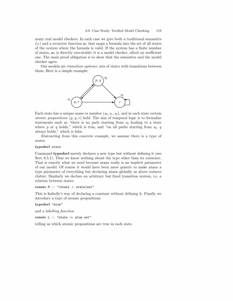
6.6 Case Study: Verified Model Checking 119
many real model checkers. In each case we give both a traditional semantics(|=) and a recursive function mc that maps a formula into the set of all statesof the system where the formula is valid. If the system has a finite numberof states, mc is directly executable: it is a model checker, albeit an inefficientone. The main proof obligation is to show that the semantics and the modelchecker agree.
Our models are transition systems: sets of states with transitions betweenthem. Here is a simple example:
����
p, qs0
��
������� @
@@@R
����
q , rs1 -��
��r�
s2
Each state has a unique name or number (s0, s1, s2), and in each state certainatomic propositions (p, q , r) hold. The aim of temporal logic is to formalizestatements such as “there is no path starting from s2 leading to a statewhere p or q holds,” which is true, and “on all paths starting from s0, qalways holds,” which is false.
Abstracting from this concrete example, we assume there is a type ofstates:
typedecl state
Command typedecl merely declares a new type but without defining it (seeSect. 8.5.1). Thus we know nothing about the type other than its existence.That is exactly what we need because state really is an implicit parameterof our model. Of course it would have been more generic to make state atype parameter of everything but declaring state globally as above reducesclutter. Similarly we declare an arbitrary but fixed transition system, i.e. arelation between states:
consts M :: "(state × state)set"
This is Isabelle’s way of declaring a constant without defining it. Finally weintroduce a type of atomic propositions
typedecl "atom"
and a labelling function
consts L :: "state ⇒ atom set"
telling us which atomic propositions are true in each state.
120 6. Sets, Functions and Relations
6.6.1 Propositional Dynamic Logic — PDL
The formulae of PDL are built up from atomic propositions via negation andconjunction and the two temporal connectives AX and EF . Since formulae areessentially syntax trees, they are naturally modelled as a datatype:1
datatype formula = Atom "atom"| Neg formula| And formula formula| AX formula| EF formula
This resembles the boolean expression case study in Sect. 2.5.6. A validityrelation between states and formulae specifies the semantics. The syntax an-notation allows us to write s |= f instead of valid s f . The definition is byrecursion over the syntax:
primrec valid :: "state ⇒ formula ⇒ bool" ("(_ |= _)" [80,80] 80)where"s |= Atom a = (a ∈ L s)" |"s |= Neg f = (¬(s |= f))" |"s |= And f g = (s |= f ∧ s |= g)" |"s |= AX f = (∀ t. (s,t) ∈ M −→ t |= f)" |"s |= EF f = (∃ t. (s,t) ∈ M∗ ∧ t |= f)"
The first three equations should be self-explanatory. The temporal formulaAX f means that f is true in All neX t states whereas EF f means that thereExists some Future state in which f is true. The future is expressed via ∗,the reflexive transitive closure. Because of reflexivity, the future includes thepresent.
Now we come to the model checker itself. It maps a formula into the setof states where the formula is true. It too is defined by recursion over thesyntax:
primrec mc :: "formula ⇒ state set" where"mc(Atom a) = {s. a ∈ L s}" |"mc(Neg f) = -mc f" |"mc(And f g) = mc f ∩ mc g" |"mc(AX f) = {s. ∀ t. (s,t) ∈ M −→ t ∈ mc f}" |"mc(EF f) = lfp(λT. mc f ∪ (M−1 ‘‘ T))"
Only the equation for EF deserves some comments. Remember that the postfix−1 and the infix ‘‘ are predefined and denote the converse of a relation andthe image of a set under a relation. Thus M−1 ‘‘ T is the set of all predecessorsof T and the least fixed point (lfp) of λT. mc f ∪ M−1 ‘‘ T is the least setT containing mc f and all predecessors of T. If you find it hard to see thatmc (EF f) contains exactly those states from which there is a path to a statewhere f is true, do not worry — this will be proved in a moment.
1 The customary definition of PDL [13] looks quite different from ours, but thetwo are easily shown to be equivalent.
6.6 Case Study: Verified Model Checking 121
First we prove monotonicity of the function inside lfp in order to makesure it really has a least fixed point.
lemma mono_ef: "mono(λT. A ∪ (M−1 ‘‘ T))"apply(rule monoI)apply blastdone
Now we can relate model checking and semantics. For the EF case we need aseparate lemma:
lemma EF_lemma:"lfp(λT. A ∪ (M−1 ‘‘ T)) = {s. ∃ t. (s,t) ∈ M∗ ∧ t ∈ A}"
The equality is proved in the canonical fashion by proving that each setincludes the other; the inclusion is shown pointwise:
apply(rule equalityI)apply(rule subsetI)apply(simp)
Simplification leaves us with the following first subgoal
1.∧s. s ∈ lfp (λT. A ∪ M−1 ‘‘ T) =⇒ ∃ t. (s, t) ∈ M∗ ∧ t ∈ A
A total of 2 subgoals...
which is proved by lfp -induction:
apply(erule lfp_induct_set)apply(rule mono_ef)
apply(simp)
Having disposed of the monotonicity subgoal, simplification leaves us withthe following goal:
1.∧x. x ∈ A ∨
x ∈ M−1 ‘‘ (lfp (...) ∩ {x. ∃ t. (x, t) ∈ M∗ ∧ t ∈ A})=⇒ ∃ t. (x, t) ∈ M∗ ∧ t ∈ A
It is proved by blast, using the transitivity of M∗.
apply(blast intro: rtrancl_trans)
We now return to the second set inclusion subgoal, which is again provedpointwise:
apply(rule subsetI)apply(simp, clarify)
After simplification and clarification we are left with
1.∧x t. [[(x, t) ∈ M∗; t ∈ A ]] =⇒ x ∈ lfp (λT. A ∪ M−1 ‘‘ T)
This goal is proved by induction on (s, t) ∈ M∗. But since the modelchecker works backwards (from t to s), we cannot use the induction theoremrtrancl_induct : it works in the forward direction. Fortunately the converseinduction theorem converse_rtrancl_induct already exists:
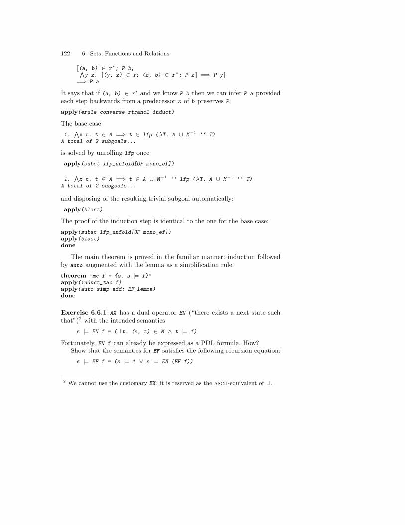
122 6. Sets, Functions and Relations
[[(a, b) ∈ r∗; P b;∧y z. [[(y, z) ∈ r; (z, b) ∈ r∗; P z ]] =⇒ P y ]]
=⇒ P a
It says that if (a, b) ∈ r∗ and we know P b then we can infer P a providedeach step backwards from a predecessor z of b preserves P.
apply(erule converse_rtrancl_induct)
The base case
1.∧x t. t ∈ A =⇒ t ∈ lfp (λT. A ∪ M−1 ‘‘ T)
A total of 2 subgoals...
is solved by unrolling lfp once
apply(subst lfp_unfold[OF mono_ef])
1.∧x t. t ∈ A =⇒ t ∈ A ∪ M−1 ‘‘ lfp (λT. A ∪ M−1 ‘‘ T)
A total of 2 subgoals...
and disposing of the resulting trivial subgoal automatically:
apply(blast)
The proof of the induction step is identical to the one for the base case:
apply(subst lfp_unfold[OF mono_ef])apply(blast)done
The main theorem is proved in the familiar manner: induction followedby auto augmented with the lemma as a simplification rule.
theorem "mc f = {s. s |= f}"apply(induct_tac f)apply(auto simp add: EF_lemma)done
Exercise 6.6.1 AX has a dual operator EN (“there exists a next state suchthat”)2 with the intended semantics
s |= EN f = (∃ t. (s, t) ∈ M ∧ t |= f)
Fortunately, EN f can already be expressed as a PDL formula. How?Show that the semantics for EF satisfies the following recursion equation:
s |= EF f = (s |= f ∨ s |= EN (EF f))
2 We cannot use the customary EX : it is reserved as the ascii-equivalent of ∃ .
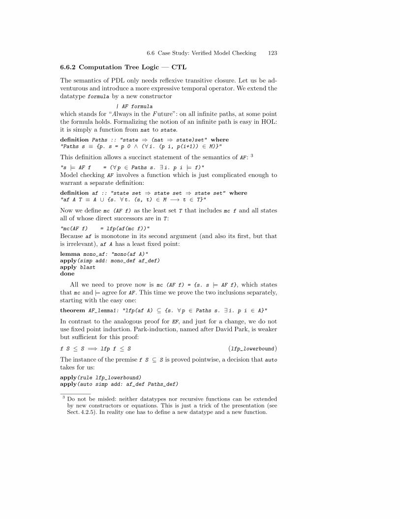
6.6 Case Study: Verified Model Checking 123
6.6.2 Computation Tree Logic — CTL
The semantics of PDL only needs reflexive transitive closure. Let us be ad-venturous and introduce a more expressive temporal operator. We extend thedatatype formula by a new constructor
| AF formula
which stands for “Always in the Future”: on all infinite paths, at some pointthe formula holds. Formalizing the notion of an infinite path is easy in HOL:it is simply a function from nat to state.
definition Paths :: "state ⇒ (nat ⇒ state)set" where"Paths s ≡ {p. s = p 0 ∧ (∀ i. (p i, p(i+1)) ∈ M)}"
This definition allows a succinct statement of the semantics of AF : 3
"s |= AF f = (∀ p ∈ Paths s. ∃ i. p i |= f)"
Model checking AF involves a function which is just complicated enough towarrant a separate definition:
definition af :: "state set ⇒ state set ⇒ state set" where"af A T ≡ A ∪ {s. ∀ t. (s, t) ∈ M −→ t ∈ T}"
Now we define mc (AF f) as the least set T that includes mc f and all statesall of whose direct successors are in T :
"mc(AF f) = lfp(af(mc f))"
Because af is monotone in its second argument (and also its first, but thatis irrelevant), af A has a least fixed point:
lemma mono_af: "mono(af A)"apply(simp add: mono_def af_def)apply blastdone
All we need to prove now is mc (AF f) = {s. s |= AF f}, which statesthat mc and |= agree for AF . This time we prove the two inclusions separately,starting with the easy one:
theorem AF_lemma1: "lfp(af A) ⊆ {s. ∀ p ∈ Paths s. ∃ i. p i ∈ A}"
In contrast to the analogous proof for EF, and just for a change, we do notuse fixed point induction. Park-induction, named after David Park, is weakerbut sufficient for this proof:
f S ≤ S =⇒ lfp f ≤ S (lfp_lowerbound)
The instance of the premise f S ⊆ S is proved pointwise, a decision that autotakes for us:
apply(rule lfp_lowerbound)apply(auto simp add: af_def Paths_def)
3 Do not be misled: neither datatypes nor recursive functions can be extendedby new constructors or equations. This is just a trick of the presentation (seeSect. 4.2.5). In reality one has to define a new datatype and a new function.
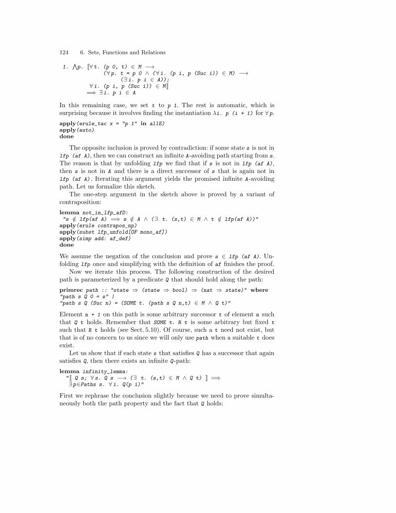
124 6. Sets, Functions and Relations
1.∧p. [[∀ t. (p 0, t) ∈ M −→
(∀ p. t = p 0 ∧ (∀ i. (p i, p (Suc i)) ∈ M) −→(∃ i. p i ∈ A));
∀ i. (p i, p (Suc i)) ∈ M ]]=⇒ ∃ i. p i ∈ A
In this remaining case, we set t to p 1. The rest is automatic, which issurprising because it involves finding the instantiation λi. p (i + 1) for ∀ p.
apply(erule_tac x = "p 1" in allE)apply(auto)done
The opposite inclusion is proved by contradiction: if some state s is not inlfp (af A), then we can construct an infinite A -avoiding path starting from s.The reason is that by unfolding lfp we find that if s is not in lfp (af A),then s is not in A and there is a direct successor of s that is again not inlfp (af A) . Iterating this argument yields the promised infinite A -avoidingpath. Let us formalize this sketch.
The one-step argument in the sketch above is proved by a variant ofcontraposition:
lemma not_in_lfp_afD:"s /∈ lfp(af A) =⇒ s /∈ A ∧ (∃ t. (s,t) ∈ M ∧ t /∈ lfp(af A))"
apply(erule contrapos_np)apply(subst lfp_unfold[OF mono_af])apply(simp add: af_def)done
We assume the negation of the conclusion and prove s ∈ lfp (af A). Un-folding lfp once and simplifying with the definition of af finishes the proof.
Now we iterate this process. The following construction of the desiredpath is parameterized by a predicate Q that should hold along the path:
primrec path :: "state ⇒ (state ⇒ bool) ⇒ (nat ⇒ state)" where"path s Q 0 = s" |"path s Q (Suc n) = (SOME t. (path s Q n,t) ∈ M ∧ Q t)"
Element n + 1 on this path is some arbitrary successor t of element n suchthat Q t holds. Remember that SOME t. R t is some arbitrary but fixed t
such that R t holds (see Sect. 5.10). Of course, such a t need not exist, butthat is of no concern to us since we will only use path when a suitable t doesexist.
Let us show that if each state s that satisfies Q has a successor that againsatisfies Q, then there exists an infinite Q -path:
lemma infinity_lemma:" [[ Q s; ∀ s. Q s −→ (∃ t. (s,t) ∈ M ∧ Q t) ]] =⇒∃ p∈Paths s. ∀ i. Q(p i)"
First we rephrase the conclusion slightly because we need to prove simulta-neously both the path property and the fact that Q holds:
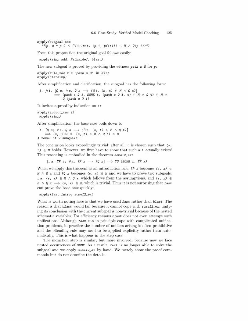
6.6 Case Study: Verified Model Checking 125
apply(subgoal_tac"∃ p. s = p 0 ∧ (∀ i::nat. (p i, p(i+1)) ∈ M ∧ Q(p i))")
From this proposition the original goal follows easily:
apply(simp add: Paths_def, blast)
The new subgoal is proved by providing the witness path s Q for p :
apply(rule_tac x = "path s Q" in exI)apply(clarsimp)
After simplification and clarification, the subgoal has the following form:
1.∧i. [[Q s; ∀ s. Q s −→ (∃ t. (s, t) ∈ M ∧ Q t) ]]
=⇒ (path s Q i, SOME t. (path s Q i, t) ∈ M ∧ Q t) ∈ M ∧Q (path s Q i)
It invites a proof by induction on i :
apply(induct_tac i)apply(simp)
After simplification, the base case boils down to
1. [[Q s; ∀ s. Q s −→ (∃ t. (s, t) ∈ M ∧ Q t) ]]=⇒ (s, SOME t. (s, t) ∈ M ∧ Q t) ∈ M
A total of 2 subgoals...
The conclusion looks exceedingly trivial: after all, t is chosen such that (s,
t) ∈ M holds. However, we first have to show that such a t actually exists!This reasoning is embodied in the theorem someI2_ex :
[[∃ a. ?P a;∧x. ?P x =⇒ ?Q x ]] =⇒ ?Q (SOME x. ?P x)
When we apply this theorem as an introduction rule, ?P x becomes (s, x) ∈M ∧ Q x and ?Q x becomes (s, x) ∈ M and we have to prove two subgoals:∃ a. (s, a) ∈ M ∧ Q a, which follows from the assumptions, and (s, x) ∈M ∧ Q x =⇒ (s, x) ∈ M, which is trivial. Thus it is not surprising that fast
can prove the base case quickly:
apply(fast intro: someI2_ex)
What is worth noting here is that we have used fast rather than blast. Thereason is that blast would fail because it cannot cope with someI2_ex : unify-ing its conclusion with the current subgoal is non-trivial because of the nestedschematic variables. For efficiency reasons blast does not even attempt suchunifications. Although fast can in principle cope with complicated unifica-tion problems, in practice the number of unifiers arising is often prohibitiveand the offending rule may need to be applied explicitly rather than auto-matically. This is what happens in the step case.
The induction step is similar, but more involved, because now we facenested occurrences of SOME. As a result, fast is no longer able to solve thesubgoal and we apply someI2_ex by hand. We merely show the proof com-mands but do not describe the details:
126 6. Sets, Functions and Relations
apply(simp)apply(rule someI2_ex)apply(blast)
apply(rule someI2_ex)apply(blast)
apply(blast)done
Function path has fulfilled its purpose now and can be forgotten. It wasmerely defined to provide the witness in the proof of the infinity_lemma.Aficionados of minimal proofs might like to know that we could have giventhe witness without having to define a new function: the term
rec_nat s (λn t. SOME u. (t, u) ∈ M ∧ Q u)
is extensionally equal to path s Q, where rec_nat is the predefined primitiverecursor on nat.
At last we can prove the opposite direction of AF_lemma1 :
theorem AF_lemma2: "{s. ∀ p ∈ Paths s. ∃ i. p i ∈ A} ⊆ lfp(af A)"
The proof is again pointwise and then by contraposition:
apply(rule subsetI)apply(erule contrapos_pp)apply simp
1.∧x. x /∈ lfp (af A) =⇒ ∃ p∈Paths x. ∀ i. p i /∈ A
Applying the infinity_lemma as a destruction rule leaves two subgoals, thesecond premise of infinity_lemma and the original subgoal:
apply(drule infinity_lemma)
1.∧x. ∀ s. s /∈ lfp (af A) −→ (∃ t. (s, t) ∈ M ∧ t /∈ lfp (af A))
2.∧x. ∃ p∈Paths x. ∀ i. p i /∈ lfp (af A) =⇒∃ p∈Paths x. ∀ i. p i /∈ A
Both are solved automatically:
apply(auto dest: not_in_lfp_afD)done
If you find these proofs too complicated, we recommend that you readSect. 9.2.4, where we show how inductive definitions lead to simpler argu-ments.
The main theorem is proved as for PDL, except that we also derive thenecessary equality lfp(af A) = ... by combining AF_lemma1 and AF_lemma2
on the spot:
theorem "mc f = {s. s |= f}"apply(induct_tac f)apply(auto simp add: EF_lemma equalityI[OF AF_lemma1 AF_lemma2])done
6.6 Case Study: Verified Model Checking 127
The language defined above is not quite CTL. The latter also includes anuntil-operator EU f g with semantics “there Exists a path where f is trueU ntil g becomes true”. We need an auxiliary function:
primrecuntil:: "state set ⇒ state set ⇒ state ⇒ state list ⇒ bool" where"until A B s [] = (s ∈ B)" |"until A B s (t#p) = (s ∈ A ∧ (s,t) ∈ M ∧ until A B t p)"
Expressing the semantics of EU is now straightforward:
s |= EU f g = (∃ p. until {t. t |= f} {t. t |= g} s p)
Note that EU is not definable in terms of the other operators!Model checking EU is again a least fixed point construction:
mc(EU f g) = lfp(λT. mc g ∪ mc f ∩ (M−1 ‘‘ T))
Exercise 6.6.2 Extend the datatype of formulae by the above until operatorand prove the equivalence between semantics and model checking, i.e. that
mc (EU f g) = {s. s |= EU f g}
For more CTL exercises see, for example, Huth and Ryan [16].
Let us close this section with a few words about the executability of ourmodel checkers. It is clear that if all sets are finite, they can be represented aslists and the usual set operations are easily implemented. Only lfp requiresa little thought. Fortunately, theory While_Combinator in the Library [4] pro-vides a theorem stating that in the case of finite sets and a monotone func-tion F, the value of lfp F can be computed by iterated application of F to {}
until a fixed point is reached. It is actually possible to generate executablefunctional programs from HOL definitions, but that is beyond the scope ofthe tutorial.

7. Inductively Defined Sets
This chapter is dedicated to the most important definition principle afterrecursive functions and datatypes: inductively defined sets.
We start with a simple example: the set of even numbers. A slightlymore complicated example, the reflexive transitive closure, is the subjectof Sect. 7.2. In particular, some standard induction heuristics are discussed.Advanced forms of inductive definitions are discussed in Sect. 7.3. To demon-strate the versatility of inductive definitions, the chapter closes with a casestudy from the realm of context-free grammars. The first two sections arerequired reading for anybody interested in mathematical modelling.
!! Predicates can also be defined inductively. See Sect. 7.1.7.
7.1 The Set of Even Numbers
The set of even numbers can be inductively defined as the least set containing0 and closed under the operation +2. Obviously, even can also be expressedusing the divides relation (dvd). We shall prove below that the two formula-tions coincide. On the way we shall examine the primary means of reasoningabout inductively defined sets: rule induction.
7.1.1 Making an Inductive Definition
Using inductive set, we declare the constant even to be a set of naturalnumbers with the desired properties.
inductive set even :: "nat set" wherezero[intro!]: "0 ∈ even" |step[intro!]: "n ∈ even =⇒ (Suc (Suc n)) ∈ even"
An inductive definition consists of introduction rules. The first one abovestates that 0 is even; the second states that if n is even, then so is n + 2.Given this declaration, Isabelle generates a fixed point definition for Even.evenand proves theorems about it, thus following the definitional approach (seeSect. 2.8). These theorems include the introduction rules specified in the dec-laration, an elimination rule for case analysis and an induction rule. We can
130 7. Inductively Defined Sets
refer to these theorems by automatically-generated names. Here are two ex-amples:
0 ∈ Even.even (even.zero)
n ∈ Even.even =⇒ Suc (Suc n) ∈ Even.even (even.step)
The introduction rules can be given attributes. Here both rules are spec-ified as intro!, directing the classical reasoner to apply them aggressively.Obviously, regarding 0 as even is safe. The step rule is also safe becausen + 2 is even if and only if n is even. We prove this equivalence later.
7.1.2 Using Introduction Rules
Our first lemma states that numbers of the form 2× k are even. Introductionrules are used to show that specific values belong to the inductive set. Suchproofs typically involve induction, perhaps over some other inductive set.
lemma two_times_even[intro!]: "2*k ∈ even"apply (induct_tac k)apply auto
done
The first step is induction on the natural number k, which leaves two subgoals:
1. 2 * 0 ∈ Even.even2.
∧n. 2 * n ∈ Even.even =⇒ 2 * Suc n ∈ Even.even
Here auto simplifies both subgoals so that they match the introduction rules,which are then applied automatically.
Our ultimate goal is to prove the equivalence between the traditionaldefinition of even (using the divides relation) and our inductive definition.One direction of this equivalence is immediate by the lemma just proved,whose intro! attribute ensures it is applied automatically.
lemma dvd_imp_even: "2 dvd n =⇒ n ∈ even"by (auto simp add: dvd_def)
7.1.3 Rule Induction
From the definition of the set Even.even, Isabelle has generated an inductionrule:
[[x ∈ Even.even; P 0;∧n. [[n ∈ Even.even; P n ]]
=⇒ P (Suc (Suc n)) ]]=⇒ P x (even.induct)
A property P holds for every even number provided it holds for 0 and is closedunder the operation Suc(Suc ·). Then P is closed under the introduction rulesfor Even.even, which is the least set closed under those rules. This type ofinductive argument is called rule induction.
7.1 The Set of Even Numbers 131
Apart from the double application of Suc, the induction rule above resem-bles the familiar mathematical induction, which indeed is an instance of ruleinduction; the natural numbers can be defined inductively to be the least setcontaining 0 and closed under Suc.
Induction is the usual way of proving a property of the elements of aninductively defined set. Let us prove that all members of the set Even.even
are multiples of two.
lemma even_imp_dvd: "n ∈ even =⇒ 2 dvd n"
We begin by applying induction. Note that even.induct has the form ofan elimination rule, so we use the method erule. We get two subgoals:
apply (erule even.induct)
1. semiring_parity_class.even 02.
∧n. [[n ∈ Even.even; semiring_parity_class.even n ]]
=⇒ semiring_parity_class.even (Suc (Suc n))
We unfold the definition of dvd in both subgoals, proving the first one andsimplifying the second:
apply (simp_all add: dvd_def)
1.∧n. [[n ∈ Even.even; ∃ k. n = 2 * k ]] =⇒ ∃ k. Suc (Suc n) = 2 * k
The next command eliminates the existential quantifier from the assumptionand replaces n by 2 * k.
apply clarify
1.∧n k. 2 * k ∈ Even.even =⇒ ∃ ka. Suc (Suc (2 * k)) = 2 * ka
To conclude, we tell Isabelle that the desired value is Suc k. With this hint,the subgoal falls to simp.
apply (rule_tac x = "Suc k" in exI, simp)
Combining the previous two results yields our objective, the equivalencerelating Even.even and dvd.
theorem even_iff_dvd: "(n ∈ even) = (2 dvd n)"by (blast intro: dvd_imp_even even_imp_dvd)
7.1.4 Generalization and Rule Induction
Before applying induction, we typically must generalize the induction for-mula. With rule induction, the required generalization can be hard to findand sometimes requires a complete reformulation of the problem. In this ex-ample, our first attempt uses the obvious statement of the result. It fails:
lemma "Suc (Suc n) ∈ even =⇒ n ∈ even"
132 7. Inductively Defined Sets
apply (erule even.induct)oops
Rule induction finds no occurrences of Suc (Suc n) in the conclusion,which it therefore leaves unchanged. (Look at even.induct to see why thishappens.) We have these subgoals:
1. n ∈ Even.even2.
∧na. [[na ∈ Even.even; n ∈ Even.even ]] =⇒ n ∈ Even.even
The first one is hopeless. Rule induction on a non-variable term discardsinformation, and usually fails. How to deal with such situations in general isdescribed in Sect. 9.2.1 below. In the current case the solution is easy becausewe have the necessary inverse, subtraction:
lemma even_imp_even_minus_2: "n ∈ even =⇒ n - 2 ∈ even"apply (erule even.induct)apply auto
done
This lemma is trivially inductive. Here are the subgoals:
1. 0 - 2 ∈ Even.even2.
∧n. [[n ∈ Even.even; n - 2 ∈ Even.even ]] =⇒ Suc (Suc n) - 2 ∈ Even.even
The first is trivial because 0 - 2 simplifies to 0, which is even. The second istrivial too: Suc (Suc n) - 2 simplifies to n, matching the assumption.
Using our lemma, we can easily prove the result we originally wanted:
lemma Suc_Suc_even_imp_even: "Suc (Suc n) ∈ even =⇒ n ∈ even"by (drule even_imp_even_minus_2, simp)
We have just proved the converse of the introduction rule even.step. Thissuggests proving the following equivalence. We give it the iff attribute be-cause of its obvious value for simplification.
lemma [iff]: "((Suc (Suc n)) ∈ even) = (n ∈ even)"by (blast dest: Suc_Suc_even_imp_even)
7.1.5 Rule Inversion
Case analysis on an inductive definition is called rule inversion. It is fre-quently used in proofs about operational semantics. It can be highly effectivewhen it is applied automatically. Let us look at how rule inversion is done inIsabelle/HOL.
Recall that Even.even is the minimal set closed under these two rules:
0 ∈ Even.evenn ∈ Even.even =⇒ Suc (Suc n) ∈ Even.even
Minimality means that Even.even contains only the elements that these rulesforce it to contain. If we are told that a belongs to Even.even then there areonly two possibilities. Either a is 0 or else a has the form Suc (Suc n), forsome suitable n that belongs to Even.even. That is the gist of the cases rule,which Isabelle proves for us when it accepts an inductive definition:
7.1 The Set of Even Numbers 133
[[a ∈ Even.even; a = 0 =⇒ P;∧n. [[a = Suc (Suc n); n ∈ Even.even ]]
=⇒ P ]]=⇒ P (even.cases)
This general rule is less useful than instances of it for specific patterns. Forexample, if a has the form Suc (Suc n) then the first case becomes irrele-vant, while the second case tells us that n belongs to Even.even. Isabelle willgenerate this instance for us:
inductive cases Suc_Suc_cases [elim!]: "Suc(Suc n) ∈ even"
The inductive cases command generates an instance of the cases rulefor the supplied pattern and gives it the supplied name:
[[Suc (Suc n) ∈ Even.even; n ∈ Even.even =⇒ P ]] =⇒ P (Suc_Suc_cases)
Applying this as an elimination rule yields one case where even.cases wouldyield two. Rule inversion works well when the conclusions of the introduc-tion rules involve datatype constructors like Suc and # (list “cons”); freenessreasoning discards all but one or two cases.
In the inductive cases command we supplied an attribute, elim!, in-dicating that this elimination rule can be applied aggressively. The originalcases rule would loop if used in that manner because the pattern a matcheseverything.
The rule Suc_Suc_cases is equivalent to the following implication:
Suc (Suc n) ∈ Even.even =⇒ n ∈ Even.even
Just above we devoted some effort to reaching precisely this result. Yet wecould have obtained it by a one-line declaration, dispensing with the lemmaeven_imp_even_minus_2. This example also justifies the terminology rule in-version: the new rule inverts the introduction rule even.step. In general, arule can be inverted when the set of elements it introduces is disjoint fromthose of the other introduction rules.
For one-off applications of rule inversion, use the ind_cases method. Hereis an example:
apply (ind_cases "Suc(Suc n) ∈ even")
The specified instance of the cases rule is generated, then applied as anelimination rule.
To summarize, every inductive definition produces a cases rule. The in-ductive cases command stores an instance of the cases rule for a givenpattern. Within a proof, the ind_cases method applies an instance of thecases rule.
The even numbers example has shown how inductive definitions can beused. Later examples will show that they are actually worth using.
134 7. Inductively Defined Sets
7.1.6 Mutually Inductive Definitions
Just as there are datatypes defined by mutual recursion, there are sets definedby mutual induction. As a trivial example we consider the even and oddnatural numbers:
inductive setEven :: "nat set" andOdd :: "nat set"
wherezero: "0 ∈ Even"
| EvenI: "n ∈ Odd =⇒ Suc n ∈ Even"| OddI: "n ∈ Even =⇒ Suc n ∈ Odd"
The mutually inductive definition of multiple sets is no different from thatof a single set, except for induction: just as for mutually recursive datatypes,induction needs to involve all the simultaneously defined sets. In the abovecase, the induction rule is called Even_Odd.induct (simply concatenate thenames of the sets involved) and has the conclusion
(?x ∈ Even −→ ?P ?x) ∧ (?y ∈ Odd −→ ?Q ?y)
If we want to prove that all even numbers are divisible by two, we haveto generalize the statement as follows:
lemma "(m ∈ Even −→ 2 dvd m) ∧ (n ∈ Odd −→ 2 dvd (Suc n))"
The proof is by rule induction. Because of the form of the induction theorem,it is applied by rule rather than erule as for ordinary inductive definitions:
apply(rule Even_Odd.induct)
1. even 02.
∧n. [[n ∈ Odd; even (Suc n) ]] =⇒ even (Suc n)
3.∧n. [[n ∈ Even; even n ]] =⇒ even (Suc (Suc n))
The first two subgoals are proved by simplification and the final one canbe proved in the same manner as in Sect. 7.1.3 where the same subgoal wasencountered before. We do not show the proof script.
7.1.7 Inductively Defined Predicates
Instead of a set of even numbers one can also define a predicate on nat :
inductive evn :: "nat ⇒ bool" wherezero: "evn 0" |step: "evn n =⇒ evn(Suc(Suc n))"
Everything works as before, except that you write inductive instead of in-ductive set and evn n instead of n ∈ Even. When defining an n-ary rela-tion as a predicate, it is recommended to curry the predicate: its type should
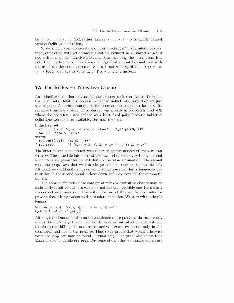
7.2 The Reflexive Transitive Closure 135
be τ1 ⇒ . . . ⇒ τn ⇒ bool rather than τ1 × . . . × τn ⇒ bool. The curriedversion facilitates inductions.
When should you choose sets and when predicates? If you intend to com-bine your notion with set theoretic notation, define it as an inductive set. Ifnot, define it as an inductive predicate, thus avoiding the ∈ notation. Butnote that predicates of more than one argument cannot be combined withthe usual set theoretic operators: P ∪ Q is not well-typed if P, Q :: τ1 ⇒τ2 ⇒ bool, you have to write λx y. P x y ∧ Q x y instead.
7.2 The Reflexive Transitive Closure
An inductive definition may accept parameters, so it can express functionsthat yield sets. Relations too can be defined inductively, since they are justsets of pairs. A perfect example is the function that maps a relation to itsreflexive transitive closure. This concept was already introduced in Sect. 6.3,where the operator ∗ was defined as a least fixed point because inductivedefinitions were not yet available. But now they are:
inductive setrtc :: "(’a × ’a)set ⇒ (’a × ’a)set" ("_*" [1000] 999)for r :: "(’a × ’a)set"
wherertc_refl[iff]: "(x,x) ∈ r*"
| rtc_step: " [[ (x,y) ∈ r; (y,z) ∈ r* ]] =⇒ (x,z) ∈ r*"
The function rtc is annotated with concrete syntax: instead of rtc r we canwrite r*. The actual definition consists of two rules. Reflexivity is obvious andis immediately given the iff attribute to increase automation. The secondrule, rtc_step, says that we can always add one more r -step to the left.Although we could make rtc_step an introduction rule, this is dangerous: therecursion in the second premise slows down and may even kill the automatictactics.
The above definition of the concept of reflexive transitive closure may besufficiently intuitive but it is certainly not the only possible one: for a start,it does not even mention transitivity. The rest of this section is devoted toproving that it is equivalent to the standard definition. We start with a simplelemma:
lemma [intro]: "(x,y) ∈ r =⇒ (x,y) ∈ r*"by(blast intro: rtc_step)
Although the lemma itself is an unremarkable consequence of the basic rules,it has the advantage that it can be declared an introduction rule withoutthe danger of killing the automatic tactics because r* occurs only in theconclusion and not in the premise. Thus some proofs that would otherwiseneed rtc_step can now be found automatically. The proof also shows thatblast is able to handle rtc_step. But some of the other automatic tactics are
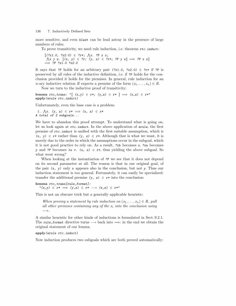
136 7. Inductively Defined Sets
more sensitive, and even blast can be lead astray in the presence of largenumbers of rules.
To prove transitivity, we need rule induction, i.e. theorem rtc.induct :
[[(?x1.0, ?x2.0) ∈ ?r*;∧x. ?P x x;∧
x y z. [[(x, y) ∈ ?r; (y, z) ∈ ?r*; ?P y z ]] =⇒ ?P x z ]]=⇒ ?P ?x1.0 ?x2.0
It says that ?P holds for an arbitrary pair (?x1.0, ?x2.0) ∈ ?r* if ?P ispreserved by all rules of the inductive definition, i.e. if ?P holds for the con-clusion provided it holds for the premises. In general, rule induction for ann-ary inductive relation R expects a premise of the form (x1, . . . , xn) ∈ R.
Now we turn to the inductive proof of transitivity:
lemma rtc_trans: " [[ (x,y) ∈ r*; (y,z) ∈ r* ]] =⇒ (x,z) ∈ r*"apply(erule rtc.induct)
Unfortunately, even the base case is a problem:
1.∧x. (y, z) ∈ r* =⇒ (x, z) ∈ r*
A total of 2 subgoals...
We have to abandon this proof attempt. To understand what is going on,let us look again at rtc.induct. In the above application of erule, the firstpremise of rtc.induct is unified with the first suitable assumption, which is(x, y) ∈ r* rather than (y, z) ∈ r*. Although that is what we want, it ismerely due to the order in which the assumptions occur in the subgoal, whichit is not good practice to rely on. As a result, ?xb becomes x, ?xa becomesy and ?P becomes λu v. (u, z) ∈ r*, thus yielding the above subgoal. Sowhat went wrong?
When looking at the instantiation of ?P we see that it does not dependon its second parameter at all. The reason is that in our original goal, ofthe pair (x, y) only x appears also in the conclusion, but not y. Thus ourinduction statement is too general. Fortunately, it can easily be specialized:transfer the additional premise (y, z) ∈ r* into the conclusion:
lemma rtc_trans[rule_format]:"(x,y) ∈ r* =⇒ (y,z) ∈ r* −→ (x,z) ∈ r*"
This is not an obscure trick but a generally applicable heuristic:
When proving a statement by rule induction on (x1, . . . , xn) ∈ R, pullall other premises containing any of the xi into the conclusion using−→.
A similar heuristic for other kinds of inductions is formulated in Sect. 9.2.1.The rule_format directive turns −→ back into =⇒: in the end we obtain theoriginal statement of our lemma.
apply(erule rtc.induct)
Now induction produces two subgoals which are both proved automatically:
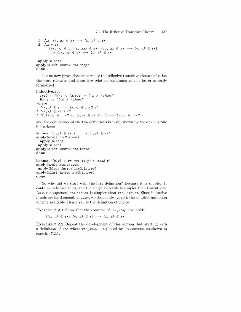
7.2 The Reflexive Transitive Closure 137
1.∧x. (x, z) ∈ r* −→ (x, z) ∈ r*
2.∧x y za.
[[(x, y) ∈ r; (y, za) ∈ r*; (za, z) ∈ r* −→ (y, z) ∈ r* ]]=⇒ (za, z) ∈ r* −→ (x, z) ∈ r*
apply(blast)apply(blast intro: rtc_step)done
Let us now prove that r* is really the reflexive transitive closure of r, i.e.the least reflexive and transitive relation containing r. The latter is easilyformalized
inductive setrtc2 :: "(’a × ’a)set ⇒ (’a × ’a)set"for r :: "(’a × ’a)set"
where"(x,y) ∈ r =⇒ (x,y) ∈ rtc2 r"
| "(x,x) ∈ rtc2 r"| " [[ (x,y) ∈ rtc2 r; (y,z) ∈ rtc2 r ]] =⇒ (x,z) ∈ rtc2 r"
and the equivalence of the two definitions is easily shown by the obvious ruleinductions:
lemma "(x,y) ∈ rtc2 r =⇒ (x,y) ∈ r*"apply(erule rtc2.induct)
apply(blast)apply(blast)
apply(blast intro: rtc_trans)done
lemma "(x,y) ∈ r* =⇒ (x,y) ∈ rtc2 r"apply(erule rtc.induct)apply(blast intro: rtc2.intros)
apply(blast intro: rtc2.intros)done
So why did we start with the first definition? Because it is simpler. Itcontains only two rules, and the single step rule is simpler than transitivity.As a consequence, rtc.induct is simpler than rtc2.induct. Since inductiveproofs are hard enough anyway, we should always pick the simplest inductionschema available. Hence rtc is the definition of choice.
Exercise 7.2.1 Show that the converse of rtc_step also holds:
[[(x, y) ∈ r*; (y, z) ∈ r ]] =⇒ (x, z) ∈ r*
Exercise 7.2.2 Repeat the development of this section, but starting witha definition of rtc where rtc_step is replaced by its converse as shown inexercise 7.2.1.
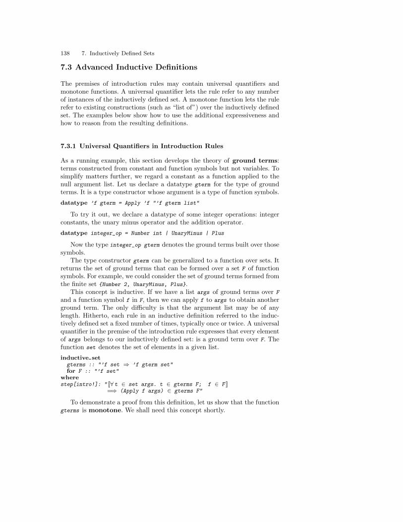
138 7. Inductively Defined Sets
7.3 Advanced Inductive Definitions
The premises of introduction rules may contain universal quantifiers andmonotone functions. A universal quantifier lets the rule refer to any numberof instances of the inductively defined set. A monotone function lets the rulerefer to existing constructions (such as “list of”) over the inductively definedset. The examples below show how to use the additional expressiveness andhow to reason from the resulting definitions.
7.3.1 Universal Quantifiers in Introduction Rules
As a running example, this section develops the theory of ground terms:terms constructed from constant and function symbols but not variables. Tosimplify matters further, we regard a constant as a function applied to thenull argument list. Let us declare a datatype gterm for the type of groundterms. It is a type constructor whose argument is a type of function symbols.
datatype ’f gterm = Apply ’f "’f gterm list"
To try it out, we declare a datatype of some integer operations: integerconstants, the unary minus operator and the addition operator.
datatype integer_op = Number int | UnaryMinus | Plus
Now the type integer_op gterm denotes the ground terms built over thosesymbols.
The type constructor gterm can be generalized to a function over sets. Itreturns the set of ground terms that can be formed over a set F of functionsymbols. For example, we could consider the set of ground terms formed fromthe finite set {Number 2, UnaryMinus, Plus}.
This concept is inductive. If we have a list args of ground terms over F
and a function symbol f in F, then we can apply f to args to obtain anotherground term. The only difficulty is that the argument list may be of anylength. Hitherto, each rule in an inductive definition referred to the induc-tively defined set a fixed number of times, typically once or twice. A universalquantifier in the premise of the introduction rule expresses that every elementof args belongs to our inductively defined set: is a ground term over F. Thefunction set denotes the set of elements in a given list.
inductive setgterms :: "’f set ⇒ ’f gterm set"for F :: "’f set"
wherestep[intro!]: " [[∀ t ∈ set args. t ∈ gterms F; f ∈ F ]]
=⇒ (Apply f args) ∈ gterms F"
To demonstrate a proof from this definition, let us show that the functiongterms is monotone. We shall need this concept shortly.
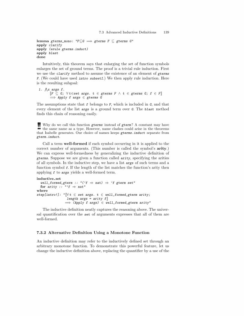
7.3 Advanced Inductive Definitions 139
lemma gterms_mono: "F⊆G =⇒ gterms F ⊆ gterms G"apply clarifyapply (erule gterms.induct)apply blastdone
Intuitively, this theorem says that enlarging the set of function symbolsenlarges the set of ground terms. The proof is a trivial rule induction. Firstwe use the clarify method to assume the existence of an element of gtermsF. (We could have used intro subsetI.) We then apply rule induction. Hereis the resulting subgoal:
1.∧x args f.
[[F ⊆ G; ∀ t∈set args. t ∈ gterms F ∧ t ∈ gterms G; f ∈ F ]]=⇒ Apply f args ∈ gterms G
The assumptions state that f belongs to F, which is included in G, and thatevery element of the list args is a ground term over G. The blast methodfinds this chain of reasoning easily.
!! Why do we call this function gterms instead of gterm? A constant may havethe same name as a type. However, name clashes could arise in the theorems
that Isabelle generates. Our choice of names keeps gterms.induct separate fromgterm.induct.
Call a term well-formed if each symbol occurring in it is applied to thecorrect number of arguments. (This number is called the symbol’s arity.)We can express well-formedness by generalizing the inductive definition ofgterms. Suppose we are given a function called arity, specifying the aritiesof all symbols. In the inductive step, we have a list args of such terms and afunction symbol f. If the length of the list matches the function’s arity thenapplying f to args yields a well-formed term.
inductive setwell_formed_gterm :: "(’f ⇒ nat) ⇒ ’f gterm set"for arity :: "’f ⇒ nat"
wherestep[intro!]: " [[∀ t ∈ set args. t ∈ well_formed_gterm arity;
length args = arity f ]]=⇒ (Apply f args) ∈ well_formed_gterm arity"
The inductive definition neatly captures the reasoning above. The univer-sal quantification over the set of arguments expresses that all of them arewell-formed.
7.3.2 Alternative Definition Using a Monotone Function
An inductive definition may refer to the inductively defined set through anarbitrary monotone function. To demonstrate this powerful feature, let uschange the inductive definition above, replacing the quantifier by a use of the
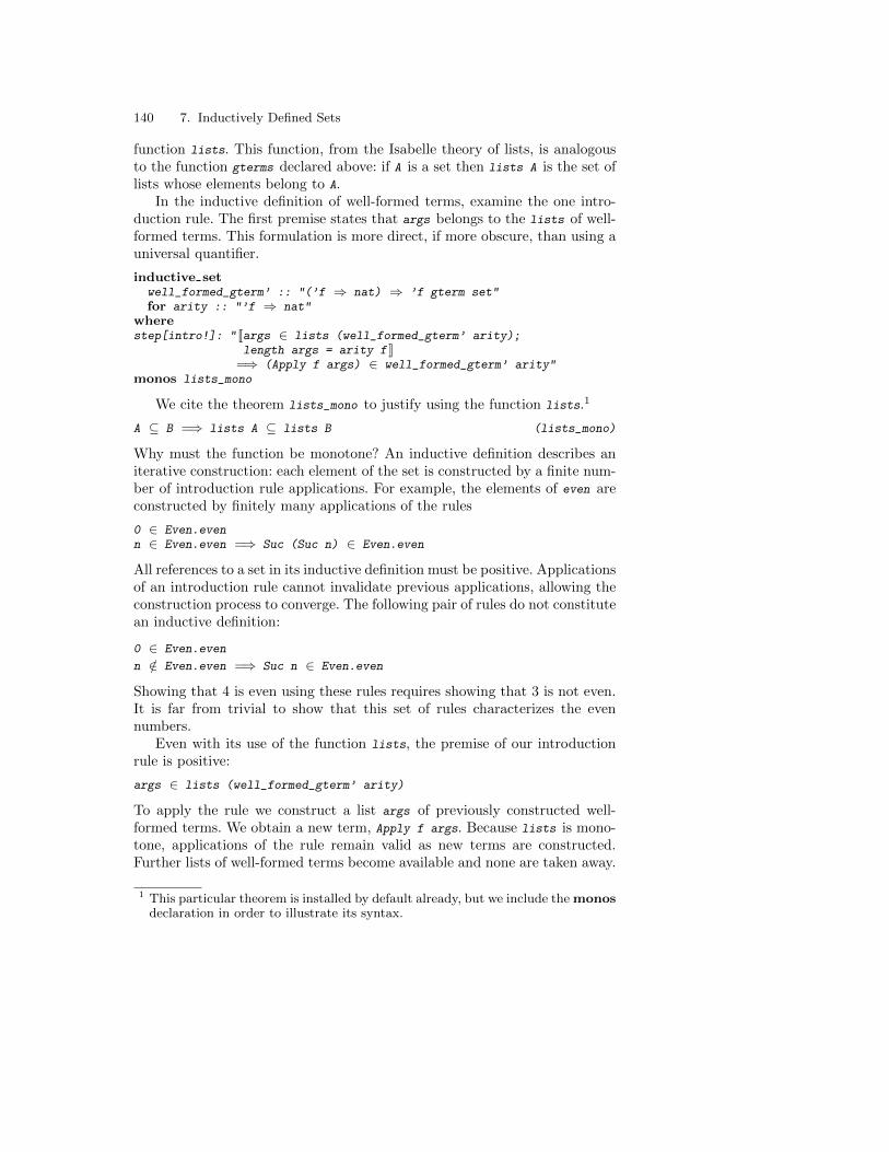
140 7. Inductively Defined Sets
function lists. This function, from the Isabelle theory of lists, is analogousto the function gterms declared above: if A is a set then lists A is the set oflists whose elements belong to A.
In the inductive definition of well-formed terms, examine the one intro-duction rule. The first premise states that args belongs to the lists of well-formed terms. This formulation is more direct, if more obscure, than using auniversal quantifier.
inductive setwell_formed_gterm’ :: "(’f ⇒ nat) ⇒ ’f gterm set"for arity :: "’f ⇒ nat"
wherestep[intro!]: " [[args ∈ lists (well_formed_gterm’ arity);
length args = arity f ]]=⇒ (Apply f args) ∈ well_formed_gterm’ arity"
monos lists_mono
We cite the theorem lists_mono to justify using the function lists.1
A ⊆ B =⇒ lists A ⊆ lists B (lists_mono)
Why must the function be monotone? An inductive definition describes aniterative construction: each element of the set is constructed by a finite num-ber of introduction rule applications. For example, the elements of even areconstructed by finitely many applications of the rules
0 ∈ Even.evenn ∈ Even.even =⇒ Suc (Suc n) ∈ Even.even
All references to a set in its inductive definition must be positive. Applicationsof an introduction rule cannot invalidate previous applications, allowing theconstruction process to converge. The following pair of rules do not constitutean inductive definition:
0 ∈ Even.even
n /∈ Even.even =⇒ Suc n ∈ Even.even
Showing that 4 is even using these rules requires showing that 3 is not even.It is far from trivial to show that this set of rules characterizes the evennumbers.
Even with its use of the function lists, the premise of our introductionrule is positive:
args ∈ lists (well_formed_gterm’ arity)
To apply the rule we construct a list args of previously constructed well-formed terms. We obtain a new term, Apply f args. Because lists is mono-tone, applications of the rule remain valid as new terms are constructed.Further lists of well-formed terms become available and none are taken away.
1 This particular theorem is installed by default already, but we include the monosdeclaration in order to illustrate its syntax.
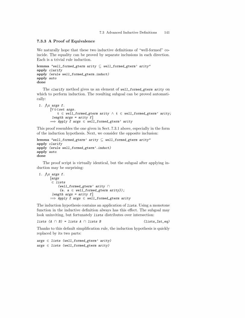
7.3 Advanced Inductive Definitions 141
7.3.3 A Proof of Equivalence
We naturally hope that these two inductive definitions of “well-formed” co-incide. The equality can be proved by separate inclusions in each direction.Each is a trivial rule induction.
lemma "well_formed_gterm arity ⊆ well_formed_gterm’ arity"apply clarifyapply (erule well_formed_gterm.induct)apply autodone
The clarify method gives us an element of well_formed_gterm arity onwhich to perform induction. The resulting subgoal can be proved automati-cally:
1.∧x args f.
[[∀ t∈set args.t ∈ well_formed_gterm arity ∧ t ∈ well_formed_gterm’ arity;
length args = arity f ]]=⇒ Apply f args ∈ well_formed_gterm’ arity
This proof resembles the one given in Sect. 7.3.1 above, especially in the formof the induction hypothesis. Next, we consider the opposite inclusion:
lemma "well_formed_gterm’ arity ⊆ well_formed_gterm arity"apply clarifyapply (erule well_formed_gterm’.induct)apply autodone
The proof script is virtually identical, but the subgoal after applying in-duction may be surprising:
1.∧x args f.
[[args∈ lists
(well_formed_gterm’ arity ∩{a. a ∈ well_formed_gterm arity});
length args = arity f ]]=⇒ Apply f args ∈ well_formed_gterm arity
The induction hypothesis contains an application of lists. Using a monotonefunction in the inductive definition always has this effect. The subgoal maylook uninviting, but fortunately lists distributes over intersection:
lists (A ∩ B) = lists A ∩ lists B (lists_Int_eq)
Thanks to this default simplification rule, the induction hypothesis is quicklyreplaced by its two parts:
args ∈ lists (well_formed_gterm’ arity)
args ∈ lists (well_formed_gterm arity)
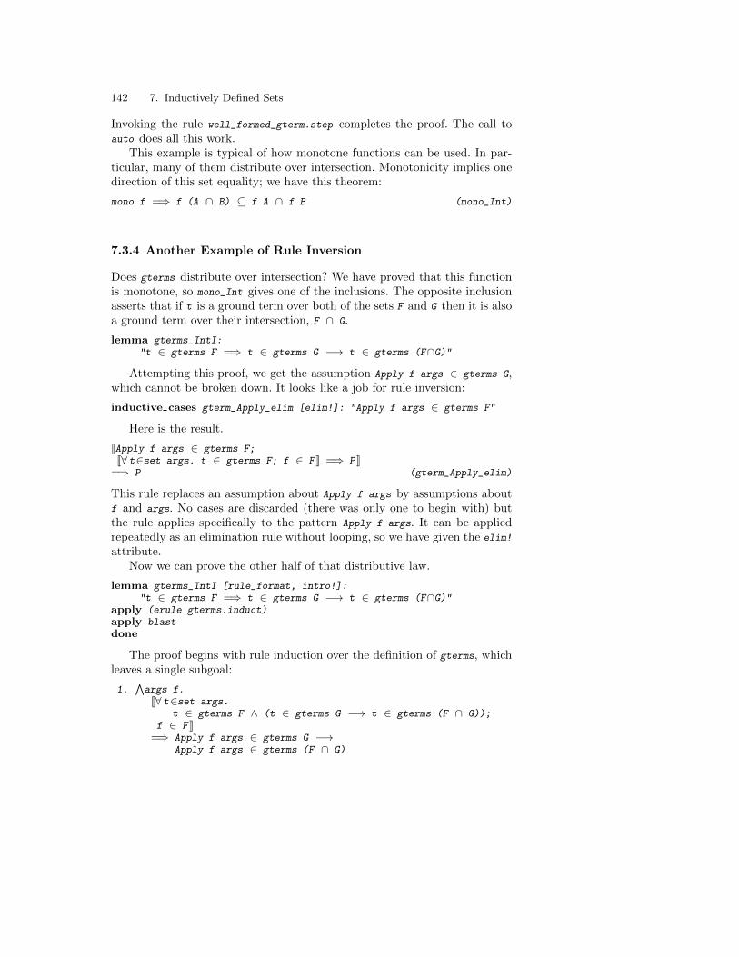
142 7. Inductively Defined Sets
Invoking the rule well_formed_gterm.step completes the proof. The call toauto does all this work.
This example is typical of how monotone functions can be used. In par-ticular, many of them distribute over intersection. Monotonicity implies onedirection of this set equality; we have this theorem:
mono f =⇒ f (A ∩ B) ⊆ f A ∩ f B (mono_Int)
7.3.4 Another Example of Rule Inversion
Does gterms distribute over intersection? We have proved that this functionis monotone, so mono_Int gives one of the inclusions. The opposite inclusionasserts that if t is a ground term over both of the sets F and G then it is alsoa ground term over their intersection, F ∩ G.
lemma gterms_IntI:"t ∈ gterms F =⇒ t ∈ gterms G −→ t ∈ gterms (F∩G)"
Attempting this proof, we get the assumption Apply f args ∈ gterms G,which cannot be broken down. It looks like a job for rule inversion:
inductive cases gterm_Apply_elim [elim!]: "Apply f args ∈ gterms F"
Here is the result.
[[Apply f args ∈ gterms F;[[∀ t∈set args. t ∈ gterms F; f ∈ F ]] =⇒ P ]]
=⇒ P (gterm_Apply_elim)
This rule replaces an assumption about Apply f args by assumptions aboutf and args. No cases are discarded (there was only one to begin with) butthe rule applies specifically to the pattern Apply f args. It can be appliedrepeatedly as an elimination rule without looping, so we have given the elim!
attribute.Now we can prove the other half of that distributive law.
lemma gterms_IntI [rule_format, intro!]:"t ∈ gterms F =⇒ t ∈ gterms G −→ t ∈ gterms (F∩G)"
apply (erule gterms.induct)apply blastdone
The proof begins with rule induction over the definition of gterms, whichleaves a single subgoal:
1.∧args f.
[[∀ t∈set args.t ∈ gterms F ∧ (t ∈ gterms G −→ t ∈ gterms (F ∩ G));
f ∈ F ]]=⇒ Apply f args ∈ gterms G −→
Apply f args ∈ gterms (F ∩ G)
7.4 Case Study: A Context Free Grammar 143
To prove this, we assume Apply f args ∈ gterms G. Rule inversion, in theform of gterm_Apply_elim, infers that every element of args belongs to gterms
G ; hence (by the induction hypothesis) it belongs to gterms (F ∩ G). Ruleinversion also yields f ∈ G and hence f ∈ F ∩ G. All of this reasoning isdone by blast.
Our distributive law is a trivial consequence of previously-proved results:
lemma gterms_Int_eq [simp]:"gterms (F ∩ G) = gterms F ∩ gterms G"
by (blast intro!: mono_Int monoI gterms_mono)
Exercise 7.3.1 A function mapping function symbols to their types is calleda signature. Given a type ranging over type symbols, we can represent afunction’s type by a list of argument types paired with the result type. Com-plete this inductive definition:
inductive setwell_typed_gterm :: "(’f ⇒ ’t list * ’t) ⇒ (’f gterm * ’t)set"for sig :: "’f ⇒ ’t list * ’t"
7.4 Case Study: A Context Free Grammar
Grammars are nothing but shorthands for inductive definitions of nontermi-nals which represent sets of strings. For example, the production A→ Bc isshort for
w ∈ B =⇒ wc ∈ A
This section demonstrates this idea with an example due to Hopcroft andUllman, a grammar for generating all words with an equal number of a’sand b’s:
S → ε | bA | aB
A → aS | bAA
B → bS | aBB
At the end we say a few words about the relationship between the originalproof [14, p. 81] and our formal version.
We start by fixing the alphabet, which consists only of a ’s and b ’s:
datatype alfa = a | b
For convenience we include the following easy lemmas as simplification rules:
lemma [simp]: "(x 6= a) = (x = b) ∧ (x 6= b) = (x = a)"by (case_tac x, auto)
144 7. Inductively Defined Sets
Words over this alphabet are of type alfa list, and the three nonterminalsare declared as sets of such words. The productions above are recast as amutual inductive definition of S, A and B :
inductive setS :: "alfa list set" andA :: "alfa list set" andB :: "alfa list set"
where"[] ∈ S"
| "w ∈ A =⇒ b#w ∈ S"| "w ∈ B =⇒ a#w ∈ S"
| "w ∈ S =⇒ a#w ∈ A"| " [[ v∈A; w∈A ]] =⇒ b#v@w ∈ A"
| "w ∈ S =⇒ b#w ∈ B"| " [[ v ∈ B; w ∈ B ]] =⇒ a#v@w ∈ B"
First we show that all words in S contain the same number of a ’s and b ’s.Since the definition of S is by mutual induction, so is the proof: we show atthe same time that all words in A contain one more a than b and all wordsin B contain one more b than a.
lemma correctness:"(w ∈ S −→ size[x←w. x=a] = size[x←w. x=b]) ∧(w ∈ A −→ size[x←w. x=a] = size[x←w. x=b] + 1) ∧(w ∈ B −→ size[x←w. x=b] = size[x←w. x=a] + 1)"
These propositions are expressed with the help of the predefined filter func-tion on lists, which has the convenient syntax [x←xs. P x], the list of all el-ements x in xs such that P x holds. Remember that on lists size and length
are synonymous.The proof itself is by rule induction and afterwards automatic:
by (rule S_A_B.induct, auto)
This may seem surprising at first, and is indeed an indication of the powerof inductive definitions. But it is also quite straightforward. For example,consider the production A→ bAA: if v ,w ∈ A and the elements of A containone more a than b’s, then bvw must again contain one more a than b’s.
As usual, the correctness of syntactic descriptions is easy, but complete-ness is hard: does S contain all words with an equal number of a ’s and b ’s? Itturns out that this proof requires the following lemma: every string with twomore a ’s than b ’s can be cut somewhere such that each half has one more a
than b. This is best seen by imagining counting the difference between thenumber of a ’s and b ’s starting at the left end of the word. We start with0 and end (at the right end) with 2. Since each move to the right increasesor decreases the difference by 1, we must have passed through 1 on our wayfrom 0 to 2. Formally, we appeal to the following discrete intermediate valuetheorem nat0_intermed_int_val
7.4 Case Study: A Context Free Grammar 145
[[∀ i<n. |f (i + 1) - f i | ≤ 1; f 0 ≤ k; k ≤ f n ]]=⇒ ∃ i≤n. f i = k
where f is of type nat ⇒ int, int are the integers, |. | is the absolute valuefunction2, and 1 is the integer 1 (see Sect. 8.4).
First we show that our specific function, the difference between the num-bers of a ’s and b ’s, does indeed only change by 1 in every move to the right.At this point we also start generalizing from a ’s and b ’s to an arbitrary prop-erty P. Otherwise we would have to prove the desired lemma twice, once asstated above and once with the roles of a ’s and b ’s interchanged.
lemma step1: "∀ i < size w.|(int(size[x←take (i+1) w. P x])-int(size[x←take (i+1) w. ¬P x]))- (int(size[x←take i w. P x])-int(size[x←take i w. ¬P x])) | ≤ 1"
The lemma is a bit hard to read because of the coercion function int :: nat
⇒ int. It is required because size returns a natural number, but subtractionon type nat will do the wrong thing. Function take is predefined and take
i xs is the prefix of length i of xs ; below we also need drop i xs, which iswhat remains after that prefix has been dropped from xs.
The proof is by induction on w, with a trivial base case, and a not so trivialinduction step. Since it is essentially just arithmetic, we do not discuss it.
apply(induct_tac w)apply(auto simp add: abs_if take_Cons split: nat.split)done
Finally we come to the above-mentioned lemma about cutting in half aword with two more elements of one sort than of the other sort:
lemma part1:"size[x←w. P x] = size[x←w. ¬P x]+2 =⇒∃ i≤size w. size[x←take i w. P x] = size[x←take i w. ¬P x]+1"
This is proved by force with the help of the intermediate value theorem,instantiated appropriately and with its first premise disposed of by lemmastep1 :
apply(insert nat0_intermed_int_val[OF step1, of "P" "w" "1"])by force
Lemma part1 tells us only about the prefix take i w. An easy lemmadeals with the suffix drop i w :
lemma part2:" [[size[x←take i w @ drop i w. P x] =
size[x←take i w @ drop i w. ¬P x]+2;size[x←take i w. P x] = size[x←take i w. ¬P x]+1 ]]
=⇒ size[x←drop i w. P x] = size[x←drop i w. ¬P x]+1"by(simp del: append_take_drop_id)
In the proof we have disabled the normally useful lemma
2 See Table A.1 in the Appendix for the correct ascii syntax.
146 7. Inductively Defined Sets
take n xs @ drop n xs = xs (append_take_drop_id)
to allow the simplifier to apply the following lemma instead:
[x∈xs@ys. P x] = [x∈xs. P x] @ [x∈ys. P x]
To dispose of trivial cases automatically, the rules of the inductive defini-tion are declared simplification rules:
declare S_A_B.intros[simp]
This could have been done earlier but was not necessary so far.The completeness theorem tells us that if a word has the same number of
a ’s and b ’s, then it is in S, and similarly for A and B :
theorem completeness:"(size[x←w. x=a] = size[x←w. x=b] −→ w ∈ S) ∧(size[x←w. x=a] = size[x←w. x=b] + 1 −→ w ∈ A) ∧(size[x←w. x=b] = size[x←w. x=a] + 1 −→ w ∈ B)"
The proof is by induction on w. Structural induction would fail here because,as we can see from the grammar, we need to make bigger steps than merelyappending a single letter at the front. Hence we induct on the length of w,using the induction rule length_induct :
apply(induct_tac w rule: length_induct)apply(rename_tac w)
The rule parameter tells induct_tac explicitly which induction rule to use.For details see Sect. 9.2.2 below. In this case the result is that we may assumethe lemma already holds for all words shorter than w. Because the inductionstep renames the induction variable we rename it back to w.
The proof continues with a case distinction on w, on whether w is emptyor not.
apply(case_tac w)apply(simp_all)
Simplification disposes of the base case and leaves only a conjunction of twostep cases to be proved: if w = a # v and
length (if x = a then [x ∈ v] else []) =length (if x = b then [x ∈ v] else []) + 2
then b # v ∈ A, and similarly for w = b # v. We only consider the first casein detail.
After breaking the conjunction up into two cases, we can apply part1 tothe assumption that w contains two more a ’s than b ’s.
apply(rule conjI)apply(clarify)apply(frule part1[of "λx. x=a", simplified])apply(clarify)
This yields an index i ≤ length v such that
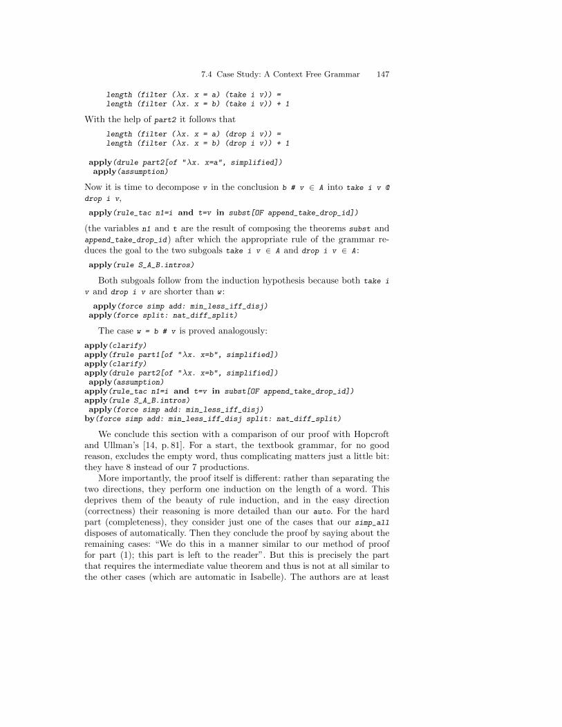
7.4 Case Study: A Context Free Grammar 147
length (filter (λx. x = a) (take i v)) =length (filter (λx. x = b) (take i v)) + 1
With the help of part2 it follows that
length (filter (λx. x = a) (drop i v)) =length (filter (λx. x = b) (drop i v)) + 1
apply(drule part2[of "λx. x=a", simplified])apply(assumption)
Now it is time to decompose v in the conclusion b # v ∈ A into take i v @
drop i v,
apply(rule_tac n1=i and t=v in subst[OF append_take_drop_id])
(the variables n1 and t are the result of composing the theorems subst andappend_take_drop_id) after which the appropriate rule of the grammar re-duces the goal to the two subgoals take i v ∈ A and drop i v ∈ A :
apply(rule S_A_B.intros)
Both subgoals follow from the induction hypothesis because both take i
v and drop i v are shorter than w :
apply(force simp add: min_less_iff_disj)apply(force split: nat_diff_split)
The case w = b # v is proved analogously:
apply(clarify)apply(frule part1[of "λx. x=b", simplified])apply(clarify)apply(drule part2[of "λx. x=b", simplified])apply(assumption)
apply(rule_tac n1=i and t=v in subst[OF append_take_drop_id])apply(rule S_A_B.intros)apply(force simp add: min_less_iff_disj)
by(force simp add: min_less_iff_disj split: nat_diff_split)
We conclude this section with a comparison of our proof with Hopcroftand Ullman’s [14, p. 81]. For a start, the textbook grammar, for no goodreason, excludes the empty word, thus complicating matters just a little bit:they have 8 instead of our 7 productions.
More importantly, the proof itself is different: rather than separating thetwo directions, they perform one induction on the length of a word. Thisdeprives them of the beauty of rule induction, and in the easy direction(correctness) their reasoning is more detailed than our auto. For the hardpart (completeness), they consider just one of the cases that our simp_all
disposes of automatically. Then they conclude the proof by saying about theremaining cases: “We do this in a manner similar to our method of prooffor part (1); this part is left to the reader”. But this is precisely the partthat requires the intermediate value theorem and thus is not at all similar tothe other cases (which are automatic in Isabelle). The authors are at least

148 7. Inductively Defined Sets
cavalier about this point and may even have overlooked the slight difficultylurking in the omitted cases. Such errors are found in many pen-and-paperproofs when they are scrutinized formally.

Part III
Advanced Material

8. More about Types
So far we have learned about a few basic types (for example bool and nat),type abbreviations (types) and recursive datatypes (datatype). This chap-ter will introduce more advanced material:
– Pairs (Sect. 8.1) and records (Sect. 8.2), and how to reason about them.– Type classes: how to specify and reason about axiomatic collections of
types (Sect. 8.3). This section leads on to a discussion of Isabelle’s numerictypes (Sect. 8.4).
– Introducing your own types: how to define types that cannot be constructedwith any of the basic methods (Sect. 8.5).
The material in this section goes beyond the needs of most novices. Serioususers should at least skim the sections as far as type classes. That materialis fairly advanced; read the beginning to understand what it is about, butconsult the rest only when necessary.
8.1 Pairs and Tuples
Ordered pairs were already introduced in Sect. 2.6.2, but only with a minimalrepertoire of operations: pairing and the two projections fst and snd. Inany non-trivial application of pairs you will find that this quickly leads tounreadable nests of projections. This section introduces syntactic sugar toovercome this problem: pattern matching with tuples.
8.1.1 Pattern Matching with Tuples
Tuples may be used as patterns in λ-abstractions, for example λ(x,y,z).x+y+zand λ((x,y),z).x+y+z. In fact, tuple patterns can be used in most variablebinding constructs, and they can be nested. Here are some typical examples:
let (x, y) = f z in (y, x)
case xs of [] ⇒ 0 | (x, y) # zs ⇒ x + y
∀ (x,y)∈A. x=y
{(x,y,z). x=z}⋃(x, y)∈A {x + y}
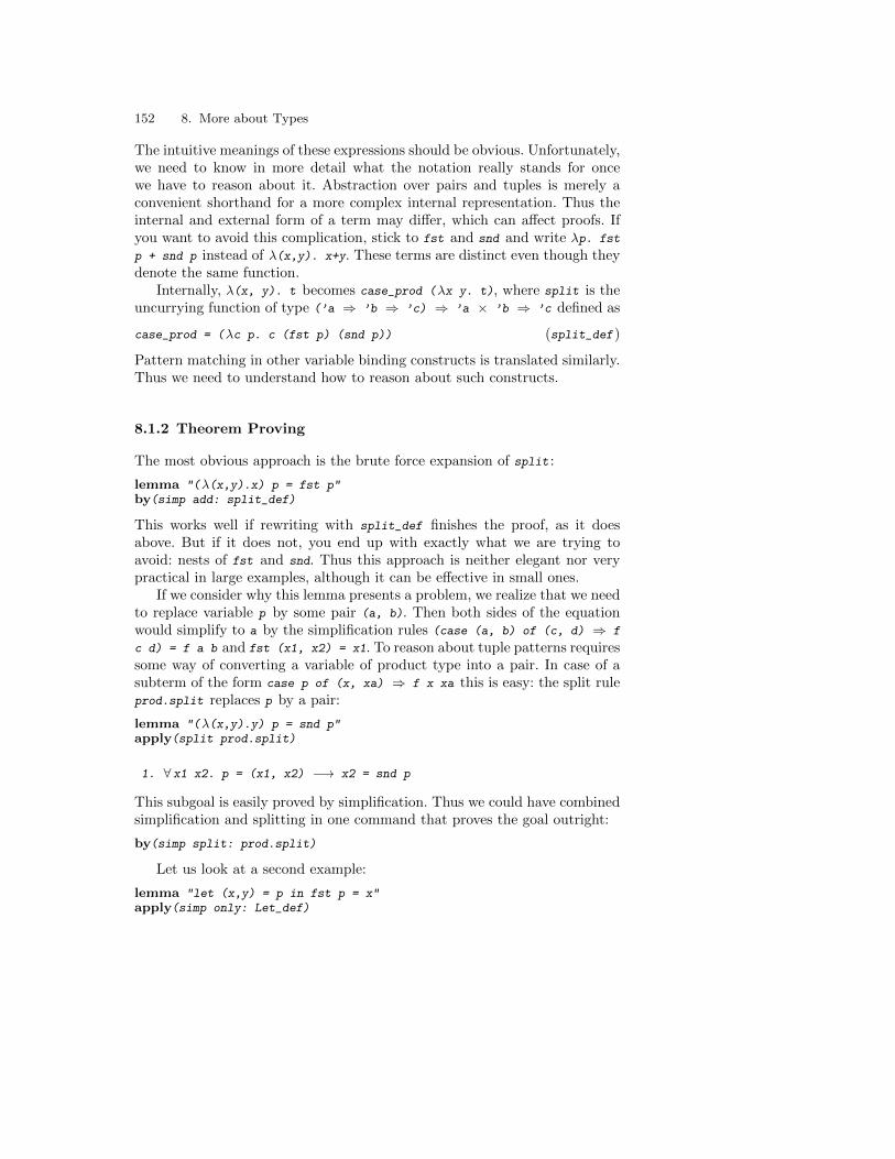
152 8. More about Types
The intuitive meanings of these expressions should be obvious. Unfortunately,we need to know in more detail what the notation really stands for oncewe have to reason about it. Abstraction over pairs and tuples is merely aconvenient shorthand for a more complex internal representation. Thus theinternal and external form of a term may differ, which can affect proofs. Ifyou want to avoid this complication, stick to fst and snd and write λp. fst
p + snd p instead of λ(x,y). x+y. These terms are distinct even though theydenote the same function.
Internally, λ(x, y). t becomes case_prod (λx y. t), where split is theuncurrying function of type (’a ⇒ ’b ⇒ ’c) ⇒ ’a × ’b ⇒ ’c defined as
case_prod = (λc p. c (fst p) (snd p)) (split_def)
Pattern matching in other variable binding constructs is translated similarly.Thus we need to understand how to reason about such constructs.
8.1.2 Theorem Proving
The most obvious approach is the brute force expansion of split :
lemma "(λ(x,y).x) p = fst p"by(simp add: split_def)
This works well if rewriting with split_def finishes the proof, as it doesabove. But if it does not, you end up with exactly what we are trying toavoid: nests of fst and snd. Thus this approach is neither elegant nor verypractical in large examples, although it can be effective in small ones.
If we consider why this lemma presents a problem, we realize that we needto replace variable p by some pair (a, b). Then both sides of the equationwould simplify to a by the simplification rules (case (a, b) of (c, d) ⇒ f
c d) = f a b and fst (x1, x2) = x1. To reason about tuple patterns requiressome way of converting a variable of product type into a pair. In case of asubterm of the form case p of (x, xa) ⇒ f x xa this is easy: the split ruleprod.split replaces p by a pair:
lemma "(λ(x,y).y) p = snd p"apply(split prod.split)
1. ∀ x1 x2. p = (x1, x2) −→ x2 = snd p
This subgoal is easily proved by simplification. Thus we could have combinedsimplification and splitting in one command that proves the goal outright:
by(simp split: prod.split)
Let us look at a second example:
lemma "let (x,y) = p in fst p = x"apply(simp only: Let_def)
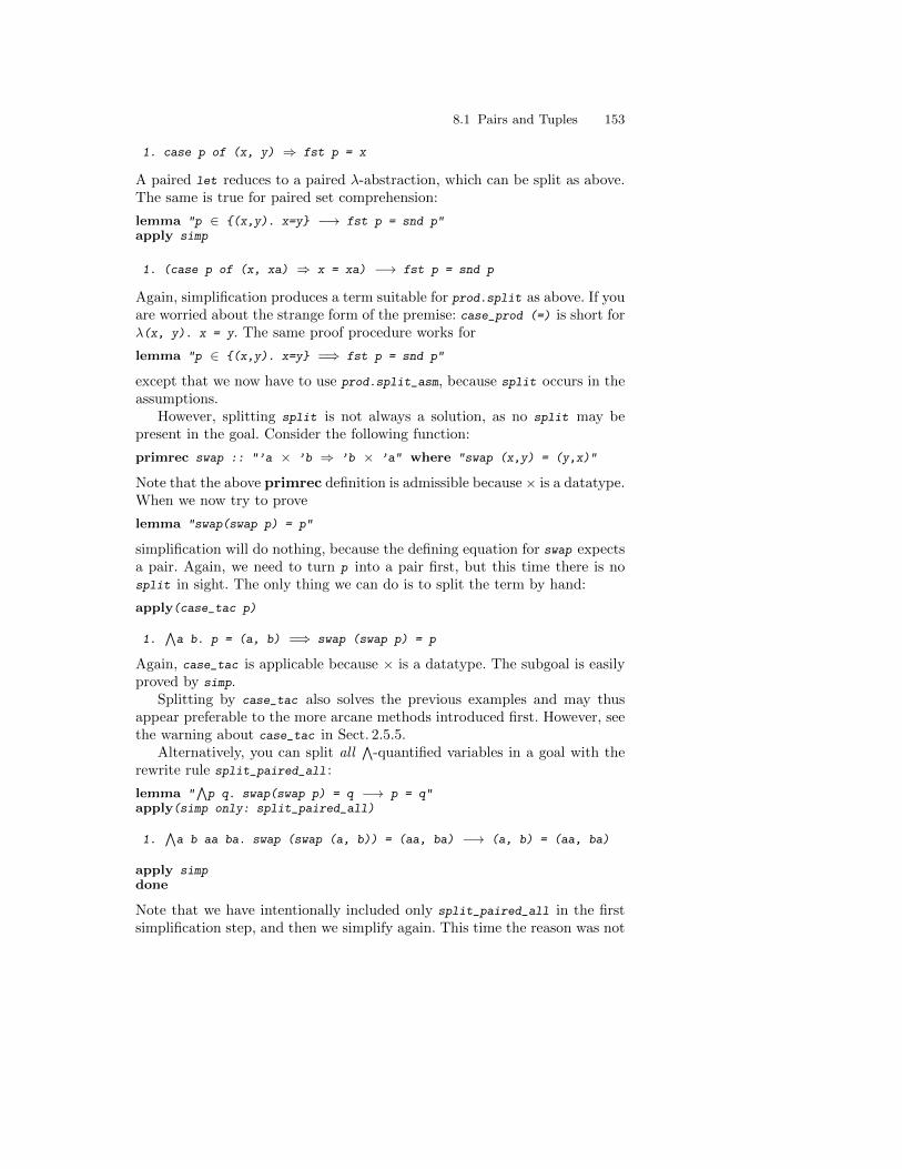
8.1 Pairs and Tuples 153
1. case p of (x, y) ⇒ fst p = x
A paired let reduces to a paired λ-abstraction, which can be split as above.The same is true for paired set comprehension:
lemma "p ∈ {(x,y). x=y} −→ fst p = snd p"apply simp
1. (case p of (x, xa) ⇒ x = xa) −→ fst p = snd p
Again, simplification produces a term suitable for prod.split as above. If youare worried about the strange form of the premise: case_prod (=) is short forλ(x, y). x = y. The same proof procedure works for
lemma "p ∈ {(x,y). x=y} =⇒ fst p = snd p"
except that we now have to use prod.split_asm, because split occurs in theassumptions.
However, splitting split is not always a solution, as no split may bepresent in the goal. Consider the following function:
primrec swap :: "’a × ’b ⇒ ’b × ’a" where "swap (x,y) = (y,x)"
Note that the above primrec definition is admissible because × is a datatype.When we now try to prove
lemma "swap(swap p) = p"
simplification will do nothing, because the defining equation for swap expectsa pair. Again, we need to turn p into a pair first, but this time there is nosplit in sight. The only thing we can do is to split the term by hand:
apply(case_tac p)
1.∧a b. p = (a, b) =⇒ swap (swap p) = p
Again, case_tac is applicable because × is a datatype. The subgoal is easilyproved by simp.
Splitting by case_tac also solves the previous examples and may thusappear preferable to the more arcane methods introduced first. However, seethe warning about case_tac in Sect. 2.5.5.
Alternatively, you can split all∧
-quantified variables in a goal with therewrite rule split_paired_all :
lemma "∧p q. swap(swap p) = q −→ p = q"
apply(simp only: split_paired_all)
1.∧a b aa ba. swap (swap (a, b)) = (aa, ba) −→ (a, b) = (aa, ba)
apply simpdone
Note that we have intentionally included only split_paired_all in the firstsimplification step, and then we simplify again. This time the reason was not
154 8. More about Types
merely pedagogical: split_paired_all may interfere with other functions ofthe simplifier. The following command could fail (here it does not) where twoseparate simp applications succeed.
apply(simp add: split_paired_all)
Finally, the simplifier automatically splits all ∀ and ∃ -quantified variables:
lemma "∀ p. ∃ q. swap p = swap q"by simp
To turn off this automatic splitting, disable the responsible simplificationrules:
(∀ x. P x) = (∀ a b. P (a, b)) (split_paired_All)(∃ x. P x) = (∃ a b. P (a, b)) (split_paired_Ex)
8.2 Records
Records are familiar from programming languages. A record of n fields isessentially an n-tuple, but the record’s components have names, which canmake expressions easier to read and reduces the risk of confusing one fieldfor another.
A record of Isabelle/HOL covers a collection of fields, with select andupdate operations. Each field has a specified type, which may be polymorphic.The field names are part of the record type, and the order of the fields issignificant — as it is in Pascal but not in Standard ML. If two differentrecord types have field names in common, then the ambiguity is resolved inthe usual way, by qualified names.
Record types can also be defined by extending other record types. Exten-sible records make use of the reserved pseudo-field more , which is present inevery record type. Generic record operations work on all possible extensionsof a given type scheme; polymorphism takes care of structural sub-typingbehind the scenes. There are also explicit coercion functions between fixedrecord types.
8.2.1 Record Basics
Record types are not primitive in Isabelle and have a delicate internal rep-resentation [22], based on nested copies of the primitive product type. Arecord declaration introduces a new record type scheme by specifying itsfields, which are packaged internally to hold up the perception of the recordas a distinguished entity. Here is a simple example:
record point =Xcoord :: int
8.2 Records 155
Ycoord :: int
Records of type point have two fields named Xcoord and Ycoord, both oftype int. We now define a constant of type point :
definition pt1 :: point where"pt1 ≡ (| Xcoord = 999, Ycoord = 23 |)"
We see above the ASCII notation for record brackets. You can also use thesymbolic brackets (| and |). Record type expressions can be also written di-rectly with individual fields. The type name above is merely an abbreviation.
definition pt2 :: "(|Xcoord :: int, Ycoord :: int |)" where"pt2 ≡ (|Xcoord = -45, Ycoord = 97 |)"
For each field, there is a selector function of the same name. For exam-ple, if p has type point then Xcoord p denotes the value of the Xcoord fieldof p. Expressions involving field selection of explicit records are simplifiedautomatically:
lemma "Xcoord (|Xcoord = a, Ycoord = b |) = a"by simp
The update operation is functional. For example, p(|Xcoord := 0 |) is arecord whose Xcoord value is zero and whose Ycoord value is copied from p.Updates of explicit records are also simplified automatically:
lemma "(|Xcoord = a, Ycoord = b |)(|Xcoord := 0 |) =(|Xcoord = 0, Ycoord = b |)"
by simp
!! Field names are declared as constants and can no longer be used as variables. Itwould be unwise, for example, to call the fields of type point simply x and y.
8.2.2 Extensible Records and Generic Operations
Now, let us define coloured points (type cpoint) to be points extended witha field col of type colour :
datatype colour = Red | Green | Blue
record cpoint = point +col :: colour
The fields of this new type are Xcoord, Ycoord and col, in that order.
definition cpt1 :: cpoint where"cpt1 ≡ (|Xcoord = 999, Ycoord = 23, col = Green |)"
We can define generic operations that work on arbitrary instances of arecord scheme, e.g. covering point, cpoint, and any further extensions. Everyrecord structure has an implicit pseudo-field, more , that keeps the extension
156 8. More about Types
as an explicit value. Its type is declared as completely polymorphic: ’a. Whena fixed record value is expressed using just its standard fields, the value ofmore is implicitly set to (), the empty tuple, which has type unit. Within therecord brackets, you can refer to the more field by writing “. . . ” (three dots):
lemma "Xcoord (|Xcoord = a, Ycoord = b, . . . = p |) = a"by simp
This lemma applies to any record whose first two fields are Xcoord
and Ycoord. Note that (|Xcoord = a, Ycoord = b, . . . = () |) is exactly thesame as (|Xcoord = a, Ycoord = b |). Selectors and updates are always poly-morphic wrt. the more part of a record scheme, its value is just ignored (forselect) or copied (for update).
The more pseudo-field may be manipulated directly as well, but the iden-tifier needs to be qualified:
lemma "point.more cpt1 = (|col = Green |)"by (simp add: cpt1_def)
We see that the colour part attached to this point is a rudimentary recordin its own right, namely (|col = Green |). In order to select or update col, thisfragment needs to be put back into the context of the parent type scheme,say as more part of another point.
To define generic operations, we need to know a bit more about records.Our definition of point above has generated two type abbreviations:
point = (|Xcoord :: int, Ycoord :: int |)’a point_scheme = (|Xcoord :: int, Ycoord :: int, . . . :: ’a |)
Type point is for fixed records having exactly the two fields Xcoord and Ycoord,while the polymorphic type ’a point_scheme comprises all possible extensionsto those two fields. Note that unit point_scheme coincides with point, and(|col :: colour |) point_scheme with cpoint.
In the following example we define two operations — methods, if we regardrecords as objects — to get and set any point’s Xcoord field.
definition getX :: "’a point_scheme ⇒ int" where"getX r ≡ Xcoord r"definition setX :: "’a point_scheme ⇒ int ⇒ ’a point_scheme" where"setX r a ≡ r(|Xcoord := a |)"
Here is a generic method that modifies a point, incrementing its Xcoord
field. The Ycoord and more fields are copied across. It works for any recordtype scheme derived from point (including cpoint etc.):
definition incX :: "’a point_scheme ⇒ ’a point_scheme" where"incX r ≡
(|Xcoord = Xcoord r + 1, Ycoord = Ycoord r, . . . = point.more r |)"
Generic theorems can be proved about generic methods. This triviallemma relates incX to getX and setX :
lemma "incX r = setX r (getX r + 1)"
8.2 Records 157
by (simp add: getX_def setX_def incX_def)
!! If you use the symbolic record brackets (| and |), then you must also use thesymbolic ellipsis, “. . . ”, rather than three consecutive periods, “...”. Mixing
the ASCII and symbolic versions causes a syntax error. (The two versions are moredistinct on screen than they are on paper.)
8.2.3 Record Equality
Two records are equal if all pairs of corresponding fields are equal. Concreterecord equalities are simplified automatically:
lemma "((|Xcoord = a, Ycoord = b |) = (|Xcoord = a’, Ycoord = b’ |)) =(a = a’ ∧ b = b’)"
by simp
The following equality is similar, but generic, in that r can be any instanceof ’a point_scheme :
lemma "r(|Xcoord := a, Ycoord := b |) = r(|Ycoord := b, Xcoord := a |)"by simp
We see above the syntax for iterated updates. We could equivalently havewritten the left-hand side as r(|Xcoord := a |)(|Ycoord := b |).
Record equality is extensional : a record is determined entirely by thevalues of its fields.
lemma "r = (|Xcoord = Xcoord r, Ycoord = Ycoord r |)"by simp
The generic version of this equality includes the pseudo-field more :
lemma "r = (|Xcoord = Xcoord r, Ycoord = Ycoord r, . . . = point.more r |)"by simp
The simplifier can prove many record equalities automatically, but generalequality reasoning can be tricky. Consider proving this obvious fact:
lemma "r(|Xcoord := a |) = r(|Xcoord := a’ |) =⇒ a = a’"apply simp?oops
Here the simplifier can do nothing, since general record equality is not elimi-nated automatically. One way to proceed is by an explicit forward step thatapplies the selector Xcoord to both sides of the assumed record equality:
lemma "r(|Xcoord := a |) = r(|Xcoord := a’ |) =⇒ a = a’"apply (drule_tac f = Xcoord in arg_cong)
1. Xcoord (r(|Xcoord := a |)) = Xcoord (r(|Xcoord := a’ |)) =⇒ a = a’
158 8. More about Types
Now, simp will reduce the assumption to the desired conclusion.
apply simpdone
The cases method is preferable to such a forward proof. We state thedesired lemma again:
lemma "r(|Xcoord := a |) = r(|Xcoord := a’ |) =⇒ a = a’"
The cases method adds an equality to replace the named record term byan explicit record expression, listing all fields. It even includes the pseudo-fieldmore, since the record equality stated here is generic for all extensions.
apply (cases r)
1.∧Xcoord Ycoord more.
[[r(|Xcoord := a |) = r(|Xcoord := a’ |);r = (|Xcoord = Xcoord, Ycoord = Ycoord, . . . = more |)]]
=⇒ a = a’
Again, simp finishes the proof. Because r is now represented as an explicitrecord construction, the updates can be applied and the record equality canbe replaced by equality of the corresponding fields (due to injectivity).
apply simpdone
The generic cases method does not admit references to locally boundparameters of a goal. In longer proof scripts one might have to fall back onthe primitive rule_tac used together with the internal field representationrules of records. The above use of (cases r) would become (rule_tac r = r
in point.cases_scheme).
8.2.4 Extending and Truncating Records
Each record declaration introduces a number of derived operations to refercollectively to a record’s fields and to convert between fixed record types.They can, for instance, convert between types point and cpoint. We can adda colour to a point or convert a cpoint to a point by forgetting its colour.
– Function make takes as arguments all of the record’s fields (including thoseinherited from ancestors). It returns the corresponding record.
– Function fields takes the record’s very own fields and returns a recordfragment consisting of just those fields. This may be filled into the more
part of the parent record scheme.– Function extend takes two arguments: a record to be extended and a record
containing the new fields.– Function truncate takes a record (possibly an extension of the original
record type) and returns a fixed record, removing any additional fields.
8.2 Records 159
These functions provide useful abbreviations for standard record expressionsinvolving constructors and selectors. The definitions, which are not unfoldedby default, are made available by the collective name of defs (point.defs,cpoint.defs, etc.). For example, here are the versions of those functions gen-erated for record point. We omit point.fields, which happens to be the sameas point.make.
point.make Xcoord Ycoord ≡ (|Xcoord = Xcoord, Ycoord = Ycoord |)point.extend r more ≡(|Xcoord = Xcoord r, Ycoord = Ycoord r, . . . = more |)point.truncate r ≡ (|Xcoord = Xcoord r, Ycoord = Ycoord r |)
Contrast those with the corresponding functions for record cpoint. Observecpoint.fields in particular.
cpoint.make Xcoord Ycoord col ≡(|Xcoord = Xcoord, Ycoord = Ycoord, col = col |)cpoint.fields col ≡ (|col = col |)cpoint.extend r more ≡(|Xcoord = Xcoord r, Ycoord = Ycoord r, col = col r, . . . = more |)cpoint.truncate r ≡(|Xcoord = Xcoord r, Ycoord = Ycoord r, col = col r |)
To demonstrate these functions, we declare a new coloured point byextending an ordinary point. Function point.extend augments pt1 with acolour value, which is converted into an appropriate record fragment bycpoint.fields.
definition cpt2 :: cpoint where"cpt2 ≡ point.extend pt1 (cpoint.fields Green)"
The coloured points cpt1 and cpt2 are equal. The proof is trivial, byunfolding all the definitions. We deliberately omit the definition of pt1 inorder to reveal the underlying comparison on type point.
lemma "cpt1 = cpt2"apply (simp add: cpt1_def cpt2_def point.defs cpoint.defs)
1. Xcoord pt1 = 999 ∧ Ycoord pt1 = 23
apply (simp add: pt1_def)done
In the example below, a coloured point is truncated to leave a point. Weuse the truncate function of the target record.
lemma "point.truncate cpt2 = pt1"by (simp add: pt1_def cpt2_def point.defs)
Exercise 8.2.1 Extend record cpoint to have a further field, intensity, oftype nat. Experiment with generic operations (using polymorphic selectorsand updates) and explicit coercions (using extend, truncate etc.) among thethree record types.
160 8. More about Types
Exercise 8.2.2 (For Java programmers.) Model a small class hierarchy usingrecords.
8.3 Type Classes
The programming language Haskell has popularized the notion of typeclasses: a type class is a set of types with a common interface: all typesin that class must provide the functions in the interface. Isabelle offers a sim-ilar type class concept: in addition, properties (class axioms) can be specifiedwhich any instance of this type class must obey. Thus we can talk about atype τ being in a class C , which is written τ :: C . This is the case if τ satisfiesthe axioms of C . Furthermore, type classes can be organized in a hierarchy.Thus there is the notion of a class D being a subclass of a class C , writtenD < C . This is the case if all axioms of C are also provable in D .
In this section we introduce the most important concepts behind typeclasses by means of a running example from algebra. This should give you anintuition how to use type classes and to understand specifications involvingtype classes. Type classes are covered more deeply in a separate tutorial [12].
8.3.1 Overloading
Type classes allow overloading ; thus a constant may have multiple definitionsat non-overlapping types.
Overloading. We can introduce a binary infix addition operator ⊕ for ar-bitrary types by means of a type class:
class plus =fixes plus :: "’a ⇒ ’a ⇒ ’a" ( infixl "⊕" 70)
This introduces a new class plus, along with a constant plus with nice infixsyntax. plus is also named class operation. The type of plus carries a classconstraint "’a :: plus" on its type variable, meaning that only types of classplus can be instantiated for "’a". To breathe life into plus we need to declarea type to be an instance of plus :
instantiation nat :: plusbegin
Command instantiation opens a local theory context. Here we can nowinstantiate plus on nat :
primrec plus_nat :: "nat ⇒ nat ⇒ nat" where"(0::nat) ⊕ n = n"
| "Suc m ⊕ n = Suc (m ⊕ n)"
8.3 Type Classes 161
Note that the name plus carries a suffix _nat ; by default, the local name of aclass operation f to be instantiated on type constructor κ is mangled as f_κ.In case of uncertainty, these names may be inspected using the print context
command.Although class plus has no axioms, the instantiation must be formally
concluded by a (trivial) instantiation proof “..”:
instance ..
More interesting instance proofs will arise below.The instantiation is finished by an explicit
end
From now on, terms like Suc (m ⊕ 2) are legal.
instantiation prod :: (plus, plus) plusbegin
Here we instantiate the product type prod to class plus, given that its typearguments are of class plus :
fun plus_prod :: "’a × ’b ⇒ ’a × ’b ⇒ ’a × ’b" where"(x, y) ⊕ (w, z) = (x ⊕ w, y ⊕ z)"
Obviously, overloaded specifications may include recursion over the syntacticstructure of types.
instance ..
end
This way we have encoded the canonical lifting of binary operations to prod-ucts by means of type classes.
8.3.2 Axioms
Attaching axioms to our classes lets us reason on the level of classes. Theresults will be applicable to all types in a class, just as in axiomatic mathe-matics.
!! Proofs in this section use structured Isar proofs, which are not covered in thistutorial; but see [25].
Semigroups. We specify semigroups as subclass of plus :
class semigroup = plus +assumes assoc: "(x ⊕ y) ⊕ z = x ⊕ (y ⊕ z)"
This class specification requires that all instances of semigroup obey assoc: "∧x
y z :: ’a::semigroup. (x ⊕ y) ⊕ z = x ⊕ (y ⊕ z)".
162 8. More about Types
We can use this class axiom to derive further abstract theorems relativeto class semigroup :
lemma assoc_left:fixes x y z :: "’a::semigroup"shows "x ⊕ (y ⊕ z) = (x ⊕ y) ⊕ z"using assoc by (rule sym)
The semigroup constraint on type ’a restricts instantiations of ’a to types ofclass semigroup and during the proof enables us to use the fact assoc whosetype parameter is itself constrained to class semigroup. The main advantageof classes is that theorems can be proved in the abstract and freely reusedfor each instance.
On instantiation, we have to give a proof that the given operations obeythe class axioms:
instantiation nat :: semigroupbegin
instance proof
The proof opens with a default proof step, which for instance judgementsinvokes method intro_classes .
fix m n q :: natshow "(m ⊕ n) ⊕ q = m ⊕ (n ⊕ q)"
by (induct m) simp_allqed
end
Again, the interesting things enter the stage with parametric types:
instantiation prod :: (semigroup, semigroup) semigroupbegin
instance prooffix p1 p2 p3 :: "’a::semigroup × ’b::semigroup"show "p1 ⊕ p2 ⊕ p3 = p1 ⊕ (p2 ⊕ p3)"
by (cases p1, cases p2, cases p3) (simp add: assoc)
Associativity of product semigroups is established using the hypothetical as-sociativity assoc of the type components, which holds due to the semigroup
constraints imposed on the type components by the instance proposition.Indeed, this pattern often occurs with parametric types and type classes.
qed
end
Monoids. We define a subclass monoidl (a semigroup with a left-hand neu-tral) by extending semigroup with one additional parameter neutral togetherwith its property:
class monoidl = semigroup +
8.3 Type Classes 163
fixes neutral :: "’a" ("0")assumes neutl: "0 ⊕ x = x"
Again, we prove some instances, by providing suitable parameter definitionsand proofs for the additional specifications.
instantiation nat :: monoidlbegin
definitionneutral_nat_def: "0 = (0::nat)"
instance prooffix n :: natshow "0 ⊕ n = n"
unfolding neutral_nat_def by simpqed
end
In contrast to the examples above, we here have both specification of classoperations and a non-trivial instance proof.
This covers products as well:
instantiation prod :: (monoidl, monoidl) monoidlbegin
definitionneutral_prod_def: "0 = (0, 0)"
instance prooffix p :: "’a::monoidl × ’b::monoidl"show "0 ⊕ p = p"
by (cases p) (simp add: neutral_prod_def neutl)qed
end
Fully-fledged monoids are modelled by another subclass which does not addnew parameters but tightens the specification:
class monoid = monoidl +assumes neutr: "x ⊕ 0 = x"
Corresponding instances for nat and products are left as an exercise to thereader.
Groups. To finish our small algebra example, we add a group class:
class group = monoidl +fixes inv :: "’a ⇒ ’a" ("÷ _" [81] 80)assumes invl: "÷ x ⊕ x = 0"
We continue with a further example for abstract proofs relative to typeclasses:
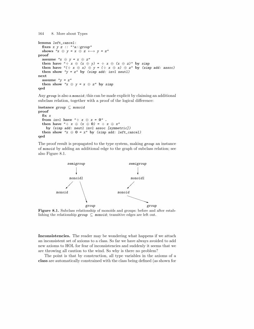
164 8. More about Types
lemma left_cancel:fixes x y z :: "’a::group"shows "x ⊕ y = x ⊕ z ←→ y = z"
proofassume "x ⊕ y = x ⊕ z"then have "÷ x ⊕ (x ⊕ y) = ÷ x ⊕ (x ⊕ z)" by simpthen have "(÷ x ⊕ x) ⊕ y = (÷ x ⊕ x) ⊕ z" by (simp add: assoc)then show "y = z" by (simp add: invl neutl)
nextassume "y = z"then show "x ⊕ y = x ⊕ z" by simp
qed
Any group is also a monoid ; this can be made explicit by claiming an additionalsubclass relation, together with a proof of the logical difference:
instance group ⊆ monoidproof
fix xfrom invl have "÷ x ⊕ x = 0" .then have "÷ x ⊕ (x ⊕ 0) = ÷ x ⊕ x"
by (simp add: neutl invl assoc [symmetric])then show "x ⊕ 0 = x" by (simp add: left_cancel)
qed
The proof result is propagated to the type system, making group an instanceof monoid by adding an additional edge to the graph of subclass relation; seealso Figure 8.1.
semigroup
monoidl
monoid
group
?
��
BBBBBBN
semigroup
monoidl
monoid
group
?
��
PPPPPPq
Figure 8.1. Subclass relationship of monoids and groups: before and after estab-lishing the relationship group ⊆ monoid ; transitive edges are left out.
Inconsistencies. The reader may be wondering what happens if we attachan inconsistent set of axioms to a class. So far we have always avoided to addnew axioms to HOL for fear of inconsistencies and suddenly it seems that weare throwing all caution to the wind. So why is there no problem?
The point is that by construction, all type variables in the axioms of aclass are automatically constrained with the class being defined (as shown for
8.4 Numbers 165
axiom refl above). These constraints are always carried around and Isabelletakes care that they are never lost, unless the type variable is instantiatedwith a type that has been shown to belong to that class. Thus you may beable to prove False from your axioms, but Isabelle will remind you that thistheorem has the hidden hypothesis that the class is non-empty.
Even if each individual class is consistent, intersections of (unrelated)classes readily become inconsistent in practice. Now we know this need notworry us.
Syntactic Classes and Predefined Overloading. In our algebra exam-ple, we have started with a syntactic class plus which only specifies opera-tions but no axioms; it would have been also possible to start immediatelywith class semigroup, specifying the ⊕ operation and associativity at the sametime.
Which approach is more appropriate depends. Usually it is more conve-nient to introduce operations and axioms in the same class: then the typechecker will automatically insert the corresponding class constraints when-ever the operations occur, reducing the need of manual annotations. However,when operations are decorated with popular syntax, syntactic classes can bean option to re-use the syntax in different contexts; this is indeed the waymost overloaded constants in HOL are introduced, of which the most impor-tant are listed in Table A.2 in the appendix. Section 8.4.5 covers a range ofcorresponding classes with axioms.
Further note that classes may contain axioms but no operations. An ex-ample is class finite from theory HOL.Finite_Set which specifies a type tobe finite: "finite (UNIV :: ’a::finite set)".
8.4 Numbers
Until now, our numerical examples have used the type of natural num-bers, nat. This is a recursive datatype generated by the constructors zeroand successor, so it works well with inductive proofs and primitive recursivefunction definitions. HOL also provides the type int of integers, which lackinduction but support true subtraction. With subtraction, arithmetic reason-ing is easier, which makes the integers preferable to the natural numbers forcomplicated arithmetic expressions, even if they are non-negative. There arealso the types rat, real and complex : the rational, real and complex num-bers. Isabelle has no subtyping, so the numeric types are distinct and thereare functions to convert between them. Most numeric operations are over-loaded: the same symbol can be used at all numeric types. Table A.2 in theappendix shows the most important operations, together with the prioritiesof the infix symbols. Algebraic properties are organized using type classesaround algebraic concepts such as rings and fields; a property such as the
166 8. More about Types
commutativity of addition is a single theorem (add.commute) that applies toall numeric types.
Many theorems involving numeric types can be proved automatically byIsabelle’s arithmetic decision procedure, the method arith . Linear arithmeticcomprises addition, subtraction and multiplication by constant factors; sub-terms involving other operators are regarded as variables. The procedure canbe slow, especially if the subgoal to be proved involves subtraction over typenat, which causes case splits. On types nat and int, arith can deal withquantifiers—this is known as Presburger arithmetic—whereas on type real
it cannot.The simplifier reduces arithmetic expressions in other ways, such as di-
viding through by common factors. For problems that lie outside the scopeof automation, HOL provides hundreds of theorems about multiplication, di-vision, etc., that can be brought to bear. You can locate them using ProofGeneral’s Find button. A few lemmas are given below to show what is avail-able.
8.4.1 Numeric Literals
The constants 0 and 1 are overloaded. They denote zero and one, respectively,for all numeric types. Other values are expressed by numeric literals, whichconsist of one or more decimal digits optionally preceeded by a minus sign(-). Examples are 2, -3 and 441223334678. Literals are available for the typesof natural numbers, integers, rationals, reals, etc.; they denote integer valuesof arbitrary size.
Literals look like constants, but they abbreviate terms representing thenumber in a two’s complement binary notation. Isabelle performs arithmeticon literals by rewriting rather than using the hardware arithmetic. In mostcases arithmetic is fast enough, even for numbers in the millions. The arith-metic operations provided for literals include addition, subtraction, multipli-cation, integer division and remainder. Fractions of literals (expressed usingdivision) are reduced to lowest terms.
!! The arithmetic operators are overloaded, so you must be careful to ensure thateach numeric expression refers to a specific type, if necessary by inserting type
constraints. Here is an example of what can go wrong:
lemma "2 * m = m + m"
Carefully observe how Isabelle displays the subgoal:
1. (2::’a) * m = m + m
The type ’a given for the literal 2 warns us that no numeric type has been specified.The problem is underspecified. Given a type constraint such as nat, int or real,it becomes trivial.
8.4 Numbers 167
!! Numeric literals are not constructors and therefore must not be used in pat-terns. For example, this declaration is rejected:
function h where"h 3 = 2"|"h i = i"
You should use a conditional expression instead:
"h i = (if i = 3 then 2 else i)"
8.4.2 The Type of Natural Numbers, nat
This type requires no introduction: we have been using it from the beginning.Hundreds of theorems about the natural numbers are proved in the theoriesNat and Divides. Basic properties of addition and multiplication are availablethrough the axiomatic type class for semirings (Sect. 8.4.5).
Literals. The notational options for the natural numbers are confusing. Re-call that an overloaded constant can be defined independently for each type;the definition of 1 for type nat is
1 ≡ Suc 0 (One_nat_def)
This is installed as a simplification rule, so the simplifier will replace everyoccurrence of 1::nat by Suc 0. Literals are obviously better than nested Sucsat expressing large values. But many theorems, including the rewrite rulesfor primitive recursive functions, can only be applied to terms of the formSuc n.
The following default simplification rules replace small literals by zero andsuccessor:
2 + n = Suc (Suc n) (add_2_eq_Suc)n + 2 = Suc (Suc n) (add_2_eq_Suc’)
It is less easy to transform 100 into Suc 99 (for example), and the simpli-fier will normally reverse this transformation. Novices should express naturalnumbers using 0 and Suc only.
Division. The infix operators div and mod are overloaded. Isabelle/HOLprovides the basic facts about quotient and remainder on the natural num-bers:
m mod n = (if m < n then m else (m - n) mod n) (mod_if)m div n * n + m mod n = m (div_mult_mod_eq)
Many less obvious facts about quotient and remainder are also provided.Here is a selection:
168 8. More about Types
a * b div c = a * (b div c) + a * (b mod c) div c (div_mult1_eq)a * b mod c = a * (b mod c) mod c (mod_mult_right_eq)a div (b*c) = a div b div c (div_mult2_eq)a mod (b*c) = b * (a div b mod c) + a mod b (mod_mult2_eq)0 < c =⇒ (c * a) div (c * b) = a div b (div_mult_mult1)(m mod n) * k = (m * k) mod (n * k) (mod_mult_distrib)m ≤ n =⇒ m div k ≤ n div k (div_le_mono)
Surprisingly few of these results depend upon the divisors’ being nonzero.That is because division by zero yields zero:
a div 0 = 0 (DIVISION_BY_ZERO_DIV)a mod 0 = a (DIVISION_BY_ZERO_MOD)
In div_mult_mult1 above, one of the two divisors (namely c) must still benonzero.
The divides relation has the standard definition, which is overloaded overall numeric types:
m dvd n ≡ ∃ k. n = m * k (dvd_def)
Section 5.18 discusses proofs involving this relation. Here are some of thefacts proved about it:
[[m dvd n; n dvd m ]] =⇒ m = n (dvd_antisym)[[k dvd m; k dvd n ]] =⇒ k dvd (m + n) (dvd_add)
Subtraction. There are no negative natural numbers, so m - n equals zerounless m exceeds n. The following is one of the few facts about m - n that isnot subject to the condition n ≤ m.
(m - n) * k = m * k - n * k (diff_mult_distrib)
Natural number subtraction has few nice properties; often you should removeit by simplifying with this split rule.
P(a-b) = ((a<b −→ P 0) ∧ (∀ d. a = b+d −→ P d)) (nat_diff_split)
For example, splitting helps to prove the following fact.
lemma "(n - 2) * (n + 2) = n * n - (4::nat)"apply (simp split: nat_diff_split, clarify)1.
∧d. [[n < 2; n * n = 4 + d ]] =⇒ d = 0
The result lies outside the scope of linear arithmetic, but it is easily found ifwe explicitly split n<2 as n=0 or n=1 :
apply (subgoal_tac "n=0 | n=1", force, arith)done
8.4.3 The Type of Integers, int
Reasoning methods for the integers resemble those for the natural numbers,but induction and the constant Suc are not available. HOL provides many
8.4 Numbers 169
lemmas for proving inequalities involving integer multiplication and division,similar to those shown above for type nat. The laws of addition, subtractionand multiplication are available through the axiomatic type class for rings(Sect. 8.4.5).
The absolute value function abs is overloaded, and is defined for all typesthat involve negative numbers, including the integers. The arith method canprove facts about abs automatically, though as it does so by case analysis,the cost can be exponential.
lemma "abs (x+y) ≤ abs x + abs (y :: int)"by arith
For division and remainder, the treatment of negative divisors followsmathematical practice: the sign of the remainder follows that of the divisor:
0 < b =⇒ 0 ≤ a mod b (pos_mod_sign)0 < b =⇒ a mod b < b (pos_mod_bound)b < 0 =⇒ a mod b ≤ 0 (neg_mod_sign)b < 0 =⇒ b < a mod b (neg_mod_bound)
ML treats negative divisors in the same way, but most computer hardwaretreats signed operands using the same rules as for multiplication. Many factsabout quotients and remainders are provided:
(a + b) div c =a div c + b div c + (a mod c + b mod c) div c (div_add1_eq)
(a + b) mod c = (a mod c + b mod c) mod c (mod_add_eq)
(a * b) div c = a * (b div c) + a * (b mod c) div c (zdiv_zmult1_eq)(a * b) mod c = a * (b mod c) mod c (zmod_zmult1_eq)
0 < c =⇒ a div (b*c) = a div b div c (zdiv_zmult2_eq)0 < c =⇒ a mod (b*c) = b*(a div b mod c) + a mod b (zmod_zmult2_eq)
The last two differ from their natural number analogues by requiring c tobe positive. Since division by zero yields zero, we could allow c to be zero.However, c cannot be negative: a counterexample is a = 7, b = 2 and c = −3,when the left-hand side of zdiv_zmult2_eq is −2 while the right-hand sideis −1. The prefix z in many theorem names recalls the use of Z to denote theset of integers.
Induction is less important for integers than it is for the natural numbers,but it can be valuable if the range of integers has a lower or upper bound.There are four rules for integer induction, corresponding to the possible re-lations of the bound (≥, >, ≤ and <):
[[k ≤ i; P k;∧i. [[k ≤ i; P i ]] =⇒ P(i+1) ]] =⇒ P i (int_ge_induct)
[[k < i; P(k+1);∧i. [[k < i; P i ]] =⇒ P(i+1) ]] =⇒ P i (int_gr_induct)
[[i ≤ k; P k;∧i. [[i ≤ k; P i ]] =⇒ P(i-1) ]] =⇒ P i (int_le_induct)
[[i < k; P(k-1);∧i. [[i < k; P i ]] =⇒ P(i-1) ]] =⇒ P i (int_less_induct)
170 8. More about Types
8.4.4 The Types of Rational, Real and Complex Numbers
These types provide true division, the overloaded operator /, which differsfrom the operator div of the natural numbers and integers. The rationalsand reals are dense: between every two distinct numbers lies another. Thisproperty follows from the division laws, since if x 6= y then (x + y)/2 liesbetween them:
a < b =⇒ ∃ r. a < r ∧ r < b (dense)
The real numbers are, moreover, complete: every set of reals that isbounded above has a least upper bound. Completeness distinguishes the realsfrom the rationals, for which the set {x | x 2 < 2} has no least upper bound.(It could only be
√2, which is irrational.) The formalization of completeness,
which is complicated, can be found in theory RComplete.Numeric literals for type real have the same syntax as those for type
int and only express integral values. Fractions expressed using the divisionoperator are automatically simplified to lowest terms:
1. P ((3 / 4) * (8 / 15))apply simp1. P (2 / 5)
Exponentiation can express floating-point values such as 2 * 10^6, which willbe simplified to integers.
!! Types rat, real and complex are provided by theory HOL-Complex, which isMain extended with a definitional development of the rational, real and complex
numbers. Base your theory upon theory Complex_Main , not the usual Main.
Available in the logic HOL-NSA is the theory Hyperreal, which define thetype hypreal of non-standard reals. These hyperreals include infinitesimals,which represent infinitely small and infinitely large quantities; they facilitateproofs about limits, differentiation and integration [9]. The development de-fines an infinitely large number, omega and an infinitely small positive num-ber, epsilon. The relation x ≈ y means “x is infinitely close to y .” TheoryHyperreal also defines transcendental functions such as sine, cosine, expo-nential and logarithm — even the versions for type real, because they aredefined using nonstandard limits.
8.4.5 The Numeric Type Classes
Isabelle/HOL organises its numeric theories using axiomatic type classes.Hundreds of basic properties are proved in the theory Ring_and_Field. Theselemmas are available (as simprules if they were declared as such) for allnumeric types satisfying the necessary axioms. The theory defines dozens oftype classes, such as the following:
8.4 Numbers 171
– semiring and ordered_semiring : a semiring provides the associative oper-ators + and *, with 0 and 1 as their respective identities. The operatorsenjoy the usual distributive law, and addition (+) is also commutative. Anordered semiring is also linearly ordered, with addition and multiplicationrespecting the ordering. Type nat is an ordered semiring.
– ring and ordered_ring : a ring extends a semiring with unary minus (theadditive inverse) and subtraction (both denoted -). An ordered ring in-cludes the absolute value function, abs . Type int is an ordered ring.
– field and ordered_field : a field extends a ring with the multiplicativeinverse (called simply inverse and division (/)). An ordered field is basedon an ordered ring. Type complex is a field, while type real is an orderedfield.
– division_by_zero includes all types where inverse 0 = 0 and a / 0 = 0.These include all of Isabelle’s standard numeric types. However, the basicproperties of fields are derived without assuming division by zero.
Hundreds of basic lemmas are proved, each of which holds for all types inthe corresponding type class. In most cases, it is obvious whether a propertyis valid for a particular type. No abstract properties involving subtractionhold for type nat ; instead, theorems such as diff_mult_distrib are provedspecifically about subtraction on type nat. All abstract properties involvingdivision require a field. Obviously, all properties involving orderings requiredan ordered structure.
The class ring_no_zero_divisors of rings without zero divisors satisfiesa number of natural cancellation laws, the first of which characterizes thisclass:
(a * b = (0::’a)) = (a = (0::’a) ∨ b = (0::’a)) (mult_eq_0_iff)(a * c = b * c) = (c = (0::’a) ∨ a = b) (mult_cancel_right)
Setting the flag Isabelle > Settings > Show Sorts will display the type classes ofall type variables.
Here is how the theorem mult_cancel_left appears with the flag set.
((c::’a::ring_no_zero_divisors) * (a::’a::ring_no_zero_divisors) =c * (b::’a::ring_no_zero_divisors)) =
(c = (0::’a::ring_no_zero_divisors) ∨ a = b)
Simplifying with the AC-Laws. Suppose that two expressions are equal,differing only in associativity and commutativity of addition. Simplifying withthe following equations sorts the terms and groups them to the right, makingthe two expressions identical.
a + b + c = a + (b + c) (add.assoc)a + b = b + a (add.commute)a + (b + c) = b + (a + c) (add.left_commute)
172 8. More about Types
The name ac_simps refers to the list of all three theorems; similarly there isac_simps. They are all proved for semirings and therefore hold for all numerictypes.
Here is an example of the sorting effect. Start with this goal, which in-volves type nat.
1. Suc (i + j * l * k + m * n) = f (n * m + i + k * j * l)
Simplify using ac_simps and ac_simps.
apply (simp add: ac_simps ac_simps)
Here is the resulting subgoal.
1. Suc (i + (m * n + j * (k * l))) = f (i + (m * n + j * (k * l)))
Division Laws for Fields. Here is a selection of rules about the divisionoperator. The following are installed as default simplification rules in orderto express combinations of products and quotients as rational expressions:
a * (b / c) = a * b / c (times_divide_eq_right)b / c * a = b * a / c (times_divide_eq_left)a / (b / c) = a * c / b (divide_divide_eq_right)a / b / c = a / (b * c) (divide_divide_eq_left)
Signs are extracted from quotients in the hope that complementary termscan then be cancelled:
- (a / b) = - a / b (minus_divide_left)- (a / b) = a / - b (minus_divide_right)
The following distributive law is available, but it is not installed as asimplification rule.
(a + b) / c = a / c + b / c (add_divide_distrib)
Absolute Value. The absolute value function abs is available for all orderedrings, including types int, rat and real. It satisfies many properties, such asthe following:
|x * y | = |x | * |y | (abs_mult)( |a | ≤ b) = (a ≤ b ∧ - a ≤ b) (abs_le_iff)|a + b | ≤ |a | + |b | (abs_triangle_ineq)
!! The absolute value bars shown above cannot be typed on a keyboard. They canbe entered using the X-symbol package. In ascii, type abs x to get |x |.
Raising to a Power. Another type class, ordered idom , specifies rings thatalso have exponentation to a natural number power, defined using the obvi-ous primitive recursion. Theory Power proves various theorems, such as thefollowing.
a ^ (m + n) = a ^ m * a ^ n (power_add)a ^ (m * n) = (a ^ m) ^ n (power_mult)|a ^ n | = |a | ^ n (power_abs)
8.5 Introducing New Types 173
8.5 Introducing New Types
For most applications, a combination of predefined types like bool and ⇒with recursive datatypes and records is quite sufficient. Very occasionallyyou may feel the need for a more advanced type. If you are certain that yourtype is not definable by any of the standard means, then read on.
!! Types in HOL must be non-empty; otherwise the quantifier rules would beunsound, because ∃x . x = x is a theorem.
8.5.1 Declaring New Types
The most trivial way of introducing a new type is by a type declaration:
typedecl my_new_type
This does not define my_new_type at all but merely introduces its name. Thuswe know nothing about this type, except that it is non-empty. Such declara-tions without definitions are useful if that type can be viewed as a parameterof the theory. A typical example is given in Sect. 6.6, where we define a tran-sition relation over an arbitrary type of states.
In principle we can always get rid of such type declarations by makingthose types parameters of every other type, thus keeping the theory generic.In practice, however, the resulting clutter can make types hard to read.
If you are looking for a quick and dirty way of introducing a new type to-gether with its properties: declare the type and state its properties as axioms.Example:
axiomatization wherejust_one: "∃ x::my_new_type. ∀ y. x = y"
However, we strongly discourage this approach, except at explorative stagesof your development. It is extremely easy to write down contradictory setsof axioms, in which case you will be able to prove everything but it willmean nothing. In the example above, the axiomatic approach is unnecessary:a one-element type called unit is already defined in HOL.
8.5.2 Defining New Types
Now we come to the most general means of safely introducing a new type,the type definition. All other means, for example datatype, are based onit. The principle is extremely simple: any non-empty subset of an existingtype can be turned into a new type. More precisely, the new type is specifiedto be isomorphic to some non-empty subset of an existing type.
Let us work a simple example, the definition of a three-element type. Itis easily represented by the first three natural numbers:
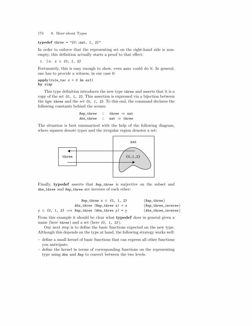
174 8. More about Types
typedef three = "{0::nat, 1, 2}"
In order to enforce that the representing set on the right-hand side is non-empty, this definition actually starts a proof to that effect:
1. ∃ x. x ∈ {0, 1, 2}
Fortunately, this is easy enough to show, even auto could do it. In general,one has to provide a witness, in our case 0:
apply(rule_tac x = 0 in exI)by simp
This type definition introduces the new type three and asserts that it is acopy of the set {0, 1, 2}. This assertion is expressed via a bijection betweenthe type three and the set {0, 1, 2}. To this end, the command declares thefollowing constants behind the scenes:
Rep_three :: three ⇒ nat
Abs_three :: nat ⇒ three
The situation is best summarized with the help of the following diagram,where squares denote types and the irregular region denotes a set:
three
nat
{0,1,2}
Finally, typedef asserts that Rep_three is surjective on the subset andAbs_three and Rep_three are inverses of each other:
Rep_three x ∈ {0, 1, 2} (Rep_three)Abs_three (Rep_three x) = x (Rep_three_inverse)
y ∈ {0, 1, 2} =⇒ Rep_three (Abs_three y) = y (Abs_three_inverse)
From this example it should be clear what typedef does in general given aname (here three) and a set (here {0, 1, 2}).
Our next step is to define the basic functions expected on the new type.Although this depends on the type at hand, the following strategy works well:
– define a small kernel of basic functions that can express all other functionsyou anticipate.
– define the kernel in terms of corresponding functions on the representingtype using Abs and Rep to convert between the two levels.
8.5 Introducing New Types 175
In our example it suffices to give the three elements of type three names:
definition A :: three where "A ≡ Abs_three 0"definition B :: three where "B ≡ Abs_three 1"definition C :: three where "C ≡ Abs_three 2"
So far, everything was easy. But it is clear that reasoning about three
will be hell if we have to go back to nat every time. Thus our aim must be toraise our level of abstraction by deriving enough theorems about type three
to characterize it completely. And those theorems should be phrased in termsof A, B and C, not Abs_three and Rep_three. Because of the simplicity of theexample, we merely need to prove that A, B and C are distinct and that theyexhaust the type.
In processing our typedef declaration, Isabelle proves several helpful lem-mas. The first two express injectivity of Rep_three and Abs_three :
(Rep_three x = Rep_three y) = (x = y) (Rep_three_inject)[[x ∈ {0, 1, 2}; y ∈ {0, 1, 2} ]]
=⇒ (Abs_three x = Abs_three y) = (x = y)(Abs_three_inject)
The following ones allow to replace some x::three by Abs_three(y::nat), andconversely y by Rep_three x :
[[y ∈ {0, 1, 2};∧x. y = Rep_three x =⇒ P ]] =⇒ P (Rep_three_cases)
(∧y. [[x = Abs_three y; y ∈ {0, 1, 2} ]] =⇒ P) =⇒ P (Abs_three_cases)
[[y ∈ {0, 1, 2};∧x. P (Rep_three x) ]] =⇒ P y (Rep_three_induct)
(∧y. y ∈ {0, 1, 2} =⇒ P (Abs_three y)) =⇒ P x (Abs_three_induct)
These theorems are proved for any type definition, with three replaced bythe name of the type in question.
Distinctness of A, B and C follows immediately if we expand their defini-tions and rewrite with the injectivity of Abs_three :
lemma "A 6= B ∧ B 6= A ∧ A 6= C ∧ C 6= A ∧ B 6= C ∧ C 6= B"by(simp add: Abs_three_inject A_def B_def C_def)
Of course we rely on the simplifier to solve goals like 0 6= 1.The fact that A, B and C exhaust type three is best phrased as a case
distinction theorem: if you want to prove P x (where x is of type three) itsuffices to prove P A, P B and P C :
lemma three_cases: " [[ P A; P B; P C ]] =⇒ P x"
Again this follows easily using the induction principle stemming from thetype definition:
apply(induct_tac x)
1.∧y. [[P A; P B; P C; y ∈ {0, 1, 2} ]] =⇒ P (Abs_three y)
Simplification leads to the disjunction y = 0 ∨ y = 1 ∨ y = 2 which auto
separates into three subgoals, each of which is easily solved by simplification:
176 8. More about Types
apply(auto simp add: A_def B_def C_def)done
This concludes the derivation of the characteristic theorems for type three.The attentive reader has realized long ago that the above lengthy defini-
tion can be collapsed into one line:
datatype better_three = A | B | C
In fact, the datatype command performs internally more or less the samederivations as we did, which gives you some idea what life would be likewithout datatype.
Although three could be defined in one line, we have chosen this exam-ple to demonstrate typedef because its simplicity makes the key conceptsparticularly easy to grasp. If you would like to see a non-trivial examplethat cannot be defined more directly, we recommend the definition of finitemultisets in the Library [4].
Let us conclude by summarizing the above procedure for defining a newtype. Given some abstract axiomatic description P of a type ty in terms ofa set of functions F , this involves three steps:
1. Find an appropriate type τ and subset A which has the desired propertiesP , and make a type definition based on this representation.
2. Define the required functions F on ty by lifting analogous functions onthe representation via Abs ty and Rep ty .
3. Prove that P holds for ty by lifting P from the representation.
You can now forget about the representation and work solely in terms of theabstract functions F and properties P .
9. Advanced Simplification and Induction
Although we have already learned a lot about simplification and induction,there are some advanced proof techniques that we have not covered yet andwhich are worth learning. The sections of this chapter are independent ofeach other and can be read in any order.
9.1 Simplification
This section describes features not covered until now. It also outlines thesimplification process itself, which can be helpful when the simplifier doesnot do what you expect of it.
9.1.1 Advanced Features
Congruence Rules. While simplifying the conclusion Q of P =⇒ Q , it islegal to use the assumption P . For =⇒ this policy is hardwired, but contextualinformation can also be made available for other operators. For example, xs= [] −→ xs @ xs = xs simplifies to True because we may use xs = [] whensimplifying xs @ xs = xs. The generation of contextual information duringsimplification is controlled by so-called congruence rules. This is the onefor −→:
[[P = P’; P’ =⇒ Q = Q’ ]] =⇒ (P −→ Q) = (P’ −→ Q’)
It should be read as follows: In order to simplify P −→ Q to P’ −→ Q’,simplify P to P’ and assume P’ when simplifying Q to Q’.
Here are some more examples. The congruence rules for bounded quanti-fiers supply contextual information about the bound variable:
[[A = B;∧x. x ∈ B =⇒ P x = Q x ]]
=⇒ (∀ x∈A. P x) = (∀ x∈B. Q x)
One congruence rule for conditional expressions supplies contextual informa-tion for simplifying the then and else cases:
[[b = c; c =⇒ x = u; ¬ c =⇒ y = v ]]=⇒ (if b then x else y) = (if c then u else v)
178 9. Advanced Simplification and Induction
An alternative congruence rule for conditional expressions actually preventssimplification of some arguments:
b = c =⇒ (if b then x else y) = (if c then x else y)
Only the first argument is simplified; the others remain unchanged. Thismakes simplification much faster and is faithful to the evaluation strategy inprogramming languages, which is why this is the default congruence rule forif. Analogous rules control the evaluation of case expressions.
You can declare your own congruence rules with the attribute cong , eitherglobally, in the usual manner,
declare theorem-name [cong]
or locally in a simp call by adding the modifier
cong: list of theorem names
The effect is reversed by cong del instead of cong.
!! The congruence rule conj_cong
[[P = P’; P’ =⇒ Q = Q’ ]] =⇒ (P ∧ Q) = (P’ ∧ Q’)
is occasionally useful but is not a default rule; you have to declare it explicitly.
Permutative Rewrite Rules. An equation is a permutative rewriterule if the left-hand side and right-hand side are the same up to renaming ofvariables. The most common permutative rule is commutativity: x + y = y +
x. Other examples include x - y - z = x - z - y in arithmetic and insert x
(insert y A) = insert y (insert x A) for sets. Such rules are problematicbecause once they apply, they can be used forever. The simplifier is aware ofthis danger and treats permutative rules by means of a special strategy, calledordered rewriting: a permutative rewrite rule is only applied if the termbecomes smaller with respect to a fixed lexicographic ordering on terms. Forexample, commutativity rewrites b + a to a + b, but then stops because a +
b is strictly smaller than b + a. Permutative rewrite rules can be turned intosimplification rules in the usual manner via the simp attribute; the simplifierrecognizes their special status automatically.
Permutative rewrite rules are most effective in the case of associative-commutative functions. (Associativity by itself is not permutative.) Whendealing with an AC-function f , keep the following points in mind:
– The associative law must always be oriented from left to right, namelyf (f (x , y), z ) = f (x , f (y , z )). The opposite orientation, if used with commu-tativity, can lead to nontermination.
– To complete your set of rewrite rules, you must add not just associativ-ity (A) and commutativity (C) but also a derived rule, left-commutativ-ity (LC): f (x , f (y , z )) = f (y , f (x , z )).
9.1 Simplification 179
Ordered rewriting with the combination of A, C, and LC sorts a term lexi-cographically:
f (f (b, c), a)A; f (b, f (c, a))
C; f (b, f (a, c))LC; f (a, f (b, c))
Note that ordered rewriting for + and * on numbers is rarely necessarybecause the built-in arithmetic prover often succeeds without such tricks.
9.1.2 How the Simplifier Works
Roughly speaking, the simplifier proceeds bottom-up: subterms are simplifiedfirst. A conditional equation is only applied if its condition can be proved,again by simplification. Below we explain some special features of the rewrit-ing process.
Higher-Order Patterns. So far we have pretended the simplifier can dealwith arbitrary rewrite rules. This is not quite true. For reasons of feasibility,the simplifier expects the left-hand side of each rule to be a so-called higher-order pattern [24]. This restricts where unknowns may occur. Higher-orderpatterns are terms in β-normal form. (This means there are no subtermsof the form (λx .M )(N ).) Each occurrence of an unknown is of the form?f x1 . . . xn , where the xi are distinct bound variables. Thus all ordinaryrewrite rules, where all unknowns are of base type, for example ?a + ?b + ?c
= ?a + (?b + ?c), are acceptable: if an unknown is of base type, it cannothave any arguments. Additionally, the rule (∀ x. ?P x ∧ ?Q x) = ((∀ x. ?P
x) ∧ (∀ x. ?Q x)) is also acceptable, in both directions: all arguments of theunknowns ?P and ?Q are distinct bound variables.
If the left-hand side is not a higher-order pattern, all is not lost. Thesimplifier will still try to apply the rule provided it matches directly: with-out much λ-calculus hocus pocus. For example, (?f ?x ∈ range ?f) = True
rewrites g a ∈ range g to True, but will fail to match g(h b) ∈ range(λx.
g(h x)). However, you can eliminate the offending subterms — those that arenot patterns — by adding new variables and conditions. In our example, weeliminate ?f ?x and obtain ?y = ?f ?x =⇒ (?y ∈ range ?f) = True, whichis fine as a conditional rewrite rule since conditions can be arbitrary terms.However, this trick is not a panacea because the newly introduced conditionsmay be hard to solve.
There is no restriction on the form of the right-hand sides. They may notcontain extraneous term or type variables, though.
The Preprocessor. When a theorem is declared a simplification rule, itneed not be a conditional equation already. The simplifier will turn it into aset of conditional equations automatically. For example, f x = g x ∧ h x =
k x becomes the two separate simplification rules f x = g x and h x = k x.In general, the input theorem is converted as follows:
180 9. Advanced Simplification and Induction
¬P 7→ P = False
P −→ Q 7→ P =⇒ Q
P ∧Q 7→ P , Q
∀x . P x 7→ P ?x
∀x ∈ A. P x 7→ ?x ∈ A =⇒ P ?x
if P then Q else R 7→ P =⇒ Q , ¬P =⇒ R
Once this conversion process is finished, all remaining non-equations P areturned into trivial equations P = True. For example, the formula
(p −→ t = u ∧ ¬ r) ∧ s
is converted into the three rules
p =⇒ t = u, p =⇒ r = False, s = True.
9.2 Advanced Induction Techniques
Now that we have learned about rules and logic, we take another look atthe finer points of induction. We consider two questions: what to do if theproposition to be proved is not directly amenable to induction (Sect. 9.2.1),and how to utilize (Sect. 9.2.2) and even derive (Sect. 9.2.3) new inductionschemas. We conclude with an extended example of induction (Sect. 9.2.4).
9.2.1 Massaging the Proposition
Often we have assumed that the theorem to be proved is already in a formthat is amenable to induction, but sometimes it isn’t. Here is an example.Since hd and last return the first and last element of a non-empty list, thislemma looks easy to prove:
lemma "xs 6= [] =⇒ hd(rev xs) = last xs"apply(induct_tac xs)
But induction produces the warning
Induction variable occurs also among premises!
and leads to the base case
1. xs 6= [] =⇒ hd (rev []) = last []A total of 2 subgoals...
Simplification reduces the base case to this:
1. xs 6= [] =⇒ hd [] = last []
9.2 Advanced Induction Techniques 181
We cannot prove this equality because we do not know what hd and last
return when applied to [].We should not have ignored the warning. Because the induction formula
is only the conclusion, induction does not affect the occurrence of xs in thepremises. Thus the case that should have been trivial becomes unprovable.Fortunately, the solution is easy:1
Pull all occurrences of the induction variable into the conclusion us-ing −→.
Thus we should state the lemma as an ordinary implication (−→), lettingrule_format (Sect. 5.15) convert the result to the usual =⇒ form:
lemma hd_rev [rule_format]: "xs 6= [] −→ hd(rev xs) = last xs"
This time, induction leaves us with a trivial base case:
1. [] 6= [] −→ hd (rev []) = last []A total of 2 subgoals...
And auto completes the proof.If there are multiple premises A1, . . . , An containing the induction vari-
able, you should turn the conclusion C into
A1 −→ · · ·An −→ C .
Additionally, you may also have to universally quantify some other variables,which can yield a fairly complex conclusion. However, rule_format can re-move any number of occurrences of ∀ and −→.
A second reason why your proposition may not be amenable to inductionis that you want to induct on a complex term, rather than a variable. Ingeneral, induction on a term t requires rephrasing the conclusion C as
∀y1 . . . yn . x = t −→ C . (9.1)
where y1 . . . yn are the free variables in t and x is a new variable. Now youcan perform induction on x . An example appears in Sect. 9.2.2 below.
The very same problem may occur in connection with rule induction.Remember that it requires a premise of the form (x1, . . . , xk ) ∈ R, where Ris some inductively defined set and the xi are variables. If instead we have apremise t ∈ R, where t is not just an n-tuple of variables, we replace it with(x1, . . . , xk ) ∈ R, and rephrase the conclusion C as
∀y1 . . . yn . (x1, . . . , xk ) = t −→ C .
For an example see Sect. 9.2.4 below.Of course, all premises that share free variables with t need to be pulled
into the conclusion as well, under the ∀ , again using −→ as shown above.
1 A similar heuristic applies to rule inductions; see Sect. 7.2.
182 9. Advanced Simplification and Induction
Readers who are puzzled by the form of statement (9.1) above shouldremember that the transformation is only performed to permit induction.Once induction has been applied, the statement can be transformed backinto something quite intuitive. For example, applying wellfounded inductionon x (w.r.t. ≺) to (9.1) and transforming the result a little leads to the goal∧
y . ∀z . t z ≺ t y −→ C z =⇒ C y
where y stands for y1 . . . yn and the dependence of t and C on the freevariables of t has been made explicit. Unfortunately, this induction schemacannot be expressed as a single theorem because it depends on the numberof free variables in t — the notation y is merely an informal device.
9.2.2 Beyond Structural and Recursion Induction
So far, inductive proofs were by structural induction for primitive recursivefunctions and recursion induction for total recursive functions. But some-times structural induction is awkward and there is no recursive function thatcould furnish a more appropriate induction schema. In such cases a general-purpose induction schema can be helpful. We show how to apply such induc-tion schemas by an example.
Structural induction on nat is usually known as mathematical induc-tion. There is also complete induction, where you prove P(n) under theassumption that P(m) holds for all m < n. In Isabelle, this is the theoremnat_less_induct :
(∧n. ∀ m<n. P m =⇒ P n) =⇒ P n
As an application, we prove a property of the following function:
axiomatization f :: "nat ⇒ nat"where f_ax: "f(f(n)) < f(Suc(n))" for n :: nat
!! We discourage the use of axioms because of the danger of inconsistencies. Ax-iom f_ax does not introduce an inconsistency because, for example, the identity
function satisfies it. Axioms can be useful in exploratory developments, say whenyou assume some well-known theorems so that you can quickly demonstrate somepoint about methodology. If your example turns into a substantial proof develop-ment, you should replace axioms by theorems.
The axiom for f implies n ≤ f n, which can be proved by induction on f n .Following the recipe outlined above, we have to phrase the proposition asfollows to allow induction:
lemma f_incr_lem: "∀ i. k = f i −→ i ≤ f i"
To perform induction on k using nat_less_induct, we use the same generalinduction method as for recursion induction (see Sect. 3.5.4):
apply(induct_tac k rule: nat_less_induct)
We get the following proof state:
9.2 Advanced Induction Techniques 183
1.∧n. ∀ m<n. ∀ i. m = f i −→ i ≤ f i =⇒ ∀ i. n = f i −→ i ≤ f i
After stripping the ∀ i, the proof continues with a case distinction on i. Thecase i = 0 is trivial and we focus on the other case:
apply(rule allI)apply(case_tac i)apply(simp)
1.∧n i nat.
[[∀ m<n. ∀ i. m = f i −→ i ≤ f i; i = Suc nat ]] =⇒ n = f i −→ i≤ f i
by(blast intro!: f_ax Suc_leI intro: le_less_trans)
If you find the last step puzzling, here are the two lemmas it employs:
m < n =⇒ Suc m ≤ n (Suc_leI)[[x ≤ y; y < z ]] =⇒ x < z (le_less_trans)
The proof goes like this (writing j instead of nat). Since i = Suc j it sufficesto show j < f (Suc j) , by Suc_leI . This is proved as follows. From f_ax wehave f (f j) < f (Suc j) (1) which implies f j ≤ f (f j) by the induc-tion hypothesis. Using (1) once more we obtain f j < f (Suc j) (2) by thetransitivity rule le_less_trans. Using the induction hypothesis once morewe obtain j ≤ f j which, together with (2) yields j < f (Suc j) (again byle_less_trans).
This last step shows both the power and the danger of automatic proofs.They will usually not tell you how the proof goes, because it can be hard totranslate the internal proof into a human-readable format. Automatic proofsare easy to write but hard to read and understand.
The desired result, i ≤ f i, follows from f_incr_lem :
lemmas f_incr = f_incr_lem[rule_format, OF refl]
The final refl gets rid of the premise ?k = f ?i. We could have included thisderivation in the original statement of the lemma:
lemma f_incr[rule_format, OF refl]: "∀ i. k = f i −→ i ≤ f i"
Exercise 9.2.1 From the axiom and lemma for f, show that f is the identityfunction.
Method induct_tac can be applied with any rule r whose conclusion is ofthe form ?P ?x1 . . .?xn , in which case the format is
apply(induct_tac y1 . . . yn rule: r)
where y1, . . . , yn are variables in the conclusion of the first subgoal.A further useful induction rule is length_induct, induction on the length
of a list
(∧xs. ∀ ys. length ys < length xs −→ P ys =⇒ P xs) =⇒ P xs
184 9. Advanced Simplification and Induction
which is a special case of measure_induct
(∧x. ∀ y. f y < f x −→ P y =⇒ P x) =⇒ P a
where f may be any function into type nat.
9.2.3 Derivation of New Induction Schemas
Induction schemas are ordinary theorems and you can derive new oneswhenever you wish. This section shows you how, using the example ofnat_less_induct. Assume we only have structural induction available for nat
and want to derive complete induction. We must generalize the statement asshown:
lemma induct_lem: "(∧n::nat. ∀ m<n. P m =⇒ P n) =⇒ ∀ m<n. P m"
apply(induct_tac n)
The base case is vacuously true. For the induction step (m < Suc n) we dis-tinguish two cases: case m < n is true by induction hypothesis and case m =
n follows from the assumption, again using the induction hypothesis:
apply(blast)by(blast elim: less_SucE)
The elimination rule less_SucE expresses the case distinction:
[[m < Suc n; m < n =⇒ P; m = n =⇒ P ]] =⇒ P
Now it is straightforward to derive the original version of nat_less_inductby manipulating the conclusion of the above lemma: instantiate n by Suc n
and m by n and remove the trivial condition n < Suc n. Fortunately, thishappens automatically when we add the lemma as a new premise to thedesired goal:
theorem nat_less_induct: "(∧n::nat. ∀ m<n. P m =⇒ P n) =⇒ P n"
by(insert induct_lem, blast)
HOL already provides the mother of all inductions, well-founded in-duction (see Sect. 6.4). For example theorem nat_less_induct is a specialcase of wf_induct where r is < on nat. The details can be found in theoryWellfounded_Recursion.
9.2.4 CTL Revisited
The purpose of this section is twofold: to demonstrate some of the inductionprinciples and heuristics discussed above and to show how inductive defi-nitions can simplify proofs. In Sect. 6.6.2 we gave a fairly involved proof ofthe correctness of a model checker for CTL. In particular the proof of theinfinity_lemma on the way to AF_lemma2 is not as simple as one might expect,
9.2 Advanced Induction Techniques 185
due to the SOME operator involved. Below we give a simpler proof of AF_lemma2based on an auxiliary inductive definition.
Let us call a (finite or infinite) path A-avoiding if it does not touch anynode in the set A. Then AF_lemma2 says that if no infinite path from some states is A -avoiding, then s ∈ lfp (af A). We prove this by inductively definingthe set Avoid s A of states reachable from s by a finite A -avoiding path:
inductive setAvoid :: "state ⇒ state set ⇒ state set"for s :: state and A :: "state set"
where"s ∈ Avoid s A"
| " [[ t ∈ Avoid s A; t /∈ A; (t,u) ∈ M ]] =⇒ u ∈ Avoid s A"
It is easy to see that for any infinite A -avoiding path f with f 0 ∈ Avoid
s A there is an infinite A -avoiding path starting with s because (by definitionof Avoid) there is a finite A -avoiding path from s to f 0. The proof is byinduction on f 0 ∈ Avoid s A. However, this requires the following reformu-lation, as explained in Sect. 9.2.1 above; the rule_format directive undoes thereformulation after the proof.
lemma ex_infinite_path[rule_format]:"t ∈ Avoid s A =⇒∀ f∈Paths t. (∀ i. f i /∈ A) −→ (∃ p∈Paths s. ∀ i. p i /∈ A)"
apply(erule Avoid.induct)apply(blast)
apply(clarify)apply(drule_tac x = "λi. case i of 0 ⇒ t | Suc i ⇒ f i" in bspec)apply(simp_all add: Paths_def split: nat.split)done
The base case (t = s) is trivial and proved by blast. In the induction step,we have an infinite A -avoiding path f starting from u, a successor of t. Nowwe simply instantiate the ∀ f∈Paths t in the induction hypothesis by thepath starting with t and continuing with f. That is what the above λ-termexpresses. Simplification shows that this is a path starting with t and thatthe instantiated induction hypothesis implies the conclusion.
Now we come to the key lemma. Assuming that no infinite A -avoidingpath starts from s, we want to show s ∈ lfp (af A). For the inductive proofthis must be generalized to the statement that every point t “between” s
and A, in other words all of Avoid s A, is contained in lfp (af A) :
lemma Avoid_in_lfp[rule_format(no_asm)]:"∀ p∈Paths s. ∃ i. p i ∈ A =⇒ t ∈ Avoid s A −→ t ∈ lfp(af A)"
The proof is by induction on the “distance” between t and A. Remember thatlfp (af A) = A ∪ M−1 ‘‘ lfp (af A). If t is already in A, then t ∈ lfp (af
A) is trivial. If t is not in A but all successors are in lfp (af A) (inductionhypothesis), then t ∈ lfp (af A) is again trivial.
The formal counterpart of this proof sketch is a well-founded inductionon M restricted to Avoid s A - A, roughly speaking:
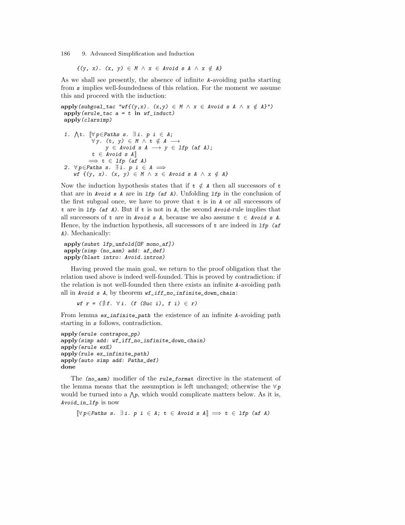
186 9. Advanced Simplification and Induction
{(y, x). (x, y) ∈ M ∧ x ∈ Avoid s A ∧ x /∈ A}
As we shall see presently, the absence of infinite A -avoiding paths startingfrom s implies well-foundedness of this relation. For the moment we assumethis and proceed with the induction:
apply(subgoal_tac "wf{(y,x). (x,y) ∈ M ∧ x ∈ Avoid s A ∧ x /∈ A}")apply(erule_tac a = t in wf_induct)apply(clarsimp)
1.∧t. [[∀ p∈Paths s. ∃ i. p i ∈ A;
∀ y. (t, y) ∈ M ∧ t /∈ A −→y ∈ Avoid s A −→ y ∈ lfp (af A);
t ∈ Avoid s A ]]=⇒ t ∈ lfp (af A)
2. ∀ p∈Paths s. ∃ i. p i ∈ A =⇒wf {(y, x). (x, y) ∈ M ∧ x ∈ Avoid s A ∧ x /∈ A}
Now the induction hypothesis states that if t /∈ A then all successors of t
that are in Avoid s A are in lfp (af A). Unfolding lfp in the conclusion ofthe first subgoal once, we have to prove that t is in A or all successors oft are in lfp (af A). But if t is not in A, the second Avoid -rule implies thatall successors of t are in Avoid s A, because we also assume t ∈ Avoid s A.Hence, by the induction hypothesis, all successors of t are indeed in lfp (af
A). Mechanically:
apply(subst lfp_unfold[OF mono_af])apply(simp (no_asm) add: af_def)apply(blast intro: Avoid.intros)
Having proved the main goal, we return to the proof obligation that therelation used above is indeed well-founded. This is proved by contradiction: ifthe relation is not well-founded then there exists an infinite A -avoiding pathall in Avoid s A, by theorem wf_iff_no_infinite_down_chain :
wf r = (@ f. ∀ i. (f (Suc i), f i) ∈ r)
From lemma ex_infinite_path the existence of an infinite A -avoiding pathstarting in s follows, contradiction.
apply(erule contrapos_pp)apply(simp add: wf_iff_no_infinite_down_chain)apply(erule exE)apply(rule ex_infinite_path)apply(auto simp add: Paths_def)done
The (no_asm) modifier of the rule_format directive in the statement ofthe lemma means that the assumption is left unchanged; otherwise the ∀ pwould be turned into a
∧p, which would complicate matters below. As it is,
Avoid_in_lfp is now
[[∀ p∈Paths s. ∃ i. p i ∈ A; t ∈ Avoid s A ]] =⇒ t ∈ lfp (af A)

9.2 Advanced Induction Techniques 187
The main theorem is simply the corollary where t = s, when the assumptiont ∈ Avoid s A is trivially true by the first Avoid -rule. Isabelle confirms this:
theorem AF_lemma2: "{s. ∀ p ∈ Paths s. ∃ i. p i ∈ A} ⊆ lfp(af A)"by(auto elim: Avoid_in_lfp intro: Avoid.intros)

10. Case Study: Verifying a Security Protocol
Communications security is an ancient art. Julius Caesar is said to haveencrypted his messages, shifting each letter three places along the alphabet.Mary Queen of Scots was convicted of treason after a cipher used in herletters was broken. Today’s postal system incorporates security features. Theenvelope provides a degree of secrecy. The signature provides authenticity(proof of origin), as do departmental stamps and letterheads.
Networks are vulnerable: messages pass through many computers, any ofwhich might be controlled by an adversary, who thus can capture or redirectmessages. People who wish to communicate securely over such a network canuse cryptography, but if they are to understand each other, they need tofollow a protocol : a pre-arranged sequence of message formats.
Protocols can be attacked in many ways, even if encryption is unbreak-able. A splicing attack involves an adversary’s sending a message composedof parts of several old messages. This fake message may have the correct for-mat, fooling an honest party. The adversary might be able to masquerade assomebody else, or he might obtain a secret key.
Nonces help prevent splicing attacks. A typical nonce is a 20-byte randomnumber. Each message that requires a reply incorporates a nonce. The replymust include a copy of that nonce, to prove that it is not a replay of a pastmessage. The nonce in the reply must be cryptographically protected, sinceotherwise an adversary could easily replace it by a different one. You shouldbe starting to see that protocol design is tricky!
Researchers are developing methods for proving the correctness of securityprotocols. The Needham-Schroeder public-key protocol [23] has become astandard test case. Proposed in 1978, it was found to be defective nearly twodecades later [19]. This toy protocol will be useful in demonstrating how toverify protocols using Isabelle.
10.1 The Needham-Schroeder Public-Key Protocol
This protocol uses public-key cryptography. Each person has a private key,known only to himself, and a public key, known to everybody. If Alice wantsto send Bob a secret message, she encrypts it using Bob’s public key (which
190 10. Case Study: Verifying a Security Protocol
everybody knows), and sends it to Bob. Only Bob has the matching privatekey, which is needed in order to decrypt Alice’s message.
The core of the Needham-Schroeder protocol consists of three messages:
1. A→ B : {|Na,A|}Kb
2. B → A : {|Na,Nb|}Ka
3. A→ B : {|Nb|}Kb
First, let’s understand the notation. In the first message, Alice sends Bob amessage consisting of a nonce generated by Alice (Na) paired with Alice’sname (A) and encrypted using Bob’s public key (Kb). In the second message,Bob sends Alice a message consisting of Na paired with a nonce generatedby Bob (Nb), encrypted using Alice’s public key (Ka). In the last message,Alice returns Nb to Bob, encrypted using his public key.
When Alice receives Message 2, she knows that Bob has acted on hermessage, since only he could have decrypted {|Na,A|}Kb and extracted Na.That is precisely what nonces are for. Similarly, message 3 assures Bob thatAlice is active. But the protocol was widely believed [7] to satisfy a furtherproperty: that Na and Nb were secrets shared by Alice and Bob. (Manyprotocols generate such shared secrets, which can be used to lessen the re-liance on slow public-key operations.) Lowe found this claim to be false: ifAlice runs the protocol with someone untrustworthy (Charlie say), then hecan start a new run with another agent (Bob say). Charlie uses Alice as anoracle, masquerading as Alice to Bob [19].
1. A→ C : {|Na,A|}Kc 1′. C → B : {|Na,A|}Kb
2. B → A : {|Na,Nb|}Ka
3. A→ C : {|Nb|}Kc 3′. C → B : {|Nb|}Kb
In messages 1 and 3, Charlie removes the encryption using his private keyand re-encrypts Alice’s messages using Bob’s public key. Bob is left thinkinghe has run the protocol with Alice, which was not Alice’s intention, and Bobis unaware that the “secret” nonces are known to Charlie. This is a typicalman-in-the-middle attack launched by an insider.
Whether this counts as an attack has been disputed. In protocols ofthis type, we normally assume that the other party is honest. To be hon-est means to obey the protocol rules, so Alice’s running the protocol withCharlie does not make her dishonest, just careless. After Lowe’s attack, Alicehas no grounds for complaint: this protocol does not have to guarantee any-thing if you run it with a bad person. Bob does have grounds for complaint,however: the protocol tells him that he is communicating with Alice (who ishonest) but it does not guarantee secrecy of the nonces.
Lowe also suggested a correction, namely to include Bob’s name in mes-sage 2:
10.2 Agents and Messages 191
1. A→ B : {|Na,A|}Kb
2. B → A : {|Na,Nb,B |}Ka
3. A→ B : {|Nb|}Kb
If Charlie tries the same attack, Alice will receive the message {|Na,Nb,B |}Ka
when she was expecting to receive {|Na,Nb,C |}Ka . She will abandon the run,and eventually so will Bob. Below, we shall look at parts of this protocol’scorrectness proof.
In ground-breaking work, Lowe [19] showed how such attacks could befound automatically using a model checker. An alternative, which we shallexamine below, is to prove protocols correct. Proofs can be done under morerealistic assumptions because our model does not have to be finite. The strat-egy is to formalize the operational semantics of the system and to provesecurity properties using rule induction.
10.2 Agents and Messages
All protocol specifications refer to a syntactic theory of messages. Datatypeagent introduces the constant Server (a trusted central machine, needed forsome protocols), an infinite population of friendly agents, and the Spy :
datatype agent = Server | Friend nat | Spy
Keys are just natural numbers. Function invKey maps a public key to thematching private key, and vice versa:
type synonym key = natconsts invKey :: "key ⇒ key"
Datatype msg introduces the message forms, which include agent names,nonces, keys, compound messages, and encryptions.
datatypemsg = Agent agent
| Nonce nat| Key key| MPair msg msg| Crypt key msg
The notation {|X1, . . .Xn−1,Xn |} abbreviates MPairX1 . . . (MPairXn−1 Xn).Since datatype constructors are injective, we have the theorem
Crypt K X = Crypt K’ X’ =⇒ K = K’ ∧ X = X’
A ciphertext can be decrypted using only one key and can yield only oneplaintext. In the real world, decryption with the wrong key succeeds butyields garbage. Our model of encryption is realistic if encryption adds someredundancy to the plaintext, such as a checksum, so that garbage can bedetected.
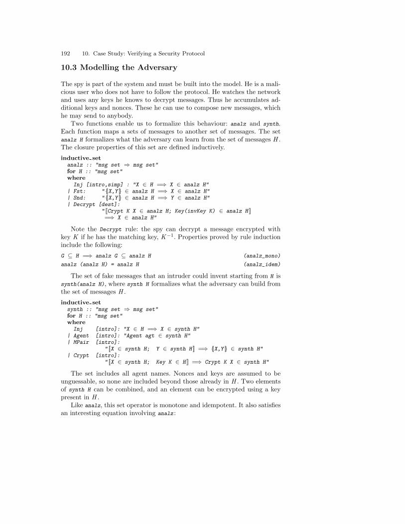
192 10. Case Study: Verifying a Security Protocol
10.3 Modelling the Adversary
The spy is part of the system and must be built into the model. He is a mali-cious user who does not have to follow the protocol. He watches the networkand uses any keys he knows to decrypt messages. Thus he accumulates ad-ditional keys and nonces. These he can use to compose new messages, whichhe may send to anybody.
Two functions enable us to formalize this behaviour: analz and synth.Each function maps a sets of messages to another set of messages. The setanalz H formalizes what the adversary can learn from the set of messages H .The closure properties of this set are defined inductively.
inductive setanalz :: "msg set ⇒ msg set"for H :: "msg set"where
Inj [intro,simp] : "X ∈ H =⇒ X ∈ analz H"| Fst: "{|X,Y |} ∈ analz H =⇒ X ∈ analz H"| Snd: "{|X,Y |} ∈ analz H =⇒ Y ∈ analz H"| Decrypt [dest]:
" [[Crypt K X ∈ analz H; Key(invKey K) ∈ analz H ]]=⇒ X ∈ analz H"
Note the Decrypt rule: the spy can decrypt a message encrypted withkey K if he has the matching key, K−1. Properties proved by rule inductioninclude the following:
G ⊆ H =⇒ analz G ⊆ analz H (analz_mono)
analz (analz H) = analz H (analz_idem)
The set of fake messages that an intruder could invent starting from H issynth(analz H), where synth H formalizes what the adversary can build fromthe set of messages H .
inductive setsynth :: "msg set ⇒ msg set"for H :: "msg set"where
Inj [intro]: "X ∈ H =⇒ X ∈ synth H"| Agent [intro]: "Agent agt ∈ synth H"| MPair [intro]:
" [[X ∈ synth H; Y ∈ synth H ]] =⇒ {|X,Y |} ∈ synth H"| Crypt [intro]:
" [[X ∈ synth H; Key K ∈ H ]] =⇒ Crypt K X ∈ synth H"
The set includes all agent names. Nonces and keys are assumed to beunguessable, so none are included beyond those already in H . Two elementsof synth H can be combined, and an element can be encrypted using a keypresent in H .
Like analz, this set operator is monotone and idempotent. It also satisfiesan interesting equation involving analz :
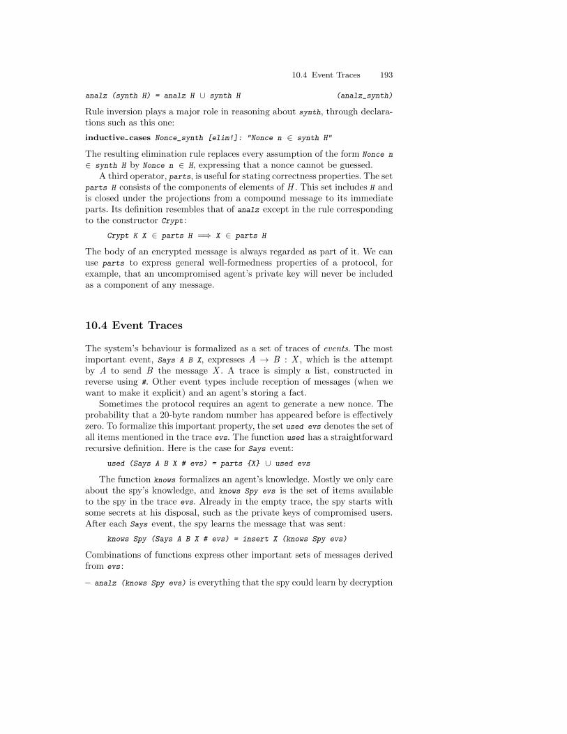
10.4 Event Traces 193
analz (synth H) = analz H ∪ synth H (analz_synth)
Rule inversion plays a major role in reasoning about synth, through declara-tions such as this one:
inductive cases Nonce_synth [elim!]: "Nonce n ∈ synth H"
The resulting elimination rule replaces every assumption of the form Nonce n
∈ synth H by Nonce n ∈ H, expressing that a nonce cannot be guessed.A third operator, parts, is useful for stating correctness properties. The set
parts H consists of the components of elements of H . This set includes H andis closed under the projections from a compound message to its immediateparts. Its definition resembles that of analz except in the rule correspondingto the constructor Crypt :
Crypt K X ∈ parts H =⇒ X ∈ parts H
The body of an encrypted message is always regarded as part of it. We canuse parts to express general well-formedness properties of a protocol, forexample, that an uncompromised agent’s private key will never be includedas a component of any message.
10.4 Event Traces
The system’s behaviour is formalized as a set of traces of events. The mostimportant event, Says A B X, expresses A → B : X , which is the attemptby A to send B the message X . A trace is simply a list, constructed inreverse using #. Other event types include reception of messages (when wewant to make it explicit) and an agent’s storing a fact.
Sometimes the protocol requires an agent to generate a new nonce. Theprobability that a 20-byte random number has appeared before is effectivelyzero. To formalize this important property, the set used evs denotes the set ofall items mentioned in the trace evs. The function used has a straightforwardrecursive definition. Here is the case for Says event:
used (Says A B X # evs) = parts {X} ∪ used evs
The function knows formalizes an agent’s knowledge. Mostly we only careabout the spy’s knowledge, and knows Spy evs is the set of items availableto the spy in the trace evs. Already in the empty trace, the spy starts withsome secrets at his disposal, such as the private keys of compromised users.After each Says event, the spy learns the message that was sent:
knows Spy (Says A B X # evs) = insert X (knows Spy evs)
Combinations of functions express other important sets of messages derivedfrom evs :
– analz (knows Spy evs) is everything that the spy could learn by decryption
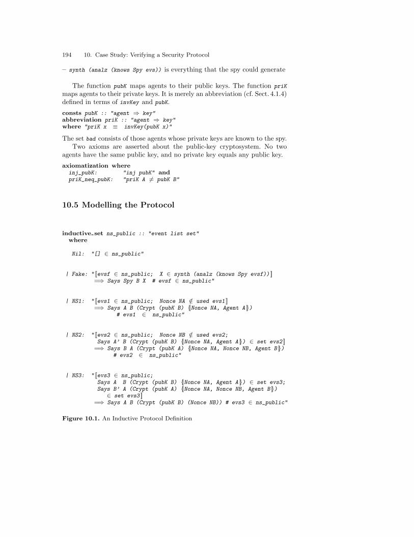
194 10. Case Study: Verifying a Security Protocol
– synth (analz (knows Spy evs)) is everything that the spy could generate
The function pubK maps agents to their public keys. The function priK
maps agents to their private keys. It is merely an abbreviation (cf. Sect. 4.1.4)defined in terms of invKey and pubK.
consts pubK :: "agent ⇒ key"abbreviation priK :: "agent ⇒ key"where "priK x ≡ invKey(pubK x)"
The set bad consists of those agents whose private keys are known to the spy.Two axioms are asserted about the public-key cryptosystem. No two
agents have the same public key, and no private key equals any public key.
axiomatization whereinj_pubK: "inj pubK" andpriK_neq_pubK: "priK A 6= pubK B"
10.5 Modelling the Protocol
inductive set ns_public :: "event list set"where
Nil: "[] ∈ ns_public"
| Fake: " [[evsf ∈ ns_public; X ∈ synth (analz (knows Spy evsf)) ]]=⇒ Says Spy B X # evsf ∈ ns_public"
| NS1: " [[evs1 ∈ ns_public; Nonce NA /∈ used evs1 ]]=⇒ Says A B (Crypt (pubK B) {|Nonce NA, Agent A |})
# evs1 ∈ ns_public"
| NS2: " [[evs2 ∈ ns_public; Nonce NB /∈ used evs2;Says A’ B (Crypt (pubK B) {|Nonce NA, Agent A |}) ∈ set evs2 ]]
=⇒ Says B A (Crypt (pubK A) {|Nonce NA, Nonce NB, Agent B |})# evs2 ∈ ns_public"
| NS3: " [[evs3 ∈ ns_public;Says A B (Crypt (pubK B) {|Nonce NA, Agent A |}) ∈ set evs3;Says B’ A (Crypt (pubK A) {|Nonce NA, Nonce NB, Agent B |})∈ set evs3 ]]
=⇒ Says A B (Crypt (pubK B) (Nonce NB)) # evs3 ∈ ns_public"
Figure 10.1. An Inductive Protocol Definition
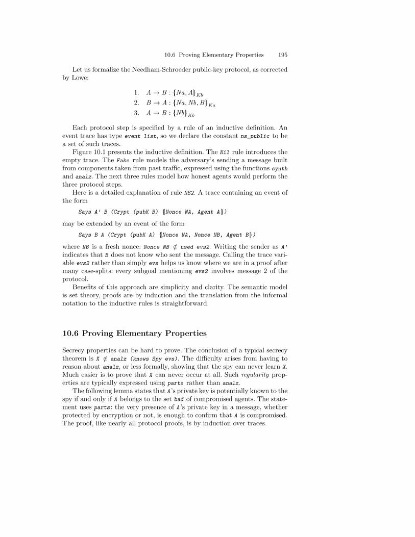
10.6 Proving Elementary Properties 195
Let us formalize the Needham-Schroeder public-key protocol, as correctedby Lowe:
1. A→ B : {|Na,A|}Kb
2. B → A : {|Na,Nb,B |}Ka
3. A→ B : {|Nb|}Kb
Each protocol step is specified by a rule of an inductive definition. Anevent trace has type event list, so we declare the constant ns_public to bea set of such traces.
Figure 10.1 presents the inductive definition. The Nil rule introduces theempty trace. The Fake rule models the adversary’s sending a message builtfrom components taken from past traffic, expressed using the functions synth
and analz. The next three rules model how honest agents would perform thethree protocol steps.
Here is a detailed explanation of rule NS2. A trace containing an event ofthe form
Says A’ B (Crypt (pubK B) {|Nonce NA, Agent A |})
may be extended by an event of the form
Says B A (Crypt (pubK A) {|Nonce NA, Nonce NB, Agent B |})
where NB is a fresh nonce: Nonce NB /∈ used evs2. Writing the sender as A’
indicates that B does not know who sent the message. Calling the trace vari-able evs2 rather than simply evs helps us know where we are in a proof aftermany case-splits: every subgoal mentioning evs2 involves message 2 of theprotocol.
Benefits of this approach are simplicity and clarity. The semantic modelis set theory, proofs are by induction and the translation from the informalnotation to the inductive rules is straightforward.
10.6 Proving Elementary Properties
Secrecy properties can be hard to prove. The conclusion of a typical secrecytheorem is X /∈ analz (knows Spy evs). The difficulty arises from having toreason about analz, or less formally, showing that the spy can never learn X.Much easier is to prove that X can never occur at all. Such regularity prop-erties are typically expressed using parts rather than analz.
The following lemma states that A ’s private key is potentially known to thespy if and only if A belongs to the set bad of compromised agents. The state-ment uses parts : the very presence of A ’s private key in a message, whetherprotected by encryption or not, is enough to confirm that A is compromised.The proof, like nearly all protocol proofs, is by induction over traces.
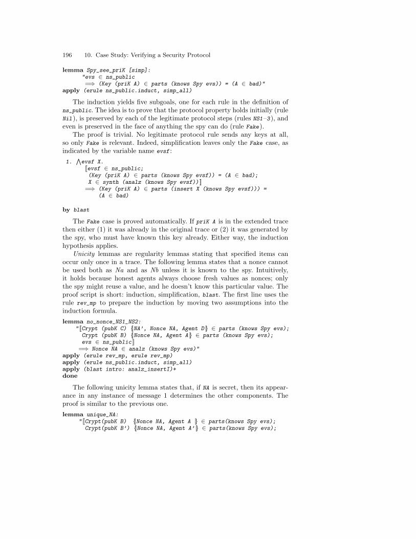
196 10. Case Study: Verifying a Security Protocol
lemma Spy_see_priK [simp]:"evs ∈ ns_public=⇒ (Key (priK A) ∈ parts (knows Spy evs)) = (A ∈ bad)"
apply (erule ns_public.induct, simp_all)
The induction yields five subgoals, one for each rule in the definition ofns_public. The idea is to prove that the protocol property holds initially (ruleNil), is preserved by each of the legitimate protocol steps (rules NS1–3), andeven is preserved in the face of anything the spy can do (rule Fake).
The proof is trivial. No legitimate protocol rule sends any keys at all,so only Fake is relevant. Indeed, simplification leaves only the Fake case, asindicated by the variable name evsf :
1.∧evsf X.
[[evsf ∈ ns_public;(Key (priK A) ∈ parts (knows Spy evsf)) = (A ∈ bad);X ∈ synth (analz (knows Spy evsf)) ]]
=⇒ (Key (priK A) ∈ parts (insert X (knows Spy evsf))) =(A ∈ bad)
by blast
The Fake case is proved automatically. If priK A is in the extended tracethen either (1) it was already in the original trace or (2) it was generated bythe spy, who must have known this key already. Either way, the inductionhypothesis applies.
Unicity lemmas are regularity lemmas stating that specified items canoccur only once in a trace. The following lemma states that a nonce cannotbe used both as Na and as Nb unless it is known to the spy. Intuitively,it holds because honest agents always choose fresh values as nonces; onlythe spy might reuse a value, and he doesn’t know this particular value. Theproof script is short: induction, simplification, blast. The first line uses therule rev_mp to prepare the induction by moving two assumptions into theinduction formula.
lemma no_nonce_NS1_NS2:" [[Crypt (pubK C) {|NA’, Nonce NA, Agent D |} ∈ parts (knows Spy evs);Crypt (pubK B) {|Nonce NA, Agent A |} ∈ parts (knows Spy evs);evs ∈ ns_public ]]
=⇒ Nonce NA ∈ analz (knows Spy evs)"apply (erule rev_mp, erule rev_mp)apply (erule ns_public.induct, simp_all)apply (blast intro: analz_insertI)+done
The following unicity lemma states that, if NA is secret, then its appear-ance in any instance of message 1 determines the other components. Theproof is similar to the previous one.
lemma unique_NA:" [[Crypt(pubK B) {|Nonce NA, Agent A |} ∈ parts(knows Spy evs);Crypt(pubK B’) {|Nonce NA, Agent A’ |} ∈ parts(knows Spy evs);
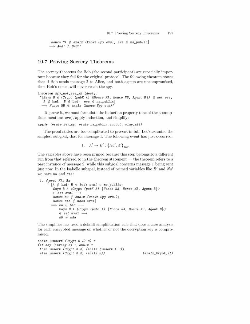
10.7 Proving Secrecy Theorems 197
Nonce NA /∈ analz (knows Spy evs); evs ∈ ns_public ]]=⇒ A=A’ ∧ B=B’"
10.7 Proving Secrecy Theorems
The secrecy theorems for Bob (the second participant) are especially impor-tant because they fail for the original protocol. The following theorem statesthat if Bob sends message 2 to Alice, and both agents are uncompromised,then Bob’s nonce will never reach the spy.
theorem Spy_not_see_NB [dest]:" [[Says B A (Crypt (pubK A) {|Nonce NA, Nonce NB, Agent B |}) ∈ set evs;A /∈ bad; B /∈ bad; evs ∈ ns_public ]]
=⇒ Nonce NB /∈ analz (knows Spy evs)"
To prove it, we must formulate the induction properly (one of the assump-tions mentions evs), apply induction, and simplify:
apply (erule rev_mp, erule ns_public.induct, simp_all)
The proof states are too complicated to present in full. Let’s examine thesimplest subgoal, that for message 1. The following event has just occurred:
1. A′ → B ′ : {|Na ′,A′|}Kb′
The variables above have been primed because this step belongs to a differentrun from that referred to in the theorem statement — the theorem refers to apast instance of message 2, while this subgoal concerns message 1 being sentjust now. In the Isabelle subgoal, instead of primed variables like B ′ and Na ′
we have Ba and NAa :
1.∧evs1 NAa Ba.
[[A /∈ bad; B /∈ bad; evs1 ∈ ns_public;Says B A (Crypt (pubK A) {|Nonce NA, Nonce NB, Agent B |})∈ set evs1 −→Nonce NB /∈ analz (knows Spy evs1);Nonce NAa /∈ used evs1 ]]
=⇒ Ba ∈ bad −→Says B A (Crypt (pubK A) {|Nonce NA, Nonce NB, Agent B |})∈ set evs1 −→NB 6= NAa
The simplifier has used a default simplification rule that does a case analysisfor each encrypted message on whether or not the decryption key is compro-mised.
analz (insert (Crypt K X) H) =(if Key (invKey K) ∈ analz Hthen insert (Crypt K X) (analz (insert X H))else insert (Crypt K X) (analz H)) (analz_Crypt_if)
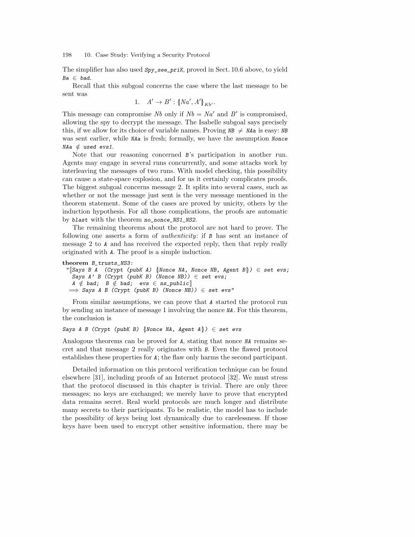
198 10. Case Study: Verifying a Security Protocol
The simplifier has also used Spy_see_priK, proved in Sect. 10.6 above, to yieldBa ∈ bad.
Recall that this subgoal concerns the case where the last message to besent was
1. A′ → B ′ : {|Na ′,A′|}Kb′ .
This message can compromise Nb only if Nb = Na ′ and B ′ is compromised,allowing the spy to decrypt the message. The Isabelle subgoal says preciselythis, if we allow for its choice of variable names. Proving NB 6= NAa is easy: NBwas sent earlier, while NAa is fresh; formally, we have the assumption Nonce
NAa /∈ used evs1.Note that our reasoning concerned B ’s participation in another run.
Agents may engage in several runs concurrently, and some attacks work byinterleaving the messages of two runs. With model checking, this possibilitycan cause a state-space explosion, and for us it certainly complicates proofs.The biggest subgoal concerns message 2. It splits into several cases, such aswhether or not the message just sent is the very message mentioned in thetheorem statement. Some of the cases are proved by unicity, others by theinduction hypothesis. For all those complications, the proofs are automaticby blast with the theorem no_nonce_NS1_NS2.
The remaining theorems about the protocol are not hard to prove. Thefollowing one asserts a form of authenticity : if B has sent an instance ofmessage 2 to A and has received the expected reply, then that reply reallyoriginated with A. The proof is a simple induction.
theorem B_trusts_NS3:" [[Says B A (Crypt (pubK A) {|Nonce NA, Nonce NB, Agent B |}) ∈ set evs;
Says A’ B (Crypt (pubK B) (Nonce NB)) ∈ set evs;A /∈ bad; B /∈ bad; evs ∈ ns_public ]]
=⇒ Says A B (Crypt (pubK B) (Nonce NB)) ∈ set evs"
From similar assumptions, we can prove that A started the protocol runby sending an instance of message 1 involving the nonce NA . For this theorem,the conclusion is
Says A B (Crypt (pubK B) {|Nonce NA, Agent A |}) ∈ set evs
Analogous theorems can be proved for A, stating that nonce NA remains se-cret and that message 2 really originates with B. Even the flawed protocolestablishes these properties for A ; the flaw only harms the second participant.
Detailed information on this protocol verification technique can be foundelsewhere [31], including proofs of an Internet protocol [32]. We must stressthat the protocol discussed in this chapter is trivial. There are only threemessages; no keys are exchanged; we merely have to prove that encrypteddata remains secret. Real world protocols are much longer and distributemany secrets to their participants. To be realistic, the model has to includethe possibility of keys being lost dynamically due to carelessness. If thosekeys have been used to encrypt other sensitive information, there may be

199
cascading losses. We may still be able to establish a bound on the losses andto prove that other protocol runs function correctly [33]. Proofs of real-worldprotocols follow the strategy illustrated above, but the subgoals can be muchbigger and there are more of them.

200

201
You know my methods. Apply them!
Sherlock Holmes

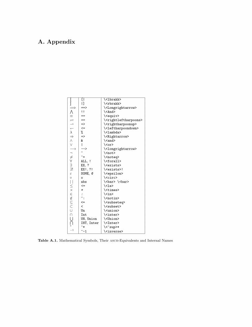
A. Appendix
[[ [| \<lbrakk>]] |] \<rbrakk>=⇒ ==> \<Longrightarrow>∧
!! \<And>≡ == \<equiv> == \<rightleftharpoons>⇀ => \<rightharpoonup>↽ <= \<leftharpoondown>λ % \<lambda>⇒ => \<Rightarrow>∧ & \<and>∨ | \<or>−→ --> \<longrightarrow>¬ ~ \<not>6= ~= \<noteq>∀ ALL, ! \<forall>∃ EX, ? \<exists>∃! EX!, ?! \<exists>!ε SOME, @ \<epsilon>◦ o \<circ>| | abs \<bar> \<bar>≤ <= \<le>× * \<times>∈ : \<in>/∈ ~: \<notin>⊆ <= \<subseteq>⊂ < \<subset>∪ Un \<union>∩ Int \<inter>⋃
UN, Union \<Union>⋂INT, Inter \<Inter>
∗ ^* \<^sup>*−1 ^-1 \<inverse>
Table A.1. Mathematical Symbols, Their ascii-Equivalents and Internal Names
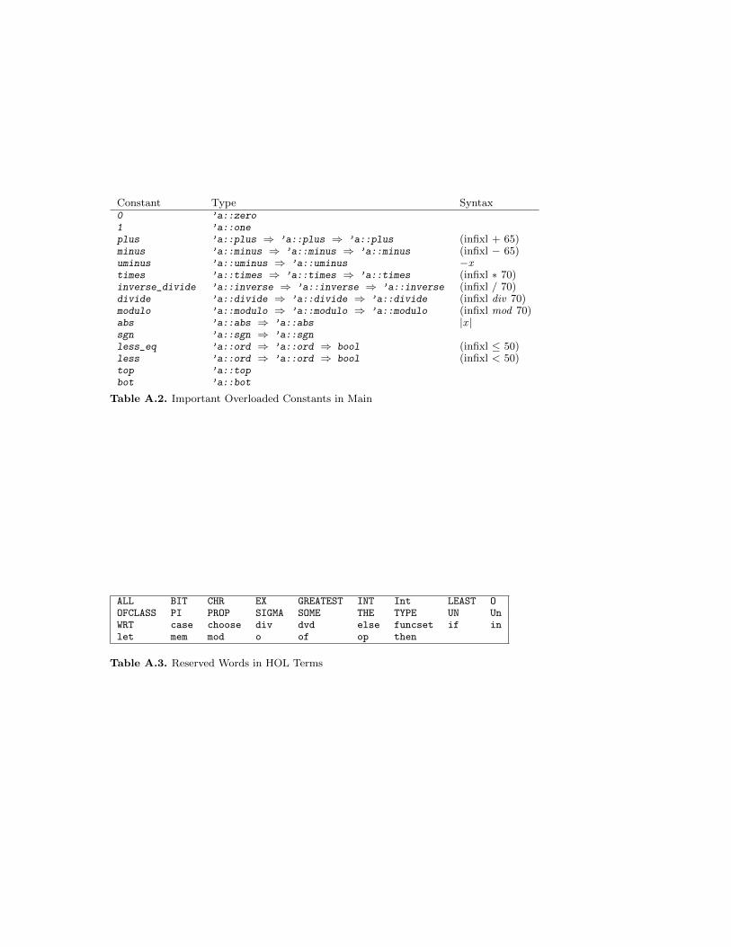
Constant Type Syntax0 ’a::zero1 ’a::oneplus ’a::plus ⇒ ’a::plus ⇒ ’a::plus (infixl + 65)minus ’a::minus ⇒ ’a::minus ⇒ ’a::minus (infixl − 65)uminus ’a::uminus ⇒ ’a::uminus −xtimes ’a::times ⇒ ’a::times ⇒ ’a::times (infixl ∗ 70)inverse_divide ’a::inverse ⇒ ’a::inverse ⇒ ’a::inverse (infixl / 70)divide ’a::divide ⇒ ’a::divide ⇒ ’a::divide (infixl div 70)modulo ’a::modulo ⇒ ’a::modulo ⇒ ’a::modulo (infixl mod 70)abs ’a::abs ⇒ ’a::abs |x |sgn ’a::sgn ⇒ ’a::sgnless_eq ’a::ord ⇒ ’a::ord ⇒ bool (infixl ≤ 50)less ’a::ord ⇒ ’a::ord ⇒ bool (infixl < 50)top ’a::topbot ’a::bot
Table A.2. Important Overloaded Constants in Main
ALL BIT CHR EX GREATEST INT Int LEAST OOFCLASS PI PROP SIGMA SOME THE TYPE UN UnWRT case choose div dvd else funcset if inlet mem mod o of op then
Table A.3. Reserved Words in HOL Terms
Bibliography
[1] David Aspinall. Proof General. http://proofgeneral.inf.ed.ac.uk/.[2] David Aspinall. Proof General: A generic tool for proof development.
In Tools and Algorithms for the Construction and Analysis of Systems(TACAS), volume 1785 of Lecture Notes in Computer Science, pages38–42. Springer-Verlag, 2000.
[3] Franz Baader and Tobias Nipkow. Term Rewriting and All That. Cam-bridge University Press, 1998.
[4] Gertrud Bauer, Tobias Nipkow, David von Oheimb, Lawrence C Paulson,Thomas M Rasmussen, Christophe Tabacznyj, and Markus Wenzel. Thesupplemental Isabelle/HOL library. Part of the Isabelle distribution,https://isabelle.in.tum.de/library/HOL/Library/document.pdf, 2002.
[5] Richard Bird. Introduction to Functional Programming using Haskell.Prentice-Hall, 1998.
[6] Lukas Bulwahn, Alexander Krauss, and Tobias Nipkow. Finding lexi-cographic orders for termination proofs in Isabelle/HOL. In K. Schnei-der and J. Brandt, editors, Theorem Proving in Higher Order Logics:TPHOLs 2007, volume 4732 of Lecture Notes in Computer Science,pages 38–53. Springer-Verlag, 2007.
[7] M. Burrows, M. Abadi, and R. M. Needham. A logic of authentication.Proceedings of the Royal Society of London, 426:233–271, 1989.
[8] Edmund Clarke, Orna Grumberg, and Doron Peled. Model Checking.MIT Press, 1999.
[9] Jacques Fleuriot and Lawrence C. Paulson. Mechanizing nonstandardreal analysis. LMS Journal of Computation and Mathematics, 3:140–190,2000. http://www.lms.ac.uk/jcm/3/lms1999-027/.
[10] Jean-Yves Girard. Proofs and Types. Cambridge University Press, 1989.Translated by Yves Lafont and Paul Taylor.
[11] M. J. C. Gordon and T. F. Melham, editors. Introduction to HOL:A Theorem Proving Environment for Higher Order Logic. CambridgeUniversity Press, 1993.
[12] Florian Haftmann. Haskell-style type classes with Isabelle/Isar. https://isabelle.in.tum.de/doc/classes.pdf.
[13] David Harel, Dexter Kozen, and Jerzy Tiuryn. Dynamic Logic. MITPress, 2000.
206 BIBLIOGRAPHY
[14] John E. Hopcroft and Jeffrey D. Ullman. Introduction to AutomataTheory, Languages, and Computation. Addison-Wesley, 1979.
[15] Paul Hudak. The Haskell School of Expression. Cambridge UniversityPress, 2000.
[16] Michael Huth and Mark Ryan. Logic in Computer Science. Modellingand reasoning about systems. Cambridge University Press, 2000.
[17] Donald E. Knuth. The Art of Computer Programming, Volume 3: Sort-ing and Searching. Addison-Wesley, 1975.
[18] Alexander Krauss. Defining Recursive Functions in Isabelle/HOL. https://isabelle.in.tum.de/doc/functions.pdf.
[19] Gavin Lowe. Breaking and fixing the Needham-Schroeder public-keyprotocol using CSP and FDR. In T. Margaria and B. Steffen, editors,Tools and Algorithms for the Construction and Analysis of Systems:second international workshop, TACAS ’96, LNCS 1055, pages 147–166.Springer, 1996.
[20] Robin Milner, Mads Tofte, and Robert Harper. The Definition of Stan-dard ML. MIT Press, 1990.
[21] Olaf Muller, Tobias Nipkow, David von Oheimb, and Oscar Slotosch.HOLCF = HOL + LCF. Journal of Functional Programming, 9:191–223, 1999.
[22] Wolfgang Naraschewski and Markus Wenzel. Object-oriented verifica-tion based on record subtyping in higher-order logic. In Jim Grundyand Malcom Newey, editors, Theorem Proving in Higher Order Log-ics: TPHOLs ’98, volume 1479 of Lecture Notes in Computer Science.Springer-Verlag, 1998.
[23] Roger M. Needham and Michael D. Schroeder. Using encryption forauthentication in large networks of computers. Communications of theACM, 21(12):993–999, December 1978.
[24] Tobias Nipkow. Functional unification of higher-order patterns. InM. Vardi, editor, Eighth Annual Symposium on Logic in Computer Sci-ence, pages 64–74. IEEE Computer Society Press, 1993.
[25] Tobias Nipkow. Structured Proofs in Isar/HOL. In H. Geuvers andF. Wiedijk, editors, Types for Proofs and Programs (TYPES 2002),volume 2646 of Lecture Notes in Computer Science, pages 259–278.Springer-Verlag, 2003.
[26] Tobias Nipkow, Lawrence C. Paulson, and Markus Wenzel. Isabelle’sLogics: HOL. https://isabelle.in.tum.de/doc/logics-HOL.pdf.
[27] Lawrence C. Paulson. The Old Isabelle Reference Manual. https://isabelle.in.tum.de/doc/ref.pdf.
[28] Lawrence C. Paulson. Logic and Computation: Interactive proof withCambridge LCF. Cambridge University Press, 1987.
[29] Lawrence C. Paulson. Isabelle: A Generic Theorem Prover. Springer,1994. LNCS 828.
BIBLIOGRAPHY 207
[30] Lawrence C. Paulson. ML for the Working Programmer. CambridgeUniversity Press, 2nd edition, 1996. https://www.cl.cam.ac.uk/∼lp15/MLbook.
[31] Lawrence C. Paulson. The inductive approach to verifying cryptographicprotocols. Journal of Computer Security, 6:85–128, 1998.
[32] Lawrence C. Paulson. Inductive analysis of the Internet protocol TLS.ACM Transactions on Information and System Security, 2(3):332–351,August 1999.
[33] Lawrence C. Paulson. Relations between secrets: Two formal analysesof the Yahalom protocol. Journal of Computer Security, 9(3):197–216,2001.
[34] F. J. Pelletier. Seventy-five problems for testing automatic theoremprovers. Journal of Automated Reasoning, 2:191–216, 1986. Errata,JAR 4 (1988), 235–236 and JAR 18 (1997), 135.
[35] Kenneth H. Rosen. Discrete Mathematics and Its Applications. McGraw-Hill, 1998.
[36] Simon Thompson. Haskell: The Craft of Functional Programming.Addison-Wesley, 1999.
[37] Makarius Wenzel. The Isabelle System Manual. https://isabelle.in.tum.de/doc/system.pdf.
[38] Makarius Wenzel. The Isabelle/Isar Reference Manual. https://isabelle.in.tum.de/doc/isar-ref.pdf.
[39] Markus Wenzel. Isabelle/Isar — a versatile environment for human-readable formal proof documents. PhD thesis, Institut fur Informatik,Technische Universitat Munchen, 2002. https://mediatum.ub.tum.de/doc/601724/601724.pdf.
Index
!, 203?, 203∃! , 203?!, 203&, 203~, 203~=, 203|, 203*, 22+, 22-, 22<=, 203<, 22>, 23≥, 23≤, 22[], 10#, 10@, 11, 203/∈, 203~:, 203⋂
, 203⋃, 203
−1, 203^-1, 203∗, 203^*, 203∧
, 13, 203!!, 203⇒, 5[|, 203|], 203%, 203() (constant), 24+ (tactical), 100<*lex*>, see lexicographic product? (tactical), 101| (tactical), 101
0 (constant), 22, 1661 (constant), 22, 166, 167
abandoning a proof, 13abbreviation (command), 56abs (constant), 169, 171, 172abs, 203absolute value, 169, 172ac_simps (theorems), 172Ackermann’s function, 49add (modifier), 29add.assoc (theorem), 171add.commute (theorem), 171ALL, 203All (constant), 111allE (theorem), 81allI (theorem), 81antiquotation, 61append function, 11–15apply (command), 16arg_cong (theorem), 97arith (method), 23, 166arithmetic operations– for nat, 22ascii symbols, 203Aspinall, David, iiiassociative-commutative function, 178assumption (method), 69assumptions– of subgoal, 13– renaming, 83– reusing, 84auto (method), 39, 93axclass, 160axiom of choice, 87axiomatic type classes, 160
back (command), 79Ball (constant), 111ballI (theorem), 110best (method), 93Bex (constant), 111bexE (theorem), 110bexI (theorem), 110
Index 209
bij_def (theorem), 112bijections, 112binary trees, 18binomial coefficients, 111bisimulations, 118blast (method), 90–91, 93bool (type), 5boolean expressions example, 19–22bspec (theorem), 110by (command), 73
card (constant), 111card_Pow (theorem), 111card_Un_Int (theorem), 111cardinality, 111case (symbol), 31, 32case expressions, 5, 6, 18case distinctions, 19case splits, 31case_tac (method), 19, 103, 153cases (method), 158clarify (method), 91, 93clarsimp (method), 92, 93class, 165classical (theorem), 73coinduction, 118Collect (constant), 111comment, 11compiling expressions example, 37–39Compl_iff (theorem), 108complement– of a set, 107complex (type), 170complex numbers, 170Complex_Main (theory), 170composition– of functions, 112– of relations, 114conclusion– of subgoal, 13conditional expressions, see if
expressionsconditional simplification rules, 31cong (attribute), 178congruence rules, 177conjE (theorem), 72conjI (theorem), 68Cons (constant), 9contrapositives, 74converse– of a relation, 114converse_iff (theorem), 114CTL, 123–127, 184–187
datatype (command), 9, 39–44datatypes, 16–22– and nested recursion, 41, 45– mutually recursive, 39defer (command), 16, 102definition (command), 25Definitional Approach, 25definitions, 25– unfolding, 30del (modifier), 29description operators, 86–88descriptions– definite, 86– indefinite, 87dest (attribute), 104destruction rules, 71–72diff_mult_distrib (theorem), 168difference– of sets, 108disjCI (theorem), 74disjE (theorem), 70div (symbol), 22, 23div_mult_mod_eq (theorem), 167divides relation, 85, 96, 103–105, 168division– by negative numbers, 169– by zero, 168– for type nat, 167division_by_zero (type class), 171documents, 57domain– of a relation, 114Domain_iff (theorem), 114done (command), 14drule_tac (method), 76, 98dvd (symbol), 23dvd_add (theorem), 168dvd_antisym (theorem), 168dvd_def (theorem), 168
elim! (attribute), 133elimination rules, 69–71end (command), 15Eps (constant), 111equality, 5– of functions, 111– of records, 157– of sets, 108equalityE (theorem), 108equalityI (theorem), 108erule (method), 70erule_tac (method), 76Euclid’s algorithm, 103–105

210 Index
evaluation, 11even numbers– defining inductively, 129–133EX, 203Ex (constant), 111exE (theorem), 83exI (theorem), 83ext (theorem), 111extend (constant), 158extensionality– for functions, 111, 112– for records, 157– for sets, 108EX!, 203
False (constant), 5fast (method), 92, 93, 125Fibonacci function, 48field (type class), 171fields (constant), 158finding theorems, 34, 93finite (symbol), 111fixed points, 117–118force (method), 92, 93formal comments, 60formal proof documents, 57formulae, 5–6forward proof, 94–100frule (method), 84frule_tac (method), 76fst (constant), 23fun (command), 47–51function (command)– and numeric literals, 167function types, 5functions, 111–113– total, 11, 47–51
gcd (constant), 94–96, 103–105generalizing for induction, 131generalizing induction formulae, 36Girard, Jean-Yves, 71nGordon, Mike, 3grammars– defining inductively, 143–148ground terms example, 138–143
hd (constant), 17, 38Hilbert’s ε-operator, 87HOLCF, 44Hopcroft, J. E., 147hypreal (type), 170
Id_def (theorem), 114
id_def (theorem), 112identifiers, 6– qualified, 4identity function, 112identity relation, 114if expressions, 5, 6– simplification of, 32– splitting of, 31, 49if-and-only-if, 6if_split (theorem), 31if_split_asm (theorem), 32iff (attribute), 91, 104, 132iffD1 (theorem), 95iffD2 (theorem), 95ignored material, 63image– under a function, 113– under a relation, 114image_def (theorem), 113Image_iff (theorem), 114impI (theorem), 72implication, 72–73imports (command), 4ind_cases (method), 133induct_tac (method), 12, 19, 51, 183induction, 180–187– complete, 182– deriving new schemas, 184– on a term, 181– recursion, 50–51– structural, 19– well-founded, 117induction heuristics, 35–37inductive (command), 134inductive definition– simultaneous, 144inductive definitions, 129–148inductive predicates, 134–135inductive cases (command), 133, 142inductive set (command), 129infinitely branching trees, 43infix annotations, 53infixr (annotation), 10inj_on_def (theorem), 112injections, 112insert (constant), 109insert (method), 98–100instance, 160INT, 203Int, 203int (type), 168–169INT_iff (theorem), 110IntD1 (theorem), 107
Index 211
IntD2 (theorem), 107integers, 168–169INTER (constant), 111Inter, 203Inter_iff (theorem), 110intersection, 107– indexed, 110IntI (theorem), 107intro (method), 74intro! (attribute), 130introduction rules, 68–69inv (constant), 87inv_image_def (theorem), 117inverse– of a function, 112– of a relation, 114inverse (constant), 171inverse image– of a function, 113– of a relation, 116itrev (constant), 35
λ expressions, 5LCF, 44LEAST (symbol), 22, 86least number operator, see LEASTLeibniz, Gottfried Wilhelm, 53lemma (command), 13lemmas (command), 94, 104length (symbol), 17length_induct, 183less_than (constant), 116less_than_iff (theorem), 116let expressions, 5, 6, 30Let_def (theorem), 30lex_prod_def (theorem), 117lexicographic product, 117lfp– applications of, see CTLlinear arithmetic, 22–23, 166List (theory), 17list (type), 5, 9, 17list.split (theorem), 31Lowe, Gavin, 190–191
Main (theory), 4major premise, 75make (constant), 158marginal comments, 60markup commands, 59max (constant), 22, 23measure functions, 116measure_def (theorem), 117
meta-logic, 80methods, 16min (constant), 22, 23mixfix annotations, 53mod (symbol), 22, 23mod_mult_distrib (theorem), 168model checking example, 118–127modus ponens, 67, 72mono_def (theorem), 118monotone functions, 118, 142– and inductive definitions, 139–140more (constant), 154, 155mp (theorem), 72multiset ordering, 117
nat (type), 5, 22, 167–168nat_less_induct (theorem), 182natural deduction, 67–68natural numbers, 22, 167–168Needham-Schroeder protocol, 189–191negation, 73–75Nil (constant), 9no_asm (modifier), 29no_asm_simp (modifier), 29no_asm_use (modifier), 30no_vars (attribute), 62non-standard reals, 170None (constant), 24notation (command), 55notE (theorem), 73notI (theorem), 73numbers, 165–172numeric literals, 166–167– for type nat, 167– for type real, 170
O (symbol), 114o, 203o_def (theorem), 112OF (attribute), 96–97of (attribute), 94, 97only (modifier), 29oops (command), 13option (type), 24ordered rewriting, 178ordered_field (type class), 171ordered_ring (type class), 171ordered_semiring (type class), 171overloading, 22, 160–161– and arithmetic, 166
pairs and tuples, 23, 151–154parent theories, 4pattern matching
212 Index
– and fun, 48patterns– higher-order, 179PDL, 120–122Power (theory), 172pr (command), 101prefer (command), 16, 102prefix annotation, 55primitive recursion, see recursion,
primitiveprimrec (command), 11, 39–44print mode, 55product type, see pairs and tuplesProof General, 7proof state, 12proofs– abandoning, 13– examples of failing, 88–89protocols– security, 189–199
quantifiers, 6– and inductive definitions, 138–139– existential, 82–83– for sets, 110– instantiating, 84– universal, 80–82
r_into_rtrancl (theorem), 114r_into_trancl (theorem), 115range– of a function, 113– of a relation, 114range (symbol), 113Range_iff (theorem), 114rat (type), 170rational numbers, 170real (type), 170real numbers, 170record (command), 154records, 154–160– extensible, 155–157recursion– primitive, 18recursion induction, 50–51reflexive and transitive closure, 114–116reflexive transitive closure– defining inductively, 135–137relations, 113–116– well-founded, 116–117relcomp_unfold (theorem), 114rename_tac (method), 83rev (constant), 10–15, 35
rewrite rules, 27– permutative, 178rewriting, 27ring (type class), 171ring_no_zero_divisors (type class),
171rtrancl_refl (theorem), 114rtrancl_trans (theorem), 114rule induction, 130–132rule inversion, 132–133, 142–143rule_format (attribute), 181rule_tac (method), 76– and renaming, 83
safe (method), 92, 93safe rules, 90searching theorems, 34, 93selector– record, 155semiring (type class), 171session, 58set (type), 5, 107set comprehensions, 109–110set_ext (theorem), 108sets, 107–111– finite, 111– notation for finite, 109Show Types (Proof General), 7show_main_goal (flag), 12simp (attribute), 12, 28simp (method), 28simp del (attribute), 28simp_all (method), 29, 39simplification, 27–35, 177–180– of let -expressions, 30– with definitions, 30– with/of assumptions, 29simplification rule, 179–180simplification rules, 28– adding and deleting, 29simplified (attribute), 95, 97size (constant), 17snd (constant), 23SOME (symbol), 87SOME, 203Some (constant), 24some_equality (theorem), 87someI (theorem), 87someI2 (theorem), 87someI_ex (theorem), 88source comments, 60spec (theorem), 81split (attribute), 32
Index 213
split (constant), 152split (method), 31, 152split (modifier), 32split rule, 32ssubst (theorem), 78structural induction, see induction,
structuralsubclasses, 160subgoal numbering, 47subgoal_tac (method), 99, 100subgoals, 12subset relation, 108subsetD (theorem), 108subsetI (theorem), 108subst (method), 78, 79substitution, 77–80Suc (constant), 22surj_def (theorem), 112surjections, 112sym (theorem), 95symbols, 54syntax, 6, 11
tacticals, 100–101tactics, 12tagged command regions, 63term (command), 16term rewriting, 27termination, see functions, totalterms, 5text, 61text blocks, 60THE (symbol), 86the_equality (theorem), 86THEN (attribute), 95, 97, 104theorem (command), 12, 13theories, 4theory (command), 4theory files, 4thm (command), 16tl (constant), 17ToyList example, 9–15tracing the simplifier, 32trancl_trans (theorem), 115transition systems, 119tries, 44–47True (constant), 5truncate (constant), 158tuples, see pairs and tuplestxt, 61typ (command), 16type classes, 165type constraints, 6
type constructors, 5type inference, 5type synonyms, 24type variables, 5type synonym (command), 24typedecl (command), 119, 173typedef (command), 173–176types, 4–5– declaring, 173– defining, 173–176
Ullman, J. D., 147UN, 203Un, 203UN_E (theorem), 110UN_I (theorem), 110UN_iff (theorem), 110Un_subset_iff (theorem), 108unfold (method), 30unification, 76–79UNION (constant), 111Union, 203union– indexed, 110Union_iff (theorem), 110unit (type), 24unknowns, 7, 68unsafe rules, 91update– record, 155updating a function, 111
variables, 7– schematic, 7– type, 5vimage_def (theorem), 113
wf_induct (theorem), 117wf_inv_image (theorem), 117wf_less_than (theorem), 116wf_lex_prod (theorem), 117wf_measure (theorem), 117


![HOL Isabelle · 2020. 4. 15. · the basic concepts of functional programming [5,15,30,36]. Although this tutorial initially concentrates on functional programming, do not be misled:](https://img.pdfslide.tips/doc/110x75/60d98c3d70c20f22c20f2f32/hol-isabelle-2020-4-15-the-basic-concepts-of-functional-programming-5153036.jpg)