A Survey of GPU-Based Large-Scale

Volume Visualization

Johanna Beyer, Markus Hadwiger, Hanspeter Pfister

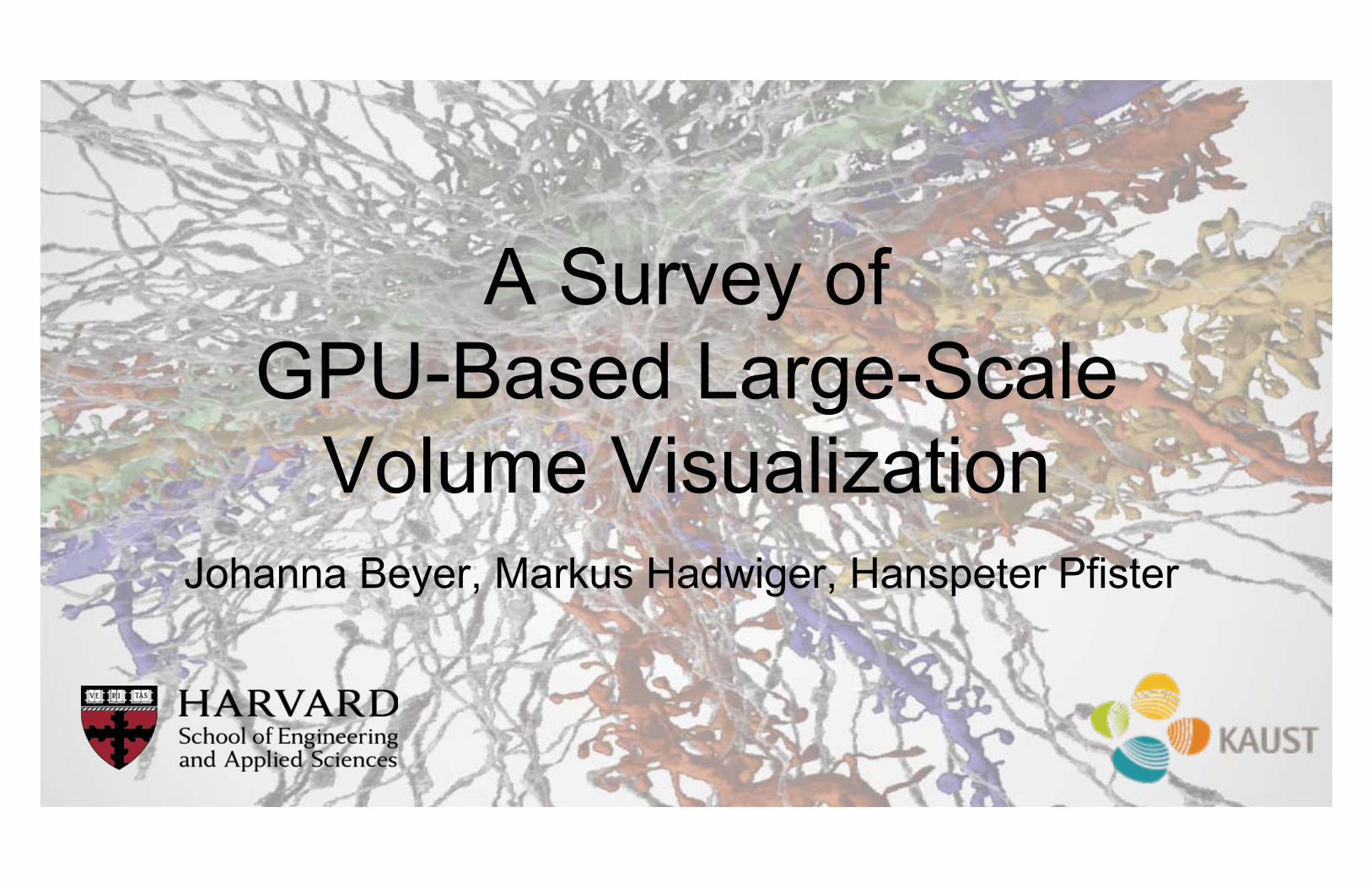
Overview • Part 1: More tutorial material (Markus)

• Motivation and scope • Fundamentals, basic scalability issues and techniques

•  Data representation, work/data partitioning, work/data reduction

• Part 2: More state of the art material (Johanna) • Scalable volume rendering categorization and examples

•  Working set determination

•  Working set storage and access

•  Rendering (ray traversal)

Motivation and Scope

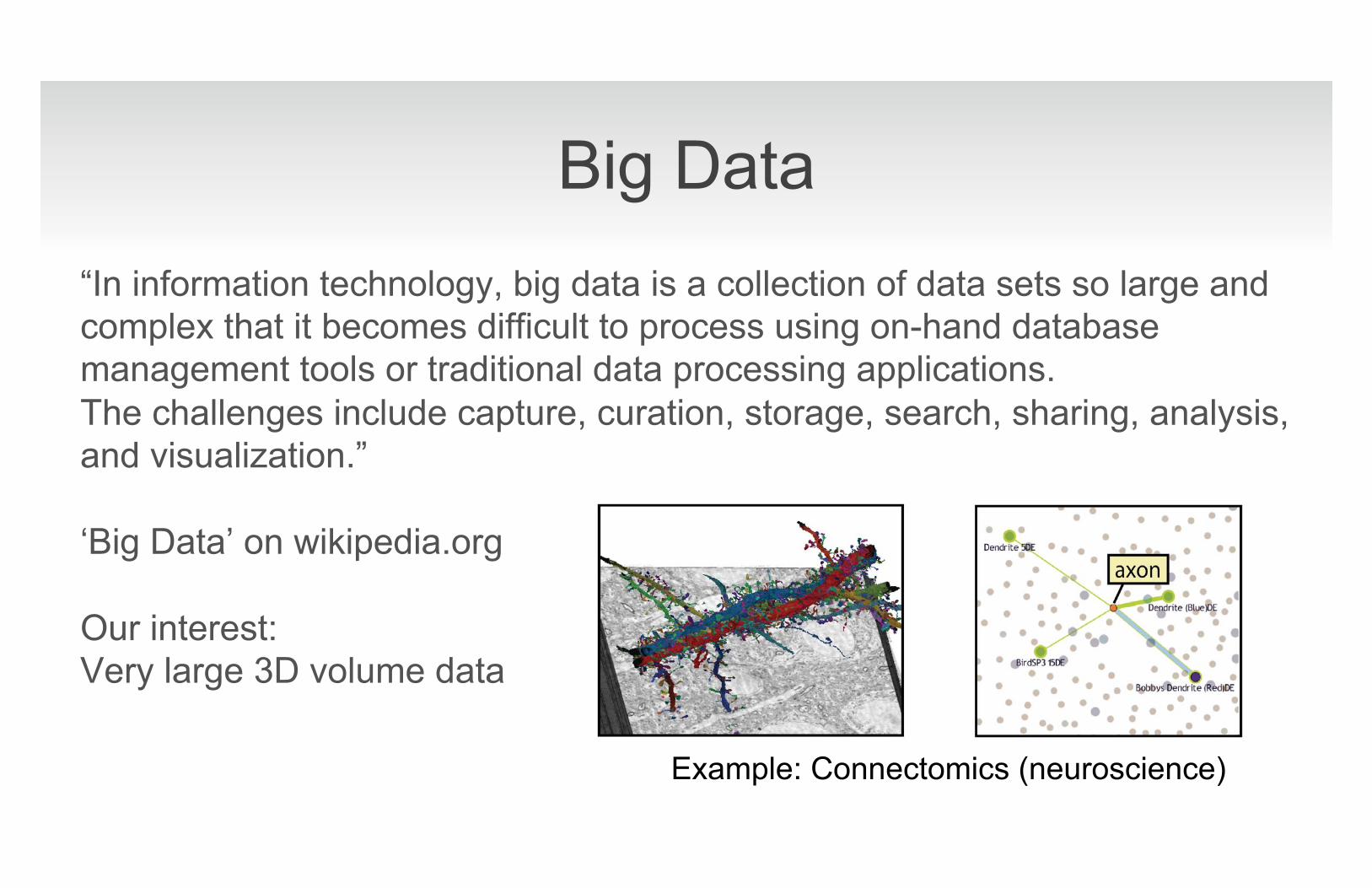
Big Data “In information technology, big data is a collection of data sets so large and complex that it becomes difficult to process using on-hand database management tools or traditional data processing applications. The challenges include capture, curation, storage, search, sharing, analysis, and visualization.” ‘Big Data’ on wikipedia.org Our interest: Very large 3D volume data

Example: Connectomics (neuroscience)

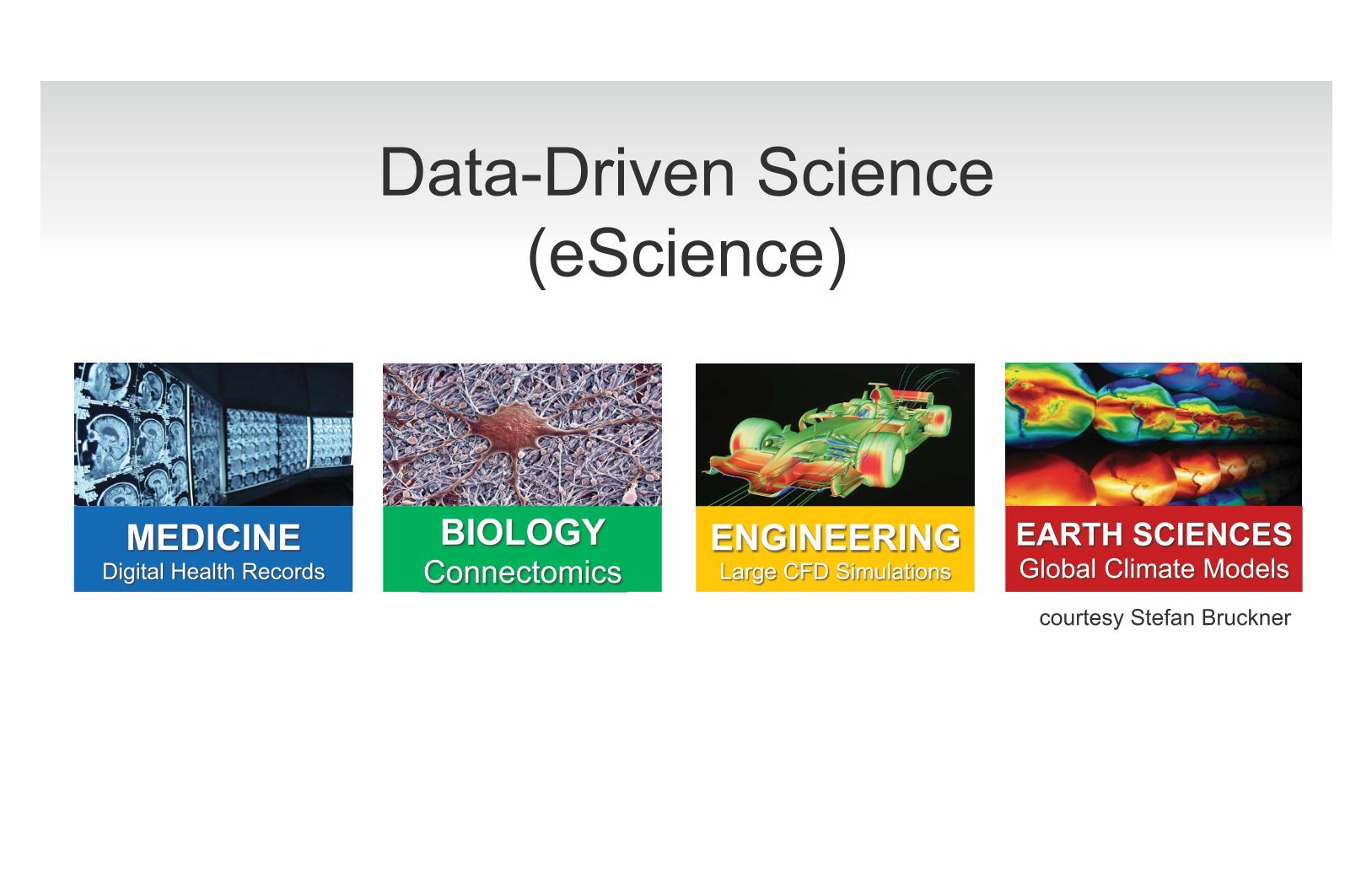
Data-Driven Science (eScience)

EARTH SCIENCES Global Climate Models

MEDICINE Digital Health Records

BIOLOGY Connectomics

ENGINEERING Large CFD Simulations

courtesy Stefan Bruckner

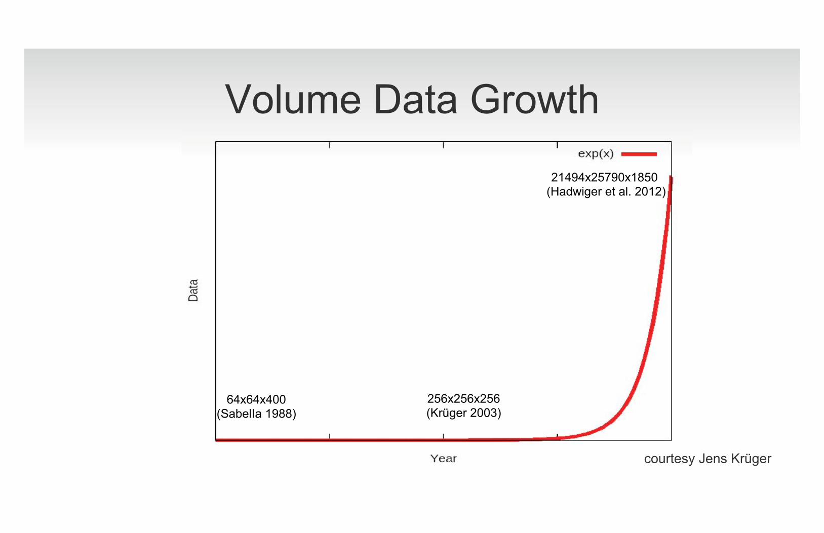
Volume Data Growth

64x64x400 (SabelIa 1988)

21494x25790x1850 (Hadwiger et al. 2012)

256x256x256 (Krüger 2003)

courtesy Jens Krüger

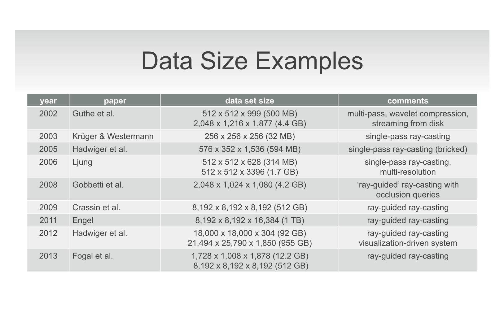
Data Size Examples year paper data set size comments 2002 Guthe et al. 512 x 512 x 999 (500 MB)

2,048 x 1,216 x 1,877 (4.4 GB) multi-pass, wavelet compression,

streaming from disk 2003 Krüger & Westermann 256 x 256 x 256 (32 MB) single-pass ray-casting 2005 Hadwiger et al. 576 x 352 x 1,536 (594 MB) single-pass ray-casting (bricked) 2006 Ljung 512 x 512 x 628 (314 MB)

512 x 512 x 3396 (1.7 GB) single-pass ray-casting,

multi-resolution 2008 Gobbetti et al. 2,048 x 1,024 x 1,080 (4.2 GB) ‘ray-guided’ ray-casting with

occlusion queries 2009 Crassin et al. 8,192 x 8,192 x 8,192 (512 GB) ray-guided ray-casting 2011 Engel 8,192 x 8,192 x 16,384 (1 TB) ray-guided ray-casting 2012 Hadwiger et al. 18,000 x 18,000 x 304 (92 GB)

21,494 x 25,790 x 1,850 (955 GB) ray-guided ray-casting

visualization-driven system 2013 Fogal et al. 1,728 x 1,008 x 1,878 (12.2 GB)

8,192 x 8,192 x 8,192 (512 GB) ray-guided ray-casting

The Connectome�How is the Mammalian Brain Wired?�

Daniel Berger, MIT

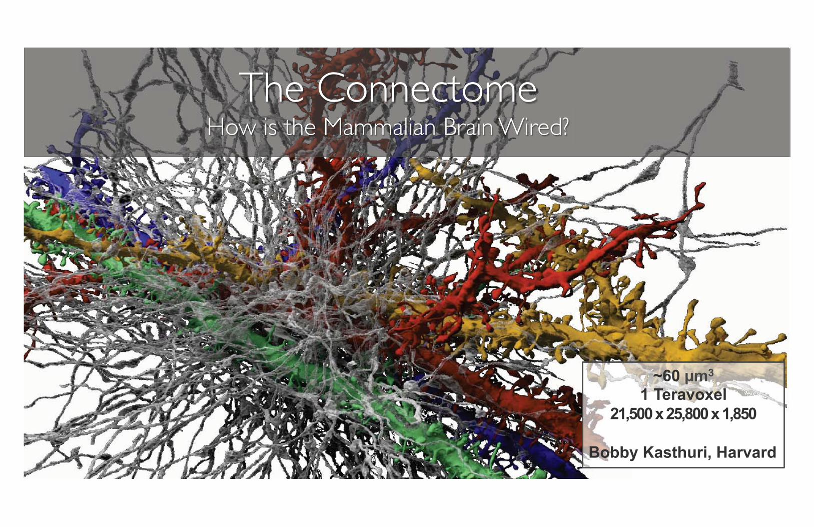
The Connectome�How is the Mammalian Brain Wired?�

~60 µm3

1 Teravoxel 21,500 x 25,800 x 1,850

Bobby Kasthuri, Harvard

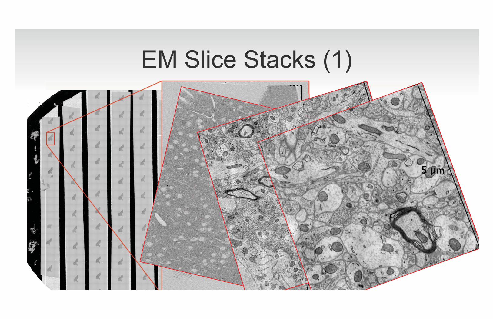
EM Slice Stacks (1)

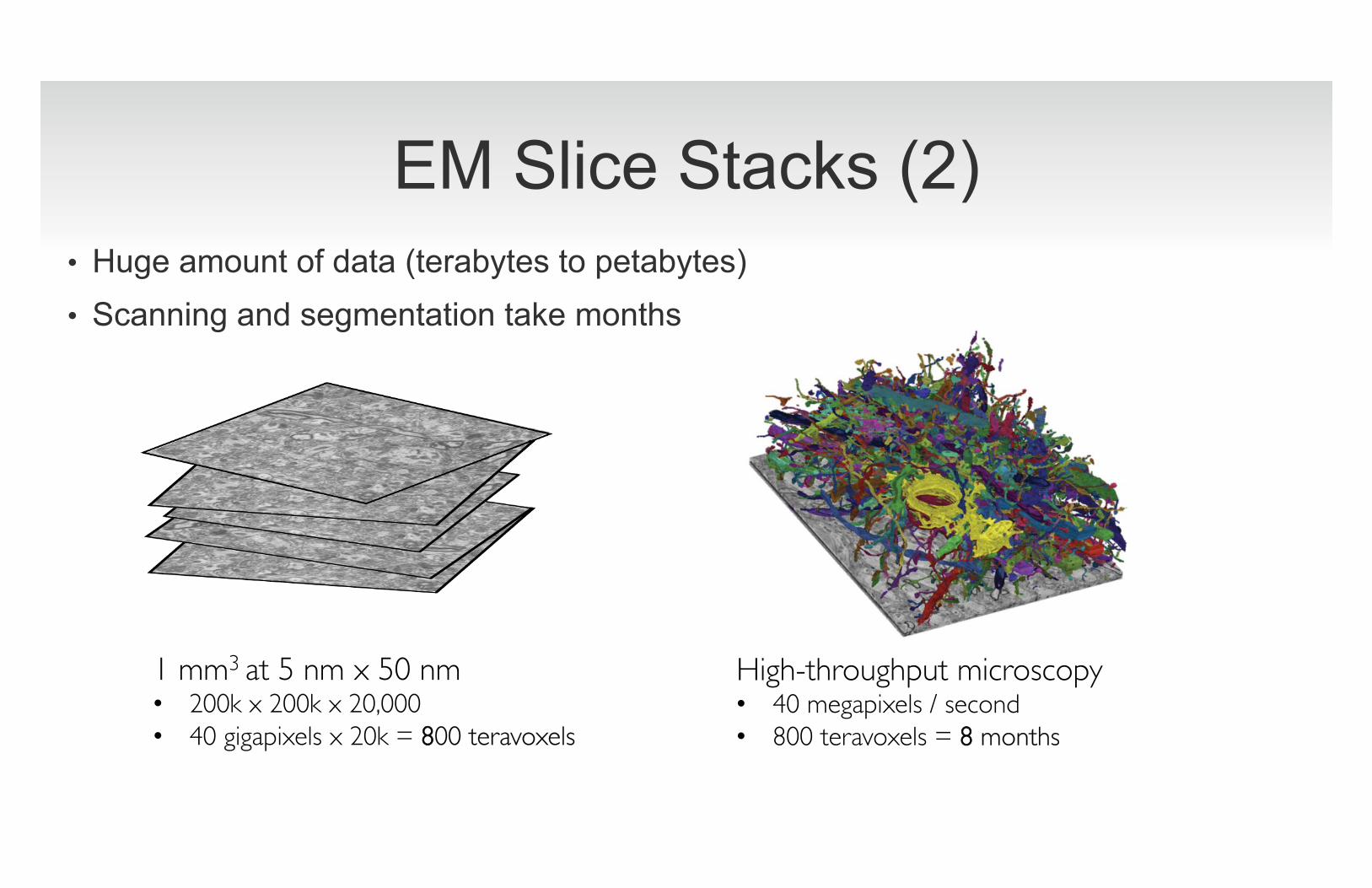
EM Slice Stacks (2) •  Huge amount of data (terabytes to petabytes) •  Scanning and segmentation take months

High-throughput microscopy�•  40 megapixels / second�•  800 teravoxels = 88 months�

1 mm3 at 5 nm x 50 nm�•  200k x 200k x 20,000�•  40 gigapixels x 20k = 8800 teravoxels�

Survey Scope • Focus

•  (Single) GPUs in standard workstations • Scalar volume data; single time step • But a lot applies to more general settings�

• Orthogonal techniques (won’t cover details) • Parallel and distributed rendering, clusters, supercomputers, � • Compression

Related Books and Surveys • Books

•  Real-Time Volume Graphics, Engel et al., 2006

•  High-Performance Visualization, Bethel et al., 2012

• Surveys •  Parallel Visualization: Wittenbrink ’98, Bartz et al. ‘00, Zhang et al. ’05

•  Real Time Interactive Massive Model Visualization: Kasik et al. ‘06 •  Vis and Visual Analysis of Multifaceted Scientific Data: Kehrer and Hauser ‘13

•  Compressed GPU-Based Volume Rendering: Rodriguez et al. ‘13

Fundamentals

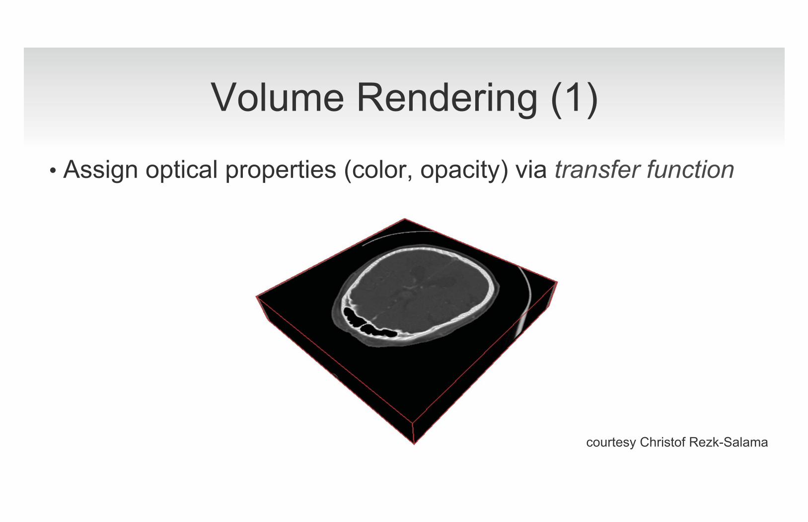
Volume Rendering (1)

• Assign optical properties (color, opacity) via transfer function

courtesy Christof Rezk-Salama

Volume Rendering (2)

• Ray-casting

courtesy Christof Rezk-Salama

Scalability

• Traditional HPC, parallel rendering definitions • Strong scaling (“more nodes are faster for same data”) • Weak scaling (“more nodes allow larger data”)

• Our interest/definition: output sensitivity • Running time/storage proportional to size of output instead of input

•  Computational effort scales with visible data and screen resolution�

•  Working set independent of original data size�

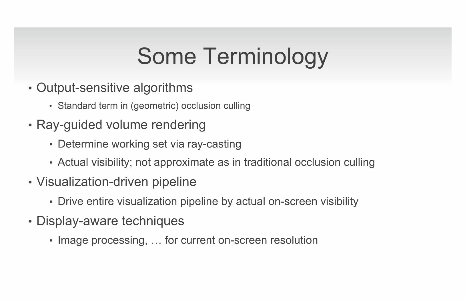
Some Terminology • Output-sensitive algorithms

•  Standard term in (geometric) occlusion culling

• Ray-guided volume rendering •  Determine working set via ray-casting •  Actual visibility; not approximate as in traditional occlusion culling

• Visualization-driven pipeline •  Drive entire visualization pipeline by actual on-screen visibility

• Display-aware techniques •  Image processing, � for current on-screen resolution

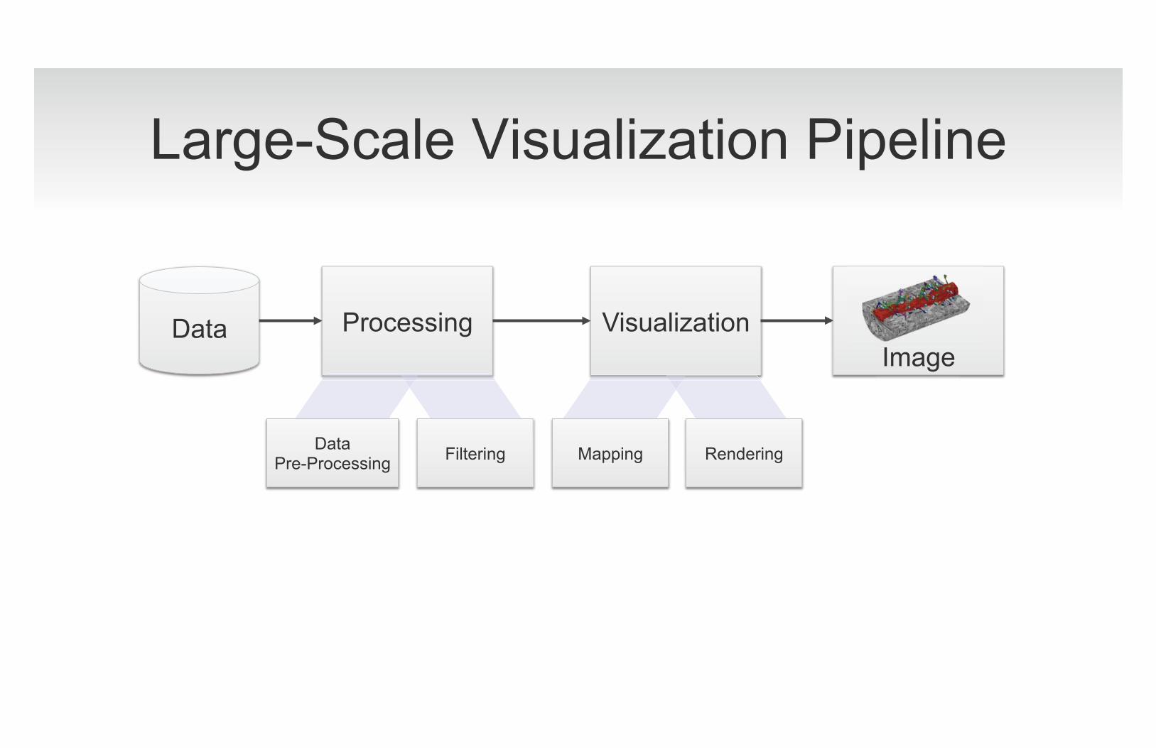
Large-Scale Visualization Pipeline

Data Processing Visualization

Image

Filtering Mapping Rendering Data Pre-Processing

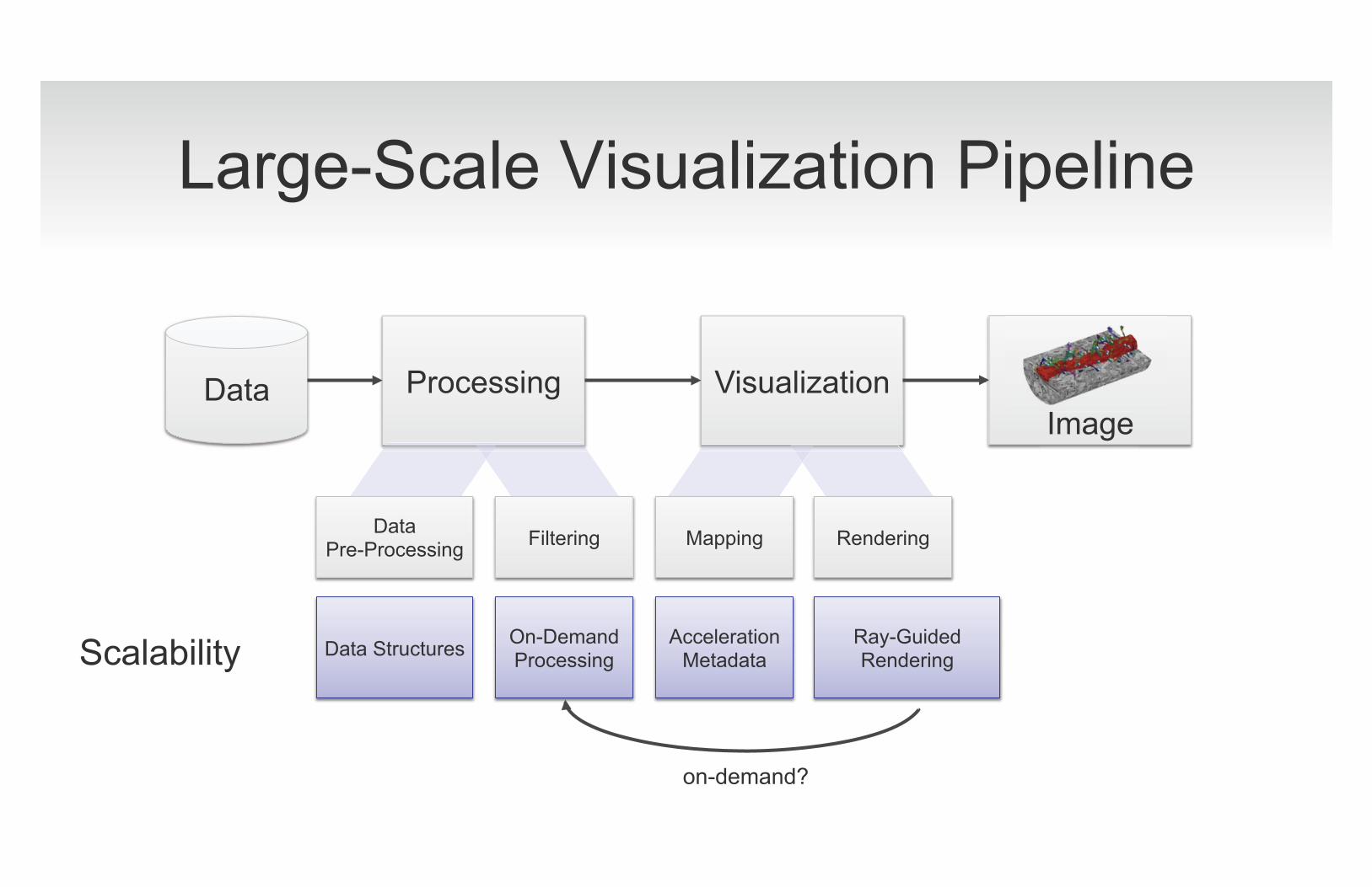
Large-Scale Visualization Pipeline

Data Processing Visualization

Image

Filtering Data Pre-Processing

Ray-Guided Rendering Data Structures Acceleration

Metadata On-Demand Processing

on-demand?

Scalability

Mapping Rendering

Basic Scalability Issues

Scalability Issues Scalability issues Scalable method Data representation and storage Multi-resolution data structures

Data layout, compression Work/data partitioning In-core/out-of-core

Parallel, distributed Work/data reduction Pre-processing

On-demand processing Streaming In-situ visualization Query-based visualization

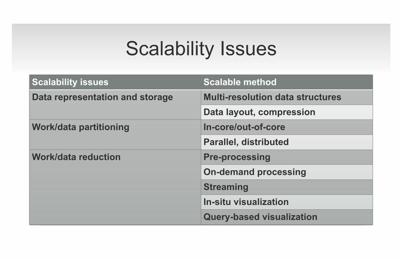
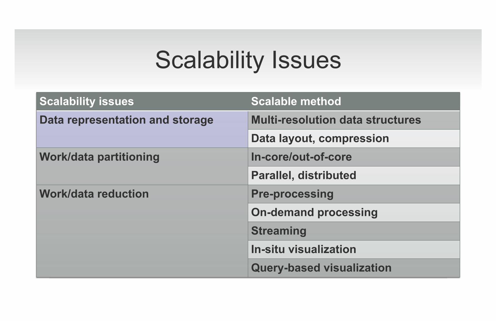
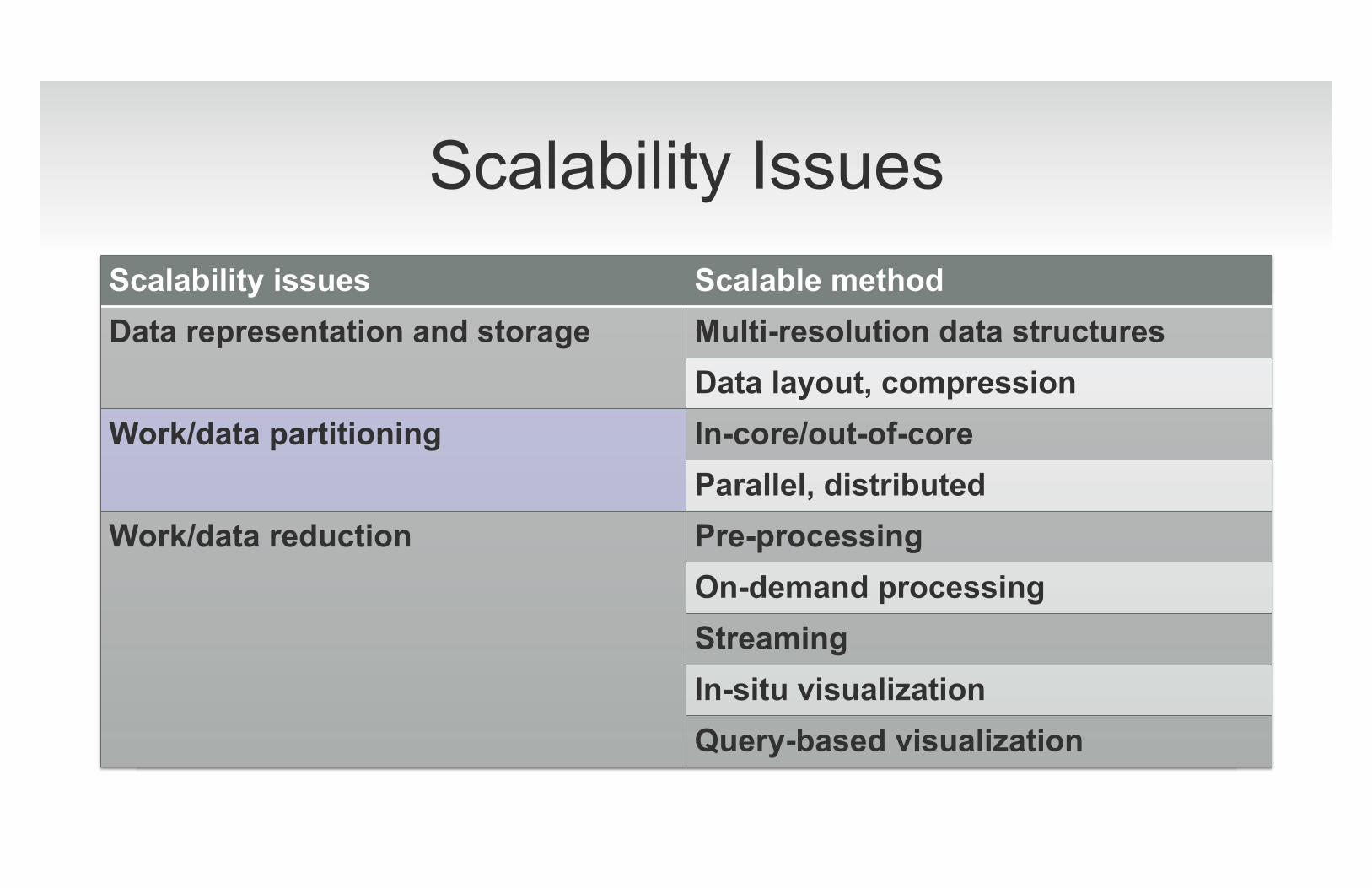
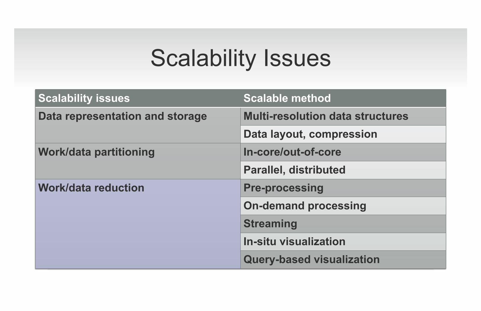
Scalability Issues Scalability issues Scalable method Data representation and storage Multi-resolution data structures

Data layout, compression Work/data partitioning In-core/out-of-core

Parallel, distributed Work/data reduction Pre-processing

On-demand processing Streaming In-situ visualization Query-based visualization

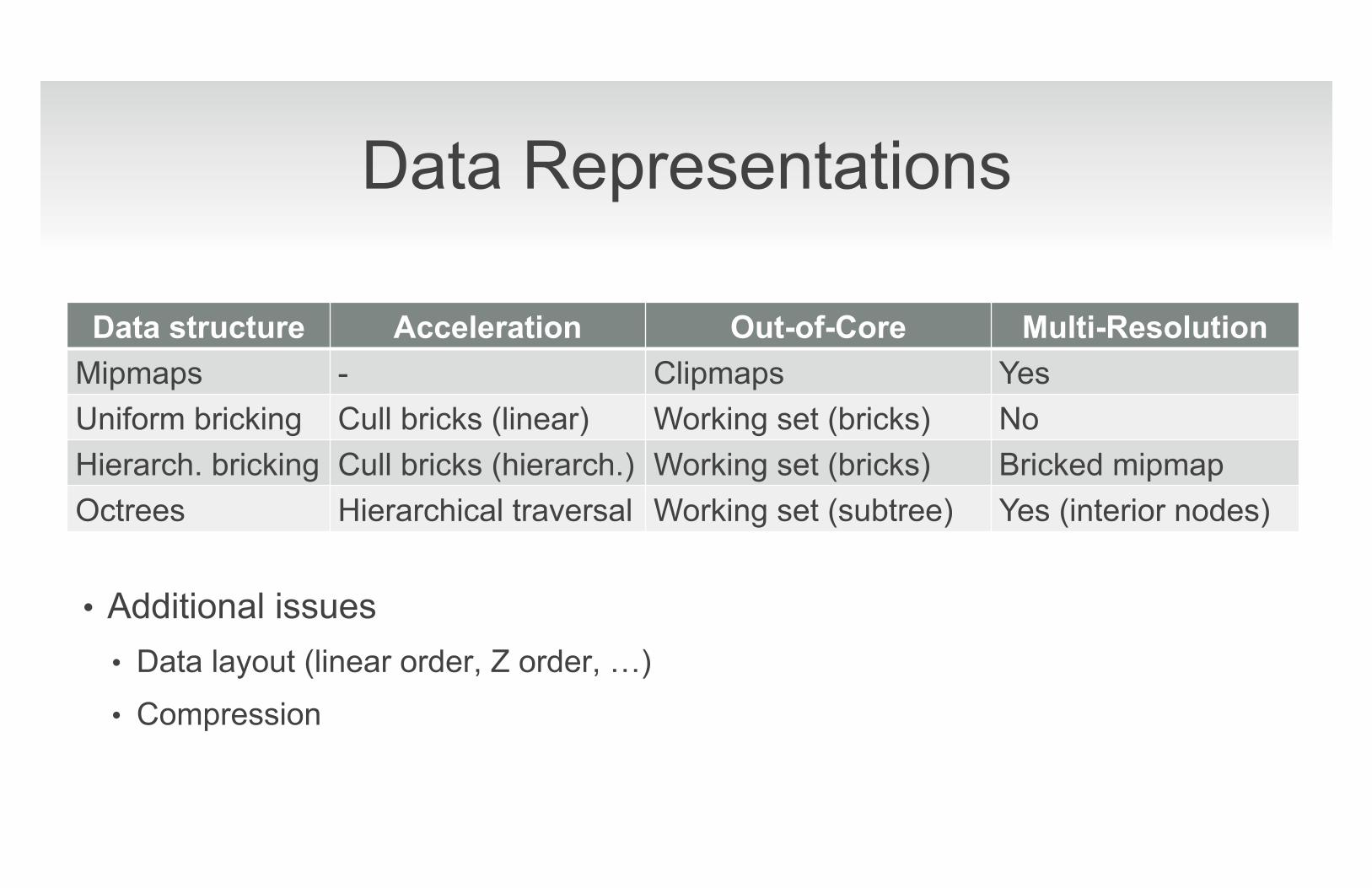
• Additional issues •  Data layout (linear order, Z order, �)

•  Compression

Data Representations

Data structure Acceleration Out-of-Core Multi-Resolution Mipmaps - Clipmaps Yes Uniform bricking Cull bricks (linear) Working set (bricks) No Hierarch. bricking Cull bricks (hierarch.) Working set (bricks) Bricked mipmap Octrees Hierarchical traversal Working set (subtree) Yes (interior nodes)

Uniform vs. Hierarchical Decomposition

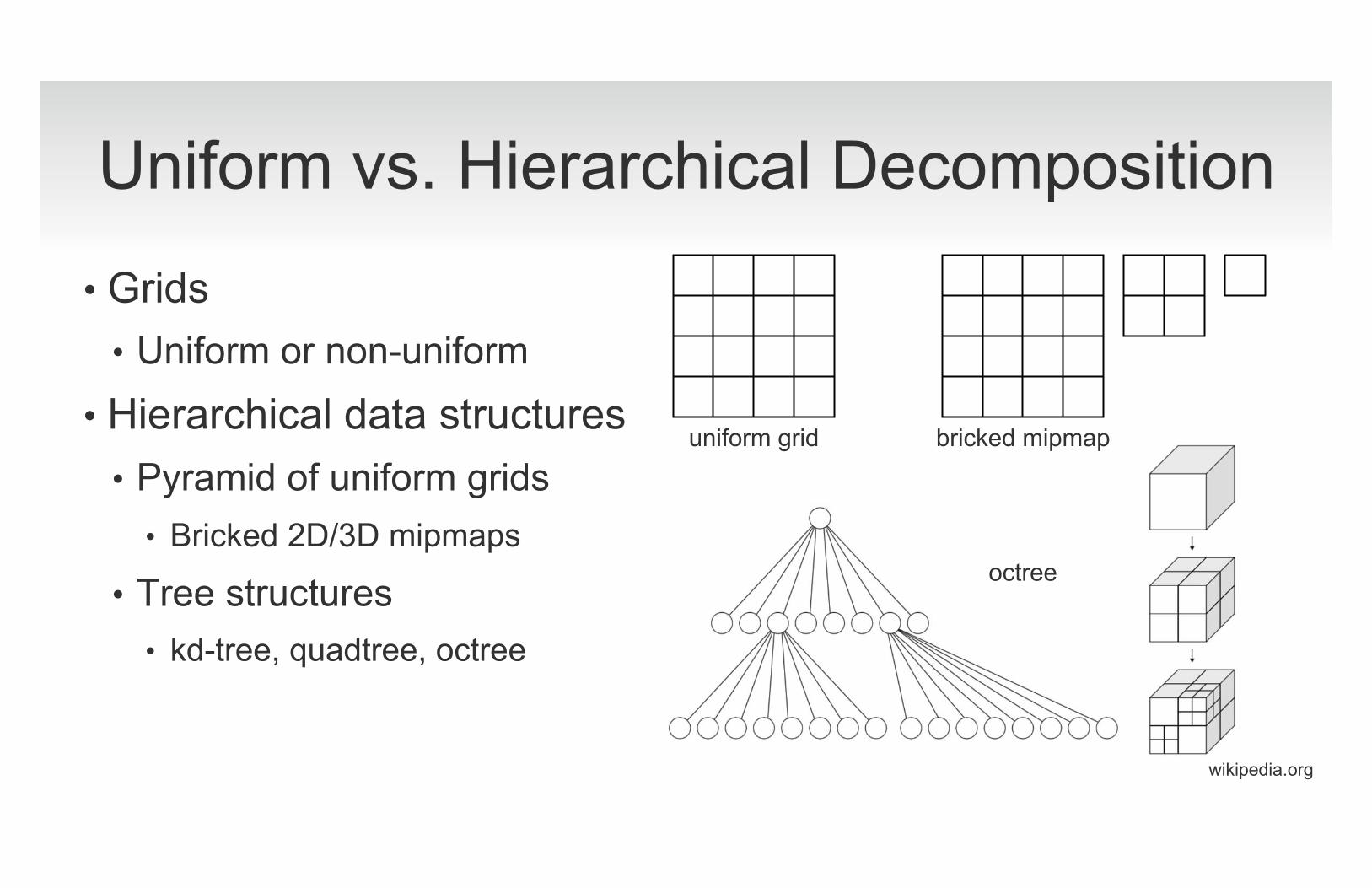
• Grids • Uniform or non-uniform

• Hierarchical data structures • Pyramid of uniform grids

•  Bricked 2D/3D mipmaps

• Tree structures •  kd-tree, quadtree, octree

uniform grid bricked mipmap

octree

wikipedia.org

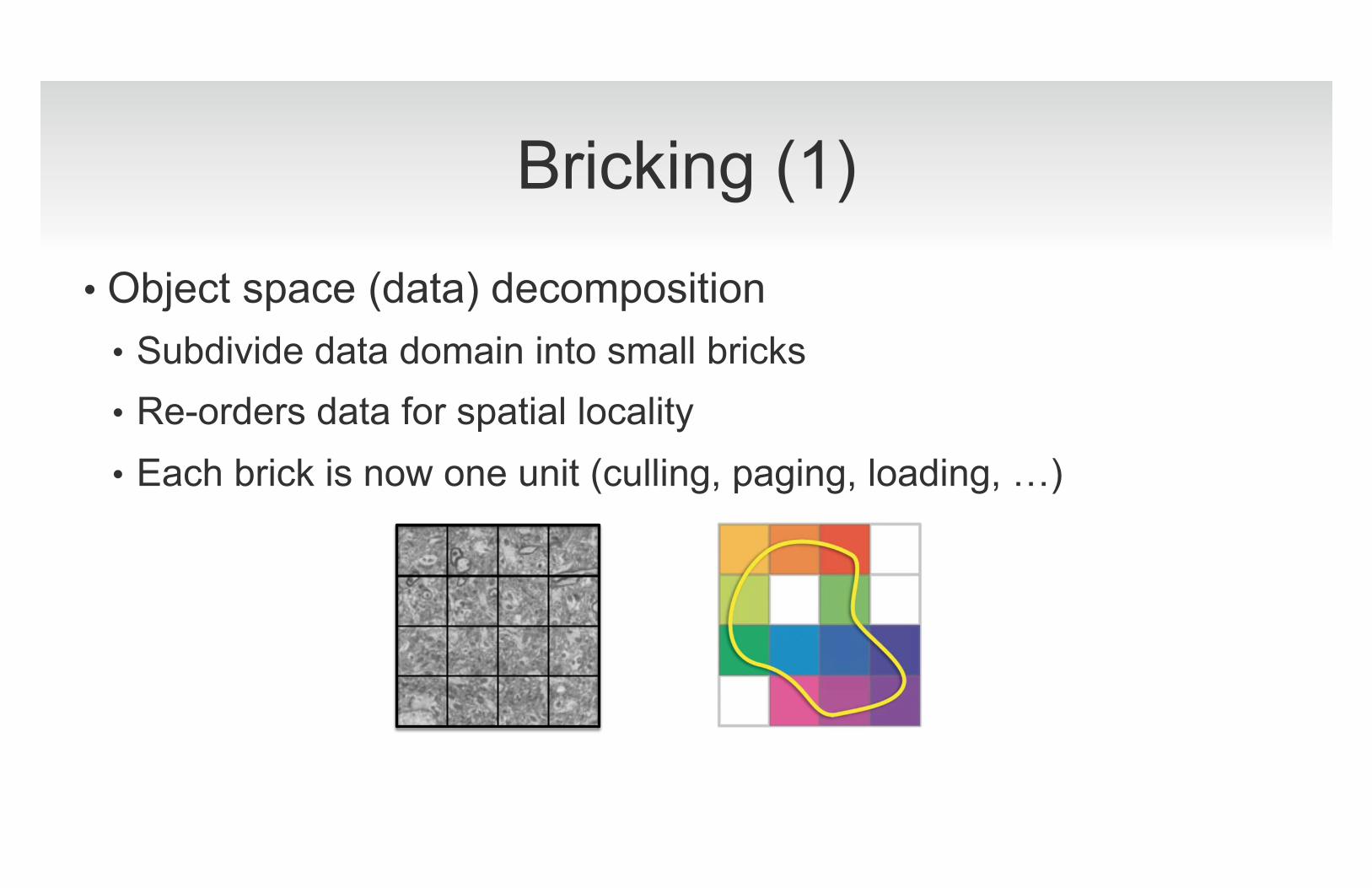
Bricking (1)

• Object space (data) decomposition • Subdivide data domain into small bricks • Re-orders data for spatial locality • Each brick is now one unit (culling, paging, loading, �)

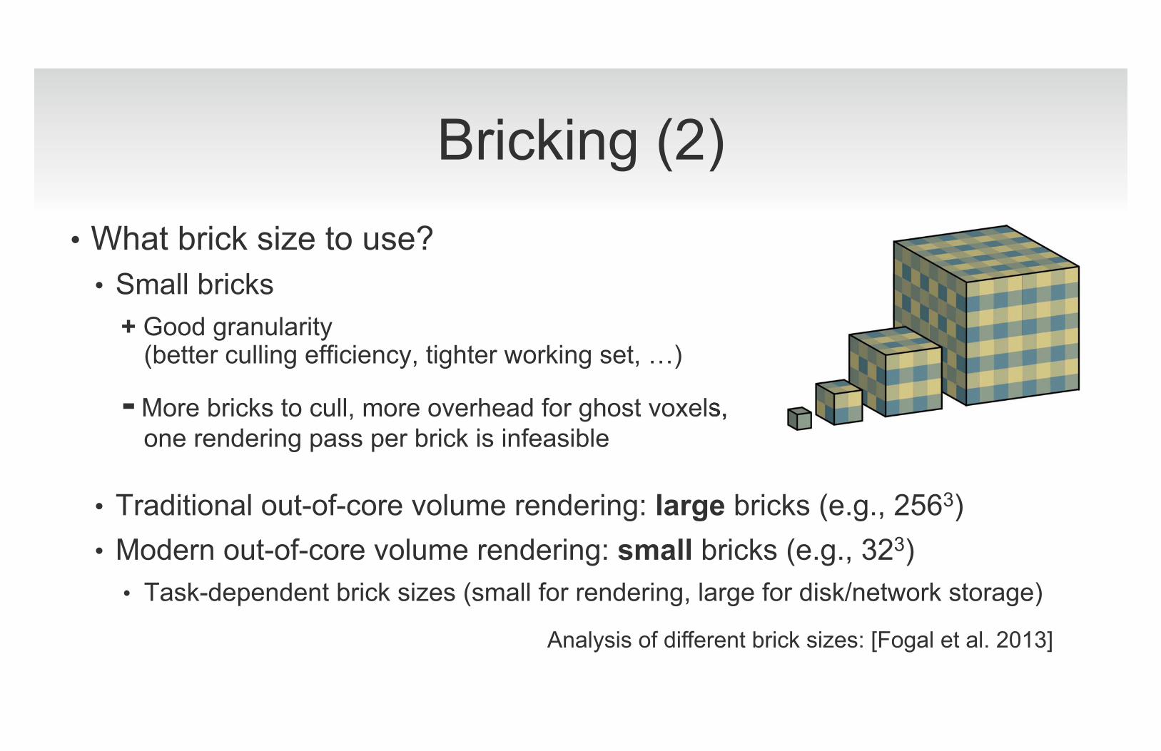
Bricking (2) • What brick size to use?

•  Small bricks + Good granularity

(better culling efficiency, tighter working set, �)

- More bricks to cull, more overhead for ghost voxels, one rendering pass per brick is infeasible

•  Traditional out-of-core volume rendering: large bricks (e.g., 2563) • Modern out-of-core volume rendering: small bricks (e.g., 323)

•  Task-dependent brick sizes (small for rendering, large for disk/network storage) Analysis of different brick sizes: [Fogal et al. 2013]

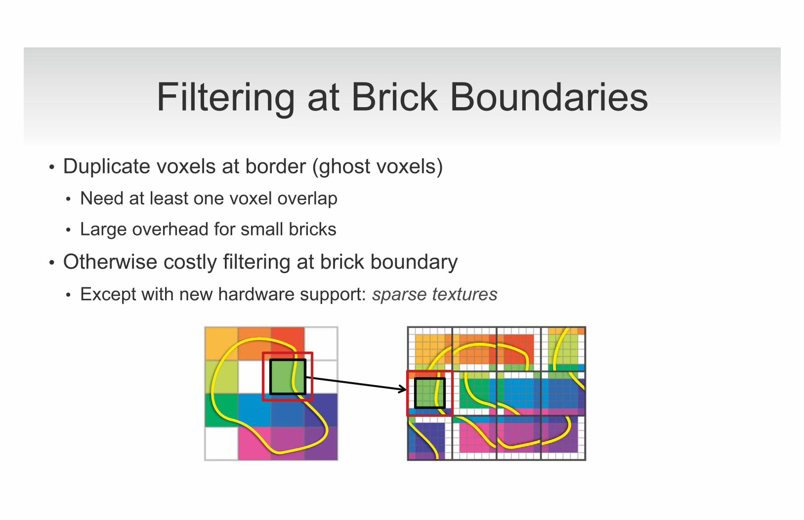
Filtering at Brick Boundaries • Duplicate voxels at border (ghost voxels)

•  Need at least one voxel overlap

•  Large overhead for small bricks

• Otherwise costly filtering at brick boundary •  Except with new hardware support: sparse textures

Pre-Compute All Bricks?

• Pre-computation might take very long • Brick on demand? Brick in streaming fashion (e.g., during scanning)?

• Different brick sizes for different tasks (storage, rendering)? • Re-brick to different size on demand? • Dynamically fix up ghost voxels?

• Can also mix 2D and 3D • E.g., 2D tiling pre-computed, but compute 3D bricks on demand

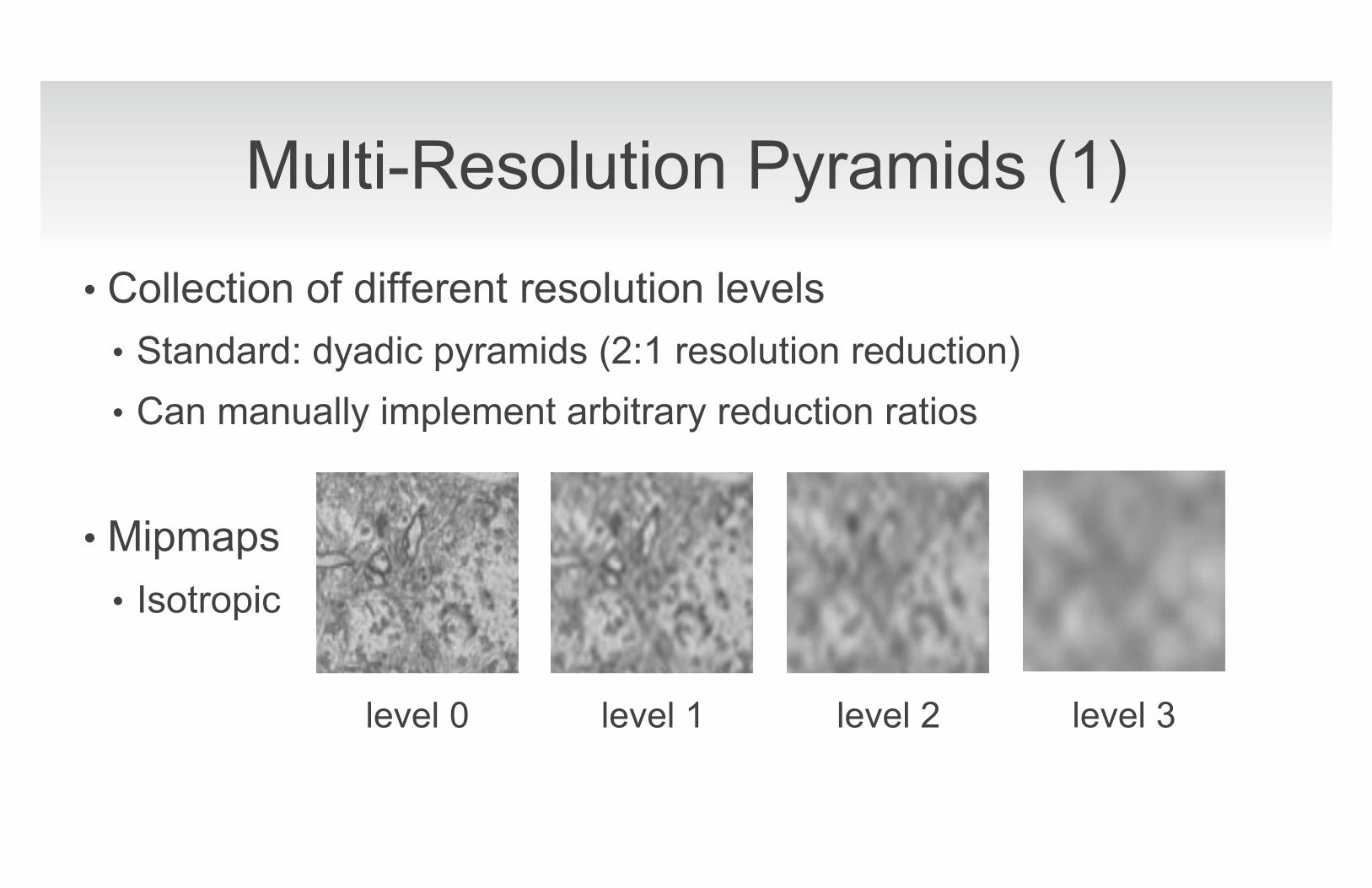
Multi-Resolution Pyramids (1)

• Collection of different resolution levels • Standard: dyadic pyramids (2:1 resolution reduction) • Can manually implement arbitrary reduction ratios

• Mipmaps •  Isotropic

level 0 level 1 level 2 level 3

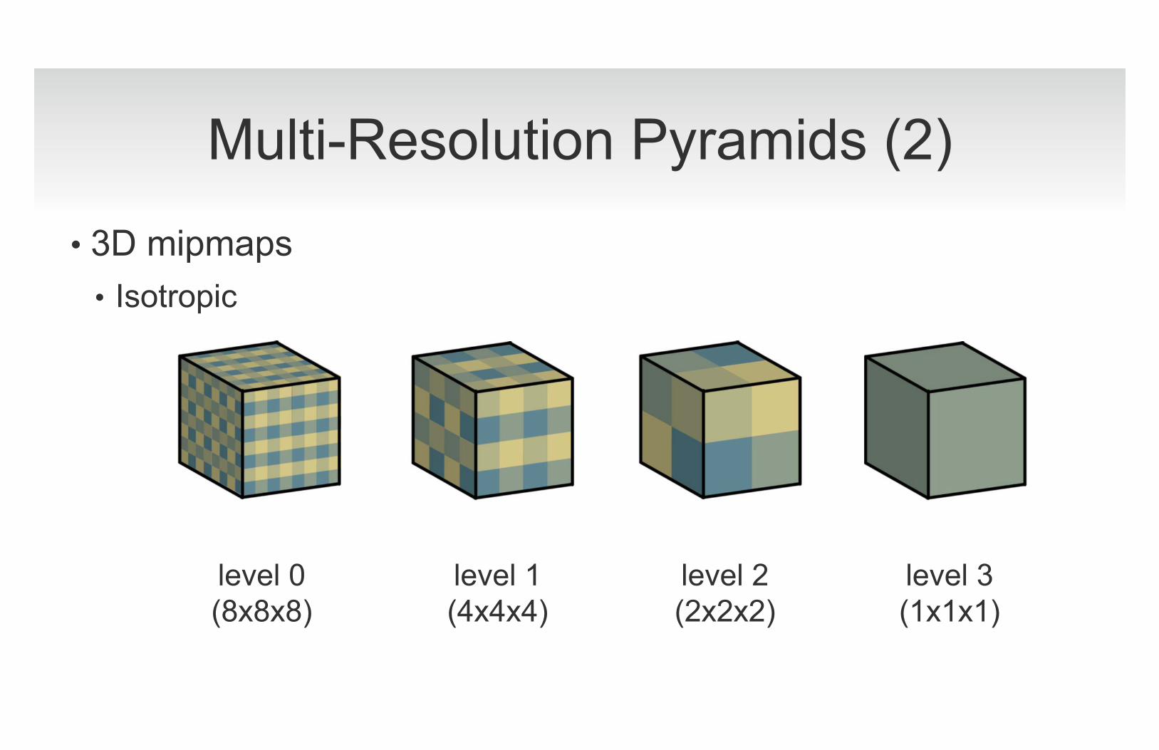
Multi-Resolution Pyramids (2)

• 3D mipmaps •  Isotropic

level 0 (8x8x8)

level 1 (4x4x4)

level 2 (2x2x2)

level 3 (1x1x1)

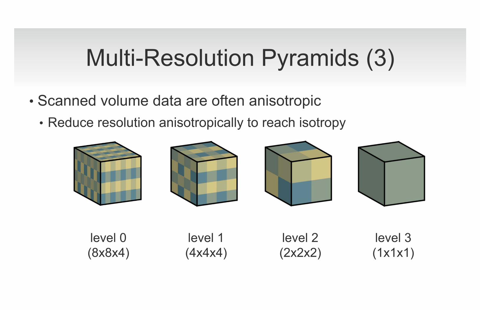
Multi-Resolution Pyramids (3)

• Scanned volume data are often anisotropic • Reduce resolution anisotropically to reach isotropy

level 0 (8x8x4)

level 1 (4x4x4)

level 2 (2x2x2)

level 3 (1x1x1)

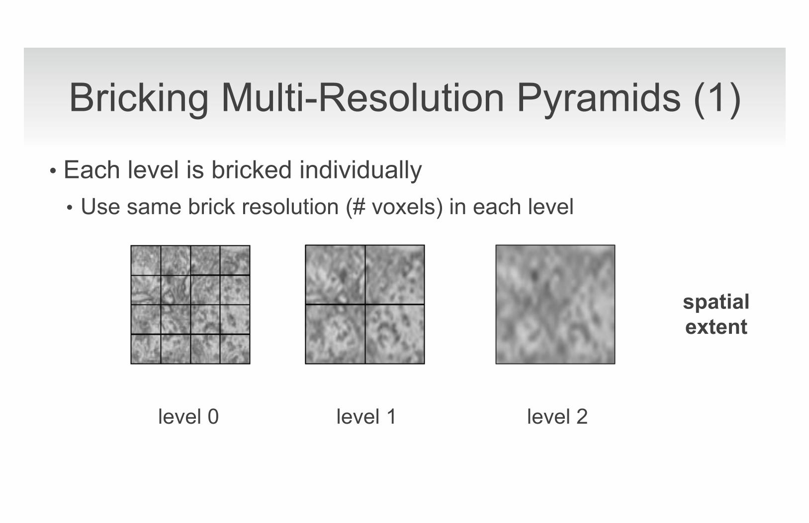
Bricking Multi-Resolution Pyramids (1)

• Each level is bricked individually • Use same brick resolution (# voxels) in each level

spatial extent

level 0 level 1 level 2

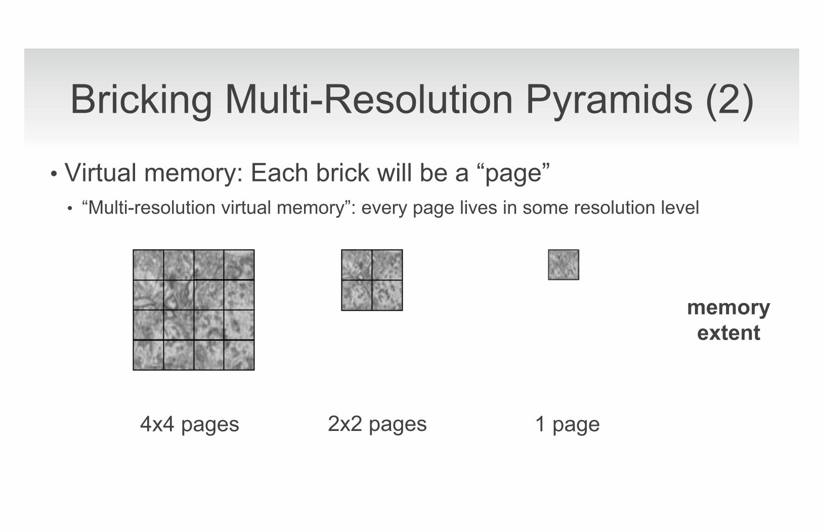
Bricking Multi-Resolution Pyramids (2)

• Virtual memory: Each brick will be a “page” •  “Multi-resolution virtual memory”: every page lives in some resolution level

4x4 pages 1 page

memory extent

2x2 pages

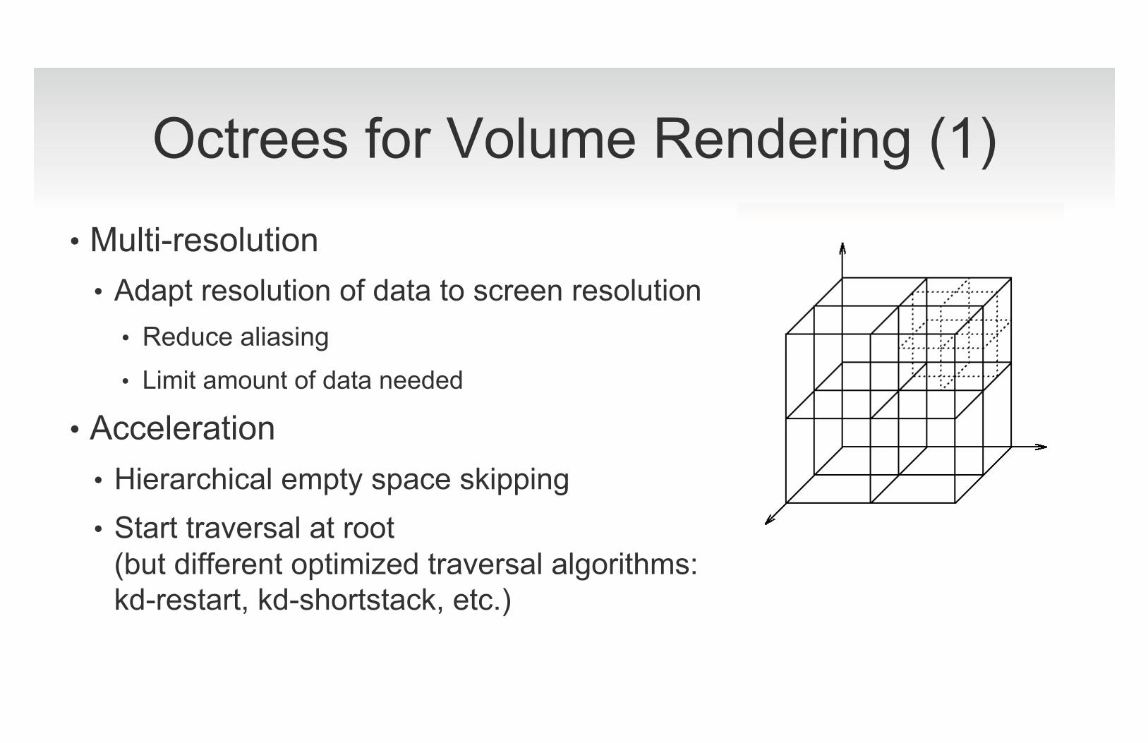
Octrees for Volume Rendering (1) • Multi-resolution

• Adapt resolution of data to screen resolution •  Reduce aliasing •  Limit amount of data needed

• Acceleration • Hierarchical empty space skipping • Start traversal at root

(but different optimized traversal algorithms: kd-restart, kd-shortstack, etc.)

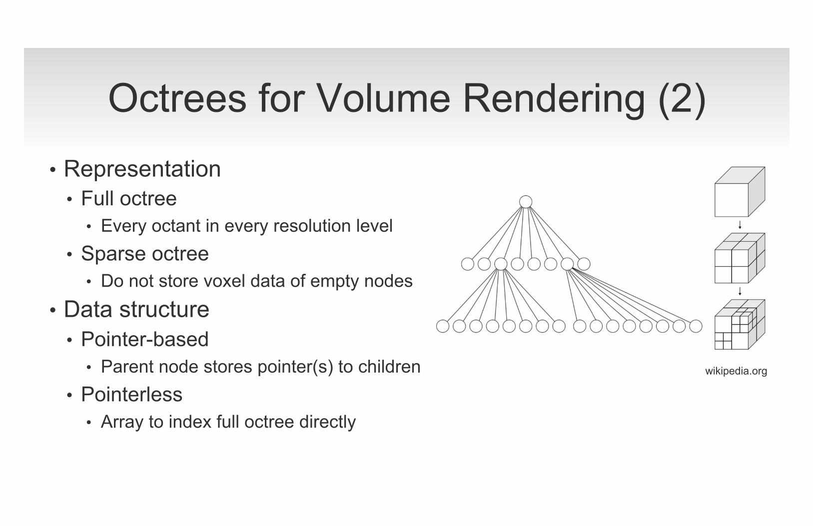
Octrees for Volume Rendering (2) • Representation

•  Full octree •  Every octant in every resolution level

•  Sparse octree •  Do not store voxel data of empty nodes

• Data structure •  Pointer-based

•  Parent node stores pointer(s) to children •  Pointerless

•  Array to index full octree directly

wikipedia.org

Scalability Issues Scalability issues Scalable method Data representation and storage Multi-resolution data structures

Data layout, compression Work/data partitioning In-core/out-of-core

Parallel, distributed Work/data reduction Pre-processing

On-demand processing Streaming In-situ visualization Query-based visualization

Work/Data Partitioning

• Out-of-core techniques • Domain decomposition • Parallel and distributed rendering

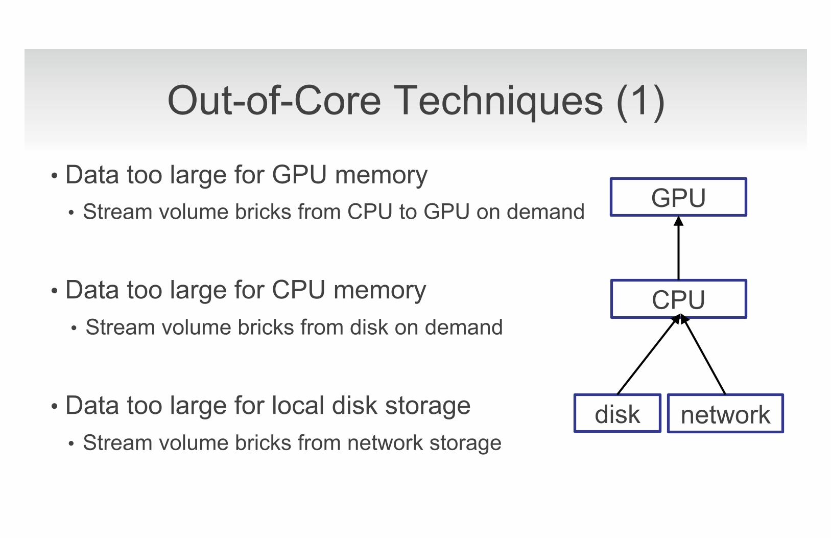
Out-of-Core Techniques (1)

• Data too large for GPU memory • Stream volume bricks from CPU to GPU on demand

• Data too large for CPU memory • Stream volume bricks from disk on demand

• Data too large for local disk storage • Stream volume bricks from network storage

GPU

CPU

disk network

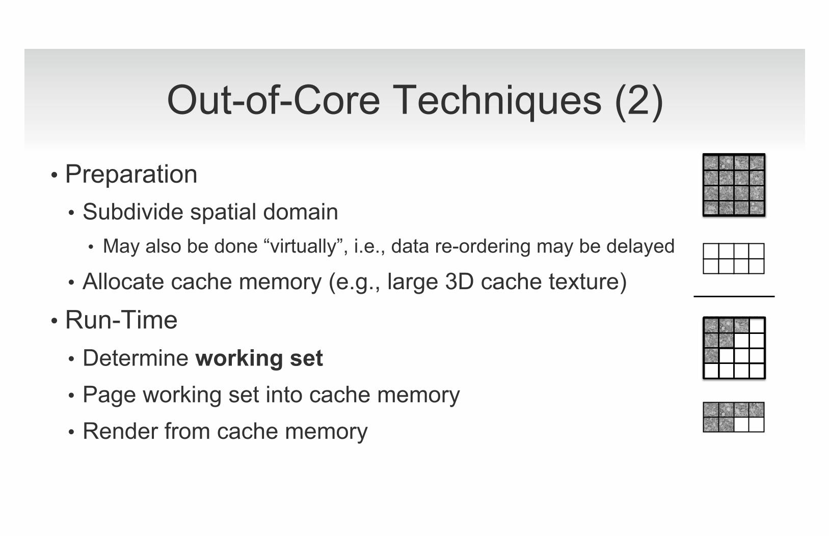
• Preparation • Subdivide spatial domain

•  May also be done “virtually”, i.e., data re-ordering may be delayed

• Allocate cache memory (e.g., large 3D cache texture)

• Run-Time • Determine working set • Page working set into cache memory • Render from cache memory

Out-of-Core Techniques (2)

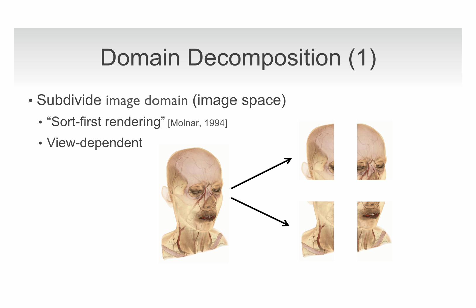
Domain Decomposition (1)

• Subdivide image domain (image space) •  “Sort-first rendering” [Molnar, 1994]

• View-dependent

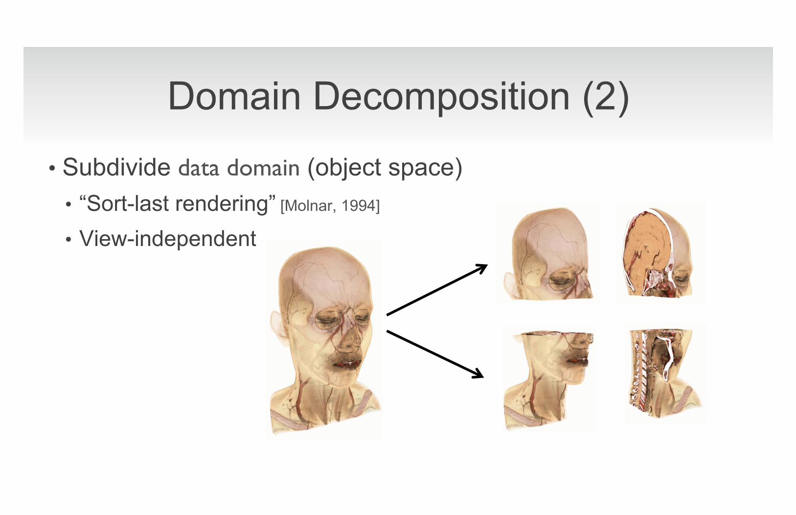
Domain Decomposition (2)

• Subdivide data domain (object space) •  “Sort-last rendering” [Molnar, 1994]

• View-independent

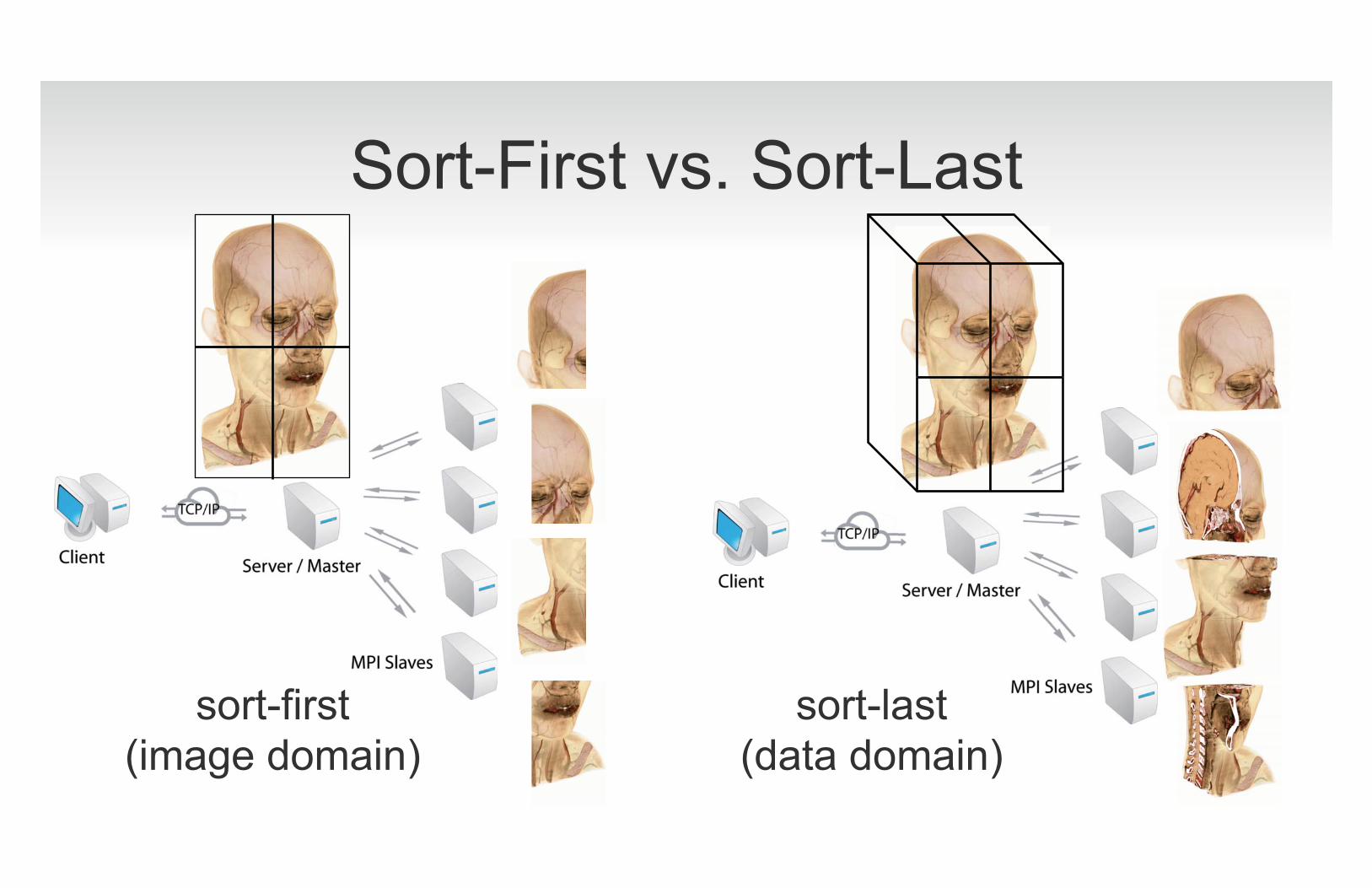
Sort-First vs. Sort-Last

sort-first (image domain)

sort-last (data domain)

Scalability Issues Scalability issues Scalable method Data representation and storage Multi-resolution data structures

Data layout, compression Work/data partitioning In-core/out-of-core

Parallel, distributed Work/data reduction Pre-processing

On-demand processing Streaming In-situ visualization Query-based visualization

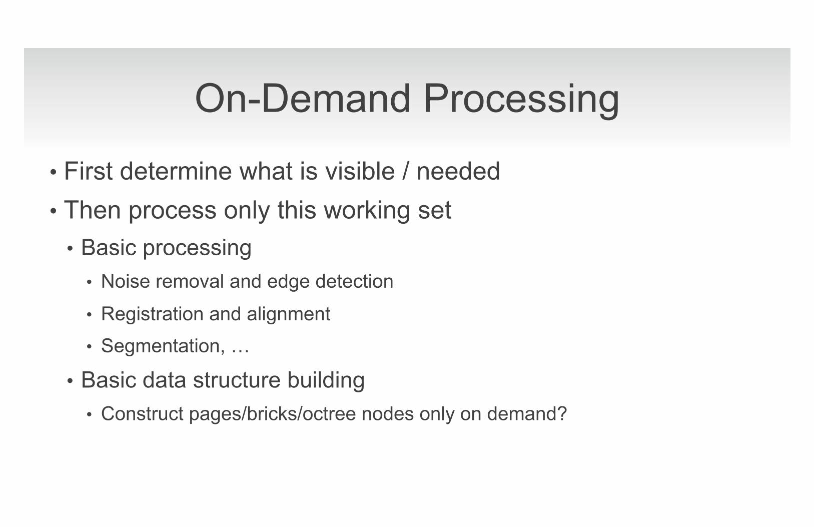
On-Demand Processing

• First determine what is visible / needed • Then process only this working set

• Basic processing •  Noise removal and edge detection

•  Registration and alignment •  Segmentation, �

• Basic data structure building •  Construct pages/bricks/octree nodes only on demand?

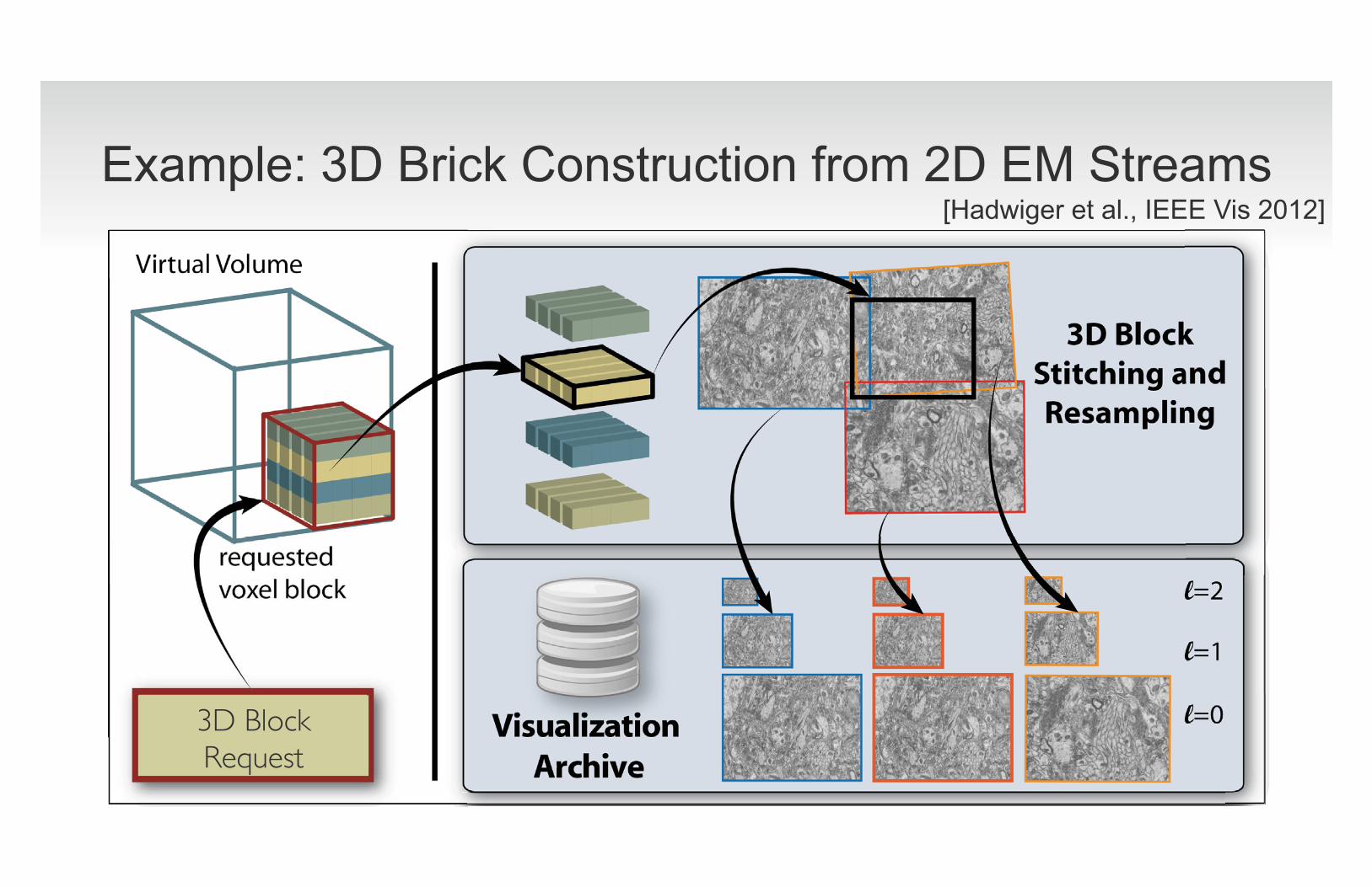
Example: 3D Brick Construction from 2D EM Streams

3D Block �Request�

[Hadwiger et al., IEEE Vis 2012]

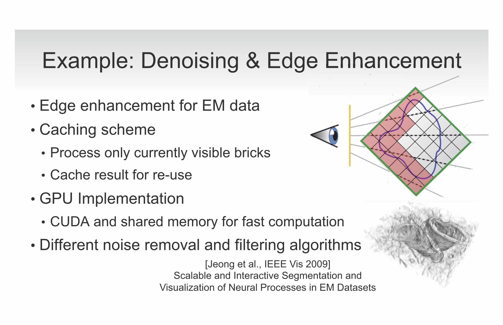
Example: Denoising & Edge Enhancement

• Edge enhancement for EM data • Caching scheme

• Process only currently visible bricks • Cache result for re-use

• GPU Implementation • CUDA and shared memory for fast computation

• Different noise removal and filtering algorithms [Jeong et al., IEEE Vis 2009]

Scalable and Interactive Segmentation and Visualization of Neural Processes in EM Datasets

Example: Registration & Alignment • Registration at screen/brick resolution

[Beyer et al., CG&A 2013] Exploring the Connectome – Petascale Volume

Visualization of Microscopy Data Streams

Questions for Part 1?

Next: (More) Scalable Volume Rendering

THANKS�

Webpage:�http://people.seas.harvard.edu/~jbeyer/star.html�

Part 2 - Scalable Volume Rendering

Part 2 - Scalable Volume Rendering • History

• Categorization

•  Working Set Determination

•  Working Set Storage & Access

•  Rendering (Ray Traversal)

• Ray-Guided Volume Rendering Examples

• Conclusion

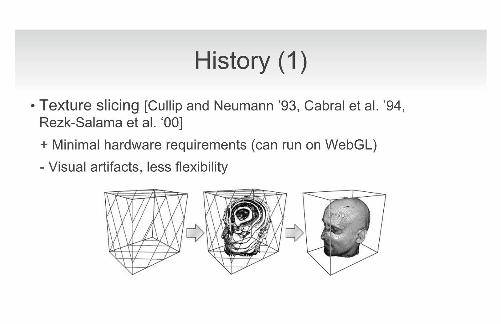
History (1)

• Texture slicing [Cullip and Neumann ’93, Cabral et al. ’94, Rezk-Salama et al. ‘00] + Minimal hardware requirements (can run on WebGL) - Visual artifacts, less flexibility

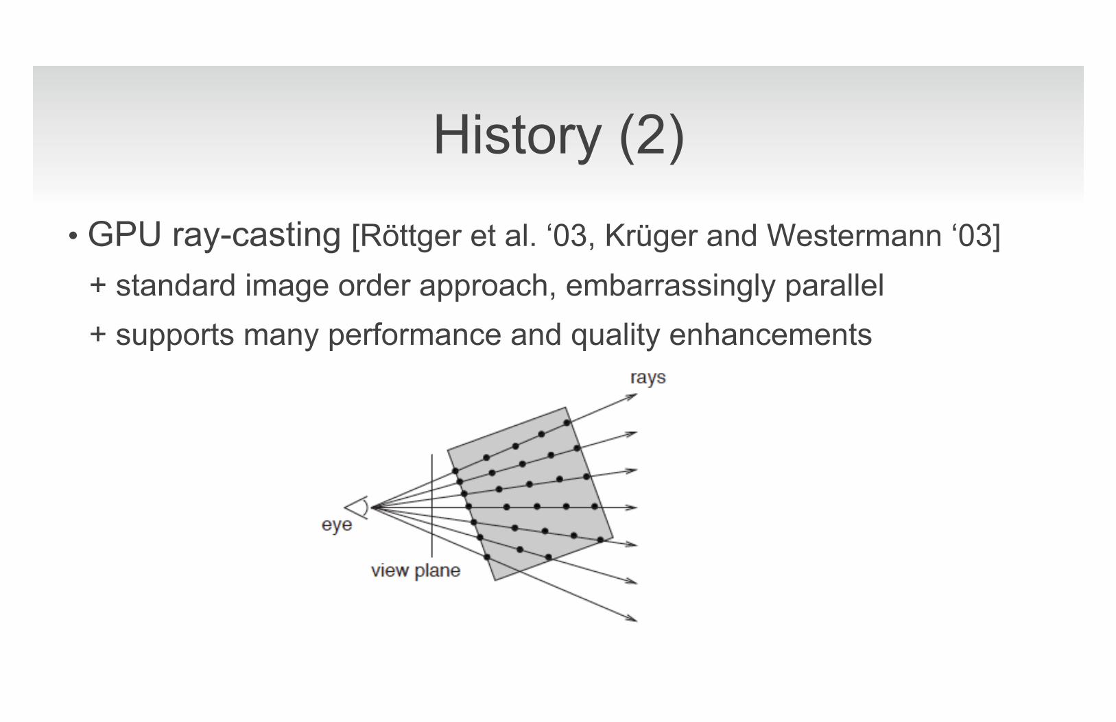
History (2)

• GPU ray-casting [Röttger et al. ‘03, Krüger and Westermann ‘03] + standard image order approach, embarrassingly parallel + supports many performance and quality enhancements

History (3)

• Large data volume rendering • Octree rendering based on texture-slicing

[LaMar et al. ’99, Weiler et al. ’00, Guthe et al. ’02] • Bricked single-pass ray-casting

[Hadwiger et al. ’05, Beyer et al. ’07] • Bricked multi-resolution single-pass ray-casting

[Ljung et al. ’06, Beyer et al. ’08, Jeong et al. ’09] • Optimized CPU ray-casting [Knoll et al. ’11]

Examples

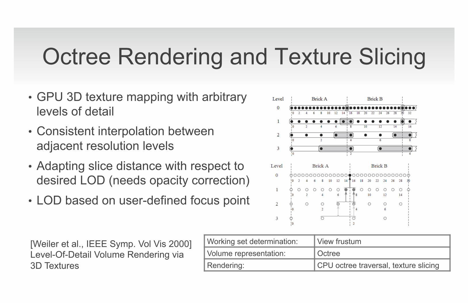
Octree Rendering and Texture Slicing • GPU 3D texture mapping with arbitrary

levels of detail • Consistent interpolation between

adjacent resolution levels • Adapting slice distance with respect to

desired LOD (needs opacity correction) •  LOD based on user-defined focus point

[Weiler et al., IEEE Symp. Vol Vis 2000] Level-Of-Detail Volume Rendering via 3D Textures

Working set determination: View frustum Volume representation: Octree Rendering: CPU octree traversal, texture slicing

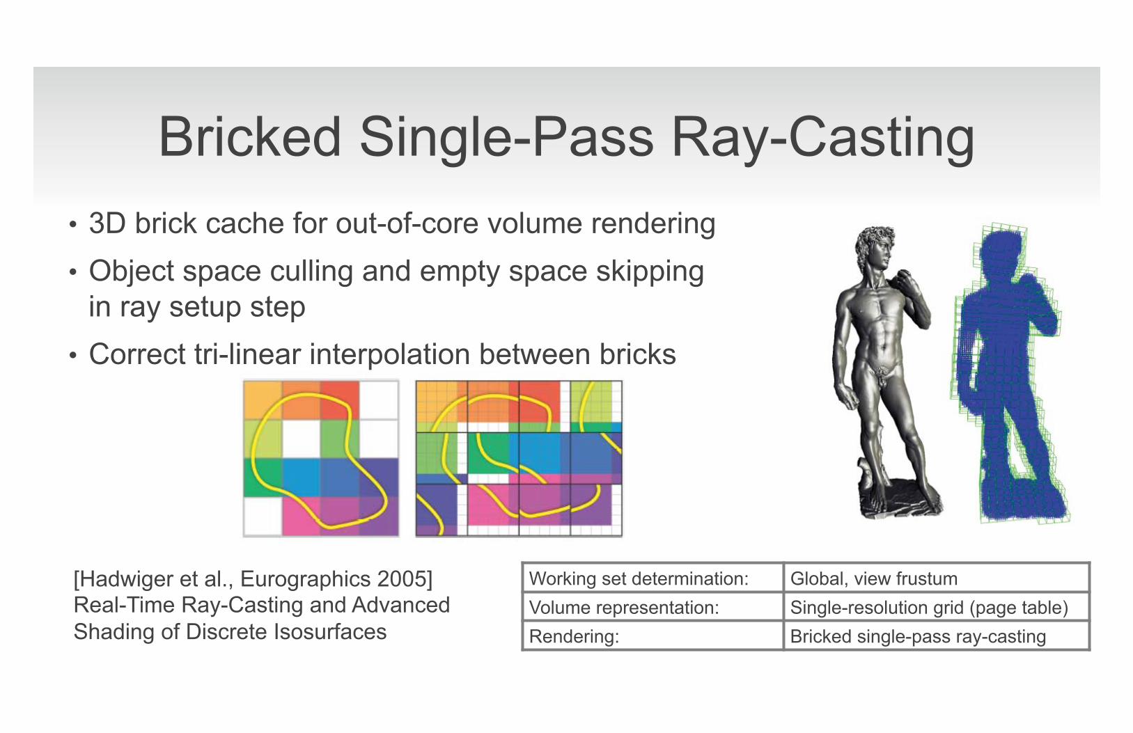
Bricked Single-Pass Ray-Casting •  3D brick cache for out-of-core volume rendering • Object space culling and empty space skipping

in ray setup step • Correct tri-linear interpolation between bricks

[Hadwiger et al., Eurographics 2005] Real-Time Ray-Casting and Advanced Shading of Discrete Isosurfaces

Working set determination: Global, view frustum Volume representation: Single-resolution grid (page table) Rendering: Bricked single-pass ray-casting

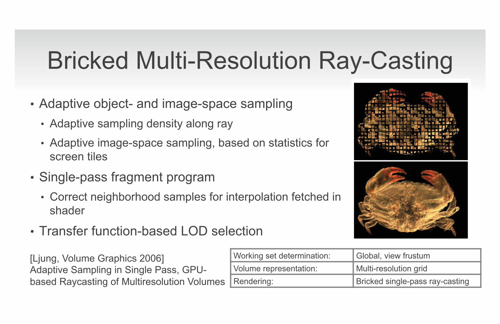
Bricked Multi-Resolution Ray-Casting • Adaptive object- and image-space sampling

•  Adaptive sampling density along ray

•  Adaptive image-space sampling, based on statistics for screen tiles

• Single-pass fragment program •  Correct neighborhood samples for interpolation fetched in

shader

• Transfer function-based LOD selection

[Ljung, Volume Graphics 2006] Adaptive Sampling in Single Pass, GPU-based Raycasting of Multiresolution Volumes

Working set determination: Global, view frustum Volume representation: Multi-resolution grid Rendering: Bricked single-pass ray-casting

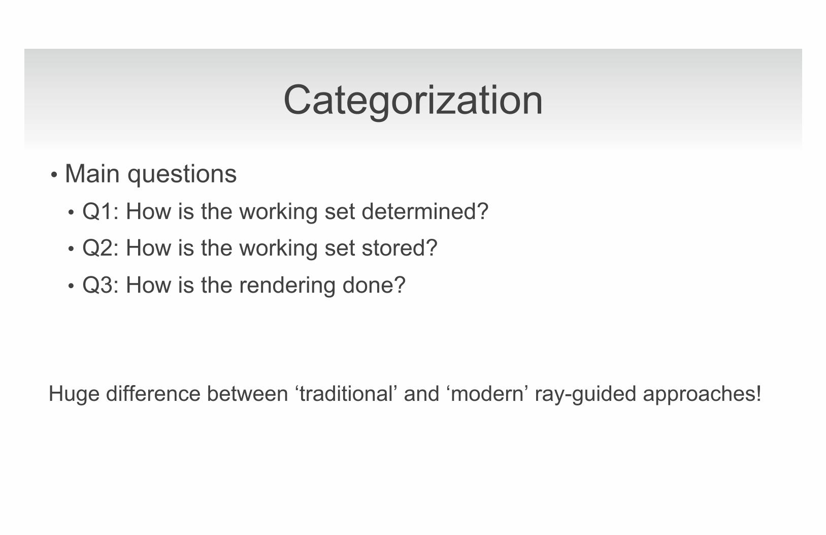
Categorization

• Main questions • Q1: How is the working set determined? • Q2: How is the working set stored? • Q3: How is the rendering done?

Huge difference between ‘traditional’ and ‘modern’ ray-guided approaches!

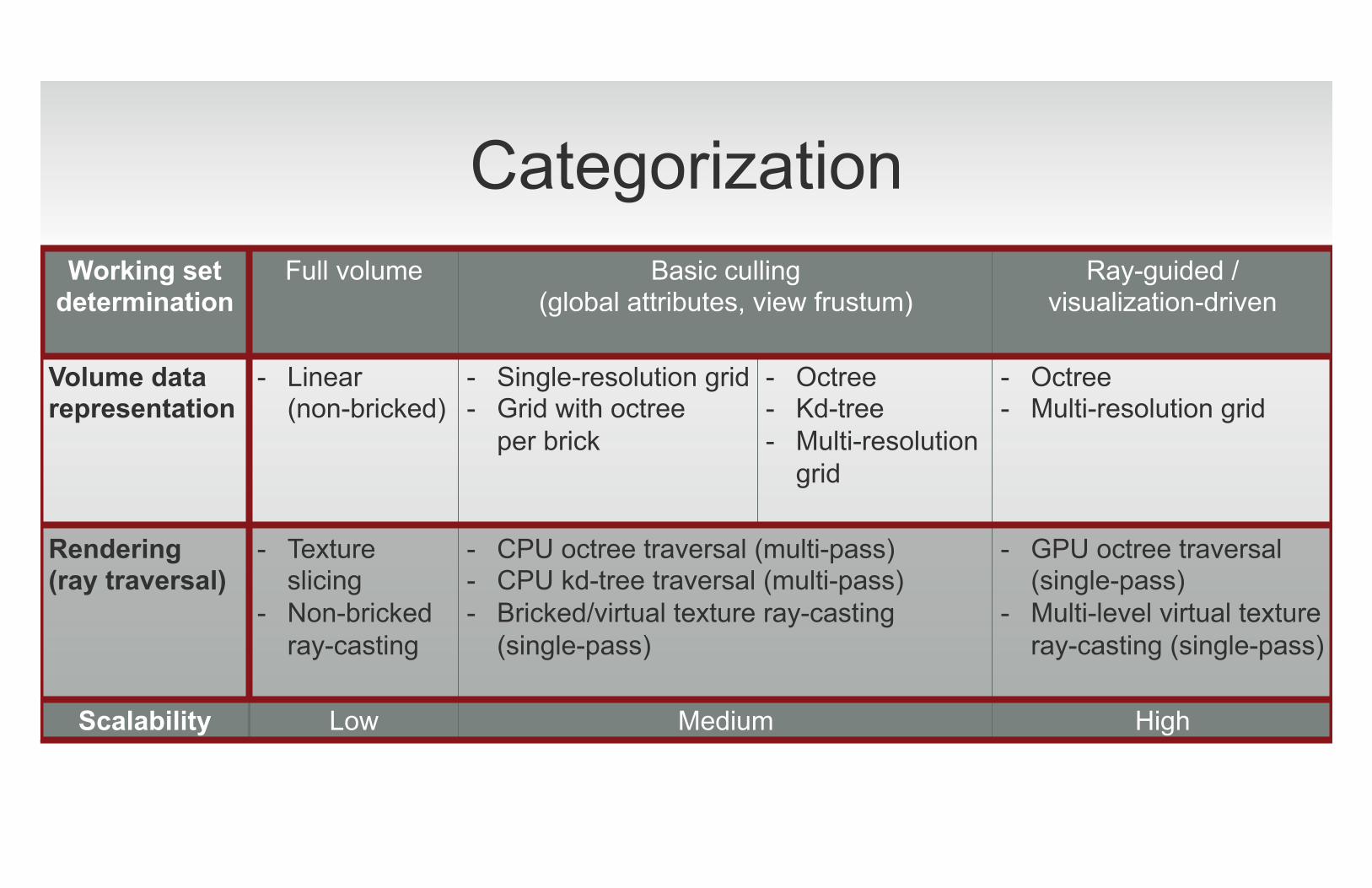
Categorization Working set

determination Full volume Basic culling

(global attributes, view frustum) Ray-guided /

visualization-driven

Volume data representation

-  Linear (non-bricked)

-  Single-resolution grid -  Grid with octree

per brick

-  Octree -  Kd-tree -  Multi-resolution

grid

-  Octree -  Multi-resolution grid

Rendering (ray traversal)

-  Texture slicing

-  Non-bricked ray-casting

-  CPU octree traversal (multi-pass) -  CPU kd-tree traversal (multi-pass) -  Bricked/virtual texture ray-casting

(single-pass)

-  GPU octree traversal (single-pass)

-  Multi-level virtual texture ray-casting (single-pass)

Scalability Low Medium High

Q1: Working Set Determination - Traditional

• Global attribute-based culling (view-independent) • Cull against transfer function, iso value, enabled objects, etc.

• View frustum culling (view-dependent) • Cull bricks outside the view frustum

• Occlusion culling?

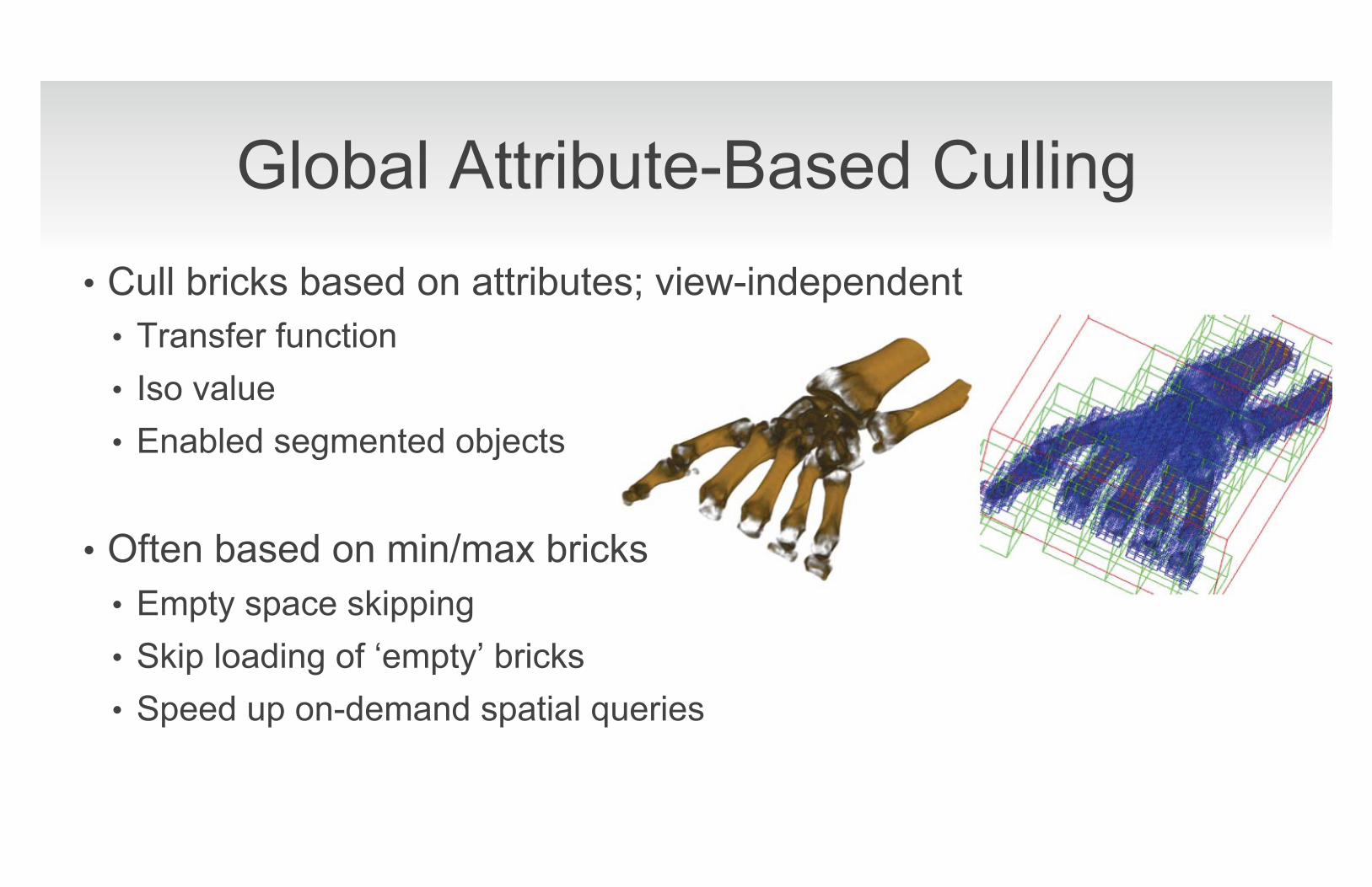
Global Attribute-Based Culling • Cull bricks based on attributes; view-independent

•  Transfer function •  Iso value •  Enabled segmented objects

• Often based on min/max bricks •  Empty space skipping •  Skip loading of ‘empty’ bricks •  Speed up on-demand spatial queries

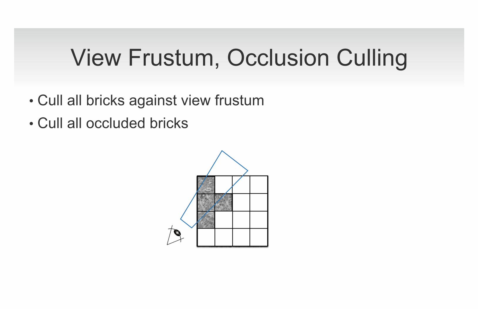
View Frustum, Occlusion Culling

• Cull all bricks against view frustum • Cull all occluded bricks

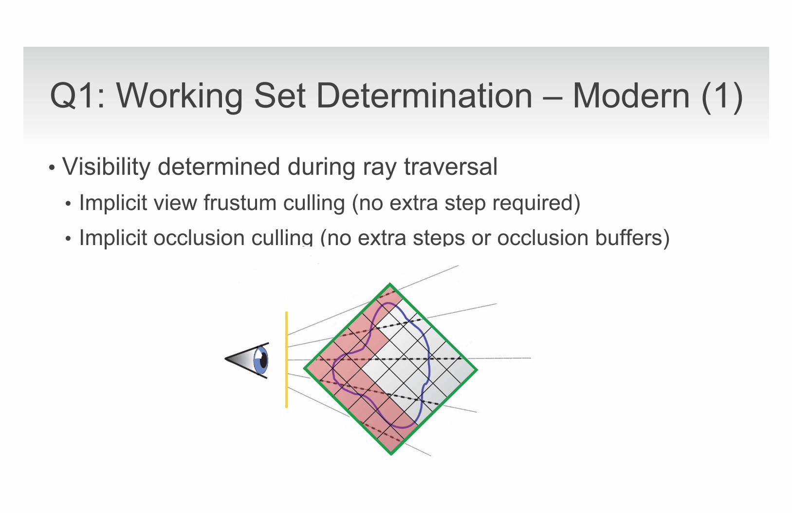
Q1: Working Set Determination – Modern (1)

• Visibility determined during ray traversal •  Implicit view frustum culling (no extra step required) •  Implicit occlusion culling (no extra steps or occlusion buffers)

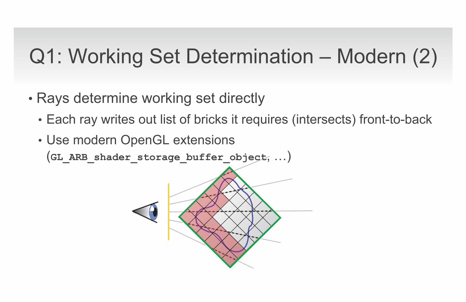
Q1: Working Set Determination – Modern (2)

• Rays determine working set directly • Each ray writes out list of bricks it requires (intersects) front-to-back • Use modern OpenGL extensions

(GL_ARB_shader_storage_buffer_object, �)

Q2: Working Set Storage - Traditional

• Different possibilities: •  Individual texture for each brick

•  OpenGL-managed 3D textures (paging done by OpenGL)

•  Pool of brick textures (paging done manually)

• Multiple bricks combined into single texture •  Need to adjust texture coordinates for each brick

Q2: Working Set Storage – Modern (1)

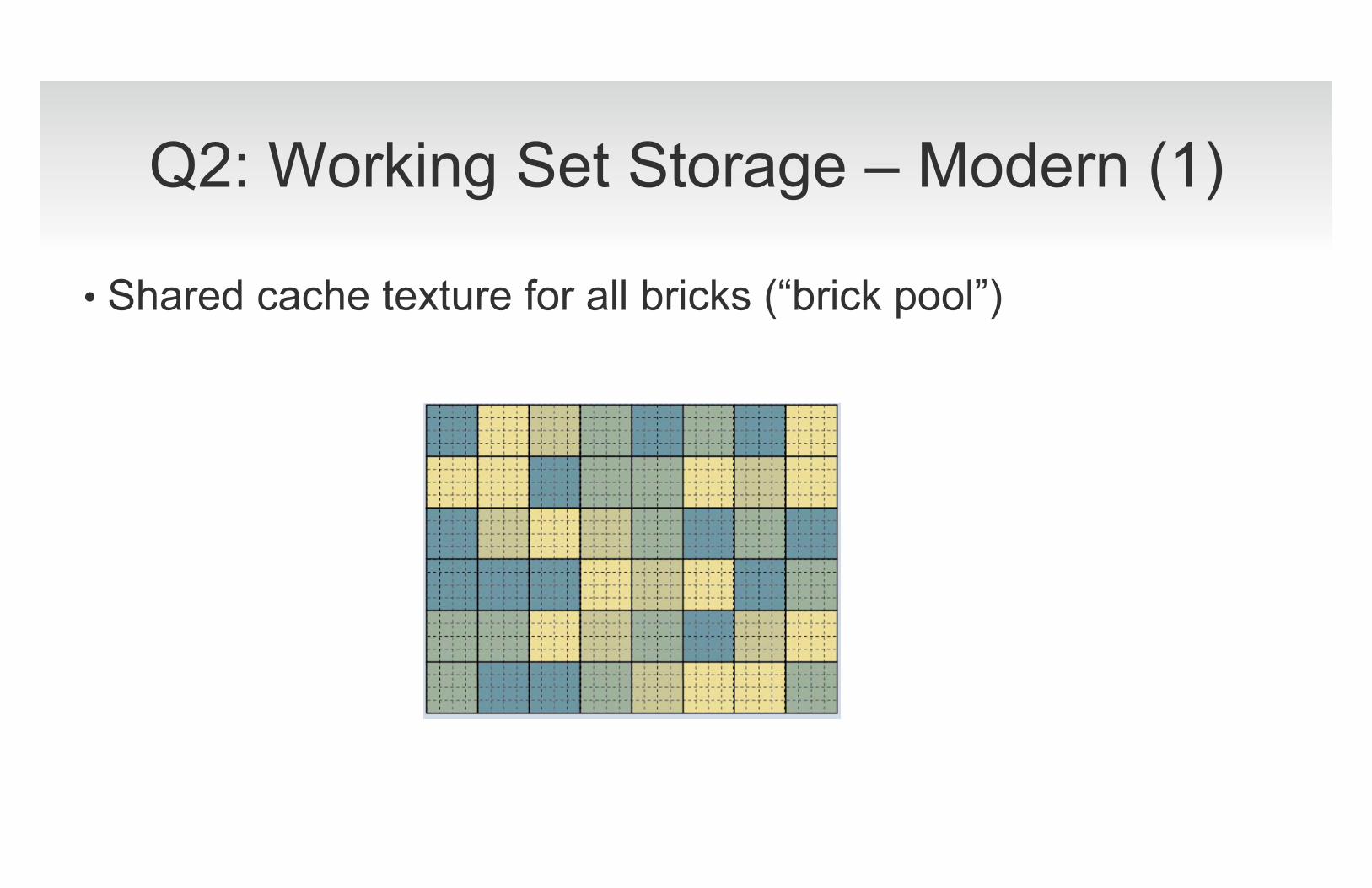
• Shared cache texture for all bricks (“brick pool”)

Q2: Working Set Storage – Modern (2)

• Caching Strategies • LRU, MRU

• Handling missing bricks • Skip or substitute lower resolution

• Strategies if the working set is too large • Switch from single-pass to multi-pass rendering •  Interrupt rendering on cache miss (“page fault handling”)

Q3: Rendering - Traditional

• Traverse bricks in front-to-back visibility order • Order determined on CPU • Easy to do for grids and trees (recursive)

• Render each brick individually • One rendering pass per brick

• Traditional problems • When to stop? (early ray termination vs. occlusion culling) • Occlusion culling of each brick usually too conservative

Q3: Rendering - Modern

• Preferably single-pass rendering • All rays traversed in front-to-back order • Rays perform dynamic address translation (virtual to physical) • Rays dynamically write out brick usage information

• Missing bricks (“cache misses”) • Bricks in use (for replacement strategy: LRU/MRU)

• Rays dynamically determine required resolution • Per-sample or per-brick

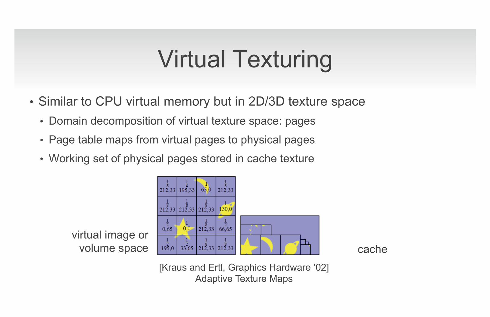
Virtual Texturing • Similar to CPU virtual memory but in 2D/3D texture space

•  Domain decomposition of virtual texture space: pages

•  Page table maps from virtual pages to physical pages

•  Working set of physical pages stored in cache texture

cache virtual image or

volume space

[Kraus and Ertl, Graphics Hardware ’02] Adaptive Texture Maps

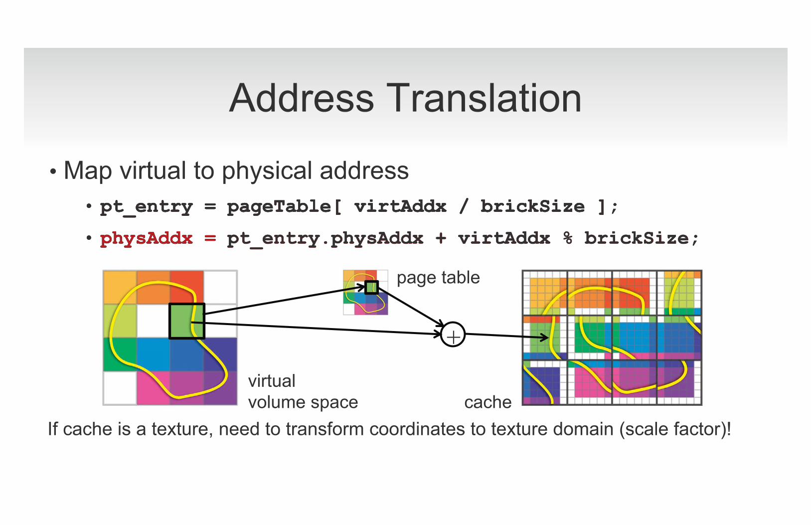
Address Translation

• Map virtual to physical address •  pt_entry = pageTable[ virtAddx / brickSize ];

•  physAddx = pt_entry.physAddx + virtAddx % brickSize;

If cache is a texture, need to transform coordinates to texture domain (scale factor)!

+��

•  virtAddx / brickSize •  pt_entry = pageTable[ virtAddx / brickSize ] •  pt_entry = pageTable[ virtAddx / brickSize ];

•  physAddx = pt_entry.physAddx + virtAddx % brickSize;

•  pt_entry = pageTable[ virtAddx / brickSize ];

•  physAddx = pt_entry.physAddx + virtAddx % brickSize;

•  pt_entry = pageTable[ virtAddx / brickSize ];

•  physAddx = pt_entry.physAddx + virtAddx % brickSize;

virtual volume space

cache

page table

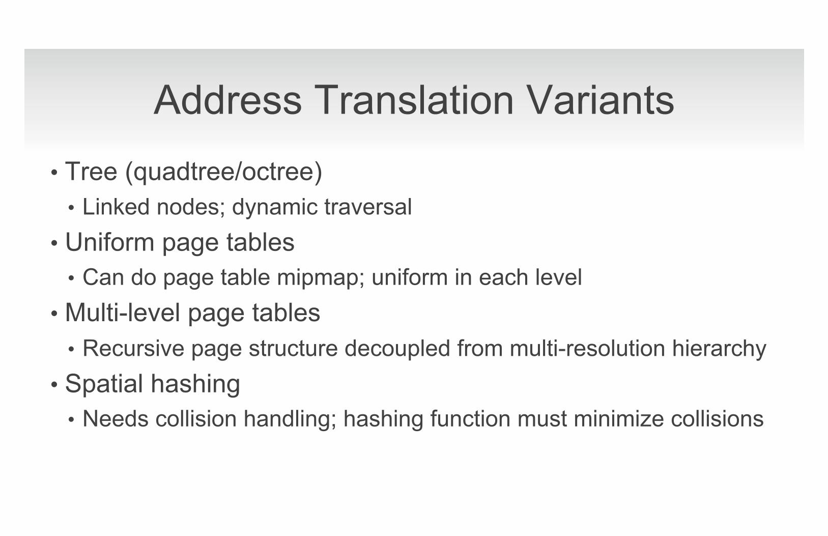
Address Translation Variants • Tree (quadtree/octree)

• Linked nodes; dynamic traversal • Uniform page tables

• Can do page table mipmap; uniform in each level • Multi-level page tables

• Recursive page structure decoupled from multi-resolution hierarchy • Spatial hashing

• Needs collision handling; hashing function must minimize collisions

Tree Traversal

• Adapt tree traversal from ray tracing • Standard traversal: recursive with stack • GPU algorithms without or with limited stack

•  Use “ropes” between nodes [Havran et al. ’98, Gobbetti et al. ‘08] •  kd-restart, kd-shortstack [Foley and Sugerman ‘05]

courtesy Foley and Sugerman

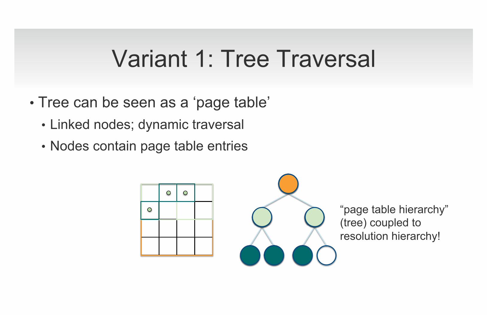
Variant 1: Tree Traversal

• Tree can be seen as a ‘page table’ • Linked nodes; dynamic traversal • Nodes contain page table entries

“page table hierarchy” (tree) coupled to resolution hierarchy!

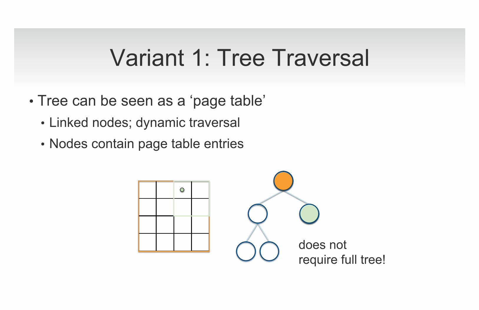
Variant 1: Tree Traversal

• Tree can be seen as a ‘page table’ • Linked nodes; dynamic traversal • Nodes contain page table entries

does not require full tree!

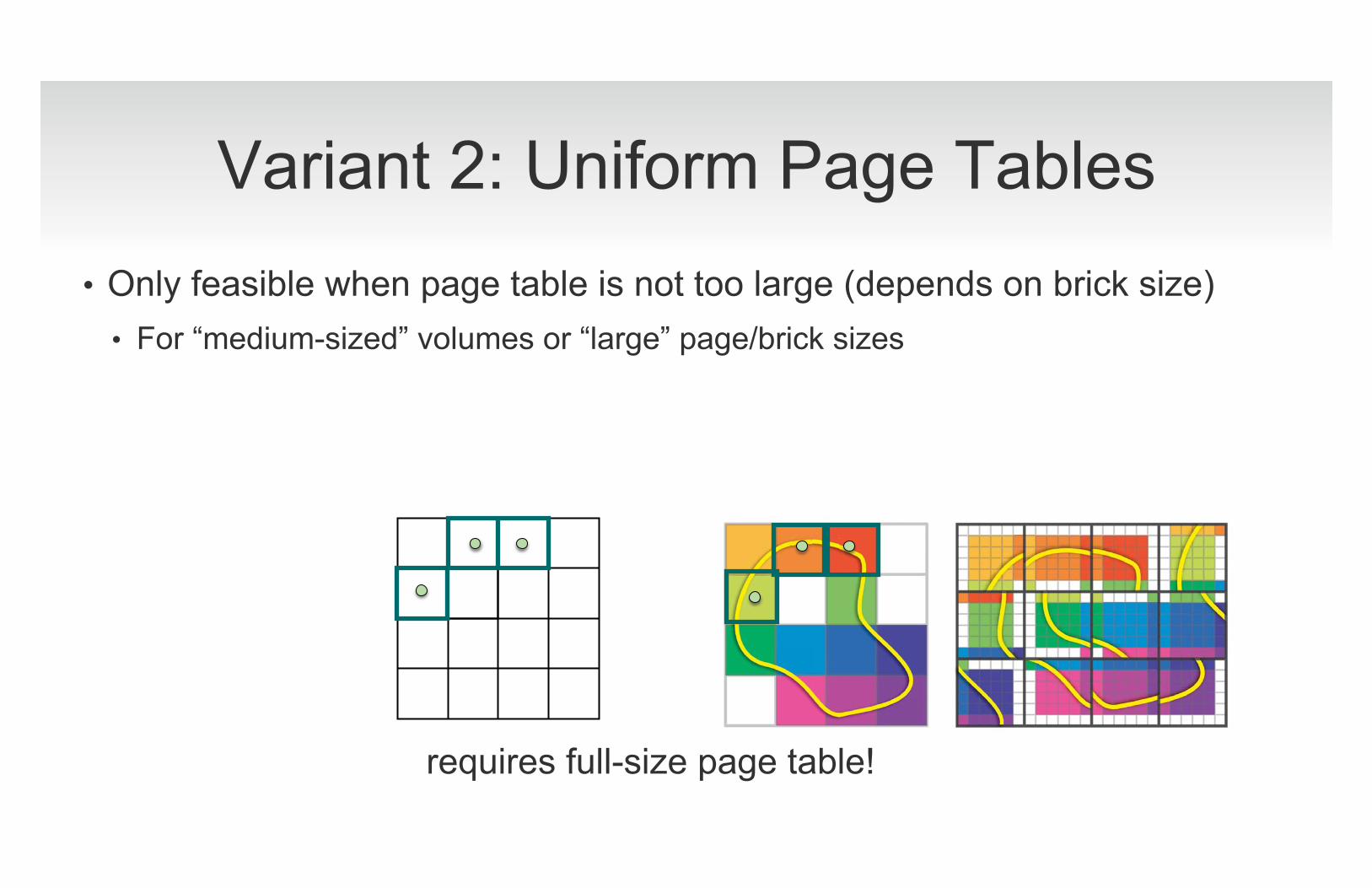
Variant 2: Uniform Page Tables • Only feasible when page table is not too large (depends on brick size)

•  For “medium-sized” volumes or “large” page/brick sizes

requires full-size page table!

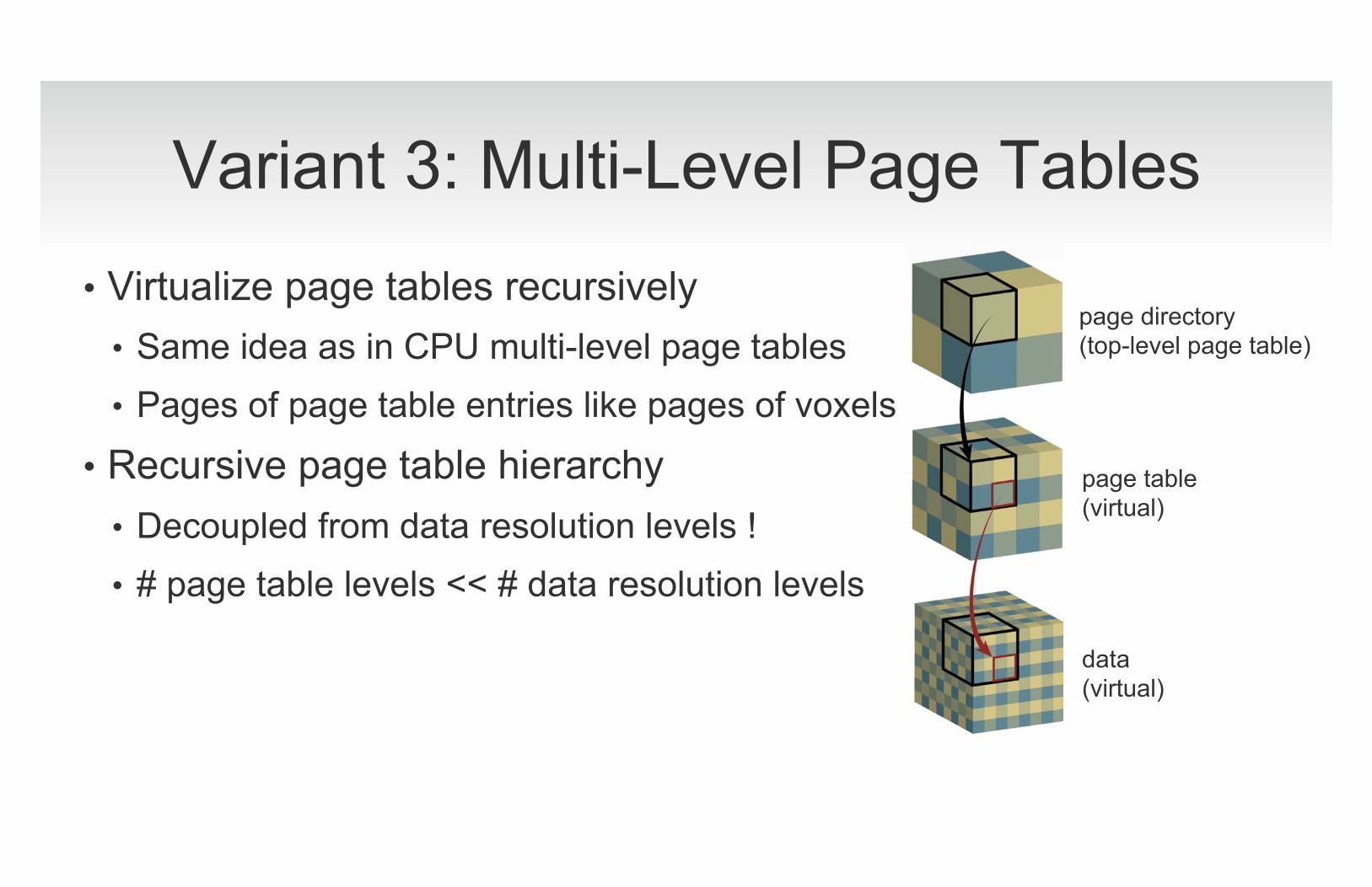
Variant 3: Multi-Level Page Tables • Virtualize page tables recursively

• Same idea as in CPU multi-level page tables • Pages of page table entries like pages of voxels

• Recursive page table hierarchy • Decoupled from data resolution levels ! •  # page table levels << # data resolution levels

data (virtual)

page table (virtual)

page directory (top-level page table)

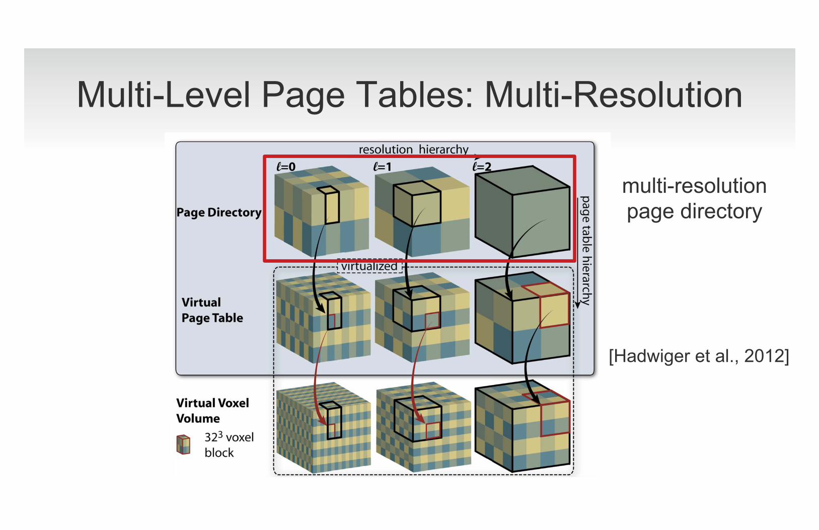
Multi-Level Page Tables: Multi-Resolution

multi-resolution page directory

[Hadwiger et al., 2012]

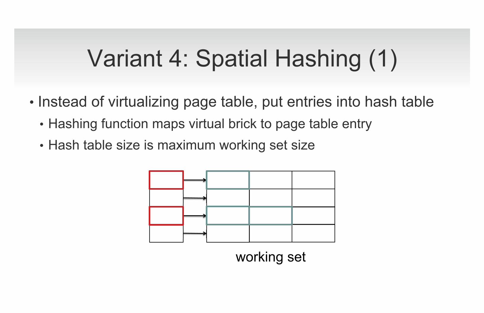
Variant 4: Spatial Hashing (1)

• Instead of virtualizing page table, put entries into hash table • Hashing function maps virtual brick to page table entry • Hash table size is maximum working set size

working set

Ray-guided Volume Rendering (1)

• Working set determination on GPU • Ray-guided / visualization-driven approaches

• Prefer single-pass rendering • Entire traversal on GPU • Use small brick sizes • Multi-pass only when working set too large for single pass

• Virtual texturing • Powerful paradigm with very good scalability

Ray-Guided Volume Rendering (2) • With octree traversal (kd-restart)

• Gigavoxels [Crassin et al., 2009]

•  Gigavoxel isosurface and volume rendering

•  Tera-CVR [Engel, 2011]

•  Teravoxel volume rendering with dynamic transfer functions

• Virtual texturing instead of tree traversal •  Petascale volume exploration of microscopy streams [Hadwiger et al., 2012]

•  Visualization-driven pipeline, including data construction

•  ImageVis3D [Fogal et al., 2013]

•  Analysis of different settings (brick size, �)

Examples

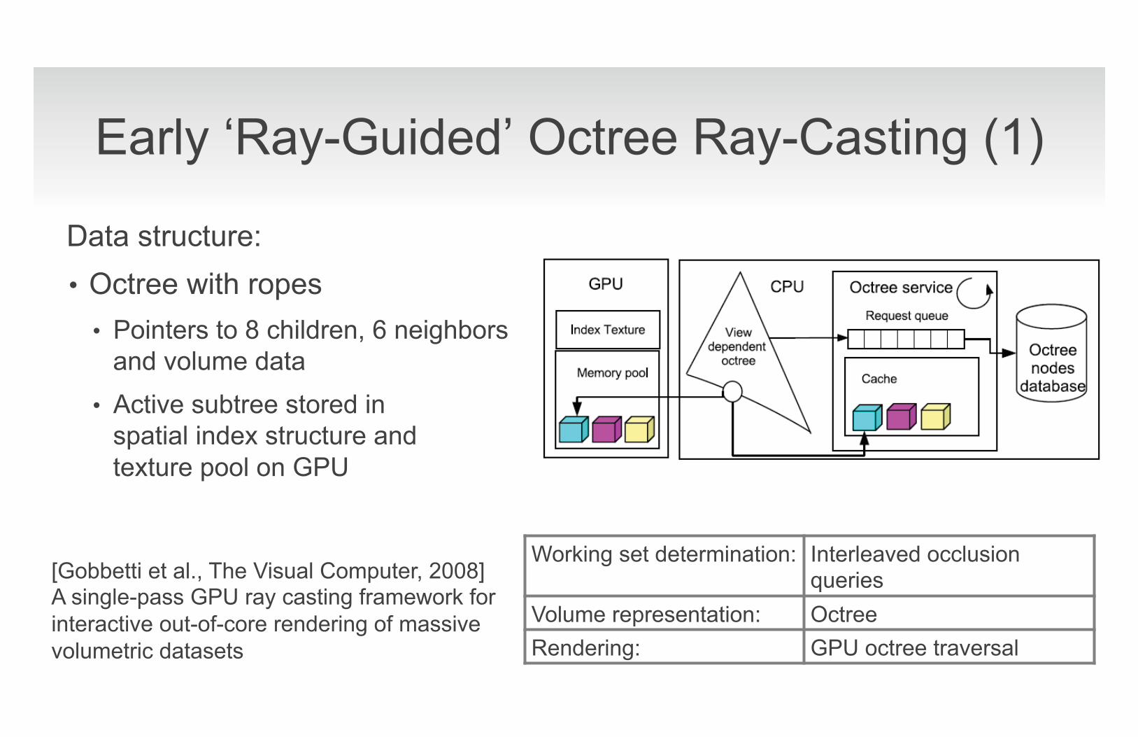
Early ‘Ray-Guided’ Octree Ray-Casting (1)

Data structure: • Octree with ropes

•  Pointers to 8 children, 6 neighbors and volume data

•  Active subtree stored in spatial index structure and texture pool on GPU

Working set determination: Interleaved occlusion queries

Volume representation: Octree Rendering: GPU octree traversal

[Gobbetti et al., The Visual Computer, 2008] A single-pass GPU ray casting framework for interactive out-of-core rendering of massive volumetric datasets

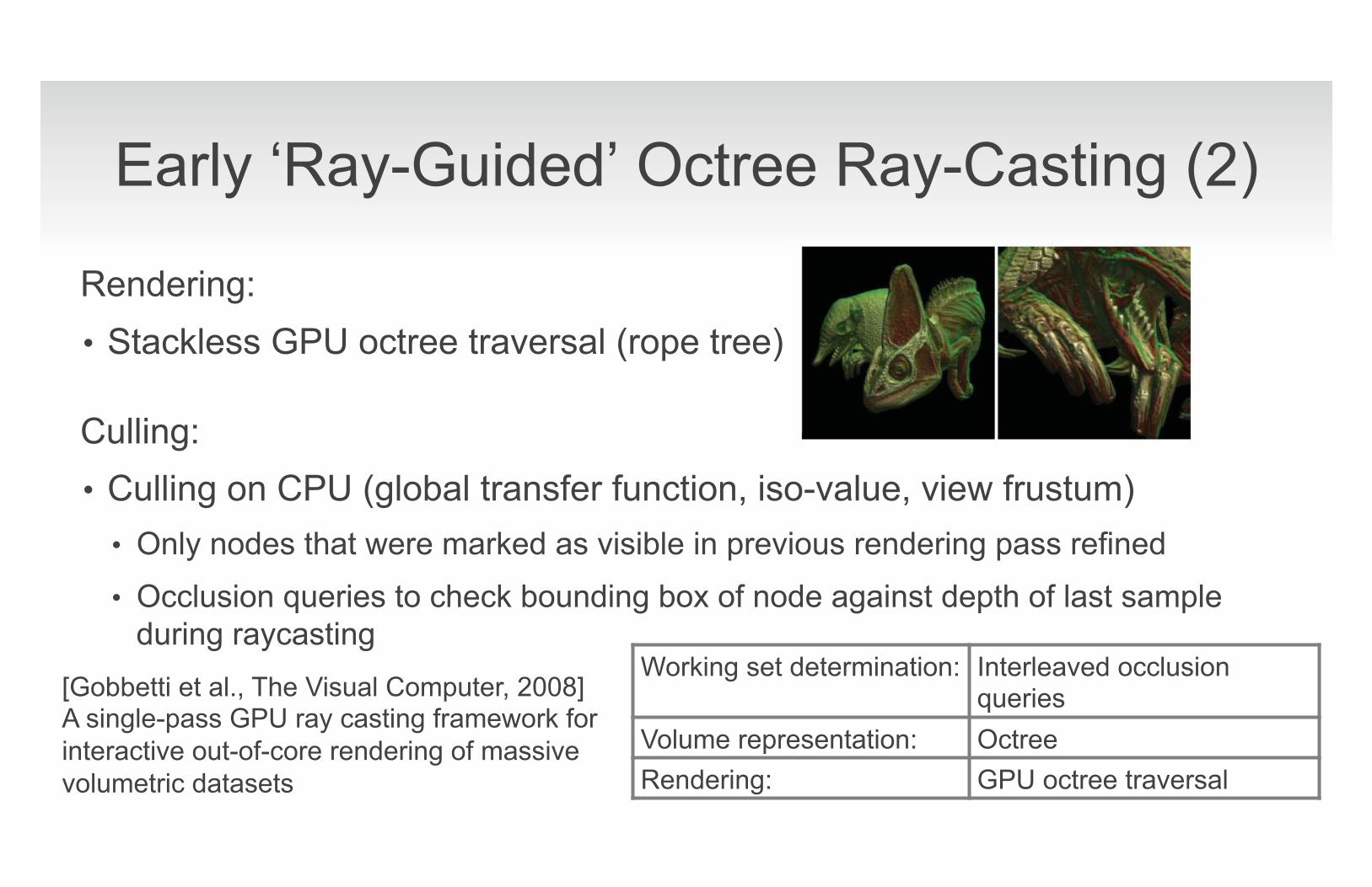
Early ‘Ray-Guided’ Octree Ray-Casting (2)

Rendering: • Stackless GPU octree traversal (rope tree)

Culling: • Culling on CPU (global transfer function, iso-value, view frustum)

•  Only nodes that were marked as visible in previous rendering pass refined

•  Occlusion queries to check bounding box of node against depth of last sample during raycasting

Working set determination: Interleaved occlusion queries

Volume representation: Octree Rendering: GPU octree traversal

[Gobbetti et al., The Visual Computer, 2008] A single-pass GPU ray casting framework for interactive out-of-core rendering of massive volumetric datasets

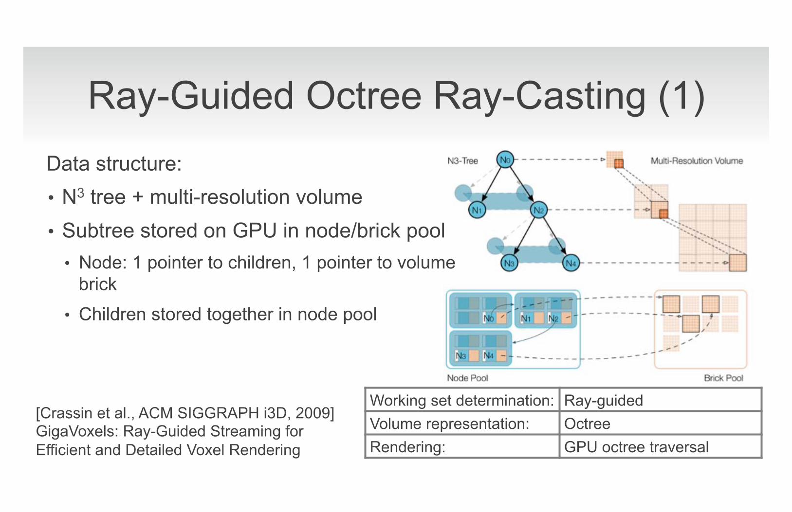
Ray-Guided Octree Ray-Casting (1) Data structure: • N3 tree + multi-resolution volume • Subtree stored on GPU in node/brick pool

•  Node: 1 pointer to children, 1 pointer to volume brick

•  Children stored together in node pool

Working set determination: Ray-guided Volume representation: Octree Rendering: GPU octree traversal

[Crassin et al., ACM SIGGRAPH i3D, 2009] GigaVoxels: Ray-Guided Streaming for Efficient and Detailed Voxel Rendering

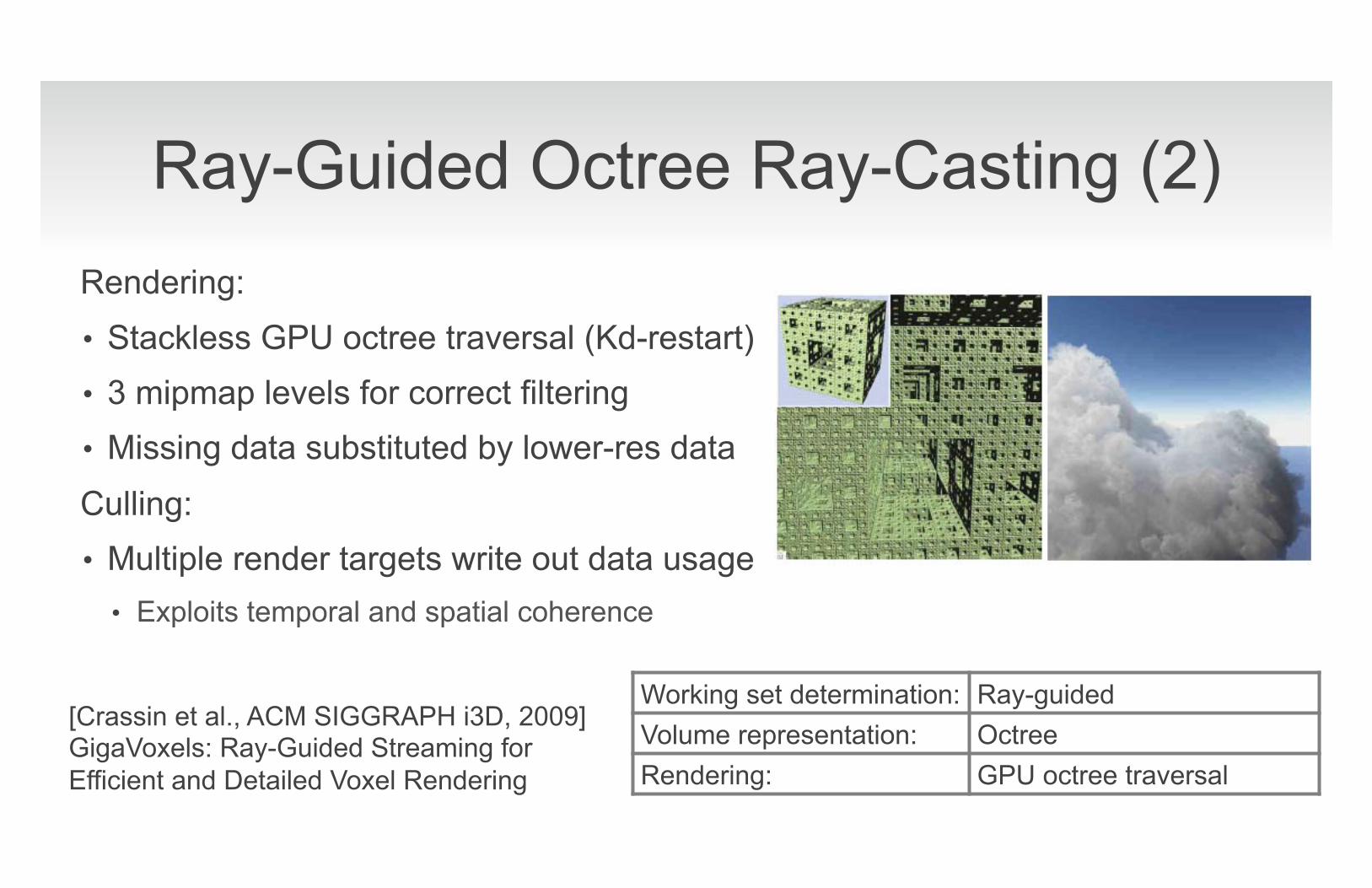
Ray-Guided Octree Ray-Casting (2) Rendering: •  Stackless GPU octree traversal (Kd-restart) •  3 mipmap levels for correct filtering •  Missing data substituted by lower-res data

Culling: •  Multiple render targets write out data usage

•  Exploits temporal and spatial coherence

Working set determination: Ray-guided Volume representation: Octree Rendering: GPU octree traversal

[Crassin et al., ACM SIGGRAPH i3D, 2009] GigaVoxels: Ray-Guided Streaming for Efficient and Detailed Voxel Rendering

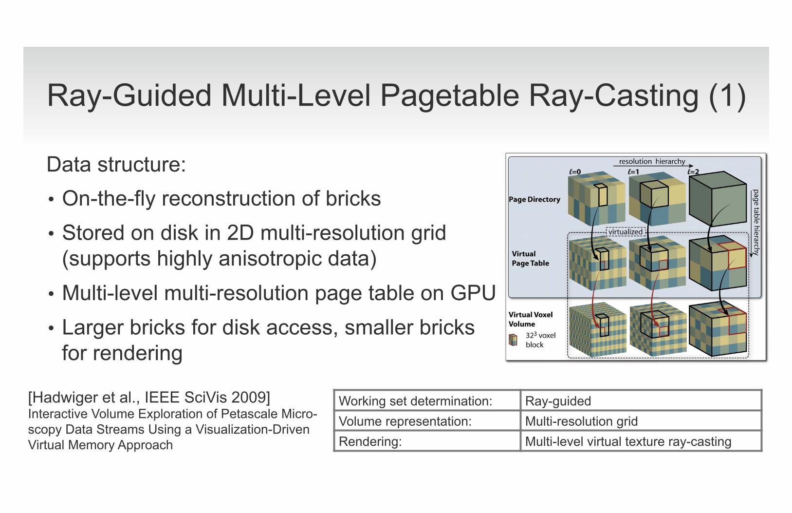
Ray-Guided Multi-Level Pagetable Ray-Casting (1)

Data structure: • On-the-fly reconstruction of bricks • Stored on disk in 2D multi-resolution grid

(supports highly anisotropic data) • Multi-level multi-resolution page table on GPU • Larger bricks for disk access, smaller bricks

for rendering

Working set determination: Ray-guided Volume representation: Multi-resolution grid Rendering: Multi-level virtual texture ray-casting

[Hadwiger et al., IEEE SciVis 2009] Interactive Volume Exploration of Petascale Micro- scopy Data Streams Using a Visualization-Driven Virtual Memory Approach

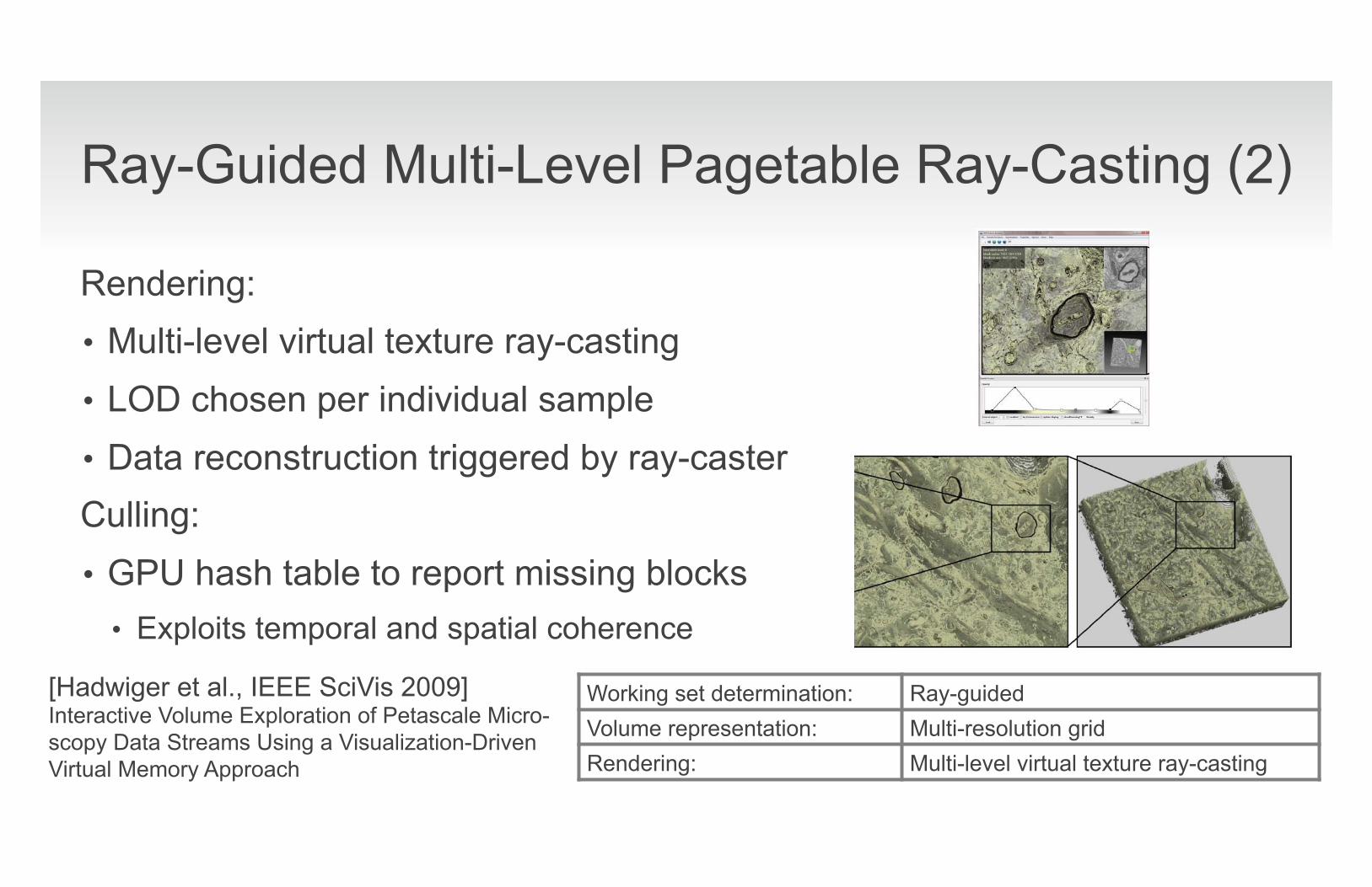
Ray-Guided Multi-Level Pagetable Ray-Casting (2)

Rendering: • Multi-level virtual texture ray-casting •  LOD chosen per individual sample • Data reconstruction triggered by ray-caster Culling: • GPU hash table to report missing blocks

•  Exploits temporal and spatial coherence

Working set determination: Ray-guided Volume representation: Multi-resolution grid Rendering: Multi-level virtual texture ray-casting

[Hadwiger et al., IEEE SciVis 2009] Interactive Volume Exploration of Petascale Micro- scopy Data Streams Using a Visualization-Driven Virtual Memory Approach

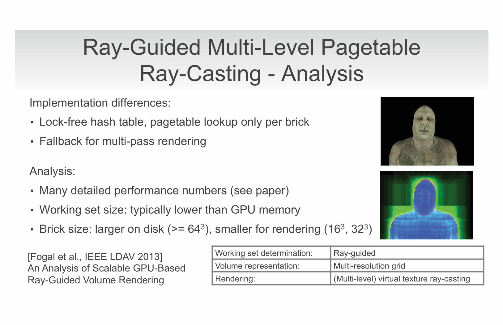
Ray-Guided Multi-Level Pagetable Ray-Casting - Analysis

Implementation differences: •  Lock-free hash table, pagetable lookup only per brick

•  Fallback for multi-pass rendering

Analysis:

•  Many detailed performance numbers (see paper)

•  Working set size: typically lower than GPU memory

•  Brick size: larger on disk (>= 643), smaller for rendering (163, 323)

Working set determination: Ray-guided Volume representation: Multi-resolution grid Rendering: (Multi-level) virtual texture ray-casting

[Fogal et al., IEEE LDAV 2013] An Analysis of Scalable GPU-Based Ray-Guided Volume Rendering

Conclusion

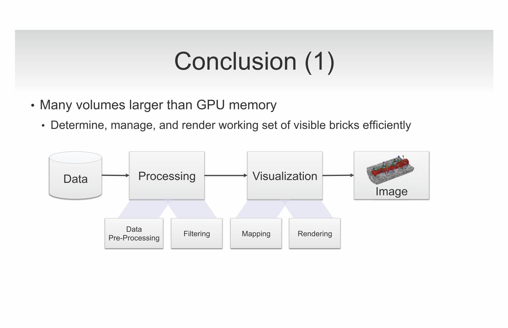
Conclusion (1) • Many volumes larger than GPU memory

•  Determine, manage, and render working set of visible bricks efficiently

Data Processing Visualization

Image

Filtering Data Pre-Processing Mapping Rendering

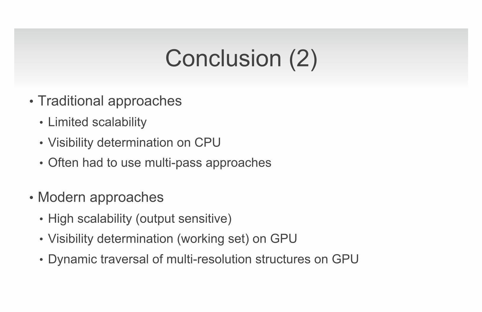
Conclusion (2) • Traditional approaches

•  Limited scalability • Visibility determination on CPU • Often had to use multi-pass approaches

• Modern approaches • High scalability (output sensitive) • Visibility determination (working set) on GPU • Dynamic traversal of multi-resolution structures on GPU

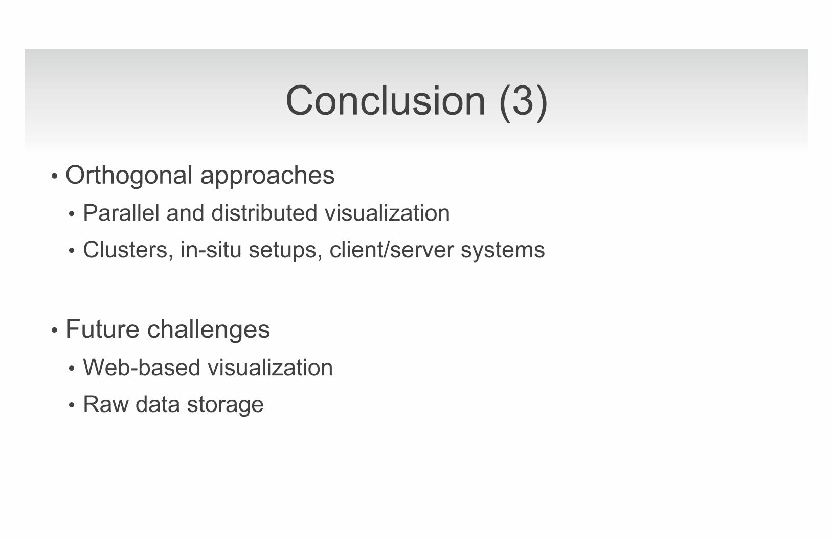
Conclusion (3)

• Orthogonal approaches • Parallel and distributed visualization • Clusters, in-situ setups, client/server systems

• Future challenges • Web-based visualization • Raw data storage

THANKS�

Webpage:�http://people.seas.harvard.edu/~jbeyer/star.html�