ISBN 0 902246 99 2

© J. Silk

ANALYSIS OF COVARIANCEAND COMPARISON OF REGRESSION LINES

J. Silk

CATMOG

(Concepts and Techniques in Modern Geography)

CATMOG has been created to fill a teaching need in the field of quantitativemethods in undergraduate geography courses. These texts are admirable guidesfor the teachers, yet cheap enough for student purchase as the basis of class-work. Each book is written by an author currently working with the techniqueor concept he describes.

1. An introduction to Markov chain analysis - L. Collins

2. Distance decay in spatial interactions - P.J. Taylor

3. Understanding canonical correlation analysis - D. Clark

4. Some theoretical and applied aspects of spatial interactionshopping models - S. Openshaw

5. An introduction to trend surface analysis - D. Unwin

6. Classification in geography - R.J. Johnston

7. An introduction to factor analytical techniques - J.B. Goddard & A. Kirby

8. Principal components analysis - S. Daultrey

9. Causal inferences from dichotomous variables - N. Davidson

10. Introduction to the use of logit models in geography - N. Wrigley

11. Linear programming: elementary geographical applications of thetransportation problem - A. Hay

12. An introduction to quadrat analysis - R.W. Thomas

13. An introduction to time-geography - N.J. Thrift

14. An introduction to graph theoretical methods in geography - K.J. Tinkler

15. Linear regression in geography - R. Ferguson

16. Probability surface mapping. An introduction with examples andFortran programs - N. Wrigley

17. Sampling methods for geographical research - C. Dixon & B. Leach

18. Questionnaires and interviews in geographical research -C. Dixon & B. Leach

19. Analysis of frequency distributions - V. Gardiner & G. Gardiner

20. Analysis of covariance and comparison of regression lines - J. Silk

21. An introduction to the use of simultaneous-equation regression analysisin geography - D. Todd

Other titles in preparation

This series, Concepts and Techniques in Modern Geography is produced by the Study Group in Quantitative Methods, ofthe Institute of British Geographers.For details of membership of the Study Group, write to theInstitute of British Geographers,) Kensington Gore, London, S.W.7.The series is published by Geo Abstracts, University of East Anglia,Norwich, NR4 7TJ, to whom all other enquiries should be addressed.

CONCEPTS AND TECHNIQUES IN MODERN GEOGRAPHY No. 20

ANALYSIS OF COVARIANCE AND COMPARISON OF REGRESSION LINES

by

John Silk

(University of Reading)

CONTENTS

I INTRODUCTION

(i) Prerequisites 3

(ii) Purpose 4

II THE ANALYSIS OF VARIANCE AND LINEAR REGRESSION MODELS

(i) The analysis of variance model 6

(ii) The linear regression model 8

III SPECIFICATION OF MODELS FOR DUMMY VARIABLE ANALYSIS

(i) Informal description of models 11

(ii) Formal specification of models in dummy variableanalysis 13

IV STATISTICAL COMPARISON OF MODELS

(i) Comparisons 'between' models 18

(ii) Sequence of comparisons 19

(iii) Comparisons involving the full model 20

(iv) Comparisons 'within' models 20

V COMPARISONS IN THE ANALYSIS OF COVARIANCE-A WORKED EXAMPLE

(i) A conventional approach 21

(ii) Approach based on dummy variable analysis 27

(iii) Checking assumptions underlying the analysisof covariance 30

VI COMPARISON OF REGRESSION LINES BY DUMMY VARIABLE ANALYSIS -A PRACTICAL APPLICATION: STOCKING AND ELWELL (1976)

(i) Introduction 31

(ii) Results 34

VI EXAMPLES OF ANALYSIS OF COVARIANCE AND DUMMY VARIABLEANALYSIS IN GEOGRAPHY 40

VII COMPUTER ROUTINES 42

VIII FURTHER EXTENSIONS AND CONCLUSION 43

BIBLIOGRAPHY 44

ACKNOWLEDGEMENTS

To Sarah Morgan for typing the text, Sheila Dance and Brian Rogersfor drawing the diagrams, and Philip Brice for photographicreduction work.

We also wish to thank the following for permission to reproducecopyright material:

The editor of Geografiska Annaler, Series A, for figures 3 and4 from The Thickness of the active layer on some of Canada'sarctic slopes.' F.G. HANNELL, Geografiska Annaler, 55A,1973, p 181 (Fig.2, p 6); andThe Institute of British Geographers for figures 7, 8 and 9 from'Rainfall erosivity over Rhodesia.' M.A. STOCKING & H.A. ELWELL,Transactions, 1(2), 1976 (Figs. 9, p 32; 10, p 36; 11, p 39).

INTRODUCTION

The analysis of covariance brings together features of both theanalysis of variance and regression analysis, and is closely allied withtechniques for the comparison of regression lines.

Two topics will be discussed in this introduction. As a prerequisite,we outline the general features of the analysis of variance and regressionanalysis, considering particularly the levels of measurement associatedwith each. Then, we consider the purposes for which the analysis ofcovariance and comparisons of regression lines may be used.

(i) Prerequisites

Classically, the analysis of variance is concerned with the estimationand comparison of the mean values of a response or dependent variableunder different conditions. Each 'condition' is represented by a class orcategory in the analysis. Because we may regard the value of any givenobservation of the response variable as (at least in part) dependent upon/the category or class in which it falls, the categories themselves may beregarded as 'values' or 'levels' of an independent or explanatory variable.

Such 'values' are said to be measured on a nominal scale if thereis no intrinsic ordering of the categories. This might be the case ifthe explanatory variable were aspect, as represented by the categories'north-facing' and 'south-facing', or region, as represented by a number ofphysiographic zones or administrative districts. An intrinsic orderingof the categories, as in the case of socio-economic status, age or incomegroups, is said to represent measurement on an ordinal scale. For example,census volumes present much information according to the eight age groups0 - 4, 5 - 14, ...... 55 - 64, 65 or over. If these groups are numbered

1 to 8 respectively, then the numbers may be taken to represent theranking or ordering of the groups. Thus, the 'values' or 'levels' of acategorical explanatory variable may represent ordered or unorderedcategories.

Regression analysis concerns itself with the relationship between adependent or response variable and one or more independent or explanatoryvariables. Conventionally, the assumption is made that all variables,whether dependent or independent, are measurable on an interval or ratioscale. Both scales allow us to determine the distance along the scalebetween the attributes of any two individuals or events, as well as theirrank order. Measurement based on a ratio scale is taken to be at a higherlevel than that based on an interval scale, because the former providesmeasurements that can be referred to a natural origin or absolute zeropoint, whereas the latter cannot. The Fahrenheit and Centigrade temperaturescales are examples of interval scales. A reading of 0

°Centigrade corres-

ponds to 32°F, and of 0

°Fahrenheit to -17.8

° Centigrade, showing that the

zero points are arbitrarily determined in each case. Many of the variablesused in geographical research are measurable on a ratio scale, for exampledistance, altitude, population and income.

3

In addition, it is usually assumed that the response or dependentvariable is continuous (i.e. it can assume an unlimited number of inter-mediate values), and that the same holds for all independent or explanatoryvariables measured on an interval or ratio scale.

The case in which the dependent or response variable is categorizedis not discussed here, but a detailed treatment may be found in anothermonograph in the CATMOG series (Wrigley, 1976). A technique such as theanalysis of covariance, therefore, which combines features of the analysisof variance and regression analysis, is concerned with a response ordependent variable, measured on an interval or ratio scale, and a set ofexplanatory variables, of which some may be measurable on an interval orratio scale, and others on a nominal or ordinal scale.

Familiarity with the one-way analysis of variance model, assumingfixed-effects, and with the theory underlying regression analysis, isessential, and brief reviews of both kinds of model are provided in SectionII of this monograph. Many of the concepts and principles involved havealso been discussed by Unwin (1975) and Ferguson (1978) in earliercontributions to the CATMOG series.

(ii) Purpose

The techniques described in this paper enable the investigator to:

1) Introduce an additional independent variable, measured on a ratioor interval scale, to adjust mean values already estimated accordingto the analysis of variance model.

2) Compare two or more bivariate regression lines, assuming that thevariables included in the regression model are the same in each case.

The value of the procedure described in 1) becomes apparent if we brieflyconsider a hypothetical example (to be studied in detail in Section V).Suppose that a study is carried out to establish whether travel behaviourof the elderly differs from that of the rest of the population in a parti-cular city. Information is obtained by stratifying households into elderlyand non-elderly groups, randomly selecting a number of households from eachgroup, and asking a member of each household to keep a record of all house-hold daily travel behaviour for four weeks. One crude index of travel be-haviour is the average number of visits made per week to the city centre,

city centre, X, we may find that elderly households tend to live furtheraway from the city centre, on average, than non-elderly households.Assuming that trip rates decline with distance, it could well be that theelderly households make fewer trips not because they are old and instrinsi-cally less mobile, but because they happen to live slightly further awayfrom the city centre than do households in other groups. It is desirable toisolate the influence of distance so that the difference between the two

amounts. Under certain conditions, described in Section V, such adjustmentsmay be made using the analysis of covariance.

4

Figure 1. Hypothesized relationships between cognitive distance (Y) andobjective road distance (X) (redrawn from Briggs, 1973).

The above provides an example of confounding, in which the influencesof two or more variables on some phenomenon are difficult, or sometimesimpossible, to disentangle. In this case one variable is categorical(elderly or non-elderly) and the other measurable on a ratio scale in termsof distance.

A number of reasons may be put forward for comparing regression lines:

a) To test a priori hypotheses. For instance, Briggs (1973) reasonedthat distance estimates made by students would be more exaggeratedin the direction of the town centre than away from it, and alongroutes involving bends than routes that did not. The rankingsof the slope terms with respect to the four cases are illustratedin Figure 1.

b) As an aid to parsimonious description and explanation. It maybe found that the values taken on by the slope terms of a numberof regression lines are not significantly different. This maywell be the case in Figure 2, which shows separate regressionlines for north-and south-facing Arctic slopes of thickness ofthe active layer (Y) on daily radiation total (X) (Hannell, 1973).If it is found that the two slopes do not differ significantly,then the initial model based on two slopes and two intercepts maybe reduced to another based on one slope and two intercepts.Opportunities for simplification are particularly evident if, say,a study of the relationship between two variables X and Y isconducted in ten different regions.

c) To obtain better estimates. This characteristic may be associatedwith the simplification process described above. A slope term of aregression relationship, for instance, may be estimated moreaccurately from two sets of observations than from one.

If we are not particularly interested in the precise form of therelationship between two or more variables, or in estimation problems ingeneral, the various influences may be 'sorted out' with the aid of ananalysis based on partial correlation coefficients (Weatherburn, 1962,256-257; Blalock, 1964; Taylor 1969). Discussion of methods for explicitly

5

Figure 3. The analysis of variance model a) Parameters b) Estimates.

7

Figure 2. Relationship between thickness of the active layer (Y) and dailyradiation total (X) on north- and south-facing slopes (adaptedfrom Hannell, 1973).

controlling for the influence of a third variable may be found in Davidson(1976) and Ferguson (1978).

II THE ANALYSIS OF VARIANCE AND LINEAR REGRESSION MODELS

(i) The analysis of variance model

Suppose we are interested in the mean values of a response variable,Y, in three different regions represented by the categorical explanatoryvariable, A. Let the true mean values of Y for each region be represented

Certain assumptions are made about the behaviour of the terms onthe right hand side of (3):

Rearrangement of (1), and study of Figure 3(a) shows that we may expresseach regional mean as a deviation from the overall mean:

6

Table 1. Least squares estimators for the analysis of variance model

Population parameter Estimator

Overall sample mean

Group or regional samplemean

Estimated effect of beingin ith region or group

Formula Description

Error or disturbance term

= regional or group membership

= number of sample observations in region or group i

= position of observation within region or group

9

Sample residual

Provided these assumptions are fulfilled, at least approximately, theleast squares estimators of the population parameters have highly desirableproperties, being unbiased and of minimum variance (Unwin, 1975, 19-20)(Table 1). The estimates themselves i.e. the actual numerical values yieldedby applying the estimators in any particular investigation, will not gener-ally equal the values of the unknown population parameters. This means that

The investigator may wish to test certain hypotheses relating to theparameters, and approximate fulfillment of assumptions 3, 4 and 5 ensuresthat tests of significance based on the t and F distributions may be employed.

ii) The linear regression model

As for the analysis of variance model, we are interested in estimatingthe values of a response or dependent variable, Y. This time, however, weassume that changes in the values of some non-categorical explanatoryvariable, X, measured on an interval or ratio scale, cause or produce achange in the values of Y. If the assumption of causality seems too strongor inappropriate, we may instead speak in terms of changes in the value ofY which are associated with changes in the value of X.

The relationship between the two variables - only the bivariate caseis considered here - is assumed to be linear, and may be expressed:

showing the values of Y corresponding to all possible values of X withinthe range covered by the abscissa in the diagram, is represented by thesolid line in Figure 4.

Apart from that of linearity, many of the assumptions underlyingregression analysis are similar to those already made with respect to theanalysis of variance: fixed population values of the intercept and slopeterms, and of the values of X (the latter should also be measured with

about the regression line for all values of X.

Estimates of the population parameters are obtained from the sampleobservations using the least-squares estimators from Table 2 in the equation:

8

Table 2. Least squares estimators for the bivariate linear regression model

Population parameter Estimator

Formula Description

Error or disturbance term

Sample residual

Assumptions regarding the population disturbance term are based onthe notion that any of a range of individual values of Y may be associatedwith a given value of X, so that the population regression line may beregarded as the locus of the mean values of Y corresponding to all possible

intermediate values of X within a given range. This view furtheremphasises the similarity with the analysis of variance model, i.e. estimat-ion of mean values, and makes the adjustment of mean values based onregression techniques seem more 'natural' when the procedure is carried out.

are to be constructed about the regression line Draper & Smith, 1966, 21-24.)

The form of the analysis of covariance model is given in Figure 5(b),and shows the influence of a categorical variable A, because there is aregression line for each of three (hypothetical) categories, combined withthat of the continuous explanatory variable X. Apart from those alreadyoutlined, additional assumptions of the analysis of covariance model are

1) The regression lines for each category must be of equal slope orparallel.

2) The population disturbance terms for the observations in eachcategory should show equal variance about each of the parallelregression lines.

3) Differences between the mean values of the covariate, X, foreach category of the categorical variable A, should be 'relatively

small'.

The implications of these assumptions will become clear as the discussionproceeds.

III SPECIFICATION OF MODELS FOR DUMMY VARIABLE ANALYSIS

i) Informal description of models

Before formally specifying models, it is helpful to describe thelinks between the analysis of variance (ANOVA), the analysis of covariance(ANCOVA), and the general process of comparing regression lines.

Consider the horizontal lines representing the means of the dependentvariable Y for each of three sets of observations in Figure 5(a). Thispattern of observations is one for which the three means may be comparedusing ANOVA. Notice that ANOVA may be regarded as analysis of values ofa dependent variable, ignoring association with variables other than thosewhose influence may be summarised by grouping the observations. In Figure5(a), the 'ignored variable' is X.

The residual deviations of the observations about their respectivemeans may be scrutinised in the same way as residuals about regression(Ferguson, 1978, 14-15). We are particularly concerned with the case inwhich a trend within the residuals is suspected when plotted against somecontinuous independent variable or covariate, X. Figure 5(a) clearlyshows such a trend for the observations within each group.

The simplest model incorporating a covariate is the analysis of cov-ariance (ANCOVA) model, which assumes the same slope within each of the threesets of residuals (Figure 5(b)). Notice that the intercept terms of theregression lines are permitted to vary between groups, but not their slopes.In this paper, the ANCOVA model will also be known as the Parallel model,

Figure 4. The linear regressionmodel - parameters and estimates

Sample estimate ofslope term

Sample estimate ofintercept term

Sample estimate of(mean) value of Ycorresponding to X i

10 11

12

as it represents one of four basic types of regression model which may befitted to a set of observations. The Intercept model allows slopes to varybut not intercepts (Figure 5(e)) and the Full model leaves both slopesand intercepts unconstrained so yielding three separate regression lines asin Figure 5(c). If the classification of observations is thought to betotally irrelevant i.e. the categorical variable A is deleted, then bothslope and intercept differences may be suppressed as in the Joint model

(Figure 5(d)).

The Full model is the most complex, and simplification occurs as wemove towards either the ANOVA model or the Joint model. The heavy arrowsin Figure 5 show the paths along which statistical comparisons may be made.

ii) Formal specification of models in dummy variable analysis

Analysis of variance (ANOVA)

To use dummy variable analysis, the ANOVA model of (3) should berestated as:

now respecify the ANOVA model so that each observation is expressed in termsof its deviation from the population mean of one of the groups which will becalled the anchor group. Assuming the mth group serves as anchor:

( 7 )

squares (SS) or their estimates obtained from the dummy variable formulation,being the same as those provided by classical ANOVA techniques (Goldberger,1964, 227-231). This applies to estimates obtained for the other modelsdiscussed in this section.

To carry out the analysis, assign values to observations on a set of

Table 3. Specification of models and tabulation of observations fordummy variables analysis

of group m, the anchor group.

The model now becomes

(8)

For any particular observation, say the jth observation in group 2:

(10)

Parallel or analysis of covariance (ANCOVA) model

The model is:

(11)

A single independent variable, X, is added as shown in Table 3(column 5). The regression equation takes the form:

typical observations being estimated by (Figure 5(b)):

(12)

(13)

1514

(16)

Intercept Model

Assuming a common intercept for the regression lines in each group,but different slopes:

and the estimates are given by (Figure 5(e)):

Full Model

No constraints are placed on either slope or intercept differencesin this case. The model includes the full complement of terms:

and estimates are obtained from (Figure 5(c)):

Joint model

This is the simplest regression model which might be fitted to theobservations, incorporating the constraints of both the Intercept andParallel models so that slopes and intercepts of regression lines for allgroups are identical:

All slope and intercept difference terms are omitted, so that regression ofY on X gives (Figure 5(d)):

IV STATISTICAL COMPARISON OF MODELS

Comparison may be carried out at two levels:

(i) Overall comparison between models. If any two of the modelsdescribed in the previous section differ significantly in termsof the proportion of variation explained, the difference isattributed to some overall contrast between the models concerned.

(ii) Comparisons within models. For example, a significant differencebetween the mean values of observations in the groups of theANOVA model may be established. However, further testing isrequired to establish which pairs of means differ significantly.Similarly, an overall difference between slopes of group re-gression lines might be detected (Intercept model) but it isquite possible that not all groups are mutually distinct.

The difference between (i) and (ii) partly reflects the general use ofthe F test as an overall test which does not therefore pick out specificdifferences or 'contrasts'. It should also be noted that the 'between-within' distinction is partly one of convenience. Comparison of equationsthat differ by only one term (parameter) and testing 'within' models also

involves comparison of models.

16 17

i) Comparisons 'between' Models

Possible comparisons are shown in Table 4 and models are describedas 'more' or 'less' complex according to the number of parameters involved.The criterion of complexity (or rather, the other side of the coin,simplicity) is useful because it seems reasonable to search for models whichprovide the best possible fit to the data but incorporate as few parametersas appear statistically necessary.

Table 4. Illustration of comparisons between models

Overall comparison of models therefore normally involves askingnot simply whether one additional variable produces a significant increase

including en bloc. Such comparisons will be familiar to geographers whohave used trend surface analysis (Unwin, 1975, 22). The variance ratio

(21)

may be used to compare a more complex model, model 2, and a less complexmodel, model 1, fitted to the same data and dependent variable (it is alsoassumed that the more complex model includes all the parameters of the less

independent variables, including the constant or anchor category term, andN the total number of observations. If the ratio exceeds the tabulated

degrees of freedom at a prespecified significance level such as 5%, thenthe difference in the proportion of variation explained by the two modelsmerits further investigation.

18

If two models differ by only one term or parameter, the varianceratio reduces to

(22)

Furthermore, (22) should be used to test the overall significance of a

ii) Sequence of Comparisons

It is important to make comparisons in the right order to establishthe relative importance of slope and intercept differences. Assume theJoint model yields a highly significant F value for regression, and thatcomparison of the Joint and Full models reveals a highly significantdifference between the two. In order to track down the source of thisdifference, two routes involving comparisons may now be followed.

Following the 'Intercept Route', the order of comparison is firstJoint-Intercept, then Intercept-Full. Using the F test to make the Joint-Intercept comparison, a significant increase tells us that allowing slopesalone to vary is worthwhile. The Intercept-Full comparison tells us whetherit is worth differentiating intercepts, given that slopes have already beenpermitted to vary. Taking the 'Parallel Route', the order of comparisonsis Joint-Parallel, Parallel-Full.

Study of the information obtained via both routes puts us in the sameposition with respect to blocks of variables as someone evaluating thecontribution of each individual variable to variation explained in a multipleregression equation. Individual contributions are conventionally assessedas if each variable had entered the regression equation last (Draper andSmith, 1966, 71-72). The Intercept and Parallel Routes provide 'last entry'information on the blocks representing intercept and slope differencesrespectively. Given a significant Joint-Full difference, an insignificantIntercept-Full comparison implies adoption of the Intercept Model, and aninsignificant Parallel-Full comparison adoption of the Parallel model.

Effects of slope and intercept differences may each be found significantif entered last, implying acceptance of the Full Model and thus fitting ofseparate regression lines within each class. However, due to correlationbetween each set of effects, it is possible that neither would be judgedsignificant if entered last. Various options are open here, includingcomparison within models if theoretical considerations, or a scatter diagram

of the data, suggest it.

For the analysis of covariance the recommended sequence of comparisonsis ANOVA vs. Parallel, Parallel vs. Full, and Parallel vs. Joint. Thereasons for these comparisons, and their ordering, are discussed where theyarise in the worked example of the analysis of covariance in Section V.

19

iii)Comparisons involving the Full model

As neither intercept nor slope values are constrained by the Full modelthis amounts to saying that the regression lines fitted by this method haveexactly the same intercept and slope values as lines fitted quite independ-ently. If many groups are involved, more accurate estimates of parameters

estimate (s) can be obtained separately for each equation, and such informa-tion is often useful as we show in Section VI. The computationallyinefficient version of the Full model is described above because itsstructure may be more readily compared with the other models specified in theprevious section.

A further point is that tests of significance on the regression co-efficients will yield different results if incorporated in the Full modelrather than in separate equations, because the residual or error varianceis based on pooled data in the case of the Full model, but on separate setsof observations otherwise. However, the pooled error variance is requiredwhen comparing the Full model with other models.

iv)Comparisons 'within' Models

As stated earlier, a significant overall difference between any twoof the five models may be detected, but the exact source (or sources)cannot be identified using the F test. In tackling this problem, wesimultaneously deal also with a technical difficulty arising because thechoice of an anchor category is arbitrary (see above, P.13). Consideringdifferences between means of groups as shown in Figure 5(a) it should beclear that choice of class 3 as the anchor category should yield regressioncoefficients a l and a 2 , representing differences between the means of classes3 and 1 and 3 and 2 respectively, which are likely to be judged significant.If classes 1 or 2 were selected as base, however, a significant differencebetween groups 1 and 2 is not to be expected. In analysis of varianceparlance, we can only carry out tests directly on certain of the 'contrasts'because of the way the model has been set up. We may test all possibledifferences by obtaining estimates of standard errors from the variance-covariance matrix usually provided by a computer package program, accordingto the relation:

20

Great caution is required when interpreting tests based on comparisons'within' models. An adequate framework presupposes sufficient knowledge toallow the investigator to specify beforehand the hypotheses to be tested,and hence those comparisons which are relevant. Where specific comparisonsare not planned - perhaps because of the exploratory nature of the study -numerous inferential difficulties arise, as stated in Davis (1961) and Selvinand Stuart (1966). Many relevant papers are also listed in Snedecor andCochran (1967, Ch. 10) and included in Kirk (1972, Section 8). Difficultiesmay not end here, but their treatment falls beyond the scope of thispaper. For more detailed discussion of the issues in a geographic contextsee Hauser (1974) and Silk (1976).

V COMPARISONS IN THE ANALYSIS OF COVARIANCE - A WORKED EXAMPLE

In this section we give a simple worked example involving only twocategories so that calculations may be easily followed. First, an analysisof covariance based on a conventional approach is outlined so that the logicof the adjustment procedure can be fully grasped. Then, we show how thesame results may be achieved using package regression programs and dummyvariable analysis. There are minor differences between the two sets ofresults, due to rounding error.

i) A conventional approach

Suppose a study of the relationship between average weekly trip ratesto the city centre (Y) and distance from the city centre (X) has been under-taken, as suggested in the Introduction (p.4). Observations are divided intotwo categories, Group 1 representing the 'elderly' and Group 2 the 'non-elderly'. For simplicity, we assume an equal number of observations in eachgroup (although this is not a prerequisite for analysis of covariance), withonly ten households in each. These observations are shown in columns (1)and (2) of Table 5(a).

Initially confining our attention to the response or dependent variable,Y (Figure 6(a)), we carry out a one-way analysis of variance. The effectof being elderly appears to be to decrease the mean trip rate, compared with

for the total sum of squares (TSS) and for its two components, the between-

group sum of squares (BSS) and residual sum of squares (ResidSS). BSSmay be regarded as the variation in Y 'explained' by the analysis of variance,just as the regression sum of squares represents the variation in Y'explained' by an independent variable X in simple regression analysis.The deviations of the observations about their respective group means, shownin Figure 6(b), represent the individual elements making up ResidSS in thisexample. The diagram also shows how, in effect, an ANOVA model fits ahorizontal line, at the level of the category sample mean, to the sample

21

2322

Introducing a covariate. Because a high proportion of the total variationis still unexplained (0.6375 or 63.75%) the investigator will search for

independent variable or covariate X is introduced then, as already noted,the effects of confounding a categorical variable with a continuous variablemay be disentangled.

An obvious candiate for the role of covariate or 'confounding variable'in our worked example is distance from the city centre. If the residualvalues indicated in Figure 6(b) are now plotted, by group, against theappropriate distances obtained from column (2) of Table 5(a), it is quiteclear that a strong negative trend exists within each set of residuals(Figure 6(c)).

The simplestmodification that may be made to the analysis of variancemodel by introducing a covariate is achieved if we assume that the trendwithin each set of residuals is the same. In our example (Figure 6(c))this appears to be a reasonable assumption. The slope of a regression linefitted only to the residuals about the mean of Group 1 would not be verydifferent from the slope of a regression line fitted only to the residualsabout the mean of Group 2. Because of the desire to keep things as simpleas possible, we first fit a line to all the residual values, under theassumption that the slopes for the two groups are not significantly different.

respect to the X and Y axes. It may be helpful to imagine each set ofobservations being plotted on a different transparent overlay, and theoverlays then being moved, preserving orientation, until the means coincide.This entire operation may be summarized by the term 'translation to a commonmean' or translation to a common origin'. The resulting pattern ofobservations is as shown in Figure 6(d). Notice that each observation bearsthe same relationship to the 'common mean' as it did to its original groupmean.

The same result is achieved algebraically by first transforming theoriginal observations of columns (1) and (2) of Table 5(a) into deviations

Figure 7. Obtaining the adjusted means.

We have already suggested that mean trip rates to the city centrefor the two groups may differ partly because of the differences between

To make the adjustments geometrically, place the point of a pencil on

Algebraically, the adjusted means may be obtained using the restatementof the ANCOVA or Parallel model estimating equation:

imposed residual values is b = -1.167 (Figure 6(d)). The observations mustnow be restored to their original group positions in order to adjust the meanvalues estimated in the analysis of variance. Figure 6(e) shows a line ofslope -1.167 drawn through the bivariate mean of each group of observations.The adjustment procedure is illustrated in a simplified and enlarged version

24

states that the original mean trip rate should be altered by an amount whichdepends upon i) the difference between the category mean and the overall meanof the covariate, ii) the rate at which trip rates change with distance,and iii) the sign (positive or negative) of the relationship between X and Y.

25

Applying the formula to the original trip rates:

Notice the adjustments make sense, being upward for the elderly (group 1)who on average live further away from the city centre, and downward for thenon-elderly (group 2) who live closer. We expect the elderly to make moretrips in this case if we allow for the influence of distance, compared withthe number of trips made if we take account only of the age category intowhich they fall. The reverse holds true for the non-elderly. However, theestimated effects of being in groups 1 and 2 are now:

Allowance for the influence of distance from the city centre has diminishedthat of the categorical variable representing age, since our initial estimatesof the group effects, based on a one-way analysis of variance model, were-0.49 and 0.49 respectively.

Tests of Significance. To find out whether the covariate X is worthy ofinclusion in the model, we first compare the ANOVA and ANCOVA (or Parallel)models. The proportion of variation in Y explained by the ANCOVA model isobtained by adding the sum of squares (SS) explained by the ANOVA model andthe regression SS explained by introducing the covariate, and dividing thistotal by the total sum of squared (TSS). The SS explained by X is givenby:

The variance ratio used to test for the inclusion of X is given by

a value significant at the 1% level. We conclude that the covariate X isworthy of inclusion.•

Next, we want to know whether the assumption of parallel slopes isjustified. A significant difference between Parallel and Full models impliesthat the assumption cannot be sustained, as the Full model specifies unequalslopes. For this comparison, we require the proportion of variation in Y

26

explained by adding the SS explained by the ANOVA model and the regressionSS explained by introducing the covariate so that regression coefficientsdiffer between groups, and dividing this total by TSS. The SS explainedby X is now given by

Using the appropriate values from the 'subtotals' rows in Table 5(b) gives

and provides little evidence against the assumption of parallel slopes.

Finally, we compare the Parallel and Joint models to ascertain whetherthe differences between the group means, adjusted for the inclusion of thecovariate X, are still significant. An insignificant difference implies nodifference between adjusted means since the Joint model specifies nodifference between groups (Figure 5(d)). This test requires the proportion

which is significant at the 1% level. We conclude that there is a realdifference between the adjusted means and that the effects of age do exertsome influence on trip frequency, over and above those exerted by distance.

ii) Approach based on dummy variable analysis

The hypothetical trip and distance data are shown in a format suitablefor dummy variable analysis in Table 6. Models and derived estimatingequations for ANOVA and ANCOVA are given in Table 7(a), which also showshow easily unadjusted and adjusted means may be obtained. Information forcomparison of models may also be taken directly from computer packageregression output, and the variance ratios for statistical testing readilycalculated as shown at the foot of Table 7(b). (N.B. The value of k canalso be obtained from N-q, where N is the total number of observations,and q the degrees of freedom associated with the residual SS.)

27

Figure 8. Extrapolation problemsANOVA vs. ANCOVA

Table 6. Dummy variable tableau for hypothetical trip and distance data

4.2 1 1.3 1 0 1.3 0

3.5 1 1.8 1 0 1.8 0

3.2 1 2.1 1 0 2.1 0

3.4 1 2.2 1 0 2.2 0

3.2 1 2.3 1 0 2.3 0

2.6 1 2.5 1 0 2.5 0

3.0 1 2.5 1 0 2.5 0

2.8 1 2.7 1 0 2.7 0

2.0 1 2.9 1 0 2.9 0

1.5 1 3.5 1 0 3.5 0

5.0 1 1.0 0 1 0 1.0

4.6 1 1.2 0 1 0 1.2

4.5 1 1.4 0 1 0 1.4

3.9 1 1.7 0 1 0 1.7

3.8 1 1.9 0 1 0 1.9

3.6 1 2.1 0 1 0 2.1

3.5 1 2.2 0 1 0 2.2

3.4 1 2.3 0 1 0 2.3

3.7 1 2.4 0 1 0 2.4

3.2 1 2.5 0 1 0 2.5

Table 7 (a) Estimates for ANOVA and ANCOVA models using dummyvariable analysis

A. ANOVA B. ANCOVA (PARALLEL)

Model (group 1 as anchor)

Regression equation Regression equation

Unadjusted means Adjusted means

(b) Information for comparison of models

ANOVA 0.3626 2

ANCOVA (PARALLEL) 0.9543 3

FULL 0.9569 4

JOINT 0.9086 2

Total number of observations (N) = 20

ANOVA (Significance of grouping)

28 29

Table 8. Residuals about the analysis of covariance model- worked example

Group 1 Group 2

iii) Checking assumptions underlying the analysis of covariance

We will not deal with all the possible checks, as many are common toregression analysis in general (see Ferguson, 1978, 24-30, for details),but only with those peculiar to the analysis of covariance. First, it isdesirable to ensure, as far as possible, that the mean values of thecovariate, X, for each group, are not very different'. If this is not the

forced to extrapolate well beyond the limits of either group of observationsto obtain the adjusted means, and can have relatively little confidence inour estimates. Where little or no control can be exercised over the valuesof X for each group, the assumption relating to group means must bechecked after the data have been collected.

A formal test for homogeneity or equality of the variance about the(parallel) regression line fitted to each group may be unnecessary if thereare equal numbers of observations in each group, as the F statistic is notvery sensitive to departures from equality under these circumstances.Otherwise, this assumption may be checked using a two-tailed F test wherethere are only two groups to be considered. The test is most easily carried

0.000 0.000 0.065 0.004-0.117 0.014 -0.102 0.010-0.067 0.004 0.032 0.0010.250 0.063 -0.218 0.0480.167 0.028 -0.085 0.007-0.200 0.040 -0.052 0.0030.200 0.040 -0.035 0.0010.233 0.054 -0.018 0.000-0.333 0.111 0.398 0.158-0.133 0.018 0.015 0.000

0.372 0.232

appropriate critical value at the 5% level is obtained if we follow thisprocedure and look up the critical 2i% point. Although a test for variancehomogeneity would not be necessary in the case of our worked example -because of equal numbers in each group, and because the data are 'well-behaved' (Figure 6) - it is convenient to use these observations toillustrate how the test should be applied. Table 8 gives the residualsabout the ANCOVA model for each group. These values were obtained as outputfrom the package regression routine used to carry out the dummy variableanalysis. The degrees of freedom associated with each residual sum of

the analysis of covariance model is for some reason rejected and theanalysis of variance model selected as that best fitting the data, an Ftest for the equality of variances may be based upon the residual sums ofsquares given in column (3) of Table 5(b). Degrees of freedom will be thesame as for the analysis of covariance model, and the F ratio is5.344/3.096 = 1.73, which is not significant at the 5% level.

The assumption of parallel or equal slopes is tested by comparing theanalysis of covariance (Parallel) model with the Full model, as describedin the previous section.

30

N.B. Values are correct to 3 decimal places only

VI COMPARISON OF REGRESSION LINES BY DUMMY VARIABLE ANALYSIS - A PRACTICAL

APPLICATION: STOCKING AND ELWELL (1976)

i) Introduction

In their paper on 'Rainfall erosivity over Rhodesia', Stocking andElwell (1976) are primarily concerned with the estimation of 'erosivity',defined by them as the ability of rainfall to cause erosion'. The measure

example of work in which values of a variable, erosivity (Y), which are notgenerally available, or which are relatively time-consuming and expensiveto establish, are estimated from values for which fairly detailed recordsare already available - in this case, mean annual rainfall (X). One of theaims of the study was to produce an erosivity map for Rhodesia as an aid tosoil conservation planning and the prediction of storm soil losses.

Analysis of 8000 storms permitted direct estimation of erosivity for 33recording points over the country, but a far greater number of points was

31

Table 9. Dummy Variable Tableau for Erosivity and Rainfall Data

33

required in order to construct the erosivity map. Visual inspection ofavailable data suggested that the association between long-term mean annualrainfall and annual erosivity was a fairly strong one, and so a regressionanalysis was carried out in order to calibrate the relationship between thetwo variables.

It was thought that the relationship might vary according to the regionin which the recording station was located. Observations were placed in oneof four regions - highveld, middleveld, lowveld or eastern districts (Figure9). Because the original data were not published in Stocking and Elwell'spaper, 'best guesses' of these values, given with the dummy variabletableau in Table 9, were derived by enlarging one of the figures from theirpaper (see Figure 10) using a Plan-Variograph and a suitably graduatedtransparent overlay. Errors in estimating the original values, and inreproducing the regression analysis, proved to be minor.

Figure 9. Regional division of Rhodesia for regression of erosivity on rain-fall (adapted from Stocking and Elwell, 1976).

32

Table 9 (continued)

ii) Results

One major difference between the results reported by Stocking andElwell and those given here arises because they regressed rainfall uponerosivity, and then used the equations to estimate erosivity from rainfall,whereas we have regressed erosivity (Y) upon rainfall (X). The latterprocedure is the correct one, because the regression line of X upon Y isnot the same as that of Y upon X, unless there is perfect correlationbetween the two variables (Davies, 1961, 151-152).

Simple bivariate regression equations for each of the four regions aregiven in Table 10(a). All the equations, as shown by the t values, arestatistically significant at the 1% level or better. For stations in themiddleveld and lowveld regions, both the slopes (21.74 and 21.87) andintercepts (-4817.88 and -3756.33) are fairly similar. The slope terms forthe highveld and eastern districts regions are similar (13.22 and 14.79),but the intercepts very different (738.31 and -2339.07). None of the indivi-dual regional regression lines, except that for the highveld, closely resemblethe regression line (Joint model) estimated with respect to observations inall the regions.

Stocking and Elwell used a method for comparing the 4 regionalregression lines with the joint regression line, but it appears that theywere in fact able only to test for differences between intercepts, and notfor those between slopes. The parameters of the models upon which the com-

34 35

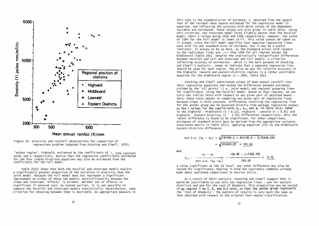
Figure 10. Erosivity and rainfall observations for comparison ofregressions problem (adapted from Stocking and Elwell, 1976).

'anchor region', highveld, estimated by the coefficients of X9 (the constantterm) and X respectively. Notice that the regression coefficients estimatedfor the four simple bivariate equations may also be estimated from thecoefficients for the Full model.

Table 10(b) shows that both the Parallel and Intercept models explaina significantly greater proportion of the variation in erosivity than theJoint model. Because the Full model does not represent a significantimprovement on either of these two models, multicollinearity between theslope and intercept 'effects' is evident. Neither set of effects issignificant if entered last. As stated earlier, it is not possible tocompare the Parallel and Intercept models statistically. Nevertheless, somecriterion for choosing between them is desirable. An appropriate measure in

36

this case is the standard error of estimate, s, obtained from the squareroot of the residual mean square estimated for the regression model inquestion, and reflecting the accuracy with which values of the dependentvariable are estimated. These values are also given in Table 10(a). Usingthis criterion, the Intercept model fares slightly better than the Parallelmodel, their s values being 1610 and 1596 respectively. However, the valueof 1584 for the Full model is lower still. This value cannot be taken asit stands, since the Full model specifies four separate regression lines,each with its own standard error of estimate, but it may be a usefulindicator. It proves to be so here, as the standard errors with respectto the individual lines are less than 1584 for all regions except themiddleveld (Table 10a). Despite the statistically insignificant differencesbetween Parallel and Full and Intercept and Full models, a criterionreflecting accuracy of estimation - which is the main purpose of Stockingand Elwell's analysis - seems to indicate that a separate regression lineshould be used for each region. The price we pay for relative accuracy inthe highveld, lowveld and eastern districts regions is a rather unreliableequation for the middleveld region (s = 1865, Table 10a).

Stocking and Elwell substituted values of mean annual rainfall intotheir regression equations and tested the differences between estimatesyielded by the 'all points' (i.e. Joint model) and regional grouping linesfor significance. Using the Parallel model, based on four regions, we cancarry out similar tests with respect to any given pair of adjusted means -here, these tests amount to comparing any given pair of regression linesbecause slope is held constant. Differences involving the regression linefor the anchor group may be assessed directly from package regression output,

to the Highveld - Middleveld (t = 0.12), Highveld - Lowveld (t = 0.45) andHighveld - Eastern Districts (t 3.54) differences respectively. Only thelatter difference is found to be significant. For other comparisons,estimates of standard errors must be derived from the appropriate variance-covariance matrix in Table 10(c). Applying equation (23) to the Middleveld-Eastern Districts difference:

a value significant at the 1% level. Any other difference may also betested for significance, bearing in mind the cautionary comments alreadymade about unplanned comparisons in Section IV(iv).

As a result of their analysis, Stocking and Elwell suggest that itwould be justifiable to use only two regression lines - one for easterndistricts and one for the rest of Rhodesia. This proposition may be tested

the 'rest of Rhodesia'. The pattern of results is very much the same asthat obtained with respect to the original four-region classification,

37

multicollinearity between slope and intercept effects again being present(Table lla,b).

Table 11. Results for two regions

(a) Estimation of parameters

Comparing the Full model based on four regions with the Parallel,Interceptand Full models based on two regions - eastern and the rest of Rhodesia -no significant differences can be found, thus supporting the proposition(Table 11c). Comparison of standard errors produces yet another unequivocalresult, since the value for the 'rest of Rhodesia' is relatively high(s = 1672) and exceeded only by that for the individually derived equationfor the middleveld (s 1865, Table 10a).

38

Figure 11. Mean annual erosivity over Rhodesia estimated from regressionequations (redrawn from Stocking and Elwell, 1976).

Stocking and Elwell applied the four separate regression equations ofTable 10(a) to the mean annual rainfall map of Rhodesia, converting theisohyets to isopleths of erosivity. The resulting 'erosivity map' isreproduced in Figure 11. Remember that the extreme high and low erosivityvalues have been exaggerated by Stocking and Elwell because of their regress-ion of X on Y rather than Y on X.

If one of the Parallel or Intercept models for the four-region case hadproved superior in terms of accuracy of estimation, how would the erosivityestimates have been obtained? Taking the Parallel model as an example, theestimating equation for the anchor region highveld, according to Table 10(a),is:

Corresponding to a mean annual rainfall of, say, 600mm, we obtain erosivity

estimates of

39

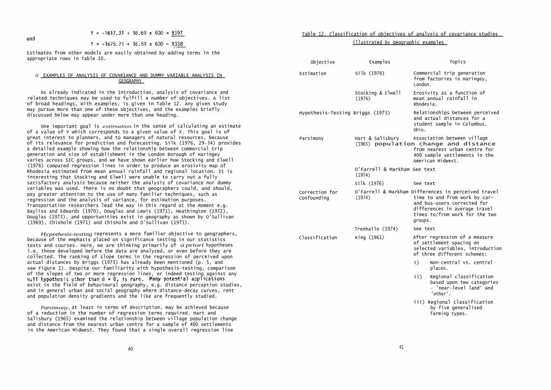
Estimates from other models are easily obtained by adding terms in theappropriate rows in Table 10.

VI EXAMPLES OF ANALYSIS OF COVARIANCE AND DUMMY VARIABLE ANALYSIS IN GEOGRAPHY

As already indicated in the Introduction, analysis of covariance andrelated techniques may be used to fulfill a number of objectives. A listof broad headings, with examples, is given in Table 12. Any given studymay pursue more than one of these objectives, and the examples brieflydiscussed below may appear under more than one heading.

One important goal is estimation in the sense of calculating an estimateof a value of Y which corresponds to a given value of X. This goal is ofgreat interest to planners, and to managers of natural resources, becauseof its relevance for prediction and forecasting. Silk (1976, 29-34) providesa detailed example showing how the relationship between commercial tripgeneration and size of establishment in the London Borough of Haringeyvaries across SIC groups, and we have shown earlier how Stocking and Elwell(1976) compared regression lines in order to produce an erosivity map ofRhodesia estimated from mean annual rainfall and regional location. It isinteresting that Stocking and Elwell were unable to carry out a fullysatisfactory analysis because neither the analysis of covariance nor dummyvariables was used. There is no doubt that geographers could, and should,pay greater attention to the use of many familiar techniques, such asregression and the analysis of variance, for estimation purposes.Transportation researchers lead the way in this regard at the moment e.g.Bayliss and Edwards (1970), Douglas and Lewis (1971), Heathington (1972),Douglas (1973), and opportunities exist in geography as shown by O'Sullivan(1969), Chisholm (1971) and Chisholm and O'Sullivan (1973).

Hypothesis-testing represents a more familiar objective to geographers,because of the emphasis placed on significance testing in our statisticstexts and courses. Here, we are thinking primarily of a priori hypothesesi.e. those developed before the data are analyzed, or even before they arecollected. The ranking of slope terms in the regression of perceived uponactual distances by Briggs (1973) has already been mentioned (p. 5, andsee Figure 1). Despite our familiarity with hypothesis-testing, comparisonof the slopes of two or more regression lines, or indeed testing against any

exist in the field of behavioural geography, e.g. distance perception studies,and in general urban and social geography where distance-decay curves, rentand population density gradients and the like are frequently studied.

Parsimony, at least in terms of description, may be achieved becauseof a reduction in the number of regression terms required. Hart andSalisbury (1965) examined the relationship between village population changeand distance from the nearest urban centre for a sample of 400 settlementsin the American Midwest. They found that a single overall regression line

40

Table 12. Classification of objectives of analysis of covariance studies

illustrated by geographic examples

Objective Examples Topics

Estimation Silk (1976) Commercial trip generationfrom factories in Haringey,London.

Stocking & Elwell Erosivity as a function of(1976) mean annual rainfall in

Rhodesia.

Hypothesis-Testing Briggs (1973) Relationships between perceivedand actual distances for astudent sample in Columbus,Ohio.

Parsimony Hart & Salisbury Association between village(1965) population change and distance

from nearest urban centre for400 sample settlements in theAmerican Midwest.

O'Farrell & Markham See text(1974)

Silk (1976) See text

Correction for O'Farrell & Markham Differences in perceived travelConfounding (1974) time to and from work by car-

and bus-users corrected fordifferences in average traveltimes to/from work for the twogroups.

Trenhaile (1974) See text

Classification King (1961) After regression of a measureof settlement spacing onselected variables, introductionof three different schemes:

i) Non-central vs. centralplaces.

ii) Regional classificationbased upon two categories- 'near-level land' and'other'.

iii) Regional classificationby five generalisedfarming types.

41

(Joint Model) could be substituted for the nine regression lines - one foreach individual state. Similarily, O'Farrell and Markham (1974) were ableto substitute one regression equation for the two initially obtained in astudy of the relationship between actual and perceived waiting times withrespect to car and bus-users in Dublin. Silk (1976, 29-33) showed how nineseparate regression lines could be reduced to a 'hybrid' model consistingof three regression lines with different slopes but a common intercept,plus a free-standing regression line representing one 'deviant' category.

Correction for confounding is a rarely mentioned objective in thegeographic literature, although examples may be found in O'Farrell andMarkham (1974) and Silk (1976, 19-23). Trenhaile (1974) concluded that anydifference between shore platform gradients developed on chalk bedrockcompared with those developed in lias sandstones and shales was statisticallyinsignificant if allowance were made for variations in tidal range.Relationships between platform gradient and other variables, such as fetch,were analyzed in the same way.

Last, but not least, the technique may be used as an aid to classifica-tion. No matter whether a set of categories has been derived a priori orrepresents the fruit of opportunism as research proceeds, it is possibleto construct and test statistically classification schemes based on regress-ion models. Most of the papers in Section B of the references providegood examples of this particular use of covariance analysis, and may alsobe regarded as exploratory in the sense that identification of, andstatistical testing for, empirical regularities are based on the same dataset (Hauser, 1974). Particularly clear discussions of this process ofexploration may be found in King (1961), Kariel (1963) and Yeates (1965).

Two comments on procedure may be made here. First, almost all studiesconcentrate upon comparison of Joint, Parallel and Full models. Admittedly,there are more situations in which we should be pleased to discover thata number of separate regression lines have a common slope, but considerablesimplification is also possible if a common intercept can be identified.Second, geographers invariably approach analysis of covariance by way ofregression analysis. Essentially, an analysis of variance is carried outon the residuals about a single regression plane. Although the analysisis carried out 'backwards' in terms of the scheme of comparisons outlinedpreviously, there is no reason why the whole process should not be carriedout taking the Joint model as its starting point.

A list of studies which employ dummy variable analysis is given inSection C of the references.

VII COMPUTER ROUTINES

A number of standard computer package programmes is available forcarrying out the analysis of variance and covariance. The StatisticalPackage for the Social Sciences (SPSS) provides a useful discussion of thesetechniques as well as the programs in Chapter 22 of the manual (Nie et al,1975); the library of Biomedical (BMD) Computer Programs is another widelyavailable alternative (Dixon, 1968, 285-304; 597-605; 705-718). To implementthe BMD programs on one of the ICL 1900 series of computers, it is

42

necessary to refer to the appropriate Numerical Algorithms Group (NAG)NIMBUS manual. NAG routines for the analysis of variance are also available.

Routines which automatically provide the output required to compareregression lines do not appear to be generally available. The author usedtwo ALGOL programmes, ASA6 and ASA9, written by members of the Departmentof Applied Statistics at the University of Reading, to check resultsobtained using dummy variables and multiple regression routines. Summaryinformation on residual sums of squares and degrees of freedom for 'between'comparisons in the bivariate case is given by ASA6, and in the multivariatecase by ASA9. The SPSS manual does, however, provide a full discussion ofdummy variable analysis, with examples (Nie et al; 1975, Chapter 21).

Standard multiple regression routines may be used to carry out all thecomparisons 'between' and 'within' models described earlier. If suchroutines are employed a print-out of the variance-covariance matrix isusually available, thus enabling 'within' comparisons to be made betweenany given pair of intercepts or slopes. The writer exclusively usedmultiple regression routines, because of the great flexibility possible ifdummy variables are employed, e.g. combining of existing categories orcreation of new categories.

References to computer program descriptions are given in Section A.

VIII FURTHER EXTENSIONS AND CONCLUSION

The scope of the technique may be extended in various ways. First,by adding one or more categorical independent variables; second, by addingone or more continuous independent variables - this was the strategy adoptedby Yeates (1965) to compare multiple regression equations between six radialsectors in Chicago; third, by adding both categorical and continuousvariables.

All three extensions, but particularly the first and the last, mayrequire a large number of observations, first, because two-(or higher)way analysis of variance, or its dummy variable equivalent, are expensivein terms of degrees of freedom and, second, to ensure that there are noempty cells in the cross-classification. It is worth noting that theeffects in an n-way analysis of variance may be estimated using dummyvariable technique if we need to deal with a cross-classification schemewith unequal numbers of observations in the cells, a situation which theconventional estimation procedure cannot handle. Further discussion of theseissues may be found in Goldberger (1964, 227-231), and worked examples inSnedecor and Cochran (1967, ch. 14).

There are many branches of geography within which the analysis ofcovariance, and the associated techniques for comparison of regression lines,may be profitably employed. Technically, there are few obstacles to theirmore widespread use since the underlying statistical theory is well-developed,and a number of different computing procedures is available.

43

BIBLIOGRAPHY

A. Technical papers and computer programs

Blalock, H.M. (Jr) (1964), Causal inferences in nonexperimental research.(Chapel Hill: University of North Carolina Press).

Blalock, H.M. (Jr) (1972), Social statistics (International student edition).(New York: McGraw-Hill), ch. 20.

Cohen, J. (1968), Multiple regression as a general data-analytic system.Psychological Bulletin, 70, 426-443.

Davidson, N. (1976), Causal inferences from dichotomous variables.Concepts and techniques in modern geography,9. (Norwich:Geo Abstracts Ltd.).

Davies, 0.L. (ed) (1961), Statistical methods in research and production.(Edinburgh: Oliver and Boyd).

Dixon, W.J. (ed) (1968), Biomedical computer programs. (California:University of California Press).

Draper, N.R., and Smith, H. (1966), Applied regression analysis.(New York: Wiley).

Ferguson, R. (1978), Linear regression in geography, Concepts and techniquesin modern geography, 15. (Norwich: Geo Abstracts Ltd.).

Goldberger, A.S. (1964), Econometric theory. (New York: Wiley).

Goldberger, A.S. (1968), Topics in regression analysis. (New York: MacMillan),ch. 8.

Hauser, D.P. (1974), Some problems in the use of stepwise regressiontechniques in geographical research. Canadian Geographer,18, 148-158.

Jennings, E. (1967), Fixed effects analysis of variance by regressionanalysis. Multivariate Behavioural Research, 2, 95-108.

Johnston, J. (1963), Econometric methods (International student edition).(New York: McGraw-Hill), ch. 8.

Kerlinger, F., and Pedhazur, E.J. (1973), Multiple regression in behavioralresearch. (New York: Holt, Rinehart and Winston), chs. 6-11.

Kirk, R.E. (1972), Statistical issues: a reader for the behavioral sciences.(Belmont, California: Brooks/Cole).

Nie, N., Bent, D.H., and Hull, C.H. (1975), Statistical package for thesocial sciences (SPSS). (New York: McGraw-Hill).

Selvin, H.C., and Stuart, A. (1966), Data dredging procedures in surveyanalysis. The American Statistician, June 20-23.

Silk, J.A. (1976), A comparison of regression lines using dummy variableanalysis. Geographical Paper, 44. (Reading: Department ofGeography, University of Reading).

Snedecor, G.W., and Cochran, W.G. (1967), statistical methods. (Ames, Iowa:Iowa State University Press).

Suits, D.B. (1957), The use of dummy variables in regression equations.Journal of the American Statistical Association, 52, 548-551.

44

Taylor, P.J. (1969), Causal models in geographic research. Annals of theAssociation of American Geographers, 59, 402-404.

Unwin, D.J. (1975), An introduction to trend surface analysis. Conceptsand techniques in modern geography, 5. (Norwich: GeoAbstracts Ltd.).

Weatherburn, C.E. (1962), A first course in mathematical statistics.(Cambridge University Press), (2nd edition).

Wrigley, N. (1976), An introduction to the use of logit models in geography.Concepts and techniques in modern geography, 10, (Norwich:Geo Abstracts Ltd.).

B. Applications of analysis of covariance

Briggs, R. (1973), Urban cognitive distance, 361-390 in: Downs, R.M., andStea, D. (eds), Image and environment. (London: Arnold).

Carey, L., and Mapes, R. (1972), The sociology of planning (London: Batsford),ch. 4.

Dogan, M. (1969), A covariance analysis of French electoral data. 285-298 inDogan, M., and Rokkan, S. (eds), Quantitative ecological analysisin the social sciences. (Cambridge Mass: MIT Press).

Doornkamp, J.C., and King, C.A.M. (1970), Numerical analysis in geomorphology,(London: Arnold).

Garner, B.J. (1966), The internal structure of retail nucleations.Northwestern University Studies in Geography, 12. (Evanston,Illinois: Department of Geography, Northwestern University).

Hart, J.H., and Salisbury, N.E. (1965), Population changes in MiddleWestern villages: a statistical approach. Annals of theAssociation of American Geographers, 55, 140-160.

Kariel, H.G. (1963), Selected factors areally associated with populationgrowth due to net migration. Annals of the Association ofAmerican Geographers, 53, 210-223.

King, L.J. (1961), A multivariate analysis of the spacing of urban settlementsin the United States. Annals of the Association of AmericanGeographers, 51, 222-233.

O'Farrell, P.N., and Markham, J. (1974), Commuter perceptions of publictransport work journeys. Environment and Planning, A6, 79-100.

Trenhaile, A.S. (1974), The geometry of shore platforms in England and Wales.Transactions, Institution of British Geographers, 62, 129-142.

C. Applications of dummy variables and comparisons of regression lines

Bayliss, B.T., and Edwards, S.L. (1970), Industrial demand for transportLondon: H.M.S.O.

Blaikie, P.M. (1973), The spatial structure of information networks andinnovative behaviour in the Ziz valley, Southern Morocco.Geographiska Annaler, 55B, 83-105.

Cheshire, P. (1973), Regional unemployment differences in Great Britain.in Cheshire, P. (ed) Regional papers II. National Institute forEconomic and Social Research, (Cambridge: Cambridge UniversityPress).

45

Chisholm, M. (1971), Freight transport costs, industrial location andregional development. 213-244 in Chisholm, M., and Manners, G.(eds), Spatial policy problems of the British economy.Cambridge:(Cambridge University Press).

Chisholm, M., and O'Sullivan, P. (1973), Freight flows and spatial aspectsof the British economy. (Cambridge: Cambridge University Press).

Douglas, A.A., and Lewis, R.J.(1971), Trip generation techniques:household least-squares regression analysis. Traffic Engineeringand Control, 12, 477-479.

Douglas, A.A. (1973), Home-based trip models - a comparison between categoryanalysis and regression analysis procedures. Transportation,2, 53-70.

Hannell, F.G. (1973), The thickness of the active layer on some of Canada'sarctic slopes. Geografiska Annaler, 55A, 177-184.

Heathington, K.W. and Isibor, E. (1972), The use of dummy variables in tripgeneration analysis. Transportation Research, 6, 131-142.

Knos, D.S. (1968), The distribution of land values in Topeka, Kansas.269-289 in Berry, B.J.L., and Marble, D.F. (eds), Spatialanalysis. (Englewood Cliffs: Prentice-Hall).

Lee, T.H. (1963), Demand for housing: a cross section analysis. Review ofEconomics and Statistics, 45, 190-196.

O'Sullivan, P. (1969), Transport networks and the Irish economy. (London:Weidenfield and Nicholson, London School of Economics).

Orcutt, G.H., Greenberger, M., Korbel, J., and Rivlin, A.M. (1961),Micro-analysis of socio-economic systems: a simulation study.(New York: Harper and Row).

Silk, J.A. (1976), A comparison of regression lines using dummy variableanalysis. Geographical Paper, 44, (Reading: Department ofGeography, University of Reading).

Starkie, D.N.M. (1970), The treatment of curvilinearities in the calibrationof trip-end models. In Urban Traffic Model Research.London: Planning, Transportation Research and Computation Ltd.(PATRAC).

Starkie, D.N.M., and Johnson, D.M. (1975). The economic value of peace andquiet. (Farnborough: Lexington Books/D.C. Heath).

Stocking, M.A., and Elwell, H.A. (1976), Rainfall erosivity over Rhodesia.Transactions, Institute of British Geographers (New Series),1(2), 231-245.

Vickerman, R.W. (1974). A demand model for leisure travel. Environment andPlanning, 6, 65-77.

Yeates, M.N. (1965), Some factors affecting the spatial distribution ofChicago land values, 1910-1960. Economic Geography, 41(1),57-70.

46