Advanced Topic in Astrophysics, Lecture 1

Radio Astronomy - Antennas

Phil Diamond, University of Manchester

Course Structure

•Modules– Module 1, lectures 1-6 (Phil Diamond, Maria Rioja)

• Mon March 1, 8, 15: 3 double lectures• Radio astronomy: antennas, interferometry and VLBI

– Module 2, lectures 7-12 (J-P Macquart)• Radiation Mechanisms I: 3 double lectures, dates TBD

– Module 3, lectures 13-18 (J-P Macquart)• Radiation Mechanisms II: 3 double lectures, dates TBD

– Module 4, lectures 19-24 (Ken Freeman)• Dynamics of the Milky Way• Dates TBD

Resources

•ATNF Synthesis Imaging workshops 2003, 2006– http://www.atnf.csiro.au/whats_on/workshops/synthesis2006/prog.h

tml

•Texts–Radio Astronomy: Kraus–Tools of Radio Astronomy: Rohlfs & Wilson–Interferometry and Synthesis in Radio Astronomy,

Thompson, Moran & Swenson.–Very Long Baseline Interferometry and the VLBA: Napier,

Diamond & Zensus., ASP Conf series, Vol 82, 1995.

Outline

•Imaging–Resolution–Direct and indirect imaging

•Telescopes–Parabolic and hyperbolic

•The Antenna–Horns and receivers

•Radio astronomy fundamentals and tools of the trade–Brightness temperature–Flux density–Radiometer equation

Direct imaging onto a focal plane

2” 10’1’

Resolution Δθ

2’’

Diffraction limits

Δθ=1” λ D

Optical 500 nm 125 mm

Radio 20 cm 50 km

Δθ=1.22 λ/D

Direct and indirect imaging

•Direct imaging–Normal imaging method whereby an image is projected onto

a detector.–Examples: camera, telescope, single-dish radio telescope

•Indirect imaging–Used where we cannot form a direct map of the object on the

focal plane.–We infer the properties of the object from certain

characteristics of the received electromagnetic field.–Examples: interferometry, NMR, ultrasound, PET, speckle.

A parabolic reflector adds all the fields from a surface(aperture) at a single focal point.

Parabolic reflector:

Direct Imaging: Single dish radio telescope

Direct Imaging - Angular Resolution•Angular Resolution (radians)

•Wavelength, λ=0.21m, D=64m

–⇒θ=0.003 rad, or 11 arcmin•Such a radio telescope only matches the resolution of the human eye at its shortest wavelength 1-2cm.

θ = λD

D

A radio telescope at Parkes, NSW (prime focus)

Hyperbolic reflector

.

B

.A

Light from the point A reflecting off the hyperbola appears to come from point B

Parabolic reflector

Prime Focus

Hyperbolic reflector

Parabolic reflector

Classical Cassegrain

AT antenna:

•Cassegrain configuration

•22-m diameter primary main reflector

•2.75-m secondary reflector

Offset Cassegrain

Beam Waveguide

Prime Focus

Naysmith

Cassegrain Focus

Dual offset

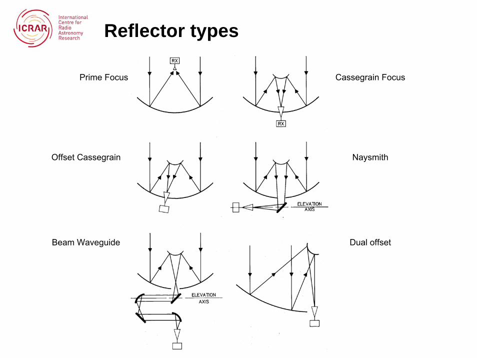
Reflector types

Offset Cassegraine.g. VLA and

ALMA

Beam Waveguidee.g. NRO

Prime Focuse.g. GMRT

Naysmithe.g. OVRO

Cassegrain Focuse.g. Mopra (AT),

e-MERLIN

Dual offsete.g. ATA

Reflector types

Signal path:

Signal path:

The antenna collects the E-field over the aperture at the focus

The focus is a fixed spot at all frequencies.

The reflector antenna is achromatic.

EM-wave electric field oscillations induce voltage oscillations at the antenna focus, in a device called a feed.

Feeds are ‘compact’ and ‘corrugated’ hornsThe inner profile is curved The inner surface has grooves in

order to increase the surface impedance, so that the wave does not set up voltages in the surface material, but is channelled into a dipole at the end of the horn.

Cross-section of a horn

Brightness Temperature

Radio photons are pretty wimpy:

Radio photons are too wimpy to do very much - we cannot detect individual photons

e.g. optical photons of 600 nanometre => 2 eV or 20000 Kelvin (hv/kT)

e.g. radio photons of 1 metre => 0.000001 eV or 0.012 Kelvin

Photon counting in the radio is not an option, must think classically in terms of electric fields, i.e. the best we can do is for the incoming EM-wave electric field oscillations to induce voltage oscillations in a conductor.

Brightness Temperature

•In radio astronomy T is known as the brightness temperature.

•Radiation mechanisms in radio astronomy are often non-thermal, but this does not stop astronomers talking about the “brightness temperature” of a source: i.e. the equivalent or effective temperature that a blackbody would need to have in order to be that bright!

Solid angle of source, Ω

1 Jansky (Jy) = 10-26 W m-2 Hz-1

Radio photons are pretty wimpy:

Rayleigh-Jeans Law:Iν α ν2

Examples of brightness temperatures:

“Blank” sky ~ 2.73 K (big bang BB radiation)

Sun at 300 MHz, 500000 K

Orion Nebula at 300 GHz ~ 10-100 K (“warm”molecular clouds)

Quasars at 5 GHz ~ 1012 K (synchrotron)

Brightness Temperature

Brightness temperature

• However, the giant pulses observed from the Crab Pulsar have Tb ~ 1034K

Orion H2O super-maser: Tb > 1018 K

The antenna aperture efficiency = Power collected by feedPower incident on antenna

There are many different potential loss factors:

Surface efficiency

~ 0.8

Aperture blockage efficiency

~ 0.8

Feed spillover efficiency

~ 0.8

Feed illumination efficiency ~

0.8

Misc. - other minor losses e.g feed mis-

match.

Feed

Spillover past main reflector (ray C)

Spillover past the sub-reflector (ray A)

Blockage of antenna surface by sub-reflector

~ 0.4 <==

Feed does not illuminate all of antenna surface equally

Antenna Performance

Antenna Temperature and Gain

• Antenna temperature is same as brightness temperature only if the source fills the antenna beam, e.g.

Ta ~ Tb x beam filling factor

•Examples

– Parkes 64-m antenna (η=60%): G=0.7 K Jy-1

– SKA 1km2: G=362 K Jy-1

Solid angle of antenna patternΩA

Antenna surface efficiency

According to the Ruze (1966) formula, the surface efficiency of a paraboloid is well described by:

where sigma is the r.m.s. error in the surface of the antenna.

e.g. For a surface efficiency of 0.7 (typical target value), therequired surface error (r.m.s.) is ~ lambda/20.

Or re-arranging:

==> at 7 mm (43 GHz) the surface accuracy must be ~ 350 micron.

==> many different forces acting on an antenna and its surface...

How can we possibly achieve a 350 µm accuracy (the thickness of three human hairs) – over a 100 metre diameter surface – an area equal to 2 football fields!

==> “active surface”.

Appreciating the scale of large radio telescopes....

GBT Surface has 2004 panelsaverage panel rms: 68µm.2209 precision actuators are located under each set of surface panel corners

Actuator Control Room (left): 26000 control and supply wires terminate in this room!

How big can parabolic telescopes be?

As the size (diameter) of a radio telescope increases, the gravitational and wind loads on the structure become difficult to manage. The worst problem is the problem of surviving a gale-force wind. The degree of wind distortion between paraboloids of different diameters (D) scales as D3.

The cost of antennas also scales roughly as D3.

Telescopes like the Jodrell Bank Mark V (right) with a diameter of ~ 305 metres (1970), will probably always remain in model form!

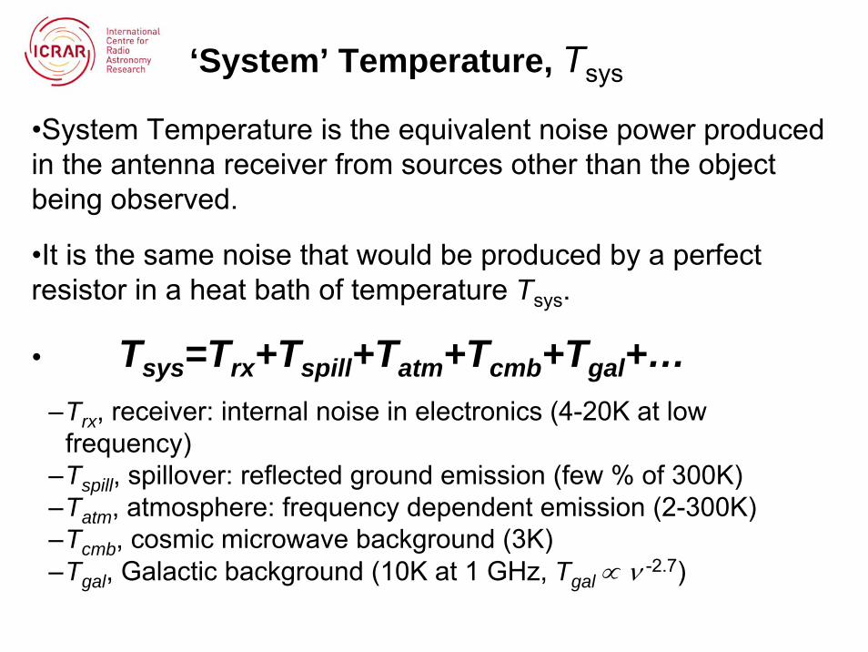
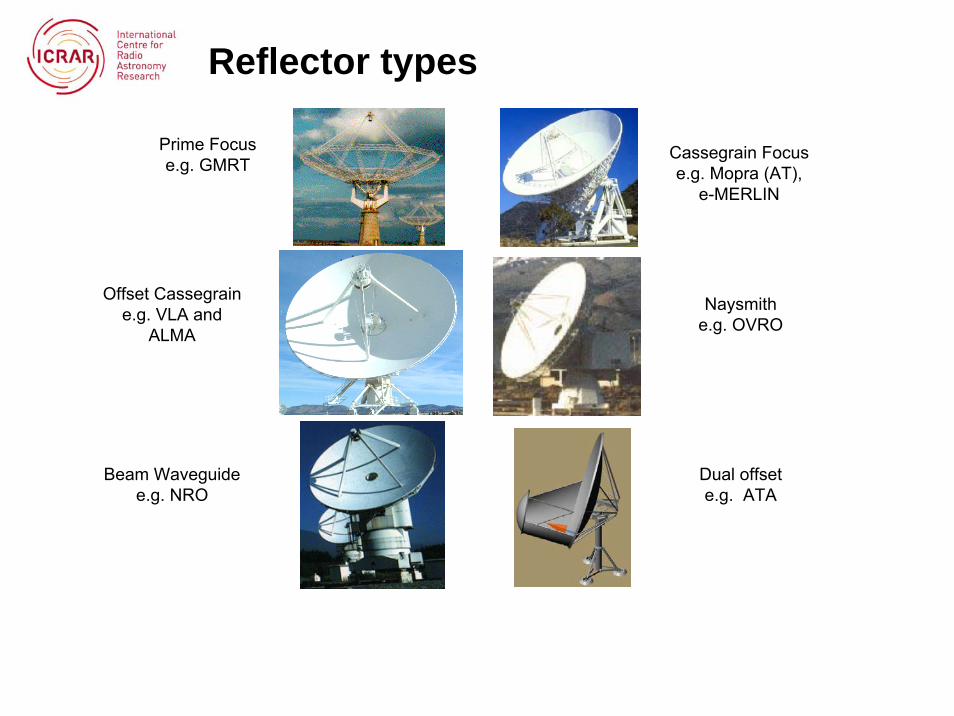
‘System’ Temperature, Tsys

•System Temperature is the equivalent noise power produced in the antenna receiver from sources other than the object being observed.

•It is the same noise that would be produced by a perfect resistor in a heat bath of temperature Tsys.

• Tsys=Trx+Tspill+Tatm+Tcmb+Tgal+…–Trx, receiver: internal noise in electronics (4-20K at low

frequency)–Tspill, spillover: reflected ground emission (few % of 300K)–Tatm, atmosphere: frequency dependent emission (2-300K)–Tcmb, cosmic microwave background (3K)–Tgal, Galactic background (10K at 1 GHz, Tgal ∝ ν -2.7)

p.32

Temperature sensitivity

•Radiometer equation

ΔT = Temperature sensitivity (K); T = System temperature (K);

τ= Integration time (s); Δν = Bandwidth (Hz)

•T=20K, τ=7200 sec, Δν=200 MHz ⇒ ΔT=50μK !

•System temperature describes the signal a telescope ‘sees’ if looking at a blackbody of temperature T which fills the field of view. NOT physical temperature.

ΔT =TτΔν

Other parts of telescope system

Radio Telescope Block Diagram

Radio Source

Receiver

FrequencyConversion

Signal Processing

SignalDetection

ComputerPost-detection

Processing

Antenna

Heterodyne system with LNAs,mixers etc

Bolometers, e.g. SCUBA-2

Other Antenna types

Dipoles Yagi

Helix

Log-periodic

The Jodrell Bank Mark 2 telescope (1964). Was considered to be a prototype of the then planned giant 300-metre MkIV. The aperture is elliptical -the idea was that a 300-metre would require an elliptical surface in order to reduce the height of the structure off the ground.

Some less conventional (weird!)reflector types

The off-axis cylinder radio telescope at Ooty. India (1970)

The big-ear antenna built by Kraus:

Other similar examples: Ratan 600 - Russia

Nancay (France):

Instead of building an entire parabola, Cross Antennas employ only a narrow section of a parabola, we get a beam narrow in the antenna’s wide direction, and broad in the other direction: .

Cross antennas

By observing a source with two orthogonal beams, we can get a 2-d image of the sky.

The cross antenna response is similar to the crossing point of the two beams (but with very high side-lobes):

The first Cross telescope - was built by Bernie Mills in Australia.

The Mills cross:

Molonglo cross

Northern cross (Bologna)

The 305-m Arecibo telescope is fixed in the ground. A spherical reflector is therefore employed:

Northern cross (Bologna)

While a parabola has a single focus point, a spherical reflector focus the incoming radio waves on a line:

Northern cross (Bologna)

By having a moving secondary a spherical reflector can be pointed in different (but still somewhat limited) directions on the sky.

Note that only part of the total surface area is useable for any given direction.

Part of the primary:

Northern cross (Bologna)

Looking on to the surface: quite a lot of litter!

Northern cross (Bologna)

While a parabola has a single focus point, a spherical reflector focus the incoming radio waves on a line:

Northern cross (Bologna)

By having a moving secondary a spherical reflector can be pointed in different (but still somewhat limited) directions on the sky.

Note that only part of the total surface area is useable for any given direction.

Arecibo is built in a karst depression. The Gregorian secondary hangs on cables that are supported by 3 large towers:

Northern cross (Bologna)

Horn antennas:

The reflecting “ear” reflects the incoming radio waves towards a horn or bare dipole.

Horn antennas have many practical applications - they are used in short-range radar systems, e.g. the hand-held radar “guns” used by policemen to measure the speeds of approaching or retreating vehicles.

The Horn Antenna combines several ideal characteristics: it is extremely broad-band, has calculable aperture efficiency, and the sidelobes are so minimal that scarcely any thermal energy is picked up from the ground. Consequently it is an ideal radio telescope for accurate measurements of low levels of weak background radiation.

A very famous example is the horn antenna located at Bell Telephone Laboratories in Holmdel, New Jersey, used by Penzias and Wilson to detect the relic radiation of the big bang.

The Bell Telephone Laboratories horn in Holmdel, New Jersey. Note the rotation axis that permits the horn to be directed at different points in the sky.

Things I have not touched upon

• Array receivers, focal plane phased arrays, aperture arrays

• Antenna pointing, servo control, holography, receiver stability, radomes, dielectric lenses, frequency conversion, time and frequency standards, ADCs, signal processing, data transmission

• Post-processing: pulsar searches, pulsar timing, spectroscopy, continuum, single-dish imaging

• RFI, spectrum management, radio quiet zones

• + …..

ASKAP

chequer board array

Things I have not touched upon

• Array receivers, focal plane phased arrays, aperture arrays

• Antenna pointing, servo control, holography, receiver stability, radomes, dielectric lenses, frequency conversion, time and frequency standards, ADCs, signal processing, data transmission

• Post-processing: pulsar searches, pulsar timing, spectroscopy, continuum, single-dish imaging

• RFI, spectrum management, radio quiet zones

• + …..

ASKAP

chequer board array