Patrizia

AEROACOUSTICS

A numerical approach to aerodynamic noise of aircraft wingsJ.W. Delfs

Institut für Aerodynamik und Strömungstechnik, Technische AkustikDLR - Deutsches Zentrum für Luft- und Raumfahrt e.V.

Lilienthalplatz 7, D-38108 Braunschweig, Germany

In view of the need for quiet aircraft design, computational tools have to be developed, capable of describing the noise generation pro-cess for airframe noise correctly. A respective simulation concept based on Computational Aeroacoustics (CAA) and linearized EulerEquations is presented and discussed. In the context of airframe noise the question of linearity of sources is addressed. Employing theproposed ”vortex test” simulation concept an aeroacoustic assessment of the thickness effect of airfoils in unsteady inflow conditionsis presented.

INTRODUCTION

The sound generated in unbounded unsteady subsonicflow is marginal in intensity compared to the excess noiseproduced when such unsteady flow interacts with finiteaerodynamic bodies. In airframe noise problems, suchunsteadiness is usually associated with turbulence. Abody may be understood as a disturbance to the dynam-ics of the unsteady flow components, associated with acorresponding change in the pressure field. This changeis usually large near inhomogeneities of the boundary(edges, slots, humps, steps etc.) and it is accompaniedby the conversion of part of the hydrodynamic -usuallyturbulent- pressure fluctuation into sound pressure. More-over, sources of this kind represent particularly efficientsound emitters for frequencies with respect to which thegeometric body components appear non-compact. Allthese conditions are usually satisfied for the deployedhigh lift devices on the wing of a typical modern civilaircraft in approach. As verified in numerous flight- andwindtunnel tests the most intense sources of airframenoise are indeed found near the leading-, trailing- andside edges of the slat and flap when located by meansof microphone arrays [3] or elliptic mirrors [2].

The computation of airframe noise may be approachedin different ways. The most classical one is to solve an in-homogeneous acoustic wave equation for a given sourceterm (e.g. Lighthill’s tensor as volume source, surfacepressure fluctuations as a surface source etc.). The issuehere is, that by definition all vortex dynamics (the orig-inator to sound generation) lies buried inside the sourceterm and thus has to be known in advance. Typically, forsimple cases the source term is modelled or -if availabe-extracted from DNS data. It is noted, that any domain,where the wave equation is not satisfied (e.g. inside arefracting shear layer) is to be understood as a source re-gion, requiring some source term.

The second way to compute airframe noise involvesthe direct numerical solution of the balance equations for

mass, momentum and energy and is usually refered toas CAA-simulation. The characteristic difference to thewave equation approach is, that apart from the acousticdegrees of freedom, the vortical (and entropic) degreesof freedom of the fluid dynamics is allowed for. In thisway the conversion process from vorticity to sound andvice versa is incorporated into to theoretical description.Although the CAA-approach is usually associated withquite an increase in computation cost, it has importantadvantages, namely a) that the sound generation is sim-ulated, rather than modelled and b) that sound propaga-tion through arbitrary flow fields is described properly. Inwhat follows a CAA-scheme is used to simulate unsteadyperturbations about a given steady mean flow field, alongwith the sound generation near aerodynamic bodies in-side this mean flow.

GOVERNING EQUATIONS

For a given (quasi-) steady flow field qqq0 : � �ρ0 � vvv0 � p0 � ,

with ρ-density, vvv-velocity vector, p-pressure, the invisciddynamics of small perturbations qqq � : � �

ρ � � vvv � � p � � aboutthis basic flow are governed by the linearised Euler equa-tions for a thermally and calorically perfect gas:

d0ρ �dt � vvv ��� � � ∇∇∇ρ0 � ρ0∇∇∇� � � vvv � � ρ � ∇∇∇ � � � vvv0 � m � (1)

ρ0 d0vvv �dt � ρ0vvv � � � � ∇∇∇vvv0 � ρ � vvv0 � � � ∇∇∇vvv0 � ∇∇∇p � � fff � (2)

d0 p �dt � vvv � � � � ∇∇∇p0 � γ p0∇∇∇� � � vvv � � γ p � ∇∇∇ � � � vvv0 � ϑ � (3)

Here, d0

dt : � ∂∂t � vvv0 � � � ∇∇∇ denotes the time derivative taken

along a streamline of the mean velocity field vvv0 and γis the isentropoc exponent (γ � 1 � 4 for air under normalconditions). The equations are dimensionless with thefollowing notation: time t � t a∞ l, lengths xi

� x i l,density ρ � ρ ρ∞, velocity vector vvv � vvv a∞, pressurep � p ρ∞a2

∞, a mass source density m � � m � l ρ∞a∞, a

body force density fff � � fff � � l � ρ∞a2∞ and an energy (e.g.

heat) source density ϑ � � ϑ � � l � ρ∞a3∞, where a � γp � ρ is

the speed of sound. The asterisk denotes quantities withdimensions and the quantities with an index ∞ mean ref-erences, which typically are freestream values of the flowquantities.

The boundary condition for acoustically hard walls isequivalent with satisfying the kinematic flow condition

vn : � nnn � � � vvv ��� 0 � (4)

where nnn is the normal vector on the considered wall point.The wall condition is not directly implemented into thedifference scheme but indirectly via the pressure gradi-ent following[4]. Taking the dot product of the momen-tum equation (2) with nnn and respecting (4) at a wall pointyields:

∂p �∂n

��� ρ0 � vvv0vvv ��� vvv � vvv0 � � ρ � vvv0vvv0 � ::: ∇∇∇nnn (5)

The normal derivative on the pressure is the product ofthe momentum fluxes with the local curvature tensor ofthe wall. The derivative vanishes when the wall is planeor there is no flow present.

NUMERICAL SOLUTION SCHEME

The differential equation system (1-3) is solved nu-merically subject to the given boundary and initial condi-tions. The temporal discretization is done with the clas-sical fourth order Runge-Kutta scheme (RK4). Spatialgradients are approximated using the dispersion relationpreserving 7-point stencil finite difference scheme (DRP)of Tam& Shen [5] and Tam& Dong[4], on curvilinear(block-) structured grids, see e.g. [6]. The physical gridis given as node sequence in the indices i � j

xxxi j � xxx � ξ � i � η � j � (6)

where ξ and η represent a uniform cartesian system andassume integer values on the nodes. For fixed ξ � I thegrid variable η defines a grid line and vice versa. Sincethe coefficients of the DRP scheme are defined for theuniform computation grid ξ � i, η � j the perturbationequations (1-3) need to be transformed from the physicaldomain to the computation domain ξ � η. This is done byreplacing ∇∇∇ by

∇∇∇ � MMM∇∇∇ξ (7)

where MMM � ∇∇∇ξξξ is the metric of the transform. It isobtained by inverting MMM � 1 � ∇∇∇ξxxx � ξ � η � , which is avail-able with high accuracy employing the DRP differencingscheme along the grid lines. The metric is needed accu-rately in order that the high resolution and accuracy prop-erties of the DRP scheme would be transferred into the

physical space. Overlapped grid systems are well suitedfor CAA [1] to facilitate gridding near complex geome-try components, since these are the source locations ofairframe noise.

Very short wave length components of the signalswhich cannot be represented physically correctly on thegiven computation grid are suppressed with artificial se-lective damping (ASD) due to Tam&Dong [7]. For eachof the equations of the system (1-3) the same symmet-ric linear, scalar damping operator D is introduced. Thesource terms on the right hand side of (1-3) are identi-fied with these damping terms acting as sinks rather thansources:

m ��� � νD � ρ � �fff ��� � νD � vvv � � (8)

ϑ ��� � νD � p � �with

D �"!#!#! �$��%%%%∂xxx∂ξ

%%%%� 2

Dξ �&!'!#! � � %%%%∂xxx∂η

%%%%� 2

Dη �"!#!#! �(! (9)

The coefficients of the 7-point stencil numerical opera-tor D are given in [7]; the subscripts on D indicate thegrid line direction along which the operator is to be ap-plied. The damping coefficient ν must be chosen suchthat i) non-physical, i.e. purely numerically caused sig-nal components are efficiently damped while affecting thephysical wave components as little as possible, and ii) nonumerical instability of the overall scheme is generated.

SIMULATION CONCEPT

Because of the wide range of turbulence scales, thenumerical prediction of airframe noise for technicallyrelevant flow Reynolds numbers is out of reach even ontoday’s largest high performance computers. In order toreduce the computational effort, it has become popularto pre-compute (by CFD) the steady viscous meanflow field qqq0 and to simulate by CAA only the inviscidperturbations qqq � . As in the wave equation approachthis again requires some modeling. The modeling ishowever reduced to an appropriate excitation of vorticityperturbations, rather than the whole aeroacoustic source.Here, an approach is presented in which upstream ofthe airframe component localized vorticity is introducedinto the flow field. In the course of the simulation themean flow convects the perturbation past the airframecomponent upon which sound is generated. The acousticresponse is measured far from the body. This simulationis repeated for varied geometry but the same initial testvorticity. Comparison of the acoustic responses thenallows for a noise assessment of airframe componentsin the following sense. The less efficient it converts

p’

FIGURE 1. Linear pressure field evolving from localized vor-tex, seeded at t ) 0 and x ) 2. Above: no wedge, below: withwedge at x ) 10. Wedge causing generation of sound.

vorticity into sound, the quieter the design. Note, that aproperty of a body (in fact a response function) is sought,rather than an absolute pressure level in dB.

Note on linearity

Before turning to examples a short note on the math-ematical character of airframe noise sources is in place,because the question arises, whether it is justified to uselinearized perturbation equations (1-3) for the descrip-tion airframe noise generation or whether airframe noisesources are fundamentally nonlinear. In order to addressthis issue reference is made to Lilley’s equation, whosewave operator is known to describe sound propagationthrough parallel shear flows. It reads

ddt

*d2Πdt2 + ∇∇∇ , , ,.- a2∇∇∇Π /1032 2t∇∇∇vvv:::∇∇∇ - a2∇∇∇Π /54

+ 2t∇∇∇vvv ::: - ∇∇∇vvv∇∇∇vvv /62 Ψ (10)

where Π 4 γ 7 1 ln - p 8 p∞ / is the acoustic variable, super-script t means ”transpose” and Ψ denotes terms of vis-cous friction and entropy, which are negligible for highReynolds numbers. The remaining aeroacoustic sourceterm due to Lilley is therefore Q 4 + 2t∇∇∇vvv ::: - ∇∇∇vvv∇∇∇vvv / .

Linearization of Lilley’s equation about a parallel meansteady flow field vvv0 4:9 u0 - y /.; 0 ; 0 < shows that the linearpart of Q vanishes identically, of which follows immedi-ately that sound generation in a parallel mean flow fieldis a fundamentally nonlinear problem.

This in turn means that the evolution of a linear vortexin a parallel shear layer is perfectly silent even whileinitiating a Kelvin-Helmholtz instability. This situationwas simulated using the linearized Euler equations (1-3)in a parallel shear layer with a realistic profile u0 - y /taken from a RANS-CFD simulation. The shearlayer islocated in + 1 = 1 > y > 1 = 1; below there is no flow andabove there is a constant flow of Mach number M 4 0 = 4.Localized vorticity is introduced at simulation time t 4 0and position x 4 2 ; y 4 + 0 = 5. As a result a downstreamconvecting unstable wave packet evolves representingthe classical Kelvin-Helmholtz instability. The upperpart of Fig. 1 shows the respective linear pressure fieldp ?@- x ; y ; t 4 70 / , which consists of purely hydrodynamic(i.e. non-propagating) components indicating completesilence and thus confirming the statement of Lilley’sequation. Next, the effect of the presence of a wedgeon the pressure field is considered. For this purpose asharp vertical wedge with vertex at x 4 10 ; y 4 + 1 = 4 isoriginally placed below the shearlayer and the simulationis repeated for otherwise identical parameters. In thiscase, shown in the lower part of Fig. 1, sound is generatedby scattering of the wave packet’s linear hydrodynamicpressure field at the wedge although the mean flow doesnot even touch the wedge. The example shows that in

x

y

-1 -0.5 0 0.5 1 1.5-0.5

0

0.5

x

y

-3 -2 -1 0 1 2 3 4

-3

-2

-1

0

1

2

3

p’ : -0.1 -0.05 -0.025 -0.01 0.01 0.025 0.05 0.1

v’ : -0.5 -0.4 -0.3 -0.2 -0.1 0.1 0.2 0.3 0.4 0.5

p’

v’

FIGURE 2. Vortex-airfoil interaction. above: v ACB t ) 3 D 5 E , be-low: p ACB t ) 3 D 5 E .

the presence of edges the sound generation by vorticitybecomes a linear problem and it is reasonable to studyairframe noise generation using linear equations (1-3).

APPLICATION TO GUST-AIRFOILINTERACTION

The presented simulation concept for a computationalassessment of airframe noise using CAA is applied forthe example of noise generated by an airfoil due to in-coming gusts. When a vorticity perturbation strikes theleading edge of an airfoil, sound is generated. A 2D-case is presented in Fig.2, showing the vertical veloc-ity v F and the pressure field p F well after a test vortexwas seeded into the Mach-0.5 flow one chord length up-stream the airfoil. The initial, circular perturbation ve-locity field vvv F@G t H 0 I is derived from the stream functionψ G x J y J t H 0 IKH 0 L 21exp M"N ln G 2 I.G'G x O 1 L 5 I 2 O y2 I'P 0 L 152 Qand is normalized such that the maximum perturbationspeed is equal to one. The upper part of Fig.2 shows thedivided vortex field, while the pressure distribution in the

0.0e+00 5.0e−04 1.0e−03

pv’ max

cos ϕ

0.0e+00

4.0e−04

8.0e−04

1.2e−03

pv’ max

sin ϕ

0 % 6 %12 %18 %

0.0e+00 5.0e−04 1.0e−03

pv’ max

cos ϕ

0.0e+00

4.0e−04

8.0e−04

1.2e−03

pv’ max

sin ϕ

0 % 6 %12 %18 %RSRSRSRSRSRSRSRRSRSRSRSRSRSRSRRSRSRSRSRSRSRSRTSTSTSTSTSTSTTSTSTSTSTSTSTTSTSTSTSTSTSTϕ x

y

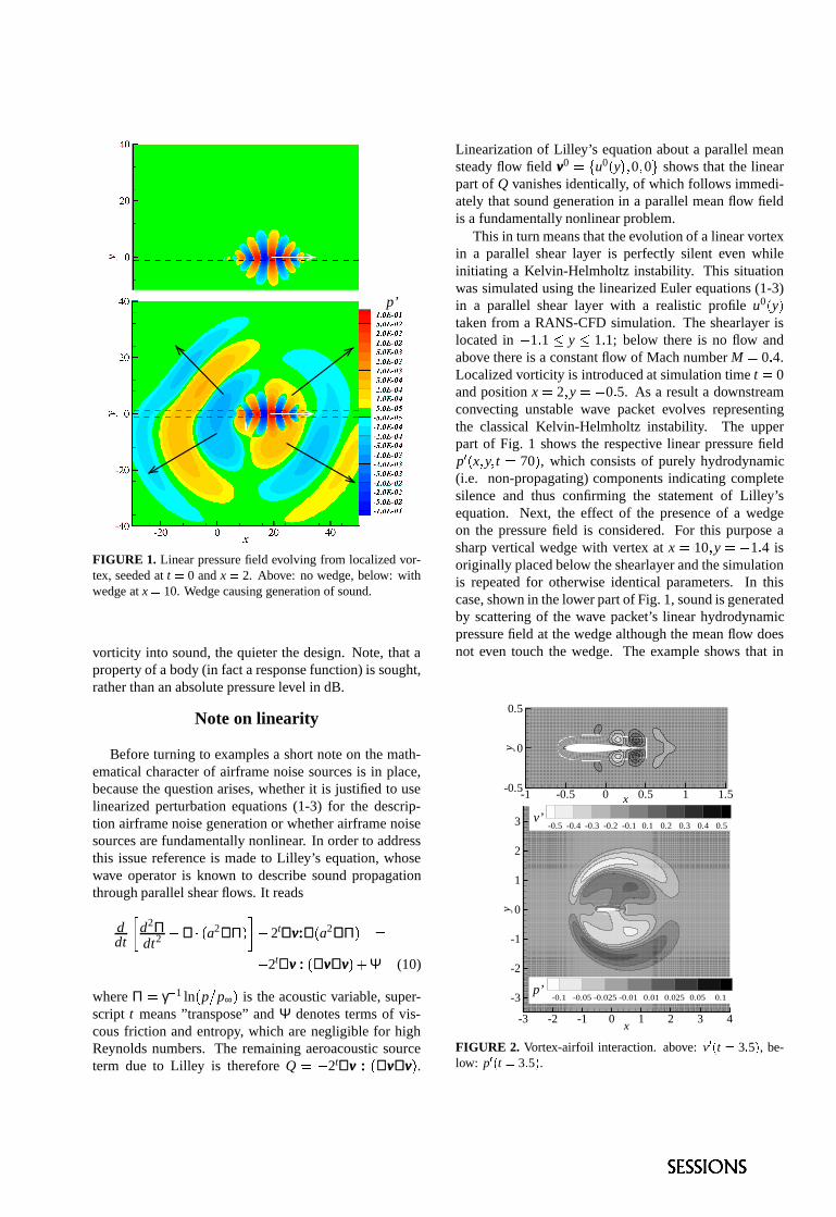
FIGURE 3. Radiated pressure from airfoils of different thick-ness in Mach-0.5 flow, referenced to free field impedance.Above: Sr=1, Below: Sr=3; Bandwidth ∆Sr U 0 V 2; [6].

lower part of the figure depicts the acoustic pressure prop-agating away from the airfoil.

At DLR, a first CAA-design study on the influ-ence of airfoil thickness on the sound generation in”dirty” inflow conditions was carried out in threedimensions[6]. Joukowski-airfoils (span along z-direction, flow along x) with different thicknesseswere subjected to the same localized test vortices withvvv F G t H 0 IWHXG y J'N x J 0 I exp M&N ln G 2 I.G x2 O y2 O z2 IYP 0 L 12 Q .Pressure time histories p FZG t I in the z H 0-plane ona circle with a radius of 1.5 chord lengths l aroundthe airfoil nose were Fourier-transformed. The Fig.3shows radiation directivities for two Strouhal numbersSr H f l P U∞ with frequency f referenced w.r.t. thefreestream velocity U∞. The transformed pressure isrelated to the maximum initial perturbation velocityv Fmax and thus appears formally as an impedance. Thediagrams show that under the same inflow conditionsthick airfoils are much quieter than thin airfoils.

CONCLUSIONS

Inviscid perturbation equations may be used tosimulate the generation mechanism of airframe noiseemploying high resolution CAA codes. Essential partof airframe noise generation rests on linear dynam-ics. The presented ”vortex-test” serves as a methodto support low-noise design of airframe componentstheoretically/numerically.

ACKNOWLEDGMENTS

Part of the work, leading to the present paper wassponsored by Deutsche Forschungsgemeinschaft DFGas part of the SWING+ project, which is gratefullyacknowledged.

REFERENCES

1. Delfs, J.W., AIAA Paper No. 2001-2199 (2001).

2. Dobrzynski, W.; Nagakura, K.; Gehlhar, B.; Buschbaum,A., AIAA Paper No. 98-2337 (1998).

3. Michel, U.; Helbig, J.; Barsikow, B.; Hellmig, M., AIAAPaper No. 98-2336 (1998).

4. Tam, C.K.W.; Dong, Z., Theoret. Comput. Fluid Dynamics,Vol.6, pp. 303–322, (1994).

5. Tam, C.K.W.; Shen, H., AIAA Paper No. 93-4325 (1993)

6. Grogger, H.A.; Lummer, M.; Lauke, Th., AIAA Paper No.2001-2137 (2001).

7. Tam, C.K.W.; Dong, Z., Journal of Computational Acous-tics, Vol.89, pp. 439–461 (1993).

������������� �������������������������������� !�"#�������$�%'&(��)���&*���� ��+�����,�

-$.0/�13254547698+:;.0<�45=?>A@CBD>E47FG8�-$.0/H=3IJ>K6L13M�NPOQ.0RJSUTHV>WEXZY�[]\7X9^`_7acbed7[]fhg5b�XZiKjlk m�^onCkqp$Wlrspst�uvuxwzyci|{`_7az} X�WEXZY�[]\�~z} X+�xX3j|�vacY��E���v�c�ziG�zyx�c�e�U{`_5b�}�} �qWEX��xX��ci|mC\�~cY�_ZX

�s�������x�0�����v��� �z�������x�7��� �����z�������Z�D�7� �z���c�3�c�5�7�v�c���z�����7� ���q�D�7�����c��� �¡�z�¡�7¢������ �7���5�0� �c� ����� �D�7� �z�H�c£J�7¢����c���z�����7� ��¤���� �¡�x¥���z� �e� ��¦��7¢��0�������7� �z�e¥����z�����7������� ��� �0§J� �e� �5��¨�©x�7�zªv���+� «x���D�7� �z����¬,­J� �7���5���c���z�����7� � � �c� ����� �D�7� �z�#� �"���v�5��¥���� ®G�5��£����G�7�x�z�E�7�� �e�v�����7� ¦v�D�7�?���z� ���9¦z�����5�Z�D�7� �z�������Z¢��c��� ������¬E¯E���s� �s� �s«x��� �7�9�5°���������� �v�3£��c�s±�� ®`�s�c£|���Z�c�5�7� � �c�l� �x�7�5�7�����`®`� �7¢q¢�� ¦z¢q�s�5¥����z� ����e���U���5�7�²�c��� �c£ �7�������e���5�Z�D�7�?³q�c�Z¢��e���U���5�7��¬K´µ� �¶�c�x¥¶����¦z� �����5�7� ��¦����7�z��� ������·��z��� ¥0�7¢��J�7� ���5¨µ���������������x�E±�� ®�¤���� �0� �c����9���5�7�5�7��� ��� �C¬K¸¹�"� �e�v�����7� ¦v�D�7�J�7¢��J���z�����¶¤���� �0� �0�7¢�� �²� �c���z·��+¢x¥����7� �¶���5�7¢��e�¶� �²�7� «x��� �7� �C¬K´º�`���z����� ���7�`� �q�������D�Z�D�7� ��¦U�7¢�����7� �D�7�����x�7�`�c£A���z�����q¦z�����5�Z�D�7� �z�,�c���q�c£A���z�����q���7�z���c¦v�D�7� �z�»·»�c���q� �c�����?�z�c� � ���D�7� �q����� ��¦0�U�7�5£��5�7�������+���z� ���7� �z���z���Z�c� ��� ��x¥ ��� �7���5�`� �c� ����� �D�7� �z�»¬`©e�z���s�7������� �7�s�c£l�7¢��?¼E���x���7�?½s���z�����7� «x���J¦c�7�z�����D�7�9���7� �5±�¥0���7�������x�7� �C¬

¾�¿qÀ#Á ÂJÃ�ÄÆÅÇ¿0ÈÊÉ#Ã�À�ËÌ;ÍvÎ�Ï;ÐeÑ»Ò�ÓxÎ�Ï;ÔDÕ�Ò�ÖqÎ"× Ø�Ù»ÚcÛ�Ü�ÝhÕ�Þ¶Ì?ßCßCÞ5Õ�ßCÞ5à�Ðxá5Ö

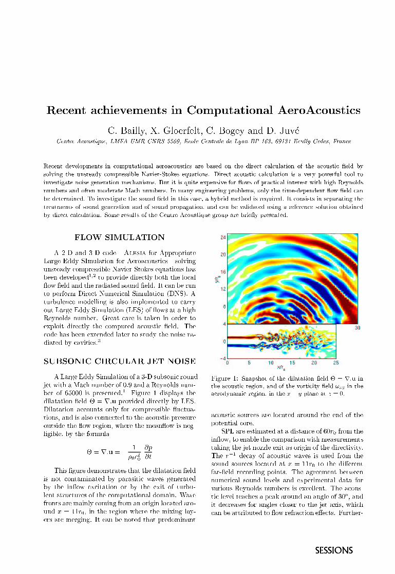
â ÐeÞ5ã�Ö0äsÒCÒ�å#æ�ç�è0éCê�Ðxá5à Õ�Ñ�ÝhÕ�Þ"Ì?ÖcÞ5Õ�Ð�ÔDÕ�é»ë7á5à�Ôcë9Î9ëZÕ�ê ì�à ÑCãéCÑ»ë7á5ÖzÐ�Ò�å,ÔDÕ�èqßCÞ5Özë5ëZà íCê Ö"î+Ðvì�à ÖcÞZÎ7æ�á5Õ�ï�ÖzësÖzð�é»Ðxá5à Õ�Ñ»ëJñ»Ð�ëí¹ÖcÖcÑ,Ò�Öcì�Öcê Õ�ß¹ÖzÒ¹ò5ó ôJá5Õ¶ßCÞ5Õxì�à�Ò�Ö?Ò�à Þ5ÖzÔ á5ê å í¹Õeá5ñ�á5ñCÖ+ê Õ�ÔcÐeêõ Õxö�÷»Öcê�Ò0ÐeÑ»Ò�á5ñCÖ3Þ�Ð�Ò�à�Ðxá5ÖzÒ¶ëZÕ�éCÑ»Ò�÷»Öcê�Ò|øEç�á²ÔcÐeѶí¹ÖJÞ5éCÑá5Õ�ß¹ÖcÞZÝhÕ�Þ5èùÏ+à Þ5ÖzÔ á�î?éCèqÖcÞ5à�ÔcÐeê`æ�à è0éCê�Ðxá5à Õ�ÑûúºÏUîUæCü øKÌá5éCÞ5íCéCê ÖcÑ»ÔDÖ�èqÕ�Ò�Öcê ê à ÑCã�à�ë¶Ðeê�ëZÕýà èqßCê ÖcèqÖcÑ�á5ÖzÒ¡á5ÕÊÔcÐeÞ5Þ5åÕ�é�á â ÐeÞ5ã�Ö9äsÒCÒ�åqæ�à è0éCê�Ðxá5à Õ�ÑÊú â ä3æCüEÕeÝ õ Õxö?ë²ÐxásÐ�ñCà ã�ñþ Öcå�ÑCÕ�ê�ÒCë"Ñ�éCè0í¹ÖcÞzø,ÿUÞ5ÖzÐxá0ÔcÐeÞ5Ö à�ë"á�Ðeï�ÖcÑ¡à Ñ�Õ�Þ�Ò�ÖcÞ"á5ÕÖ���ßCê Õ�à á�Ò�à Þ5ÖzÔ á5ê å á5ñCÖÊÔDÕ�èqßCé�á5ÖzÒ�Ð�ÔDÕ�é»ë7á5à�Ô�÷»Öcê�Ò|ø��JñCÖÔDÕ�Ò�ÖUñ»Ð�ë3í¹ÖcÖcÑ�Ö���á5ÖcÑ»Ò�ÖzÒ�ê�Ðxá5ÖcÞ3á5Õqë7á5é»Ò�å�á5ñCÖ"ÑCÕ�à�ëZÖUÞ�ÐxÎÒ�à�Ðxá5ÖzÒ�í�å,ÔcÐvì�à á5à Özëcø �

Â9Å���Â+À�Ë Ã���¡Ã����ÅÇ¿0È�� ���É�Ë�ÀHÃ�Â��Ì â ÐeÞ5ã�Ö²äsÒCÒ�å"æ�à è0éCê�Ðxá5à Õ�Ñ"ÕeÝCÐ9ÓxÎ�ÏHëZéCí»ëZÕ�ÑCà�ÔEÞ5Õ�éCÑ»Ò

� ÖDá²ö9à á5ñqÐ��ÊÐ�Ô�ñ0Ñ�éCè0í¹ÖcÞGÕeÝ��Cø �UÐeÑ»Ò0Ð þ Öcå�ÑCÕ�ê�ÒCëGÑ�éCè Îí¹ÖcÞ�ÕeÝ�����������à�ëqßCÞ5ÖzëZÖcÑ�á5ÖzÒ|ø ò��Eà ã�éCÞ5Ö��ýÒ�à�ëZßCê�Ðvå�ë0á5ñCÖÒ�à ê�Ðxá�Ðxá5à Õ�Ñ�÷»Öcê�Ò! #"#$&% 'HßCÞ5Õxì�à�Ò�ÖzÒýÒ�à Þ5ÖzÔ á5ê å,í�å â ä3æløÏ+à ê�Ðxá�Ðxá5à Õ�Ñ�Ð�ÔcÔDÕ�éCÑ�á�ë Õ�ÑCê å ÝhÕ�Þ�ÔDÕ�èqßCÞ5Özë5ëZà íCê Ö õ é»Ô á5é»ÐxÎá5à Õ�Ñ»ë)(�ÐeÑ»Òqà�ë`Ðeê�ëZÕ¶ÔDÕ�ÑCÑCÖzÔ á5ÖzÒ0á5Õ�á5ñCÖ+Ð�ÔDÕ�é»ë7á5à�ÔJßCÞ5Özë5ëZéCÞ5ÖÕ�é�á�ëZà�Ò�ÖUá5ñCÖ õ ÕxöÇÞ5Öcã�à Õ�Ñ*(�ö9ñCÖcÞ5Ö+á5ñCÖ"èqÖzÐeÑ õ ÕxöÇà�ëJÑCÖcãeÎê à ã�à íCê Ö�(Cí�å�á5ñCÖ"ÝhÕ�Þ5è0éCê�Ð

+"+$&% '!"-, �.�/10 ô/

2�3254

�JñCà�ël÷»ã�éCÞ5Ö`Ò�ÖcèqÕ�Ñ»ë7á5Þ�Ðxá5Özëlá5ñ»ÐxáKá5ñCÖ3Ò�à ê�Ðxá�Ðxá5à Õ�ÑU÷»Öcê�Òà�ë�ÑCÕeá�ÔDÕ�Ñ�á�Ðeèqà Ñ»Ðxá5ÖzÒûí�å�ß»ÐeÞ�Ð�ëZà á5à�Ô�öJÐvì�Özëqã�ÖcÑCÖcÞ�Ðxá5ÖzÒí�å�á5ñCÖ¡à Ñ õ ÕxöùÖ��CÔDà á�Ðxá5à Õ�Ñ Õ�Þ�í�åûá5ñCÖ�Ö���à áýÕeÝ�á5éCÞ5íCé�Îê ÖcÑ�á9ë7á5Þ5é»Ô á5éCÞ5Özë3ÕeÝKá5ñCÖ"ÔDÕ�èqßCé�á�Ðxá5à Õ�Ñ»ÐeêlÒ�Õ�è�Ðeà ÑKø76�Ðvì�ÖÝhÞ5Õ�Ñ�á�ëEÐeÞ5Ö`è�Ðeà ÑCê å�ÔDÕ�èqà ÑCã9ÝhÞ5Õ�è�ÐeѶÕ�Þ5à ã�à Ñ�ê Õ�ÔcÐxá5ÖzÒ¶ÐeÞ5ÕeÎéCÑ»Ò98�":���); / (Kà ÑÊá5ñCÖqÞ5Öcã�à Õ�Ñ�ö9ñCÖcÞ5Ö0á5ñCÖqèqà ��à ÑCã�ê�Ðvå�ÎÖcÞ�ë?ÐeÞ5Ö�èqÖcÞ5ã�à ÑCã»ø`ç�áUÔcÐeÑ�í¹Ö¶ÑCÕeá5ÖzÒ,á5ñ»Ðxá+ßCÞ5ÖzÒ�Õ�èqà Ñ»ÐeÑ�á

�Eà ã�éCÞ5Ö&��< ©e���c����¢��c�J�c£A�7¢��U��� � �D�Z�D�7� �z�,¤���� �&=�>�?A@ B#� ��7¢��9�c���z�����7� �3�7��¦z� �z�»·��c���¶�c£¹�7¢��J�v�c���7� ��� �µ¥�¤���� �DC*EGF9� �0�7¢���c�5�7�e�e¥����c��� �J�7��¦z� �z�»·�� �0�7¢��IH�JLK¶��� �c���?�D��MN>POe¬

Ð�ÔDÕ�é»ë7á5à�Ô ëZÕ�éCÞ�ÔDÖzëUÐeÞ5Ö0ê Õ�ÔcÐxá5ÖzÒ#ÐeÞ5Õ�éCÑ»Ò�á5ñCÖ ÖcÑ»Ò#ÕeÝ`á5ñCÖß¹Õeá5ÖcÑ�á5à�ÐeêAÔDÕ�Þ5Ö�øæ�Q â ÐeÞ5ÖsÖzë7á5à è�Ðxá5ÖzÒ Ðxá²ÐUÒ�à�ë7á�ÐeÑ»ÔDÖJÕeÝ5����; / ÝhÞ5Õ�è$á5ñCÖà Ñ õ ÕxöD(cá5Õ?ÖcÑ»ÐeíCê ÖGá5ñCÖsÔDÕ�èqß»ÐeÞ5à�ëZÕ�ÑUö9à á5ñ�èqÖzÐ�ëZéCÞ5ÖcèqÖcÑ�á�ë

á�Ðeï�à ÑCã"á5ñCÖ � ÖDá`ÑCÕ�R)Rcê Ö9Ö���à ásÐ�ëGÕ�Þ5à ã�à Ñ Õeݹá5ñCÖ?Ò�à Þ5ÖzÔ á5à ì�à á7å�ø�JñCÖ&;�SKò�Ò�ÖzÔcÐvå#ÕeÝ+Ð�ÔDÕ�é»ë7á5à�ÔqöJÐvì�Özë�à�ë0é»ëZÖzÒ¡ÝhÞ5Õ�è á5ñCÖëZÕ�éCѻҡëZÕ�éCÞ�ÔDÖzëUê Õ�ÔcÐxá5ÖzÒ¡ÐxáD8T"U���); / á5Õ�á5ñCÖ�Ò�à VlÖcÞ5ÖcÑ�áݺÐeÞZε÷»Öcê�Ò¡Þ5ÖzÔDÕ�Þ�Ò�à ÑCã�ß¹Õ�à Ñ�á�ëcø&�JñCÖ�Ðeã�Þ5ÖcÖcèqÖcÑ�á�í¹ÖDá7ö3ÖcÖcÑÑ�éCèqÖcÞ5à�ÔcÐeê+ëZÕ�éCÑ»Òûê Öcì�Öcê�ë�ÐeÑ»ÒûÖ���ß¹ÖcÞ5à èqÖcÑ�á�Ðeê+ÒCÐxá�СÝhÕ�ÞìxÐeÞ5à Õ�é»ë þ Öcå�ÑCÕ�ê�ÒCë+Ñ�éCè0í¹ÖcÞ�ë+à�ë+Ö��CÔDÖcê ê ÖcÑ�ázø��JñCÖ Ð�ÔDÕ�é»ë7Îá5à�Ô+ê Öcì�Öcê»Þ5ÖzÐ�Ô�ñCÖzësж߹ÖzÐeïqÐeÞ5Õ�éCÑ»Ò�ÐeÑ�ÐeÑCã�ê Ö+ÕeÝAÓ���W�(�ÐeÑ»Òà á¶Ò�ÖzÔDÞ5ÖzÐ�ëZÖzë?ÝhÕ�Þ"ÐeÑCã�ê Özë"ÔDê Õ�ëZÖcÞ+á5Õ,á5ñCÖ � ÖDá¶ÐX��à�ë)(|ö9ñCà�Ô�ñÔcÐeÑ0í¹ÖJÐxáZá5Þ5à íCé�á5ÖzÒ�á5Õ õ Õxö Þ5ÖDÝhÞ�Ð�Ô á5à Õ�Ñ�Ö�VlÖzÔ á�ëcø7�CéCÞZá5ñCÖcÞZÎ

èqÕ�Þ5Ö�(¹á5ñCÖ�Ð�ÔDÕ�é»ë7á5à�Ô¶Þ�Ð�Ò�à�Ðxá5à Õ�ÑÊà�ëUè0é»Ô�ñ#èqÕ�Þ5Ö è�ÐeÞ5ï�ÖzÒà Ñ á5ñCÖýÒ�Õxö9Ñ»ë7á5ÖzÐeè Ò�à Þ5ÖzÔ á5à Õ�Ñ*(²ö9à á5ñHéCß»ë7á5Þ5ÖzÐeèPëZÕ�éCÑ»Òê Öcì�Öcê�ë�Ðxá�ê ÖzÐ�ë7á �1�¡Ò � à Ñ�ÝhÖcÞ5à Õ�Þqá5Õ¡á5ñCÖýñCà ã�ñCÖzë7á�ìxÐeê éCÖÕ�í�á�Ðeà ÑCÖzÒ�Ò�Õxö9Ñ»ë7á5Þ5ÖzÐeèýø

0 30 60 90 120102

106

110

114

118

θ(deg)

SP

L(dB

)

�Eà ã�éCÞ5Ö,Í�< ©e�z�����,���7���������7�¶� ���v���G�c�?£������5�7� �z�ý�c£3�c��¦z� ������ �c�����7� ��£ �7�z� �7¢������5���D°�� ��·G�D���1O��¶£ �7�z� �7¢������5������ 5¨ �� �z¬��|°����5�7� �����x�Z�c�¹���D�Z�U�x¥����+·�³ �z� � �c¨�¼E¢��7� ���7��������� XZ[`~z} ������ ������! �·#"»����¢ �����%$�� ���'&²·�©x���7�z�U���5�7¦ XZ[²~z} � �����%$� �Z¬

Ë�ÀHÃ�Â�� �È)(�Ã�ÈÊÉ9�*( �,+ ÈÂ9Å���Â+À�Ë Ã�����È.-ÇÃ�É/+

�JñCÖqÐ�ÔDÕ�é»ë7á5à�Ô¶÷»Öcê�Ò#ã�ÖcÑCÖcÞ�Ðxá5ÖzÒ�í�åýá5ñCÖ õ Õxö Õxì�ÖcÞ"ÐÍvÎ�ÏùÔcÐvì�à á7åHà�ë�à Ñ�ì�Özë7á5à ã�Ðxá5ÖzÒHé»ëZà ÑCã�á7ö3Õ Ò�à VlÖcÞ5ÖcÑ�á,ÐeÑ»ÒÔDÕ�èqßCê ÖcèqÖcÑ�á�ÐeÞ5å�èqÖDá5ñCÕ�ÒCë)<¡ÐHÒ�à Þ5ÖzÔ á,Ñ�éCèqÖcÞ5à�ÔcÐeê+ëZà è ÎéCê�Ðxá5à Õ�Ñ Ðeѻҡà Ñ�á5Öcã�Þ�Ðeê²èqÖDá5ñCÕ�ÒCë�í»Ð�ëZÖzÒ¡Õ�Ñ¡á5ñCÖ �AÝhÕxöJÔcë6�à ê ê à�Ðeè�ë?ÐeÑ»Ò10+Ðvö9ï�à ÑCã�ë3Özð�é»Ðxá5à Õ�ÑKø6¡Ö¡Þ5ÖcßCÞ5Õ�Ò�é»ÔDÖ¡Ñ�éCèqÖcÞ5à�ÔcÐeê ê å32"Þ5à�ëZñCÑ»Ðeè0éCÞZá7å54 ë�Ö���Î

ß¹ÖcÞ5à èqÖcÑ�á�ú �1������ü,ö9à á5ñ$á5ñCÖHë5ÐeèqÖHÒ�à èqÖcÑ»ëZà Õ�Ñ»ëÊÐ�ëýà Ñá5ñCÖ#Ö���ß¹ÖcÞ5à èqÖcÑ�ázø-�JñCÖ#Ð�ÔDÕ�é»ë7á5à�Ôý÷»Öcê�ÒCë�ö3ÖcÞ5Ö�à Ñ�ì�Özë7á5à Îã�Ðxá5ÖzÒÊí�å�èqÖzÐeÑ»ëUÕeÝJæ�Ô�ñCê à ÖcÞ5ÖcÑ#Õ�í»ëZÖcÞ5ìxÐxá5à Õ�Ñ»ë)(¹à Ñ�á5ÖcÞZÝhÖcÞZÎÕ�èqÖDá5Þ5å�(�ÐeÑ»Ò ñCÕeáZÎ�ö9à Þ5Ö9ÐeÑCÖcèqÕ�èqÖDá5ÖcÞzø 6¡Ö9ßCÞ5ÖzëZÖcÑ�á`ñCÖcÞ5Öá5ñCÖJëZà è0éCê�Ðxá5à Õ�Ñ�ÕeÝ�á5ñCÖJÔcÐ�ëZÖ`ö9ñCÖcÞ5Ö`á5ñCÖ3ê ÖcÑCãeá5ñ�εá5ÕeÎ�Ò�Öcß�á5ñÞ�Ðxá5à Õ�à�ë�Í¡ú76#" ��% ��8,èqè ÐeÑ»Ò,9 "QÍ�% ��:,èqè�ü ø �JñCÖí¹Õ�éCÑ»ÒCÐeÞ5å�ê�Ðvå�ÖcÞ�ÐeñCÖzÐ�ÒÊÕeÝsá5ñCÖ�ÔcÐvì�à á7åýà�ë"ê�Ðeèqà Ñ»ÐeÞ¶ÐeÑ»Òá5ñCÖ0ÝhÞ5ÖcÖzë7á5Þ5ÖzÐeè��ÊÐ�Ô�ñÊÑ�éCè0í¹ÖcÞ"à�ë �Cø ;�ø��JñCÖ þ Öcå�ÑCÕ�ê�ÒCëÑ�éCè0í¹ÖcÞ9í»Ð�ëZÖzÒ,Õ�Ñ�á5ñCÖ¶ÔcÐvì�à á7å�Ò�Öcß�á5ñýà�ë þ Ö�<�"): �1�����Cø�JñCÖ,à ÑCà á5à�Ðeê3í¹Õ�éCÑ»ÒCÐeÞ5å�ê�Ðvå�ÖcÞ�á5ñCà�Ô�ï�ÑCÖzë5ë0Ðxá0á5ñCÖýÔcÐvì�à á7åê ÖzÐ�Ò�à ÑCãqÖzÒ�ã�Ö�à�ë�= /?> � % Í@9*A�à á+ÔDÕ�Þ5Þ5ÖzëZß¹Õ�Ñ»ÒCësá5Õ�Ð Þ�Ðxá5à Õ6CB�=�D > ��� (�ö9ñCÖcÞ5Ö�=�DUà�ëJá5ñCÖ�èqÕ�èqÖcÑ�á5éCèoá5ñCà�Ô�ï�ÑCÖzë5ëcø�JñCÖsÔ�ñCÕ�à�ÔDÖ`ÕeÝ»Ð?ñCà ã�ñ¶ëZéCí»ëZÕ�ÑCà�Ô`ëZß¹ÖcÖzÒ�à�ëAà Ñ�á5ÖcÞ5Özë7á5à ÑCã

í¹ÖzÔcÐeé»ëZÖ"á5ñCÖ"ÝhÞ5Özð�éCÖcÑ»ÔDå,à Ñ»ÔDÞ5ÖzÐ�ëZÖzëJëZê à ã�ñ�á5ê å�ö9à á5ñ �ÊÐ�Ô�ñÑ�éCè0í¹ÖcÞEÐeÑ»Ò+á5ñCÖsÔcÐvì�à á7å+à�ëKÑCÕ9èqÕ�Þ5Ö`ÔDÕ�èqß»Ð�Ô áAÞ5Öcê�Ðxá5à ì�Öcê åá5Õ0á5ñCÖ"Ð�ÔDÕ�é»ë7á5à�Ô?öJÐvì�Öcê ÖcÑCãeá5ñKø ��Õ�Þ5ÖcÕxì�ÖcÞ1(eá5ñCÖ+á5Özë7á9ÔcÐ�ëZÖà�ësèqÕ�Þ5Ö+Þ5Öcê ÖcìxÐeÑ�á`ÝhÕ�Þ3à Ñ�á5Öcã�Þ�Ðeê»èqÖDá5ñCÕ�ÒCë3í¹ÖzÔcÐeé»ëZÖ+èqÖzÐeÑõ Õxö Ö�VlÖzÔ á�ë,Õ�ÑÇëZÕ�éCÑ»Ò�ßCÞ5Õ�ß»Ðeã�Ðxá5à Õ�Ñûí¹ÖzÔDÕ�èqÖ#à èqß¹Õ�ÞZÎá�ÐeÑ�ázøÌHæ�Ô�ñCê à ÖcÞ5ÖcÑ"ì�à�ëZé»Ðeê à RzÐxá5à Õ�Ñ*(zÔDÕ�Þ5Þ5ÖzëZß¹Õ�Ñ»Ò�à ÑCãJö9à á5ñ�ì�ÖcÞZÎ

á5à�ÔcÐeê¶ã�Þ�Ð�Ò�à ÖcÑ�á�ë�ÕeÝ�Ò�ÖcÑ»ëZà á7å�(�ëZñCÕxö?ë�á5ñCÖHë7á5Þ5é»Ô á5éCÞ5Ö�ÕeÝ

á5ñCÖ¡Þ�Ð�Ò�à�Ðxá5ÖzÒ�÷»Öcê�ÒÇà ÑÇ÷»ã�éCÞ5Ö¡Ó»úºÐ�ü ø �Jö3Õ�öJÐvì�ÖÊß»ÐxáZÎá5ÖcÞ5Ñ»ë�ÐeÞ5Ö,ì�à�ëZà íCê Ö�ÝhÕ�Þ á5ñCÖýß¹Õ�ëZà á5à ì�Öýã�Þ�Ð�Ò�à ÖcÑ�á�ë�úºÒCÐeÞ5ïCüG(ö9ñCà�Ô�ñ à Ñ�á5ÖcÞZÝhÖcÞ�á5Õ�ã�ÖDá5ñCÖcÞ0Ò�éCÞ5à ÑCã�ßCÞ5Õ�ß»Ðeã�Ðxá5à Õ�ÑKø&�JñCÖcà Þë7á5Þ5Õ�ÑCã0éCß»ë7á5Þ5ÖzÐeèoÒ�à Þ5ÖzÔ á5à ì�à á7å�à�ëJÔ�ñ»ÐeÞ�Ð�Ô á5ÖcÞ5à�ë7á5à�Ô9ÕeÝAñCà ã�ñëZß¹ÖcÖzÒ ÔDÕ�Ñ�ì�ÖzÔ á5à Õ�Ñ$í�å á5ñCÖHÝhÞ5ÖcÖûë7á5Þ5ÖzÐeèýø �JñCÖzëZÖHÞ�ÐxÎÒ�à�Ðxá5à Õ�Ñ»ë�ÐeÞ5Öýà Ñ�ð�é»Ðeê à á�Ðxá5à ì�Öcê åHã�Õ�Õ�ÒûÐeã�Þ5ÖcÖcèqÖcÑ�áqö9à á5ñá5ñCÖ�æ�Ô�ñCê à ÖcÞ5ÖcÑHßCà�Ô á5éCÞ5Ö,ÕeÝE2"Þ5à�ëZñCÑ»Ðeè0éCÞZá7åûú]÷»ã»ø�Ó»úhí¹üZü ø�JñCÖ9Ö���ß¹ÖcÞ5à èqÖcÑ�á�Ðeê¹æ�á5Þ5Õ�éCñ»Ðeê�Ñ�éCè0í¹ÖcÞ`ÕeÝlÕ�ë5ÔDà ê ê�Ðxá5à Õ�Ñ»ëGà�ëæ�á�"�� % ; ��(CÔDÕ�Þ5Þ5ÖzëZß¹Õ�Ñ»Ò�à ÑCã¶á5Õ�ÐeÑ�ÖcÞ5Þ5Õ�ÞJÕeÝ �!F ö9à á5ñ�á5ñCÖÝhÞ5Özð�éCÖcÑ»ÔDåûÝhÕ�éCÑ»ÒÇà ÑÇÕ�éCÞ�ëZà è0éCê�Ðxá5à Õ�ÑKø �JñCÖ þ Õ�ë5ëZà á5ÖcÞëZÖcèqà Î�ÖcèqßCà Þ5à�ÔcÐeêJÝhÕ�Þ5è0éCê�СßCÞ5Õxì�à�Ò�Özë�æ�á�" � % ; ��ÝhÕ�Þqá5ñCà�ëÔDÕ�Ñ�÷»ã�éCÞ�Ðxá5à Õ�Ñ,ö9à á5ñ�á7ö3Õqì�Õ�ÞZá5à�ÔDÖzë3à Ñ�á5ñCÖ¶ëZñCÖzÐeÞ9ê�Ðvå�ÖcÞzø

úºÐ�ü úhí¹ü�Eà ã�éCÞ5ÖUÓ < ©e�Z¢�� � �5�7���¶��� �5�7���7���G���c���7�������z����� ��¦?�7�9���Z�c�����v�5��¨�7�c�»���5�7� �z�D�7� �v�s�c£»�7¢��3��������� �µ¥�� � �%�K���7�������x�G��� �U��� �D�7� �z�»· � �G�HJ�7� ��¢����c�U�����µ¥�I �G�5°����5�7� �����x� �����%J�J �Z¬

È��LK!Ë�À#Á�¿A�*(NM���Ä ��Ë!É ÂO Õ�èqßCé�á5à ÑCã9á5à èqÖ`öJÐ�ë|ßCÞ5Õxì�à�Ò�ÖzÒUí�åUç�Ñ»ë7á5à á5é�áGÒ�é0Ï*PÖDÎ

ì�Öcê Õ�ßCß¹ÖcèqÖcÑ�á`ÖDásÒ�Özë þ Özë5ëZÕ�éCÞ�ÔDÖzëEÖcÑqç�Ñ�ÝhÕ�Þ5è�Ðxá5à�ð�éCÖ?æ�ÔDà ÎÖcÑ�á5à ÷¹ð�éCÖ�úhç7Ï þ çZæ,Î O î þ æCü ø

���¾ � ���Ë-�!�#ÂQ�RTSVUXW�Y'Z![E\]Z@R_^V` a�abY'Z![E\@c)d@e#fEgWVZ@h�\ ·�i)O1O1Oe·v§3�����5�7� � �c���� �U��� �D�7� �z�¶�c£¹�7¢��s���z������¦z�����5�Z�D�7� �¶�x¥��v�c���7�5°����c� �7� ��¦� �"�s��� °�� ��¦s� ��¥x�5� ·�j_k�jTjml%n@o�prqGs�t]·@u#v ��� i��Z·wi�i � OD¨�i�i ��x ¬

yzRTSVUXW�Y'Z#[E\]ZwR_^V` a�abY'Z#[E\wc)d@e#fEgWVZwh�\ ·@i)O1O1Oe·�¼E�z�������Z�D¨�7� �z�q�c£|�7¢��9���z�����0�Z�z��� �D�7� � �x¥ ��{D¨º­L���5�s����� ��¦|"¹�D�7¦z��A���e¥q©e� �U��� �D�7� �z�»·�½s´�½3½~}|�c���5�Ci)O1O1OD¨�i)O1O � ¬

��Ea�SVWw�G��Wwa���Zw�|\]ZwR_^V` a�abY'Z![E\wc)d@e#fEgWVZwh�\ ·�i)O1O � ·e¼E�z�"¨�����Z�D�7� �z���c£E�7¢��+���z� ���+�Z�z��� �D�7� ���x¥��¶���������z��� �U� � �e� �µ¥����� ��¦"��� �7���5�`��� �U��� �D�7� �z� �c��� �c���z�����7� �9�c���c� �z¦c¥x·�½s´�½3½}|�c���5�Ci)O1O � ¨�i�i�i�e¬

��R_^V` a�abY'Z?[E\]ZERTSVUXW�Y'Z?[E\�c�d@e#fEgWVZ�h�\ ·Ci)O1O1Oe·9§3�z� ������z�������Z�D�7� �z�¡����� ��¦����z���7���q�7�5�7���¶� �¡�7¢��."»� ��� �D�7� �� ��K��� �5�"� «x���D�7� �z����·E½s´�½3½�}|�c���5�|i)O1O1OD¨�i)O� $ ·²�c���������7� �� ��j_k�jTj�l%n@o�prqGs�t]¬

The Role of Computational Aeroacoustics in ThermoacousticsP. J. Morrisa and S. Boluriaana

aDepartment of Aerospace Engineering, Penn State University, University Park, PA 16802, USA

Thermoacoustic devices use the phase relationship between the pressure and particle velocity in the Stokes boundary layer nearsurfaces to transport heat from cold to hot heat exchangers. For thermoacoustic devices to be optimized, an improved understandingof unsteady minor losses is required. In this paper a parallel numerical simulation of the minor losses in a sudden expansion in aresonator is described. The Navier-Stokes equations are discretized in space and time with high-order accurate numerical schemes.These schemes, that are also used in computational aeroacoustics, minimize numerical dispersion and dissipation errors. A highamplitude standing wave is generated in a resonator with a sudden change in cross-sectional area. The details of the unsteady flow inthe vicinity of the sudden expansion are provided. It is shown that mean recirculating flow regions are established in the two sections ofthe resonator. The average pressure losses across the expansion are determined and the relative contributions of the Bernoulli pressureand the total pressure losses due to the generation of vorticity are estimated.

INTRODUCTION

Thermoacoustic devices can be either prime movers orheat pumps. Swift [1] provides a description of the basicphysical processes involved as well as examples of dif-ferent thermoacoustic engines. Recently built thermoa-coustic engines, such as the Stirling heat engine designedby Backhaus and Swift [2], have efficiencies that rival thecommon internal combustion engine. This is achievedthrough the use of a traveling acoustic wave, that has thecorrect pressure/volume phasing of the Stirling cycle, inone part of the engine. This wave is maintained at a highamplitude by a standing wave in another section of theengine. To prevent a net mean flow in the traveling waveloop of the device, that reduces the system’s efficiency, a“jet-pump” is used. The average minor losses across thejet-pump eliminate the mean flow. Minor losses are well-documented for steady flows (see Idelchik [3]): however,this is not the case for the unsteady flow in a thermoacous-tic engine. The purpose of the research described here isto address this lack of understanding.

TECHNICAL APPROACH

In order to describe the interaction between the acous-tic wave in the resonator and the resonator walls theNavier-Stokes equations are used. They are written in ageneralized coordinate system. The total energy equationis used as well as the equation of state for a perfect gas.The coefficient of viscosity is related to the thermody-namic properties using Sutherland’s formula. A Prandtlnumber of 0.72 is used to relate the coefficients of viscos-ity and thermal conductivity. No turbulence model is usedin the present simulations. The equations are discretizedusing the Dispersion Relation Preserving algorithm ofTam and Webb [4] in space and a fourth-order Runge-Kutta scheme in time. The computer code is written in

Fortran 90 with the Message Passing Interface (MPI) asthe parallel implementation. A domain decompositionmethod is used, in which the physical domain is decom-posed into sub-domains and message passing is only em-ployed at the sub-domain boundaries. In addition, a par-allel multiblock grid structure is used. This is appropriatefor the present problem of a resonator with two sectionsof different cross sections. The geometry and computa-tional domain used in the present two-dimensional sim-ulations are shown in Fig. 1. The lengths are nondimen-sionalized by the length of the larger resonator. Differ-ent blocks are used for the grids in the two parts of theresonator in order to insure the grid orthogonality. The

1.0

0.5

0.03

0.05

Line Source

0.025

0.025A

0.003

B

y

x

FIGURE 1. Sketch of the computational domain. Not to scale.

calculations are performed on a PC cluster. The compu-tational time on 32 processors is 2.8µsec/grid point/timestep. A companion experimental resonator (see Doller etal. [5]) is driven by either a shaker or a loudspeaker. Inorder to model the effect of the driver, a source term isintroduced into the continuity equation. It has a Gaussiandistribution in the x-direction and is located a distance of0.05 from the closed end of the larger channel, as shownin Fig. 1. A source term is also introduced into the energyequation to insure that only acoustic disturbances are gen-erated. No slip and no penetration conditions are appliedat all walls. Either adiabatic or isothermal wall boundaryconditions are enforced.

RESULTS AND DISCUSSION

After an initial transient period, a standing wave is es-tablished in the smaller resonator channel. In the com-panion experiment, the resonant frequencies are estab-lished with a broadband excitation. In the present calcu-lations, a single frequency that generates a quarter wave-length standing wave in the smaller channel is used. Mor-ris et al. [6] show how the system settles into a periodicstate after approximately twenty periods. Near the changein the cross section, there is a periodic shedding of vor-tices associated with the jet-like part of the cycle. In-stantaneous streamtraces are shown in Fig. 2. The flow issymmetric about the channel centerline. This is due to theplane wave excitation. Two pairs of vortices of equal rota-tion sense are seen. In addition, a pair of vortices with theopposite sense form in between them. The vortices moveaway from the contraction by a process of mutual induc-tion. In addition, a net mean flow is generated. Immedi-ately at the contraction there is a very small mean flowon the channel centerline towards the smaller channel.A stronger centerline mean flow away from the contrac-tion is observed in the larger channel. These mean flows

-0.03 -0.02 -0.01 0 0.01 0.02 0.030.5

0.51

0.52

0.53

0.54

0.55

0.56

0.57

0.58

0.59

FIGURE 2. Streamtraces of the instantaneous flow in the res-onator.

are associated with two recirculating regions that fill bothparts of the resonator.The instantaneous pressure differ-ence between point A in the larger channel and point Bin the smaller channel (shown in Fig. 1) reaches a steadyvalue after the transient period. This pressure differencehas contributions from the Bernoulli pressure (see Wangand Lee [7]) and losses due to the generation of vorticity.The former is a second order effect associated with thefinite amplitude of the acoustic pressure and particle ve-locity. It’s contribution is estimated to be 25% of the totalpressure difference. Thus, the larger contribution may beassociated with the generation of vorticity at the suddenexpansion/contraction.

The simulations described here represent a prelimi-nary examination of the ability of numerical simulations,based on methods from computational aeroacoustics, toaid in the understanding and optimization of fluid dy-namic phenomena in thermoacoustic devices. Much workremains to be done. In particular, more realistic three-dimensional geometries that match the actual jet pumpsshould be examined. The acoustic driver needs to bemodeled more accurately. Also, at high amplitudes, theboundary layers may be alternately laminar or turbulent.This is caused by the periodic variation of the pressuregradient from favorable to adverse. This is a very chal-lenging turbulence modeling problem. Some preliminaryefforts by the authors suggest that an unsteady Reynolds-averaged Navier-Stokes method could be useful.

ACKNOWLEDGEMENTS

This work was supported by the Office of Naval Re-search.

REFERENCES

1. G. W. Swift, Journal of the Acoustical Society of America84, 1145 (1988).

2. S. Backhaus and G. W. Swift, Nature 399, 335 (1999).

3. I. E. Idelchik, Handbook of Hydraulic Resistance, 3rd ed.(Begell House, New York, 1994).

4. C. K. W. Tam and J. C. Webb, J. Computational Physics 107,262 (1993).

5. A. Doller, A. A. Atchley, and R. Waxler, Journal of theAcoustical Society of America 108, 2569 (2000).

6. P. J. Morris, S. Boluriaan, and C. M. Shieh, Computa-tional Thermoacoustic Simulation of Minor Losses Througha Sudden Contraction and Expansion, AIAA/CEAS Paper2001/2272, 2001.

7. T. G. Wang and C. P. Lee, in Nonlinear Acoustics, edited byM. F. Hamilton and D. T. Blackstock (Academic Press, NewYork, 1998), Chap. 6, pp. 177–204.

Aeroacoustic studies and tests performed to optimizethe acoustic environment of the Ariane 5 launch vehicle

D. Gély, G. Elias and C. BressonOffice National d’Etudes et de Recherches Aérospatiales

29, avenue de la Division LeclercBP 72, 92320 Châtillon Cedex - France

To decrease the acoustic levels inside the Ariane 5 fairing and to reduce the excitation applied to the payload, it was necessary toinvestigate a method for reducing substantially the acoustic environment during the lift-off. The highest-noise radiating regions wereidentified by analyzing the signals from a microphone array implemented on the launch vehicle. It is to our knowledge the first time sucha technique is used on a launch vehicle. The MARTEL facility was then used to characterize the efficiency of a horizontally extension ofthe lateral flues. Based on test results and applying similarity criteria, it was possible to determine the length of this extension necessaryto achieve the required noise attenuation inside the fairing. The acoustic measurements made on the launch vehicle after the flueextension construction in Kourou confirmed the reduced scale predictions obtained at MARTEL facility.

INTRODUCTION

The more and more powerful launch vehicles, such as Ariane 5,involve an increase of the external Sound Pressure Level (SPL).As the confort of launch vehicle at lift-off may become a quiteimportant commercial argument for the customers in the futuretherefore, a continuous effort must be kept in order to obtain“low” acoustic levels in the payload bay. The acoustic analysesmade during the V503 qualification flight of Ariane 5 confirmedthe possibility to reduce the acoustic levels inside the fairingwhen the launch vehicle goes through the altitude from 10 to 20meters. This study has been supported by the Ariane Programand the Research & Technology program of CNES.

MEASUREMENTS DURING V503 FLIGHT

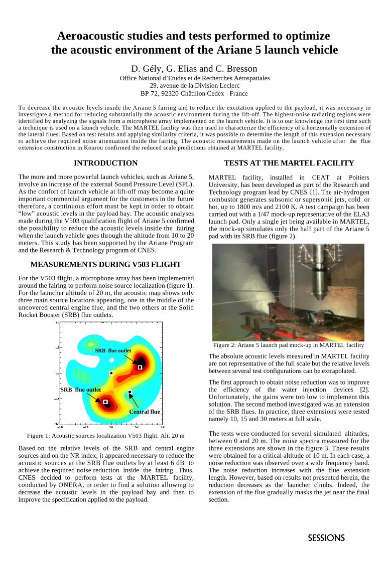
For the V503 flight, a microphone array has been implementedaround the fairing to perform noise source localization (figure 1).For the launcher altitude of 20 m, the acoustic map shows onlythree main source locations appearing, one in the middle of theuncovered central engine flue, and the two others at the SolidRocket Booster (SRB) flue outlets.

Figure 1: Acoustic sources localization V503 flight. Alt. 20 m

Based on the relative levels of the SRB and central enginesources and on the NR index, it appeared necessary to reduce theacoustic sources at the SRB flue outlets by at least 6 dB toachieve the required noise reduction inside the fairing. Thus,CNES decided to perform tests at the MARTEL facility,conducted by ONERA, in order to find a solution allowing todecrease the acoustic levels in the payload bay and then toimprove the specification applied to the payload.

TESTS AT THE MARTEL FACILITY

MARTEL facility, installed in CEAT at PoitiersUniversity, has been developed as part of the Research andTechnology program lead by CNES [1]. The air-hydrogencombustor generates subsonic or supersonic jets, cold orhot, up to 1800 m/s and 2100 K. A test campaign has beencarried out with a 1/47 mock-up representative of the ELA3launch pad. Only a single jet being available in MARTEL,the mock-up simulates only the half part of the Ariane 5pad with its SRB flue (figure 2).

Figure 2: Ariane 5 launch pad mock-up in MARTEL facility

The absolute acoustic levels measured in MARTEL facilityare not representative of the full scale but the relative levelsbetween several test configurations can be extrapolated.

The first approach to obtain noise reduction was to improvethe efficiency of the water injection devices [2].Unfortunately, the gains were too low to implement thissolution. The second method investigated was an extensionof the SRB flues. In practice, three extensions were testednamely 10, 15 and 30 meters at full scale.

The tests were conducted for several simulated altitudes,between 0 and 20 m. The noise spectra measured for thethree extensions are shown in the figure 3. These resultswere obtained for a critical altitude of 10 m. In each case, anoise reduction was observed over a wide frequency band.The noise reduction increases with the flue extensionlength. However, based on results not presented herein, thereduction decreases as the launcher climbs. Indeed, theextension of the flue gradually masks the jet near the finalsection.

SRB flue outlet

SRB flue outlet

Central flue

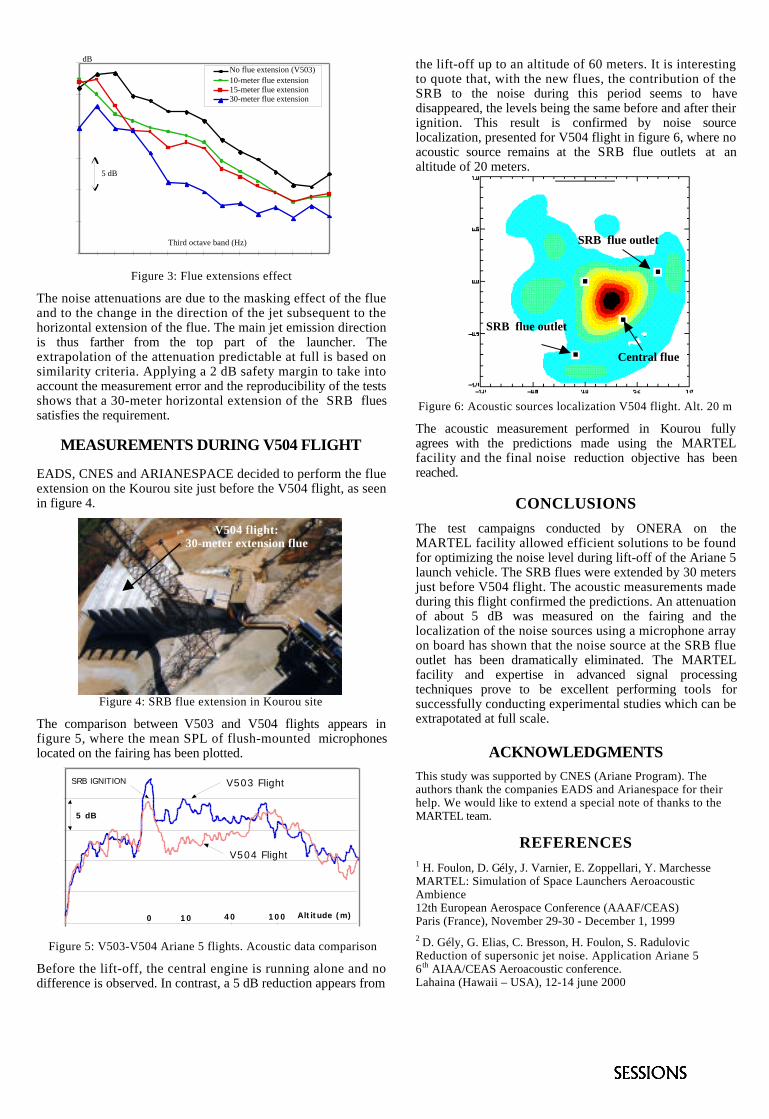
No flue extension (V503)10-meter flue extension15-meter flue extension30-meter flue extension

dB

Third octave band (Hz)

5 dB

Figure 3: Flue extensions effect

The noise attenuations are due to the masking effect of the flueand to the change in the direction of the jet subsequent to thehorizontal extension of the flue. The main jet emission directionis thus farther from the top part of the launcher. Theextrapolation of the attenuation predictable at full is based onsimilarity criteria. Applying a 2 dB safety margin to take intoaccount the measurement error and the reproducibility of the testsshows that a 30-meter horizontal extension of the SRB fluessatisfies the requirement.

MEASUREMENTS DURING V504 FLIGHT

EADS, CNES and ARIANESPACE decided to perform the flueextension on the Kourou site just before the V504 flight, as seenin figure 4.

Figure 4: SRB flue extension in Kourou site

The comparison between V503 and V504 flights appears infigure 5, where the mean SPL of flush-mounted microphoneslocated on the fairing has been plotted.

Figure 5: V503-V504 Ariane 5 flights. Acoustic data comparison

Before the lift-off, the central engine is running alone and nodifference is observed. In contrast, a 5 dB reduction appears from

the lift-off up to an altitude of 60 meters. It is interestingto quote that, with the new flues, the contribution of theSRB to the noise during this period seems to havedisappeared, the levels being the same before and after theirignition. This result is confirmed by noise sourcelocalization, presented for V504 flight in figure 6, where noacoustic source remains at the SRB flue outlets at analtitude of 20 meters.

Figure 6: Acoustic sources localization V504 flight. Alt. 20 m

The acoustic measurement performed in Kourou fullyagrees with the predictions made using the MARTELfacility and the final noise reduction objective has beenreached.

CONCLUSIONS

The test campaigns conducted by ONERA on theMARTEL facility allowed efficient solutions to be foundfor optimizing the noise level during lift-off of the Ariane 5launch vehicle. The SRB flues were extended by 30 metersjust before V504 flight. The acoustic measurements madeduring this flight confirmed the predictions. An attenuationof about 5 dB was measured on the fairing and thelocalization of the noise sources using a microphone arrayon board has shown that the noise source at the SRB flueoutlet has been dramatically eliminated. The MARTELfacility and expertise in advanced signal processingtechniques prove to be excellent performing tools forsuccessfully conducting experimental studies which can beextrapotated at full scale.

ACKNOWLEDGMENTS

This study was supported by CNES (Ariane Program). Theauthors thank the companies EADS and Arianespace for theirhelp. We would like to extend a special note of thanks to theMARTEL team.

REFERENCES1 H. Foulon, D. Gély, J. Varnier, E. Zoppellari, Y. MarchesseMARTEL: Simulation of Space Launchers AeroacousticAmbience12th European Aerospace Conference (AAAF/CEAS)Paris (France), November 29-30 - December 1, 19992 D. Gély, G. Elias, C. Bresson, H. Foulon, S. RadulovicReduction of supersonic jet noise. Application Ariane 56th AIAA/CEAS Aeroacoustic conference.Lahaina (Hawaii – USA), 12-14 june 2000

V504 flight:30-meter extension flue

SRB flue outlet

SRB flue outlet

Central flue

Altitude (m)

V503 Flight

5 dB

V504 Flight

0 10 40 100

SRB IGNITION

Influence of compartment size on radiated sound powerlevel of a centrifugal fan

Leping Feng

MWL, Department of Vehicle Engineering, KTH, SE-100 44 Stockholm, Swedene-mail: fengl@fkt.kth.se

The influence of the compartment size on the radiated sound pressure level of a centrifugal fan is investigated experimentally.The measurement set-up consists of a commercial centrifugal fan and a cavity with adjustable walls and ceiling. The inflowcondition is adjusted indirectly by adjusting the geometry of the box, in order to avoid the difficulties to describe and measurethe inflow conditions quantitatively. The tests are performed for a range of typical situations of ventilation systems. The soundpressure levels in a few typical positions are measured in a semi-aechoic room. Some useful results, and an empirical relationbetween the sound power level and the geometry of the cavity in a certain range, are obtained from the measurements.

INTRODUCTION

The radiated sound power level of a centrifugal fanis strongly influenced by the inflow condition. Anexample of this is that a fan usually radiates 3 dB ormore sound power when located inside a ventilationsystem than in a free condition. There are severaldifferent parameters that may influence the inflowconditions. In this paper, we only deal with onesituation: the change of the cross section of thecompartment where the fan is located.

DESCRIPTION OF TEST SET-UP

The tests were performed in the semi-anechoicroom of the Department, with the test set-up shown inFigure 1. The positions of the walls and roof areadjustable to make variable cross sections of the fancompartment. The centrifugal fan tested is SAMI GSwith 11 blades manufactured by ABB.

Figure 1 Illustration of the test set-up

Figure 2. Illustration of microphone positions

The opening of the outlet, which is a 0.3 X 0.3 msquare duct, is covered with a perforated panel(perforated ratio ∼ 30%) in order to make the fanworking in practical working point. Two microphonesare employed to register the sound pressure levels.One is located at the same plane of the outlet, 0.65 mfrom the centre of the duct. Another is located at thecentre line of the inlet side, 2 meters away from thecompartment (see Figure 2). The tests are performedin four different (motor) speeds: 700, 1000, 1500 and1900 rpm. Eleven cross sections of the compartment,varying from 0.22 to 0.596 m2, or from 2.443 to 6.622times of the area of the outlet duct, are tested.

SOME RESULTS

In order to check the general trend of the soundpressure/power level in function of the size of thecompartment, the registered sound pressure levels atthe four different rotating speeds are �normalised�.That is, the total sound pressure levels at differentrotating speeds are set to be equal to that of the soundpressure level when the rotating speed is 1000 rpm.The sound pressure level at each frequency band isthen calculated as

Mic. 1(outlet side)

Mic. 2(inlet side)

DuctFan

compartment

2 m

0.5 m

60

65

70

75

80

85

90

95

100 200 400 800 1600 3150 A-weghted

Frequency, Hz

outlet

inlet

Figure 3 Typical spectra at the two positions

)( 1 rkinormalisedi LLLL −+= (1)

where subscript �i� denotes 1/3 octave band number,�1k� and �r� are rotating speed.

Typical spectra of sound pressure levels measuredat the two microphone positions are shown in Figure 3.They have different shapes. The differences at lowfrequencies could be due to flow, since the flow speedat outlet side is much higher than that at inlet side. Thehigh frequency components, on the other hand, mightbe due to the interaction between the flow and theperforated panel. Since the microphone at the inletside is directly pointed to the fan and the cross sectionat this side is much larger, the signal registered bymicrophone 2 might more correctly reflect the changesof the fan due to the size change of the compartment.

The test situations of the cross section arenormalised by the area of the outlet duct in order to geta non-dimensional measure. Figure 4 & 5 shows thethird octave band sound pressure level at microphone 2as a function of the normalised area. As a generaltendency, sound pressure levels decrease when the areais increased, with the value dependent on frequencies.Results from microphone 1 show the same tendency.

65

70

75

80

85

90

2 3 4 5 6 7

Normalised area

100

125

160

200

250

315

400

500

630

Figure 4 Sound pressure levels at microphone 2as a function of area: low frequencies

65

70

75

80

85

90

95

2 3 4 5 6 7

Normalised area

800

1000

1250

1600

2000

2500

3150

4000

5000

A

Figure 5 Sound pressure levels at microphone 2as a function of area: high frequencies

In order to get a general picture of the influence ofthe cross section on the radiated sound pressure level,linear regression is made for all measured data, indecibel, according to equation

BsAL += 72 ≤≤ s (2)

where s is the normalised area and A and B regressioncoefficients. Figure 6 shows the coefficient B, which isthe increase of the sound pressure level when the sizeof the compartment increases the area of one crosssection of the outlet duct. For both microphones, thisvalue is almost always negative, indicating thatreducing the compartment size will increase soundpressure levels at all frequency bands. Although thereis a big difference for 1/3 octave band values, thecoefficient B is almost same for A-weighted soundpressure levels measured at both microphone positions.

CONCLUSIONS

Reducing cross section of the fan compartment willincrease the radiated sound power level. This increaseseems not as big as we expected.

-1.6

-1.4

-1.2

-1

-0.8

-0.6

-0.4

-0.2

0

0.2

0.4

100 200 400 800 1600 3150 A-weghted

Frequency, Hz

Figure 6 Regression coefficients BSolid: inlet side; Dotted: outlet side

Effects of Blade Material on Sound Radiation by AttachedCavity in Unsteady FlowS. Kovinskayaa and E. Amrominb

aSeagate Technology, 10323 West Reno, Oklahoma City, OK73127, USAbMechmath LLC, 2109 Windsong,Edmond,OK73034, USA

Sound radiation by a cavity attached to a blade under unsteady flow excitation is analyzed. It is shown that cavityvolume oscillations and radiated sound power are sensitive to variations in ratio of blade material Young’s modulus to product offluid density on square of flow speed. These variations change both frequencies and levels of peaks in spectra of radiated sound.

MATHEMATICAL FORMULATION OFPROBLEM

Prediction of sound radiation by cavitatingblades/hydrofoils is currently based on model tests.Because of differences between flow-induced sound inmodel and full-scale flows, extrapolations ofexperimental data to full-scale conditions are notcompletely satisfactory, especially in low-frequencyband [1]. Selection of appropriate similitude criteria is animportant problem that can be clarified by thenumerical analysis. A realistic analysis must take intoaccount simultaneous oscillations of cavity thicknessand length under periodical excitations of incomingflow, and represents a nonlinear problem with avarying boundary. Theory [2] allows such analysis forelastic blades with the use of 2-D numerical modeling.For a blade (hydrofoil) at a given time-averaged angleof attack, periodical perturbation of incoming flow canbe caused by turbulence. The perturbation magnitudesare much smaller than free-stream speed. The vibrationof blade with attached cavity in unsteady flow (Fig.1)is described in 2D approach by equation for beam inbending motion:

FUtVh

xVJiE

x 2*)1(

2

2

2

2

2

2

2�

�� ��

��

�

��

�

� (1)

Here U is free-stream speed; V is transversedisplacement of the blade; � is its loss factor; E is itsYoung’s modulus; h and J are thickness and inertiamoment of its sections; �* and � are densities of bladematerial and water; F is the hydrodynamic loadcoefficient. The coefficient F depends on velocitypotential � that is a solution of Laplace equation

0��� with the following boundary conditions:

yt

V

S �

��

�

� �

1

; yt

BV

S �

�

�

���

�

2

)( (2)-(3)

32

22)(12

SS t

FU ��

���

��

�

������

�� (4)

Here B is the cavity thickness, S1 is a cavitation-freeblade surface, S2 is the cavity surface, S3 is projectionof S2 on down surface of blade; � is potential of time-averaged flow around the blade. Cavitation number�=2�P/(�U2), where �P is a difference betweenpressure in incoming flow and within the cavity. Thesystem (1)-(4) must be completed by Joukovski-Kuttacondition that defines the blade lift. For periodicexcitations that correspond to boundary condition����xx��0 and ����yx��Aei�t (where A=const;� is excitation frequency), Eq.(1) can be rewritten as

2)1( 2

22

2

2

2 FRChVS

xViJK

xt ��

�

��

�

��

Here C is the blade’s chord (see Fig. 1); K=E/(�U2),R=�*/�, and St=�C/U are dimensionless parametersthat affect vibration.

C

L

U

a

Fig. 1. Flow around a blade section.

Mechanical boundary conditions of rigid clampingin a middle part of the blade (where V=dV/dx=0) andof free edges (where d2V/d2x=d3V/dx3=0) are sufficient

for integration of Eq. (1) and determination of bladevibration. Estimating cavitation-induced soundradiation, it is important to keep in mind that anoscillation of the cavity volume D is its principal cause,and sound power level Sp~d2D/dt2 [1]. This volume,however, depends on blade elastic properties, becauseboundary conditions for � include V. Therefore, soundpower can be found by computing d2D/dt2 after solvingEqs.(1)-(4). For any periodical excitation of incomingflow, the cavity thickness oscillates simultaneouslywith the cavity length L. As a result, the cavity volumeoscillation accumulates both length and thicknessoscillation. The volume oscillation is nonlinear and hashigh harmonics. Therefore, the blade response is multi-frequency, and significant nonlinear effects appear [3].

Numerical Analysis Although the current analysis is assigned tosimplified flow geometry, this analysis is able to clarifysome physical aspects. There are five dimensionlessparameters in Eqs. (1)-(4): St, �, R, L/C and K. Thesimilitude by using R=�*/�, St and � is evidentlyattainable for model tests, but there are at least threeeffects that are different for full-scale and model flows.First, the ratio of cavity length L to the blade chord Cdepends on blade’s scale; this is an implicit viscosityeffect [4]. Second, real incoming flow spectra arebroad band and usually unknown [5]. Third, the bladeadmittance in the actual flow affects its soundradiation. This effect can be modeled by keeping K andR, but it is usually impossible for model tests to fixboth K=E/(�U2) and R=�*/�.

-3

0

3

6

0.2 0.6 1 1.4

Log S t

Log

S p

Fig..2. Effect of cavity length on sound radiation SP by steelhydrofoil NACA-0015. Solid curve –computation forL/C=0.75, dashed – for L/C=0.15. X -measurements forL/C=0.75, � - for L/C=0.15

The incoming flow spectrum is accepted as whitenoise in the presented computations. A computed

cavity response at every frequency � includes theresponse on excitation at the same frequency (firstharmonic), second harmonic of its response onexcitation at �/2, third harmonics of the response at�/3, etc. One can see in Fig.2 that the prominentfrequencies of sound radiation are found satisfactory innumerical analysis based on Eqs.(1)-(4).

Fig. 3. Effect of blade material on sound radiation (Sp) ofcavitating hydrofoil NACA-0015. The curve 15-Scorresponds to incoming flow speed 15m/s for steel hydrofoil(K=0.9�108), 9-S (marked by *) –to 9m/s for steel hydrofoil(K=2.5�109), 9-A (marked by o) -to 9m/s for aluminumhydrofoil (K=0.9�108). Cavity length L=0.6C.

Selection of the similitude criterion for modeling ofa material effect must depend on frequency band (Stvalues). For large St, the ratio �*/� is more influent,but K=E/(�U2) is more important for moderate and lowfrequencies. The dependencies of sound power fromfrequency for different values of K are plotted in Fig.3.The performed analysis allows conclusion that cavityvolume oscillations and the radiated sound power aresensitive to variations of K. These variations changeboth frequencies and levels of spectrum peaks.

REFERENCES1. Blake WK. Mechanics of Flow-Induced Sound and

Vibration. Academic Press, 19862. Amromin E & Kovinskaya S. Journal of Fluids and

Structures, 2000, v14, p735-751.3. Koinskaya S, Amromin E & Arndt R.E.A. Seventh

International Congress on Sound and Vibration,Garmisch-Partenkirchen, 2000, vIII,p1417-1424

4. Amromin E. Applied Mechanics Reviews. 2000, v53,p307-322

5. Arndt R.E.A. ONR 23rd Symposium on NavalHydrodynamics, Val-de-Reul, 2000

Line source radiation over inhomogeneous groundusing an extended Rayleigh integral method

F.-X. Bécota,b, P. J. Thorssonb and W. Kroppb

aTransport and Environment Laboratory - INRETS, F-69675 Bron, France – becot@inrets.frbDepartment of Applied Acoustics - Chalmers, S-41296 Gothenburg, Sweden

The method presented in this paper is proposed as an alternative to standard boundary integral equations for the sound radiationof a line source over grounds of arbitrary impedance and profile. Valid for any kind of source, it takes advantage of the Rayleighintegral formulation to yield a minor computational effort for flat surfaces. The calculation time, optimized according to the Fresnelzone principle, is expected, however, to be similar to boundary element methods for the case of non-flat grounds. The extendedRayleigh integral method is validated here for multipole sources radiating over homogeneous grounds. This proves its reliability forthe prediction of strongly directional sound fields.

INTRODUCTION

The general case of a source radiating above a groundof arbitrary impedance and profile is usually handledby integral equation methods, often to the expense ofthe computational effort. Therefore, an original methodfor such cases has been developed on the basis of theRayleigh integral method for flat surfaces (see also [1]).Like BE methods, to which it is an alternative, thismethod is valid for sound propagation above grounds ofarbitrary impedance and profile, and it handles any kindof primary source.Firstly, the boundary value problem is briefly derived.The specificity of the present work is explained in a sec-ond part. Finally, numerical examples are presented toprove the reliability of the method.

THEORETICAL BASIS

The main idea is to estimate the sound field above anarbitrary impedance ground from the pressure field of thesame source radiating above either rigid or totally softground (this approach is also that of the study in [2]). Toaccount for the ground effects, a number of sources areplaced at the ground level. Thus, at a point xr in the halfspace above the surface Γ, the total radiated pressure canbe written

p�xr ��� Q0 G0

�xs � xr ���

�Γ

Q�ξ � G

�ξ � xr � dξ (1)

where G0�xs � xr � is the free-field Green’s function at a

point xr due to a source located at xs. G�ξ � xr � are the

analogue Green’s functions for the sources located at apoint ξ of the ground. According to the Rayleigh inte-gral for a flat surface, if a rigid, respectively soft, primaryboundary condition is chosen, they represent monopoles,

respectively dipoles, on the ground surface.The desired boundary condition on the ground surface isexpressed using the definition of the normal acousticalimpedance of the ground, p � Zvn. Including the corre-sponding Green’s functions for the velocity, the boundaryvalue equation of the problem can be expressed as�

ΓQ�ξ �� G �

ξ � x �� Z�x � G(v,y) � ξ � x � � dξ

� Q0 �� G0�xs � x ��� Z

�x � G0

(v,y) � xs � x � � (2)

where the superscript�v � y � indicates the velocity Green’s

functions in the y direction, normal to the surface at thepoint x. The amplitude of the sources on the ground,Q�ξ � , are the unknwowns of this integral equation.

Eq. (2) holds for any shape of the surface Γ. However inthe following, only sound propagation over flat surfaceswill be examined because it results in a major simplifica-tion of the problem. For uneven terrains though, the com-putational effort using the present method is expected tobe equivalent to that resulting from BE approaches.

THE EXTENDED RAYLEIGHINTEGRAL METHOD

Eq. (2) can be simplified if, for instance, a rigid pri-mary boundary condition is assumed to be fulfilled. Inthis case, according to the Rayleigh integral, G0

(v,y) iszero on the ground surface. G(v,y) is also zero at all pointsof the surface, except for x � ξ, which represents a sin-gularity.

Thus, in Eq. (2), the evaluation of the integral at thesingular points is performed by determining the Cauchyprincipal value: it is zero for G

�ξ � x � and a finite value for

G(v,y) � ξ � x � . At other points of the surface, a numericalintegration, for instance, using a Gauss-Legendre quadra-ture, can be performed with arbitrary accuracy as long as

the singularity itself is not chosen. As a result, the bound-ary value problem can be formulated as�

quad � Q � ξ � G � ξ � x � dξ � jZ � x � Q � x �2ρω ��� Q0G0 � xs � x � (3)

Once the source strengths are determined, the pressurefield including the ground effects, can be calculated at anypoint in the above half space.

NUMERICAL EXAMPLES

The method has also been presented in [1] and wasshown to yield good predictions of relative pressure fieldsfor monopoles above homogeneous and inhomogeneousgrounds. Special attention is paid here to the case of ahigh order source radiating above homogeneous surfaces.As in [1], receiving points are placed on a quarter circleof radius 1.2 m, from the perpendicular vertical to thesurface (0 degree) to directly on the ground (90 degrees).The source is placed on a 1.2 m radius quarter circle op-posite to the receivers, with an angle of 5 degrees (lowsource position) or 45 degrees (high source position) withthe direction of the surface. This geometry allows the in-vestigation of the near field and the far field of the source.For the discretization of the ground surface, a number of10 elements per wavelength was chosen, on a portion ofground corresponding to the first Fresnel zone, to opti-mize the calculation time. Furthermore, a 10:th orderGauss-Legendre quadrature was used to insure good con-vergence of the solution. First, normalised pressure fields

0 30 60 90−30

−20

−10

0

10

Receiving angles (°)

Lp r

elat

ive

free

fie

ld (

dB)

Extended Rayleigh Exact soft solution

0 30 60 90−10

0

10

20

30

40

Receiving angles (°)

Lp r

elat

ive

free

fie

ld (

dB)

Extended Rayleigh Exact soft solution

FIGURE 1. Radiation above totally soft, flat ground (Z=0) :60:th order multipole, high position, f =5kHz (right) – dipole in-cluding positive and negative order, low position, f =1kHz (left).

from a high order line source are compared with exact an-alytical solutions available for the radiation above totallysoft surfaces (see Fig. 1). The good correspondance ob-tained for both low and high source positions proves thismethod to be reliable for the radiation from such sources.Secondly, to test the method for sound propagation abovepartially soft ground (Z finite and different from 0), adipole pressure field is reproduced by the superpositionof two monopoles pressure fields, which were obtainedaccording to [2]. (Simulation of a source of higher orderthan 10 would fail due to numerical limitations). Mathe-matically, the obtained solution is equivalent to a dipole

including both negative and positive orders (cf Fig. 1,left). The pressure fields from these two sources are com-puted using the Extended Rayleigh integral method. Assolutions in [2] are accurate for rather rigid grounds, anormalised acoustical admittance of β=0.2 is chosen. Asa guideline, the exact analytical solution for rigid groundis also shown in Fig. 2 (left). Despite discrepencies

0 30 60 90−5

0

5

10

15

20

25

30

35

Receiving angles (°)

Lp r

elat

ive

free

fie

ld (

dB) Extended Rayleigh

Exact rigid solution Modified Chandler−Wilde

0 30 60 90−10

0

10

20

30

40

Receiving angles (°)

Lp r

elat

ive

free

fie

ld (

dB)

Extended Rayleigh Modified Chandler−WildeExact rigid solution

FIGURE 2. Dipole radiation above a flat surface of acousticaladmittance β=0.2, f =1kHz, low source position – left : arbitrarylength of ground, right : Fresnel zone principle.

for steep incidence angles, which were expected due tothe limitations of solutions from [2], the agreement isfairly good. In Fig. 2 (right), limitations of the Fresnelzone principle are exemplified due a considered portionof ground, which is too small. Thus, the method seemsapplicable to sound propagation due to the superpositionof sources above finite impedance grounds, at least forgrazing angles of incidence.

CONCLUSIONS

Due to a substantially lower computational effort forflat surfaces, the Extended Rayleigh integral method wasproved to be advantageous regarding standard BE ap-proaches. This applies for any source type (or super-position of sources), radiating above arbitrary impedancegrounds.

ACKNOWLEDGMENTS

The authors wish to thank Région Rhône-Alpes andthe Swedish Transportation and Communication Re-search Board (KFB) for their financial support.

REFERENCES

1. Bécot, F.-X., Thorsson, P. J., and Kropp, W., “Noise prop-agation over inhomogeneous ground using an extendedrayleigh integral method”, in Proceedings of inter.noise2001, The Hague, The Netherlands, 2001.

2. Chandler-Wilde, S. N., Hothersall, D. C. , “Efficient calcu-lation of the green function for acoustic propagation abovea homogeneous impedance plane”, Journal of Sound andVibration, 180, 705-724 (1995).

Experimental Investigations on Rijke TubeY. Zhu, K. Liu, M. Chen, J. Tian

Institute of Acoustics, Chinese Academy of Sciences17 Zhongguancun St. P. O. Box 2712Beijing 100080, P. R. China

To investigate the principle of thermoacoustic interaction, a series of experiments on a heat duct (Rijke tube) are studied. Theinfluence of heat source location and temperature on the sound pressure and frequency in Rijke tube is provided. Besides thelinear characteristics, the nonlinear phenomena in Rijke tube are presented, such as instantaneous character, heat sourcetemperature saturation, and how the variation of inlet velocity, outlet acoustical condition, and outlet temperature affects theacoustic field in tube. The results show that the acoustic change in Rijke tube can be highly nonlinear.

INTRODUCTION

Compared with normal steady combustors, thepulsing combustors are highly efficient, energy saving,and cause little pollution [1,2]. Rijke tube pulsatingcombustor is a main kind of pulsating combustor. AndRijke oscillations have been observed in industrial gasfurnaces, burner and rocket engine. The investigationon Rijke combustor has not only the theoreticalsignificance, but also prospects for engineeringapplication [3]. However, the detailed mechanismcausing Rijke oscillation remains to be explained, andit relates to aerodynamics, combustion and acousticsThis paper presents the experimental results of theinfluence of heat source location, temperature on soundpressure and frequency. The nonlinear phenomena arealso illustrated.

Experimental Apparatus

The Rijke tube is composed of a copper tube (55cmlong) and an earthenware pipe, (40cm long) with aninner diameter of being both 5cm. They are connectedby a nut. The pipe is held vertically. The heater is madeof heating wire winding on quartz cross. The diameterof the plane heated gauze is the same as the internaldiameters. The temperature of the heat source isadjusted by a voltage regulator. The heat source isplaced in the tube, attaching a pair of thermo-coupleswhich measures the temperature near the heat source.This temperature is obtained from a thermometer. Thevoltage, current, sound pressure level and soundfrequency are also measured.

EXPERIMENTAL RESULTS

The characteristics of heater position

At the same voltage (the voltage V=99.6V, the electricpower W=371W), by changing the heat sourcelocation, the oscillation region can be obtained. At thiselectric power, the thermo-acoustic oscillation will

occur only when the heater is located in a given regionwhere 3cm <L<34cm, nearly from 1/30 to 1/3 of thetotal tube length in the lower half of the tube. Thesound pressure level and the frequency will vary withthe location of the heat source. The maximum acousticoscillation occurs at L=14cm.

The character of heater temperature

With the increase of voltage and electric power, thetemperature of heat source should increase from 140C°to 340C°. When the heat source temperature is 140C°,only even harmonic can be activated. By increasing theelectric power, all the harmonics will be stimulated. Inthe mean time, the oscillation frequency will rise. Itshows that not only the intensity but also the frequencyof sound is strongly dependent on heat sourcetemperature.

The instantaneous character of Rijketube

Since the heater is in the tube and the top of the tubeis closed, the convective air doesn’t exist. When thetemperature of heater rises up to a constant, the coveris put off. Then the acoustic pressure oscillation willappear immediately. With the air flowing and thetemperature decreaseing, the sound will attenuate, andcome to be silent finally. The frequency varies greatlyaccording to different heater temperature. With V=50V,L=12cm, and different heater temperature, thefrequency spectrum which is measured at t=0 (firstsecond to sound) is as below.The frequency spectrum becomes abundant, when thetemperature increases. When Tc=200C°, only evenharmonic can be stimulated. Along with thetemperature rising, odd harmonic appears. WhenTc=240C°, the odd harmonics in frequency spectrumare 30dB lower than the even harmonics in adjacence.The odd harmonics will not appear until temperature

reaches a standard value. Therefrom, the oddharmonics increase quickly, and the pressure level ofevery harmonic decreases in turn. But in this condition,the sound pressure level of fundamental harmonic isalways a little lower than that of second harmonic. Inthis experiment, the second harmonic is the easiest tobe stimulated, and its pressure level is the highest. Thefrequency of fundamental and second harmonic is stillin proportion to heat temperature. The second orderharmonic frequency rises from 385Hz to 400Hz, withthe heater temperature increasing from 200C° to400C°. This trend is the same as it in the steady state.

The influence of flow velocity on thesound

When the electric power is settled, steady naturalconvection is established in the tube. Then the inletarea is changed. Due to restriction on flow, the soundpressure level decrease, and the excitation of highharmonics are suppressed. Although the heatertemperature is nearly the same, the sound pressurelevel and frequency spectrum change greatly. Thefundamental harmonic frequency also decreases by5Hz. Greater intensity sounds are provided when thevelocity is increased. But if the flow velocity is toolarge, the acoustic oscillation will not be maintained.

The heat source temperature saturation

The heat source is at 1/4 of the tube length. Theoscillation will be maintained with the heat sourcetemperature increasing. But when the electric powerrises from 306W to 528W, the sound pressure levelwill not rise accordingly, instead it will decrease alittle. The saturation phenomena are that the soundpressure level does not increase with electric power inproportion. There is a maximum when heater is at agiven location.

The influence of outlet condition

A piece of sound absorbing material is placed near thetop of the tube, and the heat temperature is relativelylow. If the acoustic oscillation has been excited, theabsorption function can’t destroy the energy balance inthe tube and suppress the instability. But if the initialcondition is silent, the sound absorbing material willplay an important role, and the thermo-acousticoscillation will not be established, even when theheater temperature is the same.

The influence of the outlet temperature

At lower heater temperature, if some cold air isblown to the tube outlet vertically, the sound will besuppressed at once. When cold air is blown again, theoscillation will be stimulated. At high heatertemperature, when cold air is blown too, the oscillationwill stop for a while. Then the oscillation is excitedagain, but the temperature at the outlet will increase.Keep this for several times, and the temperature willrise until it reaches a constant, then it is maintained.These phenomena are very interesting, but the reasonisn’t found.

050

100150

200 400 600 800 1005 1205 1405 1605f(Hz)

Lp(d

B)

Figure 1. frequency of maximum oscillation

050

100150

189 199 225 306 343 426 528electric power

soun

d pr

essu

re le

vel

(dB)

Figure 2. heater temperature saturation

Conclusions

In order to investigate the mechanism of thermo-acoustic oscillation and to provide a theoretical basefor pulsating combustion, the influence of parameterson the sound pressure and frequency in Rijke tube isstudied experimentally. Some interesting nonlinearphenomena are observed and reported.

REFERENCES

1. C.-C. Hantschk, D. Vortmeyer, “Numerical simulation of self-excited thermoacoustic instabilities in a Rijke tube”, J. Soundand Vibration, 277(3),511-522 (1999)

2. S.Karpov, A.Prosperetti, “Linear thermoacoustic instability inthe time domain”, J. Acoust. Soc. Am, 103(6), 3309-3317 ,1998

Experimental study of the thermal sources contribution to the acoustic emission of supersonic jets

Y. Gervaisa, Y. Marchessea and H. Foulonb

aLaboratoire d’Etudes Aérodynamiques, Université de Poitiers, 40, av. du Recteur Pineau, 86022 Poitiers, France bCentre d’Etudes Aérodynamiques et Thermiques, Université de Poitiers, 43 rue de l’aérodrome, 86036 Poitiers

Cedex, France

An experimental investigation was conducted in order to determine the effect of jet temperature in supersonic jet noise. Jet velocities from 900 m/s to 1700 m/s and static temperatures from 330 K to 1110 K were used. Acoustic results (Acoustic power, directivity analysis) showed that heating the jet leads to a decrease of jet noise. In a second part, mean and fluctuating temperatures in jets are investigated. Therefore, a two beam Schlieren system based on the measurement of angular beams deflection across the flow is developed. The mean temperature is obtained by the Abel transform using the Gladstone approximation. Fluctuating temperatures are estimated by statistical processes on beam deflections. Finally the Schlieren method is successfully applied on jets approaching space launcher conditions. Studies related to supersonic jet noise have received considerable attention to reduce acoustic environment in the vicinity of space launcher. In the work described here, we take an interest in the temperature dependence of jet noise. Therefore, in a first part, acoustic measurements (Acoustic power level, directivity) carried out on two jets with the same jet velocity for different temperatures are introduced (Table 1). Afterwards, mean and fluctuating temperature in the flow are measured in order to provide a better understanding of their influence.

ACOUSTICS MEASUREMENTS

The experiments were performed on MARTEL facility [1] fit out with a 50 mm diameter nozzle designed to provide a perfectly expanded jet for stagnations conditions Pi =30 Bar and Ti=1900 K (Jet 1 on table 1).

Table 1. Jet test conditions. Jet Vj (m/s) Ts (K) 1 1700 860 2 1700 1110

Far field sound pressure, directivity and acoustic power (Lw) have been measured with 12 microphones (1/4’’) located on semi circle (R=84D) centered on the nozzle exit.

Table 2. Acoustic Power Level. Jet Lw (dB) 1 124.9 2 119.4

20 50 80 110 140125

130

135

140

145

150

θ (°)

OA

SP

L (

dB

− R

ef.

2e

−5

Pa

)

FIGURE 1. Effects of temperature on directivity, (O), jet 1 (Ts=860 K) ; (� ), jet 2 (Ts=1110 K)

It appears that the noise radiated by jet 1 is more important than the noise of jet 2 (Tab. 2) which presents a higher temperature. Moreover, one notices that this can be observed whatever the direction of observation (Fig. 1) except in the upstream direction where the broadband shock associated noise is dominant for the non perfect expanded jet.

The effects of temperature are many-sided as it influences the fluctuating stress Reynolds (ρuiuj) and also the entropy fluctuating source (p-ρc0

2) in Lighthill ’ s stress tensor [2]. Nevertheless, our results confirm that in the case of high exhaust speed, it mainly appears that the increased contribution of noise due to entropy fluctuations source is compensated by the decreased contribution from the Reynolds’s stress.

0 0.5 1 1.5300

400

500

600

700

800

900

T(r) (K)

r/D 0 0.5 1 1.5 2300

400

500

600

700

800

900

1000

1100

r/D0 0.5 1 1.5 2

0

20

40

60

80

100

120

TRMS (r) (K)

r/D0 1 2

0

20

40

60

80

100

120

r/D

X=3D X=4D X=6D X=8D X=10DX=12D

a b c

d

FIGURE 2. Mean temperature, jet 1 (a) and jet 2 (b) ; Quadratic temperature, jet 1 (c) and jet 2 (d)

MEASUREMENTS OF MEAN AND FLUCTUATING TEMPERATURE

The temperature has been estimated with Schlieren optical method based on the measurements of angular deflections of two perpendicular crossed LASER beams through the flow (detail s of this method can be found in [3]). Mean transverse angular deflections may be written as an Abel’s integral of the form :

��� ��

������

�� ��

−∂∂−=θ ∫

∞

− (1)

where r and y denote radial and axial distances of LASER beam from the centerline and n the refractive index of the medium. An inversion of this relation allows an estimation of the refractive index and temperature profile with Gladstone relation :

������������� =− (2)

where J is constant and depends on the flow characteristics. Quadratic temperatures may also be estimated from a statistical process with the two fluctuating longitudinal beam deflections ��θ , � θ and

ηξ !"#, ζ# the turbulent length scales in the x, y

and z directions:

ζηξθθπ

−γ≈ ###$$%&

'()'*)+'*),+ -

-.--

(3)

After a satisfactory validation was carried out in a subsonic flow with classical thermocouple data, temperature are estimated on the two former jets (Fig. 2). One notices axial temperatures similar to

theoretical values and profiles spreading out due to the extent of the mixing layer (Fig. 2.a and 2.b). Fluctuating profiles show that a peak appears in the middle of the mixing layer corresponding to a maximum of turbulence (Fig. 2.c and 2.d). Quadratic temperatures estimated in jet 2 are more important than those measured in jet 1 because of the use of the same ratio of length scale in the two jets which is not adapted in jet 2. Unfortunately, none previous work propose value of these length scale.

It appears that fluctuating temperature doesn’ t greatly affect the noise level. Moreover, the role of mean temperature is not certain. Indeed, the identification of the physical phenomenon at the origin of the experimental results is deli cate. As one can’ t separate the two contributions in Lighthill ’ s tensor, it is then diff icult to conclude that the temperature influences the first term while the second one remains unaffected.

ACKNOWLEDGMENTS

This work was supported by CNES.

REFERENCES

1. H. Foulon, D. Gely, J. Varnier, E. Zoppellari and Y. Marchesse., MARTEL facility : Simulation of space launcher aeroacoustic ambiance, 29 Nov. – 1 Dec. 1999, 12th European Aerospace Conference (AAAF/CEAS).

2. J. Lighthill ., On sound generated aerodynamically, Proceedings of the Royal Society of London, A211, pp. 654-687 (1952).

3. M.R. Davis, Measurements in a subsonic turbulent jet using a quantitative Schlieren technique, J. Fluid. Mech. 46(3), pp. 631-656, 1971.

On the Use of the Divergence Theorem in the Derivationof Curle's Formula for the Amplitude of Aerodynamic

Sound

A. Zinovieva

aDepartment of Mechanical Engineering, Adelaide University, North Terrace, Adelaide, 5005, Australia

Curle’s formula establishes that the amplitude of aerodynamic noise radiated by turbulent flow near solid boundaries dependsupon the surface distribution of the total pressure in the fluid. In this work, the mathematical algorithm, used by Curle in thederivation of his formula, is analyzed. A new understanding of the use of the divergence theorem in this algorithm, different fromthe traditional one, is proposed. This new understanding leads to the conclusion that the amplitude of density fluctuations in theacoustic wave radiated by turbulent flow in the presence of a solid body depends on the surface distribution of density and itsnormal derivative rather than pressure. The new expression for the amplitude of density fluctuations is shown to take the form ofthe well-known formula, which claims that a potential field is a sum of three fields generated by three kinds of sources: volumedistribution of sources, surface distribution of monopoles, and surface distribution of dipoles.

FORMULATION OF CURLE’STHEORY

Lighthill [1] and Curle [2] showed that the amplitudeof density fluctuations 0ρρ − in an acoustic wave

radiated by turbulent flow in the presence of solidboundaries is determined by a sum of two integrals:

( )

∂∂−

∂∂∂=− ∫∫

S

i

iV

ij

ji

dSr

P

xd

r

T

xxcyy

2

20

04

1

πρρ (1)

where ρ is the density of the fluid, 0ρ is the density

of the fluid at equilibrium, 0c is the speed of sound in

the fluid at rest, yxr −= , ( )321 ,, xxx=x is the

coordinate of the observation point, ( )321 ,, yyy=y is

the coordinate of the source point.

ijT is Lighthill’s stress tensor determining

turbulence.

,20 ijijjiij cpvvT ρδρ −+= (2)

where iv is the i-th component of the velocity of fluid

particles, ijp is the compressive stress tensor in the

fluid, and ijδ is the Kronecker’s symbol.

iP is determined by

,ijji plP −= (3)

where jl are the direction cosines of the outward

normal n from the fluid, i.e. ( ) n=321 ,, lll , and ijp is

the compressive stress tensor in the fluid.The first term in Equation (1) has been obtained by

Lighthill in his famous work [1]. It describes thegeneration of sound by turbulence in volume V withoutboundaries.

The second term in Equation (1) describes thegeneration of sound that occurs in turbulent flow onthe solid boundaries S. It states that the sound isgenerated by a layer of dipoles on the solid boundariesand its amplitude is determined by the surfacedistribution of the total pressure. Equation (1) can beconsidered the fundamental result of Curle’s work.

According to Curle, the second term in Equation (1)can be simplified, if the following conditions aresatisfied:

,2, πλλ <<>> Lx (4)

where λ is a typical wavelength of the soundgenerated, x is the coordinate of the observation point,and L is the largest dimension of the solid object. If theconditions (4) are true, the surface integral in Equation(1) can be written as

( ) ,1

20

tFtx

x

c ii

∂∂

(5)

where the i-th component ( )tFi of the total force

acting upon the fluid is determined by

( ) ( ) ( )∫=S

ii dStPtF yy, . (6)

Equations (5) and (6) represent the well-knownresult of Curle. They state that sound generated byturbulent flow on the surface of a small solid objecthas dipole characteristics and its amplitude isproportional to the total force exerted upon the fluid bythe object.

Curle’s Use of the Divergence Theorem

While deriving Equation (1) Curle [2] used thedivergence theorem to make possible the followingtransformations of volume integrals into surfaceintegrals:

( ),

1∫∫ ∂

∂=

∂∂

∂∂

S j

iji

V j

ij

i r

dS

y

Tld

ry

T

y

yy (7)

( ),

1∫∫ =

∂∂

S

ijj

V

ijj r

dSTld

rT

y

yy (8)

where V is the total volume external to the solidboundaries and S is the surface area of the solidboundaries.

FORMULATION OF THEDIVERGENCE THEOREM

Formulation of the divergence theorem with twoextensions and necessary proofs and definitions can befound, for instance, in the book by Kellogg [3].

The divergence theorem can be written as:

( )∫∫ ++=

∂∂+

∂∂+

∂∂

SV

dSlZlYlXdVz

Z

y

Y

x

X321 , (9)

or, alternatively,

( ) ( ) ,div∫ ∫ ⋅⋅=V S

dSdV nrFrF (10)

where V is the volume of a regular region of spacebounded by a surface S, ( )ZYX ,,=F , functions X, Y

and Z are continuous in V and have partial derivativesof the first order which are continuous in the interiorsof a finite number of regular regions of which V is thesum, and the volume integral in the left-hand part ofEquation (9) is convergent.

A set of points is said to be bounded if all its pointslie in some sphere.

Equations (7) and (8) can be shown to take a formequivalent to (9). Differentiation is carried out withrespect to the source point y .

A VIEW OF THE DIVERGENCETHEOREM IN CURLE’S WORK

A common case where a solid object is surroundedby a fluid with turbulent flow is considered below. It isassumed that turbulence occupies a finite region ofspace.

The volume integrals in Equations (7) and (8) can beevaluated in the following way. As stated above, forthe divergence theorem to hold the volume V must be

bounded by the surface S. Consequently, it is notsufficient to consider the surface S of the solid body inthe surface integrals in Equations (7) and (8). Instead,the integration must be carried out over a surfaceenclosing all turbulence.

The integral over such a surface can be evaluated asfollows. If the size of the surface is large, there is noturbulence on the surface and the integral over thesurface disappear and the volume integrals inEquations (7) and (8) are equal to zero.

As a result of the above consideration the secondterm in Equation (1) will take the following form:

( ) ( )

∂∂+

∂∂

∫∫ yy dSr

lx

dSyr

lcS

iiS i

i ρρ 1120 (11)

Equation (11) shows that the amplitude of densityfluctuations in a sound wave generated on the surfaceof a rigid body depends upon the surface distributionof density and its normal derivative rather thanpressure. Thus, Equation (5) will not hold and theamplitude of aerodynamic noise cannot be determinedonly by the force exerted upon the fluid by the object.

Equation (11) together with Equation (1) is a directconsequence of the well-known formula from thetheory of potential [4], which establishes that thesolution of a linear differential equation can berepresented as a sum of three potentials: a) potential ofa volume distribution (Lighthill’s solution); b)potential of a simple layer, or a layer of monopoles,(first term in (11)); c) potential of a double layer, or alayer of dipoles, (second term in (11)).

According to Curle’s theory, the term describing thelayer of monopoles vanishes due to the boundaryconditions on the surface of a solid immoveableobject, and the sound radiated has dipolecharacteristics. However, it needs to be noted thatinvestigation of the properties of the sound determinedby Equation (11) is outside the scope of this work.

ACKNOWLEDGMENT

The author is grateful to Professor Colin H. Hansenfor his support and encouragement.

REFERENCES

1. Lighthill, M. J., Proc. Roy. Soc. A, 211, 564 – 586(1952).

2. N. Curle, Proc. Roy. Soc. A, 231, 505 – 514 (1955).

3. O. D. Kellogg, Foundations of the Potential Theory,Berlin, Verlag von Julius Springer, 1929 pp. 84 – 121.

4. G. A. Korn and E. M. Korn, Mathematical Handbook forScientists and Engineers, McGraw-Hill, 1968, p. 488.

On the Use of Linear and Non-linear Source Terms in Aeroacoustics - A Comparison of Different Approaches

Ricardo E. Musafir

School of Engineering & PEM/COPPE – Universidade Federal do Rio de Janeiro

C.P. 68503, Rio de Janeiro, 21945-970, Brazil rem@serv.com.ufrj.br

The equations of Lighthill, Lilley and Howe are compared with respect to the use of terms linear and non-linear in the fluctuations. It is shown that apparent inconsistencies are due to the fact that the forms of the equations normally used correspond to different levels of approximation, having thus different ranges of application. It is important that this be properly considered when choosing the equation to model a particular problem.

INTRODUCTION

A marked difference between the successful aeroacoustic approaches of Lighthill [1], Lilley [2] and Howe [3] is the use made of terms linear and non-linear in the fluctuations. Lighthill’s analogy, in its original form, is given by a linear equation with a source function containing terms linear and non linear in the fluctuations. Being based on the equation for an homogeneous medium at rest, the equation is generally valid although, unless direct simulation is intended, it cannot be solved without the introduction of simplifications in the source function, which amounts to abandoning propagation effects which are hidden therein. Lilley’s equation is based on the identification of source terms as those involving non-linear interaction of fluctuating quantities, while linear terms are associated with sound propagation. Although the source identification scheme is independent on mean flow assumptions, the assembling of a wave equation with these properties is possible only if the mean flow is no more complex than a parallel shear flow. Howe’s equation, on the other hand, chooses to define as sources the terms involving vorticity and entropy inhomogeneities. As a consequence, both sides of the equation, which, as Lighthill’s, is generally valid, present terms linear as well as non linear in the fluctuations. This, of course, generates a difficulty to its solution, which is usually faced by linearizing in the fluctuations the wave operator and, frequently, also the source function. Thus, in practical terms, one is left with the picture of three linear wave equations with forcing functions sometimes described by both linear and non-linear terms, or, instead, exclusively by one type or the other. In what follows, the differences in these approaches will be examined. For simplification, an inviscid isentropic flow will be assumed.

EQUATIONS AND SOURCE TERMS

Lighthill’s equation can be written

∂ 2ρ/∂t2 − ∇ 2p = ∇ .∇ .(ρvv) (1) where ρ is density, p is pressure and v is velocity. The source term above involves linear and non-linear parts, usually called – density fluctuations neglected – shear and self noise terms, respectively. Some of the source density fluctuations, however, refer to convection of sound waves by the mean flow and are relevant if the equation is to be transformed into a convected wave equation. The linear term 2ρ∂Ui/∂xj∂uj/∂xi, where U is the mean and u the fluctuating part of v, includes, even for constant density, interaction of the sound field with the mean flow. Lilley’s equation is obtained when all variables are decomposed into mean and fluctuating parts (which will be noted, except for v, by the suffix 0 and primes, respectively) and all linear terms are transferred to the left side. A relevant step in its derivation is

[D0 {(ρc2)–1 D0 p/Dt}/Dt – ∇ .(∇ p/ρ)]’ =

∇ .∇ .(uu)’ + ∇ .(u.∇ U) + ... (2) where D0/Dt = ∂/∂t + U.∇ , c is sound speed and ∇ p0 = 0 was assumed. The omitted terms, –∇ .(u∇ .u)’ and [–D0 {u.∇ p/(ρc2)}/Dt]’, refer to the interaction of sound with turbulence and can be neglected. The linear term on the right side can be eliminated with the use of the momentum equation, yielding, in turn, linear and non-linear components. A linear wave equation with an exclusively non-linear source function can be obtained only if the mean flow is, at most, a parallel shear flow. In this case, the resulting equation for the logarithmic pressure π, defined by dπ = d p/(ρc2), is third order. Only if there is no mean shear a second order equation

with this property can be obtained. Howe’s equation is based on the equation for the time derivative of the velocity potential φ, in an irrotational homoentropic mean flow (a situation for which all field variables can be written in terms of φ). An intermediate step in its derivation is

∂ [(ρc2)–1 Dp/Dt]/∂t – ∇ .(∇ p/ρ) = ∇ .(v.∇ v)

= ∇ .(w x v) + ∇ 2|v|2/2 (3)

where w = ∇ x v. In order to have the chosen dependent variable, the stagnation enthalpy B = h + |v|2/2, where h is the enthalpy, in the first term on the left, one has to add to (3) derivatives of a multiple of the momentum equation, what answers for refraction-like terms, containing the factor c-2 Dv/Dt, in both sides of the resulting equation. Alternative approaches, where this factor is replaced by –∇ h/c2 or –∇ρ /ρ, have been derived by Doak, Mohring and Musafir, having been discussed in [4]. Although Howe’s equation is generally valid (as are the alternative ones), it is usually not employed in a form more complex than

c0-2D0

2B/Dt2 – ∇ 2B = ∇ .(w x v – T ∇ S) (4) where T is temperature, S is entropy and all non-linear terms in the operator, as well as the terms containing c-2Dv/Dt, have been neglected. In most applications the source function is also linearized in the fluctuations, being frequently reduced to ∇ .(w’ x U). The relevance of the entropy terms is discussed in [4, 5]. Indeed, it is frequent to neglect altogether convection effects in the operator, the equation being then effectively reduced to Lighthill’s equation with the density removed form the source function (or, actually, taken as constant therein).

DISCUSSION Equations (2) and (3) can be seen as different stages in the process of obtaining a convected wave equation by shifting parts of the source term in (1) to the left side. The approximation leading to equation (4), for the case of a uniform mean flow, makes Howe’s operator basically identical to the corresponding form of Lilley’s, although the right hand side, in the former equation, contains linear terms, while in the latter it is given in terms of quadratic quantities only. A partial explanation is that, while Lilley’s equation holds to second order in the fluctuations (it can be shown, by changing the dependent variable to π + π2/2, that the combined effect of the neglected second order terms is actually of third order [6]), the approximate Howe’s equation (4), holds only to first order. Being less ‘exact’, however, it is subject to less restrictions on the

mean flow than Lilley’s. The fact that, in a free shear flow, the homogeneous form of Lilley’s equation is satisfied to first order in the fluctuations supports the idea of second order terms as responsible for sound generation in this case [2, 6, 7]. In the presence of solid boundaries, however, the first order coupling of vorticity and sound modes gives rise to linear source terms [7]. The fact that Howe’s formulation is employed preferably for problems involving surface generated vorticity justifies then the use of the linear source term only. For free flows, however, the non-linear terms would have to be included. That approximations in Howe’s equation can be tricky can be exemplified with Mohring’s exact form of the equation, which, for homoentropic flows, is [8]

ρD(c-2DB/Dt)/Dt – ∇ .(ρ∇ B) = ∇ .(ρw x v) (5) Since equation (5) is, in the appropriate limit, equation (1) with ∇ .[ρ∇ |v|2/2 + v∇ .(ρv)] shifted to the left side and, for homoentropic flows with no external sources, ∇ρ = ∇ p/c2 = – ρc-2 Dv/Dt, one can conclude that density fluctuations were not completely removed from the source function in Howe’s approach, persisting still in the terms containing c-2Dv/Dt. The analysis shows that the forms of the equation of Lilley and Howe normally used correspond to different levels of approximation and so, cannot be strictly compared. Howe’s equation seems to be closer to Lighthill’s than is usually thought. The choice of the equation to be used in a particular problem must rely on the satisfactory degree of approximation. This suggests that different equations will always coexist in Aeroacoustics.

REFERENCES 1. Lighthill, M. J., Proc. Royal Soc. London, A211, pp.

564-587 (1952). 2. Lilley, G.M., Lockheed Georgia 4th Month. Progr.

Report, Contract F-33615-71-C-1663, Appendix, 1971. 3. Howe, M. S., J. Fluid Mech. 71(4), pp. 625-673 (1975). 4. Musafir, R.E., “On the Use of the Stagnation Enthalpy

as an Acoustic Variable”, in Proc. 7th Int. Congr. Sound and Vibration, edited by G. Guidati et all., Garmish- Partenkirchen , 2000, pp. 1275-1282.

5. Aurégan, Y., Starobinski, R., J. S. V. 216(3), pp. 521-527 (1998).

6. Goldstein, M.E., Ann. Rev. Fluid Mech. 16, pp. 263-285 (1984).

7. Goldstein, M.E., Aeroacoustics, MacGraw-Hill, N.Y., 1976.

8. Mohring, W., Obermeier, F. “Vorticity, the Voice of Flows”, in Proc. 6th Int. Congr. Sound and Vibration edited by Finn Jacobsen, Coppenhagen, 1999, pp. 3617-3626.

Analysis of Sound Filed of Ultrasonic Transducer in Airwith Temperature Variation by FDTD

N.Endoh, Y.Tanaka, and T.Tsuchiya

Department of Electrical, Electronics and Information Engineering, Kanagawa University, 221-8686 Yokohama, Japan

endoh@cc.kanagawa-u.ac.

The Finite Difference Time Domain (FDTD) method is proposed for calculation of acoustical characteristics of an ultrasonictransducer in air. An aerial-sonar projected a 40kHz pulse sound whose pulse-width was about 0.15ms. The sound pressurefield of sonar was calculated in constant temperature of 30 degrees. We also calculated sound pressure field in air withtemperature variation of 20 degrees. There was little difference between these two contour patterns. FDTD method enabledthe visualization of propagation pulse projected from the transducer as a function of propagation time. The reflected echosignals from the target were also calculated as a function of its height. The amplitude and propagation time of the reflectedpulse changed a little with temperature variation. These results show the validity of the FDTD method.

INTRODUCTIONAn aerial-sonar for an automobile is very useful todetect the object in the rear of a car. In this paper, theFinite Difference Time Domain (FDTD) method [1] isproposed to calculate the propagation of sound in air.The recent development of computer system enablesthe FDTD to be applied in the acoustics.[2] Toconfirm the validity of the FDTD, the sound pressurefield of sonar was calculated in constant temperatureof 30 degrees when the 40kHz pulse was projected. Aseries of propagated pulse waveforms were obtainedbecause the FDTD was capable of calculating theinstantaneous sound pressure along the propagation ofpulse. The reflected echo signals from the target werealso detected in air with temperature variation.

FDTD CALCULATION METHODWave Equation for FDTD

The basic equations of the FDTD method, which istaking account of attenuation, are given as follows:

2

1 yxvp v

c t x y�

�� �� � �

� � �

(1)

xx

v pv

t x� �� �

� � �

� �

(2)

y

y

v pv

t y� �

� �� � �

� �

(3)

where p is sound pressure, v is the particle velocity, �is the density and t is time. The second part of theright hand side in Eqs. (2) and (3) show an attenuationof the medium. If the only plane sinusoidal wave

propagates in x-direction, substitutions of twoequations into Eq. (1) yields the next equation

2 2

2 2 20

Pj P

x c c

� ��

�

�� � �

�

� �� �� �

(4)

� �0 1 2exp ( )P P j j x� �� � � (5)where P0 is the constant and �1 and �2 are the wavenumber and attenuation constant, respectively. Thevelocity of sound c and resistance coefficient areobtained where ��is angular frequency:

2 21 2/c � � �� � (6)

1 2

2 21 2

2c

� �� �

� �

�

�

(7)

The finite differential equations are obtained as afunction of discrete positions x, y in space and adiscrete time t as shown below. [3]

1 1/ 2 1/ 2

1/ 2 1/ 2

( , ) ( , ) [ ( 1/ 2, ) ( 1/ 2, )

( , 1/ 2) ( , 1/ 2)],

n n n n

p x x

n n

y y

Cp i j p i j v i j v i j

v i j v i j

� � �

� �

�� � � �

� � � �

1/ 2 1/ 21 2( , 1/ 2) ( , 1/ 2) ( , 1) ( , ) ,n n n n

y v y vv i j C v i j C p i j p i j� � � �� � � � � � �� �1/ 2 1/ 2

1 2( 1/ 2, ) ( 1/ 2, ) ( 1, ) ( , ) ,n n n nx v x vv i j C v i j C p i j p i j� � � �� � � � � � �� �

where 2 /p

C c t x�� � � .In these equations, superscripts show the time and iand j are the grid-numbers in the x and y directions inspace, respectively. For simplification, �x = �y. Inthis paper, the resistance coefficient � that is

proportional to the particle velocity is ignored becauseof low attenuation in air.

FIGURE 1. Snapshots of sound propagation.�(3.2ms,4.8ms and 5.6ms after radiation of the pulse sound)

FIGURE 2. Received waveform. (Height of object is 0.2m,0.4m and 0.7m from top to bottom)

Calculation ResultsThe FDTD method calculated the sound field in airchanging the sound velocity from 349 to 361m/s. Asound source placed at 50cm above the earth projecteda pulse sound of 40kHz. Target was at x=1.5m. Wedecided that the increments in space �x=�y=0.8mmand in time �t=0.8�s for obtaining accurate results.To eliminate the reflection wave from the outerboundary of the calculation space, Mur’s first orderabsorbing boundary conditions were provided. Thecontour patterns were almost the same in varioustemperatures from 30 to 50 degrees. Figure 1 showsthe propagating sound to and from the target inconstant temperature of 30 degrees. It is clearly shownthat there are not only direct and reflected echo pulsesbut also diffracted wave behind the target. Figure 2show the receiving echo signals of the target as afunction of its height. There is always the same echopulse at t=10.2ms from the corner of the target and theearth. The first echo from the upper-left corner of thetarget increases with its height. The amplitude andpropagation time of the echo pulse changed a littlewith temperature variation. The maximum amplitudeof the first echo decreased with temperature. Whenthe temperature was 50 degrees, traveling time to andfrom the target became 0.1ms shorter than at 30degrees.

CONCLUSIONThe FDTD method calculated the acousticalcharacteristics of an aerial-sonar. It projected a 40kHzpulse whose pulse-width was about 0.15ms. Thesound pressure field of sonar was almost the same invarious temperatures from 30 to 50 degrees. We alsocalculated the reflected echo signal from the target as afunction of its height. The amplitude and propagationtime of the reflected echo pulse changed a little withtemperature variation. These results show the validityof the FDTD method.

ACKNOWLEDGMENTSThe authors wish to thank Professor T.Anada atKanagawa university for his useful and constructivecomments.

REFERENCES

1. K.S.Yee, K.Shlager and A.H.Chang, IEEE Trans. Ant. Prop., 14,302 (1966)

2. R.A.Stephen, J. Acoust. Soc. Am. 87, 1527 (1990)3. N.Endoh, F.Iijima and T.Tsuchiya, Jpn. J. Appl. Phys. 39, 3200-

3204 (2000)

0.0 0.5 1.0 1.5 2.0

0.7

0.5

0.3

0.1

Hei

ght[m

]

0.0 0.5 1.0 1.5 2.0

0.7

0.5

0.3

0.1

Hei

ght[m

]

0.0 0.5 1.0 1.5 2.0

0.7

0.5

0.3

0.1

Hei

ght[m

]

Range [m]

-0.2

0.0

0.2

Am

plitu

de[a

rb.]

10.610.410.210.09.8Time[ms]

-0.2

0.0

0.2

-0.4

-0.2

0.0

0.2

0.4

0.2m

0.4m

0.7m

Numerical calculations of sound propagation over groundsurfaces

O. Kr. Ø. Pettersena, V. Henriksena, M. Bjørhusb,d, U. Kristiansenc, G. Taraldsena

aSINTEF Telecom and Informatics - Acoustics, 7465 Trondheim, NorwaybSINTEF Applied Mathematics - Numerical Simulation, 0314 Oslo, Norway

cInstitute of Telecommunications - Acoustics, NTNU, 7034 Trondheim, NorwaydTTYL, 0212 Oslo

The purpose of this study has been to develop a numerical model for sound propagation in both air and ground over longdistances. A set of partial differential equations (PDEs) for wave propagation in a porous medium with a rigid frame has beenused. By introducing Chebyshev spectral collocation in the spatial variable the equations have been transformed to a set ofordinary differential equations (ODEs) in time. Domain decomposition is used to divide the computational domain into subdomains of manageable sizes. The time integration is performed by a second order explicit Runge-Kutta method. Spectralcollocation can only be used if the computational domain is a square of a certain dimension. To be able to calculate soundpropagation in complex shaped domains a mapping is performed from the physical coordinates to the coordinates of a squaredomain. An approximation to the exact open boundary condition is introduced at the outer boundaries of the computationaldomain. Simulation results are compared to analytical results, calculations done with a Nordic calculation model and results fromoutdoor measurements.

THE DIFFERENTIAL EQUATIONS

Sound propagation in a porous medium with a rigidframe is modeled by Eqs. (1) and (2).

0ρ ���

���� vv R

tp )1(

0ρ 2������

�

� vctp )2(

Here p is the air pressure, v a vector containing theparticle velocity components and R the flow resistivity.Furthermore is �´ the equivalent density and c´ theequivalent sound speed for the porous medium andthey are given by Eq. (3) and (4) respectively.

�

sk0ρρ'� )3(

skcc �' )4(

Here is �0 the air density, ks the structure factor, � theporosity and c the sound speed.

SPECTRAL COLLOCATION

For a two dimensional Cartesian coordinate systemEqs. (1) and (2) can be written as Eq. (5).

021 ���

��

�

��

�

� CUUAUAUyxt

)5(

The vector U is defined by U = [u v p] with u and vbeing the horizontal and vertical particle velocitycomponents and p the air pressure. Through theintroduction of spectral collocation in the spatialvariable a discretization in space is achieved. Thismeans that the PDEs are transformed to ODEs in time.

0ρρ

1�

��

��

�

� upDu Rt x )6(

0ρρ

1�

��

��

�

� vpDv Rt y )7(

� � 0ρ 2�����

�

� vDuDp yxct

)8(

The matrixes Dx and Dy are the derivative matrixes inthe two spatial directions (see [1] for more detailsabout derivative matrixes). The velocity componentsand pressure values at the discretization points, whichare called collocation points in spectral collocation, arecontained in the matrixes u, v and p. The ODEs areintegrated using a second order Runge-Kutta method.

DOMAIN DECOMPOSITION

Domain decomposition is introduced to be able tocalculate sound propagation over long distances. Thecomputational domains are divided into a set of smaller

non-overlapping subdomains. All subdomains containonly air or ground and are in a sense homogenous. Toensure satisfaction of the differential equations on theboundaries between subdomains, a correctional methodis introduced. In this method the boundary values arecorrected between each timestep in the Runge-Kuttatime integration. These corrections are calculated onthe basis of the physical boundary conditions,continuous normal particle velocity and air pressure,and implemented via characteristic boundaryconditions [2, 3].

OPEN BOUNDARIES

In order to reduce reflections from the outer boundariesof the computational domain, an approximation to theexact open boundary conditions is implemented at theouter boundaries. The implemented approximation is alow order approximation, but it gives very good resultsfor normal incidence.

MAPPING OF DOMAINS

A mapping of non-square domains is performed inorder to be able to calculate sound propagation overdifferent terrain profiles. In this mapping the physicalcoordinates of the domain is mapped onto a square.This leads to a transformation of the spatial variables.

NUMERICAL EXPERIMENTS

Some numerical experiments were performed in orderto test the proposed model. A two dimensionalcomputational domain with 66 subdomains (3x22) andthe dimensions 15x110 meters (height x length) wasused. In each subdomain 51 collocation points wereused in each spatial direction. This means a resolutionof 3.44 points per wavelength for a 1000 Hz signal. Apoint source was implemented by trigging onecollocation point with an air pressure that varied withtime. A bandlimited signal between approximately 100and 850 Hz was radiated from this point source. Thepower spectral density of this signal is shown in Fig. 1. The sound speed and damping of the signal in freefield was calculated from a simulation with only airdomains. The sound speed between 5 and 80 metersfrom the source is shown in Fig. 1. The damping of thesignal over the same distance is shown in Fig. 2. The results are in good accordance with the expectedsound speed and damping of 344 m/s and 12dB withinthe frequency band of the signal (100 to 850 Hz).

0 100 200 300 400 500 600 700 800 900 1000 1100 1200340

340.5

341

341.5

342

342.5

343

343.5

344

344.5

345

Frequency in Hz

Sou

nd s

peed

in m

/s

Figure 1. Sound speed between 5 and 80 meters from thesource.

0 100 200 300 400 500 600 700 800 900 1000 1100 12009

10

11

12

13

14

15

Frequency in Hz

Dam

ping

in d

B

Figure 2. Damping between 5 and 80 meters from thesource.

Results from simulation where ground surfaces areintroduced show equally promising results. Some ofthese results will be given in the oral presentation. Seealso [4] for more results.

REFERENCES

1. Canuto, C., Hussaini, M. Y., Quarteroni, A. and Zang, T. A.,Spectral methods in fluid dynamics. Springer-Verlag, NewYork, 1988, pp. 68-70.

2. Bjørhus, M., SIAM J. Sci. Comput., No. 16, May 1995, pp.542-549.

3. Bjørhus, M., A computational model for outdoor soundpropagation. Part II: A spectral collocation method, SINTEFReport STF42 A00XYZ, SINTEF Applied Mathematics,Norway, 2000, pp. 11-13.

4. Henriksen, V., Numerical calculations of sound propagationover ground surfaces, Diploma Thesis (in Norwegian), NTNU,2000.

Powerspectraldensityof sourcesignal

0

0.013

Analytical Prediction of Aeroacoustic Cavity OscillationsD. B. Bliss, L. P. Franzoni, and M. A. Cornwell

Department of Mechanical Engineering and Materials Science, Duke University, Durham, NC, USA

High-speed flow over cavities in vehicle surfaces can produce intense tonal pressure fluctuations. This problem has been ofconcern for decades, especially for aircraft, but the underlying physical mechanisms have not been well understood. A fairlysimple analytical model has been developed that improves understanding of the oscillation mechanisms in shallow rectangularcavities. The model describes the phenomenon, and gives reasonable agreement with experimental data. The analysis isconstructed from waves that exist in a system having a finite thickness shear layer dividing two acoustic media, one at rest andone in motion. The wave types can be interpreted in physical terms. The shear layer thickness has an important effect on thespeed of convective waves. Only two convective waves and three acoustic waves suffice to represent the basic phenomenon.Mass addition and removal at the rear bulkhead due to shear layer oscillation plays an important role in the process. Conditionson energetics and shear layer motion at the rear of the cavity must be satisfied simultaneously for the oscillation to occur.

INTRODUCTION

As shown in Fig. 1, high-speed flow over cavitiesor cutouts in vehicle structural surfaces frequentlyproduces intense tonal pressure fluctuations. Thehigh pressure levels can jeopardize the integrity ofnearby structural components, internal stores, andsensitive instrumentation. Refs [1,2] describe thephenomenon and propose a physical explanation ofthe oscillation mechanism. A semi-empirical formulafor resonance frequencies has been developed [3].Model studies and flight tests have providedinformation about the relationship of geometric andaerodynamic variables to the aeroacousticphenomenon. Recently, CFD methods have providedsimulations of the oscillation phenomenon [4,5].Nevertheless, the underlying physical mechanismsremain not well understood. The development ofsimple but effective means to reduce unsteadypressure levels continues to be a major challenge,especially given constraints on cavity geometry andsize restrictions on suppression devices.

FIGURE 1. High-speed flow over a shallow cavity.

The oscillation occurs because disturbances on theshear layer impinge on the trailing edge, causingunsteady mass addition and removal at the rearbulkhead. This effect appears much like anoscillating pseudo-piston at the rear bulkhead,producing waves that propagate forward in the cavityand also radiate to the exterior. The waves reflect

from the front bulkhead and also excite convectivedisturbances on the shear layer. The oscillation issustained because these aeroacoustic waves and theshear layer convective waves interact with each otherand the cavity boundaries, in particular at the trailingedge, in such a way as to draw energy from the meanflow.

The present study was inspired by the analyticalapproach suggested in Refs [1,2], but only nowcarried to completion. This relatively simple analysismethod has been refined, and an important model forshear layer structure has been added. The resultsexhibit the physical behavior of cavity oscillations,and there is good agreement with data, especially forsupersonic flow. The most important aspect of theresults is that they provide physical insight into theprimary wave mechanics of the oscillationmechanism, and emphasize the important role ofmass addition and removal at the cavity trailing edge.

FORMULATIONThe analysis is based on the various harmonic

wave solutions that can exist for a 2-D acousticdomain of infinite extent above a rigid boundary andbelow an idealized shear layer. Above the shearlayer is a high-speed compressible flow, see Fig. 2.

FIGURE 2. Infinite shear layer dividing moving andstationary acoustic media for wave analysis.

D

L

M�

U�

LE TE

waves

trailing edge mass addition and removalshear layer

shear layer

D

M�

U�

waves

�

H��� �

+�-�

damping ���� 0

�(z)ei(�t-�x)z

x

Governing equations are solved in the acousticregion (wave equation), the compressible flow region(convective wave equation), and the shear layerregion. Extending Ref.[6], the shear layer is analyzedin an idealized form, as a linear Mach number profile,with disturbances governed by the compressibleEuler equations (inviscid, rotational flow). All wavesare isentropic, with uniform sound speed.

The compressible flow region requires specialtreatment to identify the physically realistic solutionsthat have only outward radiation. A rigid boundary isplaced above the compressible flow at H, far from theshear layer. The convective wave equation ismodified to include a small amount of damping, �.For very small damping, as H ����, the reflectedwaves from the upper boundary become negligible.

In each region, harmonic pressure wave solutionsp = P(z)ei(�t-��x) are found. At each interface, thepressure and normal velocity are matched, giving setsof homogeneous equations for the pair of arbitraryconstants associated with P(z) for each region. Theseequations are expressed in matrix form. Thedeterminant gives a transcendental dispersion relationD(�,�) =0 relating real frequency � to complexwavenumber�� = � R + i� I . Contour plots of themagnitude of D(�,�) are used to locate the zeros inthe complex �-plane. The roots are stronglydependent on frequency and Mach number. Rootsassociated with vorticity convection also dependstrongly on shear layer thickness �.

Typically five roots play the most important rolein cavity oscillations: a conjugate pair of amplifyingand decaying acoustic waves propagating upstreamunder the shear layer; a conjugate pair of amplifyingand decaying vorticity convection waves propagatingdownstream on the shear layer; and a real-valued roothaving fast acoustic propagation downstream. Theremaining infinite set of roots are higher acousticmodes in the z-direction under the shear layer. Atlower cavity oscillation frequencies, these roots areevanescent, having small real parts and imaginaryparts that are integer multiples of . As frequencyincreases, the smaller of these roots becomepropagating waves with higher mode structure.

The solution is assembled by summing waves tosatisfy boundary conditions at points in the cavity, asshown in Fig. 3. The Kutta condition is applied at theleading edge, normal velocities must vanish on thefront bulkhead, and normal velocities equal thepseudo-piston velocity at the rear bulkhead. A linearsystem is then solved for the wave amplitudes. Thepressure on the cavity floor was calculated, alongwith the mechanical impedance of the pseudo-piston,and the trailing edge shear layer deflection. Usingonly the five basic roots typically gives good results.

FIGURE 3. Assembling the cavity from wavessatisfying the appropriate boundary conditions.

RESULTSFor two cases, each given an assumed frequency,

Figure 4 shows that realistic pressure mode shapesare predicted for a cavity having L/D = 4. At theassumed frequencies, the real part of pseudo-pistonimpedance is plotted versus L/D in Figure 5. Thelarge negative real part around L/D = 4 shows that amaximum amount of energy is extracted from thefree stream flow to drive the trailing edge massaddition and removal process at this L/D. Figure 6shows the corresponding trailing-edge shear layerdeflections versus L/D. Maximum deflections areobtained around L/D = 4. Overall, these results showthat the frequencies are correctly chosen for L/D = 4.There is also reasonable agreement with experiment.

FIGURE 4. Typical pressure modes for L/D = 4.

FIGURE 5. Pseudo-piston impedance versus L/D.

FIGURE 6. TE shear layer deflection versus L/D.

REFERENCES1. H. Heller and D. Bliss, Progress in Aeronautics

and Astronautics, MIT Press, 45, 281-296 (1976).2. H. Heller and D. Bliss, USA AFFDL, TR-74-133.3. H. Heller, et al, USA AFFDL, TR-70-104 (1970).4. N. Sinha, et al, AIAA Paper 2000-1968.(2000).5. C. Rowley, et al, AIAA Paper 2000-1969 (2000).6. Williams, et al, AIAA J.,15, No.8, 1159-66 (1977)

shear layer

D

L

M�U�

LE TE

wavestrailing edge mass addition and removal modeled by pseudo-piston

Ue i�t

�

Kutta Condition

Satisfy BC's

0 1 2 3 4 5 60.6

0.8

1

1.2

1.4

TE Shear Layer Displ. vs L/D

Mach 1.2 Mode 1

0 1 2 3 4 5 6

-1.5

-1

-0.5

0

0.5

1

Real Impedance versus L/D

Mach 1.2 Mode 1

0 1 2 3 4 5 6

-0.6

-0.4

-0.20

0.2

0.4

0.6

0.8

Mach 2.0 Mode 2

Real Impedance versus L/D

0 1 2 3 4 5 60

0.2

0.4

0.6

0.8Mach 2.0 Mode 2

TE Shear Layer Displ. vs L/D

Mach 1.2 Mode 1 x/D

P/PLE

Mach 2.0 Mode 2 x/D

P/PLE

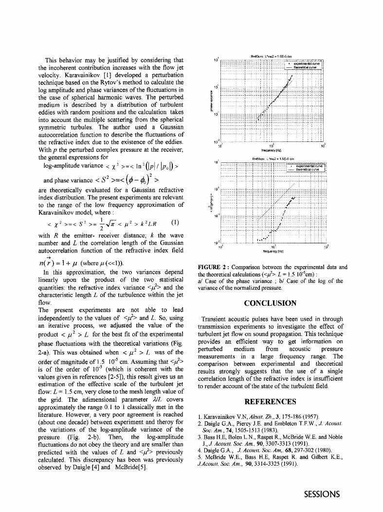
Statistics of the meteorological conditions favourable topropagation according to the three definitions

K. Rudno-Rudziński

Institute of Telecommunication and Acoustics, Wrocław University of Technology,Wybrzeże Wyspiańskiego 27, 50370 Wrocław, Poland, krr@zakus.ita.pwr.wroc.pl

Frequencies of the meteorological condition favourable to propagation according to the definitions of CONCAWE, ISO andNMPB were compared. Territories in Poland in different climate zones were chosen, in day and night time. Polar graphs of theconditions favourable to propagation show a lot of variability caused by the differences in the definitions. Variability causedby these differences is stronger than the one coming from the climate and the direction of propagation influences.

INTRODUCTION

The three classifications of meteorological condi-tions are likely the most popular in environmentalacoustics: CONCAWE [1], ISO [2] and IMPB [3]. Theaim of this work was to compare the statistics of theconditions favourable to propagation (CFTP) accord-ing to above mentioned definitions.

DEFINITIONS

In the ISO definition the wind velocity and directiondecides that the conditions are favourable. In the re-maining two the atmospheric stability is the secondmain factor besides of the wind. In CONCAWE thePasquill classification and the wind velocity compo-nent in the direction of propagation are used, in theNMPB some practical stability classes are employedtogether with the wind velocity and direction. In spiteof some similarity in wind and stability classes, thereare differences between CONCAWE and NMPB injoining them in the outcoming classes of propagationconditions.

ANALYSED DATA

Meteorological observation from the three stationslying in different climatic region were chosen for thisresearch (Table 1)[4]. The data set contains the resultsof observation made in three-hour cycles during theone whole year. Only the observations with the windbelow 5 m/s were included (67 % in Łeba, 76 % inWarszawa and 85 % in Wrocław).

Table 1. Three meteorological stations

Localisation Main climate influences Wind rose typeŁeba seaside breezeWarszawa continental bipolarWrocław oceanic uniform

STATISTICS

The calculated frequencies (percent) of the CFTPversus the direction of propagation are shown on theradar graphs with the angular resolution of 30o. Frequencies for the day time and the night time areshown on the Figure 1 and Figure 2 for Wrocław sta-tion as an example. Graphs of CFTP for the ISO defi-nition correspond to the smoothed wind rose (180° re-versed). Frequencies according to CONCAWE arehigher than to ISO, for the day and the night. For alldefinitions, frequencies according to NMPB are lowestfor the day and highest for the night. Such a regularityoccurs in the all stations.

0

10

20

30

400

30

60

90

120

150

180

210

240

270

300

330

CONCAWE ISO NMPB

Wrocław day

FIGURE 1. Percent of CFTP for Wrocław in the day timeaccording to the three definitions.

010203040506070

0

30

60

90

120

150

180

210

240

270

300

330

CONCAWE ISO NMPB

Wrocław night

FIGURE 2. Percent of CFTP for Warsaw in the night timeaccording to the three definitions.

Figure 3 shows frequencies of the CFTP conditionsaccording to NMPB for three stations, for the day (in-side) and for the night (outside). Table 2 shows the difference between the maximum andthe minimum frequency and between the mean frequenciesfor night and day.

010203040506070

0

30

60

90

120

150

180

210

240

270

300

330

Łeba Warszawa Wrocław

day

night

NMPB

FIGURE 3. Percent of CFTP according to NMPB for thethree stations in the night time and the day time.

Table 2. Difference between maximum and minimum fre-quency and between the mean frequencies for night and day

station method max-min(day)

max-min(night)

mean (night)-mean (day)

CONC 20,1 24,8 -2,0ISO 12,7 25,2 0,0 Łeba

NMPB 10,7 15,8 41,2CONC 10,1 7,5 7,5

ISO 13,8 9,7 0,0WarszawaNMPB 11,3 10,0 39,8CONC 3,2 21,2 7,8

ISO 14,9 22,5 0,0 WrocławNMPB 12,8 13,0 34,4

The difference between mean frequency of the CFTPfor the night time and the day time equals to zero forISO definition, ranges from –2 to 7,8 % for CON-CAWE and from 34,4 to 41,2 % for NMPB. The difference between the maximum frequency andthe minimum frequency of the CFTP (for all thepropagation directions in a given location) ranges from3,2 to 24,8 %.

CONCLUSIONS

The difference between mean frequency of the CFTPfor the night time and the day time equals to zero forISO definition, ranges from –2 to 7,8 % for CON-CAWE and from 34,4 to 41,2 % for NMPB. In the case of ISO definition the obvious reason ofthe lack of the difference between day and night is theneglect of the atmospheric stability. The lack of the difference in frequency of the CFTPbetween night and day indicates the same outdoorsnoise attenuation what is inconsistent with the experi-ence. From this point of view, NMPB gives likely the bestclassification method for the meteorological conditionsof sound propagation outdoors. Additional calculations indicates that CONCAWEcould be corrected to better differentiate day and nightconditions, maintaining precision of wind velocityquantification resulting from wind vector.

REFERENCES

1. K. J. Marsch, Appl. Acoustics, 15, 411-428 (1982)2. Bruit des infrastructure routiere - methode de calcul

incluant… CERTU, CSTB, LCPC, SETRA (1997)3. ISO 1996, 96134. K. Rudno-Rudziński, Meteorological conditions of sound

propagation outdoors in Poland, in Proceedings of theSixth ICSV, Techn. Univ. of Denmark 1999, pp.749-756

Split Mufflers for Improved Aerodinamic forVentilation Systems

O.V.Plitsina, V.T.Plitsin, M.N.Kucherenko

Togliatti Polytechnical Institute, Belorusskaya 14, 445667 Togliatty, Russia

Split mufflers suggested by the authors provide equal wide-band noise reduction in air conduits of large cross-section,have stable characteristic in two-phase flows. Aeroacoustic test of split designs is presented. Their acceptability for ventilationsystems with aerodynamic limitations is shown. Effective noise reduction and aerodynamic resistance decrease may be achievedby the splits orientation in parallel to the larger side of design’s cross-section.

Split mufflers were suggested for noise control offans mounted in systems with large cross–section ducts(having characteristic dimensions which are larger thanthe wavelength of propagating sound). In order toobtain muffler characteristics the aeroacoustic stand formodel (1 : 10) experiments was used.

The stand is mounted in three separate roomswith 400 mm thickness brick walls (Fig. 1).

FIGURE 1. Scheme of aeroacoustic stand

High pressure fan 1 entering into the stand has direct–current motor. The motor is supplied from voltagecontrol source 23. It allows to change flow of air in theair conduit 4 from 0 to 1000 m³/h. Fan’s aerodynamicnoise is reduced in the tubular muffler 3 joined withthe fan by the flexible insertion 2. In order to measureflow of air the diaphragm 6 having manometer tubes 7and micromanometer 19 are used. In order to measurepressure of air passing through the diaphragm 6 the U–tube manometer 18 is joined to manometer tube 5.The air conduit 4 is joined with inlet of the reverberantchamber 8 in which the sound columns 11 and thecondenser microphone 10 on the support are mounted.The air conduit with the replacement sections 13 isjoined to outlet (in direction of stream) of thereverberant chamber 8. There are manometer tubes 12for the U–tube manometer 18 joining in thereplacement sections. The air conduit with the

replacement sections is ended with trumpet in inlet ofthe reverberant chamber 14. Air goes out the chamber14 to room through the nozzle 17. The condensermicrophone 16 is placed into the chamber 14 on thesupport. Set of the replacement sections 13 allows tomount various length split mufflers between thereverberant chambers 8 and 14. The reverberantchambers 8 and 14 are welded 4 mm thickness platesteel structures having ribs. All chambers’ surfaces arenot parallel. The chambers have the doors 9 and 15.The doors are fulfilled from steel corners sheathed by 4mm thickness plate steel with packing over theperimeter by sponge rubber. Each chamber is mountedon rubber shock dampers. Leads input is fulfilled inthe chambers (to the microphones 10, 16 and soundcolumns 11) through packing glands. The chambershave nozzles for insertion of starting pistol used inreverberant time defining. The instrumentation isplaced in the room situated between the rooms with thereverberant chambers. In acoustic testing the signal istransferred from the rose noise oscillator 21 to theamplifier 20 joint with the sound columns 11. Soundoscillations arising in the reverberant chamber 8 aresensed by microphone 10, sound oscillationstransmitted through the testing split muffler are sensedby microphone 16. The signal is transferred from themicrophones to the B&K complex of the measuringapparatus 22 for precise laboratory and nature testing.The complex allows to obtain noise characteristic infrequency bands of set width in the such form asdigital presentation, curve on the recorder or on thecathode – ray oscillograph.

Stand’s chambers was attested before mufflerstesting with taking into consideration requirements ofISO documents.

It was tested on the stand: the model of onesection muffler; the model of two sections muffler withthe same sections; the model of two sections mufflerhaving sections with opposite orientation splits.

The model of one section muffler has built–upsteel body of rectangular shape (Fig. 2).

The model of two sections muffler with thesame sections is successive arrangement of themufflers with horizontal splits. The replacement airconduit 273 mm long is placed between the mufflers.

The model of the muffler having sections with oppositeorientation splits includes the muffler with horizontalsplits, replacement air conduit 273 mm long and themuffler with ten vertical splits. Section’s vertical andhorizontal splits are identical.

According to acoustic characteristics splitmufflers provide even broad –band noise reduction.Minimum effectiveness of the one section muffler(design is not optimized) is 4 dB; minimumeffectiveness of the muffler having two sections withopposite orientation splits is 8 dB. The acousticcharacteristic of muffler including the same sectionscoincides with the characteristic of one section muffler.Experiments show that influence of air stream movingwith speed to 18 m/s through the models of muffler onacoustic characteristics is insignificant and it may bedisregarded.

In obtaining aerodynamic resistance in the modelsthe air speed was being changed from 3 to 18,5 m/sand the flow was being changed from 160 to 1000 m³/hcorrespondingly. Experimental data was twelvemeasurements averaged. Confidence interval wascalculated for probability 0,95 and instrumental error2,5 %.

According to experiment (Fig. 3) friction andlocal resistance pressure loss in the split muffler ∆P, Pais

∆P = k Q²,where k – characteristic of resistance, Pa/(m³/h)²;

Q – flow of air, m³/h.The number of splits influences k value significantly.Its decrease from 13 (muffler with horizontal splits) to

10 (muffler with vertical splits) results in k reductionfrom 1,87·10–3 to 1,2·10–3 Pa/(m³/h)² in one sectionmuffler. Correspondingly the aerodynamic resistancedecreases on 36%. In adding section the pressure lossincreases in 2 time in case of the same splitsorientation and in 1,6 times in case of opposite

orientation. Hence, in order to increase aerodynamicresistance the split muffler should be designed withrectangular shape cross–section breaked up in parallelits larger side. In estimating acceptability of pressure

loss it was took into consideration design difference ofsplit muffler (bars) and baffle–type silencer (baffleswith thickness about 200 mm). In increasing splitmuffler rectangular cross – section in 1,5 times andfulfilling suggested splits orientation pressure loss insplit mufflers and in baffle–type silencer are the same.Thus split mufflers may be used in systems withaerodynamic limitations.

FIGURE 2. Model of one section muffler with horizontal splits

FIGURE 3. Pressure loss-air flow relation: 1- mufflerwith horizontal splits; 2- muffler with vertical splits.

FIG. 2 FIG. 1

1

e

f

f

f

TLL

TL

4kR

rf−

−+=

FIG. 4

FIG. 3

Acoustic Analysis Aimed At Characterizing

Combustion Instability In Premixed Burners

M. Annunziatoa, G. Coppola, M. Presaghia, R. Presaghi, G. Puglisi, F. Romanello a

a ENEA Ingegneria ed Impianti di Generazione di Energia, 00060 Roma, Italia New method to determine combustion characteristics by means of acoustic noise generated by dimensional variations of the flame due to unstable operation of the burner. The method allows to test efficiency of a burner and to deeply understand the causes that originate some problems related to the combustion.

METHOD OF ANALYSIS A method to characterize burners used in energy

generation plants is presented. The method has demonstrated to be particularly useful to put into evidence the anomalies presented by premixed burners in some operation regimes. In premixed burners, fuel and air are premixed before their entering combustion chamber. Differently from other burners, the premixed ones operate at lower temperatures, thus emitting less quantity of pollutants, but, although having these positive characteristics, they are affected by unpredicatble operation criticities, that cause a lowering in efficiency, environmental pollution and dangerous structural stresses [1]. The method is based on the principle that the burner represents a true acoustic cavity, containing both “flame fluid” and “exhaust fluid”. The different mechanical impedances and the dimensions of such fluids, determine the resonance frequency of the cavity. Acoustic effects of the said cavity move the noise band and center it on the resonance value. Consequently, by monitoring the latter parameter, it is possible to detect its cause: the variation in flame’s activity. FIGS. 1 and 2 represent a schematic view of two dimensional aspects of the flame due to the up mentioned phenomenon. When dimensional variation in the flame occurs with no variation in the quantities of air and fuel entering the burner, a flame instability [2] is experienced. Such instabilities are due to a series of causes that are originated by the reciprocal interaction of many parameters; for instance, pressure fluctuations generated by acoustic noise, act on combustion chemistry and determine chaotic evolutions in the phenomenon. However, the principle

on which the method is based remains a valid one. The photographic series of FIG.3 (a-f) shows a

typical evolution of the flame in instability conditions. The most important information that are possible to gain from noise are the thermal power variation and the dimensional variation of the flame, being the former correlated to noise amplitude and the latter to its dominant frequency. With the aim of evidencing the effects induced by the flame on the cavity’s resonance

frequency, a simplified formula is reported, based on the principle [3] that the resonant acoustic wave propagates itself into a cavity in a time that equals ¼ of its period. The simplification concerns the disposition of the two fluids (flame and exhaust gas) that occupy volumes that are adjacent, not in communication, and having each constant temperature, Tf e Te (FIG. 4).

(1) fr= resonance frequency [Hz]; Lf=flame length[m]; L=cavity length [m]; k=adiabatic index; R= specific gas constant [J/kg K= m2/s2 K].

140 150 160 170 180 190 200

0 0.1 0.2 0.3 0.4 0.5 0.6 0.7 0.8 0.9 1 flame lenght [m]

Tf = 1400°C Te = 550°C L = 1m

FIG. 5

Freq

uenc

y (H

z)

Freq

uenc

y

Time (ms)

FIG. 6 min

Am

plit

ude

Max

FIG. 8

The trend of fr versus Lf is shown in FIG.5, assuming k and R to be the same for both fluids, that is not relevant for our aim. The instrumental analysis of the phenomenon has been thus conducted on the basis of the up mentioned considerations.

Processed signals are originated by two different types of sensors: acoustic-electric transducer (microphone) and pressure gauge connected to combustion chamber. Both the signals allowed to catch the combustion instability phenomenon, also considering that the microphone signal contained some noise coming from external environment.

FIG. 6 represents a three-dimension diagram (time,

frequency, amplitude) obtained by the wavelet transform technique. In this figure many frequency excursions are noticed, while only once it appears an event associated to high instability. This shows how not always an high variation in the thermal power of the flame is associated to a change in its dimensions.

Similar results have been obtained when processing the signal by means of a frequency discriminator. One example is reported in FIG.7: diagram a) reproduces combustion noise, while b) represents the frequency deviation of the noise itself. It

can be evidenced how b) has a trend similar to the envelopment of a) and presents noticeable variations also at times in which a) assumes reduced values. In this way, signal b) has the peculiarity to detect the flame’s instability ranges, this in advance to the statistical occurrence of strong instabilities. FIG. 8 shows the front panel of the final software device (realized by LabView), based on the up mentioned discriminator. The instrument in the upper right corner of the figure shows a bar graph generated by five different operation conditions of the burner,

respectively having the following values of λλ: 1.1; 1.2; 1.3; 1.4; 1.5 ( λλ meaning the ratio between introduced air quantity and steichiometric one). Values of λλ of 1.1 and 1.5 are the operation limits of the investigated burner. The highest bar is referred to the most unstable condition of the flame; the third condition appears to be the most stable one, then the bars start to increase again their height. The bars represent the energy of the signals shown in FIG. 7, b), that have been previously filtered as to eliminate the components that are not correlated to the phenomenon. Asymmetry in hystogram is due to the different instability types (mixtures close to the steichiometric value and mixtures with air eccess). Every other device of the front panel is used to set the parameters of the analysis or to control their different phases.

CONCLUSIONS

This study has been carried out to detect a methodology able to give more information when compared to the already known ones; this has been obtained considering the burner to act as a resonant cavity and thus generating the idea to detect the induced effects on the combustion generated acoustic noise: that is the variation in dominant frequency of the noise itself. On the basis of the obtained results, the method appears to be suitable for carrying out analysis aimed at the knowledge of burner efficiency and the one of its control system.

REFERENCES

1. Lefebrve A. H., Gas Turbine Combustion, Mc Grow-Hill, New York, 1983.

2. McManus K. R., Poinsot T. and Candel S. M., A Review of Active Control of Combustion Instabilities, Progr. Energy Combustion Science, 1993, vol 19, pp 1-29.

3. Javorskij B.M., Detlaf A. A., Spravoènik po fisike, Mir pubblisher, 1977

Time FIG. 7

Max

min

Freq

uenc

y A

mpl

itude

Higher mode cylindrical radiatorfor an aerial intense ultrasound source

H. Yamanea and T. Otsukab

aDepartment of Electrical Engineering, College of Science and Technology, Nihon University1-8 Surugadai, Chiyoda-ku Tokyo 101-8308, JAPAN

bDepartment of Electrical and Electronic Engineering, College of Industrial Technology,Nihon University 1-2-1 Izumicyo, Narashino, Chiba 275-8575, JAPAN

This work deals with a development of a cylindrical radiator for industrial applications such as collecting fine oil mist

that floats in air. The thickness of the cylindrical radiator was selected so as to be within the range of the flexural

vibration. The radiator was driven by a Bolt-Clamped Langivin transducer(BLT). The stripe mode vibration was

obtained on the radiator while the flexural vibration appeared along the radiator axis. The resonance frequency of

the cylinder itself and the ultrasound of a radiator in the cylinder were adjusted at the same frequency to produce a

high intensity ultrasound field. As a result, the sound pressure level in the cylinder up to 170 dB was obtained. This

makes it possible to use the system in the industrial application of collecting and/or coagulating fine oil mist floating

in air.

CYLINDRICAL RADIATOR

The frequency of the (m,s) mode in the cylindri-cal radiator1) is given by

fms = αmsc

2πr(1)

where m, s − 1 are the number of nodal diam-eters and the number of nodal circles, αms is theeigenvalue given by m

αmsJm(αms)−Jm+1(αms) = 0,

where Jm, Jm+1 are cylindrical Bessel functions ofthe m-th and (m + 1)-th order and c is the velocityof sound, r is the radius of cylinder.

The m-th order of the resonance frequency ofthe flexural vibration on the cylinder surface 2) isdetermined for the number of m mode lines as

fm =NmCMh

2π(r + h/2)2(2)

where Nm = m(m2−1)√m2+1

, CM is the material con-

stant and determined from(=

√E

12ρ(1−ν2)

), where

E is the Young’s module of elasticity, ρ is the den-sity, ν is the Poisson’s ratio and h is the cylinderthickness.

The cylinder radius at the (m,s) mode is ob-tained using Eq. (1)

r = αmsc

2 π fms(3)

The thickness h is determined by the followingmethodology:Substitute fms for fm from Eq. (2) into Eq. (3) andthe resulting thickness h is obtained by the followingexpression

h = −2(r − NmCM

2πfms

)+

√(r − NmCM

2πfms

)2

− r2 (4)

SOUND PRESSURE DISTRIBUTION IN-SIDE THE CYLINDER

The Root-Mean-Square value of the sound pres-sure level distribution inside the cylinder is given by

P = Jm(αms r) · cos mθ (5)

Table 1 gives the dimension of the cylindricalradiator calculated from Eqs. (3) and (4).

Table 1. Details of cylindrical radiator(m,s) Inside radius Thickness Length Frequency

r [cm] h[cm] l [cm] f[kHz]

(11,5) 7.715 0.48 9.30 20.90

Figure 1 shows the sound pressure level distri-bution inside the cylinder as calculated by equation(5). There are 11 nodal diameters and four nodalcircles.

Figure 1. Sound pressure level distribution insidethe radiator at the frequency of 20.9 kHz byEq.(5).

DRIVING UNIT

The schematic of the driving unit is shown inFigure 2. The BLT at the frequency of 20 kHz isconnected to a half wavelength exponential horn,the cylindrical radiator is driven by the horn.

nodal lines

Figure 2. Cylindrical radiator for the frequency of20.9 kHz. The stripe mode can be observed on theinner surface of the radiator.

ACOUSTIC CHARACTERISTICS

The sound pressure level distribution was mea-sured along the radius with the maximum soundpressure levels occurring on the central axis insidethe cylinder.

0 2 4 6 80

0.5

1

Distance from center axis of cylindricalradiator [cm]

Nor

mal

ized

sou

nd p

ress

ure A

Figure 3. Normalized sound pressure distribution.

The sound pressure level was measured with a1/4 ” condenser microphone with the probe tubewhen the electric power of 20 W was applied to theBLT. The probe tube is 20 cm long, has 0.15 cminner diameter and is 0.05 cm thick. The measuredsound pressure level distribution is in good agree-ment with the calculations.

Fig. 4 shows the linearity of the acoustic poweras measured with a 1/8 ” 4138 microphone. Themicrophone was located at the point A in Figure3. The sound pressure is proportional to one halfthe input electric power and 5.64 kPa (169 dB) wasobtained at 200 W of input power.

10 1001000

2000

3000

4000

5000

6000

7000

160

170

Electric input power [W]

Sou

nd p

ress

ure

[Pa]

Sou

nd p

ress

ure

leve

l [d

B]

Figure 4. Linear characteristic of the soundpressure versus the input electric power.

CONCLUSIONS

The cylindrical radiator with radial flexural vi-bration was designed to operate at the frequency of20.9 kHz. The radiator is made of titanium and thesound pressure levels of 169 dB were obtained at200 W of electric power input.

This system can be used in industrial applica-tions as a tool that would enable attraction andcoagulation of the fine free-floating oil mist.

REFERENCES

1) McLanchlan, N. W., Bessel function for engineer-ing. Oxford University Press, London 1955.2) Timoshenko, S. P., Young, D. H.,& Weaver, W.Jr., Vibration Problems in Engineering. John Wiley& Sons, New York 1974.

Figure 1. Geometry of the system

A propagation of acousto-gravity waves inatmosphere has been studied rather intensively[1-3]. These waves are considered often as oneof basic channels of energy exchange betweenlithosphere and ionosphere caused by differentdisturbances of both seismic and space nature(see, for example, [4-6] and references therein).The main consequence is the exponential growthof amplitude of the oscillatory velocity ofparticles with an altitude. Certainly, such agrowth is limited by the account of such factorsas viscosity of air, and also of convectivenonlinearity in equations of motion. As it isshown below, the very important factor is alsomutual coupling of acousto-gravity waves withanother excitations in the ground, one of them isthe Rayleigh wave in the Earth crust.Generally, an influence of the sound in air on apropagation of Rayleigh waves in a substrate isvery little, because of a great difference of thedensities of environments. However, such aninfluence, as it was marked in [6], becomesessential in the point of intersection ofdispersion branches of the Rayleigh wave in asubstrate with the volume branch of the soundwave in the air when the phase velocities ofwaves become equal. Such a point refers to as acoupling point, or a point of synchronism. In avicinity of such a point, the mutual influence ofwaves becomes strong. Particularly, thisconcerns to a case when the gravity force isessential and the acoustic waves in atmospherebecome of acousto-gravity type. It is impossibleto investigate the wave subsystems in air andground separately in a vicinity of a synchronismpoint. In this case, the aero - hydrodynamic

system in atmosphere and the system of theoryof elasticity in ground should be solved jointly.The propagation in an atmosphere of theseismically excited sound waves causesoscillations of the ionosphere - atmosphereboundary. As a result, Doppler reflections ofelectromagnetic waves from ionosphere layers atfrequencies 10 and 25 MHz were observed [7].

Those observations demonstrated that theRayleigh waves can propagate to considerabledistances from a source (about 5000km). As thiseffect was detected rather far from a seismicsource, it is apparent that in such conditions theRayleigh wave propagated as an own wave of alayered system. During such propagation, theconditions of a synchronism with waves inatmosphere can be reached. Therefore,understanding the features of interaction of aRayleigh wave with acousto-gravity waves invicinity of a point of a synchronism is importantto see over the total physical picture. However,in this case the problem becomes more complex,as it is necessary to take into account for bothwaves under equal conditions. We should solvethe coupled acousto-gravity - sound problem bya self-consistent way.

Variations of transverse structure of coupledacousto-gravity - Rayleigh waves in multilayered

system Earth - atmosphere

G. Burlak, V.Grimalsky, S. Koshevaya

Center for Research on Engineering and Applied Sciences, Autonomous State University ofMorelos,Z.P. 62210, Cuernavaca, Mor., Mexico.E-mail: gburlak@uaem.mx

The transverse distribution of coupled acousto-gravity waves in atmosphere and a Rayleigh wave in a layeredsystem Earth - atmosphere is investigated. The special attention is given to a mode of strong coupling ofwaves in a solid substrate with the oscillations in upper medium (atmosphere) when the phase velocities ofwaves are close (coupling point, or a point of synchronism). Is shown that in this point the frequency shiftinduced by the mutual influence of waves becomes maximal. In vicinity a coupling point, a strong change ofthe cross structure of wave in air takes place.

0 1 2 3 40

0.2

0.4

0.6

0.8

1

1.2

1.4(a)

kh

Re(

x)

0 1 2 30

0.02

0.04

0.06

0.08

0.1(b)

kh

Im(x

)

0 1 2 3 40.1

0.15

0.2

0.25

0.3

0.35(c)

kh

v, k

m/s

ec

vgr

→

vph

↑

0 1 2 3 4−0.2

−0.1

0

0.1

0.2

0.3

0.4

0.5(c)

kh

Re(

κ +)

Figure 2. Dependencies of real and imagineparts of a wave frequency (a,b), phase and groupvelocities (c), and the transverse wave numberκ+of the acoustic-gravity wave in the air (d)

In this report, the transverse distribution ofcoupled acousto-gravity wave with a Rayleighwave in a layered system Earth - atmosphere isinvestigated. The motion equations has form[8]:

,)( zgpvvtv ∇+−∇=∇+

∂∂ ρϖϖϖ

k

iki

xp

tu

∂∂=

∂∂

2

2

γ (1)

The special attention is given to a mode ofstrong coupling of waves in a solid substratewith a sound in upper medium (atmosphere)when the phase velocities of waves are close(coupling point, or a point of synchronism). Weuse the dimensionless parameters x=ωh/ct1 andy=kh. In these variables, the dispersion equationhas a general form

),()2(),()/( 22

1

0222 yxFxyxDcxy n ηκγρ

+=− + (2)

Thus, the dispersion equation of sound waves inexamined system can be presented as

)2)(,(),( 22

0 ηκδκ += +yxFxyxD (3)where δ=ρ0/γ, κ0=y2-x2/c0n

2, c0n=c0/c1t. For acontact soil - air, it occurs δ=10-3<<1. At δ=0,equation (3) splits into two independentbranches: a volume wave in the air and a normalmode in a layered ground. We are interested inthe modes, which can intersect with a volumewave in the air. Note that second the lowestbranch of acousto-gravity wave [4] does nothave intersection with the Rayleigh wave. Thisbranch is not studied here. At δ≠0, the wavesbecome coupled. However, as δ<<1, thiscoupling is weak and it results in the smallfrequency shift. We found that in this point thefrequency shift induced by the mutual influencewaves becomes maximal. In vicinity a couplingpoint, a strong change of a cross structure ofwave in air arises. The strong dependence of afactor of the exponential growth of an oscillatoryvelocity of acousto-gravity waves with analtitude due to parameters of a solid substrate isdemonstrated. It is shown that the frequencyband of the exponential growth is limited onhigh frequencies. As a result, a wave becomeslocalized near the surface of the Earth at higherfrequencies. The point of the change fromincrease to decreasing is determined by a pointof a synchronism with a Rayleigh wave in theground substrate. Fig.2 presents thedependencies of real and imagine parts of awave frequency (a,b), phase and group velocities(c), and the real part of coefficient κ+ of thewave in the air(d) of a coupled wave in the

system Earth - air versus the value of y=kh forpointed above parameters. These dependenciesare obtained by a direct numerical solution of thedispersion equation. It is seen from the Fig.2 (b)that in the left side from coupling point theattenuation of waves is unessential but itincreases sharply in the right hand side from thispoint yh=2.6. This increase is due to a moredeep penetration of the wave into the soil wherea viscosity is not equal to zero. Also one can seefrom the Fig.2(d) that in the left side from thepoint of coupling the most part of the wave isdelocalized (Re κ+<0 on z<0; in the right sidefrom this point the wave is concentrated mainlyin the solid substrate z>0. The account ofviscosity in soil causes weak wave attenuationbut does not change a general physical picture ofthe wave interaction.

ACKNOWLEDGEMENTThis work is supported by CONACYT project#35455-A.

REFERENCES1. Hocke, K. and Schlegel, K., Ann. Geophys.12, 917 (1996).2. Hunsucker, R.D., Rev. of Geophys. and SpacePhys. 20, 293 (1982).4. Gossard, E. E. and Hooke, W. H., ''Waves inthe Atmosphere'' (Elsevier, Oxford, 1975).5. lngersoli, A.P., Kanamori, H. and Dowling,T.E., Geophys. Res. Lett. 21, 1083 (1994).6. Ewing, W.M., W.S.Jardetsky, W.S. and Press,E., ''Elastic Waves in Layered Media'' (McGraw-Hill, New York, 1957).7. Weaver, P.F., P.C.Yuen, P.C., G.W.Prolls,G.W. et al., Nature, 226, 1239 (1970).8. Brekhovskikh, L.M., ''Waves in LayeredMedia'' (Pergamon Press, Oxford, 1985).

Measurements of Aerodynamic Velocity Fields With AnAcoustical Probe

V. Dewailly, F. Cohen Tenoudji, J.P. Frangi and M. de Billy

Laboratoire Environnement et Développement, Université D. Diderot, Tour 33-43, Case postale 7087,2 place Jussieu, 75251 Paris Cedex 05, France.

e-mail : dewailly@ccr.jussieu.fr

A system using the displacement of a three-axis ultrasonic anemometer probe in the air flow within a wind tunnel is used to probethe local variations of the flow velocity. The three velocity components are calculated from the sound travel times betweentransducer pairs placed in opposition (three pairs ; 44 kHz frequency). For each probe location, 400 velocity vector data values aremeasured at 32Hz. The average velocities and their fluctuations along the main axis of the flow and in the transverse plane arepictured as images coded as false colors or vector arrows. The spatial resolution of the 22 cm x 22 cm images is in the order of 1cm after correction of the bias brought by a particular probe orientation. The technique shows good reproducibility in the air flowcharacterization. Acoustical results are compared with those obtained by an optical technique for different air flow situations.

The sound scattering by a moving fluid is an importantproblem which has received a considerable experimental andtheoretical interest since many years [1-3]. The interaction ofacoustic waves with a turbulent flow is used to visualize thevelocity field near a square outlet at moderate Reynoldsnumber. This experimental method is not intrusive and doesnot necessitate additional matter. The average field velocityfluctuations - which are generated by the turbulence - areplotted in a plane perpendicular to the flow axis and in thedirection of the air flow. The patterns obtained with andwithout a grid (located at the outlet) are compared andanalyzed.

EXPERIMENTAL SET-UP

A sonic thermometer – anemometer (type CSAT 3 fromCampbell-Society) is used for the measurements. It includesthree non – coplanar pairs of ultrasonic transducers operatingabout 40kHz and is attached to an X-Y linear displacementequipment which lets the transmitters to move accurately bystep of 10mm which determines the spatial resolution. All thedisplacements are driven by a computer. The jet flow isproduced by a rotating fan placed in the central sectionsituated between the square (22x22cm2) inlet and outlet.

XY

Z

G r i dF a nA i r f l o w

The components of the velocity vector are recordedsimultaneously in three orthogonal directions. The z-component (or axial velocity) coincides with the axis of thepropeller (see Fig.1). Because of the fluctuation of thevelocity of propagation of the sound in the turbulent medium,the arrival time varies and for each probe location 400velocity vector data values are measured at 32Hz. Theturbulence is supposed to be stationary. The measurementsare achieved in a (X,Y) plane located at 4cm from the outlet.

RESULTS AND ANALYSIS

In figure 2-a are plotted the diagrams of the velocity fields(represented by vector arrows) obtained in the X-Y plane andwithout any grid (vertical and horizontal scales are in cm).

0 5 1 0 1 5 2 0 2 50

2

4

6

8

1 0

1 2

1 4

1 6

1 8

2 0

On the picture we observe only one vortex the origin ofwhich is the rotation of the fan. No such behavior is noticedin the figure 3-a which represents the velocity field diagramwhen a grid is introduced between the outlet and theanemometer. The dimensions of the grid are 1x1x1cm3. Noperiodicity characteristic of the grid may be extracted from

FIGURE 1 : Schematic diagram of the experimentalset-up.

FIGURE 2-a : Velocity field in the X-Y plane(without grid).

this plot. In figures 2-b and 3-b are showna gray-scaledistribution of the z-component velocity measured with andwithout the grid respectively. In the center of the first picture,

0 2 4 6 8 1 0 1 2 1 40

2

4

6

8

1 0

1 2

1 4

1 6

1 8

we may the presence of negative values of the axial velocitywhich result from the conjugated effects: the existence ofhigh velocity components near the periphery and the presence

of a virtual “tube” in which the z-component velocity value iszero.

The second figure confirms that there is no more negativecomponent of the velocity.

CONCLUSION

The measurements previously described and limited to thecomparison of results obtained with and without grid may beextended to the velocity fields measurements behindaxisymmetric targets. Temporal inter-correlation and auto-correlation should be calculated to get additionalcharacteristics of the fields velocity and to gather moreinformations on the energy exchange between the differentcomponents of the velocity.

REFERENCES

1. Petrossian, A., and Pinton, J.F., J. Phys. II France 7, 801-812 (1997).2. Baudet, C., Ciliberto, S. and Pinton, J.F., Phys. Rew. Lett.,67, 193-195 (1991).3. Wen-Shyang Chiu, Lauchle, G.C. and Thompson, D.E., J.Acoust. Soc. Am., 85, 641-647 (1989).

FIGURE 2-b : Gray representation of theaxial velocity (without grid).

FIGURE 3-a : : Velocity field in the X-Yplane (with grid).

FIGURE 3-b : Gray representation of theaxial velocity (with grid).