Embed Size (px)
Citation preview
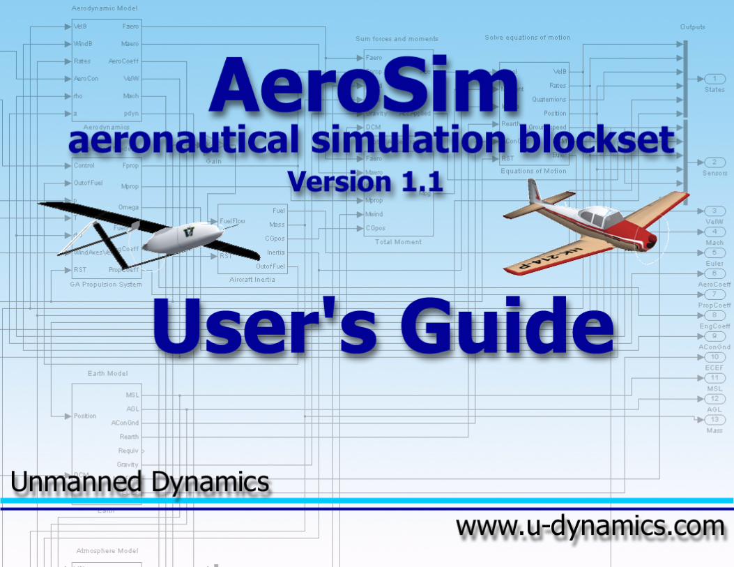
AEROSIM BLOCKSETVersion 1.1
User’s Guide
Unmanned Dynamics, LLCNo.8 Fourth St.
Hood River, OR 97031(541) 308-0894
http://[email protected]
Contents
1 Introduction 11.1 Software Changes from Version 1.01 to 1.1. . . . 11.2 Software Changes from Version 1.0 to 1.01. . . . 11.3 New Features for Version 1.01. . . . . . . . . . . 21.4 Keeping up-to-date with the AeroSim Blockset:
The AeroSim Mailing List . . . . . . . . . . . . . 21.5 System Requirements. . . . . . . . . . . . . . . . 21.6 Contents of the installation CD. . . . . . . . . . . 31.7 Install the AeroSim Blockset. . . . . . . . . . . . 31.8 Uninstall the AeroSim Blockset. . . . . . . . . . 4
1.9 Library Description. . . . . . . . . . . . . . . . . 4
2 Aircraft Model Demos 62.1 Open-loop Flight . . . . . . . . . . . . . . . . . . 72.2 Lateral Control . . . . . . . . . . . . . . . . . . . 82.3 Airspeed Control . . . . . . . . . . . . . . . . . . 92.4 Wind Effects . . . . . . . . . . . . . . . . . . . . 122.5 Inertial Navigation . . . . . . . . . . . . . . . . . 142.6 Joystick Control. . . . . . . . . . . . . . . . . . . 152.7 Interfacing to FlightGear Flight Simulator. . . . . 162.8 Interfacing to Microsoft Flight Simulator. . . . . . 182.9 FlightGear Aircraft Demos. . . . . . . . . . . . . 20
AeroSim Blockset User’s Guide CONTENTS
2.10 Aircraft Model Trim and Linearization. . . . . . . 21
3 Setting-up and Running an Aircraft Model 263.1 Aircraft Model Examples. . . . . . . . . . . . . . 273.2 Building an aircraft configuration. . . . . . . . . . 28
3.2.1 Conventions . . . . . . . . . . . . . . . . 283.2.2 Section 1: Aerodynamics. . . . . . . . . . 283.2.3 Section 2: Propeller. . . . . . . . . . . . 293.2.4 Section 3: Engine. . . . . . . . . . . . . . 303.2.5 Section 4: Inertia. . . . . . . . . . . . . . 313.2.6 Section 5: Other parameters. . . . . . . . 31
3.3 The pre-built Aircraft Models. . . . . . . . . . . . 323.4 Using FlightGear Aircraft Configuration Files. . . 35
3.4.1 The JSBSim XML Configuration File. . . 353.4.2 The xmlAircraft Parser. . . . . . . . . . . 363.4.3 The Matlab Aircraft Structure. . . . . . . 37
3.5 Additional Matlab Utilities . . . . . . . . . . . . . 40
4 Block Reference 414.1 Actuators . . . . . . . . . . . . . . . . . . . . . . 42
4.1.1 Simple Actuator (1st-order dynamics). . . 434.1.2 Simple Actuator (2nd-order dynamics). . 454.1.3 D/A Converter . . . . . . . . . . . . . . . 46
4.2 Aerodynamics. . . . . . . . . . . . . . . . . . . . 474.2.1 Aerodynamic Force. . . . . . . . . . . . . 484.2.2 Aerodynamic Moment. . . . . . . . . . . 494.2.3 Wind-axes Velocities. . . . . . . . . . . . 504.2.4 Dynamic Pressure. . . . . . . . . . . . . 524.2.5 Lift Coefficient . . . . . . . . . . . . . . . 534.2.6 Drag Coefficient . . . . . . . . . . . . . . 55
4.2.7 Side Force coefficient. . . . . . . . . . . . 574.2.8 Pitch Moment Coefficient. . . . . . . . . 584.2.9 Roll Moment Coefficient. . . . . . . . . . 604.2.10 Yaw Moment Coefficient. . . . . . . . . . 61
4.3 Atmosphere. . . . . . . . . . . . . . . . . . . . . 624.3.1 Standard Atmosphere. . . . . . . . . . . . 634.3.2 Background Wind . . . . . . . . . . . . . 644.3.3 Turbulence. . . . . . . . . . . . . . . . . 654.3.4 Wind Shear. . . . . . . . . . . . . . . . . 66
4.4 Complete Aircraft. . . . . . . . . . . . . . . . . . 674.4.1 6-DOF Aircraft Model - body-frame EOM 684.4.2 6-DOF Aircraft Model - geodetic-frame EOM714.4.3 6-DOF Aircraft Model - geodetic-frame EOM,
no magnetic field. . . . . . . . . . . . . . 744.4.4 Simple Aircraft Model. . . . . . . . . . . 774.4.5 Glider Model . . . . . . . . . . . . . . . . 794.4.6 Inertial Navigation System. . . . . . . . . 81
4.5 Earth. . . . . . . . . . . . . . . . . . . . . . . . . 824.5.1 WGS-84 . . . . . . . . . . . . . . . . . . 834.5.2 EGM-96 . . . . . . . . . . . . . . . . . . 844.5.3 Ground Detection. . . . . . . . . . . . . . 854.5.4 WMM-2000 . . . . . . . . . . . . . . . . 86
4.6 Equations of Motion . . . . . . . . . . . . . . . . 874.6.1 Total Acceleration . . . . . . . . . . . . . 884.6.2 Total Moment. . . . . . . . . . . . . . . . 894.6.3 Body-frame EOM: Forces. . . . . . . . . 904.6.4 Body-frame EOM: Moments. . . . . . . . 914.6.5 Body-frame EOM: Kinematics (Quaternions)924.6.6 Body-frame EOM: Kinematics (Euler An-
gles). . . . . . . . . . . . . . . . . . . . . 93
2
CONTENTS AeroSim Blockset User’s Guide
4.6.7 Body-frame EOM: Navigation. . . . . . . 944.6.8 Geodetic-frame EOM: Position. . . . . . 964.6.9 Geodetic-frame EOM: Velocity. . . . . . 984.6.10 Geodetic-frame EOM: Attitude (Quaternions)1004.6.11 Geodetic-frame EOM: Attitude (Euler An-
gles). . . . . . . . . . . . . . . . . . . . .1014.6.12 Geodetic-frame EOM: Angular Rate. . . . 102
4.7 Inertia . . . . . . . . . . . . . . . . . . . . . . . .1044.7.1 Aircraft Inertia . . . . . . . . . . . . . . .1054.7.2 Inertia Coefficients. . . . . . . . . . . . .107
4.8 Math. . . . . . . . . . . . . . . . . . . . . . . . .1084.8.1 Cross Product. . . . . . . . . . . . . . . .1094.8.2 Normalization . . . . . . . . . . . . . . .1104.8.3 Vector Norm . . . . . . . . . . . . . . . .1114.8.4 Non-zero Sign . . . . . . . . . . . . . . .1124.8.5 Zero Offset. . . . . . . . . . . . . . . . .1134.8.6 pi Bound . . . . . . . . . . . . . . . . . .1144.8.7 2pi Bound. . . . . . . . . . . . . . . . . .115
4.9 Pilot Interface. . . . . . . . . . . . . . . . . . . .1164.9.1 FS Interface. . . . . . . . . . . . . . . . .1174.9.2 FlightGear Interface. . . . . . . . . . . .1194.9.3 Joystick Interface. . . . . . . . . . . . . .1214.9.4 CH F-16 Combat Stick. . . . . . . . . . .122
4.10 Propulsion. . . . . . . . . . . . . . . . . . . . . .1244.10.1 Fixed-Pitch Propeller. . . . . . . . . . . .1254.10.2 Piston Engine. . . . . . . . . . . . . . . .1264.10.3 GA Propulsion System. . . . . . . . . . .128
4.11 Sensors. . . . . . . . . . . . . . . . . . . . . . .1304.11.1 Noise Correlation: Random Walk. . . . . 1314.11.2 Noise Correlation: Gauss-Markov Process. 132
4.11.3 Simple Sensor - 1st-order dynamics. . . . 1334.11.4 Simple Sensor - 2nd-order dynamics. . . . 1344.11.5 Analog Sensor. . . . . . . . . . . . . . .1354.11.6 A/D Converter . . . . . . . . . . . . . . .1364.11.7 Single GPS Measurement. . . . . . . . .1374.11.8 GPS PV. . . . . . . . . . . . . . . . . . .138
4.12 Transformations. . . . . . . . . . . . . . . . . . .1394.12.1 Body-Inertial DCM From Quaternions. . . 1404.12.2 Body-Inertial DCM From Euler Angles. . 1414.12.3 Body-Wind DCM. . . . . . . . . . . . . .1424.12.4 Euler Angles From Quaternions. . . . . . 1434.12.5 Euler Angles from DCM. . . . . . . . . .1444.12.6 Quaternions From Euler Angles. . . . . . 1454.12.7 ECEF Position. . . . . . . . . . . . . . .146
4.13 Unit Conversion. . . . . . . . . . . . . . . . . . .1474.13.1 Angular position: Deg 2 rad and Rad 2 deg1484.13.2 Angular velocity: Rad/s 2 RPM and RPM
2 rad/s. . . . . . . . . . . . . . . . . . . .1494.13.3 Distance: ft 2 m and m 2 ft. . . . . . . . .1504.13.4 Distance: m 2 nm and nm to m. . . . . . . 1514.13.5 Velocity: m/s 2 km/h and km/h 2 m/s. . . 1524.13.6 Velocity: m/s 2 mph and mph 2 m/s. . . . 1534.13.7 Velocity: m/s 2 kts and kts 2 m/s. . . . . . 1544.13.8 Force: lbf 2 N and N 2 lbf. . . . . . . . .1554.13.9 Mass: lb 2 kg and kg 2 lb. . . . . . . . . .1564.13.10 Mass: slug 2 kg and kg 2 slug. . . . . . . 1574.13.11 Volume: gal 2 l and l 2 gal. . . . . . . . .1584.13.12 Pressure: Pa 2 in.Hg. and in.Hg. 2 Pa. . . 1594.13.13 Temperature: K 2 F and F 2 K. . . . . . . 160
4.14 FlightGear-Compatible. . . . . . . . . . . . . . .161
3
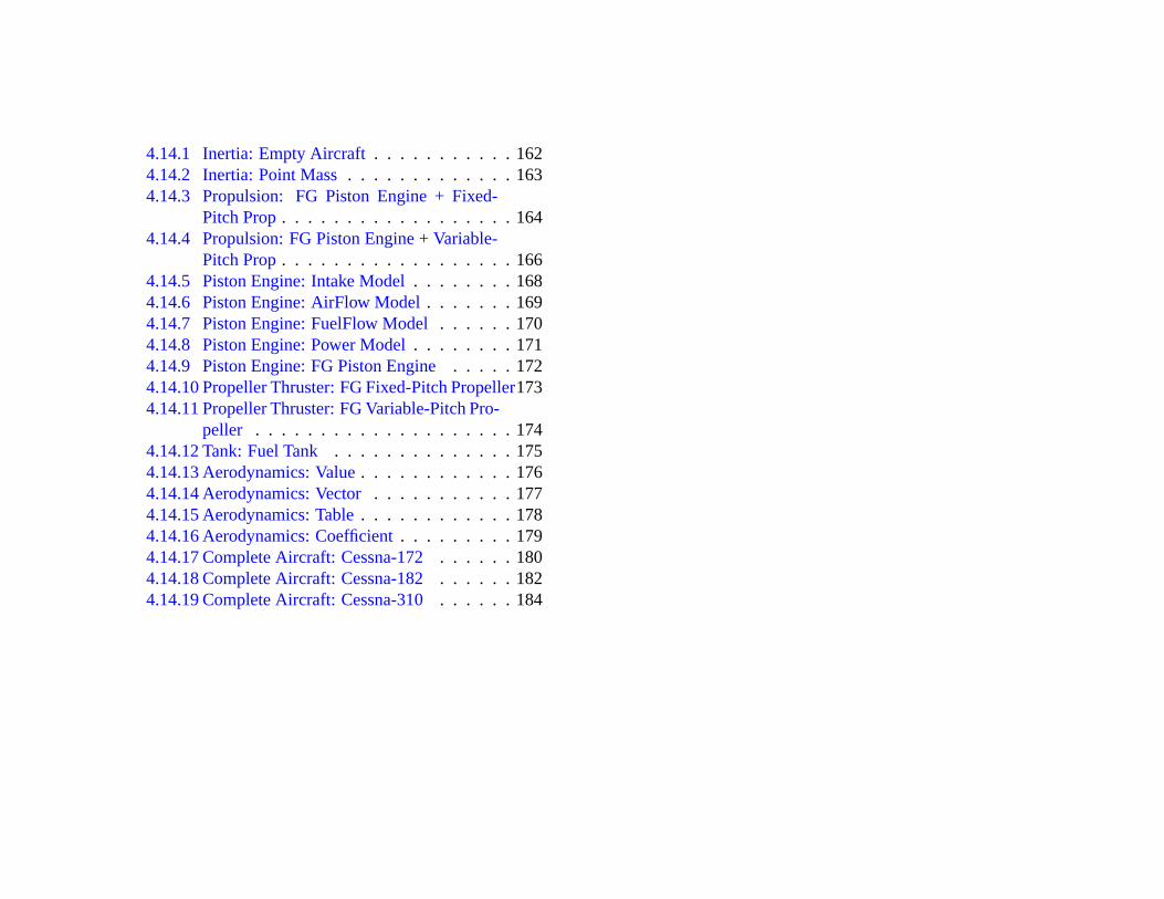
4.14.1 Inertia: Empty Aircraft. . . . . . . . . . .1624.14.2 Inertia: Point Mass. . . . . . . . . . . . .1634.14.3 Propulsion: FG Piston Engine + Fixed-
Pitch Prop. . . . . . . . . . . . . . . . . .1644.14.4 Propulsion: FG Piston Engine + Variable-
Pitch Prop. . . . . . . . . . . . . . . . . .1664.14.5 Piston Engine: Intake Model. . . . . . . . 1684.14.6 Piston Engine: AirFlow Model. . . . . . . 1694.14.7 Piston Engine: FuelFlow Model. . . . . . 1704.14.8 Piston Engine: Power Model. . . . . . . . 1714.14.9 Piston Engine: FG Piston Engine. . . . . 1724.14.10 Propeller Thruster: FG Fixed-Pitch Propeller1734.14.11 Propeller Thruster: FG Variable-Pitch Pro-
peller . . . . . . . . . . . . . . . . . . . .1744.14.12 Tank: Fuel Tank. . . . . . . . . . . . . .1754.14.13 Aerodynamics: Value. . . . . . . . . . . .1764.14.14 Aerodynamics: Vector. . . . . . . . . . .1774.14.15 Aerodynamics: Table. . . . . . . . . . . .1784.14.16 Aerodynamics: Coefficient. . . . . . . . .1794.14.17 Complete Aircraft: Cessna-172. . . . . . 1804.14.18 Complete Aircraft: Cessna-182. . . . . . 1824.14.19 Complete Aircraft: Cessna-310. . . . . . 184
1 INTRODUCTION AeroSim Blockset User’s Guide
1 Introduction
The AeroSim aeronautical simulation blockset provides a com-plete set of tools for the rapid development of nonlinear 6-degree-of-freedom aircraft dynamic models. In addition to the basic air-craft dynamics blocks, the library also includes complete aircraftmodels which can be customized through parameter files.
Since theAeroSim blockset components are built using onlybasic Simulink blocks and portable C/C++ code, you can useReal-Time Workshop to automatically generate source code fromyour aircraft models.
Aircraft model examples include the Aerosonde UAV and theNavion general-aviation airplane.
The library allows importation of XML FlightGear aircraft con-figuration files (JSBSim format). Sample blocks for the Cessna172, 182, and 310 based on JSBSim models can be found in theFlightGear-Compatible section of theAeroSim library.
1.1 Software Changes from Version 1.01 to 1.1
The following changes were done to existing library features:
• The FlightGear Interface now uses the latest version ofFlightGear which is 0.9.2. The interface S-function was up-dated to be able to connect to this version. TheC-172, C-182andC-310aircraft models were updated to make use ofthe latest version of the JSBSim aircraft configuration files.
• TheWind Force andWind Moment blocks were removedfrom the library; the wind effects are accounted for through
the aerodynamic model. The only outputs from the windmodel now are the wind linear and angular velocities.
• The Total Acceleration andTotal Moment blocks do nottake wind force and moment inputs anymore, since the windeffects have changed, as described in the item above.
• A bug in theInertia Coefficientsblock resulted in the wrongvalue being computed for the inertia coefficientc8. It is nowcorrected.
• The Simple Aircraft andGlider models were not runningdue to several variables being undefined. The models nowrun properly.
• A bug in theECEF Position block caused incorrect trans-formation from geographic coordinates to Earth-centered Earth-fixed frame. The bug has been fixed.
1.2 Software Changes from Version 1.0 to 1.01
The following changes were done to existing library features:
• In theTransformations library folder, the blockBody-InertialDCM has been renamed toBody-Inertial DCM From Quater-nions.
• In theBody-Frame EOM folder, the blockKinematics hasbeen renamed toKinematics (Quaternions). Similarly, intheGeodetic-Frame EOM, the blockAttitude has been re-named toAttitude (Quaternions).
1
AeroSim Blockset User’s Guide 1 INTRODUCTION
• In the Complete Aircraft folder, all of the aircraft mod-els were internally updated to reflect the changes describedabove. If you have any Simulink models that contain any ofthese aircraft as library links, no modification are requiredon your Simulink diagrams. If you developed aircraft mod-els independently usingAeroSimcomponents, you will needto update the links for the blocks described above.
The changes presented above were performed to allow devel-opment of equivalent attitude descriptions using Euler angles in-stead of quaternions.
1.3 New Features for Version 1.01
The following new features were added to theAeroSim Blocksetin this release:
• Ability to import and use FlightGear aircraft dynamic mod-els. FlightGear supports XML-based flight dynamic mod-els in several formats. Currently, only the most popularformat - JSBSim can be imported by the AeroSim Block-set. The FlightGear compatibility is provided through anxmlAircraft() parser script and through additional Simulinkblocks provided in a new AeroSim library folder. The samefolder contains 3 examples of aircraft models based on JSB-Sim configuration files - the Cessna 172, 182 and 310.
• Aircraft model trim and linearization script. The Matlabprogram trims anAeroSimaircraft model for a user-providedflight condition and extracts the linear model at that flightcondition.
• The addition of attitude representation by Euler angles. Forthis the following blocks were added to the library: in theTransformations section -Body-Inertial DCM From Eu-ler Angles, Quaternions From Euler Angles, in theBody-Frame EOM section -Kinematics (Euler Angles), and intheGeodetic-Frame EOM- Attitude (Euler Angles).
1.4 Keeping up-to-date with the AeroSim Block-set: The AeroSim Mailing List
TheAeroSim Blockset is evolving steadily. An AeroSim mailinglist was created at Yahoo Groups for new release announcementsas well as for technical discussions regarding the AeroSim Block-set. The mailing list can be found at:http://groups.yahoo.com/group/aerosim/
We encourage our users to subscribe to this list, by sending ablank email to:[email protected].
1.5 System Requirements
The minimum software requirements for theAeroSim blocksetareMatlab version6 andSimulink version4. The blockset willnot operate properly with earlier versions ofMatlab (such as5.x)sinceAeroSim makes use of matrix signals and matrix operationswhich are not available in the earlier versions ofSimulink .
The Flight Simulator and FlightGear interface blocks whichcan be used for visual output requireMicrosoft Flight Simulator2000or later, respectivelyFlightGear version0.8.
2
1 INTRODUCTION AeroSim Blockset User’s Guide
1.6 Contents of the installation CD
The installation CD includes the following:
1. The AeroSim installer, in the directoryaerosim-setup.
2. The FlightGear Flight Simulator - an open-source flight sim-ulator application, in the directoryflightgear. The latest ver-sion of the software can also be downloaded from:http://www.flightgear.org .
3. Utilities for Microsoft Flight Simulator, in the directoryfsu-til . These are the following:
• Flight Simulator Update 2b, for Flight Simulator 2000only. This is required for using the other utility pro-grams with Microsoft Flight Simulator 2000.
• FSUIPC, an utility which allows inter-process com-munication with Microsoft Flight Simulator 2000 and2002 (by Peter L. Dowson). The latest version of thisapplication can be downloaded fromhttp://www.flightsim.com.
• WIDEFS, an utility which extends FSUIPC functional-ity by allowing inter-process communication with FlightSimulator over the local network (by Peter L. Dow-son). Also, the latest version of the program can bedownloaded athttp://www.flightsim.com.
• Flight Simulator aircraft. Visual models for the AerosondeUAV and for the Navion, the two aircraft examples fea-tured in theAeroSim blockset demos can be found
on the installation disk, in the/fsutil/aircraft/ direc-tory. There are three versions of each aircraft modelin standard FS5 format, in Flight Simulator 2000 for-mat, and in Flight Simulator 2002 format. The stan-dard FS5 models can be used with any Flight Simu-lator version from 5.0 up to 98, by making use of theAircraft Converter included with your Flight Simu-lator software. The FS2000 and FS2002 aircraft canbe installed by directly copying the airplane directoriesas provided on theAeroSim disk to your/$FLIGHT-SIM/aircraft/ directory.
The software available on the installation CD can also be down-loaded directly from theAeroSim product page at:http://www.u-dynamics.com/aerosim/.
1.7 Install the AeroSim Blockset
To install theAeroSimblockset, run thesetup.exeexecutable whichis located in theaerosim-setupdirectory of the installation CD.By default, the installer will place the AeroSim files in theC:/Program Files/AeroSim directory. A dialog box will give theuser the option to choose a different directory for installation. Thesetup program will also create a new Start Menu entry, in which itwill place a link to a PDF copy of this User Guide.
After the installer finishes copying all the files it will updatetheMatlab path file by adding entries for theAeroSim blockset.The path file that will be modified is$MATLABROOT/toolbox/local/pathdef.m . Before making anychanges, a back-up copy of the original file will be saved aspathdef.old.
3
AeroSim Blockset User’s Guide 1 INTRODUCTION
The entries that will be added to the path listing are$AEROSIM-ROOT, $AEROSIMROOT/samples, $AEROSIMROOT/trim ,$AEROSIMROOT/util , and $AEROSIMROOT/fgutil . If forsome reason the path file cannot be edited by the installer (cur-rent user does not have write permission, or file does not exist) theinstallation program will display a warning message.
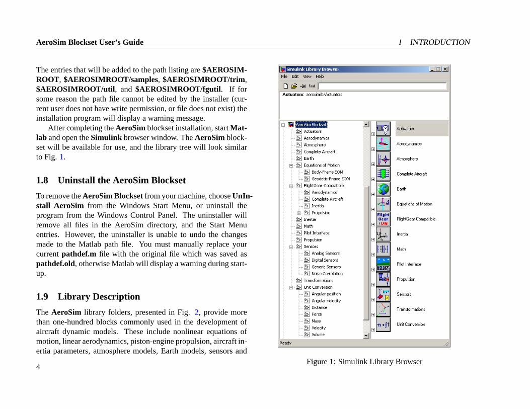
After completing theAeroSim blockset installation, startMat-lab and open theSimulink browser window. TheAeroSim block-set will be available for use, and the library tree will look similarto Fig. 1.
1.8 Uninstall the AeroSim Blockset
To remove theAeroSim Blocksetfrom your machine, chooseUnIn-stall AeroSim from the Windows Start Menu, or uninstall theprogram from the Windows Control Panel. The uninstaller willremove all files in the AeroSim directory, and the Start Menuentries. However, the uninstaller is unable to undo the changesmade to the Matlab path file. You must manually replace yourcurrentpathdef.m file with the original file which was saved aspathdef.old, otherwise Matlab will display a warning during start-up.
1.9 Library Description
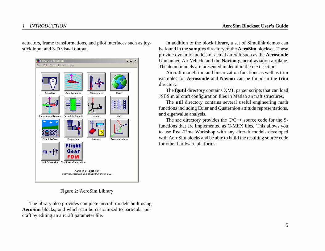
The AeroSim library folders, presented in Fig.2, provide morethan one-hundred blocks commonly used in the development ofaircraft dynamic models. These include nonlinear equations ofmotion, linear aerodynamics, piston-engine propulsion, aircraft in-ertia parameters, atmosphere models, Earth models, sensors and
Figure 1: Simulink Library Browser4
1 INTRODUCTION AeroSim Blockset User’s Guide
actuators, frame transformations, and pilot interfaces such as joy-stick input and 3-D visual output.
Figure 2: AeroSim Library
The library also provides complete aircraft models built usingAeroSim blocks, and which can be customized to particular air-craft by editing an aircraft parameter file.
In addition to the block library, a set of Simulink demos canbe found in thesamplesdirectory of theAeroSim blockset. Theseprovide dynamic models of actual aircraft such as theAerosondeUnmanned Air Vehicle and theNavion general-aviation airplane.The demo models are presented in detail in the next section.
Aircraft model trim and linearization functions as well as trimexamples forAerosondeand Navion can be found in thetrimdirectory.
Thefgutil directory contains XML parser scripts that can loadJSBSim aircraft configuration files in Matlab aircraft structures.
The util directory contains several useful engineering mathfunctions including Euler and Quaternion attitude representations,and eigenvalue analysis.
The src directory provides the C/C++ source code for the S-functions that are implemented as C-MEX files. This allows youto use Real-Time Workshop with any aircraft models developedwith AeroSim blocks and be able to build the resulting source codefor other hardware platforms.
5
AeroSim Blockset User’s Guide 2 AIRCRAFT MODEL DEMOS
2 Aircraft Model Demos
The following Simulink models can be found in thesamplesdi-rectory of the AeroSim library. They illustrate the functionality ofthe AeroSim blockset. The models presented next are using theAerosonde for aircraft dynamics, but similar models exist for theNavion airplane as well.
6
2 AIRCRAFT MODEL DEMOS AeroSim Blockset User’s Guide
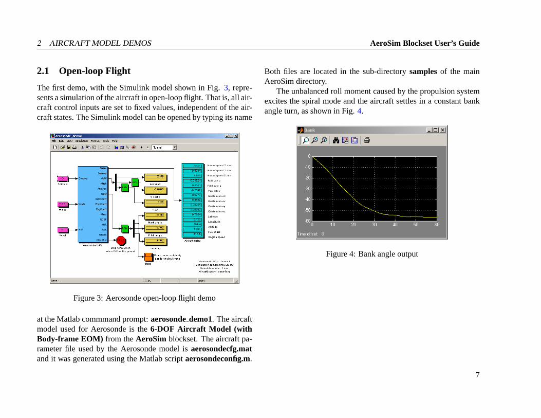
2.1 Open-loop Flight
The first demo, with the Simulink model shown in Fig.3, repre-sents a simulation of the aircraft in open-loop flight. That is, all air-craft control inputs are set to fixed values, independent of the air-craft states. The Simulink model can be opened by typing its name
Figure 3: Aerosonde open-loop flight demo
at the Matlab commmand prompt:aerosondedemo1. The aircaftmodel used for Aerosonde is the6-DOF Aircraft Model (withBody-frame EOM) from theAeroSim blockset. The aircraft pa-rameter file used by the Aerosonde model isaerosondecfg.matand it was generated using the Matlab scriptaerosondeconfig.m.
Both files are located in the sub-directorysamplesof the mainAeroSim directory.
The unbalanced roll moment caused by the propulsion systemexcites the spiral mode and the aircraft settles in a constant bankangle turn, as shown in Fig.4.
Figure 4: Bank angle output
7
AeroSim Blockset User’s Guide 2 AIRCRAFT MODEL DEMOS
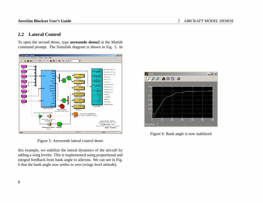
2.2 Lateral Control
To open the second demo, typeaerosondedemo2at the Matlabcommand prompt. The Simulink diagram is shown in Fig.5. In
Figure 5: Aerosonde lateral control demo
this example, we stabilize the lateral dynamics of the aircraft byadding a wing leveler. This is implemented using proportional andintegral feedback from bank angle to ailerons. We can see in Fig.6 that the bank angle now settles to zero (wings level attitude).
Figure 6: Bank angle is now stabilized
8
2 AIRCRAFT MODEL DEMOS AeroSim Blockset User’s Guide
2.3 Airspeed Control
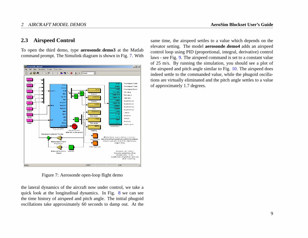
To open the third demo, typeaerosondedemo3 at the Matlabcommand prompt. The Simulink diagram is shown in Fig.7. With
Figure 7: Aerosonde open-loop flight demo
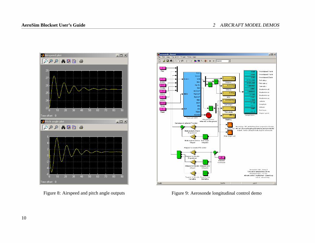
the lateral dynamics of the aircraft now under control, we take aquick look at the longitudinal dynamics. In Fig.8 we can seethe time history of airspeed and pitch angle. The initial phugoidoscillations take approximately 60 seconds to damp out. At the
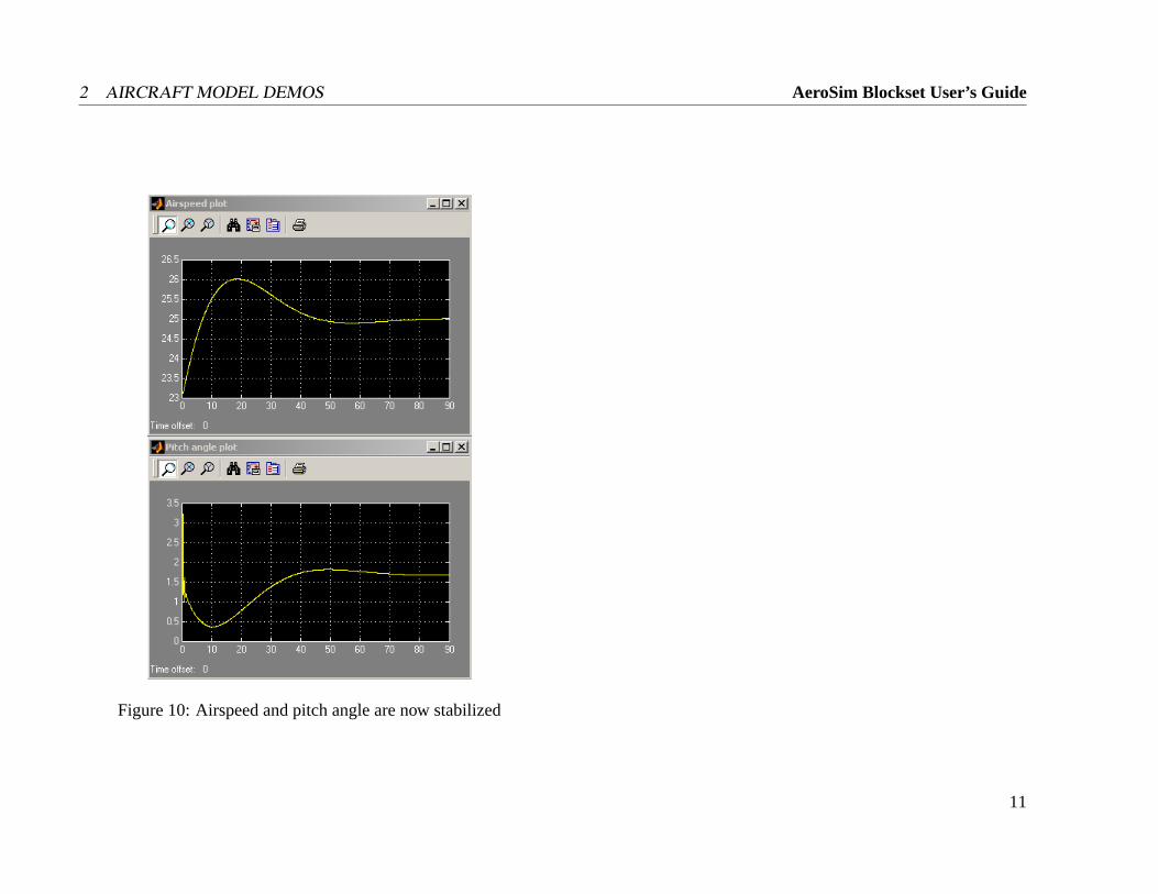
same time, the airspeed settles to a value which depends on theelevator setting. The modelaerosondedemo4adds an airspeedcontrol loop using PID (proportional, integral, derivative) controllaws - see Fig.9. The airspeed command is set to a constant valueof 25 m/s. By running the simulation, you should see a plot ofthe airspeed and pitch angle similar to Fig.10. The airspeed doesindeed settle to the commanded value, while the phugoid oscilla-tions are virtually eliminated and the pitch angle settles to a valueof approximately 1.7 degrees.
9
AeroSim Blockset User’s Guide 2 AIRCRAFT MODEL DEMOS
Figure 8: Airspeed and pitch angle outputs Figure 9: Aerosonde longitudinal control demo
10
2 AIRCRAFT MODEL DEMOS AeroSim Blockset User’s Guide
Figure 10: Airspeed and pitch angle are now stabilized
11
AeroSim Blockset User’s Guide 2 AIRCRAFT MODEL DEMOS
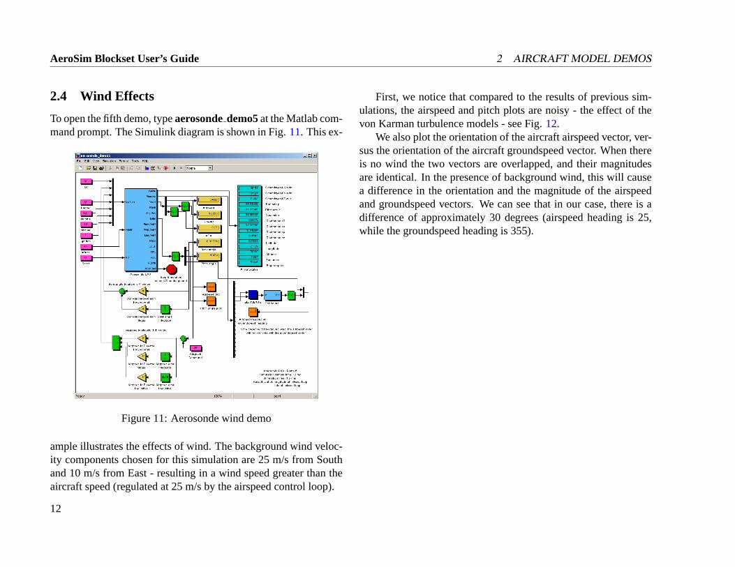
2.4 Wind Effects
To open the fifth demo, typeaerosondedemo5at the Matlab com-mand prompt. The Simulink diagram is shown in Fig.11. This ex-
Figure 11: Aerosonde wind demo
ample illustrates the effects of wind. The background wind veloc-ity components chosen for this simulation are 25 m/s from Southand 10 m/s from East - resulting in a wind speed greater than theaircraft speed (regulated at 25 m/s by the airspeed control loop).
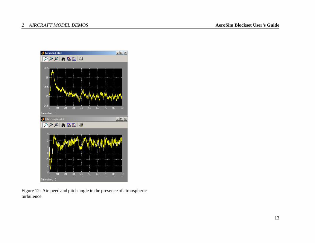
First, we notice that compared to the results of previous sim-ulations, the airspeed and pitch plots are noisy - the effect of thevon Karman turbulence models - see Fig.12.
We also plot the orientation of the aircraft airspeed vector, ver-sus the orientation of the aircraft groundspeed vector. When thereis no wind the two vectors are overlapped, and their magnitudesare identical. In the presence of background wind, this will causea difference in the orientation and the magnitude of the airspeedand groundspeed vectors. We can see that in our case, there is adifference of approximately 30 degrees (airspeed heading is 25,while the groundspeed heading is 355).
12
2 AIRCRAFT MODEL DEMOS AeroSim Blockset User’s Guide
Figure 12: Airspeed and pitch angle in the presence of atmosphericturbulence
13
AeroSim Blockset User’s Guide 2 AIRCRAFT MODEL DEMOS
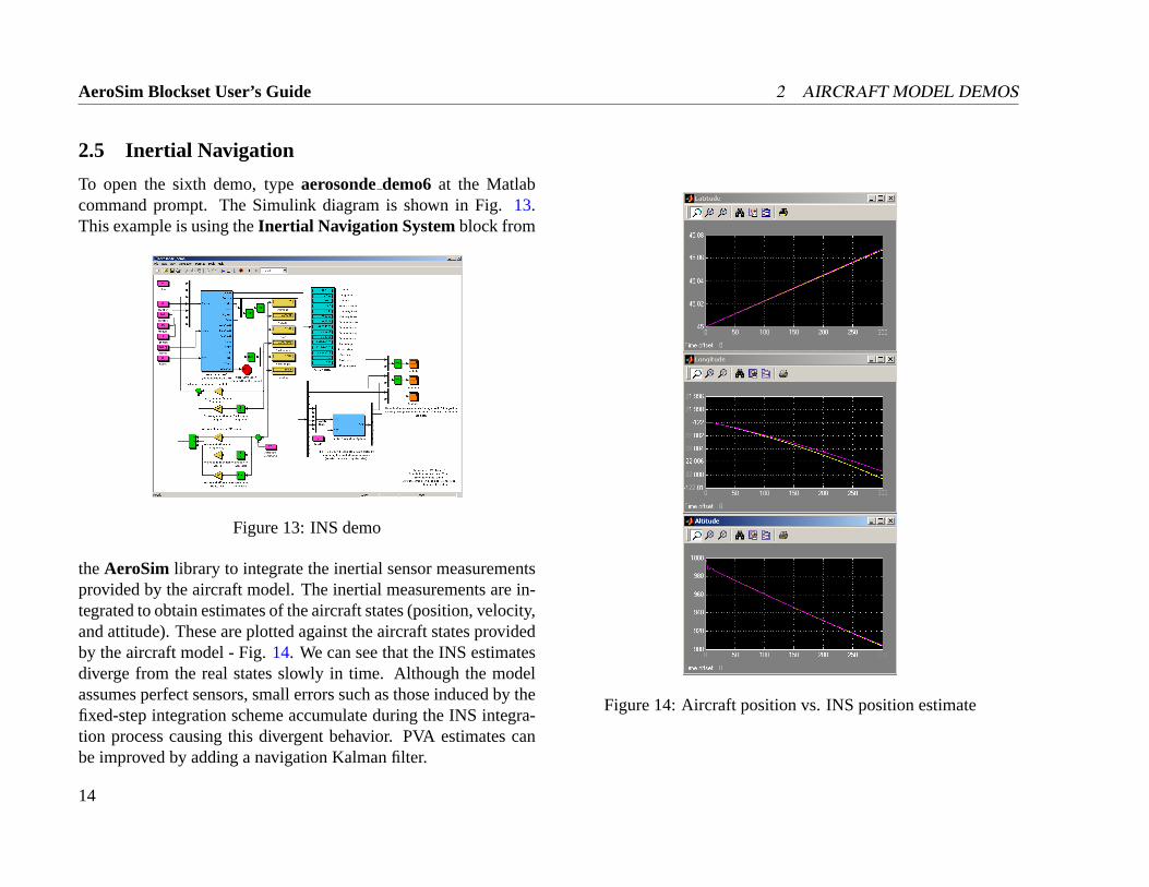
2.5 Inertial Navigation
To open the sixth demo, typeaerosondedemo6 at the Matlabcommand prompt. The Simulink diagram is shown in Fig.13.This example is using theInertial Navigation Systemblock from
Figure 13: INS demo
theAeroSim library to integrate the inertial sensor measurementsprovided by the aircraft model. The inertial measurements are in-tegrated to obtain estimates of the aircraft states (position, velocity,and attitude). These are plotted against the aircraft states providedby the aircraft model - Fig.14. We can see that the INS estimatesdiverge from the real states slowly in time. Although the modelassumes perfect sensors, small errors such as those induced by thefixed-step integration scheme accumulate during the INS integra-tion process causing this divergent behavior. PVA estimates canbe improved by adding a navigation Kalman filter.
Figure 14: Aircraft position vs. INS position estimate
14
2 AIRCRAFT MODEL DEMOS AeroSim Blockset User’s Guide
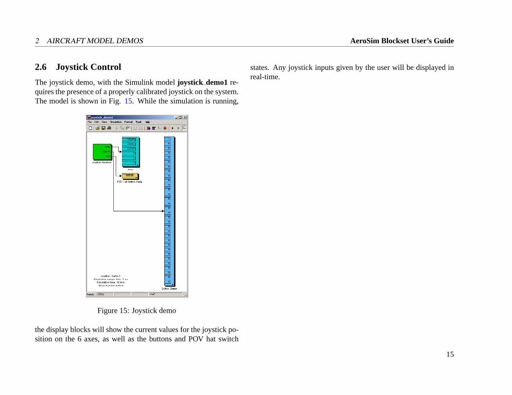
2.6 Joystick Control
The joystick demo, with the Simulink modeljoystick demo1re-quires the presence of a properly calibrated joystick on the system.The model is shown in Fig.15. While the simulation is running,
Figure 15: Joystick demo
the display blocks will show the current values for the joystick po-sition on the 6 axes, as well as the buttons and POV hat switch
states. Any joystick inputs given by the user will be displayed inreal-time.
15
AeroSim Blockset User’s Guide 2 AIRCRAFT MODEL DEMOS
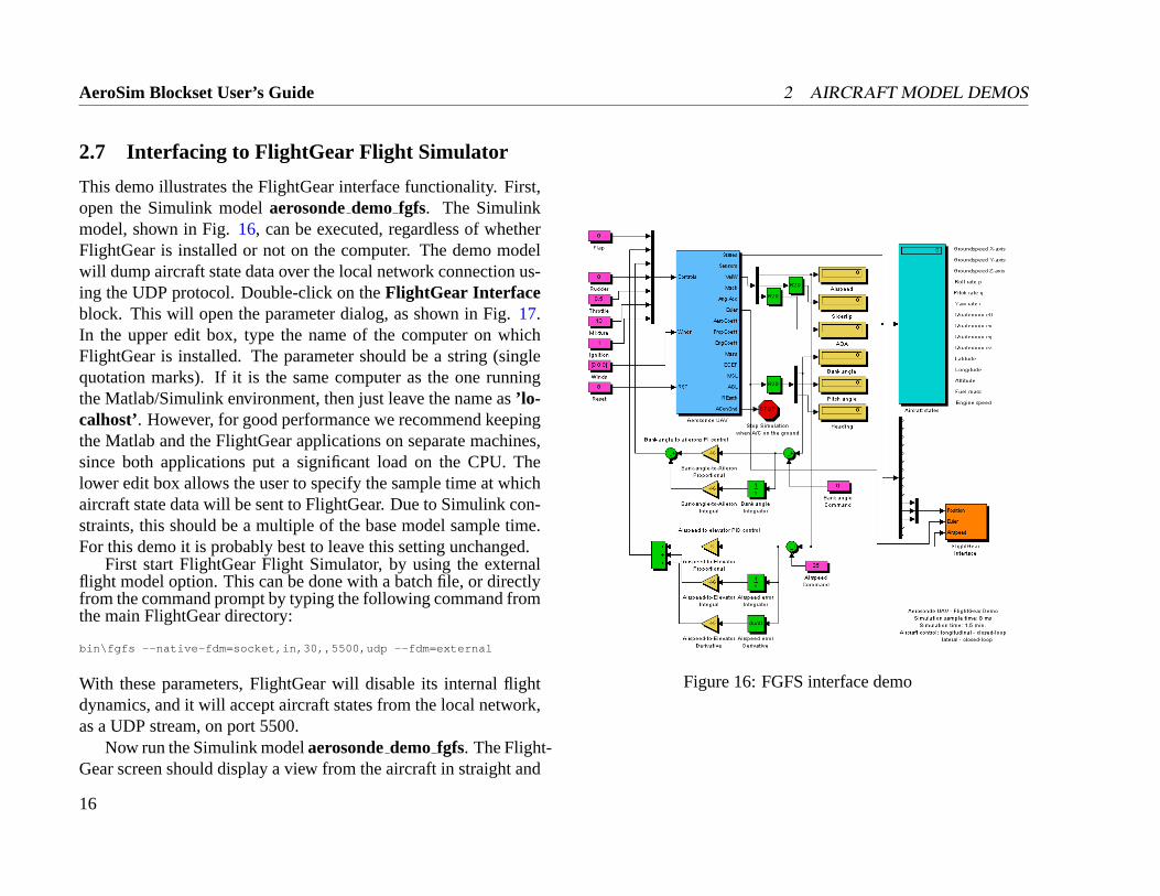
2.7 Interfacing to FlightGear Flight Simulator
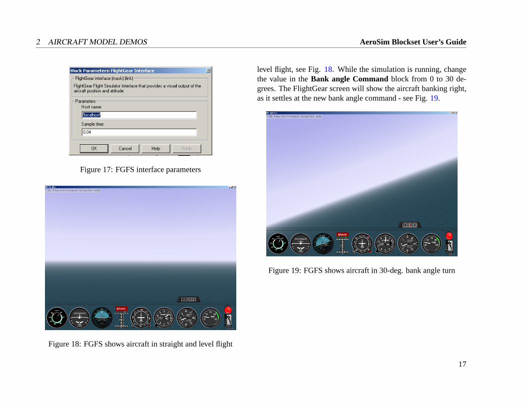
This demo illustrates the FlightGear interface functionality. First,open the Simulink modelaerosondedemo fgfs. The Simulinkmodel, shown in Fig.16, can be executed, regardless of whetherFlightGear is installed or not on the computer. The demo modelwill dump aircraft state data over the local network connection us-ing the UDP protocol. Double-click on theFlightGear Interfaceblock. This will open the parameter dialog, as shown in Fig.17.In the upper edit box, type the name of the computer on whichFlightGear is installed. The parameter should be a string (singlequotation marks). If it is the same computer as the one runningthe Matlab/Simulink environment, then just leave the name as’lo-calhost’. However, for good performance we recommend keepingthe Matlab and the FlightGear applications on separate machines,since both applications put a significant load on the CPU. Thelower edit box allows the user to specify the sample time at whichaircraft state data will be sent to FlightGear. Due to Simulink con-straints, this should be a multiple of the base model sample time.For this demo it is probably best to leave this setting unchanged.
First start FlightGear Flight Simulator, by using the externalflight model option. This can be done with a batch file, or directlyfrom the command prompt by typing the following command fromthe main FlightGear directory:
bin\fgfs --native-fdm=socket,in,30,,5500,udp --fdm=external
With these parameters, FlightGear will disable its internal flightdynamics, and it will accept aircraft states from the local network,as a UDP stream, on port 5500.
Now run the Simulink modelaerosondedemo fgfs. The Flight-Gear screen should display a view from the aircraft in straight and
Figure 16: FGFS interface demo
16
2 AIRCRAFT MODEL DEMOS AeroSim Blockset User’s Guide
Figure 17: FGFS interface parameters
Figure 18: FGFS shows aircraft in straight and level flight
level flight, see Fig.18. While the simulation is running, changethe value in theBank angle Commandblock from 0 to 30 de-grees. The FlightGear screen will show the aircraft banking right,as it settles at the new bank angle command - see Fig.19.
Figure 19: FGFS shows aircraft in 30-deg. bank angle turn
17
AeroSim Blockset User’s Guide 2 AIRCRAFT MODEL DEMOS
2.8 Interfacing to Microsoft Flight Simulator
This demo will present the methodology for interfacing an aircraftdynamic model running in Simulink to a computer runningMi-crosoft Flight Simulator .
1. If using Flight Simulator 2000, install the latest patch (up-date 2b).
2. Unzip fsuipc.zip in a temporary directory and follow theinstallation instructions.
3. Unzip widefs.zip in a temporary directory and follow theinstallation instructions.
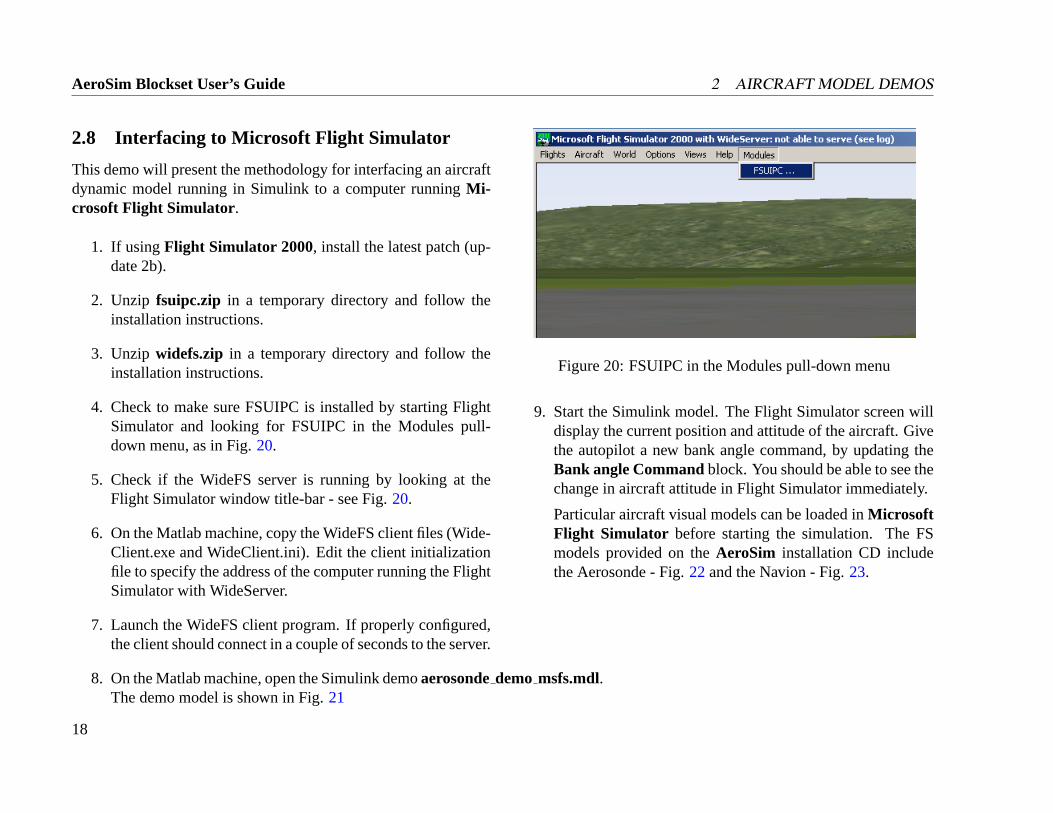
4. Check to make sure FSUIPC is installed by starting FlightSimulator and looking for FSUIPC in the Modules pull-down menu, as in Fig.20.
5. Check if the WideFS server is running by looking at theFlight Simulator window title-bar - see Fig.20.
6. On the Matlab machine, copy the WideFS client files (Wide-Client.exe and WideClient.ini). Edit the client initializationfile to specify the address of the computer running the FlightSimulator with WideServer.
7. Launch the WideFS client program. If properly configured,the client should connect in a couple of seconds to the server.
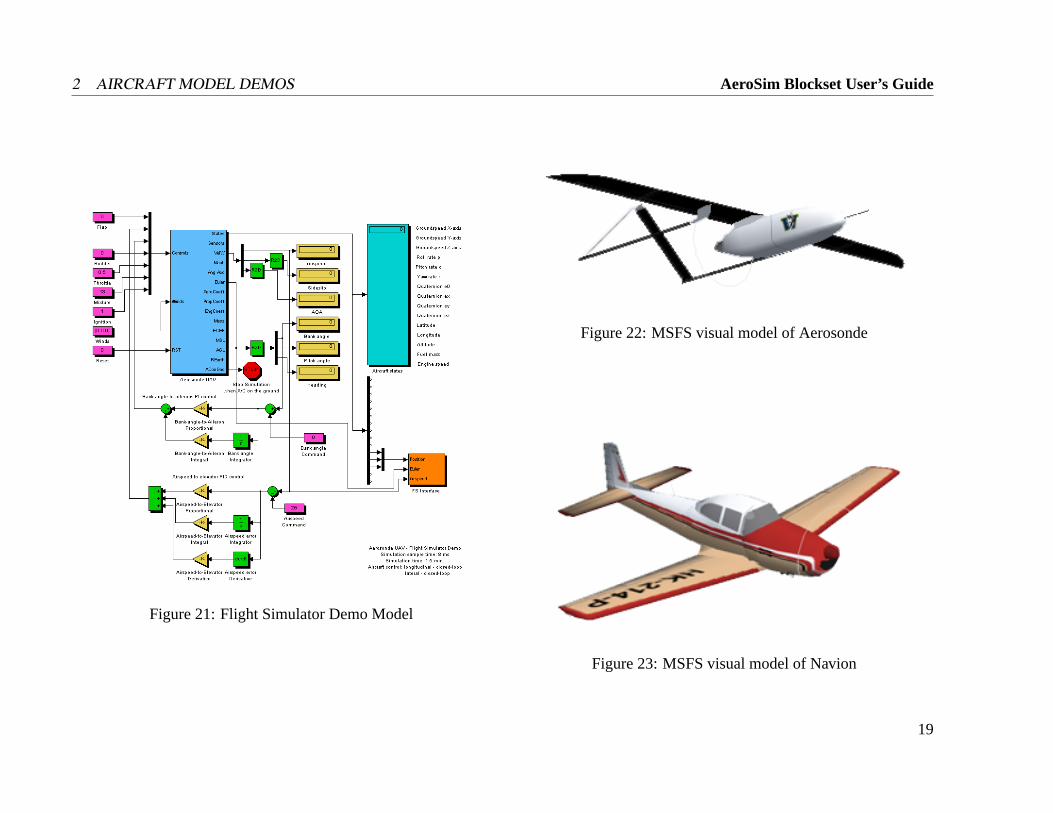
8. On the Matlab machine, open the Simulink demoaerosondedemo msfs.mdl.The demo model is shown in Fig.21
Figure 20: FSUIPC in the Modules pull-down menu
9. Start the Simulink model. The Flight Simulator screen willdisplay the current position and attitude of the aircraft. Givethe autopilot a new bank angle command, by updating theBank angle Commandblock. You should be able to see thechange in aircraft attitude in Flight Simulator immediately.
Particular aircraft visual models can be loaded inMicrosoftFlight Simulator before starting the simulation. The FSmodels provided on theAeroSim installation CD includethe Aerosonde - Fig.22and the Navion - Fig.23.
18
2 AIRCRAFT MODEL DEMOS AeroSim Blockset User’s Guide
Figure 21: Flight Simulator Demo Model
Figure 22: MSFS visual model of Aerosonde
Figure 23: MSFS visual model of Navion
19
AeroSim Blockset User’s Guide 2 AIRCRAFT MODEL DEMOS
2.9 FlightGear Aircraft Demos
The complete models for several aircraft that useJSBSimconfigu-ration files can be found in the AeroSim library. Several ready-to-run demos are also provided in thesamplesdirectory. These are:c172fgdemo.mdl, c182fgdemo.mdl, andc310fgdemo.mdl forthe Cessna-172, 182, and 310 respectively.
Before running any of these Simulink models, make sure toset the correct FlightGear path string in the aircraft model blockparameters, by double-clicking on the aircraft block and editingthe parameterFlightGear path.
20
2 AIRCRAFT MODEL DEMOS AeroSim Blockset User’s Guide
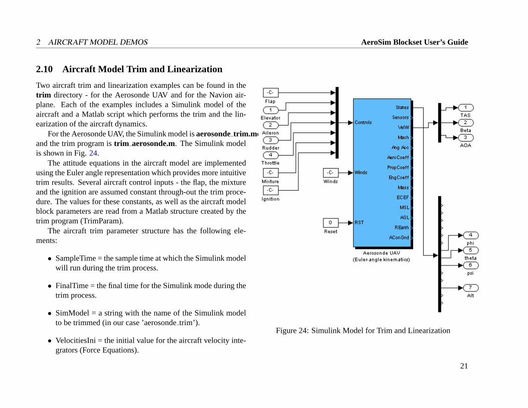
2.10 Aircraft Model Trim and Linearization
Two aircraft trim and linearization examples can be found in thetrim directory - for the Aerosonde UAV and for the Navion air-plane. Each of the examples includes a Simulink model of theaircraft and a Matlab script which performs the trim and the lin-earization of the aircraft dynamics.
For the Aerosonde UAV, the Simulink model isaerosondetrim.mdland the trim program istrim aerosonde.m. The Simulink modelis shown in Fig.24.
The attitude equations in the aircraft model are implementedusing the Euler angle representation which provides more intuitivetrim results. Several aircraft control inputs - the flap, the mixtureand the ignition are assumed constant through-out the trim proce-dure. The values for these constants, as well as the aircraft modelblock parameters are read from a Matlab structure created by thetrim program (TrimParam).
The aircraft trim parameter structure has the following ele-ments:
• SampleTime = the sample time at which the Simulink modelwill run during the trim process.
• FinalTime = the final time for the Simulink mode during thetrim process.
• SimModel = a string with the name of the Simulink modelto be trimmed (in our case ’aerosondetrim’).
• VelocitiesIni = the initial value for the aircraft velocity inte-grators (Force Equations).
Figure 24: Simulink Model for Trim and Linearization
21
AeroSim Blockset User’s Guide 2 AIRCRAFT MODEL DEMOS
• RatesIni = the initial value for the aircraft angular rate inte-grators (Moment Equations).
• AttitudeIni = the initial value for the Euler angle integrators(Kinematic Equations).
• PositionIni = the initial value for the geographic positionintegrators (Navigation Equations).
• FuelIni = the initial value for the fuel mass integrator.
• EngineSpeedIni = the initial value for the engine rotationspeed.
• Airspeed = the airspeed at which the aircraft will be trimmed.
• Altitude = the altitude at which the aircraft will be trimmed.
• BankAngle = the bank (roll) angle at which the aircraft willbe trimmed.
• Elevator = the initial guess for the elevator position at trimcondition.
• Aileron = the initial guess for the aileron position at trimcondition.
• Rudder = the initial guess for the rudder position at trimcondition.
• Throttle = the initial guess for the throttle position at trimcondition.
• Flap = the flap setting at which the aircraft will be trimmed.
• Mixture = the air/fuel mixture at which the aircraft will betrimmed.
• Ignition = choose whether this is a power-on or power-offtrim condition.
• Winds = the background wind vector for which the aircraftwill be trimmed.
• StateIdx = the state order index maps the order of states inthe Simulink diagram to a desired order of states. Oftenthe order in which Matlab considers the states in a Simulinkblock diagram is different that the order we intend to use.In this case, the desired order is [Velocities Rates AttitudePosition Fuel EngineSpeed].
• Options = the Matlab structure which defines the optimiza-tion function options.
• SimOptions = the Matlab structure which defines the simu-lation function options.
• NAircraftStates = the size of the desired aircraft state vector.
• NSimulinkStates = the size of the Simulink model state vec-tor (could be larger since it could include states for otherdynamics which are of no interest for trim (such as the tur-bulence filter states)
The trim and linearization script will create the trim parametersstructure with values provided by the user and with default valuesfor several parameters.
The script performs several steps, as presented below:
22
2 AIRCRAFT MODEL DEMOS AeroSim Blockset User’s Guide
• Set the initial parameters. These include the Simulink modelname and sample time settings as well as default values foraircraft control inputs.
• Identify the order of the aircraft states. The identificationis done by running the Simulink model for a single sampletime with some default initial guesses and reading back theSimulink model state vector to identify the indices for eachof the states of interest.
• Initial guess for the aircraft controls. The procedure firstrequires user input regarding the flight condition at whichthe aircraft is to be trimmed. Once the flight condition iscompletely defined, the Simulink model is run for a limitedamount of time, in an iterative process, and the aircraft con-trol inputs are adjusted each time by proportional feedbackfrom selected model outputs (for example, elevator feed-back is provided by airspeed error, throttle feedback - byaltitude error, and aileron feedback - by bank angle error).The method provides a better initial guess for the next step -the optimization, but the feedback gains are aircraft-specific,therefore the trim script requires some adjustments for eachnew aircraft.
• Perform the aircraft trim. Once a reasonable initial guess forthe aircraft control inputs is obtained, the program will runthe optimization which will accurately trim the aircraft forthe selected flight-condition. The Matlab function used bythis procedure istrim.
• Extract the linear model. Knowing the trim inputs and states,
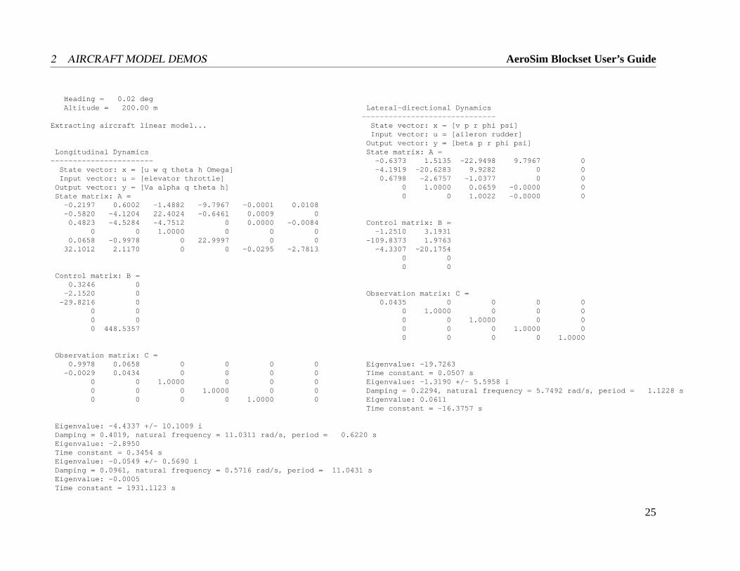
the nonlinear aircraft model is linearized about the trim con-dition, using the Matlab functionlinmod. The resulting lin-ear model is then decoupled into longitudinal and lateral-directional plants; this procedure is valid only if the aircraftis trimmed for straight and level flight. At the end of thelinearization procedure, a simple eigenvalue analysis of thelongitudinal and lateral-directional dynamics is performed.
To illustrate the process, we will trim the Aerosonde model fora typical flight condition (Va = 23m/s, h = 200m, φ = 0). By run-ning the trim programtrim aerosonde.mwe obtain the followingoutput:
Setting initial trim parameters...
The Simulink modelaerosonde_trim.mdl will be trimmed.
Identifying the order of the Simulink model states...done.
Choose flight condition:--------------------------Trim airspeed [m/s]: 23
Trim altitude [m]: 200
Trim bank angle[rad]: 0
Fuel mass [kg]: 2
Flap setting [frac]: 0
Computing the initial estimates for the trim inputs...
Iteration # 1, Airsp err = 3.86 m/s, Alt err = -23.96 m, phierr = -15.80 deg.
Iteration # 2, Airsp err = 0.88 m/s, Alt err = 12.95 m, phi err= -24.39 deg.
23
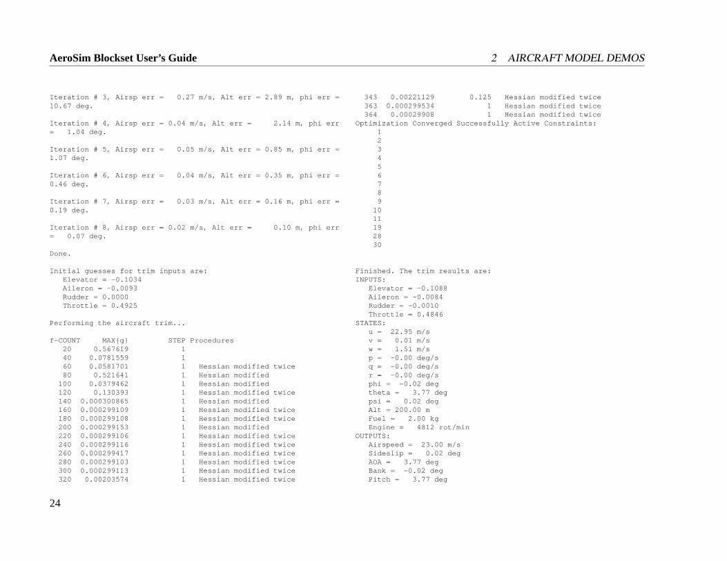
AeroSim Blockset User’s Guide 2 AIRCRAFT MODEL DEMOS
Iteration # 3, Airsp err = 0.27 m/s, Alt err = 2.89 m, phi err =10.67 deg.
Iteration # 4, Airsp err = 0.04 m/s, Alt err = 2.14 m, phi err= 1.04 deg.
Iteration # 5, Airsp err = 0.05 m/s, Alt err = 0.85 m, phi err =1.07 deg.
Iteration # 6, Airsp err = 0.04 m/s, Alt err = 0.35 m, phi err =0.46 deg.
Iteration # 7, Airsp err = 0.03 m/s, Alt err = 0.16 m, phi err =0.19 deg.
Iteration # 8, Airsp err = 0.02 m/s, Alt err = 0.10 m, phi err= 0.07 deg.
Done.
Initial guesses for trim inputs are:Elevator = -0.1034Aileron = -0.0093Rudder = 0.0000Throttle = 0.4925
Performing the aircraft trim...
f-COUNT MAXg STEP Procedures20 0.567619 140 0.0781559 160 0.0581701 1 Hessian modified twice80 0.521641 1 Hessian modified
100 0.0379462 1 Hessian modified120 0.130393 1 Hessian modified twice140 0.000300865 1 Hessian modified160 0.000299109 1 Hessian modified twice180 0.000299108 1 Hessian modified twice200 0.000299153 1 Hessian modified220 0.000299106 1 Hessian modified twice240 0.000299116 1 Hessian modified twice260 0.000299417 1 Hessian modified twice280 0.000299103 1 Hessian modified twice300 0.000299113 1 Hessian modified twice320 0.00203574 1 Hessian modified twice
343 0.00221129 0.125 Hessian modified twice363 0.000299534 1 Hessian modified twice364 0.00029908 1 Hessian modified twice
Optimization Converged Successfully Active Constraints:123456789
1011192830
Finished. The trim results are:INPUTS:
Elevator = -0.1088Aileron = -0.0084Rudder = -0.0010Throttle = 0.4846
STATES:u = 22.95 m/sv = 0.01 m/sw = 1.51 m/sp = -0.00 deg/sq = -0.00 deg/sr = -0.00 deg/sphi = -0.02 degtheta = 3.77 degpsi = 0.02 degAlt = 200.00 mFuel = 2.00 kgEngine = 4812 rot/min
OUTPUTS:Airspeed = 23.00 m/sSideslip = 0.02 degAOA = 3.77 degBank = -0.02 degPitch = 3.77 deg
24
2 AIRCRAFT MODEL DEMOS AeroSim Blockset User’s Guide
Heading = 0.02 degAltitude = 200.00 m
Extracting aircraft linear model...
Longitudinal Dynamics-----------------------
State vector: x = [u w q theta h Omega]Input vector: u = [elevator throttle]
Output vector: y = [Va alpha q theta h]State matrix: A =
-0.2197 0.6002 -1.4882 -9.7967 -0.0001 0.0108-0.5820 -4.1204 22.4024 -0.6461 0.0009 0
0.4823 -4.5284 -4.7512 0 0.0000 -0.00840 0 1.0000 0 0 0
0.0658 -0.9978 0 22.9997 0 032.1012 2.1170 0 0 -0.0295 -2.7813
Control matrix: B =0.3246 0
-2.1520 0-29.8216 0
0 00 00 448.5357
Observation matrix: C =0.9978 0.0658 0 0 0 0
-0.0029 0.0434 0 0 0 00 0 1.0000 0 0 00 0 0 1.0000 0 00 0 0 0 1.0000 0
Eigenvalue: -4.4337 +/- 10.1009 iDamping = 0.4019, natural frequency = 11.0311 rad/s, period = 0.6220 sEigenvalue: -2.8950Time constant = 0.3454 sEigenvalue: -0.0549 +/- 0.5690 iDamping = 0.0961, natural frequency = 0.5716 rad/s, period = 11.0431 sEigenvalue: -0.0005Time constant = 1931.1123 s
Lateral-directional Dynamics------------------------------
State vector: x = [v p r phi psi]Input vector: u = [aileron rudder]
Output vector: y = [beta p r phi psi]State matrix: A =
-0.6373 1.5135 -22.9498 9.7967 0-4.1919 -20.6283 9.9282 0 0
0.6798 -2.6757 -1.0377 0 00 1.0000 0.0659 -0.0000 00 0 1.0022 -0.0000 0
Control matrix: B =-1.2510 3.1931
-109.8373 1.9763-4.3307 -20.1754
0 00 0
Observation matrix: C =0.0435 0 0 0 0
0 1.0000 0 0 00 0 1.0000 0 00 0 0 1.0000 00 0 0 0 1.0000
Eigenvalue: -19.7263Time constant = 0.0507 sEigenvalue: -1.3190 +/- 5.5958 iDamping = 0.2294, natural frequency = 5.7492 rad/s, period = 1.1228 sEigenvalue: 0.0611Time constant = -16.3757 s
25
AeroSim Blockset User’s Guide 3 SETTING-UP AND RUNNING AN AIRCRAFT MODEL
3 Setting-up and Running an Aircraft Model
This chapter outlines the pre-built aircraft models that are providedin theAeroSim blockset. These can be customized by setting theaircraft aerodynamic, propulsion, and inertia properties in an air-craft parameter file. The general architecture of the complete air-craft model blocks is also presented. Finally, special issues suchas interfacing the Simulink models with Flight Simulator are dis-cussed.
26
3 SETTING-UP AND RUNNING AN AIRCRAFT MODEL AeroSim Blockset User’s Guide
3.1 Aircraft Model Examples
The following aircraft examples are included in theAeroSimblock-set:
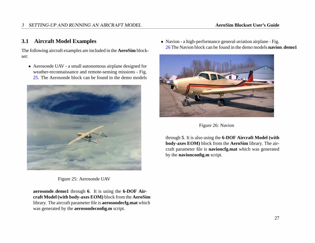
• Aerosonde UAV - a small autonomous airplane designed forweather-reconnaissance and remote-sensing missions - Fig.25. The Aerosonde block can be found in the demo models
Figure 25: Aerosonde UAV
aerosondedemo1 through6. It is using the6-DOF Air-craft Model (with body-axes EOM) block from theAeroSimlibrary. The aircraft parameter file isaerosondecfg.matwhichwas generated by theaerosondeconfig.mscript.
• Navion - a high-performance general-aviation airplane - Fig.26The Navion block can be found in the demo modelsnavion demo1
Figure 26: Navion
through5. It is also using the6-DOF Aircraft Model (withbody-axes EOM)block from theAeroSim library. The air-craft parameter file isnavioncfg.mat which was generatedby thenavionconfig.mscript.
27
AeroSim Blockset User’s Guide 3 SETTING-UP AND RUNNING AN AIRCRAFT MODEL
3.2 Building an aircraft configuration
A new aircraft parameter file can be generated from a custom Mat-lab script. To create this script, you would need to open the tem-plate aircraft configuration scriptconfig template.mwhich can befound in thesamplesdirectory, and specify the aircraft aerody-namic, propulsion and inertia parameters.
By running this script at the Matlab command prompt, a newaircraft parameter file of the formfilename.matwill be created.The file name can then be used in any of the complete aircraftblocks available in theAeroSim library.
The first variable that should be specified is the name of the air-craft parameter file that will be generated. Type the chosen nameof your aircraft parameter file, as a string, without the .mat exten-sion:
% Insert the name of the MAT-file that will be generated% (without .mat extension)cfgmatfile = ’myairplanecfg’;
3.2.1 Conventions
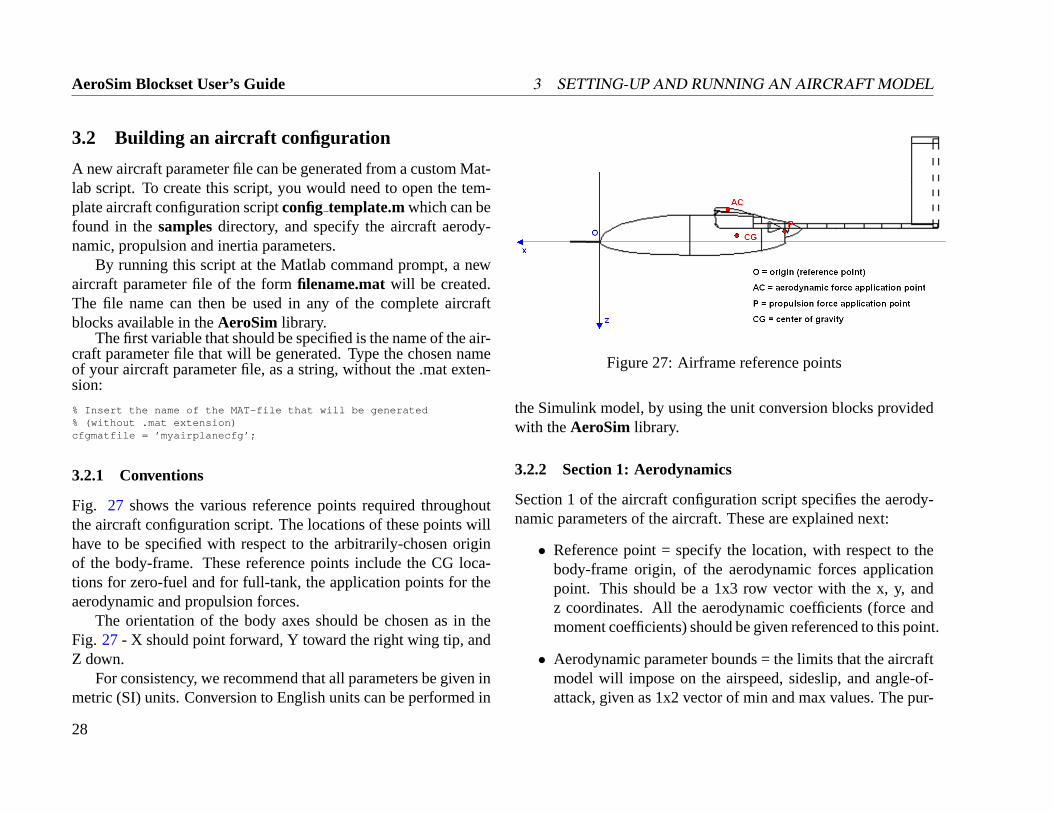
Fig. 27 shows the various reference points required throughoutthe aircraft configuration script. The locations of these points willhave to be specified with respect to the arbitrarily-chosen originof the body-frame. These reference points include the CG loca-tions for zero-fuel and for full-tank, the application points for theaerodynamic and propulsion forces.
The orientation of the body axes should be chosen as in theFig. 27 - X should point forward, Y toward the right wing tip, andZ down.
For consistency, we recommend that all parameters be given inmetric (SI) units. Conversion to English units can be performed in
Figure 27: Airframe reference points
the Simulink model, by using the unit conversion blocks providedwith theAeroSim library.
3.2.2 Section 1: Aerodynamics
Section 1 of the aircraft configuration script specifies the aerody-namic parameters of the aircraft. These are explained next:
• Reference point = specify the location, with respect to thebody-frame origin, of the aerodynamic forces applicationpoint. This should be a 1x3 row vector with the x, y, andz coordinates. All the aerodynamic coefficients (force andmoment coefficients) should be given referenced to this point.
• Aerodynamic parameter bounds = the limits that the aircraftmodel will impose on the airspeed, sideslip, and angle-of-attack, given as 1x2 vector of min and max values. The pur-
28
3 SETTING-UP AND RUNNING AN AIRCRAFT MODEL AeroSim Blockset User’s Guide
pose of using these limits is to keep the outputs of the aero-dynamic model within the linear region. The componentbuild-up method implemented by the aerodynamic modelin the AeroSim library uses first order terms, therefore theaerodynamic model will provide acceptable results only inthe linear aerodynamics conditions (small angles).
• Aerodynamic reference parameters = the reference param-eters for which the aerodynamic coefficients were normal-ized. These include the reference wing chord, the wing span,and the reference wing area.
• Lift coefficient terms. The lift coefficient is computed usingthe expression (1).
CL = CL0 +CαL ·α+C
δ fL ·δ f +Cδe
L ·δe+
+ c2Va
(Cα
L · α+CqL ·q)+CM
L ·M(1)
• Drag coefficient terms. The drag coefficient is computedusing the expression (2).
CD = CD0 + (CL−CL0)2
πeAR +Cδ fD ·δ f +Cδe
D ·δe+
+CδaD ·δa +Cδr
D ·δr +CML ·M
(2)
• Side force coefficient terms. The side force coefficient iscomputed using the expression (3).
CY = CβY ·β+Cδa
Y ·δa +CδrY ·δr+
+ b2Va
(Cp
Y · p+CrY · r) (3)
• Pitch moment coefficient terms. The pitch moment coeffi-cient is computed using the expression (4).
Cm = Cm0 +Cαm ·α+C
δ fm ·δ f +Cδe
m ·δe+
+ c2Va
(Cα
m · α+Cqm ·q
)+CM
m ·M(4)
• Roll moment coefficient terms. The roll moment coefficientis computed using the expression (5).
Cl = Cβl ·β+Cδa
l ·δa +Cδrl ·δr+
+ b2Va
(Cp
l · p+Crl · r) (5)
• Yaw moment coefficient terms. The yaw moment coefficientis computed using the expression (6).
Cn = Cβn ·β+Cδa
n ·δa +Cδrn ·δr+
+ b2Va
(Cp
n · p+Crn · r) (6)
3.2.3 Section 2: Propeller
The second section of the aircraft configuration script specifies thegeometry and aerodynamic performance of the propeller.
• Propeller hub location = the position of the propulsion forceand moment application point, given with respect to the body-frame origin. The location is specified as a 1x3 row vectorof x, y, and z coordinates.
29
AeroSim Blockset User’s Guide 3 SETTING-UP AND RUNNING AN AIRCRAFT MODEL
• Advance ratio. The aerodynamic performance of the pro-peller should be given as a look-up table of propeller coef-ficients (CP and CT) as functions of the propeller advanceratio. This variable specifies the advance ratio vector whichcorresponds to the look-up table.
• Coefficient of thrust. The vector of coefficients of thrust forthe advance ratios given above (the vector should have thesame size).
• Coefficient of power. The vector of coefficients of power forthe advance ratios given above (the vector should have thesame size).
• Propeller radius = the radius of the propeller is used by thepropulsion model to compute the force and torque from thenormalized coefficients. These loads are computed as fol-lows:
Fp =4π2ρR4Ω2CT (7)
Mp =− 4π3ρR5Ω2CP (8)
• Propeller inertia = the propeller moment of inertia is usedby the propulsion equation of motion (dynamics) to solvefor the current rotation speed.
3.2.4 Section 3: Engine
The third section of the aircraft configuration scripts allows theuser to specify the engine characteristics. All engine data is givenat sea-level. The engine model will correct the data for altitude
effects. For a normally-aspirated general aviation piston engine,this includes the following parameters:
• RPM = the vector of engine speeds for which the engine datais given, in rotations-per-minute. All engine parameters arespecified as 2-D look-up tables (functions of engine speedand intake manifold pressure).
• MAP = the vector of manifold pressures for which the en-gine data is given, in kilo-pascals.
• Fuel flow = the sea-level fuel flow as a function of RPMand MAP. The number of rows in the matrix should matchthe size of the RPM vector, the number of columns shouldmatch the size of the MAP vector.
• Power = the engine power at sea-level, as a function of RPMand MAP. The number of rows in the matrix should matchthe size of the RPM vector, the number of columns shouldmatch the size of the MAP vector.
• Sea-level atmospheric conditions = the sea-level atmosphericconditions, including pressure in Pascals and temperature indegrees Kelvin, for which the engine data above is given.
• Engine shaft inertia = the moment of inertia of the rotatingparts of the engine. This is added to the propeller inertiaand used in the propulsion equation of motion to computethe current engine speed. Generally, the engine shaft inertiais significantly lower than that of the propeller, and it can beneglected without any major effects over the aircraft dynam-ics.
30
3 SETTING-UP AND RUNNING AN AIRCRAFT MODEL AeroSim Blockset User’s Guide
3.2.5 Section 4: Inertia
The fourth section of the aircraft configuration script specifies theinertia parameters of the aircraft: mass, CG location, and momentsof inertia.
• Empty aircraft mass = the mass of the aircraft without fuel.
• Gross aircraft mass = the mass of the aircraft with the fueltank full.
• CG empty = the position of the center of gravity for the air-craft without fuel. This is provided as a 1x3 vector of x, y, zcoordinates with respect to the origin.
• CG gross = the position of the center of gravity for the air-craft with full fuel tank. This is provided as a 1x3 vector ofx, y, z coordinates with respect to the origin.
• Empty moments of inertia = the moments of inertia of theaircraft without fuel. These are provided as a 1x4 vector ofmoment of inertia about body axes -Jx, Jy, Jz, andJxz. Formost aircraft the inertia cross-productsJxy and Jyz can beneglected because of the symmetry about the x-z plane.
• Gross moments of inertia = the moments of inertia of the air-craft with full fuel tank. These are provided as a 1x4 vectorof moment of inertia about body axes -Jx, Jy, Jz, andJxz.
3.2.6 Section 5: Other parameters
In the last section of the aircraft configuration script, the user canset other, less important parameters. At this point, the only vari-
able that can be edited is the calendar date used by the World Mag-netic Model to compute the magnetic field at aircraft location. Thedate is specified as a 1x3 vector of day, month, and year.
31
AeroSim Blockset User’s Guide 3 SETTING-UP AND RUNNING AN AIRCRAFT MODEL
3.3 The pre-built Aircraft Models
Once the editing of the aircraft configuration script is completed, itshould be saved with a unique name, for examplemyairplanecon-fig.m.
By executing the scriptmyairplaneconfig.mat the Matlab com-mand prompt, an aircraft configuration file -myairplanecfg.matwill be created in the present working directory.
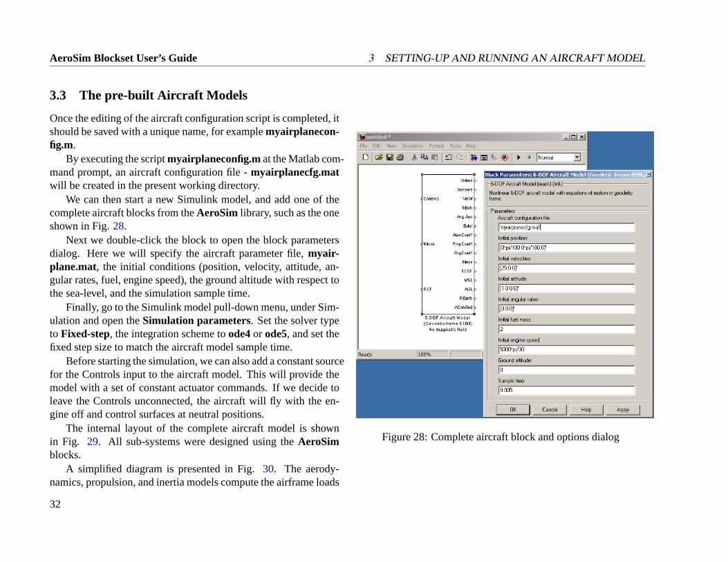
We can then start a new Simulink model, and add one of thecomplete aircraft blocks from theAeroSim library, such as the oneshown in Fig.28.
Next we double-click the block to open the block parametersdialog. Here we will specify the aircraft parameter file,myair-plane.mat, the initial conditions (position, velocity, attitude, an-gular rates, fuel, engine speed), the ground altitude with respect tothe sea-level, and the simulation sample time.
Finally, go to the Simulink model pull-down menu, under Sim-ulation and open theSimulation parameters. Set the solver typeto Fixed-step, the integration scheme toode4or ode5, and set thefixed step size to match the aircraft model sample time.
Before starting the simulation, we can also add a constant sourcefor the Controls input to the aircraft model. This will provide themodel with a set of constant actuator commands. If we decide toleave the Controls unconnected, the aircraft will fly with the en-gine off and control surfaces at neutral positions.
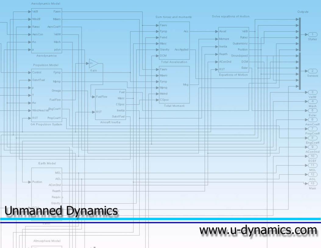
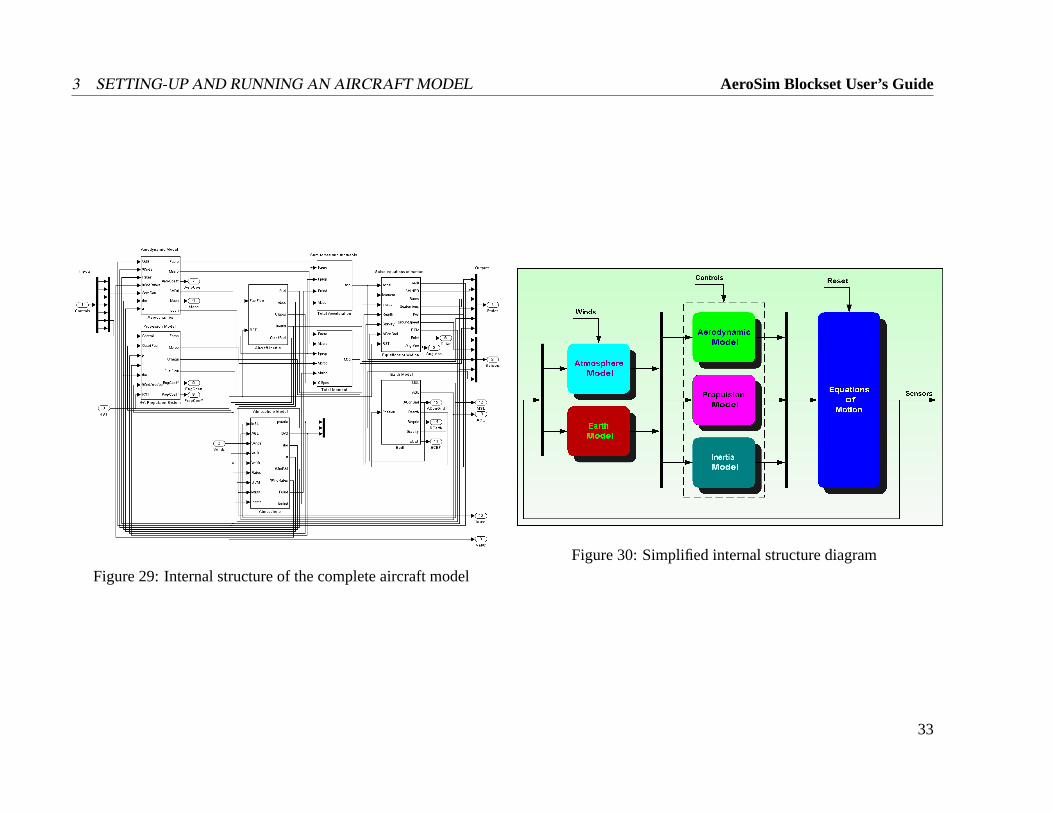
The internal layout of the complete aircraft model is shownin Fig. 29. All sub-systems were designed using theAeroSimblocks.
A simplified diagram is presented in Fig.30. The aerody-namics, propulsion, and inertia models compute the airframe loads
Figure 28: Complete aircraft block and options dialog
32
3 SETTING-UP AND RUNNING AN AIRCRAFT MODEL AeroSim Blockset User’s Guide
Figure 29: Internal structure of the complete aircraft modelFigure 30: Simplified internal structure diagram
33
AeroSim Blockset User’s Guide 3 SETTING-UP AND RUNNING AN AIRCRAFT MODEL
(forces and moments) as functions of control inputs and environ-ment (atmosphere and Earth) effects. The resulting accelerationsare then integrated by the Equations of Motion to obtain the air-craft states (position, velocity, attitude, angular velocities). Theaircraft states then will affect the output of the environment blocksat the next iteration (for example altitude changes result in atmo-spheric pressure changes, latitude and longitude variations resultin gravity variations). Also, the aircraft states are used in the com-putation of sensor outputs (GPS, inertial measurements, etc.).
34
3 SETTING-UP AND RUNNING AN AIRCRAFT MODEL AeroSim Blockset User’s Guide
3.4 Using FlightGear Aircraft Configuration Files
FlightGear is an open-source multi-platform cooperative flight sim-ulator project. Source code for the entire project is available andlicensed under the GNU General Public License. The goal ofthe FlightGear project is to create a sophisticated flight simula-tor framework for use in research or academic environments, forthe development and pursuit of other interesting flight simulationideas, and as an end-user application. For more information pleasevisit the main FlightGear website, athttp://www.flightgear.org .
Initially, the FlightGear project used theLaRCSim flight dy-namics code for the simulation of aircraft dynamics. However,the LaRCSim software was inflexible in defining the aircraft pa-rameters (any change to the default aircraft - Navion - parametersrequired manual editing of the LaRCSim source code). Due to thisfact, several new flight dynamic codes for FlightGear were createdand are in various stages of development. Of these, the best knownproject isJSBSim, an open-source flight dynamics model whichcan be used either from FlightGear or independent of the visualinterface. For more information about the JSBSim project, visitthe main JSBSim website, athttp://jsbsim.sourceforge.net.
3.4.1 The JSBSim XML Configuration File
The main strength of JSBSim is that it provides flexibility to theflight dynamics developer by accepting aircraft configurations asXML files which are structured and easy to read. The lack ofstandards for exchange of aircraft models in the flight simulation
community is well known and poses problems since most aircraftdevelopment projects involve several contractors and these wouldhave to exchange flight dynamic models on a regular basis. Theopen-source community, and JSBSim in particular, have taken thefirst steps in establishing an XML-based standard for aircraft mod-els.
A detailed and evolving document that describes the JSBSimconfiguration or definition files can be found on the main JSBSimwebsite. A brief presentation of these files is done next.
There are three types of JSBSim definition files:
1. Aircraft Definition File, which describes the airframe ge-ometry and inertia parameters, the aerodynamics, the flightcontrol system, and which types of engine(s) and thruster(s)the aircraft has.
2. Engine Definition File, which describes the properties of aspecific engine. At this time JSBSim supports piston androcket engines, but turbine engine models are under devel-opment.
3. Thruster Definition File, which describes the properties of aspecific thruster. At this time JSBSim provides models forpropellers and nozzles.
This layout permits development of aircraft models in a struc-tured fashion in which the same aircraft can be easily fitted with adifferent engine or propeller. The engine and thruster componentscan be reused for new aircraft configurations.
The Aircraft Definition File is structured in the following sub-sections, defined as xml tags:
35
AeroSim Blockset User’s Guide 3 SETTING-UP AND RUNNING AN AIRCRAFT MODEL
• METRICS, which describes the aircraft geometry and inertiaparameters
• UNDERCARRIAGE, which describes the landing gear andground contact points,
• PROPULSION, which specifies which engine(s) and thruster(s)are used, what is their location in the aircraft coordinates. Italso specifies the fuel/oxydizer tanks.
• FLIGHT CONTROL, which specifies the aircraft flight con-trol laws.
• AERODYNAMICS, which includes all of the aerodynamiccoefficients and scaling parameters required for computingthe aerodynamic forces and moments.
• OUTPUT, which specifies what parameters of the flight dy-namics model the program will output.
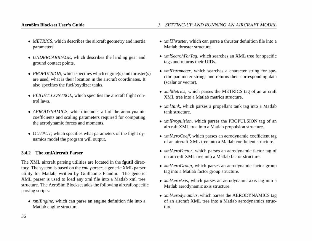
3.4.2 The xmlAircraft Parser
The XML aircraft parsing utilities are located in thefgutil direc-tory. The system is based on thexml parser, a generic XML parserutility for Matlab, written by Guillaume Flandin. The genericXML parser is used to load any xml file into a Matlab xml treestructure. The AeroSim Blockset adds the following aircraft-specificparsing scripts:
• xmlEngine, which can parse an engine definition file into aMatlab engine structure.
• xmlThruster, which can parse a thruster definition file into aMatlab thruster structure.
• xmlSearchForTag, which searches an XML tree for specifictags and returns their UIDs.
• xmlParameter, which searches a character string for spe-cific parameter strings and returns their corresponding data(scalar or vector).
• xmlMetrics, which parses the METRICS tag of an aircraftXML tree into a Matlab metrics structure.
• xmlTank, which parses a propellant tank tag into a Matlabtank structure.
• xmlPropulsion, which parses the PROPULSION tag of anaircraft XML tree into a Matlab propulsion structure.
• xmlAeroCoeff, which parses an aerodynamic coefficient tagof an aircraft XML tree into a Matlab coefficient structure.
• xmlAeroFactor, which parses an aerodynamic factor tag ofon aircraft XML tree into a Matlab factor structure.
• xmlAeroGroup, which parses an aerodynamic factor grouptag into a Matlab factor group structure.
• xmlAeroAxis, which parses an aerodynamic axis tag into aMatlab aerodynamic axis structure.
• xmlAerodynamics, which parses the AERODYNAMICS tagof an aircraft XML tree into a Matlab aerodynamics struc-ture.
36
3 SETTING-UP AND RUNNING AN AIRCRAFT MODEL AeroSim Blockset User’s Guide
• xmlAircraft, which is the main aircraft definition file parser.The function reads an aircraft definition file along with itsengine and thruster definition files and parses the completeaircraft model into a Matlab aircraft structure. The aircraftstructure is documented in the next subsection.
• AircraftUnitConv, which is an unit conversion function thatprocesses a Matlab aircraft structure returned byxmlAircraft(JSBSim uses English units) and converts all parameters tometric units.
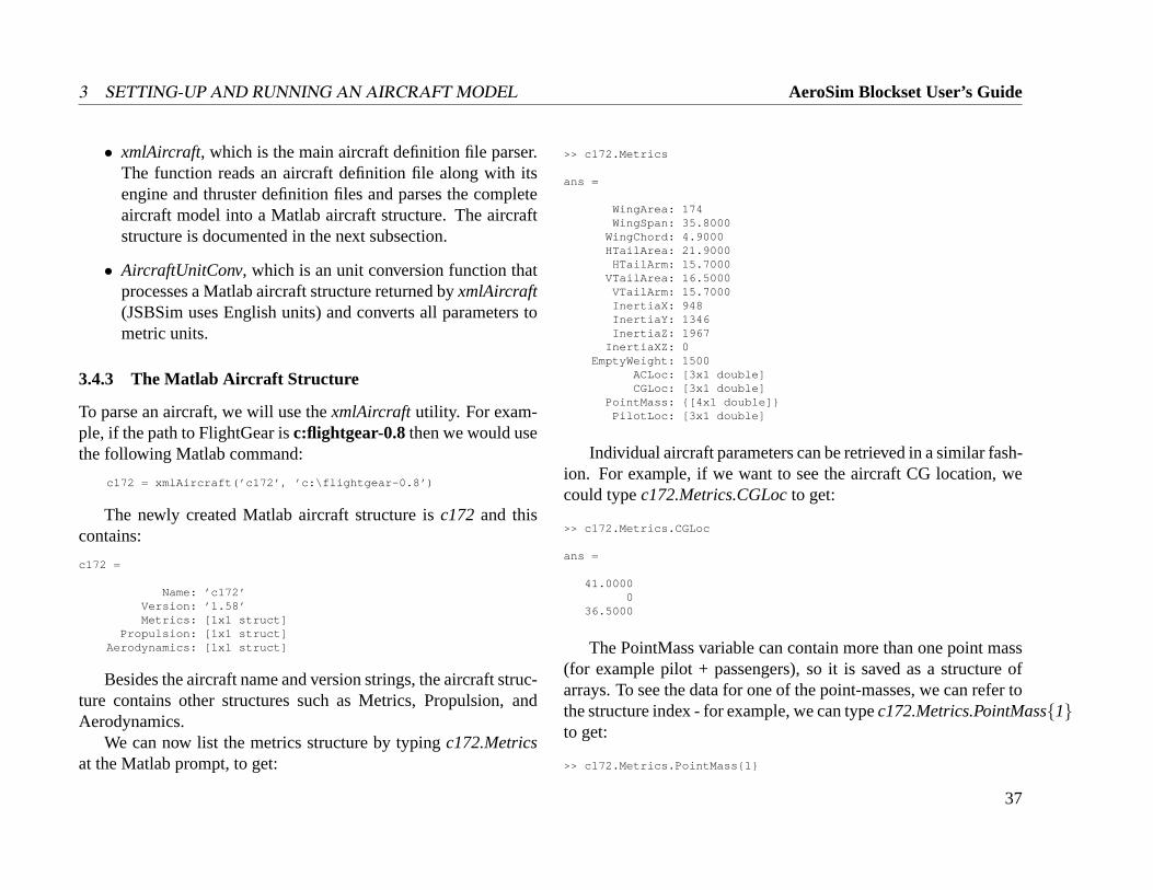
3.4.3 The Matlab Aircraft Structure
To parse an aircraft, we will use thexmlAircraft utility. For exam-ple, if the path to FlightGear isc:flightgear-0.8then we would usethe following Matlab command:
c172 = xmlAircraft(’c172’, ’c:\flightgear-0.8’)
The newly created Matlab aircraft structure isc172 and thiscontains:
c172 =
Name: ’c172’Version: ’1.58’Metrics: [1x1 struct]
Propulsion: [1x1 struct]Aerodynamics: [1x1 struct]
Besides the aircraft name and version strings, the aircraft struc-ture contains other structures such as Metrics, Propulsion, andAerodynamics.
We can now list the metrics structure by typingc172.Metricsat the Matlab prompt, to get:
>> c172.Metrics
ans =
WingArea: 174WingSpan: 35.8000
WingChord: 4.9000HTailArea: 21.9000
HTailArm: 15.7000VTailArea: 16.5000
VTailArm: 15.7000InertiaX: 948InertiaY: 1346InertiaZ: 1967
InertiaXZ: 0EmptyWeight: 1500
ACLoc: [3x1 double]CGLoc: [3x1 double]
PointMass: [4x1 double]PilotLoc: [3x1 double]
Individual aircraft parameters can be retrieved in a similar fash-ion. For example, if we want to see the aircraft CG location, wecould typec172.Metrics.CGLocto get:
>> c172.Metrics.CGLoc
ans =
41.00000
36.5000
The PointMass variable can contain more than one point mass(for example pilot + passengers), so it is saved as a structure ofarrays. To see the data for one of the point-masses, we can refer tothe structure index - for example, we can typec172.Metrics.PointMass1to get:
>> c172.Metrics.PointMass1
37
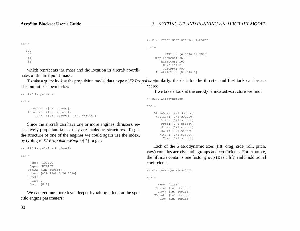
AeroSim Blockset User’s Guide 3 SETTING-UP AND RUNNING AN AIRCRAFT MODEL
ans =
18036
-1424
which represents the mass and the location in aircraft coordi-nates of the first point-mass.
To take a quick look at the propulsion model data, typec172.Propulsion.The output is shown below:
>> c172.Propulsion
ans =
Engine: [1x1 struct]Thruster: [1x1 struct]
Tank: [1x1 struct] [1x1 struct]
Since the aircraft can have one or more engines, thrusters, re-spectively propellant tanks, they are loaded as structures. To getthe structure of one of the engines we could again use the index,by typingc172.Propulsion.Engine1 to get:
>> c172.Propulsion.Engine1
ans =
Name: ’IO360C’Type: ’PISTON’
Param: [1x1 struct]Loc: [-19.7000 0 26.6000]
Pitch: 0Yaw: 0
Feed: [0 1]
We can get one more level deeper by taking a look at the spe-cific engine parameters:
>> c172.Propulsion.Engine1.Param
ans =
MAPLim: [6.5000 28.5000]Displacement: 360
MaxPower: 160NCycles: 2IdleRPM: 900
ThrottleLim: [0.2000 1]
Similarly, the data for the thruster and fuel tank can be ac-cessed.
If we take a look at the aerodynamics sub-structure we find:
>> c172.Aerodynamics
ans =
AlphaLim: [2x1 double]HystLim: [2x1 double]
Lift: [1x1 struct]Drag: [1x1 struct]Side: [1x1 struct]Roll: [1x1 struct]
Pitch: [1x1 struct]Yaw: [1x1 struct]
Each of the 6 aerodynamic axes (lift, drag, side, roll, pitch,yaw) contains aerodynamic groups and coefficients. For example,the lift axis contains one factor group (Basic lift) and 3 additionalcoefficients:
>> c172.Aerodynamics.Lift
ans =
Name: ’LIFT’Basic: [1x1 struct]
CLDe: [1x1 struct]CLadot: [1x1 struct]
CLq: [1x1 struct]
38
3 SETTING-UP AND RUNNING AN AIRCRAFT MODEL AeroSim Blockset User’s Guide
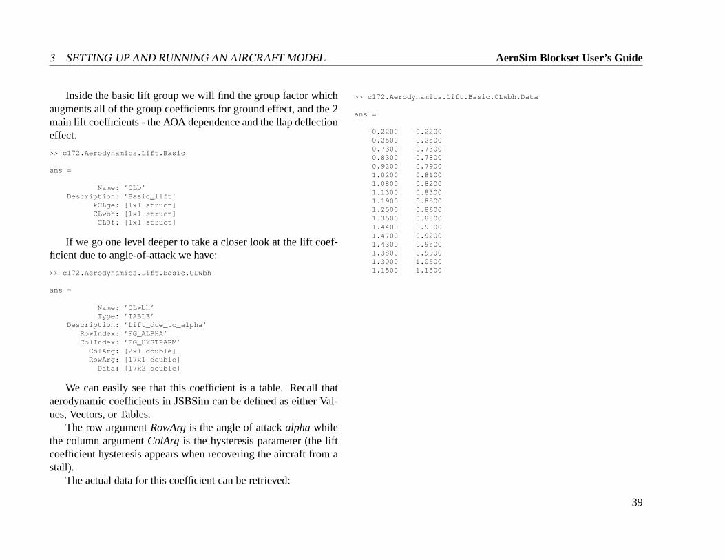
Inside the basic lift group we will find the group factor whichaugments all of the group coefficients for ground effect, and the 2main lift coefficients - the AOA dependence and the flap deflectioneffect.
>> c172.Aerodynamics.Lift.Basic
ans =
Name: ’CLb’Description: ’Basic_lift’
kCLge: [1x1 struct]CLwbh: [1x1 struct]
CLDf: [1x1 struct]
If we go one level deeper to take a closer look at the lift coef-ficient due to angle-of-attack we have:
>> c172.Aerodynamics.Lift.Basic.CLwbh
ans =
Name: ’CLwbh’Type: ’TABLE’
Description: ’Lift_due_to_alpha’RowIndex: ’FG_ALPHA’ColIndex: ’FG_HYSTPARM’
ColArg: [2x1 double]RowArg: [17x1 double]
Data: [17x2 double]
We can easily see that this coefficient is a table. Recall thataerodynamic coefficients in JSBSim can be defined as either Val-ues, Vectors, or Tables.
The row argumentRowArgis the angle of attackalphawhilethe column argumentColArg is the hysteresis parameter (the liftcoefficient hysteresis appears when recovering the aircraft from astall).
The actual data for this coefficient can be retrieved:
>> c172.Aerodynamics.Lift.Basic.CLwbh.Data
ans =
-0.2200 -0.22000.2500 0.25000.7300 0.73000.8300 0.78000.9200 0.79001.0200 0.81001.0800 0.82001.1300 0.83001.1900 0.85001.2500 0.86001.3500 0.88001.4400 0.90001.4700 0.92001.4300 0.95001.3800 0.99001.3000 1.05001.1500 1.1500
39
AeroSim Blockset User’s Guide 3 SETTING-UP AND RUNNING AN AIRCRAFT MODEL
3.5 Additional Matlab Utilities
The directoryutil contains two small Matlab functions.
• eigparamcomputes the damping, period, natural and dampedfrequencies of a complex eigenvalue. The function is usedby the aircraft trim and linearization scripts to display thecharacteristics of the linear aircraft models.
• euler2quatcomputes the quaternion vector corresponding tothe Euler angle representation. The function can be usedto compute the initial quaternions required for an aircraftmodel based on the initial aircraft attitude expressed in Eulerangles.
40
4 BLOCK REFERENCE AeroSim Blockset User’s Guide
4 Block Reference
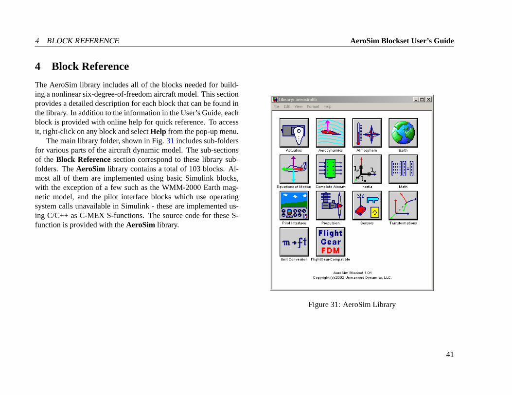
The AeroSim library includes all of the blocks needed for build-ing a nonlinear six-degree-of-freedom aircraft model. This sectionprovides a detailed description for each block that can be found inthe library. In addition to the information in the User’s Guide, eachblock is provided with online help for quick reference. To accessit, right-click on any block and selectHelp from the pop-up menu.
The main library folder, shown in Fig.31 includes sub-foldersfor various parts of the aircraft dynamic model. The sub-sectionsof the Block Referencesection correspond to these library sub-folders. TheAeroSim library contains a total of 103 blocks. Al-most all of them are implemented using basic Simulink blocks,with the exception of a few such as the WMM-2000 Earth mag-netic model, and the pilot interface blocks which use operatingsystem calls unavailable in Simulink - these are implemented us-ing C/C++ as C-MEX S-functions. The source code for these S-function is provided with theAeroSim library.
Figure 31: AeroSim Library
41
AeroSim Blockset User’s Guide 4 BLOCK REFERENCE
4.1 Actuators
TheActuators folder contains generic models of electro-mechanicalactuators used in flight control systems. Although a fully-functionalaircraft dynamic model can be created without making use of theseblocks, the actuator models are very useful for testing the stabilityand performance of airplane-autopilot closed-loop systems.
42
4 BLOCK REFERENCE AeroSim Blockset User’s Guide
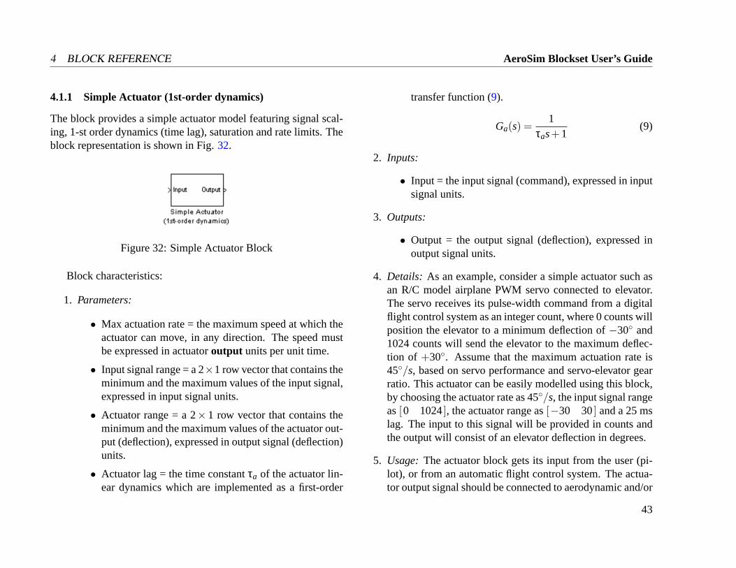
4.1.1 Simple Actuator (1st-order dynamics)
The block provides a simple actuator model featuring signal scal-ing, 1-st order dynamics (time lag), saturation and rate limits. Theblock representation is shown in Fig.32.
Figure 32: Simple Actuator Block
Block characteristics:
1. Parameters:
• Max actuation rate = the maximum speed at which theactuator can move, in any direction. The speed mustbe expressed in actuatoroutput units per unit time.
• Input signal range = a 2×1 row vector that contains theminimum and the maximum values of the input signal,expressed in input signal units.
• Actuator range = a 2×1 row vector that contains theminimum and the maximum values of the actuator out-put (deflection), expressed in output signal (deflection)units.
• Actuator lag = the time constantτa of the actuator lin-ear dynamics which are implemented as a first-order
transfer function (9).
Ga(s) =1
τas+1(9)
2. Inputs:
• Input = the input signal (command), expressed in inputsignal units.
3. Outputs:
• Output = the output signal (deflection), expressed inoutput signal units.
4. Details: As an example, consider a simple actuator such asan R/C model airplane PWM servo connected to elevator.The servo receives its pulse-width command from a digitalflight control system as an integer count, where 0 counts willposition the elevator to a minimum deflection of−30 and1024 counts will send the elevator to the maximum deflec-tion of +30. Assume that the maximum actuation rate is45/s, based on servo performance and servo-elevator gearratio. This actuator can be easily modelled using this block,by choosing the actuator rate as 45/s, the input signal rangeas[0 1024], the actuator range as[−30 30] and a 25 mslag. The input to this signal will be provided in counts andthe output will consist of an elevator deflection in degrees.
5. Usage:The actuator block gets its input from the user (pi-lot), or from an automatic flight control system. The actua-tor output signal should be connected to aerodynamic and/or
43
AeroSim Blockset User’s Guide 4 BLOCK REFERENCE
propulsion blocks that compute the forces and moments ap-plied to the airframe due to the actuator deflection.
44
4 BLOCK REFERENCE AeroSim Blockset User’s Guide
4.1.2 Simple Actuator (2nd-order dynamics)
The block provides a simple actuator model featuring signal scal-ing, 2-nd order dynamics, saturation and rate limits. The blockrepresentation is shown in Fig.33.
Figure 33: Simple Actuator Block
Block characteristics:
1. Parameters:
• Max actuation rate = the maximum speed at which theactuator can move, in any direction. The speed mustbe expressed in actuatoroutput units per unit time.
• Input signal range = a 2×1 row vector that contains theminimum and the maximum values of the input signal,expressed in input signal units.
• Actuator range = a 2×1 row vector that contains theminimum and the maximum values of the actuator out-put (deflection), expressed in output signal (deflection)units.
• Bandwidth = the actuator bandwidthb at a gaing =−3dB and phaseφ = −90. The 2-nd order transfer
function is implemented as in (10).
Ga(s) =ω2
n
s2 +2ζωns+ω2n
(10)
whereωn = 2πb andζ = 1210
−g20 .
2. Inputs:
• Input = the input signal (command), expressed in inputsignal units.
3. Outputs:
• Output = the output signal (deflection), expressed inoutput signal units.
4. Details: The functionality of this block is similar to thatof the Simple Actuator with 1st-order dynamics (previoussubsection).
5. Usage:The actuator block gets its input from the user (pi-lot), or from an automatic flight control system. The actua-tor output signal should be connected to aerodynamic and/orpropulsion blocks that compute the forces and moments ap-plied to the airframe due to the actuator deflection.
45
AeroSim Blockset User’s Guide 4 BLOCK REFERENCE
4.1.3 D/A Converter
The D/A Converterblock converts the digital signal with a spec-ified resolution to an analog voltage within a specified voltagerange. The block is pictured in Fig.34.
Figure 34: D/A Converter Block
Block characteristics:
1. Parameters:
• Voltage range = a 1×2 vector containing the minimumand maximum values of the output voltage.
• Resolution = the number of bits of resolution, whichdetermine the number of counts available on the speci-fied voltage range. For example, a 10-bit converter willprovide 210 = 1024 counts.
• Sample time = the time interval at which the digitalsignal is provided.
2. Inputs:
• Digital = the digital signal, in counts.
3. Outputs:
• Analog = the analog input signal, in volts.
4. Details: The block includes scale-factor conversion fromcounts to volts, saturation limits on the output signal.
5. Usage:The block can be used to convert actuator commandsprovided by a digital flight control system to analog actuatordeflections.
46
4 BLOCK REFERENCE AeroSim Blockset User’s Guide
4.2 Aerodynamics
TheAerodynamics library folder contains all the blocks requiredto develop a simple aerodynamic model of the aircraft. The ap-proach taken in theAeroSim library involves linear aerodynamicsin which the aerodynamic force and moment coefficients are com-puted using linear combinations of aerodynamic derivatives.
47
AeroSim Blockset User’s Guide 4 BLOCK REFERENCE
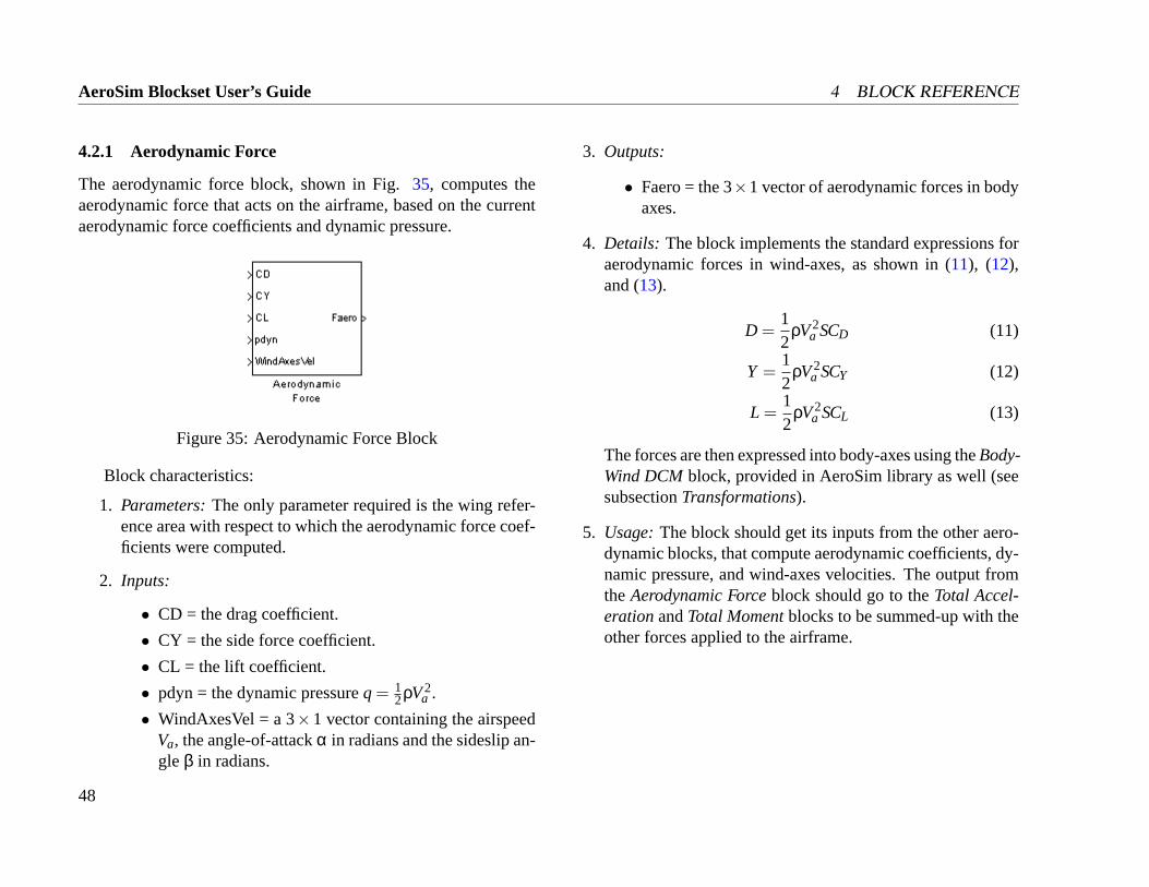
4.2.1 Aerodynamic Force
The aerodynamic force block, shown in Fig.35, computes theaerodynamic force that acts on the airframe, based on the currentaerodynamic force coefficients and dynamic pressure.
Figure 35: Aerodynamic Force Block
Block characteristics:
1. Parameters:The only parameter required is the wing refer-ence area with respect to which the aerodynamic force coef-ficients were computed.
2. Inputs:
• CD = the drag coefficient.
• CY = the side force coefficient.
• CL = the lift coefficient.
• pdyn = the dynamic pressureq = 12ρV2
a .
• WindAxesVel = a 3×1 vector containing the airspeedVa, the angle-of-attackα in radians and the sideslip an-gle β in radians.
3. Outputs:
• Faero = the 3×1 vector of aerodynamic forces in bodyaxes.
4. Details: The block implements the standard expressions foraerodynamic forces in wind-axes, as shown in (11), (12),and (13).
D =12
ρV2a SCD (11)
Y =12
ρV2a SCY (12)
L =12
ρV2a SCL (13)
The forces are then expressed into body-axes using theBody-Wind DCMblock, provided in AeroSim library as well (seesubsectionTransformations).
5. Usage:The block should get its inputs from the other aero-dynamic blocks, that compute aerodynamic coefficients, dy-namic pressure, and wind-axes velocities. The output fromtheAerodynamic Forceblock should go to theTotal Accel-erationandTotal Momentblocks to be summed-up with theother forces applied to the airframe.
48
4 BLOCK REFERENCE AeroSim Blockset User’s Guide
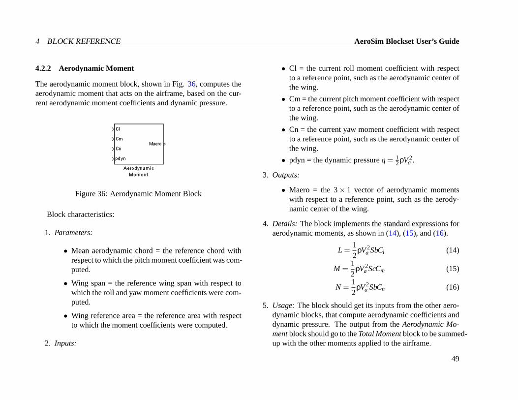
4.2.2 Aerodynamic Moment
The aerodynamic moment block, shown in Fig.36, computes theaerodynamic moment that acts on the airframe, based on the cur-rent aerodynamic moment coefficients and dynamic pressure.
Figure 36: Aerodynamic Moment Block
Block characteristics:
1. Parameters:
• Mean aerodynamic chord = the reference chord withrespect to which the pitch moment coefficient was com-puted.
• Wing span = the reference wing span with respect towhich the roll and yaw moment coefficients were com-puted.
• Wing reference area = the reference area with respectto which the moment coefficients were computed.
2. Inputs:
• Cl = the current roll moment coefficient with respectto a reference point, such as the aerodynamic center ofthe wing.
• Cm = the current pitch moment coefficient with respectto a reference point, such as the aerodynamic center ofthe wing.
• Cn = the current yaw moment coefficient with respectto a reference point, such as the aerodynamic center ofthe wing.
• pdyn = the dynamic pressureq = 12ρV2
a .
3. Outputs:
• Maero = the 3× 1 vector of aerodynamic momentswith respect to a reference point, such as the aerody-namic center of the wing.
4. Details: The block implements the standard expressions foraerodynamic moments, as shown in (14), (15), and (16).
L =12
ρV2a SbCl (14)
M =12
ρV2a ScCm (15)
N =12
ρV2a SbCn (16)
5. Usage:The block should get its inputs from the other aero-dynamic blocks, that compute aerodynamic coefficients anddynamic pressure. The output from theAerodynamic Mo-mentblock should go to theTotal Momentblock to be summed-up with the other moments applied to the airframe.
49
AeroSim Blockset User’s Guide 4 BLOCK REFERENCE
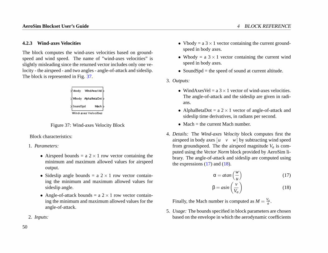
4.2.3 Wind-axes Velocities
The block computes the wind-axes velocities based on ground-speed and wind speed. The name of ”wind-axes velocities” isslightly misleading since the returned vector includes only one ve-locity - the airspeed - and two angles - angle-of-attack and sideslip.The block is represented in Fig.37.
Figure 37: Wind-axes Velocity Block
Block characteristics:
1. Parameters:
• Airspeed bounds = a 2× 1 row vector containing theminimum and maximum allowed values for airspeedoutput.
• Sideslip angle bounds = a 2× 1 row vector contain-ing the minimum and maximum allowed values forsideslip angle.
• Angle-of-attack bounds = a 2×1 row vector contain-ing the minimum and maximum allowed values for theangle-of-attack.
2. Inputs:
• Vbody = a 3×1 vector containing the current ground-speed in body axes.
• Wbody = a 3× 1 vector containing the current windspeed in body axes.
• SoundSpd = the speed of sound at current altitude.
3. Outputs:
• WindAxesVel = a 3×1 vector of wind-axes velocities.The angle-of-attack and the sideslip are given in radi-ans.
• AlphaBetaDot = a 2×1 vector of angle-of-attack andsideslip time derivatives, in radians per second.
• Mach = the current Mach number.
4. Details: The Wind-axes Velocityblock computes first theairspeed in body axes[u v w] by subtracting wind speedfrom groundspeed. The the airspeed magnitudeVa is com-puted using theVector Normblock provided by AeroSim li-brary. The angle-of-attack and sideslip are computed usingthe expressions (17) and (18).
α = atan(w
u
)(17)
β = asin
(v
Va
)(18)
Finally, the Mach number is computed asM = Vaa .
5. Usage:The bounds specified in block parameters are chosenbased on the envelope in which the aerodynamic coefficients
50
4 BLOCK REFERENCE AeroSim Blockset User’s Guide
are expected to provide reasonably accurate aerodynamicbehavior. For example, if the aerodynamic coefficients willbe computed using the linear aerodynamic models providedin AeroSim library, then for a typical General Aviation air-plane we would bound the angle-of attack to, let’s say,−3
to 10, and the side-slip angle to±5. If the aerodynamiccoefficients are provided as look-up tables, then we wouldbound the airflow angles such that table limits are not ex-ceeded. The airspeed should be bounded according to theaircraft’s flight envelope.
The groundspeed components in body axes are provided bythe Forcesblock in Equations of Motion. The wind speedcomponents are provided by theBackground WindandTur-bulenceblocks inAtmosphere. The speed of sound is pro-vided by theStandard Atmosphereblock inAtmosphere. Thewind-axes velocities, the time derivatives of airflow angles,and the Mach number are used by many otherAerodynamicsandPropulsionblocks.
51
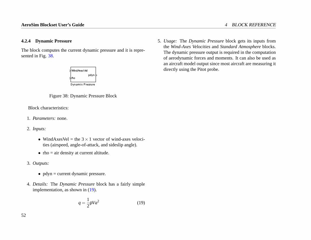
AeroSim Blockset User’s Guide 4 BLOCK REFERENCE
4.2.4 Dynamic Pressure
The block computes the current dynamic pressure and it is repre-sented in Fig.38.
Figure 38: Dynamic Pressure Block
Block characteristics:
1. Parameters:none.
2. Inputs:
• WindAxesVel = the 3×1 vector of wind-axes veloci-ties (airspeed, angle-of-attack, and sideslip angle).
• rho = air density at current altitude.
3. Outputs:
• pdyn = current dynamic pressure.
4. Details: The Dynamic Pressureblock has a fairly simpleimplementation, as shown in (19).
q =12
ρVa2 (19)
5. Usage: The Dynamic Pressureblock gets its inputs fromthe Wind-Axes VelocitiesandStandard Atmosphereblocks.The dynamic pressure output is required in the computationof aerodynamic forces and moments. It can also be used asan aircraft model output since most aircraft are measuring itdirectly using the Pitot probe.
52
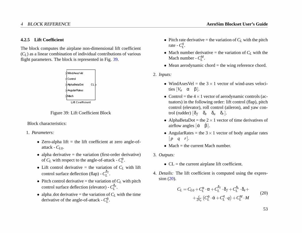
4 BLOCK REFERENCE AeroSim Blockset User’s Guide
4.2.5 Lift Coefficient
The block computes the airplane non-dimensional lift coefficient(CL) as a linear combination of individual contributions of variousflight parameters. The block is represented in Fig.39.
Figure 39: Lift Coefficient Block
Block characteristics:
1. Parameters:
• Zero-alpha lift = the lift coefficient at zero angle-of-attack -CL0.
• alpha derivative = the variation (first-order derivative)of CL with respect to the angle-of-attack -Cα
L .
• Lift control derivative = the variation ofCL with liftcontrol surface deflection (flap) -C
δ fL .
• Pitch control derivative = the variation ofCL with pitchcontrol surface deflection (elevator) -Cδe
L .
• alphadot derivative = the variation ofCL with the timederivative of the angle-of-attack -Cα
L .
• Pitch rate derivative = the variation ofCL with the pitchrate -Cq
L.
• Mach number derivative = the variation ofCL with theMach number -CM
L .
• Mean aerodynamic chord = the wing reference chord.
2. Inputs:
• WindAxesVel = the 3×1 vector of wind-axes veloci-ties[Va α β ].
• Control = the 4×1 vector of aerodynamic controls (ac-tuators) in the following order: lift control (flap), pitchcontrol (elevator), roll control (aileron), and yaw con-trol (rudder)[δ f δe δa δr ].
• AlphaBetaDot = the 2×1 vector of time derivatives ofairflow angles[ α β ].
• AngularRates = the 3×1 vector of body angular rates[ p q r].
• Mach = the current Mach number.
3. Outputs:
• CL = the current airplane lift coefficient.
4. Details: The lift coefficient is computed using the expres-sion (20).
CL = CL0 +CαL ·α+C
δ fL ·δ f +Cδe
L ·δe+
+ c2Va
(Cα
L · α+CqL ·q)+CM
L ·M(20)
53
AeroSim Blockset User’s Guide 4 BLOCK REFERENCE
5. Usage:The inputs should be provided byWind-axes Veloci-tiesblock in Aerodynamics, Momentsblock in Equations ofMotion. Control input is provided by manual or automaticpilot. Block output is used byAerodynamic Forceblock.
54
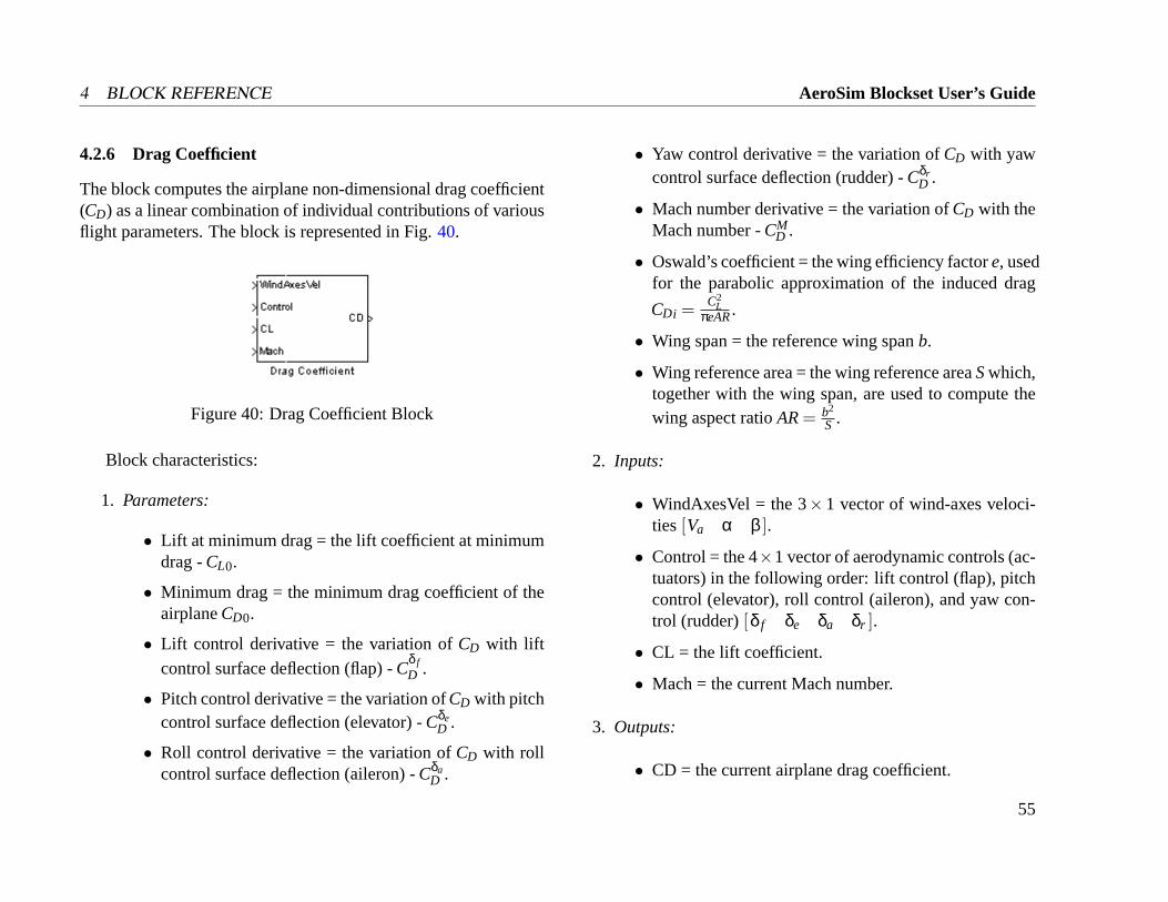
4 BLOCK REFERENCE AeroSim Blockset User’s Guide
4.2.6 Drag Coefficient
The block computes the airplane non-dimensional drag coefficient(CD) as a linear combination of individual contributions of variousflight parameters. The block is represented in Fig.40.
Figure 40: Drag Coefficient Block
Block characteristics:
1. Parameters:
• Lift at minimum drag = the lift coefficient at minimumdrag -CL0.
• Minimum drag = the minimum drag coefficient of theairplaneCD0.
• Lift control derivative = the variation ofCD with liftcontrol surface deflection (flap) -C
δ fD .
• Pitch control derivative = the variation ofCD with pitchcontrol surface deflection (elevator) -Cδe
D .
• Roll control derivative = the variation ofCD with rollcontrol surface deflection (aileron) -Cδa
D .
• Yaw control derivative = the variation ofCD with yawcontrol surface deflection (rudder) -Cδr
D .
• Mach number derivative = the variation ofCD with theMach number -CM
D .
• Oswald’s coefficient = the wing efficiency factore, usedfor the parabolic approximation of the induced drag
CDi = C2L
πeAR.
• Wing span = the reference wing spanb.
• Wing reference area = the wing reference areaSwhich,together with the wing span, are used to compute thewing aspect ratioAR= b2
S .
2. Inputs:
• WindAxesVel = the 3×1 vector of wind-axes veloci-ties[Va α β ].
• Control = the 4×1 vector of aerodynamic controls (ac-tuators) in the following order: lift control (flap), pitchcontrol (elevator), roll control (aileron), and yaw con-trol (rudder)[δ f δe δa δr ].
• CL = the lift coefficient.
• Mach = the current Mach number.
3. Outputs:
• CD = the current airplane drag coefficient.
55
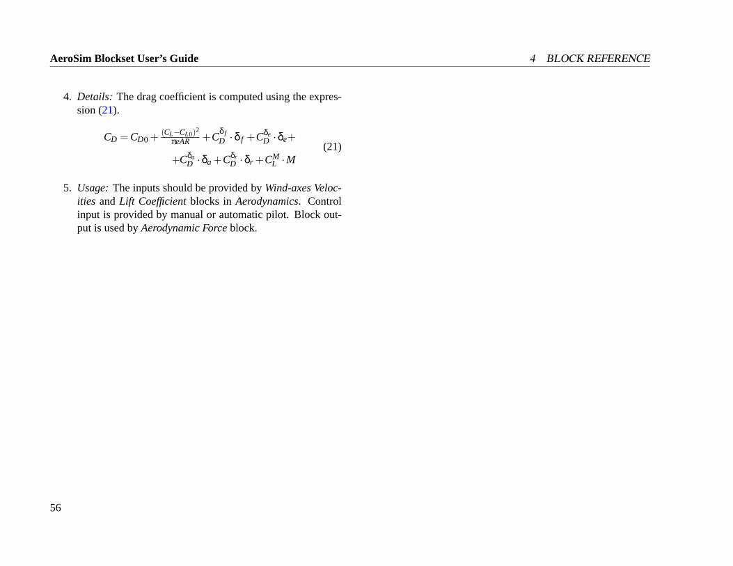
AeroSim Blockset User’s Guide 4 BLOCK REFERENCE
4. Details: The drag coefficient is computed using the expres-sion (21).
CD = CD0 + (CL−CL0)2
πeAR +Cδ fD ·δ f +Cδe
D ·δe+
+CδaD ·δa +Cδr
D ·δr +CML ·M
(21)
5. Usage:The inputs should be provided byWind-axes Veloc-ities andLift Coefficientblocks inAerodynamics. Controlinput is provided by manual or automatic pilot. Block out-put is used byAerodynamic Forceblock.
56
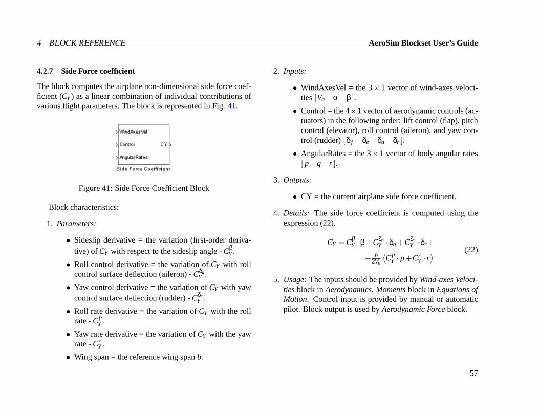
4 BLOCK REFERENCE AeroSim Blockset User’s Guide
4.2.7 Side Force coefficient
The block computes the airplane non-dimensional side force coef-ficient (CY) as a linear combination of individual contributions ofvarious flight parameters. The block is represented in Fig.41.
Figure 41: Side Force Coefficient Block
Block characteristics:
1. Parameters:
• Sideslip derivative = the variation (first-order deriva-tive) of CY with respect to the sideslip angle -Cβ
Y.
• Roll control derivative = the variation ofCY with rollcontrol surface deflection (aileron) -Cδa
Y .
• Yaw control derivative = the variation ofCY with yawcontrol surface deflection (rudder) -Cδr
Y .
• Roll rate derivative = the variation ofCY with the rollrate -Cp
Y.
• Yaw rate derivative = the variation ofCY with the yawrate -Cr
Y.
• Wing span = the reference wing spanb.
2. Inputs:
• WindAxesVel = the 3×1 vector of wind-axes veloci-ties[Va α β ].
• Control = the 4×1 vector of aerodynamic controls (ac-tuators) in the following order: lift control (flap), pitchcontrol (elevator), roll control (aileron), and yaw con-trol (rudder)[δ f δe δa δr ].
• AngularRates = the 3×1 vector of body angular rates[ p q r].
3. Outputs:
• CY = the current airplane side force coefficient.
4. Details: The side force coefficient is computed using theexpression (22).
CY = CβY ·β+Cδa
Y ·δa +CδrY ·δr+
+ b2Va
(Cp
Y · p+CrY · r) (22)
5. Usage:The inputs should be provided byWind-axes Veloci-tiesblock in Aerodynamics, Momentsblock in Equations ofMotion. Control input is provided by manual or automaticpilot. Block output is used byAerodynamic Forceblock.
57
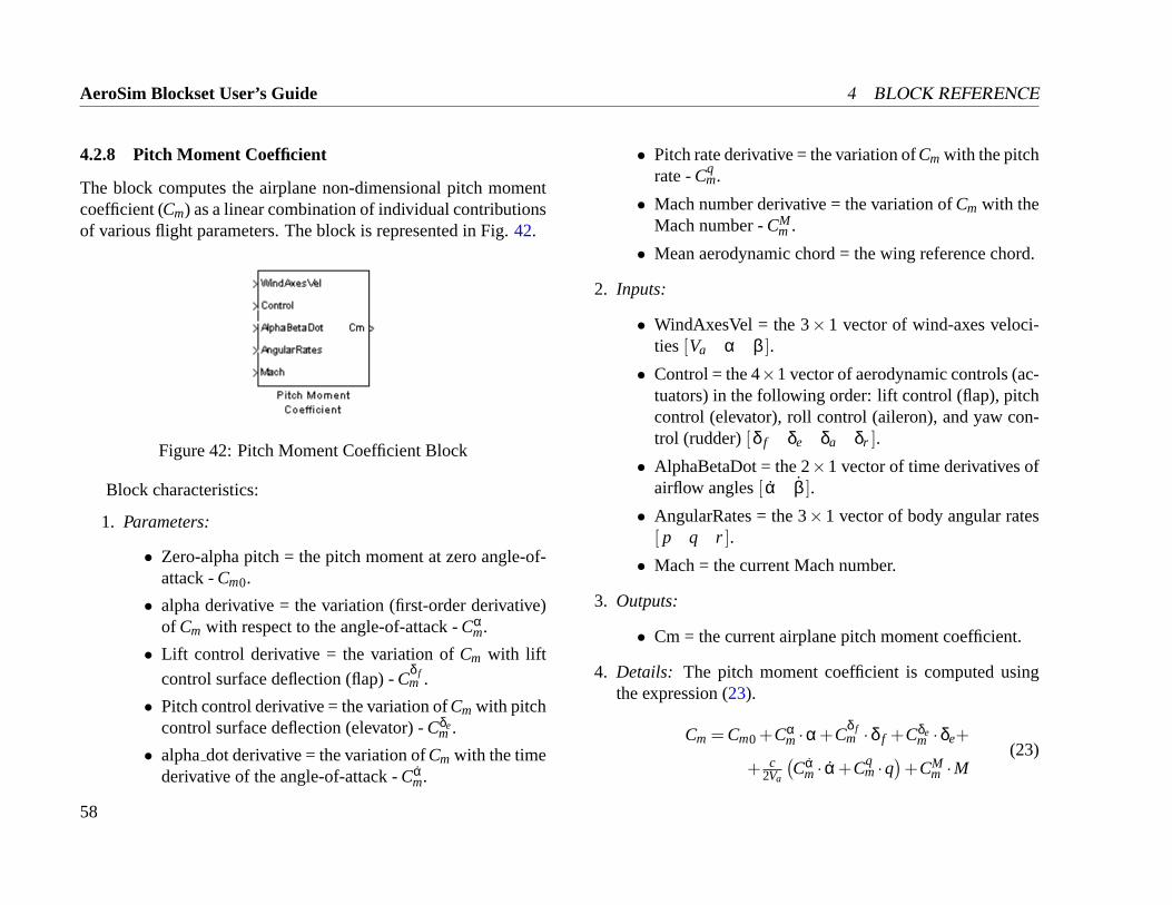
AeroSim Blockset User’s Guide 4 BLOCK REFERENCE
4.2.8 Pitch Moment Coefficient
The block computes the airplane non-dimensional pitch momentcoefficient (Cm) as a linear combination of individual contributionsof various flight parameters. The block is represented in Fig.42.
Figure 42: Pitch Moment Coefficient Block
Block characteristics:
1. Parameters:
• Zero-alpha pitch = the pitch moment at zero angle-of-attack -Cm0.
• alpha derivative = the variation (first-order derivative)of Cm with respect to the angle-of-attack -Cα
m.
• Lift control derivative = the variation ofCm with lift
control surface deflection (flap) -Cδ fm .
• Pitch control derivative = the variation ofCm with pitchcontrol surface deflection (elevator) -Cδe
m .
• alphadot derivative = the variation ofCm with the timederivative of the angle-of-attack -Cα
m.
• Pitch rate derivative = the variation ofCm with the pitchrate -Cq
m.
• Mach number derivative = the variation ofCm with theMach number -CM
m .
• Mean aerodynamic chord = the wing reference chord.
2. Inputs:
• WindAxesVel = the 3×1 vector of wind-axes veloci-ties[Va α β ].
• Control = the 4×1 vector of aerodynamic controls (ac-tuators) in the following order: lift control (flap), pitchcontrol (elevator), roll control (aileron), and yaw con-trol (rudder)[δ f δe δa δr ].
• AlphaBetaDot = the 2×1 vector of time derivatives ofairflow angles[ α β ].
• AngularRates = the 3×1 vector of body angular rates[ p q r].
• Mach = the current Mach number.
3. Outputs:
• Cm = the current airplane pitch moment coefficient.
4. Details: The pitch moment coefficient is computed usingthe expression (23).
Cm = Cm0 +Cαm ·α+C
δ fm ·δ f +Cδe
m ·δe+
+ c2Va
(Cα
m · α+Cqm ·q
)+CM
m ·M(23)
58
4 BLOCK REFERENCE AeroSim Blockset User’s Guide
5. Usage:The inputs should be provided byWind-axes Veloci-tiesblock in Aerodynamics, Momentsblock in Equations ofMotion. Control input is provided by manual or automaticpilot. Block output is used byAerodynamic Forceblock.
59
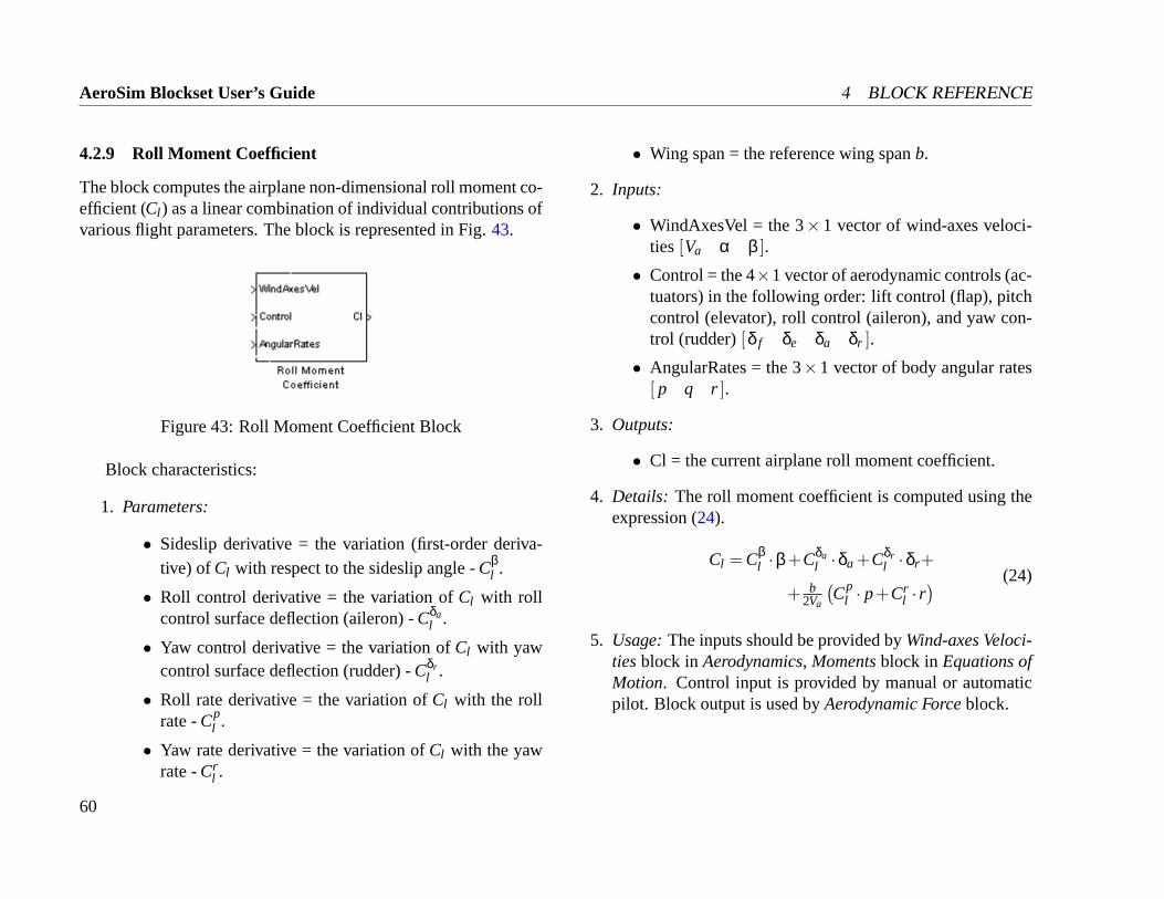
AeroSim Blockset User’s Guide 4 BLOCK REFERENCE
4.2.9 Roll Moment Coefficient
The block computes the airplane non-dimensional roll moment co-efficient (Cl ) as a linear combination of individual contributions ofvarious flight parameters. The block is represented in Fig.43.
Figure 43: Roll Moment Coefficient Block
Block characteristics:
1. Parameters:
• Sideslip derivative = the variation (first-order deriva-tive) of Cl with respect to the sideslip angle -Cβ
l .
• Roll control derivative = the variation ofCl with rollcontrol surface deflection (aileron) -Cδa
l .
• Yaw control derivative = the variation ofCl with yawcontrol surface deflection (rudder) -Cδr
l .
• Roll rate derivative = the variation ofCl with the rollrate -Cp
l .
• Yaw rate derivative = the variation ofCl with the yawrate -Cr
l .
• Wing span = the reference wing spanb.
2. Inputs:
• WindAxesVel = the 3×1 vector of wind-axes veloci-ties[Va α β ].
• Control = the 4×1 vector of aerodynamic controls (ac-tuators) in the following order: lift control (flap), pitchcontrol (elevator), roll control (aileron), and yaw con-trol (rudder)[δ f δe δa δr ].
• AngularRates = the 3×1 vector of body angular rates[ p q r].
3. Outputs:
• Cl = the current airplane roll moment coefficient.
4. Details: The roll moment coefficient is computed using theexpression (24).
Cl = Cβl ·β+Cδa
l ·δa +Cδrl ·δr+
+ b2Va
(Cp
l · p+Crl · r) (24)
5. Usage:The inputs should be provided byWind-axes Veloci-tiesblock in Aerodynamics, Momentsblock in Equations ofMotion. Control input is provided by manual or automaticpilot. Block output is used byAerodynamic Forceblock.
60
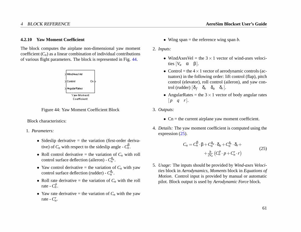
4 BLOCK REFERENCE AeroSim Blockset User’s Guide
4.2.10 Yaw Moment Coefficient
The block computes the airplane non-dimensional yaw momentcoefficient (Cn) as a linear combination of individual contributionsof various flight parameters. The block is represented in Fig.44.
Figure 44: Yaw Moment Coefficient Block
Block characteristics:
1. Parameters:
• Sideslip derivative = the variation (first-order deriva-tive) of Cn with respect to the sideslip angle -Cβ
n .
• Roll control derivative = the variation ofCn with rollcontrol surface deflection (aileron) -Cδa
n .
• Yaw control derivative = the variation ofCn with yawcontrol surface deflection (rudder) -Cδr
n .
• Roll rate derivative = the variation ofCn with the rollrate -Cp
n .
• Yaw rate derivative = the variation ofCn with the yawrate -Cr
n.
• Wing span = the reference wing spanb.
2. Inputs:
• WindAxesVel = the 3×1 vector of wind-axes veloci-ties[Va α β ].
• Control = the 4×1 vector of aerodynamic controls (ac-tuators) in the following order: lift control (flap), pitchcontrol (elevator), roll control (aileron), and yaw con-trol (rudder)[δ f δe δa δr ].
• AngularRates = the 3×1 vector of body angular rates[ p q r].
3. Outputs:
• Cn = the current airplane yaw moment coefficient.
4. Details: The yaw moment coefficient is computed using theexpression (25).
Cn = Cβn ·β+Cδa
n ·δa +Cδrn ·δr+
+ b2Va
(Cp
n · p+Crn · r) (25)
5. Usage:The inputs should be provided byWind-axes Veloci-tiesblock in Aerodynamics, Momentsblock in Equations ofMotion. Control input is provided by manual or automaticpilot. Block output is used byAerodynamic Forceblock.
61
AeroSim Blockset User’s Guide 4 BLOCK REFERENCE
4.3 Atmosphere
TheAtmosphere library folder includes blocks to estimate the airparameters and the wind effects.
62
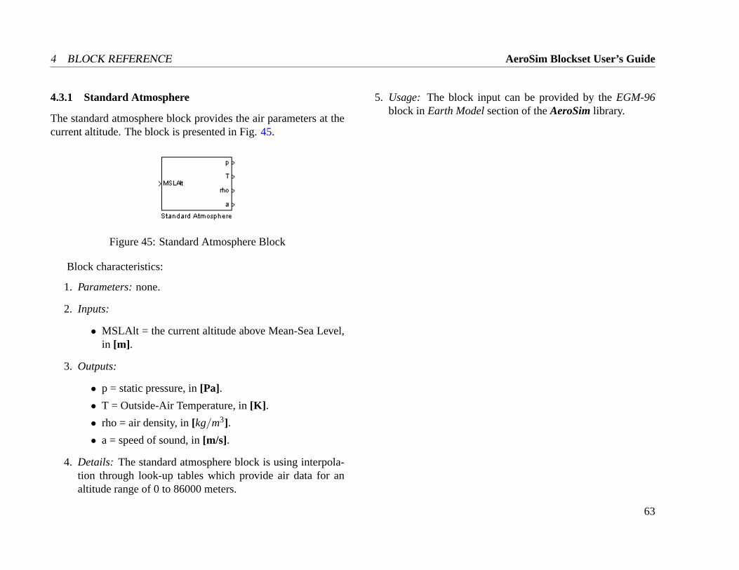
4 BLOCK REFERENCE AeroSim Blockset User’s Guide
4.3.1 Standard Atmosphere
The standard atmosphere block provides the air parameters at thecurrent altitude. The block is presented in Fig.45.
Figure 45: Standard Atmosphere Block
Block characteristics:
1. Parameters:none.
2. Inputs:
• MSLAlt = the current altitude above Mean-Sea Level,in [m] .
3. Outputs:
• p = static pressure, in[Pa].
• T = Outside-Air Temperature, in[K] .
• rho = air density, in[kg/m3].
• a = speed of sound, in[m/s].
4. Details: The standard atmosphere block is using interpola-tion through look-up tables which provide air data for analtitude range of 0 to 86000 meters.
5. Usage: The block input can be provided by theEGM-96block inEarth Modelsection of theAeroSimlibrary.
63
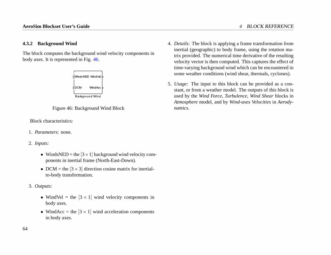
AeroSim Blockset User’s Guide 4 BLOCK REFERENCE
4.3.2 Background Wind
The block computes the background wind velocity components inbody axes. It is represented in Fig.46.
Figure 46: Background Wind Block
Block characteristics:
1. Parameters:none.
2. Inputs:
• WindsNED = the[3×1] background wind velocity com-ponents in inertial frame (North-East-Down).
• DCM = the[3×3] direction cosine matrix for inertial-to-body transformation.
3. Outputs:
• WindVel = the [3× 1] wind velocity components inbody axes.
• WindAcc = the[3×1] wind acceleration componentsin body axes.
4. Details: The block is applying a frame transformation frominertial (geographic) to body frame, using the rotation ma-trix provided. The numerical time derivative of the resultingvelocity vector is then computed. This captures the effect oftime-varying background wind which can be encountered insome weather conditions (wind shear, thermals, cyclones).
5. Usage: The input to this block can be provided as a con-stant, or from a weather model. The outputs of this block isused by theWind Force, Turbulence, Wind Shearblocks inAtmospheremodel, and byWind-axes Velocitiesin Aerody-namics.
64
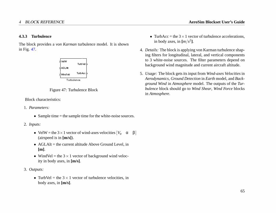
4 BLOCK REFERENCE AeroSim Blockset User’s Guide
4.3.3 Turbulence
The block provides avon Karmanturbulence model. It is shownin Fig. 47.
Figure 47: Turbulence Block
Block characteristics:
1. Parameters:
• Sample time = the sample time for the white-noise sources.
2. Inputs:
• VelW = the 3×1 vector of wind-axes velocities[Va α β ](airspeed is in[m/s]).
• AGLAlt = the current altitude Above Ground Level, in[m] .
• WindVel = the 3×1 vector of background wind veloc-ity in body axes, in[m/s].
3. Outputs:
• TurbVel = the 3×1 vector of turbulence velocities, inbody axes, in[m/s].
• TurbAcc = the 3×1 vector of turbulence accelerations,in body axes, in[m/s2].
4. Details: The block is applying von Karman turbulence shap-ing filters for longitudinal, lateral, and vertical componentsto 3 white-noise sources. The filter parameters depend onbackground wind magnitude and current aircraft altitude.
5. Usage:The block gets its input fromWind-axes VelocitiesinAerodynamics, Ground Detectionin Earthmodel, andBack-ground Windin Atmospheremodel. The outputs of theTur-bulenceblock should go toWind Shear, Wind Forceblocksin Atmosphere.
65
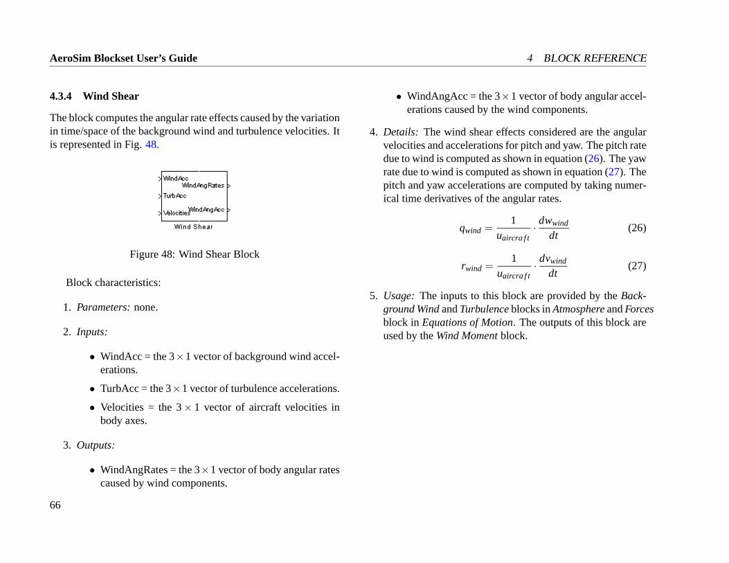
AeroSim Blockset User’s Guide 4 BLOCK REFERENCE
4.3.4 Wind Shear
The block computes the angular rate effects caused by the variationin time/space of the background wind and turbulence velocities. Itis represented in Fig.48.
Figure 48: Wind Shear Block
Block characteristics:
1. Parameters:none.
2. Inputs:
• WindAcc = the 3×1 vector of background wind accel-erations.
• TurbAcc = the 3×1 vector of turbulence accelerations.
• Velocities = the 3× 1 vector of aircraft velocities inbody axes.
3. Outputs:
• WindAngRates = the 3×1 vector of body angular ratescaused by wind components.
• WindAngAcc = the 3×1 vector of body angular accel-erations caused by the wind components.
4. Details: The wind shear effects considered are the angularvelocities and accelerations for pitch and yaw. The pitch ratedue to wind is computed as shown in equation (26). The yawrate due to wind is computed as shown in equation (27). Thepitch and yaw accelerations are computed by taking numer-ical time derivatives of the angular rates.
qwind =1
uaircra f t· dwwind
dt(26)
rwind =1
uaircra f t· dvwind
dt(27)
5. Usage: The inputs to this block are provided by theBack-ground WindandTurbulenceblocks inAtmosphereandForcesblock in Equations of Motion. The outputs of this block areused by theWind Momentblock.
66
4 BLOCK REFERENCE AeroSim Blockset User’s Guide
4.4 Complete Aircraft
The Complete Aircraft folder provides complete aircraft mod-els built usingAeroSim library blocks. These models are con-figurable via parameter files which should be in ”mat” format. Atemplate and sample Matlab scripts that can be used to generatethis type of aircraft parameter files can be found in thesamplesdirectory, under the mainAeroSim library directory.
67
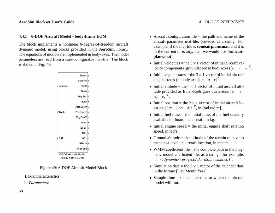
AeroSim Blockset User’s Guide 4 BLOCK REFERENCE
4.4.1 6-DOF Aircraft Model - body-frame EOM
The block implements a nonlinear 6-degree-of-freedom aircraftdynamic model, using blocks provided in theAeroSim library.The equations of motion are implemented in body-axes. The modelparameters are read from a user-configurable mat-file. The blockis shown in Fig.49.
Figure 49: 6-DOF Aircraft Model Block
Block characteristics:
1. Parameters:
• Aircraft configuration file = the path and name of theaircraft parameter mat-file, provided as a string. Forexample, if the mat-file issomeairplane.mat, and it isin the current directory, then we would use’someair-plane.mat’.
• Initial velocities = the 3×1 vector of initial aircraft ve-locity components (groundspeed in body axes)[u v w]T .
• Initial angular rates = the 3×1 vector of initial aircraftangular rates (in body axes)[ p q r]T .
• Initial attitude = the 4×1 vector of initial aircraft atti-tude provided as Euler-Rodrigues quaterions[e0 ex
ey ez]T .
• Initial position = the 3×1 vector of initial aircraft lo-cation[Lat Lon Alt]T , in [rad rad m].
• Initial fuel mass = the initial mass of the fuel quantityavailable on-board the aircraft, in kg.
• Initial engine speed = the initial engine shaft rotationspeed, in rad/s.
• Ground altitude = the altitude of the terrain relative tomean-sea-level, at aircraft location, in meters.
• WMM coefficient file = the complete path to the mag-netic model coefficient file, as a string - for example,′c : \udynamics\pro jects\AeroSim\wmm.co f′.
• Simulation date = the 3×1 vector of the calendar datein the format [Day Month Year].
• Sample time = the sample time at which the aircraftmodel will run.
68
4 BLOCK REFERENCE AeroSim Blockset User’s Guide
2. Inputs:
• Controls = the 7×1 vector of aircraft controls[ f lapelevator aileron rudder throttle mixture ignition]T
in [rad rad rad rad frac ratio bool].
• Winds = the 3×1 vector of background wind veloci-ties, in navigation frame[WN WE WD ]T , in m/s.
• RST = the integrator reset flag (can take values of 0 or1, all integrators reset on rising-edge).
3. Outputs:
• States = the 15×1 vector of aircraft states[u v w pq r e0 ex ey ez Lat Lon Alt mf uel Ωeng]
T .
• Sensors = the 18×1 vector of sensor data[Lat Lon AltVN VE VD ax ay az p q r pstat pdyn
OAT Hx Hy Hz]T .
• VelW = the 3× 1 vector of aircraft velocity in windaxes[Va β α ]T in [m/s rad rad].
• Mach = the current aircraft Mach number.
• Angular Acc = the 3×1 vector of body angular accel-erations[ p q r ]T .
• Euler = the 3×1 vector of the attitude of the aircraftgiven in Euler angles[φ θ ψ ]T , in radians.
• AeroCoeff = the 6× 1 vector of aerodynamic coeffi-cients[CD CY CL Cl Cm Cn ]T , in rad−1.
• PropCoeff = the 3×1 vector of propeller coefficients[J CT CP ]T .
• EngCoeff = the 5×1 vector of engine coefficients[MAPmair mf uel BSFC P]T given in [kPa kg/s kg/s g/(W*hr)W].
• Mass = the current aircraft mass, in kg.
• ECEF = the 3× 1 vector of aircraft position in theEarth-centered, Earth-fixed frame[X Y Z]T .
• MSL = the aircraft altitude above mean-sea-level, inm.
• AGL = the aircraft altitude above ground, in m.
• REarth = the Earth equivalent radius, at current aircraftlocation, in m.
• AConGnd = the aircraft-on-the-ground flag (0 if air-craft above ground, 1 if aircraft is on the ground).
4. Details: Most of the AeroSim blocks are used in this com-plete aircraft model. The blocks not included are the sensormodels, actuator models, and pilot interface blocks (joystickinput and graphical output).
The model reads the aircraft parameters at the start of sim-ulation from the specified mat-file. The mat-file is gen-erated by the user for a particular aircraft model, by cus-tomizing and running an aircraft configuration script (Mat-lab program). An aircraft configuration script template aswell as sample aircraft configuration scripts can be found intheSamplesdirectory under the AeroSim tree.
5. Usage: The complete aircraft model can be used for mod-eling and simulating the dynamics of a conventional aircraft
69

AeroSim Blockset User’s Guide 4 BLOCK REFERENCE
with single piston engine and fixed pitch propeller. Specificaircraft parameters are set from a user-generated configura-tion script. Control inputs can be provided from a joystickfor manual flight, or from an autopilot block for autonomousflight. Simulation output can be visualized using the FlightSimulator or FlightGear interface blocks.
70
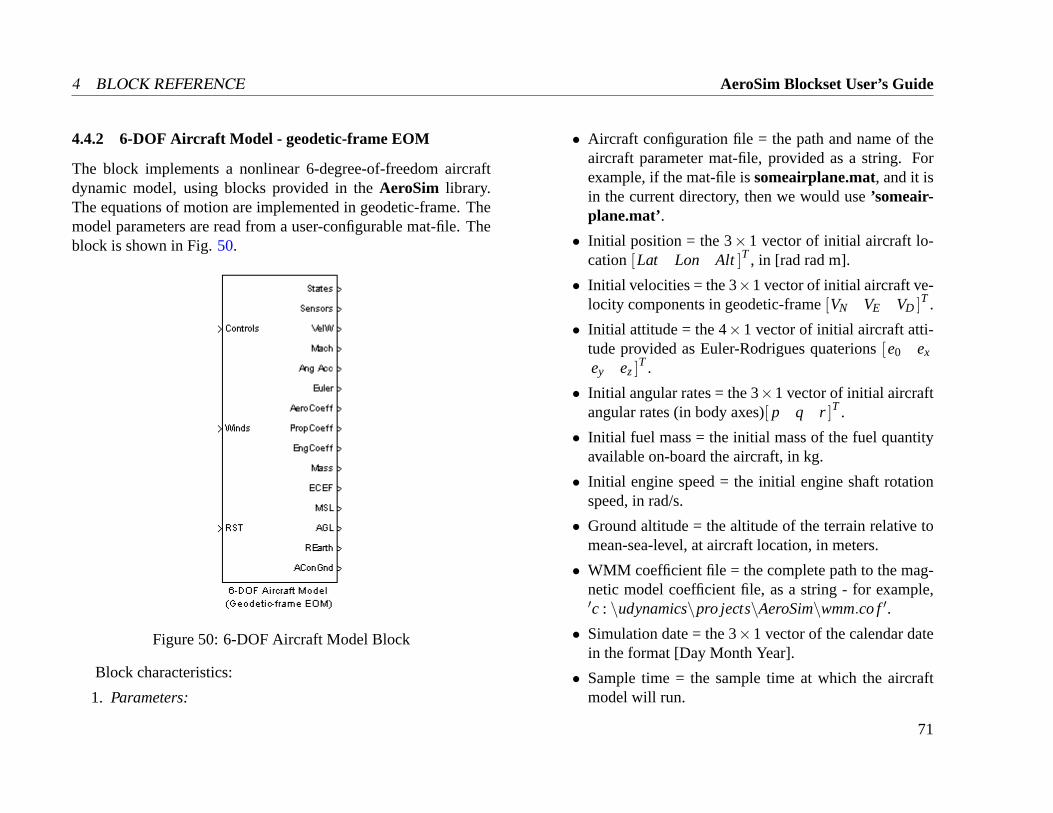
4 BLOCK REFERENCE AeroSim Blockset User’s Guide
4.4.2 6-DOF Aircraft Model - geodetic-frame EOM
The block implements a nonlinear 6-degree-of-freedom aircraftdynamic model, using blocks provided in theAeroSim library.The equations of motion are implemented in geodetic-frame. Themodel parameters are read from a user-configurable mat-file. Theblock is shown in Fig.50.
Figure 50: 6-DOF Aircraft Model Block
Block characteristics:
1. Parameters:
• Aircraft configuration file = the path and name of theaircraft parameter mat-file, provided as a string. Forexample, if the mat-file issomeairplane.mat, and it isin the current directory, then we would use’someair-plane.mat’.
• Initial position = the 3×1 vector of initial aircraft lo-cation[Lat Lon Alt]T , in [rad rad m].
• Initial velocities = the 3×1 vector of initial aircraft ve-locity components in geodetic-frame[VN VE VD ]T .
• Initial attitude = the 4×1 vector of initial aircraft atti-tude provided as Euler-Rodrigues quaterions[e0 ex
ey ez]T .
• Initial angular rates = the 3×1 vector of initial aircraftangular rates (in body axes)[ p q r]T .
• Initial fuel mass = the initial mass of the fuel quantityavailable on-board the aircraft, in kg.
• Initial engine speed = the initial engine shaft rotationspeed, in rad/s.
• Ground altitude = the altitude of the terrain relative tomean-sea-level, at aircraft location, in meters.
• WMM coefficient file = the complete path to the mag-netic model coefficient file, as a string - for example,′c : \udynamics\pro jects\AeroSim\wmm.co f′.
• Simulation date = the 3×1 vector of the calendar datein the format [Day Month Year].
• Sample time = the sample time at which the aircraftmodel will run.
71

AeroSim Blockset User’s Guide 4 BLOCK REFERENCE
2. Inputs:
• Controls = the 7×1 vector of aircraft controls[ f lapelevator aileron rudder throttle mixture ignition]T
in [rad rad rad rad frac ratio bool].
• Winds = the 3×1 vector of background wind veloci-ties, in navigation frame[WN WE WD ]T , in m/s.
• RST = the integrator reset flag (can take values of 0 or1, all integrators reset on rising-edge).
3. Outputs:
• States = the 15×1 vector of aircraft states[VN VE VD pq r e0 ex ey ez Lat Lon Alt mf uel Ωeng]
T .
• Sensors = the 18×1 vector of sensor data[Lat Lon AltVN VE VD ax ay az p q r pstat pdyn
OAT Hx Hy Hz]T .
• VelW = the 3× 1 vector of aircraft velocity in windaxes[Va β α ]T in [m/s rad rad].
• Mach = the current aircraft Mach number.
• Angular Acc = the 3×1 vector of body angular accel-erations[ p q r ]T .
• Euler = the 3×1 vector of the attitude of the aircraftgiven in Euler angles[φ θ ψ ]T , in radians.
• AeroCoeff = the 6× 1 vector of aerodynamic coeffi-cients[CD CY CL Cl Cm Cn ]T , in rad−1.
• PropCoeff = the 3×1 vector of propeller coefficients[J CT CP ]T .
• EngCoeff = the 5×1 vector of engine coefficients[MAPmair mf uel BSFC P]T given in [kPa kg/s kg/s g/(W*hr)W].
• Mass = the current aircraft mass, in kg.
• ECEF = the 3× 1 vector of aircraft position in theEarth-centered, Earth-fixed frame[X Y Z]T .
• MSL = the aircraft altitude above mean-sea-level, inm.
• AGL = the aircraft altitude above ground, in m.
• REarth = the Earth equivalent radius, at current aircraftlocation, in m.
• AConGnd = the aircraft-on-the-ground flag (0 if air-craft above ground, 1 if aircraft is on the ground).
4. Details: Most of the AeroSim blocks are used in this com-plete aircraft model. The blocks not included are the sensormodels, actuator models, and pilot interface blocks (joystickinput and graphical output).
The model reads the aircraft parameters at the start of sim-ulation from the specified mat-file. The mat-file is gen-erated by the user for a particular aircraft model, by cus-tomizing and running an aircraft configuration script (Mat-lab program). An aircraft configuration script template aswell as sample aircraft configuration scripts can be found intheSamplesdirectory under the AeroSim tree.
5. Usage: The complete aircraft model can be used for mod-eling and simulating the dynamics of a conventional aircraft
72
4 BLOCK REFERENCE AeroSim Blockset User’s Guide
with single piston engine and fixed pitch propeller. Specificaircraft parameters are set from a user-generated configura-tion script. Control inputs can be provided from a joystickfor manual flight, or from an autopilot block for autonomousflight. Simulation output can be visualized using the FlightSimulator or FlightGear interface blocks.
73
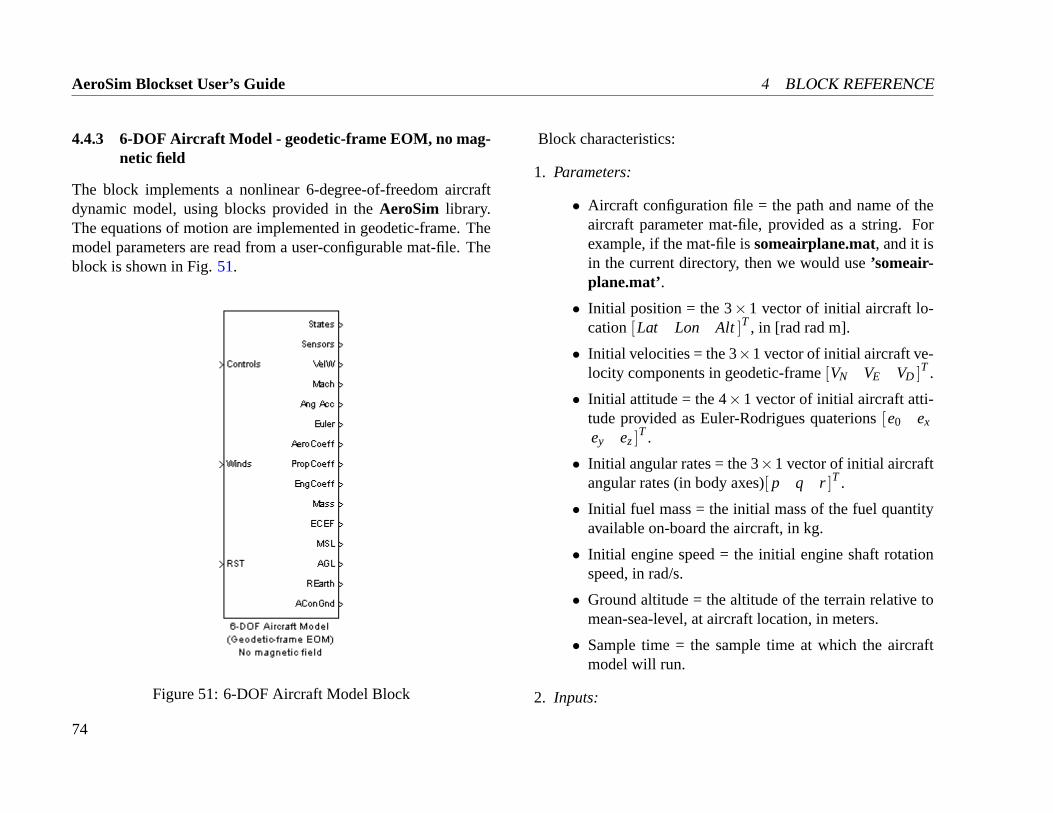
AeroSim Blockset User’s Guide 4 BLOCK REFERENCE
4.4.3 6-DOF Aircraft Model - geodetic-frame EOM, no mag-netic field
The block implements a nonlinear 6-degree-of-freedom aircraftdynamic model, using blocks provided in theAeroSim library.The equations of motion are implemented in geodetic-frame. Themodel parameters are read from a user-configurable mat-file. Theblock is shown in Fig.51.
Figure 51: 6-DOF Aircraft Model Block
Block characteristics:
1. Parameters:
• Aircraft configuration file = the path and name of theaircraft parameter mat-file, provided as a string. Forexample, if the mat-file issomeairplane.mat, and it isin the current directory, then we would use’someair-plane.mat’.
• Initial position = the 3×1 vector of initial aircraft lo-cation[Lat Lon Alt]T , in [rad rad m].
• Initial velocities = the 3×1 vector of initial aircraft ve-locity components in geodetic-frame[VN VE VD ]T .
• Initial attitude = the 4×1 vector of initial aircraft atti-tude provided as Euler-Rodrigues quaterions[e0 ex
ey ez]T .
• Initial angular rates = the 3×1 vector of initial aircraftangular rates (in body axes)[ p q r]T .
• Initial fuel mass = the initial mass of the fuel quantityavailable on-board the aircraft, in kg.
• Initial engine speed = the initial engine shaft rotationspeed, in rad/s.
• Ground altitude = the altitude of the terrain relative tomean-sea-level, at aircraft location, in meters.
• Sample time = the sample time at which the aircraftmodel will run.
2. Inputs:
74
4 BLOCK REFERENCE AeroSim Blockset User’s Guide
• Controls = the 7×1 vector of aircraft controls[ f lapelevator aileron rudder throttle mixture ignition]T
in [rad rad rad rad frac ratio bool].
• Winds = the 3×1 vector of background wind veloci-ties, in navigation frame[WN WE WD ]T , in m/s.
• RST = the integrator reset flag (can take values of 0 or1, all integrators reset on rising-edge).
3. Outputs:
• States = the 15×1 vector of aircraft states[VN VE VD pq r e0 ex ey ez Lat Lon Alt mf uel Ωeng]
T .
• Sensors = the 15×1 vector of sensor data[Lat Lon AltVN VE VD ax ay az p q r pstat pdyn OAT]T .
• VelW = the 3× 1 vector of aircraft velocity in windaxes[Va β α ]T in [m/s rad rad].
• Mach = the current aircraft Mach number.
• Angular Acc = the 3×1 vector of body angular accel-erations[ p q r ]T .
• Euler = the 3×1 vector of the attitude of the aircraftgiven in Euler angles[φ θ ψ ]T , in radians.
• AeroCoeff = the 6× 1 vector of aerodynamic coeffi-cients[CD CY CL Cl Cm Cn ]T , in rad−1.
• PropCoeff = the 3×1 vector of propeller coefficients[J CT CP ]T .
• EngCoeff = the 5×1 vector of engine coefficients[MAPmair mf uel BSFC P]T given in [kPa kg/s kg/s g/(W*hr)W].
• Mass = the current aircraft mass, in kg.
• ECEF = the 3× 1 vector of aircraft position in theEarth-centered, Earth-fixed frame[X Y Z]T .
• MSL = the aircraft altitude above mean-sea-level, inm.
• AGL = the aircraft altitude above ground, in m.
• REarth = the Earth equivalent radius, at current aircraftlocation, in m.
• AConGnd = the aircraft-on-the-ground flag (0 if air-craft above ground, 1 if aircraft is on the ground).
4. Details: Most of the AeroSim blocks are used in this com-plete aircraft model. The blocks not included are the sensormodels, actuator models, and pilot interface blocks (joystickinput and graphical output).
The model reads the aircraft parameters at the start of sim-ulation from the specified mat-file. The mat-file is gen-erated by the user for a particular aircraft model, by cus-tomizing and running an aircraft configuration script (Mat-lab program). An aircraft configuration script template aswell as sample aircraft configuration scripts can be found intheSamplesdirectory under the AeroSim tree.
5. Usage: The complete aircraft model can be used for mod-eling and simulating the dynamics of a conventional aircraftwith single piston engine and fixed pitch propeller. Specificaircraft parameters are set from a user-generated configura-tion script. Control inputs can be provided from a joystickfor manual flight, or from an autopilot block for autonomous
75
AeroSim Blockset User’s Guide 4 BLOCK REFERENCE
flight. Simulation output can be visualized using the FlightSimulator or FlightGear interface blocks.
76
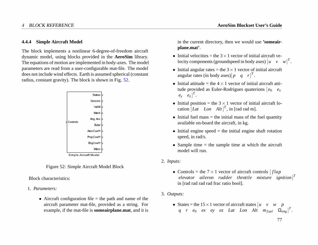
4 BLOCK REFERENCE AeroSim Blockset User’s Guide
4.4.4 Simple Aircraft Model
The block implements a nonlinear 6-degree-of-freedom aircraftdynamic model, using blocks provided in theAeroSim library.The equations of motion are implemented in body-axes. The modelparameters are read from a user-configurable mat-file. The modeldoes not include wind effects. Earth is assumed spherical (constantradius, constant gravity). The block is shown in Fig.52.
Figure 52: Simple Aircraft Model Block
Block characteristics:
1. Parameters:
• Aircraft configuration file = the path and name of theaircraft parameter mat-file, provided as a string. Forexample, if the mat-file issomeairplane.mat, and it is
in the current directory, then we would use’someair-plane.mat’.
• Initial velocities = the 3×1 vector of initial aircraft ve-locity components (groundspeed in body axes)[u v w]T .
• Initial angular rates = the 3×1 vector of initial aircraftangular rates (in body axes)[ p q r]T .
• Initial attitude = the 4×1 vector of initial aircraft atti-tude provided as Euler-Rodrigues quaterions[e0 ex
ey ez]T .
• Initial position = the 3×1 vector of initial aircraft lo-cation[Lat Lon Alt]T , in [rad rad m].
• Initial fuel mass = the initial mass of the fuel quantityavailable on-board the aircraft, in kg.
• Initial engine speed = the initial engine shaft rotationspeed, in rad/s.
• Sample time = the sample time at which the aircraftmodel will run.
2. Inputs:
• Controls = the 7×1 vector of aircraft controls[ f lapelevator aileron rudder throttle mixture ignition]T
in [rad rad rad rad frac ratio bool].
3. Outputs:
• States = the 15×1 vector of aircraft states[u v w pq r e0 ex ey ez Lat Lon Alt mf uel Ωeng]
T .
77
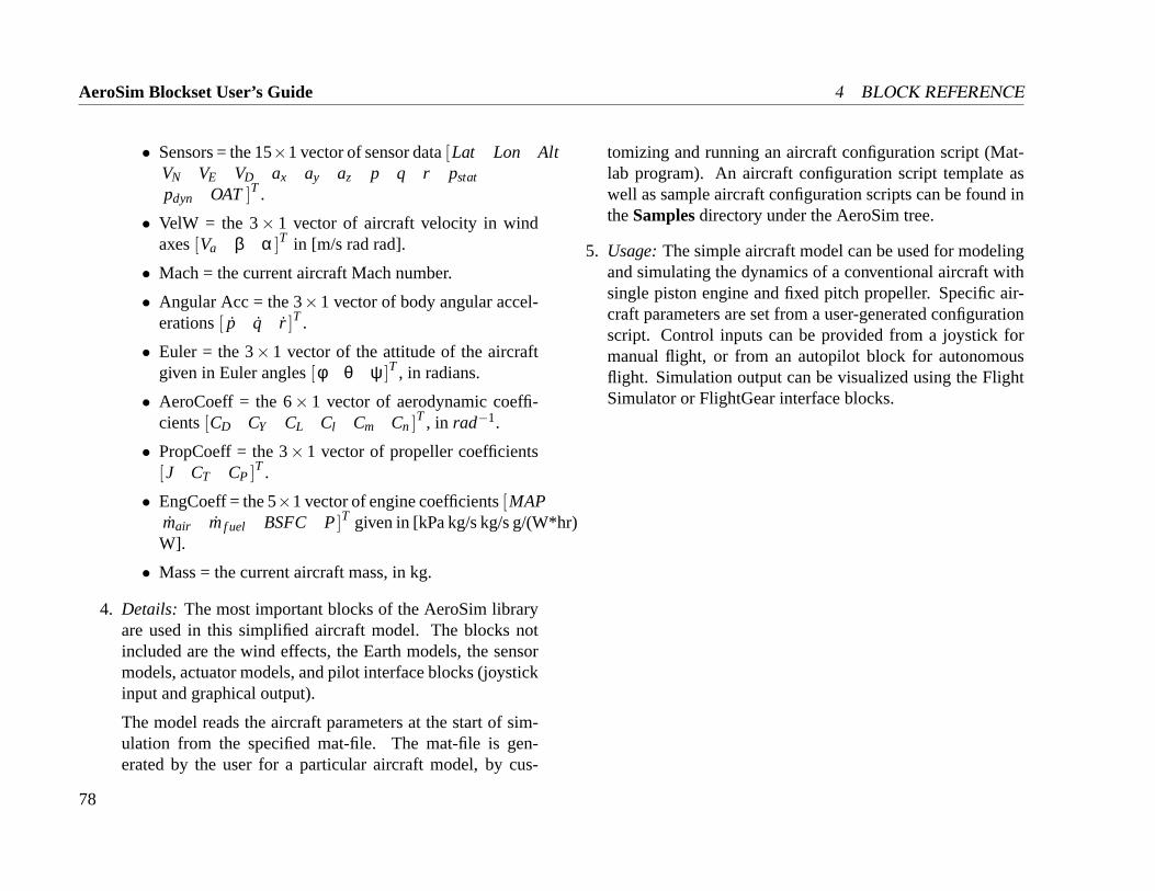
AeroSim Blockset User’s Guide 4 BLOCK REFERENCE
• Sensors = the 15×1 vector of sensor data[Lat Lon AltVN VE VD ax ay az p q r pstat
pdyn OAT]T .
• VelW = the 3× 1 vector of aircraft velocity in windaxes[Va β α ]T in [m/s rad rad].
• Mach = the current aircraft Mach number.
• Angular Acc = the 3×1 vector of body angular accel-erations[ p q r ]T .
• Euler = the 3×1 vector of the attitude of the aircraftgiven in Euler angles[φ θ ψ ]T , in radians.
• AeroCoeff = the 6× 1 vector of aerodynamic coeffi-cients[CD CY CL Cl Cm Cn ]T , in rad−1.
• PropCoeff = the 3×1 vector of propeller coefficients[J CT CP ]T .
• EngCoeff = the 5×1 vector of engine coefficients[MAPmair mf uel BSFC P]T given in [kPa kg/s kg/s g/(W*hr)W].
• Mass = the current aircraft mass, in kg.
4. Details: The most important blocks of the AeroSim libraryare used in this simplified aircraft model. The blocks notincluded are the wind effects, the Earth models, the sensormodels, actuator models, and pilot interface blocks (joystickinput and graphical output).
The model reads the aircraft parameters at the start of sim-ulation from the specified mat-file. The mat-file is gen-erated by the user for a particular aircraft model, by cus-
tomizing and running an aircraft configuration script (Mat-lab program). An aircraft configuration script template aswell as sample aircraft configuration scripts can be found intheSamplesdirectory under the AeroSim tree.
5. Usage:The simple aircraft model can be used for modelingand simulating the dynamics of a conventional aircraft withsingle piston engine and fixed pitch propeller. Specific air-craft parameters are set from a user-generated configurationscript. Control inputs can be provided from a joystick formanual flight, or from an autopilot block for autonomousflight. Simulation output can be visualized using the FlightSimulator or FlightGear interface blocks.
78
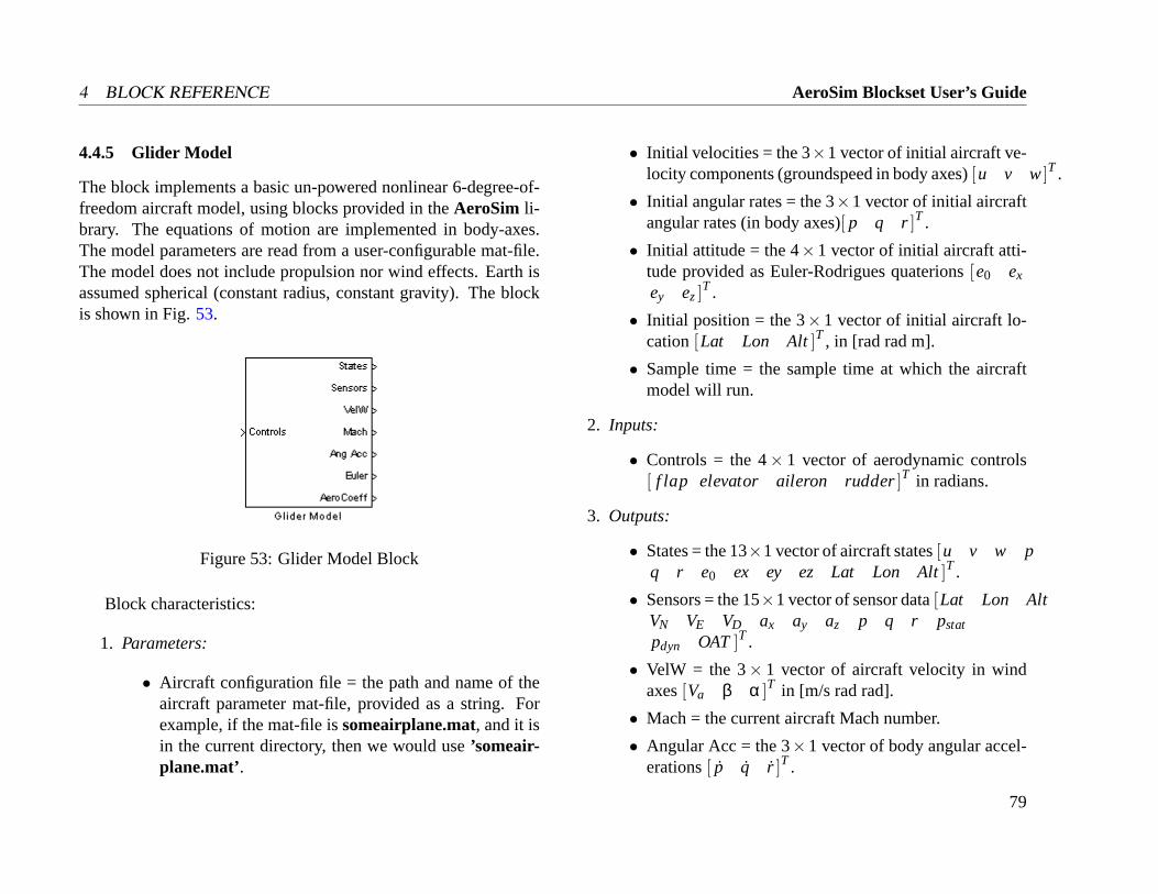
4 BLOCK REFERENCE AeroSim Blockset User’s Guide
4.4.5 Glider Model
The block implements a basic un-powered nonlinear 6-degree-of-freedom aircraft model, using blocks provided in theAeroSim li-brary. The equations of motion are implemented in body-axes.The model parameters are read from a user-configurable mat-file.The model does not include propulsion nor wind effects. Earth isassumed spherical (constant radius, constant gravity). The blockis shown in Fig.53.
Figure 53: Glider Model Block
Block characteristics:
1. Parameters:
• Aircraft configuration file = the path and name of theaircraft parameter mat-file, provided as a string. Forexample, if the mat-file issomeairplane.mat, and it isin the current directory, then we would use’someair-plane.mat’.
• Initial velocities = the 3×1 vector of initial aircraft ve-locity components (groundspeed in body axes)[u v w]T .
• Initial angular rates = the 3×1 vector of initial aircraftangular rates (in body axes)[ p q r]T .
• Initial attitude = the 4×1 vector of initial aircraft atti-tude provided as Euler-Rodrigues quaterions[e0 ex
ey ez]T .
• Initial position = the 3×1 vector of initial aircraft lo-cation[Lat Lon Alt]T , in [rad rad m].
• Sample time = the sample time at which the aircraftmodel will run.
2. Inputs:
• Controls = the 4× 1 vector of aerodynamic controls[ f lap elevator aileron rudder]T in radians.
3. Outputs:
• States = the 13×1 vector of aircraft states[u v w pq r e0 ex ey ez Lat Lon Alt]T .
• Sensors = the 15×1 vector of sensor data[Lat Lon AltVN VE VD ax ay az p q r pstat
pdyn OAT]T .
• VelW = the 3× 1 vector of aircraft velocity in windaxes[Va β α ]T in [m/s rad rad].
• Mach = the current aircraft Mach number.
• Angular Acc = the 3×1 vector of body angular accel-erations[ p q r ]T .
79
AeroSim Blockset User’s Guide 4 BLOCK REFERENCE
• Euler = the 3×1 vector of the attitude of the aircraftgiven in Euler angles[φ θ ψ ]T , in radians.
• AeroCoeff = the 6× 1 vector of aerodynamic coeffi-cients[CD CY CL Cl Cm Cn ]T , in rad−1.
4. Details: The most basic blocks of the AeroSim library areused in this simplified aircraft model. The blocks not in-cluded are the propulsion model, the wind effects, the Earthmodels, the sensor models, actuator models, and pilot inter-face blocks (joystick input and graphical output).
Since there is no propulsion nor fuel tank on-board, the air-craft inertia properties are assumed constant through-out theflight.
The model reads the aircraft parameters at the start of sim-ulation from the specified mat-file. The mat-file is gen-erated by the user for a particular aircraft model, by cus-tomizing and running an aircraft configuration script (Mat-lab program). An aircraft configuration script template aswell as sample aircraft configuration scripts can be found intheSamplesdirectory under the AeroSim tree.
5. Usage:The simple aircraft model can be used for modelingand simulating the dynamics of a conventional aircraft withsingle piston engine and fixed pitch propeller. Specific air-craft parameters are set from a user-generated configurationscript. Control inputs can be provided from a joystick formanual flight, or from an autopilot block for autonomousflight. Simulation output can be visualized using the FlightSimulator or FlightGear interface blocks.
80
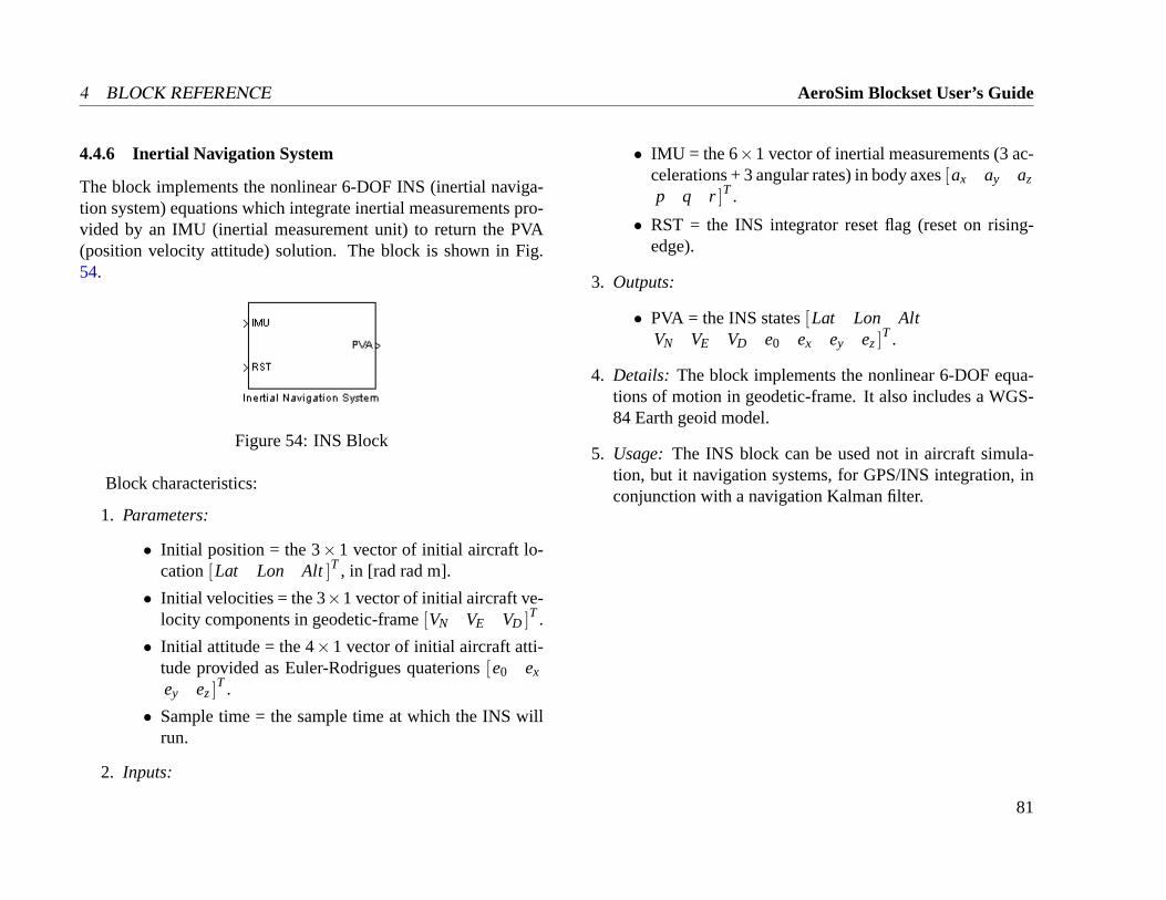
4 BLOCK REFERENCE AeroSim Blockset User’s Guide
4.4.6 Inertial Navigation System
The block implements the nonlinear 6-DOF INS (inertial naviga-tion system) equations which integrate inertial measurements pro-vided by an IMU (inertial measurement unit) to return the PVA(position velocity attitude) solution. The block is shown in Fig.54.
Figure 54: INS Block
Block characteristics:
1. Parameters:
• Initial position = the 3×1 vector of initial aircraft lo-cation[Lat Lon Alt]T , in [rad rad m].
• Initial velocities = the 3×1 vector of initial aircraft ve-locity components in geodetic-frame[VN VE VD ]T .
• Initial attitude = the 4×1 vector of initial aircraft atti-tude provided as Euler-Rodrigues quaterions[e0 ex
ey ez]T .
• Sample time = the sample time at which the INS willrun.
2. Inputs:
• IMU = the 6×1 vector of inertial measurements (3 ac-celerations + 3 angular rates) in body axes[ax ay az
p q r]T .
• RST = the INS integrator reset flag (reset on rising-edge).
3. Outputs:
• PVA = the INS states[Lat Lon AltVN VE VD e0 ex ey ez]
T .
4. Details: The block implements the nonlinear 6-DOF equa-tions of motion in geodetic-frame. It also includes a WGS-84 Earth geoid model.
5. Usage: The INS block can be used not in aircraft simula-tion, but it navigation systems, for GPS/INS integration, inconjunction with a navigation Kalman filter.
81

AeroSim Blockset User’s Guide 4 BLOCK REFERENCE
4.5 Earth
The Earth library folder includes blocks that model the Earth’sshape, gravity, and magnetic field.
82
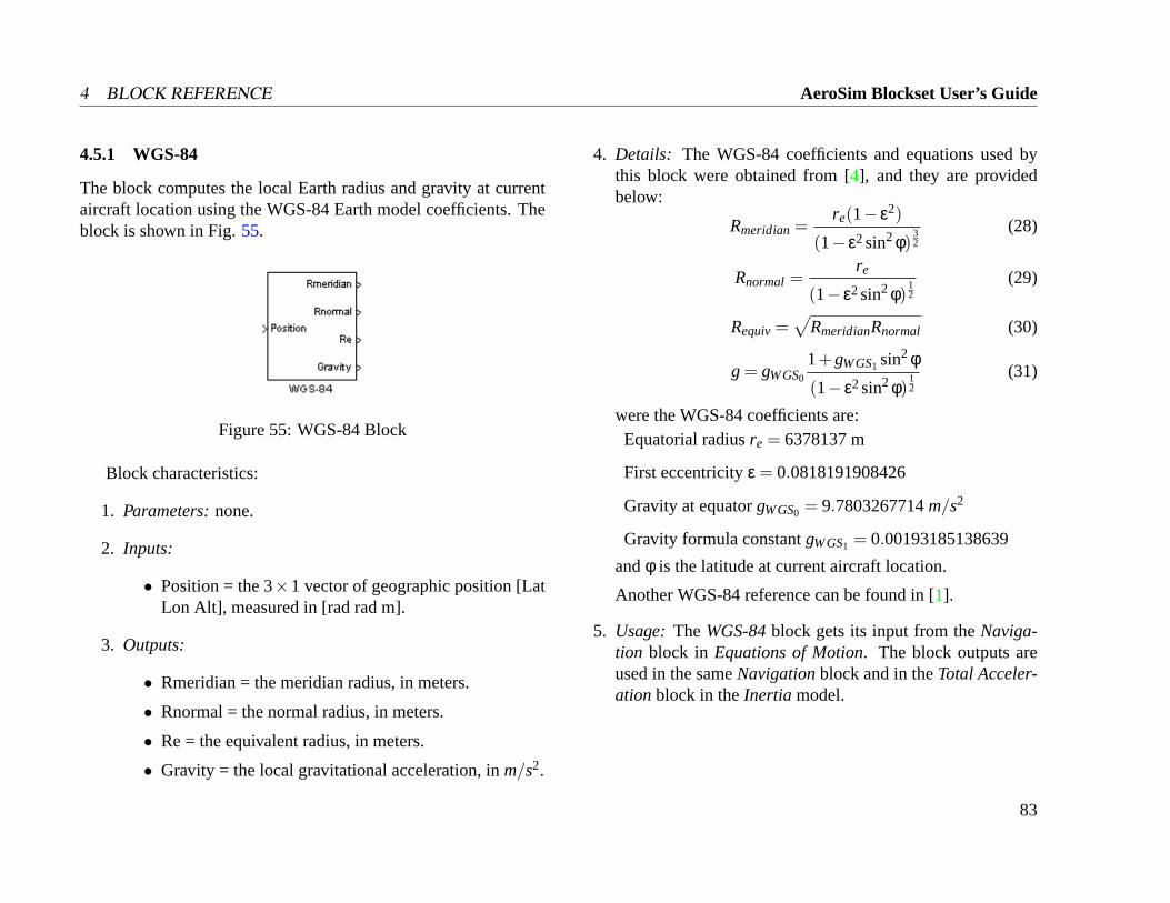
4 BLOCK REFERENCE AeroSim Blockset User’s Guide
4.5.1 WGS-84
The block computes the local Earth radius and gravity at currentaircraft location using the WGS-84 Earth model coefficients. Theblock is shown in Fig.55.
Figure 55: WGS-84 Block
Block characteristics:
1. Parameters:none.
2. Inputs:
• Position = the 3×1 vector of geographic position [LatLon Alt], measured in [rad rad m].
3. Outputs:
• Rmeridian = the meridian radius, in meters.
• Rnormal = the normal radius, in meters.
• Re = the equivalent radius, in meters.
• Gravity = the local gravitational acceleration, inm/s2.
4. Details: The WGS-84 coefficients and equations used bythis block were obtained from [4], and they are providedbelow:
Rmeridian=re(1− ε2)
(1− ε2sin2φ)32
(28)
Rnormal =re
(1− ε2sin2φ)12
(29)
Requiv=√
RmeridianRnormal (30)
g = gWGS0
1+gWGS1 sin2φ(1− ε2sin2φ)
12
(31)
were the WGS-84 coefficients are:Equatorial radiusre = 6378137 m
First eccentricityε = 0.0818191908426
Gravity at equatorgWGS0 = 9.7803267714m/s2
Gravity formula constantgWGS1 = 0.00193185138639
andφ is the latitude at current aircraft location.
Another WGS-84 reference can be found in [1].
5. Usage: TheWGS-84block gets its input from theNaviga-tion block in Equations of Motion. The block outputs areused in the sameNavigationblock and in theTotal Acceler-ationblock in theInertia model.
83
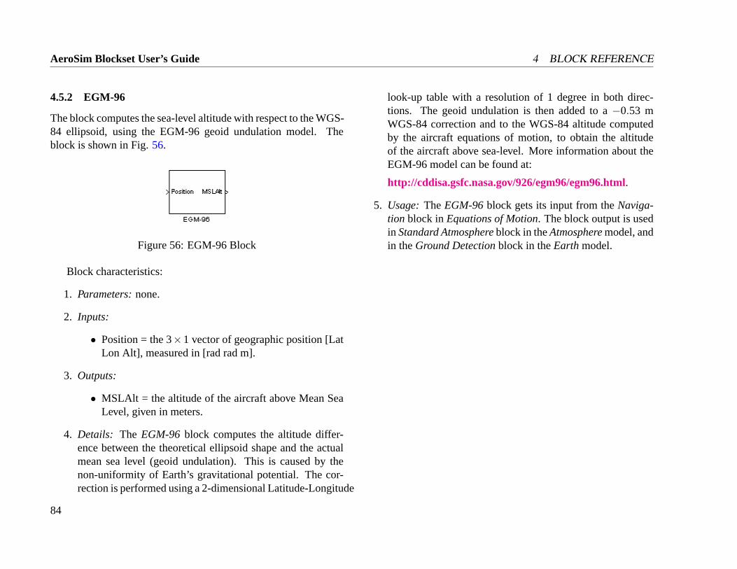
AeroSim Blockset User’s Guide 4 BLOCK REFERENCE
4.5.2 EGM-96
The block computes the sea-level altitude with respect to the WGS-84 ellipsoid, using the EGM-96 geoid undulation model. Theblock is shown in Fig.56.
Figure 56: EGM-96 Block
Block characteristics:
1. Parameters:none.
2. Inputs:
• Position = the 3×1 vector of geographic position [LatLon Alt], measured in [rad rad m].
3. Outputs:
• MSLAlt = the altitude of the aircraft above Mean SeaLevel, given in meters.
4. Details: The EGM-96 block computes the altitude differ-ence between the theoretical ellipsoid shape and the actualmean sea level (geoid undulation). This is caused by thenon-uniformity of Earth’s gravitational potential. The cor-rection is performed using a 2-dimensional Latitude-Longitude
look-up table with a resolution of 1 degree in both direc-tions. The geoid undulation is then added to a−0.53 mWGS-84 correction and to the WGS-84 altitude computedby the aircraft equations of motion, to obtain the altitudeof the aircraft above sea-level. More information about theEGM-96 model can be found at:
http://cddisa.gsfc.nasa.gov/926/egm96/egm96.html.
5. Usage:TheEGM-96block gets its input from theNaviga-tion block inEquations of Motion. The block output is usedin Standard Atmosphereblock in theAtmospheremodel, andin theGround Detectionblock in theEarthmodel.
84
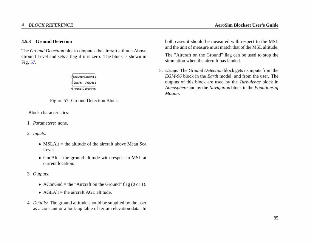
4 BLOCK REFERENCE AeroSim Blockset User’s Guide
4.5.3 Ground Detection
TheGround Detectionblock computes the aircraft altitude AboveGround Level and sets a flag if it is zero. The block is shown inFig. 57.
Figure 57: Ground Detection Block
Block characteristics:
1. Parameters:none.
2. Inputs:
• MSLAlt = the altitude of the aircraft above Mean SeaLevel.
• GndAlt = the ground altitude with respect to MSL atcurrent location.
3. Outputs:
• AConGnd = the ”Aircraft on the Ground” flag (0 or 1).
• AGLAlt = the aircraft AGL altitude.
4. Details: The ground altitude should be supplied by the useras a constant or a look-up table of terrain elevation data. In
both cases it should be measured with respect to the MSLand the unit of measure must match that of the MSL altitude.
The ”Aircraft on the Ground” flag can be used to stop thesimulation when the aircraft has landed.
5. Usage:TheGround Detectionblock gets its inputs from theEGM-96block in theEarth model, and from the user. Theoutputs of this block are used by theTurbulenceblock inAtmosphereand by theNavigationblock in theEquations ofMotion.
85
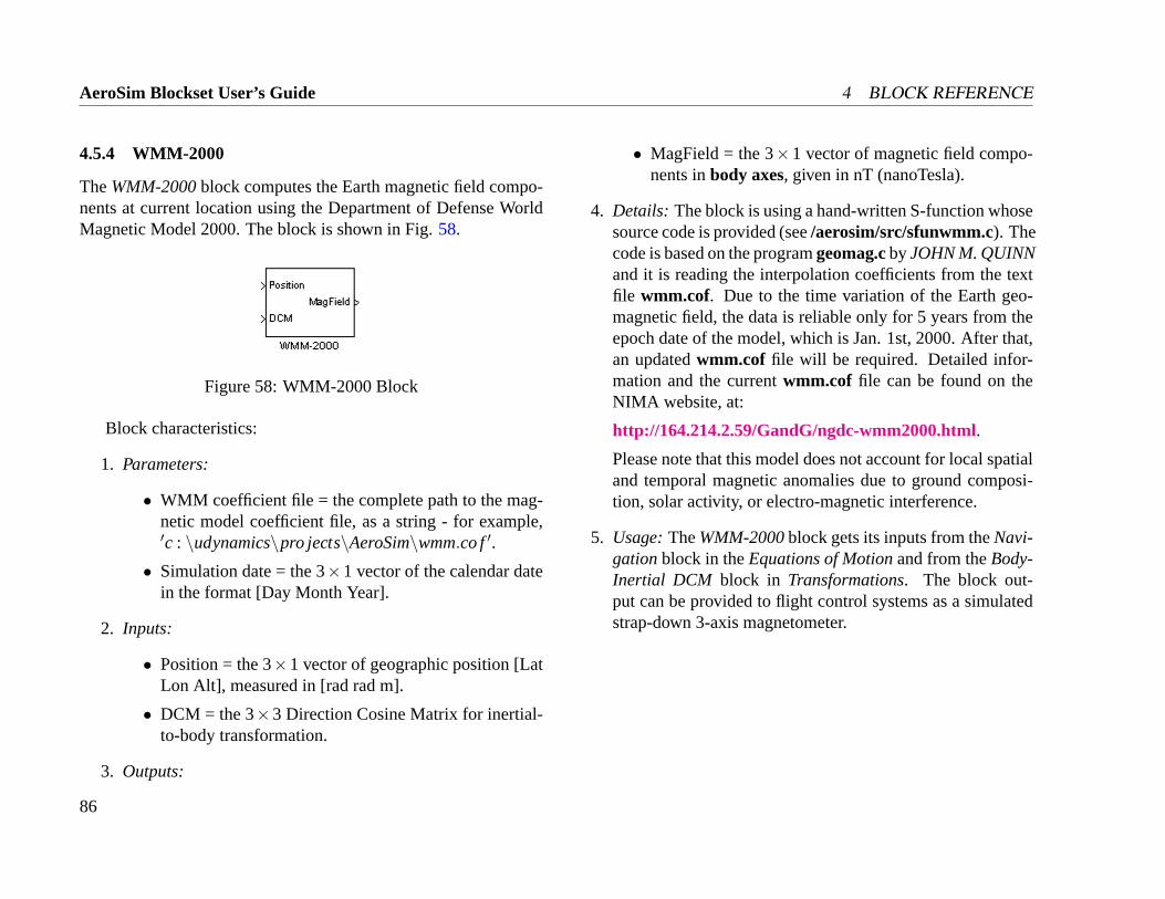
AeroSim Blockset User’s Guide 4 BLOCK REFERENCE
4.5.4 WMM-2000
TheWMM-2000block computes the Earth magnetic field compo-nents at current location using the Department of Defense WorldMagnetic Model 2000. The block is shown in Fig.58.
Figure 58: WMM-2000 Block
Block characteristics:
1. Parameters:
• WMM coefficient file = the complete path to the mag-netic model coefficient file, as a string - for example,′c : \udynamics\pro jects\AeroSim\wmm.co f′.
• Simulation date = the 3×1 vector of the calendar datein the format [Day Month Year].
2. Inputs:
• Position = the 3×1 vector of geographic position [LatLon Alt], measured in [rad rad m].
• DCM = the 3×3 Direction Cosine Matrix for inertial-to-body transformation.
3. Outputs:
• MagField = the 3×1 vector of magnetic field compo-nents inbody axes, given in nT (nanoTesla).
4. Details: The block is using a hand-written S-function whosesource code is provided (see/aerosim/src/sfunwmm.c). Thecode is based on the programgeomag.cbyJOHN M. QUINNand it is reading the interpolation coefficients from the textfile wmm.cof. Due to the time variation of the Earth geo-magnetic field, the data is reliable only for 5 years from theepoch date of the model, which is Jan. 1st, 2000. After that,an updatedwmm.cof file will be required. Detailed infor-mation and the currentwmm.cof file can be found on theNIMA website, at:
http://164.214.2.59/GandG/ngdc-wmm2000.html.
Please note that this model does not account for local spatialand temporal magnetic anomalies due to ground composi-tion, solar activity, or electro-magnetic interference.
5. Usage:TheWMM-2000block gets its inputs from theNavi-gationblock in theEquations of Motionand from theBody-Inertial DCM block in Transformations. The block out-put can be provided to flight control systems as a simulatedstrap-down 3-axis magnetometer.
86
4 BLOCK REFERENCE AeroSim Blockset User’s Guide
4.6 Equations of Motion
The Equations of Motion library folder includes blocks for allof the differential equations that describe the dynamics of the air-craft. These equations form the centerpiece of an aircraft dynamicmodel. There are two formulations for the equations of motionthat are commonly used, and they are provided in two separatesub-folders within the AeroSim library. These are: the EOM withvelocities in body axes (XYZ), and the EOM with aircraft veloc-ities in geodetic frame (NED). From I/O point-of-view, both for-mulations provide the same inputs and outputs (for example, bothwill output velocities in body frame AND in geodetic frame) suchthat the designer can easily switch to a different EOM formulationafter the aircraft model has already been built.
87

AeroSim Blockset User’s Guide 4 BLOCK REFERENCE
4.6.1 Total Acceleration
The block adds all accelerations applied to the airframe due toaerodynamics and propulsion, and returns the sum as body-axescomponents. The block is shown in Fig.59.
Figure 59: Total Acceleration Block
Block characteristics:
1. Parameters:none.
2. Inputs:
• Faero = the 3×1 vector of aerodynamic forces in bodyaxes[Fxaero Fyaero Fzaero]
T .
• Fprop = the 3×1 vector of propulsion forces in bodyaxes
[Fxprop Fyprop Fzprop
]T.
• Mass = the current aircraft mass.
3. Outputs:
• Acc = the 3× 1 vector of total acceleration in body-axes[ax ay az]
T .
4. Details: The ”total acceleration” includes everything exceptthe gravity. Potential forces like gravity cannot be sensedby accelerometers since they affect all of the accelerometersub-components in the same way. The total accelerationsare computed simply as:ax
ay
az
applied
=1
Maircra f t·
Fx
Fy
Fz
aero
+
Fx
Fy
Fz
prop
(32)
5. Usage:The block inputs are provided by theAerodynamicForceblock inAerodynamics, thePropulsion Forceblock inPropulsionand theAircraft Inertia block. The total acceler-ation output is used by theForcesblock in theEquations ofMotion and it can also be provided as aircraft model outputin order to simulate a 3-axis accelerometer system.
88
4 BLOCK REFERENCE AeroSim Blockset User’s Guide
4.6.2 Total Moment
The block computes the total moment applied to the airframe bythe aerodynamics and propulsion. The moment is computed aboutthe current aircraft CG location. The block is shown in Fig.60.
Figure 60: Total Moment Block
Block characteristics:
1. Parameters:
• Aerodynamic force application point = the coordinatesof the point at which the aerodynamic forces and mo-ments are given, in body axesraero= [Xaero Yaero Zaero]
T .
• Propulsion force application point = the coordinates ofthe point at which the propulsion forces and momentsare given, in body axesrprop= [Xprop Yprop Zprop]T .
2. Inputs:
• Faero = the 3×1 vector of aerodynamic forces in bodyaxesFaero = [Fxaero Fyaero Fzaero]
T .
• Maero = the 3×1 vector of aerodynamic moments inbody axesMaero = [Mxaero Myaero Mzaero]
T .
• Fprop = the 3×1 vector of propulsion forces in bodyaxesFprop =
[Fxprop Fyprop Fzprop
]T.
• Mprop = the 3× 1 vector of propulsion moments inbody axesMprop =
[Mxprop Myprop Mzprop
]T.
• CGpos = the 3× 1 vector of current CG position inbody axesrCG = [XCG YCG ZCG]T .
3. Outputs:
• Mcg = the 3×1 vector of total moment about the CGMCG = [Mx My Mz]
T .
4. Details: The total moment is computed as shown below:
MCG = (raero− rCG)×Faero+Maero+(rprop− rCG)×Fprop+
+Mprop(33)
5. Usage:The block inputs are provided byAerodynamic ForceandAerodynamic Momentin Aerodynamics, by PropulsionForceandPropulsion Momentin Propulsionand byAircraftInertia block in theInertia model. The block output is usedby theMomentsblock in theEquations of Motion.
89
AeroSim Blockset User’s Guide 4 BLOCK REFERENCE
4.6.3 Body-frame EOM: Forces
The block implements the rigid-body 6 degree-of-freedom forceequations that describe the time variation of the aircraft velocities.The block is shown in Fig.61.
Figure 61: Forces Block
Block characteristics:
1. Parameters:
• Initial velocities = the 3×1 vector of initial body ve-locities[u0 v0 w0 ]T .
2. Inputs:
• Rates = the 3×1 vector of body angular rates[ p q r]T .
• Accel = the 3×1 vector of body accelerations[ax ay az]T .
• Gravity = the gravitational acceleration as a scalar.
• DCM = the 3× 3 frame transformation matrix (fromnavigation (geodetic) to platform (body) frame.
• RST = the integrator reset flag, which can be 0 or 1.
3. Outputs:
• Velocities = the 3×1 vector of body velocities[u v w]T .
4. Details: The force equations implemented can be found in[3] and they are presented below:
u = rv−qw+gx +ax
v =−ru+ pw+gy +ay
w = qu− pv+gz+az
(34)
where: gx
gy
gz
= Rn2p ·
00g
(35)
The initial condition for the integration of velocities is takenfrom the block parameters. If the reset flag changes from0 to 1 during the simulation the integrator is reset back tothe initial condition. The accelerationsax, ay, andaz mustinclude all the airframe loads (aerodynamics, propulsion,winds). Please note that the body velocities include the windeffects; in other words, they represent the ground speed ofthe airplane expressed in body axes.
5. Usage:The block takes its inputs from theMomentsblockin Equations of Motion, from Total Accelerationblock intheInertia model, and from theWGS-84Earth geoid model.The reset flag can be handled by the user. The block outputis part of the aircraft state vector and it is used extensivelythroughout the aircraft model.
90
4 BLOCK REFERENCE AeroSim Blockset User’s Guide
4.6.4 Body-frame EOM: Moments
The block integrates the rigid-body 6 degree-of-freedom momentequations to obtain the instantaneous body angular rates. Theblock is presented in Fig.62.
Figure 62: Moments Block
Block characteristics:
1. Parameters:
• Initial angular rates = the 3×1 vector of initial bodyangular rates[ p0 q0 r0 ]T .
2. Inputs:
• Inertia = the 4×1 vector of current moments of inertia[Jx Jy Jz Jxz]
T .
• Moments = the 3×1 vector of airframe moments withrespect to the CG[L M N ]T .
• RST = the integrator reset flag, which can be 0 or 1.
3. Outputs:
• Angular Rates = the 3×1 vector of body angular rates[ p q r]T .
• Angular Acc = the 3×1 vector of body angular accel-erations[ p q r ]T .
4. Details: The moment equations are implemented as shownin [3]. A summary of the equations is given below:
p = (c1r +c2p)q+c3L+c4N
q = c5pr−c6(p2− r2
)+c7M
r = (c8p−c2r)q+c4L+c9N
(36)
where the inertia coefficientsc1 - c9 are computed using theInertia Coefficientsblock available in theInertia section oftheAeroSim library. The moments should include all avail-able loads (i.e. aerodynamics, propulsion, winds) and theyshould be given with respect to the current location of air-craft CG. The initial condition for the integration is takenfrom the block parameters. If the reset flag changes from 0to 1 during the simulation the integrator is reset back to theinitial condition.
5. Usage: The block gets its inputs from theAircraft Inertiaand Total Momentblocks in theInertia model. The resetflag can be handled by the user. The block output is part ofthe aircraft state vector and it is used extensively throughoutthe aircraft model.
91
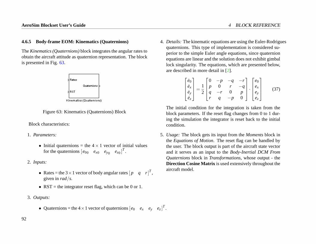
AeroSim Blockset User’s Guide 4 BLOCK REFERENCE
4.6.5 Body-frame EOM: Kinematics (Quaternions)
TheKinematics (Quaternions)block integrates the angular rates toobtain the aircraft attitude as quaternion representation. The blockis presented in Fig.63.
Figure 63: Kinematics (Quaternions) Block
Block characteristics:
1. Parameters:
• Initial quaternions = the 4×1 vector of initial valuesfor the quaternions[e00 ex0 ey0 ez0 ]T .
2. Inputs:
• Rates = the 3×1 vector of body angular rates[ p q r]T ,given inrad/s.
• RST = the integrator reset flag, which can be 0 or 1.
3. Outputs:
• Quaternions = the 4×1 vector of quaternions[e0 ex ey ez]T .
4. Details: The kinematic equations are using the Euler-Rodriguesquaternions. This type of implementation is considered su-perior to the simple Euler angle equations, since quaternionequations are linear and the solution does not exhibit gimballock singularity. The equations, which are presented below,are described in more detail in [2].
e0
ex
ey
ez
=12
0 −p −q −rp 0 r −qq −r 0 pr q −p 0
·
e0
ex
ey
ez
(37)
The initial condition for the integration is taken from theblock parameters. If the reset flag changes from 0 to 1 dur-ing the simulation the integrator is reset back to the initialcondition.
5. Usage:The block gets its input from theMomentsblock inthe Equations of Motion. The reset flag can be handled bythe user. The block output is part of the aircraft state vectorand it serves as an input to theBody-Inertial DCM FromQuaternionsblock in Transformations, whose output - theDirection Cosine Matrix is used extensively throughout theaircraft model.
92
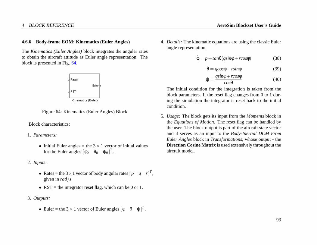
4 BLOCK REFERENCE AeroSim Blockset User’s Guide
4.6.6 Body-frame EOM: Kinematics (Euler Angles)
The Kinematics (Euler Angles)block integrates the angular ratesto obtain the aircraft attitude as Euler angle representation. Theblock is presented in Fig.64.
Figure 64: Kinematics (Euler Angles) Block
Block characteristics:
1. Parameters:
• Initial Euler angles = the 3×1 vector of initial valuesfor the Euler angles[φ0 θ0 ψ0 ]T .
2. Inputs:
• Rates = the 3×1 vector of body angular rates[ p q r]T ,given inrad/s.
• RST = the integrator reset flag, which can be 0 or 1.
3. Outputs:
• Euler = the 3×1 vector of Euler angles[φ θ ψ ]T .
4. Details: The kinematic equations are using the classic Eulerangle representation.
φ = p+ tanθ(qsinφ+ rcosφ) (38)
θ = qcosφ− rsinφ (39)
ψ =qsinφ+ rcosφ
cosθ(40)
The initial condition for the integration is taken from theblock parameters. If the reset flag changes from 0 to 1 dur-ing the simulation the integrator is reset back to the initialcondition.
5. Usage:The block gets its input from theMomentsblock inthe Equations of Motion. The reset flag can be handled bythe user. The block output is part of the aircraft state vectorand it serves as an input to theBody-Inertial DCM FromEuler Anglesblock in Transformations, whose output - theDirection Cosine Matrix is used extensively throughout theaircraft model.
93
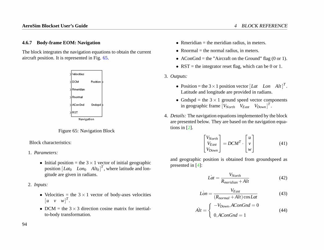
AeroSim Blockset User’s Guide 4 BLOCK REFERENCE
4.6.7 Body-frame EOM: Navigation
The block integrates the navigation equations to obtain the currentaircraft position. It is represented in Fig.65.
Figure 65: Navigation Block
Block characteristics:
1. Parameters:
• Initial position = the 3×1 vector of initial geographicposition[Lat0 Lon0 Alt0 ]T , where latitude and lon-gitude are given in radians.
2. Inputs:
• Velocities = the 3× 1 vector of body-axes velocities[u v w]T .
• DCM = the 3×3 direction cosine matrix for inertial-to-body transformation.
• Rmeridian = the meridian radius, in meters.
• Rnormal = the normal radius, in meters.
• AConGnd = the ”Aircraft on the Ground” flag (0 or 1).
• RST = the integrator reset flag, which can be 0 or 1.
3. Outputs:
• Position = the 3×1 position vector[Lat Lon Alt]T .Latitude and longitude are provided in radians.
• Gndspd = the 3× 1 ground speed vector componentsin geographic frame[VNorth VEast VDown]
T .
4. Details: The navigation equations implemented by the blockare presented below. They are based on the navigation equa-tions in [2]. VNorth
VEast
VDown
= DCMT ·
uvw
(41)
and geographic position is obtained from groundspeed aspresented in [4]:
˙Lat =VNorth
Rmeridian+Alt(42)
˙Lon=VEast
(Rnormal+Alt)cosLat(43)
Alt =
−VDown,AConGnd= 0
0,AConGnd= 1(44)
94
4 BLOCK REFERENCE AeroSim Blockset User’s Guide
The altitude integration depends on the status of the ”Air-craft on the Ground” flag.
5. Usage:TheNavigationblock gets its inputs from theForcesblock in Equations of Motion, Body-Inertial DCMblock inTransformations, WGS-84andGround Detectionblocks intheEarth model. The reset flag can be handled by the user.The position output is part of the aircraft state vector and itis used in theWGS-84, EGM-96, WMM-2000blocks in theEarth model, in theECEF Positionblock in Transforma-tions, and by theFS Interfaceblock in Pilot Interface. Thegroundspeed vector components are not used in the modelbut they can be output as simulated GPS velocity measure-ments.
95
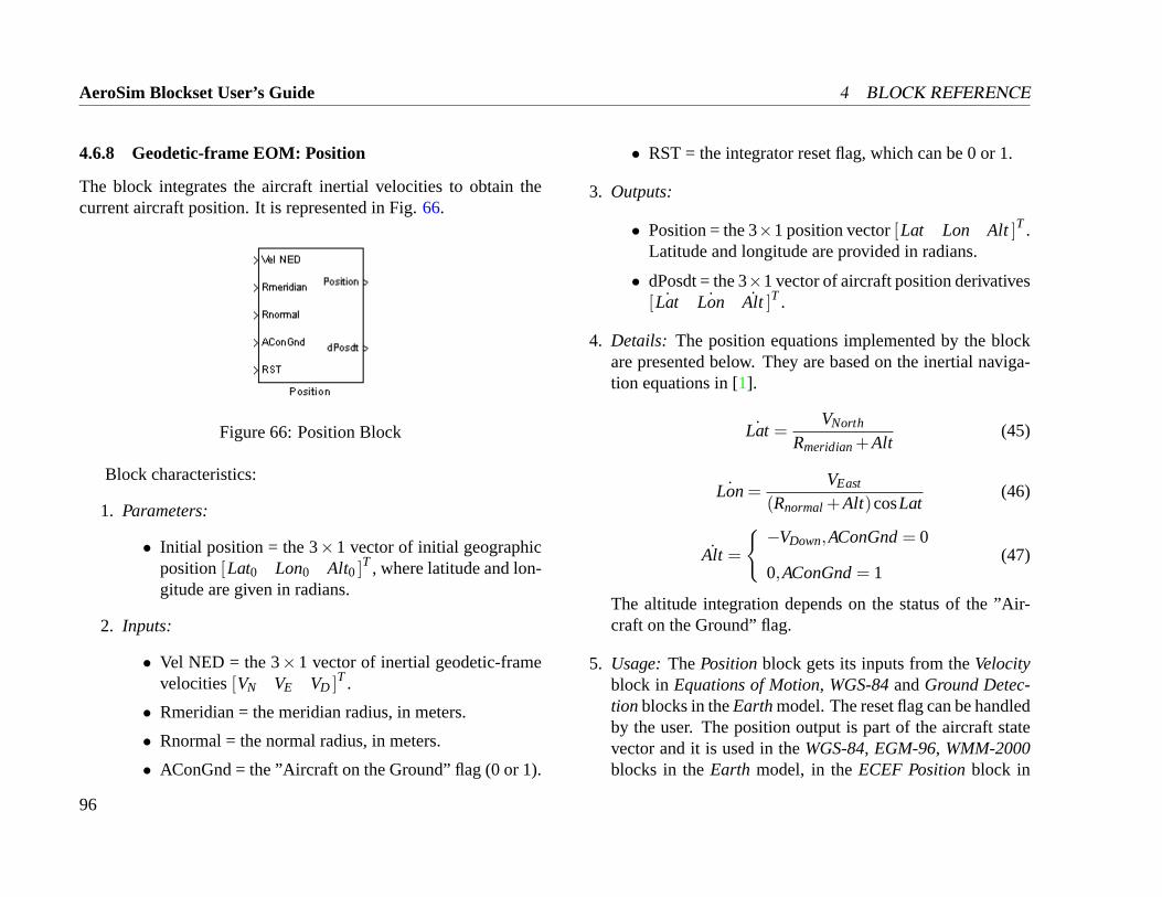
AeroSim Blockset User’s Guide 4 BLOCK REFERENCE
4.6.8 Geodetic-frame EOM: Position
The block integrates the aircraft inertial velocities to obtain thecurrent aircraft position. It is represented in Fig.66.
Figure 66: Position Block
Block characteristics:
1. Parameters:
• Initial position = the 3×1 vector of initial geographicposition[Lat0 Lon0 Alt0 ]T , where latitude and lon-gitude are given in radians.
2. Inputs:
• Vel NED = the 3×1 vector of inertial geodetic-framevelocities[VN VE VD ]T .
• Rmeridian = the meridian radius, in meters.
• Rnormal = the normal radius, in meters.
• AConGnd = the ”Aircraft on the Ground” flag (0 or 1).
• RST = the integrator reset flag, which can be 0 or 1.
3. Outputs:
• Position = the 3×1 position vector[Lat Lon Alt]T .Latitude and longitude are provided in radians.
• dPosdt = the 3×1 vector of aircraft position derivatives[ ˙Lat ˙Lon Alt ]T .
4. Details: The position equations implemented by the blockare presented below. They are based on the inertial naviga-tion equations in [1].
˙Lat =VNorth
Rmeridian+Alt(45)
˙Lon=VEast
(Rnormal+Alt)cosLat(46)
Alt =
−VDown,AConGnd= 0
0,AConGnd= 1(47)
The altitude integration depends on the status of the ”Air-craft on the Ground” flag.
5. Usage:ThePositionblock gets its inputs from theVelocityblock in Equations of Motion, WGS-84andGround Detec-tion blocks in theEarthmodel. The reset flag can be handledby the user. The position output is part of the aircraft statevector and it is used in theWGS-84, EGM-96, WMM-2000blocks in theEarth model, in theECEF Positionblock in
96
4 BLOCK REFERENCE AeroSim Blockset User’s Guide
Transformations, and by theFS Interfaceblock in Pilot In-terface. The position derivatives are used by theVelocityandtheAngular Rateblocks in theEquations of Motion.
97
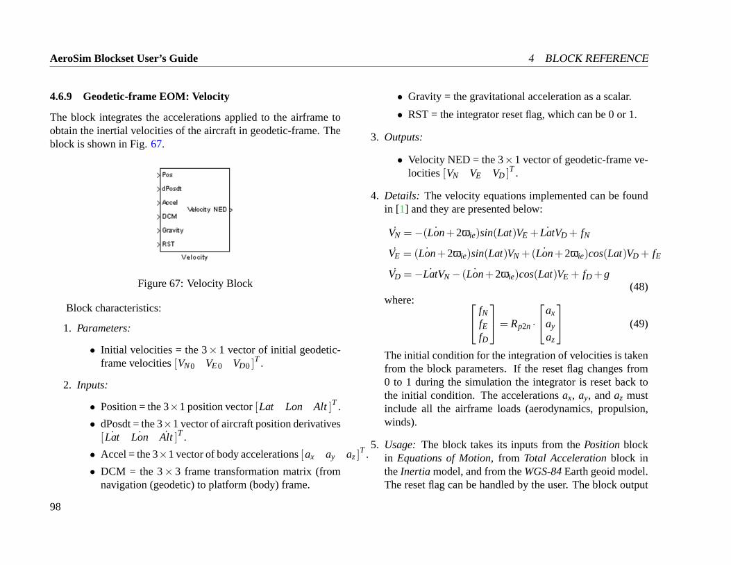
AeroSim Blockset User’s Guide 4 BLOCK REFERENCE
4.6.9 Geodetic-frame EOM: Velocity
The block integrates the accelerations applied to the airframe toobtain the inertial velocities of the aircraft in geodetic-frame. Theblock is shown in Fig.67.
Figure 67: Velocity Block
Block characteristics:
1. Parameters:
• Initial velocities = the 3×1 vector of initial geodetic-frame velocities[VN0 VE0 VD0 ]T .
2. Inputs:
• Position = the 3×1 position vector[Lat Lon Alt]T .
• dPosdt = the 3×1 vector of aircraft position derivatives[ ˙Lat ˙Lon Alt ]T .
• Accel = the 3×1 vector of body accelerations[ax ay az]T .
• DCM = the 3× 3 frame transformation matrix (fromnavigation (geodetic) to platform (body) frame.
• Gravity = the gravitational acceleration as a scalar.
• RST = the integrator reset flag, which can be 0 or 1.
3. Outputs:
• Velocity NED = the 3×1 vector of geodetic-frame ve-locities[VN VE VD ]T .
4. Details: The velocity equations implemented can be foundin [1] and they are presented below:
VN =−( ˙Lon+2ωie)sin(Lat)VE + ˙LatVD + fN
VE = ( ˙Lon+2ωie)sin(Lat)VN +( ˙Lon+2ωie)cos(Lat)VD + fE
VD =− ˙LatVN− ( ˙Lon+2ωie)cos(Lat)VE + fD +g(48)
where: fNfEfD
= Rp2n ·
ax
ay
az
(49)
The initial condition for the integration of velocities is takenfrom the block parameters. If the reset flag changes from0 to 1 during the simulation the integrator is reset back tothe initial condition. The accelerationsax, ay, andaz mustinclude all the airframe loads (aerodynamics, propulsion,winds).
5. Usage: The block takes its inputs from thePositionblockin Equations of Motion, from Total Accelerationblock intheInertia model, and from theWGS-84Earth geoid model.The reset flag can be handled by the user. The block output
98
4 BLOCK REFERENCE AeroSim Blockset User’s Guide
is part of the aircraft state vector and it is used extensivelythroughout the aircraft model.
99
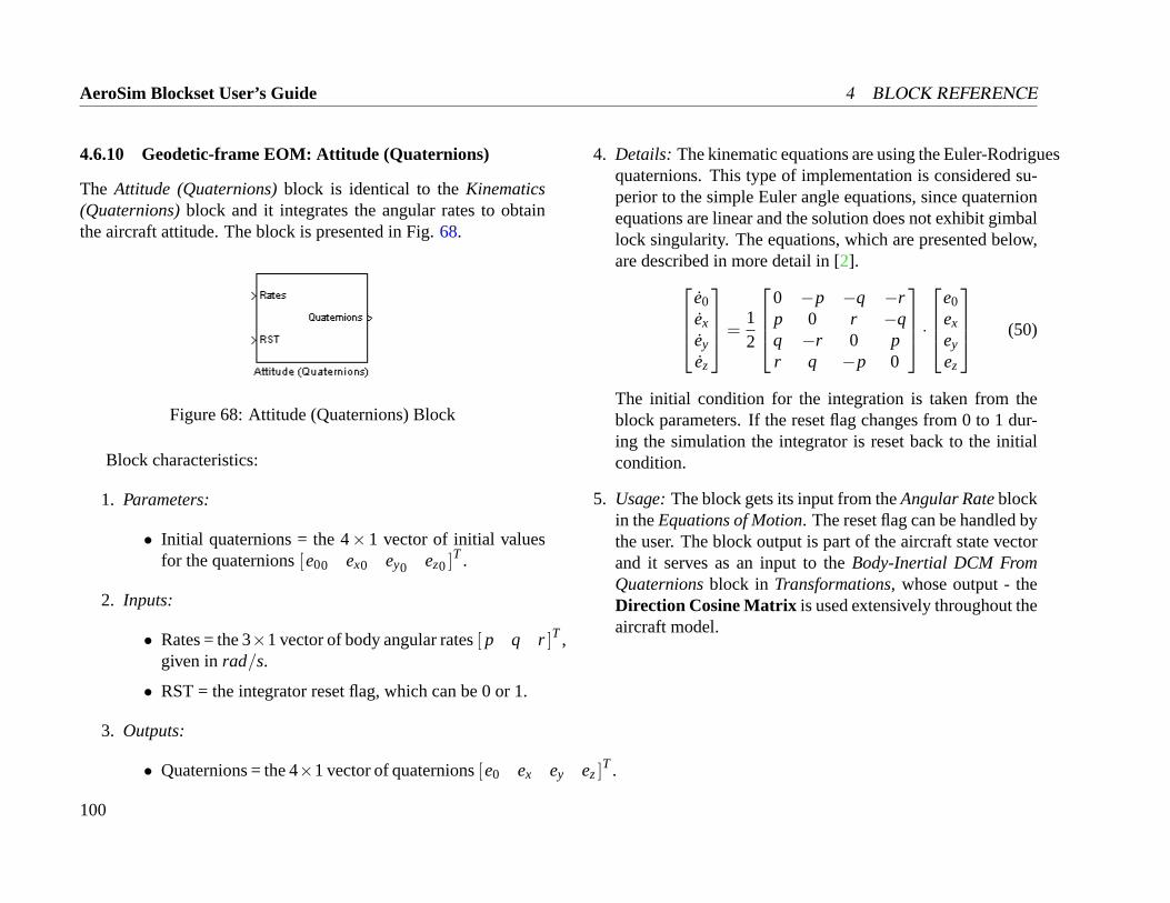
AeroSim Blockset User’s Guide 4 BLOCK REFERENCE
4.6.10 Geodetic-frame EOM: Attitude (Quaternions)
The Attitude (Quaternions)block is identical to theKinematics(Quaternions)block and it integrates the angular rates to obtainthe aircraft attitude. The block is presented in Fig.68.
Figure 68: Attitude (Quaternions) Block
Block characteristics:
1. Parameters:
• Initial quaternions = the 4×1 vector of initial valuesfor the quaternions[e00 ex0 ey0 ez0 ]T .
2. Inputs:
• Rates = the 3×1 vector of body angular rates[ p q r]T ,given inrad/s.
• RST = the integrator reset flag, which can be 0 or 1.
3. Outputs:
• Quaternions = the 4×1 vector of quaternions[e0 ex ey ez]T .
4. Details: The kinematic equations are using the Euler-Rodriguesquaternions. This type of implementation is considered su-perior to the simple Euler angle equations, since quaternionequations are linear and the solution does not exhibit gimballock singularity. The equations, which are presented below,are described in more detail in [2].
e0
ex
ey
ez
=12
0 −p −q −rp 0 r −qq −r 0 pr q −p 0
·
e0
ex
ey
ez
(50)
The initial condition for the integration is taken from theblock parameters. If the reset flag changes from 0 to 1 dur-ing the simulation the integrator is reset back to the initialcondition.
5. Usage:The block gets its input from theAngular Rateblockin theEquations of Motion. The reset flag can be handled bythe user. The block output is part of the aircraft state vectorand it serves as an input to theBody-Inertial DCM FromQuaternionsblock in Transformations, whose output - theDirection Cosine Matrix is used extensively throughout theaircraft model.
100
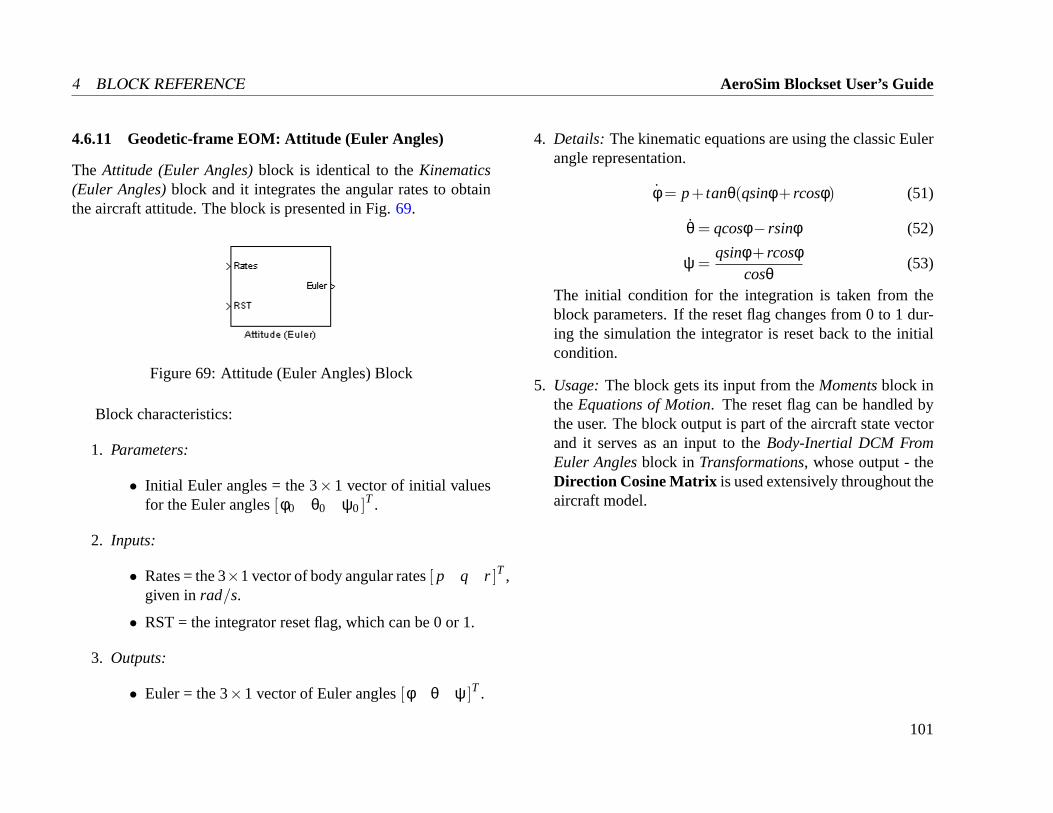
4 BLOCK REFERENCE AeroSim Blockset User’s Guide
4.6.11 Geodetic-frame EOM: Attitude (Euler Angles)
The Attitude (Euler Angles)block is identical to theKinematics(Euler Angles)block and it integrates the angular rates to obtainthe aircraft attitude. The block is presented in Fig.69.
Figure 69: Attitude (Euler Angles) Block
Block characteristics:
1. Parameters:
• Initial Euler angles = the 3×1 vector of initial valuesfor the Euler angles[φ0 θ0 ψ0 ]T .
2. Inputs:
• Rates = the 3×1 vector of body angular rates[ p q r]T ,given inrad/s.
• RST = the integrator reset flag, which can be 0 or 1.
3. Outputs:
• Euler = the 3×1 vector of Euler angles[φ θ ψ ]T .
4. Details: The kinematic equations are using the classic Eulerangle representation.
φ = p+ tanθ(qsinφ+ rcosφ) (51)
θ = qcosφ− rsinφ (52)
ψ =qsinφ+ rcosφ
cosθ(53)
The initial condition for the integration is taken from theblock parameters. If the reset flag changes from 0 to 1 dur-ing the simulation the integrator is reset back to the initialcondition.
5. Usage:The block gets its input from theMomentsblock inthe Equations of Motion. The reset flag can be handled bythe user. The block output is part of the aircraft state vectorand it serves as an input to theBody-Inertial DCM FromEuler Anglesblock in Transformations, whose output - theDirection Cosine Matrix is used extensively throughout theaircraft model.
101
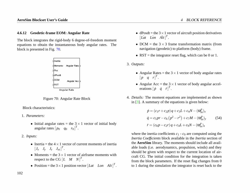
AeroSim Blockset User’s Guide 4 BLOCK REFERENCE
4.6.12 Geodetic-frame EOM: Angular Rate
The block integrates the rigid-body 6 degree-of-freedom momentequations to obtain the instantaneous body angular rates. Theblock is presented in Fig.70.
Figure 70: Angular Rate Block
Block characteristics:
1. Parameters:
• Initial angular rates = the 3×1 vector of initial bodyangular rates[ p0 q0 r0 ]T .
2. Inputs:
• Inertia = the 4×1 vector of current moments of inertia[Jx Jy Jz Jxz]
T .
• Moments = the 3×1 vector of airframe moments withrespect to the CG[L M N ]T .
• Position = the 3×1 position vector[Lat Lon Alt]T .
• dPosdt = the 3×1 vector of aircraft position derivatives[ ˙Lat ˙Lon Alt ]T .
• DCM = the 3× 3 frame transformation matrix (fromnavigation (geodetic) to platform (body) frame.
• RST = the integrator reset flag, which can be 0 or 1.
3. Outputs:
• Angular Rates = the 3×1 vector of body angular rates[ p q r]T .
• Angular Acc = the 3×1 vector of body angular accel-erations[ p q r ]T .
4. Details: The moment equations are implemented as shownin [3]. A summary of the equations is given below:
p = (c1r +c2p)q+c3L+c4N− (ωpin)x
q = c5pr−c6(p2− r2
)+c7M− (ωp
in)y
r = (c8p−c2r)q+c4L+c9N− (ωpin)z
(54)
where the inertia coefficientsc1 - c9 are computed using theInertia Coefficientsblock available in theInertia section oftheAeroSim library. The moments should include all avail-able loads (i.e. aerodynamics, propulsion, winds) and theyshould be given with respect to the current location of air-craft CG. The initial condition for the integration is takenfrom the block parameters. If the reset flag changes from 0to 1 during the simulation the integrator is reset back to the
102
4 BLOCK REFERENCE AeroSim Blockset User’s Guide
initial condition. Theωpin vector represents the Earth rota-
tion rate in body-axes and it can be computed as follows:
ωpin = Rn2p
( ˙Lon+ωie)cos(Lat)− ˙Lat
−( ˙Lon+ωie)sin(Lat)
(55)
5. Usage: The block gets its inputs from theAircraft InertiaandTotal Momentblocks in theInertia model, and from thePositionblock inEquations of Motion. The reset flag can behandled by the user. The block output is part of the aircraftstate vector and it is used extensively throughout the aircraftmodel.
103
AeroSim Blockset User’s Guide 4 BLOCK REFERENCE
4.7 Inertia
TheInertia library folder includes blocks that model the evolutionof the aircraft inertia parameters, including mass, CG position, andmoments of inertia. Also, the same folder includes the blocks thatsum-up all the forces and moments provided by the aerodynamic,propulsion, and atmospheric models to obtain a single force and asingle moment that can be used in the equations of motion.
104
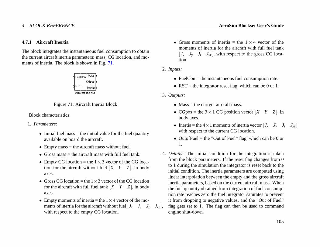
4 BLOCK REFERENCE AeroSim Blockset User’s Guide
4.7.1 Aircraft Inertia
The block integrates the instantaneous fuel consumption to obtainthe current aircraft inertia parameters: mass, CG location, and mo-ments of inertia. The block is shown in Fig.71.
Figure 71: Aircraft Inertia Block
Block characteristics:
1. Parameters:
• Initial fuel mass = the initial value for the fuel quantityavailable on board the aircraft.
• Empty mass = the aircraft mass without fuel.
• Gross mass = the aircraft mass with full fuel tank.
• Empty CG location = the 1×3 vector of the CG loca-tion for the aircraft without fuel[X Y Z], in bodyaxes.
• Gross CG location = the 1×3 vector of the CG locationfor the aircraft with full fuel tank[X Y Z], in bodyaxes.
• Empty moments of inertia = the 1×4 vector of the mo-ments of inertia for the aircraft without fuel[Jx Jy Jz Jxz],with respect to the empty CG location.
• Gross moments of inertia = the 1× 4 vector of themoments of inertia for the aircraft with full fuel tank[Jx Jy Jz Jxz], with respect to the gross CG loca-tion.
2. Inputs:
• FuelCon = the instantaneous fuel consumption rate.
• RST = the integrator reset flag, which can be 0 or 1.
3. Outputs:
• Mass = the current aircraft mass.
• CGpos = the 3×1 CG position vector[X Y Z], inbody axes.
• Inertia = the 4×1 moments of inertia vector[Jx Jy Jz Jxz]with respect to the current CG location.
• OutofFuel = the ”Out of Fuel” flag, which can be 0 or1.
4. Details: The initial condition for the integration is takenfrom the block parameters. If the reset flag changes from 0to 1 during the simulation the integrator is reset back to theinitial condition. The inertia parameters are computed usinglinear interpolation between the empty and the gross aircraftinertia parameters, based on the current aircraft mass. Whenthe fuel quantity obtained from integration of fuel consump-tion rate reaches zero the fuel integrator saturates to preventit from dropping to negative values, and the ”Out of Fuel”flag gets set to 1. The flag can then be used to commandengine shut-down.
105
AeroSim Blockset User’s Guide 4 BLOCK REFERENCE
5. Usage: The block input should be provided by the enginemodel. The reset flag can be handled by the user. The massoutput is used by theTotal accelerationblock in theIner-tia model and by theWind Forceblock in theAtmospheremodel. The CG position output is used by theTotal momentblock in theInertia model. TheInertia output is used by theMomentsequations in theEquations of Motionand by theWind Momentblock in theAtmospheremodel.
106
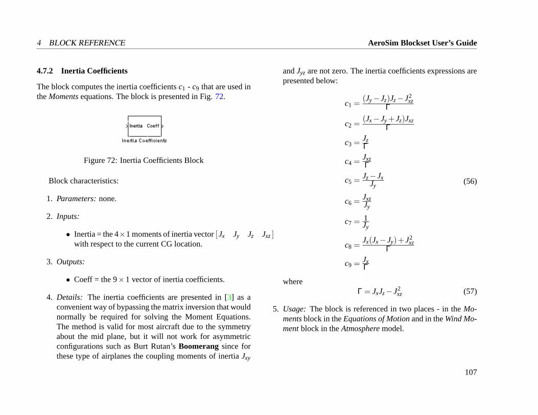
4 BLOCK REFERENCE AeroSim Blockset User’s Guide
4.7.2 Inertia Coefficients
The block computes the inertia coefficientsc1 - c9 that are used intheMomentsequations. The block is presented in Fig.72.
Figure 72: Inertia Coefficients Block
Block characteristics:
1. Parameters:none.
2. Inputs:
• Inertia = the 4×1 moments of inertia vector[Jx Jy Jz Jxz]with respect to the current CG location.
3. Outputs:
• Coeff = the 9×1 vector of inertia coefficients.
4. Details: The inertia coefficients are presented in [3] as aconvenient way of bypassing the matrix inversion that wouldnormally be required for solving the Moment Equations.The method is valid for most aircraft due to the symmetryabout the mid plane, but it will not work for asymmetricconfigurations such as Burt Rutan’sBoomerangsince forthese type of airplanes the coupling moments of inertiaJxy
andJyz are not zero. The inertia coefficients expressions arepresented below:
c1 =(Jy−Jz)Jz−J2
xzΓ
c2 =(Jx−Jy +Jz)Jxz
Γ
c3 = JzΓ
c4 = JxzΓ
c5 = Jz−JxJy
c6 = JxzJy
c7 = 1Jy
c8 =Jx(Jx−Jy)+J2
xzΓ
c9 = JxΓ
(56)
whereΓ = JxJz−J2
xz (57)
5. Usage: The block is referenced in two places - in theMo-mentsblock in theEquations of Motionand in theWind Mo-mentblock in theAtmospheremodel.
107
AeroSim Blockset User’s Guide 4 BLOCK REFERENCE
4.8 Math
This library folder includes all of the math functions that are ref-erenced by blocks in theAeroSim library.
108
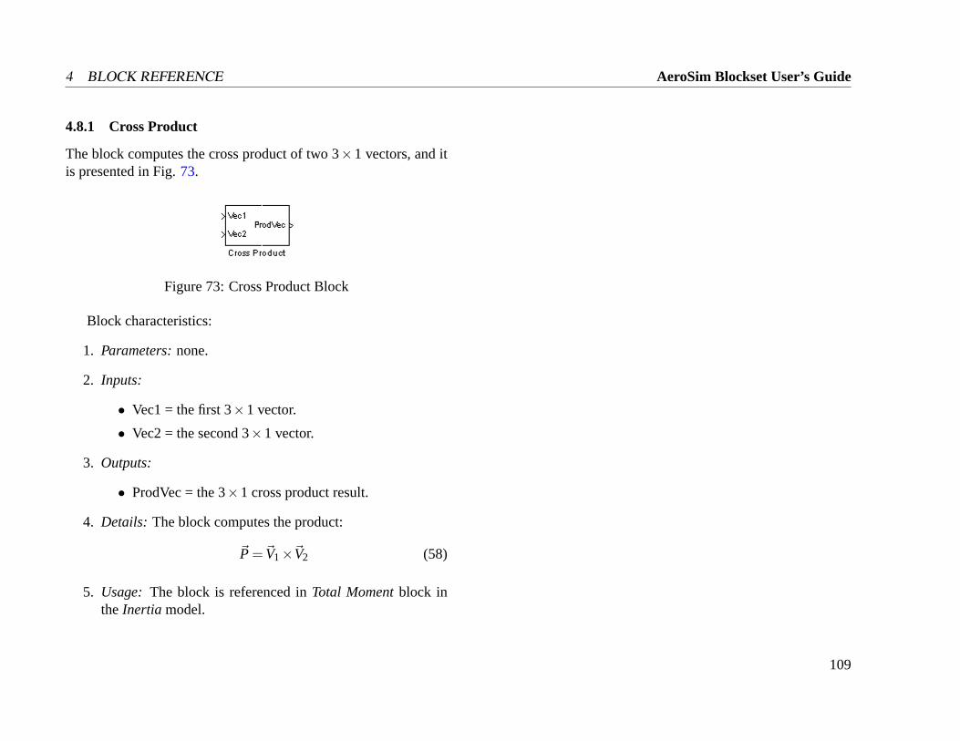
4 BLOCK REFERENCE AeroSim Blockset User’s Guide
4.8.1 Cross Product
The block computes the cross product of two 3×1 vectors, and itis presented in Fig.73.
Figure 73: Cross Product Block
Block characteristics:
1. Parameters:none.
2. Inputs:
• Vec1 = the first 3×1 vector.
• Vec2 = the second 3×1 vector.
3. Outputs:
• ProdVec = the 3×1 cross product result.
4. Details: The block computes the product:
~P =~V1×~V2 (58)
5. Usage: The block is referenced inTotal Momentblock intheInertia model.
109
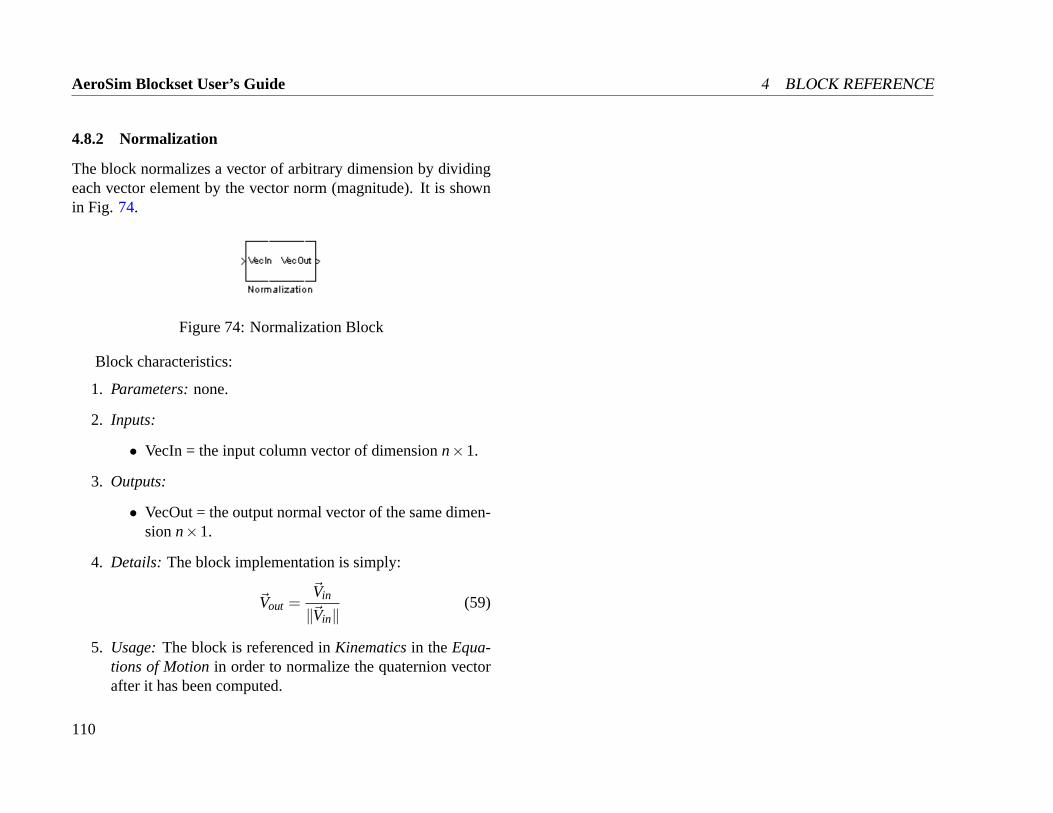
AeroSim Blockset User’s Guide 4 BLOCK REFERENCE
4.8.2 Normalization
The block normalizes a vector of arbitrary dimension by dividingeach vector element by the vector norm (magnitude). It is shownin Fig. 74.
Figure 74: Normalization Block
Block characteristics:
1. Parameters:none.
2. Inputs:
• VecIn = the input column vector of dimensionn×1.
3. Outputs:
• VecOut = the output normal vector of the same dimen-sionn×1.
4. Details: The block implementation is simply:
~Vout =~Vin
‖~Vin‖(59)
5. Usage:The block is referenced inKinematicsin theEqua-tions of Motionin order to normalize the quaternion vectorafter it has been computed.
110
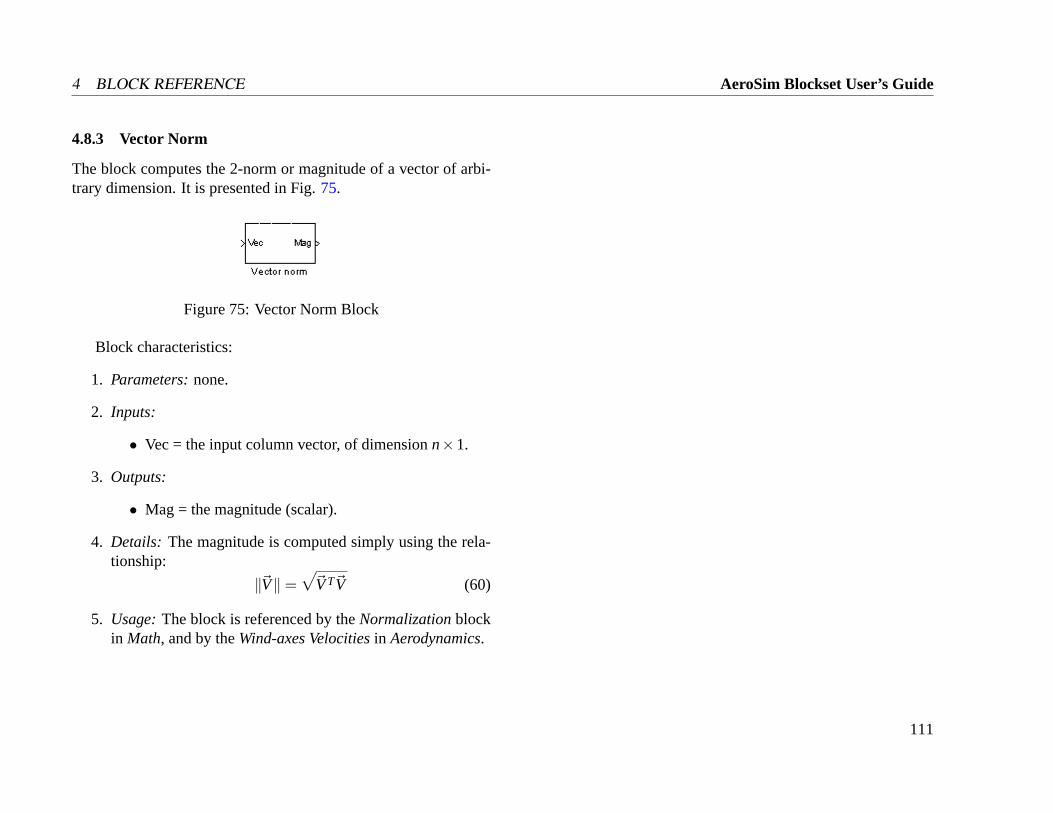
4 BLOCK REFERENCE AeroSim Blockset User’s Guide
4.8.3 Vector Norm
The block computes the 2-norm or magnitude of a vector of arbi-trary dimension. It is presented in Fig.75.
Figure 75: Vector Norm Block
Block characteristics:
1. Parameters:none.
2. Inputs:
• Vec = the input column vector, of dimensionn×1.
3. Outputs:
• Mag = the magnitude (scalar).
4. Details: The magnitude is computed simply using the rela-tionship:
‖~V‖ =√
~VT~V (60)
5. Usage:The block is referenced by theNormalizationblockin Math, and by theWind-axes Velocitiesin Aerodynamics.
111
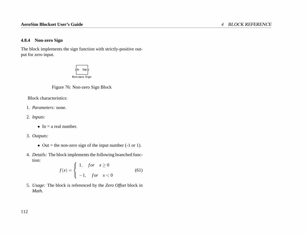
AeroSim Blockset User’s Guide 4 BLOCK REFERENCE
4.8.4 Non-zero Sign
The block implements the sign function with strictly-positive out-put for zero input.
Figure 76: Non-zero Sign Block
Block characteristics:
1. Parameters:none.
2. Inputs:
• In = a real number.
3. Outputs:
• Out = the non-zero sign of the input number (-1 or 1).
4. Details: The block implements the following branched func-tion:
f (x) =
1, f or x≥ 0
−1, f or x < 0(61)
5. Usage:The block is referenced by theZero Offsetblock inMath.
112
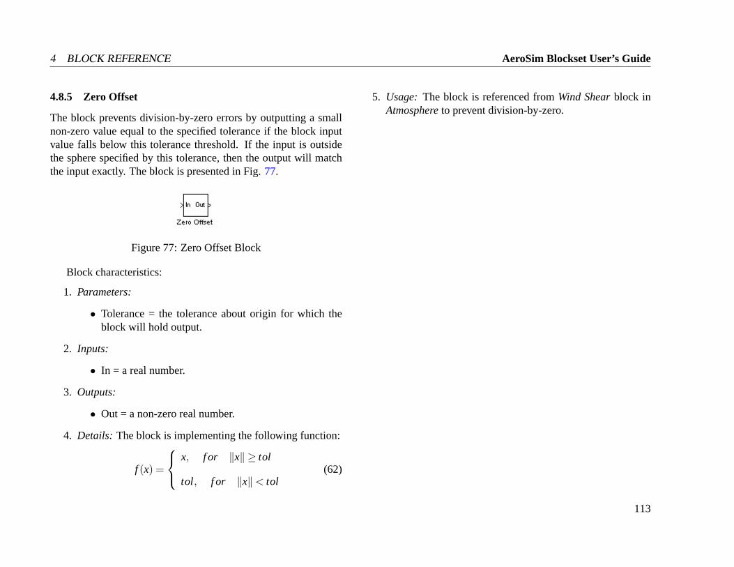
4 BLOCK REFERENCE AeroSim Blockset User’s Guide
4.8.5 Zero Offset
The block prevents division-by-zero errors by outputting a smallnon-zero value equal to the specified tolerance if the block inputvalue falls below this tolerance threshold. If the input is outsidethe sphere specified by this tolerance, then the output will matchthe input exactly. The block is presented in Fig.77.
Figure 77: Zero Offset Block
Block characteristics:
1. Parameters:
• Tolerance = the tolerance about origin for which theblock will hold output.
2. Inputs:
• In = a real number.
3. Outputs:
• Out = a non-zero real number.
4. Details: The block is implementing the following function:
f (x) =
x, f or ‖x‖ ≥ tol
tol, f or ‖x‖ < tol(62)
5. Usage: The block is referenced fromWind Shearblock inAtmosphereto prevent division-by-zero.
113
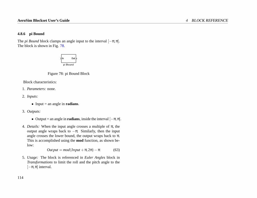
AeroSim Blockset User’s Guide 4 BLOCK REFERENCE
4.8.6 pi Bound
Thepi Boundblock clamps an angle input to the interval[−π,π].The block is shown in Fig.78.
Figure 78: pi Bound Block
Block characteristics:
1. Parameters:none.
2. Inputs:
• Input = an angle inradians.
3. Outputs:
• Output = an angle inradians, inside the interval[−π,π].
4. Details: When the input angle crosses a multiple ofπ, theoutput angle wraps back to−π. Similarly, then the inputangle crosses the lower bound, the output wraps back toπ.This is accomplished using themod function, as shown be-low:
Out put= mod(Input+π,2π)−π (63)
5. Usage: The block is referenced inEuler Anglesblock inTransformationsto limit the roll and the pitch angle to the[−π,π] interval.
114
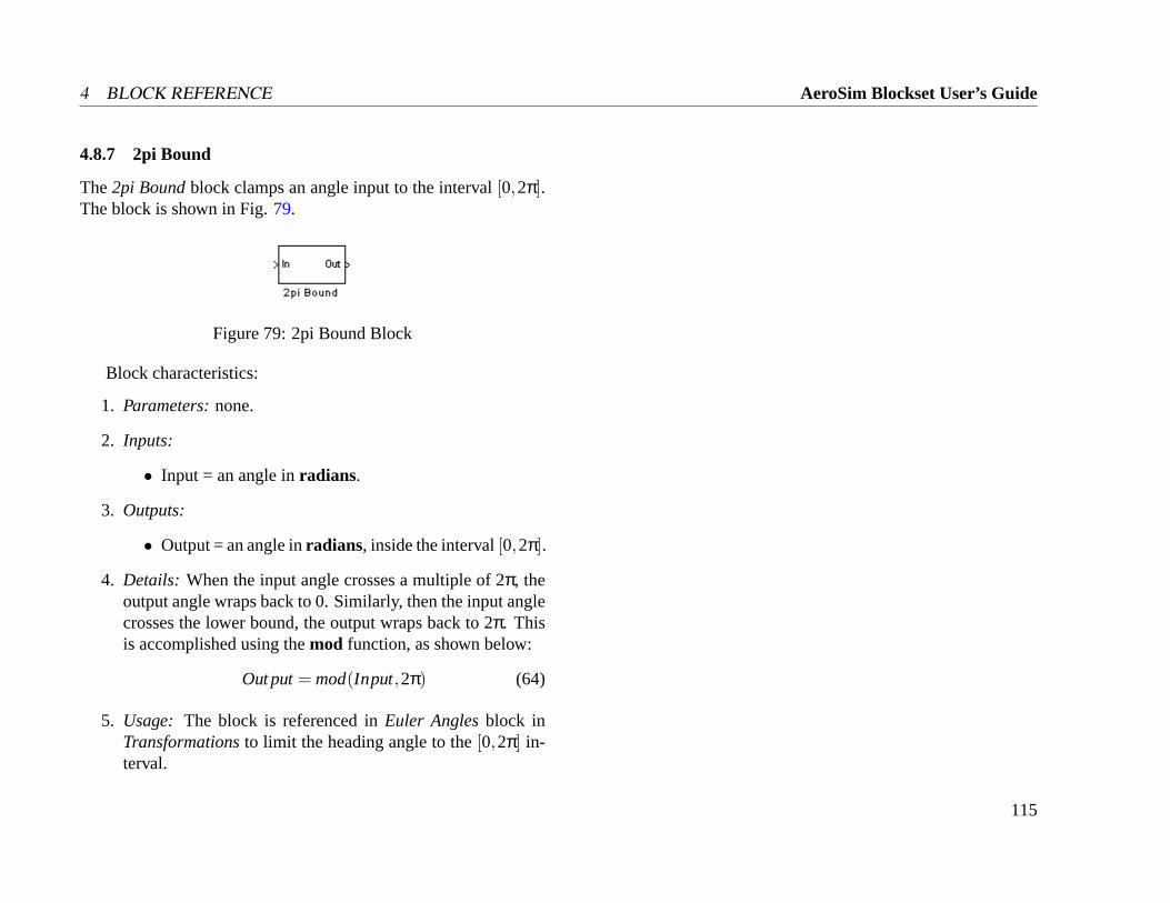
4 BLOCK REFERENCE AeroSim Blockset User’s Guide
4.8.7 2pi Bound
The2pi Boundblock clamps an angle input to the interval[0,2π].The block is shown in Fig.79.
Figure 79: 2pi Bound Block
Block characteristics:
1. Parameters:none.
2. Inputs:
• Input = an angle inradians.
3. Outputs:
• Output = an angle inradians, inside the interval[0,2π].
4. Details: When the input angle crosses a multiple of 2π, theoutput angle wraps back to 0. Similarly, then the input anglecrosses the lower bound, the output wraps back to 2π. Thisis accomplished using themod function, as shown below:
Out put= mod(Input,2π) (64)
5. Usage: The block is referenced inEuler Anglesblock inTransformationsto limit the heading angle to the[0,2π] in-terval.
115
AeroSim Blockset User’s Guide 4 BLOCK REFERENCE
4.9 Pilot Interface
ThePilot Interface library folder includes input and output driversfor devices outside theMatlab/Simulink environment, throughwhich the user can interact with the aircraft model.
116
4 BLOCK REFERENCE AeroSim Blockset User’s Guide
4.9.1 FS Interface
The block provides an interface toMicrosoft Flight Simulatorfor a real-time visual display of the aircraft. The block is shown inFig. 80.
Figure 80: FS Interface Block
Block characteristics:
1. Parameters:
• Sample time = the sample time at which position andattitude data will be sent toMicrosoft Flight Simula-tor .
2. Inputs:
• Position = the 3×1 vector of geographic position [LatLon Alt] in [rad rad m] .
• Euler = the 3×1 vector of Euler angles[φ θ ψ ]T
in radians.
• Airspeed = the current aircraft airspeed, inm/s.
3. Outputs: no output signals to Simulink, only visual outputin Microsoft Flight Simulator .
4. Details: The block is implemented using the CMEX S-functionsfunflightsim.dll. The mechanism through whichMSFSstate variables are accessed and written is by using Inter-Process Communication provided byFSUIPC utility by Pe-ter L. Dowson. The modulefsuipc.dll has to be installedin Microsoft Flight Simulator . TheMSFS state variablesare then accessed using the functions available in the libraryIPCuser.c. Memory addresses of these state variables aredefined inFSUIPC User.h.
The S-function provided with theFS Interfaceblock is over-writing the aircraft position, attitude, and airspeed variablesin Microsoft Flight Simulator to provide a visual displayof the aircraft behavior. To prevent interference withMSFS’own aircraft dynamics,MSFSshould be run in SLEW mode.When starting the simulation, theFS Interfaceblock willenable the SLEW mode automatically. The disadvantage isthat some instruments in the aircraft cockpit panel displayedin MSFS are not updated in this mode. However, the mainobjective - displaying an outside view of the aircraft - is ac-complished, see Fig.81.
BothMatlab/Simulink andMicrosoft Flight Simulator arecomputationally-intensive applications. Although it is pos-sible to run both on the same computer, we recommend ex-ecuting them on separate machines. The way this can bedone is by making use of theWideFS utility by Peter L.Dowson. This Client/Server application allows remote ac-cess toMSFS state variables usingFSUIPC. This requiresthe installation ofwideserver.dll in addition tofsuipc.dll ontheMSFS machine, and the execution ofwideclient.exeon
117
AeroSim Blockset User’s Guide 4 BLOCK REFERENCE
Figure 81: Aerosonde in a simulated weather recon flight
theMatlab/Simulink machine.
Latest versions ofFSUIPC and WIDEFS can be down-loaded at:
http://www.flightsim.com.
5. Usage:TheFS Interfaceblock gets its inputs from theNav-igation block in Equations of Motion, from Euler Anglesblock inTransformationsand fromWind-axes Velocitiesblockin Aerodynamics. The only block output is visual and it re-quires the presence ofMicrosoft Flight Simulator on thelocal machine or on a secondary machine on the local net-work.
118
4 BLOCK REFERENCE AeroSim Blockset User’s Guide
4.9.2 FlightGear Interface
The block provides an interface toFlightGear Flight Simulatorfor a real-time visual display of the aircraft. The block is shown inFig. 82.
Figure 82: FlightGear Interface Block
Block characteristics:
1. Parameters:
• Host name = the name or IP address of the machine onwhich FlightGear is running, provided as a string. Forexample, if we want to run both Matlab and FlightGearon the same computer (not recommended performance-wise) we would use’localhost’.Otherwise, we can typea ’hostname’ or an IP address’192.168.0.247’.
• Sample time = the sample time at which position andattitude data will be sent toFlightGear Flight Simu-lator .
2. Inputs:
• Position = the 3×1 vector of geographic position [LatLon Alt] in [rad rad m] .
• Euler = the 3×1 vector of Euler angles[φ θ ψ ]T
in radians.
• Airspeed = the current aircraft airspeed, inm/s.
3. Outputs: no output signals to Simulink, only visual outputin FlightGear Flight Simulator .
4. Details: The block is implemented using the CMEX S-functionsfunflightgear.dll. Data is being sent toFlightGear usingthe UDP network protocol, on port 5500. To set-up Flight-Gear for accepting external aircraft model over the UDPconnection, you must run its executable with the followingcommand line arguments:
%FG_ROOT%\BIN\FGFS.EXE --disable-splash-screen--native-fdm=socket,in,30,,5500,udp --fdm=external
A screen capture of the visual output is shown in Fig.83.
Both Matlab/Simulink andFlightGear Flight Simulatorare computationally-intensive applications. Although it ispossible to run both on the same computer, we recommendexecuting them on separate machines. The version ofFlight-Gear Flight Simulator supported by this S-function is 0.8.OtherFlightGear Flight Simulator releases can be used,but in this case the S-functionsfunflightgear.dll will haveto be recompiled using thenet fdm.hxx from the Flight-Gear Flight Simulator source tree. Latest version can bedownloaded at:
http://www.flightgear.org .
119
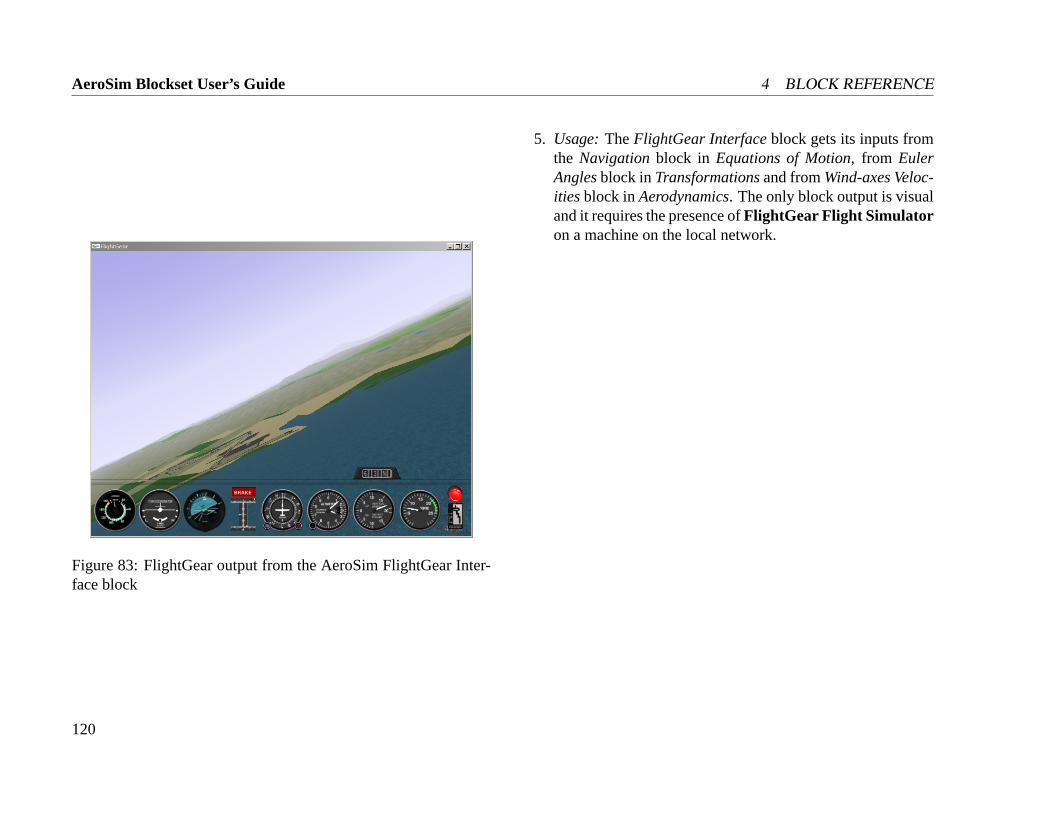
AeroSim Blockset User’s Guide 4 BLOCK REFERENCE
Figure 83: FlightGear output from the AeroSim FlightGear Inter-face block
5. Usage:TheFlightGear Interfaceblock gets its inputs fromthe Navigationblock in Equations of Motion, from EulerAnglesblock inTransformationsand fromWind-axes Veloc-itiesblock inAerodynamics. The only block output is visualand it requires the presence ofFlightGear Flight Simulatoron a machine on the local network.
120
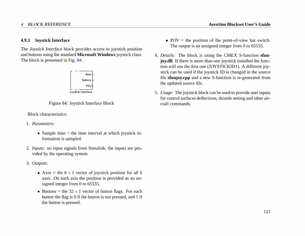
4 BLOCK REFERENCE AeroSim Blockset User’s Guide
4.9.3 Joystick Interface
The Joystick Interfaceblock provides access to joystick positionand buttons using the standardMicrosoft Windows joystick class.The block is presented in Fig.84.
Figure 84: Joystick Interface Block
Block characteristics:
1. Parameters:
• Sample time = the time interval at which joystick in-formation is sampled.
2. Inputs: no input signals from Simulink, the inputs are pro-vided by the operating system.
3. Outputs:
• Axes = the 6× 1 vector of joystick position for all 6axes. On each axis the position is provided as an un-signed integer from 0 to 65535.
• Buttons = the 32×1 vector of button flags. For eachbutton the flag is 0 if the button is not pressed, and 1 ifthe button is pressed.
• POV = the position of the point-of-view hat switch.The output is an unsigned integer from 0 to 65535.
4. Details: The block is using the CMEX S-functionsfun-joy.dll . If there is more than one joystick installed the func-tion will use the first one (JOYSTICKID1). A different joy-stick can be used if the joystick ID is changed in the sourcefile sfunjoy.cpp and a new S-function is re-generated fromthe updated source file.
5. Usage:The joystick block can be used to provide user inputsfor control surfaces deflections, throttle setting and other air-craft commands.
121
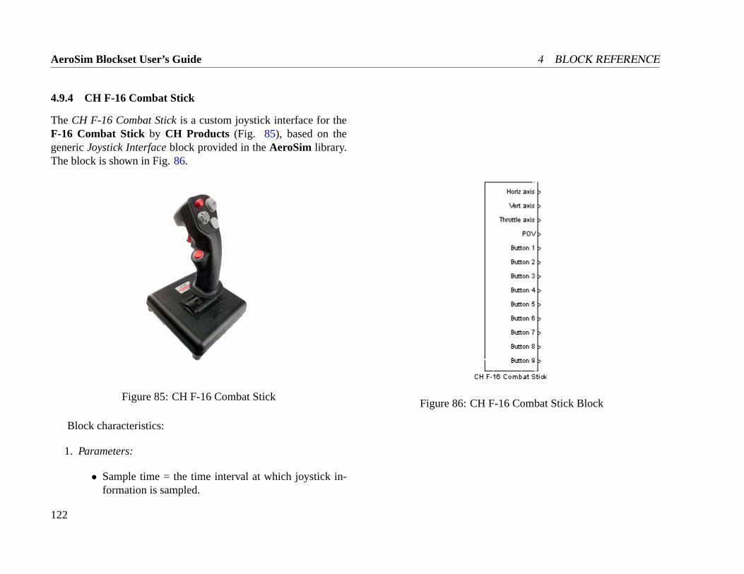
AeroSim Blockset User’s Guide 4 BLOCK REFERENCE
4.9.4 CH F-16 Combat Stick
TheCH F-16 Combat Stickis a custom joystick interface for theF-16 Combat Stick by CH Products (Fig. 85), based on thegenericJoystick Interfaceblock provided in theAeroSim library.The block is shown in Fig.86.
Figure 85: CH F-16 Combat Stick
Block characteristics:
1. Parameters:
• Sample time = the time interval at which joystick in-formation is sampled.
Figure 86: CH F-16 Combat Stick Block
122
4 BLOCK REFERENCE AeroSim Blockset User’s Guide
2. Inputs: no input signals from Simulink, the inputs are pro-vided by the operating system.
3. Outputs:
• Horiz axis = the joystick position on the horizontal axis(0 to 65535).
• Vert axis = the joystick position on the vertical axis (0to 65535).
• Throttle axis = the throttle wheel position (0 to 65535).
• POV = the POV hat position (0=center, 1=up, -1=down,2=right, -2=left).
• Button 1 through 9 = the joystick button states (0=re-leased, 1=pressed).
4. Details: The block is using the same CMEX S-function asthe genericJoystick Interfaceblock, sfunjoy.dll, but it iscustomizing the outputs and providing only those axes andbuttons that are physically available with theF-16 CombatStick device.
5. Usage: The block can be used to provide user inputs forcontrol surfaces deflections, throttle setting and other air-craft commands.
123

AeroSim Blockset User’s Guide 4 BLOCK REFERENCE
4.10 Propulsion
This library folder includes blocks that model various types ofaircraft propulsion systems. Although propulsion models can beextremely complex, the implementations in theAeroSim librarywere kept relatively simple and generic, allowing the designer toquickly develop and test a fully-functional aircraft model.
124
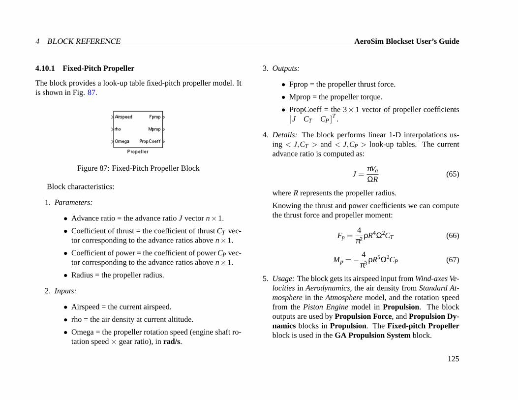
4 BLOCK REFERENCE AeroSim Blockset User’s Guide
4.10.1 Fixed-Pitch Propeller
The block provides a look-up table fixed-pitch propeller model. Itis shown in Fig.87.
Figure 87: Fixed-Pitch Propeller Block
Block characteristics:
1. Parameters:
• Advance ratio = the advance ratioJ vectorn×1.
• Coefficient of thrust = the coefficient of thrustCT vec-tor corresponding to the advance ratios aboven×1.
• Coefficient of power = the coefficient of powerCP vec-tor corresponding to the advance ratios aboven×1.
• Radius = the propeller radius.
2. Inputs:
• Airspeed = the current airspeed.
• rho = the air density at current altitude.
• Omega = the propeller rotation speed (engine shaft ro-tation speed× gear ratio), inrad/s.
3. Outputs:
• Fprop = the propeller thrust force.
• Mprop = the propeller torque.
• PropCoeff = the 3×1 vector of propeller coefficients[J CT CP ]T .
4. Details: The block performs linear 1-D interpolations us-ing < J,CT > and< J,CP > look-up tables. The currentadvance ratio is computed as:
J =πVa
ΩR(65)
whereR represents the propeller radius.
Knowing the thrust and power coefficients we can computethe thrust force and propeller moment:
Fp =4π2ρR4Ω2CT (66)
Mp =− 4π3ρR5Ω2CP (67)
5. Usage:The block gets its airspeed input fromWind-axes Ve-locities in Aerodynamics, the air density fromStandard At-mospherein the Atmospheremodel, and the rotation speedfrom the Piston Enginemodel in Propulsion. The blockoutputs are used byPropulsion Force, andPropulsion Dy-namics blocks inPropulsion. TheFixed-pitch Propellerblock is used in theGA Propulsion Systemblock.
125
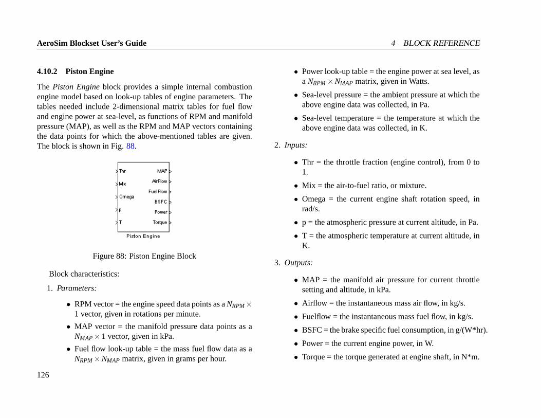
AeroSim Blockset User’s Guide 4 BLOCK REFERENCE
4.10.2 Piston Engine
The Piston Engineblock provides a simple internal combustionengine model based on look-up tables of engine parameters. Thetables needed include 2-dimensional matrix tables for fuel flowand engine power at sea-level, as functions of RPM and manifoldpressure (MAP), as well as the RPM and MAP vectors containingthe data points for which the above-mentioned tables are given.The block is shown in Fig.88.
Figure 88: Piston Engine Block
Block characteristics:
1. Parameters:
• RPM vector = the engine speed data points as aNRPM×1 vector, given in rotations per minute.
• MAP vector = the manifold pressure data points as aNMAP×1 vector, given in kPa.
• Fuel flow look-up table = the mass fuel flow data as aNRPM×NMAP matrix, given in grams per hour.
• Power look-up table = the engine power at sea level, asaNRPM×NMAP matrix, given in Watts.
• Sea-level pressure = the ambient pressure at which theabove engine data was collected, in Pa.
• Sea-level temperature = the temperature at which theabove engine data was collected, in K.
2. Inputs:
• Thr = the throttle fraction (engine control), from 0 to1.
• Mix = the air-to-fuel ratio, or mixture.
• Omega = the current engine shaft rotation speed, inrad/s.
• p = the atmospheric pressure at current altitude, in Pa.
• T = the atmospheric temperature at current altitude, inK.
3. Outputs:
• MAP = the manifold air pressure for current throttlesetting and altitude, in kPa.
• Airflow = the instantaneous mass air flow, in kg/s.
• Fuelflow = the instantaneous mass fuel flow, in kg/s.
• BSFC = the brake specific fuel consumption, in g/(W*hr).
• Power = the current engine power, in W.
• Torque = the torque generated at engine shaft, in N*m.
126
4 BLOCK REFERENCE AeroSim Blockset User’s Guide
4. Details: The throttle input to thisPiston Engineblock repre-sents the fraction between the manifold pressure and atmo-spheric pressure. For normally-aspirated engines, the man-ifold pressure will always be less than or equal to the at-mospheric pressure at current altitude, therefore the pres-sure fraction can take only values from 0 to 1. Practically,the engine runs in a stable manner only for manifold pres-sures of 50-60 kPa and higher. To be able to provide throttlecommand as a throttle actuator position, a look-up table thatmaps pressure ratio to area fraction should be placed aheadof thePiston Engineblock - this mapping is nonlinear and itdepends on the geometry of the intake system.
5. Usage: The Piston Enginesubsystem is used by theGAPropulsion Systemblock.
127
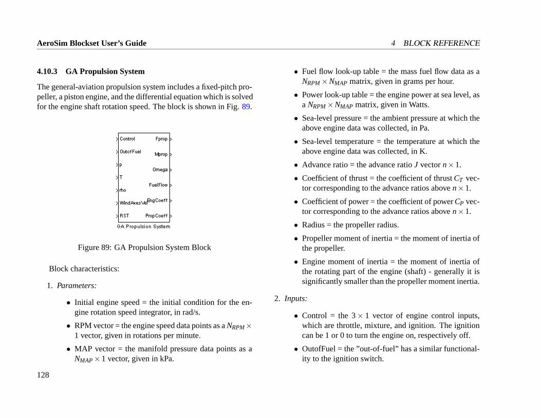
AeroSim Blockset User’s Guide 4 BLOCK REFERENCE
4.10.3 GA Propulsion System
The general-aviation propulsion system includes a fixed-pitch pro-peller, a piston engine, and the differential equation which is solvedfor the engine shaft rotation speed. The block is shown in Fig.89.
Figure 89: GA Propulsion System Block
Block characteristics:
1. Parameters:
• Initial engine speed = the initial condition for the en-gine rotation speed integrator, in rad/s.
• RPM vector = the engine speed data points as aNRPM×1 vector, given in rotations per minute.
• MAP vector = the manifold pressure data points as aNMAP×1 vector, given in kPa.
• Fuel flow look-up table = the mass fuel flow data as aNRPM×NMAP matrix, given in grams per hour.
• Power look-up table = the engine power at sea level, asaNRPM×NMAP matrix, given in Watts.
• Sea-level pressure = the ambient pressure at which theabove engine data was collected, in Pa.
• Sea-level temperature = the temperature at which theabove engine data was collected, in K.
• Advance ratio = the advance ratioJ vectorn×1.
• Coefficient of thrust = the coefficient of thrustCT vec-tor corresponding to the advance ratios aboven×1.
• Coefficient of power = the coefficient of powerCP vec-tor corresponding to the advance ratios aboven×1.
• Radius = the propeller radius.
• Propeller moment of inertia = the moment of inertia ofthe propeller.
• Engine moment of inertia = the moment of inertia ofthe rotating part of the engine (shaft) - generally it issignificantly smaller than the propeller moment inertia.
2. Inputs:
• Control = the 3× 1 vector of engine control inputs,which are throttle, mixture, and ignition. The ignitioncan be 1 or 0 to turn the engine on, respectively off.
• OutofFuel = the ”out-of-fuel” has a similar functional-ity to the ignition switch.
128
4 BLOCK REFERENCE AeroSim Blockset User’s Guide
• p = the atmospheric pressure at current altitude, in Pa.
• T = the atmospheric temperature at current altitude, inK.
• rho = the air density at current altitude.
• WindAxesVel = the 3×1 vector of wind axes velocities(airspeed, sideslip angle, angle-of-attack).
• RST = the engine speed integrator reset flag.
3. Outputs:
• Fprop = the 3×1 vector of propulsion forces (the pro-peller thrust force is on X axis).
• Mprop = the 3×1 vector of propulsion moments (thetorque at engine mount is on X axis).
• Omega = the engine shaft rotation speed, in rad/s.
• Fuelflow = the instantaneous mass fuel flow, in kg/s.
• EngCoeff = the 5×1 vector of engine coefficients, whichinclude MAP, air flow, fuel flow, BSFC, and power.
• PropCoeff = the 3×1 vector of propeller coefficients[J CT CP ]T .
4. Details: TheGA Propulsion Systemincludes aPiston En-gine and aFixed-pitch Propeller. These blocks return thetorque provide by the engine, respectively the torque re-quired by the propeller, at current engine shaft rotation speed,current atmospheric conditions, and airspeed. Then the dif-ferential equation that describes the dynamics of the propul-sion system is:
(Ieng+ Iprop)Ω = Meng+Mprop (68)
This equation is integrated forward in time to compute theengine speedΩ at the next time step.
5. Usage: The GA Propulsion Systemis used in the nonlin-ear aircraft model to compute the propulsion forces and mo-ments that are applied to the vehicle. These will depend onthe engine control inputs, atmospheric conditions, altitude,and airspeed.
129
AeroSim Blockset User’s Guide 4 BLOCK REFERENCE
4.11 Sensors
The Sensorslibrary folder includes generic, analog and digitalsensor models. These can be placed between the aircraft modeland the real or simulated flight control system in order to increasethe realism of the hardware or software in the loop simulation. TheSensors library is divided into 4 sub-folders: noise correlations,generic sensors, analog sensors, and digital sensors.
130
4 BLOCK REFERENCE AeroSim Blockset User’s Guide
4.11.1 Noise Correlation: Random Walk
The block implements a ”Random-Walk” process, by integratingthe output of a white-noise source. The block is pictured in Fig.90.
Figure 90: Random Walk Block
Block characteristics:
1. Parameters:
• White-noise seed = the starting sequence of the white-noise source, for example[23341]. Refer to Math-works documentation on the Simulink block ”White-Noise” for more information about the noise seed.
• Variance = the variance (rms) of the white-noise source.
• Sample time = the sample time of the white-noise source.
2. Inputs:
• None
3. Outputs:
• Output = a random walk noise signal.
4. Details: The random walk process is implemented by inte-grating the output ”w” of a white-noise source:
x = w (69)
5. Usage: The random-walk process is used to simulate thenoise for sensors whose time correlation characteristic is notknown (the random-walk basically assumes infinite correla-tion time).
131
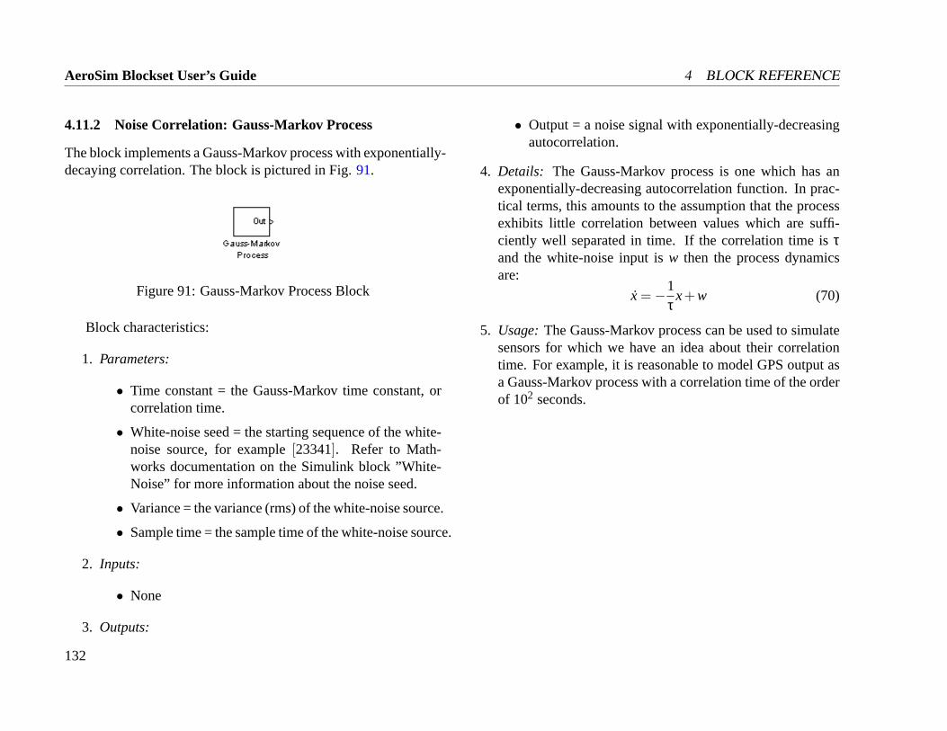
AeroSim Blockset User’s Guide 4 BLOCK REFERENCE
4.11.2 Noise Correlation: Gauss-Markov Process
The block implements a Gauss-Markov process with exponentially-decaying correlation. The block is pictured in Fig.91.
Figure 91: Gauss-Markov Process Block
Block characteristics:
1. Parameters:
• Time constant = the Gauss-Markov time constant, orcorrelation time.
• White-noise seed = the starting sequence of the white-noise source, for example[23341]. Refer to Math-works documentation on the Simulink block ”White-Noise” for more information about the noise seed.
• Variance = the variance (rms) of the white-noise source.
• Sample time = the sample time of the white-noise source.
2. Inputs:
• None
3. Outputs:
• Output = a noise signal with exponentially-decreasingautocorrelation.
4. Details: The Gauss-Markov process is one which has anexponentially-decreasing autocorrelation function. In prac-tical terms, this amounts to the assumption that the processexhibits little correlation between values which are suffi-ciently well separated in time. If the correlation time isτand the white-noise input isw then the process dynamicsare:
x =−1τ
x+w (70)
5. Usage:The Gauss-Markov process can be used to simulatesensors for which we have an idea about their correlationtime. For example, it is reasonable to model GPS output asa Gauss-Markov process with a correlation time of the orderof 102 seconds.
132
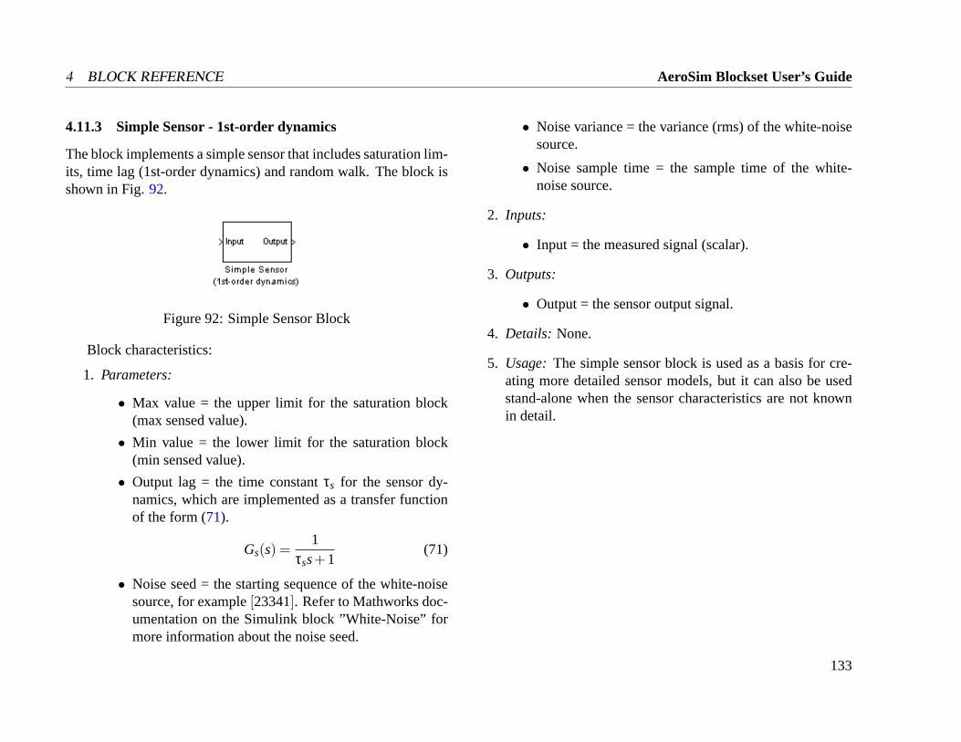
4 BLOCK REFERENCE AeroSim Blockset User’s Guide
4.11.3 Simple Sensor - 1st-order dynamics
The block implements a simple sensor that includes saturation lim-its, time lag (1st-order dynamics) and random walk. The block isshown in Fig.92.
Figure 92: Simple Sensor Block
Block characteristics:
1. Parameters:
• Max value = the upper limit for the saturation block(max sensed value).
• Min value = the lower limit for the saturation block(min sensed value).
• Output lag = the time constantτs for the sensor dy-namics, which are implemented as a transfer functionof the form (71).
Gs(s) =1
τss+1(71)
• Noise seed = the starting sequence of the white-noisesource, for example[23341]. Refer to Mathworks doc-umentation on the Simulink block ”White-Noise” formore information about the noise seed.
• Noise variance = the variance (rms) of the white-noisesource.
• Noise sample time = the sample time of the white-noise source.
2. Inputs:
• Input = the measured signal (scalar).
3. Outputs:
• Output = the sensor output signal.
4. Details: None.
5. Usage: The simple sensor block is used as a basis for cre-ating more detailed sensor models, but it can also be usedstand-alone when the sensor characteristics are not knownin detail.
133
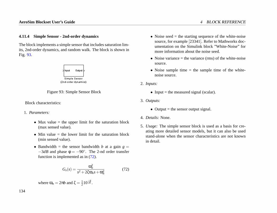
AeroSim Blockset User’s Guide 4 BLOCK REFERENCE
4.11.4 Simple Sensor - 2nd-order dynamics
The block implements a simple sensor that includes saturation lim-its, 2nd-order dynamics, and random walk. The block is shown inFig. 93.
Figure 93: Simple Sensor Block
Block characteristics:
1. Parameters:
• Max value = the upper limit for the saturation block(max sensed value).
• Min value = the lower limit for the saturation block(min sensed value).
• Bandwidth = the sensor bandwidthb at a gaing =−3dB and phaseφ = −90. The 2-nd order transferfunction is implemented as in (72).
Gs(s) =ω2
n
s2 +2ζωns+ω2n
(72)
whereωn = 2πb andζ = 1210
−g20 .
• Noise seed = the starting sequence of the white-noisesource, for example[23341]. Refer to Mathworks doc-umentation on the Simulink block ”White-Noise” formore information about the noise seed.
• Noise variance = the variance (rms) of the white-noisesource.
• Noise sample time = the sample time of the white-noise source.
2. Inputs:
• Input = the measured signal (scalar).
3. Outputs:
• Output = the sensor output signal.
4. Details: None.
5. Usage: The simple sensor block is used as a basis for cre-ating more detailed sensor models, but it can also be usedstand-alone when the sensor characteristics are not knownin detail.
134
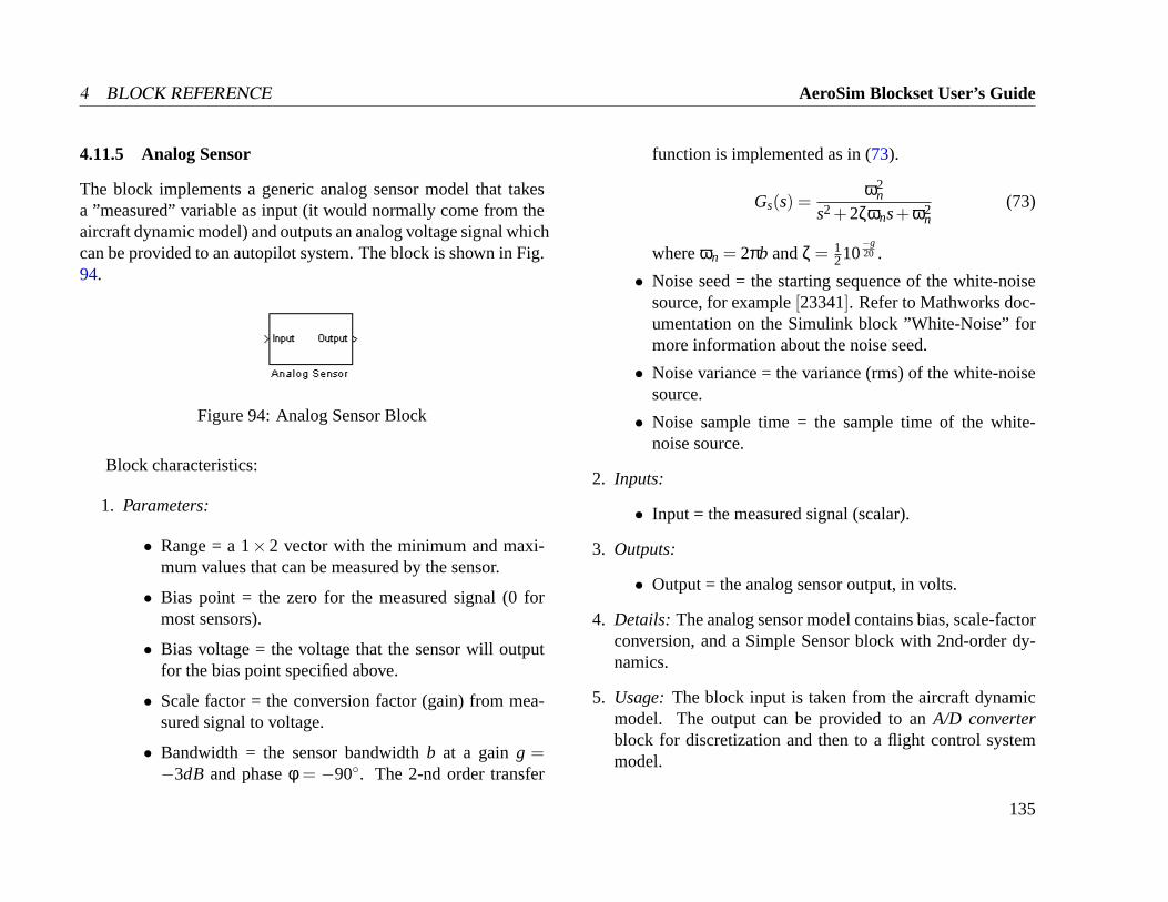
4 BLOCK REFERENCE AeroSim Blockset User’s Guide
4.11.5 Analog Sensor
The block implements a generic analog sensor model that takesa ”measured” variable as input (it would normally come from theaircraft dynamic model) and outputs an analog voltage signal whichcan be provided to an autopilot system. The block is shown in Fig.94.
Figure 94: Analog Sensor Block
Block characteristics:
1. Parameters:
• Range = a 1×2 vector with the minimum and maxi-mum values that can be measured by the sensor.
• Bias point = the zero for the measured signal (0 formost sensors).
• Bias voltage = the voltage that the sensor will outputfor the bias point specified above.
• Scale factor = the conversion factor (gain) from mea-sured signal to voltage.
• Bandwidth = the sensor bandwidthb at a gaing =−3dB and phaseφ = −90. The 2-nd order transfer
function is implemented as in (73).
Gs(s) =ω2
n
s2 +2ζωns+ω2n
(73)
whereωn = 2πb andζ = 1210
−g20 .
• Noise seed = the starting sequence of the white-noisesource, for example[23341]. Refer to Mathworks doc-umentation on the Simulink block ”White-Noise” formore information about the noise seed.
• Noise variance = the variance (rms) of the white-noisesource.
• Noise sample time = the sample time of the white-noise source.
2. Inputs:
• Input = the measured signal (scalar).
3. Outputs:
• Output = the analog sensor output, in volts.
4. Details: The analog sensor model contains bias, scale-factorconversion, and a Simple Sensor block with 2nd-order dy-namics.
5. Usage: The block input is taken from the aircraft dynamicmodel. The output can be provided to anA/D converterblock for discretization and then to a flight control systemmodel.
135
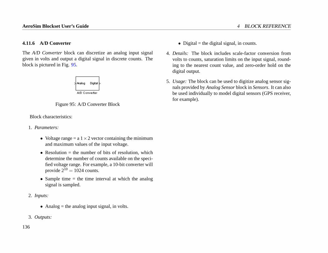
AeroSim Blockset User’s Guide 4 BLOCK REFERENCE
4.11.6 A/D Converter
The A/D Converterblock can discretize an analog input signalgiven in volts and output a digital signal in discrete counts. Theblock is pictured in Fig.95.
Figure 95: A/D Converter Block
Block characteristics:
1. Parameters:
• Voltage range = a 1×2 vector containing the minimumand maximum values of the input voltage.
• Resolution = the number of bits of resolution, whichdetermine the number of counts available on the speci-fied voltage range. For example, a 10-bit converter willprovide 210 = 1024 counts.
• Sample time = the time interval at which the analogsignal is sampled.
2. Inputs:
• Analog = the analog input signal, in volts.
3. Outputs:
• Digital = the digital signal, in counts.
4. Details: The block includes scale-factor conversion fromvolts to counts, saturation limits on the input signal, round-ing to the nearest count value, and zero-order hold on thedigital output.
5. Usage:The block can be used to digitize analog sensor sig-nals provided byAnalog Sensorblock inSensors. It can alsobe used individually to model digital sensors (GPS receiver,for example).
136
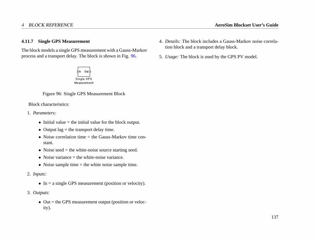
4 BLOCK REFERENCE AeroSim Blockset User’s Guide
4.11.7 Single GPS Measurement
The block models a single GPS measurement with a Gauss-Markovprocess and a transport delay. The block is shown in Fig.96.
Figure 96: Single GPS Measurement Block
Block characteristics:
1. Parameters:
• Initial value = the initial value for the block output.
• Output lag = the transport delay time.
• Noise correlation time = the Gauss-Markov time con-stant.
• Noise seed = the white-noise source starting seed.
• Noise variance = the white-noise variance.
• Noise sample time = the white noise sample time.
2. Inputs:
• In = a single GPS measurement (position or velocity).
3. Outputs:
• Out = the GPS measurement output (position or veloc-ity).
4. Details: The block includes a Gauss-Markov noise correla-tion block and a transport delay block.
5. Usage:The block is used by the GPS PV model.
137
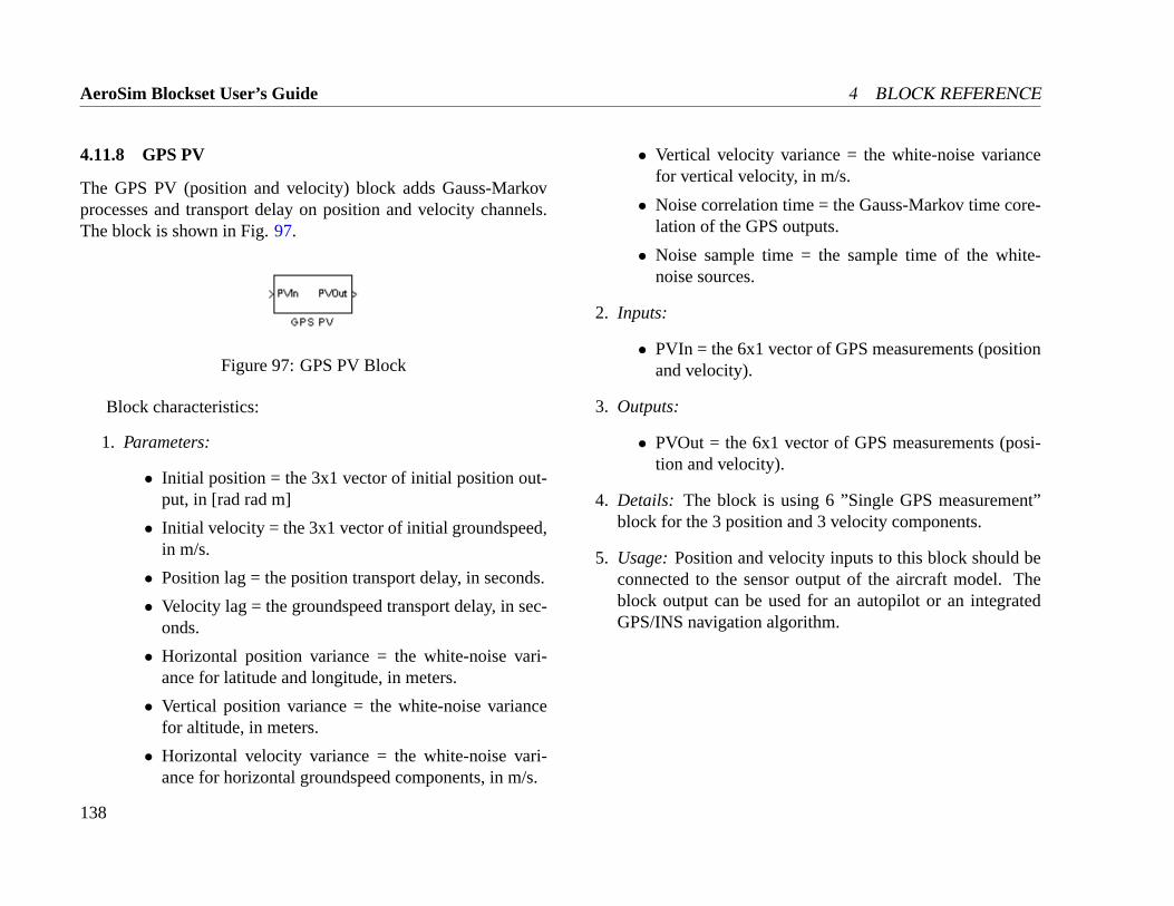
AeroSim Blockset User’s Guide 4 BLOCK REFERENCE
4.11.8 GPS PV
The GPS PV (position and velocity) block adds Gauss-Markovprocesses and transport delay on position and velocity channels.The block is shown in Fig.97.
Figure 97: GPS PV Block
Block characteristics:
1. Parameters:
• Initial position = the 3x1 vector of initial position out-put, in [rad rad m]
• Initial velocity = the 3x1 vector of initial groundspeed,in m/s.
• Position lag = the position transport delay, in seconds.
• Velocity lag = the groundspeed transport delay, in sec-onds.
• Horizontal position variance = the white-noise vari-ance for latitude and longitude, in meters.
• Vertical position variance = the white-noise variancefor altitude, in meters.
• Horizontal velocity variance = the white-noise vari-ance for horizontal groundspeed components, in m/s.
• Vertical velocity variance = the white-noise variancefor vertical velocity, in m/s.
• Noise correlation time = the Gauss-Markov time core-lation of the GPS outputs.
• Noise sample time = the sample time of the white-noise sources.
2. Inputs:
• PVIn = the 6x1 vector of GPS measurements (positionand velocity).
3. Outputs:
• PVOut = the 6x1 vector of GPS measurements (posi-tion and velocity).
4. Details: The block is using 6 ”Single GPS measurement”block for the 3 position and 3 velocity components.
5. Usage:Position and velocity inputs to this block should beconnected to the sensor output of the aircraft model. Theblock output can be used for an autopilot or an integratedGPS/INS navigation algorithm.
138
4 BLOCK REFERENCE AeroSim Blockset User’s Guide
4.12 Transformations
TheTransformations library folder includes parameter and refer-ence frame transformations that are required in the aircraft modelequations or in autopilot design.
139
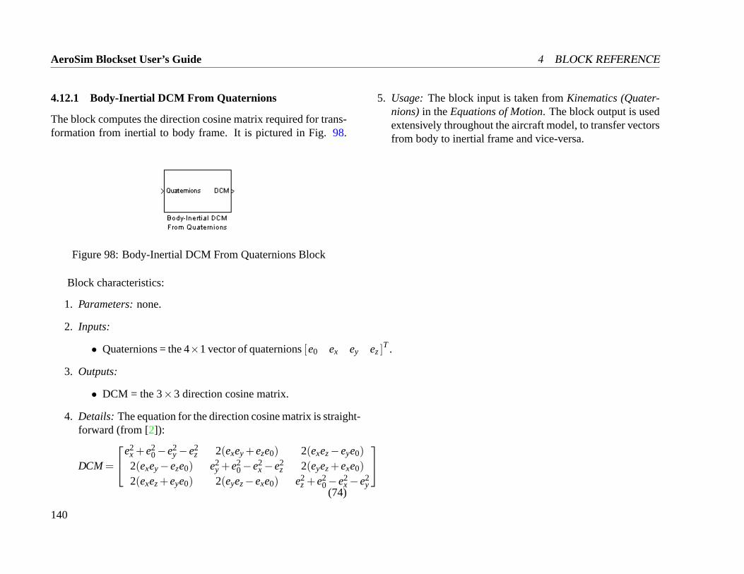
AeroSim Blockset User’s Guide 4 BLOCK REFERENCE
4.12.1 Body-Inertial DCM From Quaternions
The block computes the direction cosine matrix required for trans-formation from inertial to body frame. It is pictured in Fig.98.
Figure 98: Body-Inertial DCM From Quaternions Block
Block characteristics:
1. Parameters:none.
2. Inputs:
• Quaternions = the 4×1 vector of quaternions[e0 ex ey ez]T .
3. Outputs:
• DCM = the 3×3 direction cosine matrix.
4. Details: The equation for the direction cosine matrix is straight-forward (from [2]):
DCM=
e2x +e2
0−e2y−e2
z 2(exey +eze0) 2(exez−eye0)2(exey−eze0) e2
y +e20−e2
x−e2z 2(eyez+exe0)
2(exez+eye0) 2(eyez−exe0) e2z +e2
0−e2x−e2
y
(74)
5. Usage:The block input is taken fromKinematics (Quater-nions)in theEquations of Motion. The block output is usedextensively throughout the aircraft model, to transfer vectorsfrom body to inertial frame and vice-versa.
140
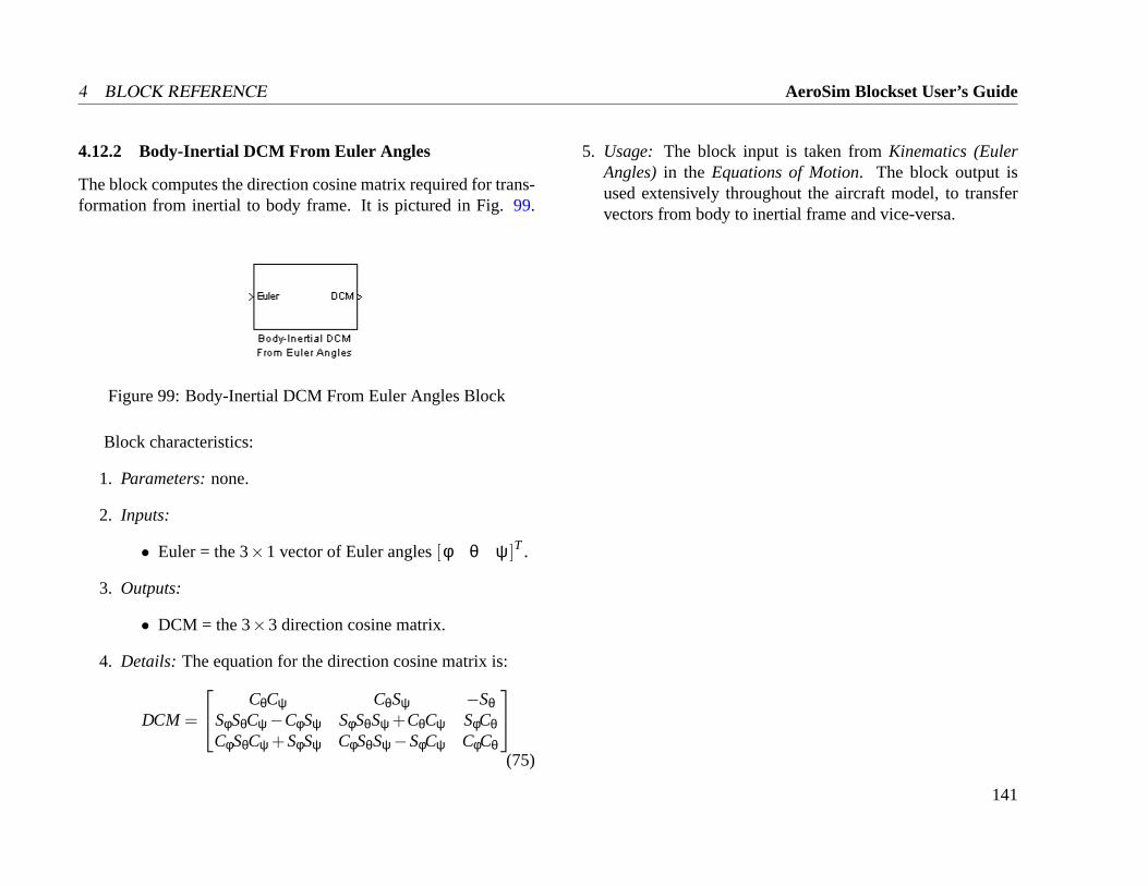
4 BLOCK REFERENCE AeroSim Blockset User’s Guide
4.12.2 Body-Inertial DCM From Euler Angles
The block computes the direction cosine matrix required for trans-formation from inertial to body frame. It is pictured in Fig.99.
Figure 99: Body-Inertial DCM From Euler Angles Block
Block characteristics:
1. Parameters:none.
2. Inputs:
• Euler = the 3×1 vector of Euler angles[φ θ ψ ]T .
3. Outputs:
• DCM = the 3×3 direction cosine matrix.
4. Details: The equation for the direction cosine matrix is:
DCM =
CθCψ CθSψ −SθSφSθCψ−CφSψ SφSθSψ +CθCψ SφCθCφSθCψ +SφSψ CφSθSψ−SφCψ CφCθ
(75)
5. Usage: The block input is taken fromKinematics (EulerAngles)in the Equations of Motion. The block output isused extensively throughout the aircraft model, to transfervectors from body to inertial frame and vice-versa.
141
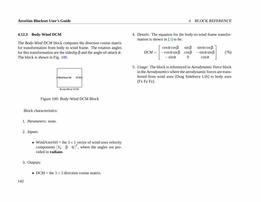
AeroSim Blockset User’s Guide 4 BLOCK REFERENCE
4.12.3 Body-Wind DCM
TheBody-Wind DCMblock computes the direction cosine matrixfor transformation from body to wind frame. The rotation anglesfor this transformation are the sideslipβ and the angle-of-attackα.The block is shown in Fig.100.
Figure 100: Body-Wind DCM Block
Block characteristics:
1. Parameters:none.
2. Inputs:
• WindAxesVel = the 3×1 vector of wind-axes velocitycomponents[Va β α ]T , where the angles are pro-vided inradians.
3. Outputs:
• DCM = the 3×3 direction cosine matrix.
4. Details: The equation for the body-to-wind frame transfor-mation is shown in [3] to be:
DCM =
cosαcosβ sinβ sinαcosβ−cosαsinβ cosβ −sinαsinβ−sinα 0 cosα
(76)
5. Usage:The block is referenced inAerodynamic Forceblockin theAerodynamicswhere the aerodynamic forces are trans-ferred from wind axes [Drag Sideforce Lift] to body axes[Fx Fy Fz].
142
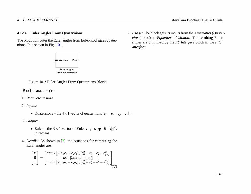
4 BLOCK REFERENCE AeroSim Blockset User’s Guide
4.12.4 Euler Angles From Quaternions
The block computes the Euler angles from Euler-Rodrigues quater-nions. It is shown in Fig.101.
Figure 101: Euler Angles From Quaternions Block
Block characteristics:
1. Parameters:none.
2. Inputs:
• Quaternions = the 4×1 vector of quaternions[e0 ex ey ez]T .
3. Outputs:
• Euler = the 3×1 vector of Euler angles[φ θ ψ ]T ,in radians.
4. Details: As shown in [2], the equations for computing theEuler angles are: φ
θψ
=
atan2[2(e0ex +eyez),(e2
0 +e2z−e2
x−e2y)]
asin[2(e0ey−exez)]atan2
[2(e0ez+exey),(e2
0 +e2x−e2
y−e2z)](77)
5. Usage:The block gets its inputs from theKinematics (Quater-nions) block in Equations of Motion. The resulting Eulerangles are only used by theFS Interfaceblock in thePilotInterface.
143
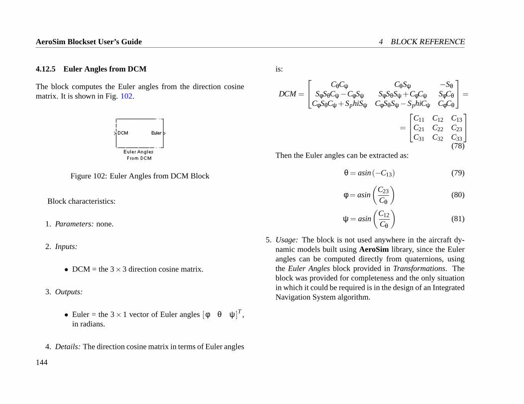
AeroSim Blockset User’s Guide 4 BLOCK REFERENCE
4.12.5 Euler Angles from DCM
The block computes the Euler angles from the direction cosinematrix. It is shown in Fig.102.
Figure 102: Euler Angles from DCM Block
Block characteristics:
1. Parameters:none.
2. Inputs:
• DCM = the 3×3 direction cosine matrix.
3. Outputs:
• Euler = the 3×1 vector of Euler angles[φ θ ψ ]T ,in radians.
4. Details: The direction cosine matrix in terms of Euler angles
is:
DCM =
CθCψ CθSψ −SθSφSθCψ−CφSψ SφSθSψ +CφCψ SφCθ
CφSθCψ +SphiSψ CφSθSψ−SphiCψ CφCθ
=
=
C11 C12 C13
C21 C22 C23
C31 C32 C33
(78)
Then the Euler angles can be extracted as:
θ = asin(−C13) (79)
φ = asin
(C23
Cθ
)(80)
ψ = asin
(C12
Cθ
)(81)
5. Usage: The block is not used anywhere in the aircraft dy-namic models built usingAeroSim library, since the Eulerangles can be computed directly from quaternions, usingthe Euler Anglesblock provided inTransformations. Theblock was provided for completeness and the only situationin which it could be required is in the design of an IntegratedNavigation System algorithm.
144
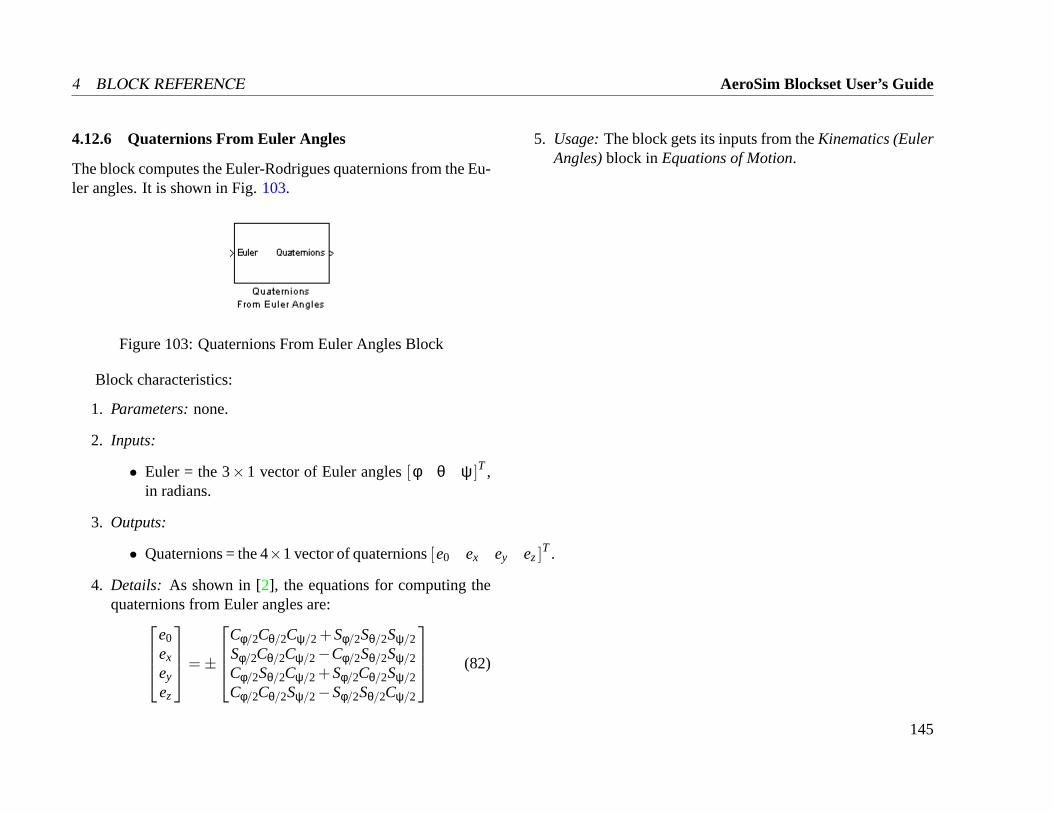
4 BLOCK REFERENCE AeroSim Blockset User’s Guide
4.12.6 Quaternions From Euler Angles
The block computes the Euler-Rodrigues quaternions from the Eu-ler angles. It is shown in Fig.103.
Figure 103: Quaternions From Euler Angles Block
Block characteristics:
1. Parameters:none.
2. Inputs:
• Euler = the 3×1 vector of Euler angles[φ θ ψ ]T ,in radians.
3. Outputs:
• Quaternions = the 4×1 vector of quaternions[e0 ex ey ez]T .
4. Details: As shown in [2], the equations for computing thequaternions from Euler angles are:
e0
ex
ey
ez
=±
Cφ/2Cθ/2Cψ/2 +Sφ/2Sθ/2Sψ/2Sφ/2Cθ/2Cψ/2−Cφ/2Sθ/2Sψ/2Cφ/2Sθ/2Cψ/2 +Sφ/2Cθ/2Sψ/2Cφ/2Cθ/2Sψ/2−Sφ/2Sθ/2Cψ/2
(82)
5. Usage:The block gets its inputs from theKinematics (EulerAngles)block inEquations of Motion.
145
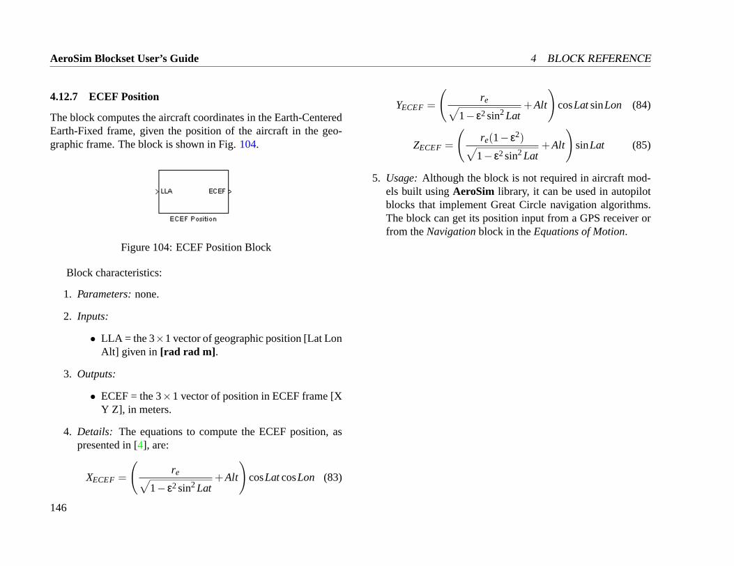
AeroSim Blockset User’s Guide 4 BLOCK REFERENCE
4.12.7 ECEF Position
The block computes the aircraft coordinates in the Earth-CenteredEarth-Fixed frame, given the position of the aircraft in the geo-graphic frame. The block is shown in Fig.104.
Figure 104: ECEF Position Block
Block characteristics:
1. Parameters:none.
2. Inputs:
• LLA = the 3×1 vector of geographic position [Lat LonAlt] given in [rad rad m] .
3. Outputs:
• ECEF = the 3×1 vector of position in ECEF frame [XY Z], in meters.
4. Details: The equations to compute the ECEF position, aspresented in [4], are:
XECEF =
(re√
1− ε2sin2Lat+Alt
)cosLatcosLon (83)
YECEF =
(re√
1− ε2sin2Lat+Alt
)cosLatsinLon (84)
ZECEF =
(re(1− ε2)√
1− ε2sin2Lat+Alt
)sinLat (85)
5. Usage:Although the block is not required in aircraft mod-els built usingAeroSim library, it can be used in autopilotblocks that implement Great Circle navigation algorithms.The block can get its position input from a GPS receiver orfrom theNavigationblock in theEquations of Motion.
146
4 BLOCK REFERENCE AeroSim Blockset User’s Guide
4.13 Unit Conversion
For consistency with various look-up table models provided in theAeroSim library we recommend the use of radians for angular po-sitions, velocities, and accelerations, and the use of metric unitsfor everything else. TheUnit Conversion blocks were providedfor cases when degrees for angles and/or English units for otherparameters are required in the aircraft model. In this cases we rec-ommend placing the unit conversion blocks on the inputs and out-puts of the aircraft model, such that, internally, the aircraft modelstill operates in metric units but the model inputs and outputs areprovided in the units of choice.
147

AeroSim Blockset User’s Guide 4 BLOCK REFERENCE
4.13.1 Angular position: Deg 2 rad and Rad 2 deg
The blocks convert angle inputs from degrees to radians and vice-versa. They are shown in Fig.105.
Figure 105: Deg 2 rad and Rad 2 deg Blocks
Block characteristics:
1. Parameters:none.
2. Inputs:
• In = angle in degrees, respectively radians.
3. Outputs:
• Out = angle in radians, respectively degrees.
4. Details: The conversion factor from degrees to radians isπ/180.
5. Usage: All angle inputs for theAeroSim library blocksshould be given in radians. The blocks can be used by thedesigner to provide aircraft model inputs/outputs in degrees.
148
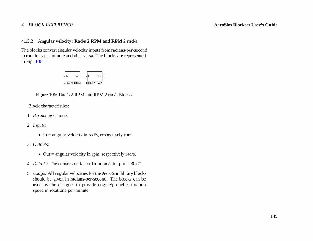
4 BLOCK REFERENCE AeroSim Blockset User’s Guide
4.13.2 Angular velocity: Rad/s 2 RPM and RPM 2 rad/s
The blocks convert angular velocity inputs from radians-per-secondto rotations-per-minute and vice-versa. The blocks are representedin Fig. 106.
Figure 106: Rad/s 2 RPM and RPM 2 rad/s Blocks
Block characteristics:
1. Parameters:none.
2. Inputs:
• In = angular velocity in rad/s, respectively rpm.
3. Outputs:
• Out = angular velocity in rpm, respectively rad/s.
4. Details: The conversion factor from rad/s to rpm is 30/π.
5. Usage:All angular velocities for theAeroSim library blocksshould be given in radians-per-second. The blocks can beused by the designer to provide engine/propeller rotationspeed in rotations-per-minute.
149
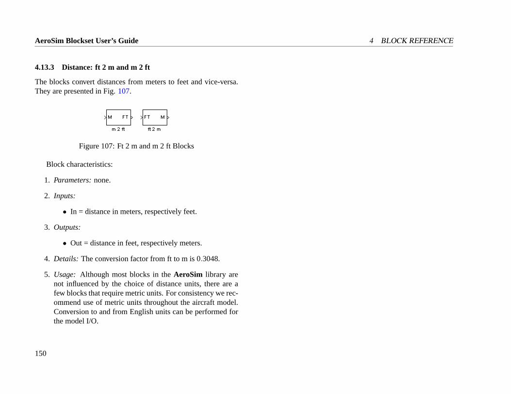
AeroSim Blockset User’s Guide 4 BLOCK REFERENCE
4.13.3 Distance: ft 2 m and m 2 ft
The blocks convert distances from meters to feet and vice-versa.They are presented in Fig.107.
Figure 107: Ft 2 m and m 2 ft Blocks
Block characteristics:
1. Parameters:none.
2. Inputs:
• In = distance in meters, respectively feet.
3. Outputs:
• Out = distance in feet, respectively meters.
4. Details: The conversion factor from ft to m is 0.3048.
5. Usage: Although most blocks in theAeroSim library arenot influenced by the choice of distance units, there are afew blocks that require metric units. For consistency we rec-ommend use of metric units throughout the aircraft model.Conversion to and from English units can be performed forthe model I/O.
150
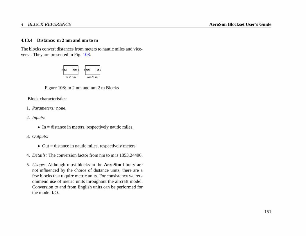
4 BLOCK REFERENCE AeroSim Blockset User’s Guide
4.13.4 Distance: m 2 nm and nm to m
The blocks convert distances from meters to nautic miles and vice-versa. They are presented in Fig.108.
Figure 108: m 2 nm and nm 2 m Blocks
Block characteristics:
1. Parameters:none.
2. Inputs:
• In = distance in meters, respectively nautic miles.
3. Outputs:
• Out = distance in nautic miles, respectively meters.
4. Details: The conversion factor from nm to m is 1853.24496.
5. Usage: Although most blocks in theAeroSim library arenot influenced by the choice of distance units, there are afew blocks that require metric units. For consistency we rec-ommend use of metric units throughout the aircraft model.Conversion to and from English units can be performed forthe model I/O.
151
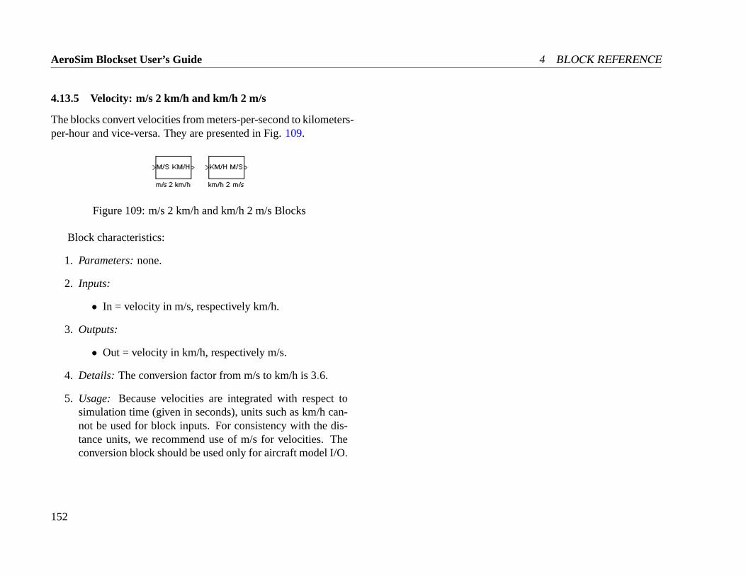
AeroSim Blockset User’s Guide 4 BLOCK REFERENCE
4.13.5 Velocity: m/s 2 km/h and km/h 2 m/s
The blocks convert velocities from meters-per-second to kilometers-per-hour and vice-versa. They are presented in Fig.109.
Figure 109: m/s 2 km/h and km/h 2 m/s Blocks
Block characteristics:
1. Parameters:none.
2. Inputs:
• In = velocity in m/s, respectively km/h.
3. Outputs:
• Out = velocity in km/h, respectively m/s.
4. Details: The conversion factor from m/s to km/h is 3.6.
5. Usage: Because velocities are integrated with respect tosimulation time (given in seconds), units such as km/h can-not be used for block inputs. For consistency with the dis-tance units, we recommend use of m/s for velocities. Theconversion block should be used only for aircraft model I/O.
152
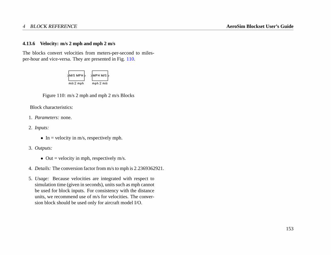
4 BLOCK REFERENCE AeroSim Blockset User’s Guide
4.13.6 Velocity: m/s 2 mph and mph 2 m/s
The blocks convert velocities from meters-per-second to miles-per-hour and vice-versa. They are presented in Fig.110.
Figure 110: m/s 2 mph and mph 2 m/s Blocks
Block characteristics:
1. Parameters:none.
2. Inputs:
• In = velocity in m/s, respectively mph.
3. Outputs:
• Out = velocity in mph, respectively m/s.
4. Details: The conversion factor from m/s to mph is 2.2369362921.
5. Usage: Because velocities are integrated with respect tosimulation time (given in seconds), units such as mph cannotbe used for block inputs. For consistency with the distanceunits, we recommend use of m/s for velocities. The conver-sion block should be used only for aircraft model I/O.
153
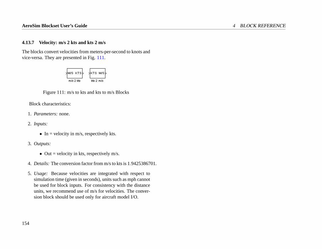
AeroSim Blockset User’s Guide 4 BLOCK REFERENCE
4.13.7 Velocity: m/s 2 kts and kts 2 m/s
The blocks convert velocities from meters-per-second to knots andvice-versa. They are presented in Fig.111.
Figure 111: m/s to kts and kts to m/s Blocks
Block characteristics:
1. Parameters:none.
2. Inputs:
• In = velocity in m/s, respectively kts.
3. Outputs:
• Out = velocity in kts, respectively m/s.
4. Details: The conversion factor from m/s to kts is 1.9425386701.
5. Usage: Because velocities are integrated with respect tosimulation time (given in seconds), units such as mph cannotbe used for block inputs. For consistency with the distanceunits, we recommend use of m/s for velocities. The conver-sion block should be used only for aircraft model I/O.
154
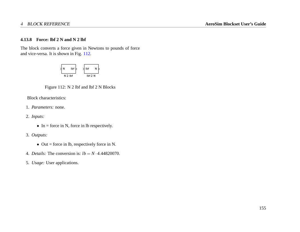
4 BLOCK REFERENCE AeroSim Blockset User’s Guide
4.13.8 Force: lbf 2 N and N 2 lbf
The block converts a force given in Newtons to pounds of forceand vice-versa. It is shown in Fig.112.
Figure 112: N 2 lbf and lbf 2 N Blocks
Block characteristics:
1. Parameters:none.
2. Inputs:
• In = force in N, force in lb respectively.
3. Outputs:
• Out = force in lb, respectively force in N.
4. Details: The conversion is:lb = N ·4.44820070.
5. Usage:User applications.
155
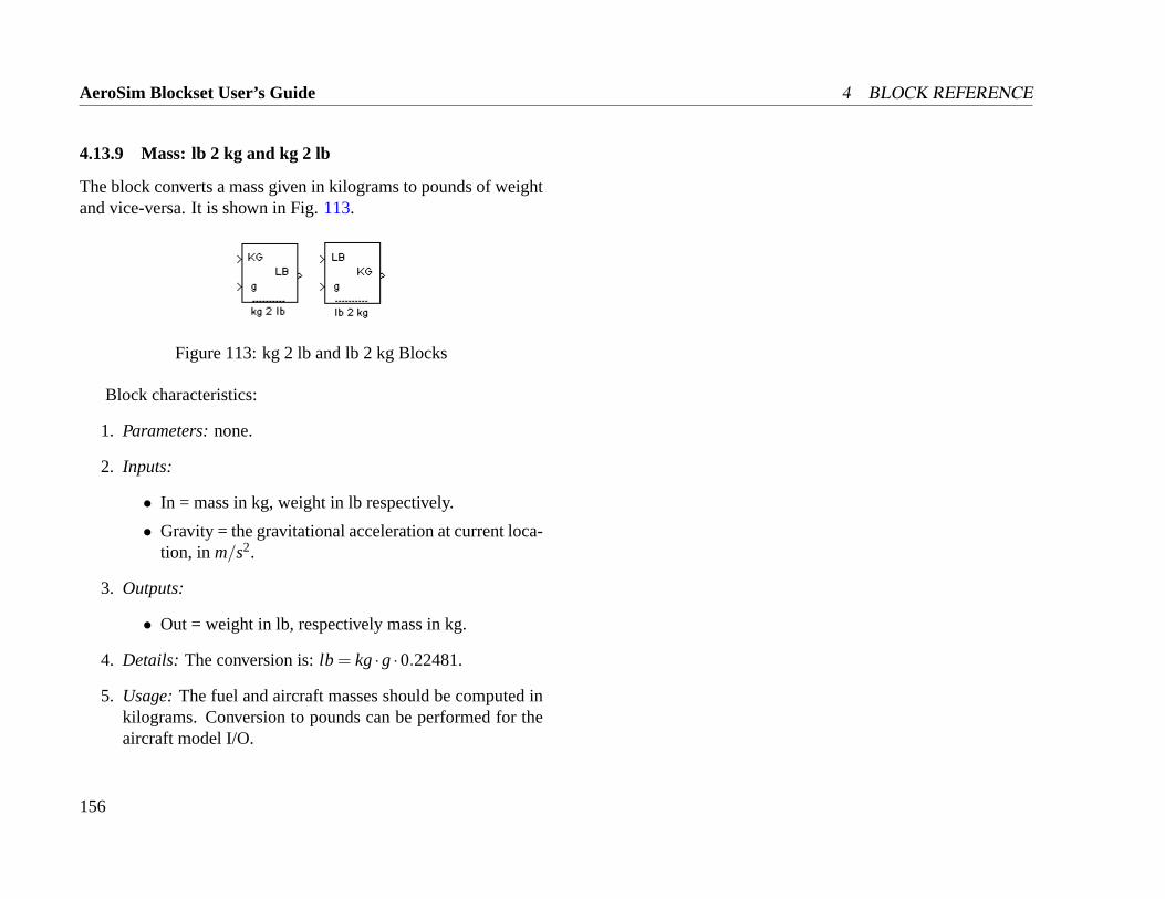
AeroSim Blockset User’s Guide 4 BLOCK REFERENCE
4.13.9 Mass: lb 2 kg and kg 2 lb
The block converts a mass given in kilograms to pounds of weightand vice-versa. It is shown in Fig.113.
Figure 113: kg 2 lb and lb 2 kg Blocks
Block characteristics:
1. Parameters:none.
2. Inputs:
• In = mass in kg, weight in lb respectively.
• Gravity = the gravitational acceleration at current loca-tion, in m/s2.
3. Outputs:
• Out = weight in lb, respectively mass in kg.
4. Details: The conversion is:lb = kg·g·0.22481.
5. Usage:The fuel and aircraft masses should be computed inkilograms. Conversion to pounds can be performed for theaircraft model I/O.
156
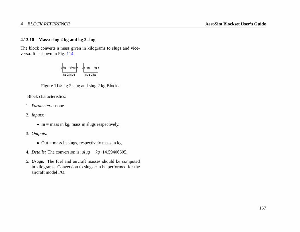
4 BLOCK REFERENCE AeroSim Blockset User’s Guide
4.13.10 Mass: slug 2 kg and kg 2 slug
The block converts a mass given in kilograms to slugs and vice-versa. It is shown in Fig.114.
Figure 114: kg 2 slug and slug 2 kg Blocks
Block characteristics:
1. Parameters:none.
2. Inputs:
• In = mass in kg, mass in slugs respectively.
3. Outputs:
• Out = mass in slugs, respectively mass in kg.
4. Details: The conversion is:slug= kg·14.59406605.
5. Usage: The fuel and aircraft masses should be computedin kilograms. Conversion to slugs can be performed for theaircraft model I/O.
157
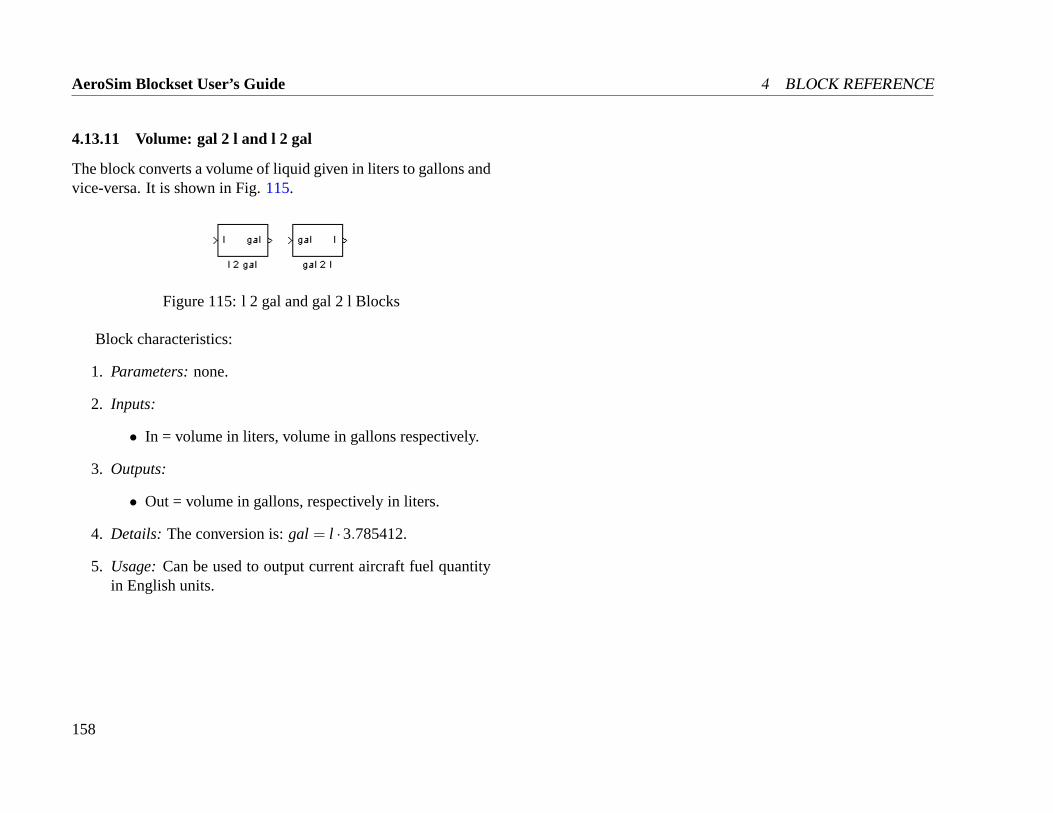
AeroSim Blockset User’s Guide 4 BLOCK REFERENCE
4.13.11 Volume: gal 2 l and l 2 gal
The block converts a volume of liquid given in liters to gallons andvice-versa. It is shown in Fig.115.
Figure 115: l 2 gal and gal 2 l Blocks
Block characteristics:
1. Parameters:none.
2. Inputs:
• In = volume in liters, volume in gallons respectively.
3. Outputs:
• Out = volume in gallons, respectively in liters.
4. Details: The conversion is:gal = l ·3.785412.
5. Usage:Can be used to output current aircraft fuel quantityin English units.
158
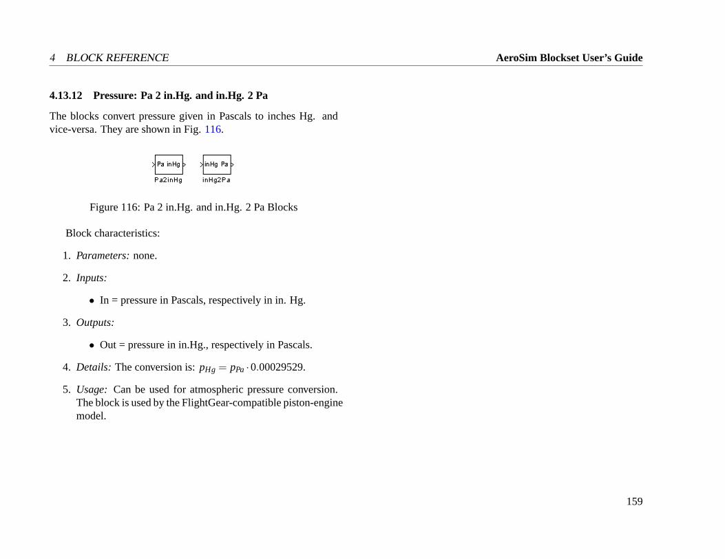
4 BLOCK REFERENCE AeroSim Blockset User’s Guide
4.13.12 Pressure: Pa 2 in.Hg. and in.Hg. 2 Pa
The blocks convert pressure given in Pascals to inches Hg. andvice-versa. They are shown in Fig.116.
Figure 116: Pa 2 in.Hg. and in.Hg. 2 Pa Blocks
Block characteristics:
1. Parameters:none.
2. Inputs:
• In = pressure in Pascals, respectively in in. Hg.
3. Outputs:
• Out = pressure in in.Hg., respectively in Pascals.
4. Details: The conversion is:pHg = pPa ·0.00029529.
5. Usage: Can be used for atmospheric pressure conversion.The block is used by the FlightGear-compatible piston-enginemodel.
159
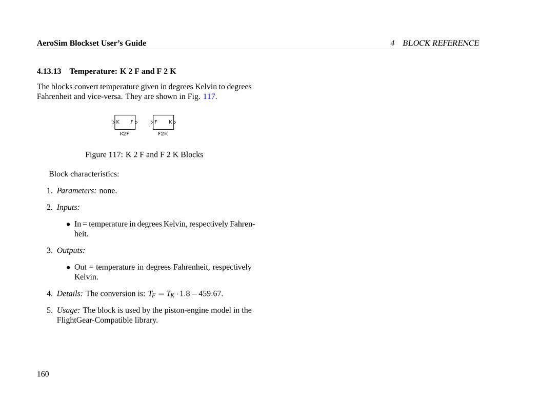
AeroSim Blockset User’s Guide 4 BLOCK REFERENCE
4.13.13 Temperature: K 2 F and F 2 K
The blocks convert temperature given in degrees Kelvin to degreesFahrenheit and vice-versa. They are shown in Fig.117.
Figure 117: K 2 F and F 2 K Blocks
Block characteristics:
1. Parameters:none.
2. Inputs:
• In = temperature in degrees Kelvin, respectively Fahren-heit.
3. Outputs:
• Out = temperature in degrees Fahrenheit, respectivelyKelvin.
4. Details: The conversion is:TF = TK ·1.8−459.67.
5. Usage:The block is used by the piston-engine model in theFlightGear-Compatible library.
160
4 BLOCK REFERENCE AeroSim Blockset User’s Guide
4.14 FlightGear-Compatible
AeroSim’s FlightGear-compatibility layer includes XML parsersthat can load aircraft, engine, and thruster parameters into Mat-lab structures, as well as the necessary aircraft-dynamics blocksthat use such Matlab structures. These aircraft dynamics blocksas well as several complete aircraft models can be found in theFlightGear-Compatible library folder and they are presented indetail in this subsection.
161
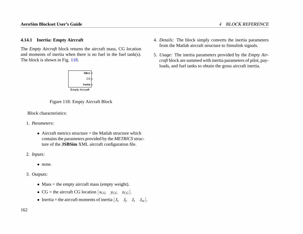
AeroSim Blockset User’s Guide 4 BLOCK REFERENCE
4.14.1 Inertia: Empty Aircraft
The Empty Aircraftblock returns the aircraft mass, CG locationand moments of inertia when there is no fuel in the fuel tank(s).The block is shown in Fig.118.
Figure 118: Empty Aircraft Block
Block characteristics:
1. Parameters:
• Aircraft metrics structure = the Matlab structure whichcontains the parameters provided by theMETRICSstruc-ture of theJSBSimXML aircraft configuration file.
2. Inputs:
• none.
3. Outputs:
• Mass = the empty aircraft mass (empty weight).
• CG = the aircraft CG location[xCG yCG zCG].
• Inertia = the aircraft moments of inertia[Jx Jy Jz Jxz].
4. Details: The block simply converts the inertia parametersfrom the Matlab aircraft structure to Simulink signals.
5. Usage: The inertia parameters provided by theEmpty Air-craft block are summed with inertia parameters of pilot, pay-loads, and fuel tanks to obtain the gross aircraft inertia.
162
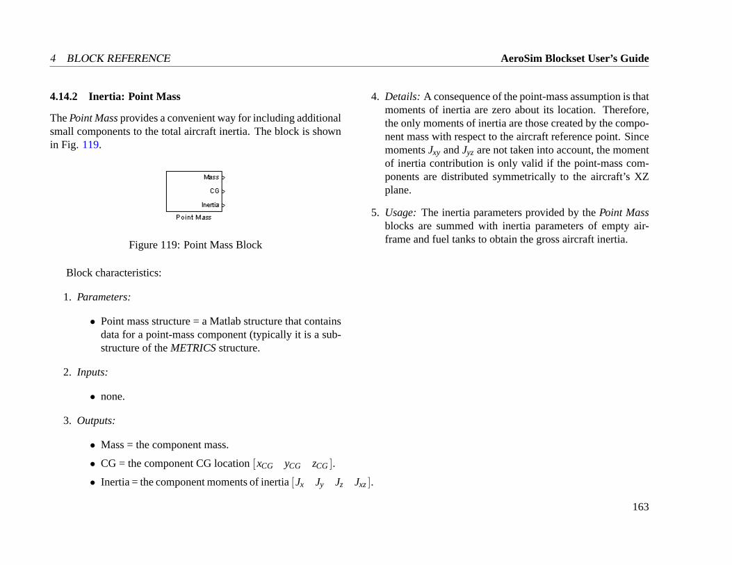
4 BLOCK REFERENCE AeroSim Blockset User’s Guide
4.14.2 Inertia: Point Mass
ThePoint Massprovides a convenient way for including additionalsmall components to the total aircraft inertia. The block is shownin Fig. 119.
Figure 119: Point Mass Block
Block characteristics:
1. Parameters:
• Point mass structure = a Matlab structure that containsdata for a point-mass component (typically it is a sub-structure of theMETRICSstructure.
2. Inputs:
• none.
3. Outputs:
• Mass = the component mass.
• CG = the component CG location[xCG yCG zCG].
• Inertia = the component moments of inertia[Jx Jy Jz Jxz].
4. Details: A consequence of the point-mass assumption is thatmoments of inertia are zero about its location. Therefore,the only moments of inertia are those created by the compo-nent mass with respect to the aircraft reference point. SincemomentsJxy andJyz are not taken into account, the momentof inertia contribution is only valid if the point-mass com-ponents are distributed symmetrically to the aircraft’s XZplane.
5. Usage: The inertia parameters provided by thePoint Massblocks are summed with inertia parameters of empty air-frame and fuel tanks to obtain the gross aircraft inertia.
163
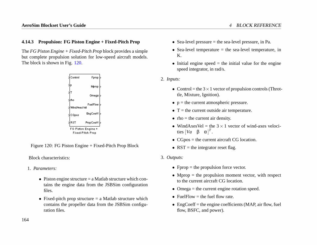
AeroSim Blockset User’s Guide 4 BLOCK REFERENCE
4.14.3 Propulsion: FG Piston Engine + Fixed-Pitch Prop
TheFG Piston Engine + Fixed-Pitch Propblock provides a simplebut complete propulsion solution for low-speed aircraft models.The block is shown in Fig.120.
Figure 120: FG Piston Engine + Fixed-Pitch Prop Block
Block characteristics:
1. Parameters:
• Piston engine structure = a Matlab structure which con-tains the engine data from the JSBSim configurationfiles.
• Fixed-pitch prop structure = a Matlab structure whichcontains the propeller data from the JSBSim configu-ration files.
• Sea-level pressure = the sea-level pressure, in Pa.
• Sea-level temperature = the sea-level temperature, inK.
• Initial engine speed = the initial value for the enginespeed integrator, in rad/s.
2. Inputs:
• Control = the 3×1 vector of propulsion controls (Throt-tle, Mixture, Ignition).
• p = the current atmospheric pressure.
• T = the current outside air temperature.
• rho = the current air density.
• WindAxesVel = the 3×1 vector of wind-axes veloci-ties[Va β α ]T .
• CGpos = the current aircraft CG location.
• RST = the integrator reset flag.
3. Outputs:
• Fprop = the propulsion force vector.
• Mprop = the propulsion moment vector, with respectto the current aircraft CG location.
• Omega = the current engine rotation speed.
• FuelFlow = the fuel flow rate.
• EngCoeff = the engine coefficients (MAP, air flow, fuelflow, BSFC, and power).
164
4 BLOCK REFERENCE AeroSim Blockset User’s Guide
• PropCoeff = the propeller coefficients (advance ratio,thrust coefficient, and power coefficient).
4. Details: The block includes links to theFG Piston Engineand to theFG Fixed-Pitch Propellerblocks which can befound in theAeroSim library. The block integrates the an-gular acceleration obtained from the difference between theavailable engine torque and the required propeller torque,by dividing it by the moment of inertia of the rotating com-ponents. Typically the moment of the inertia of the engineshaft is small compared to the propeller moment of inertia,so it can be ignored.
5. Usage:The block is used to model a single propulsion unitand its resulting forces and moments. Multi-engine aircraftwill use multiple blocks of this type.
165
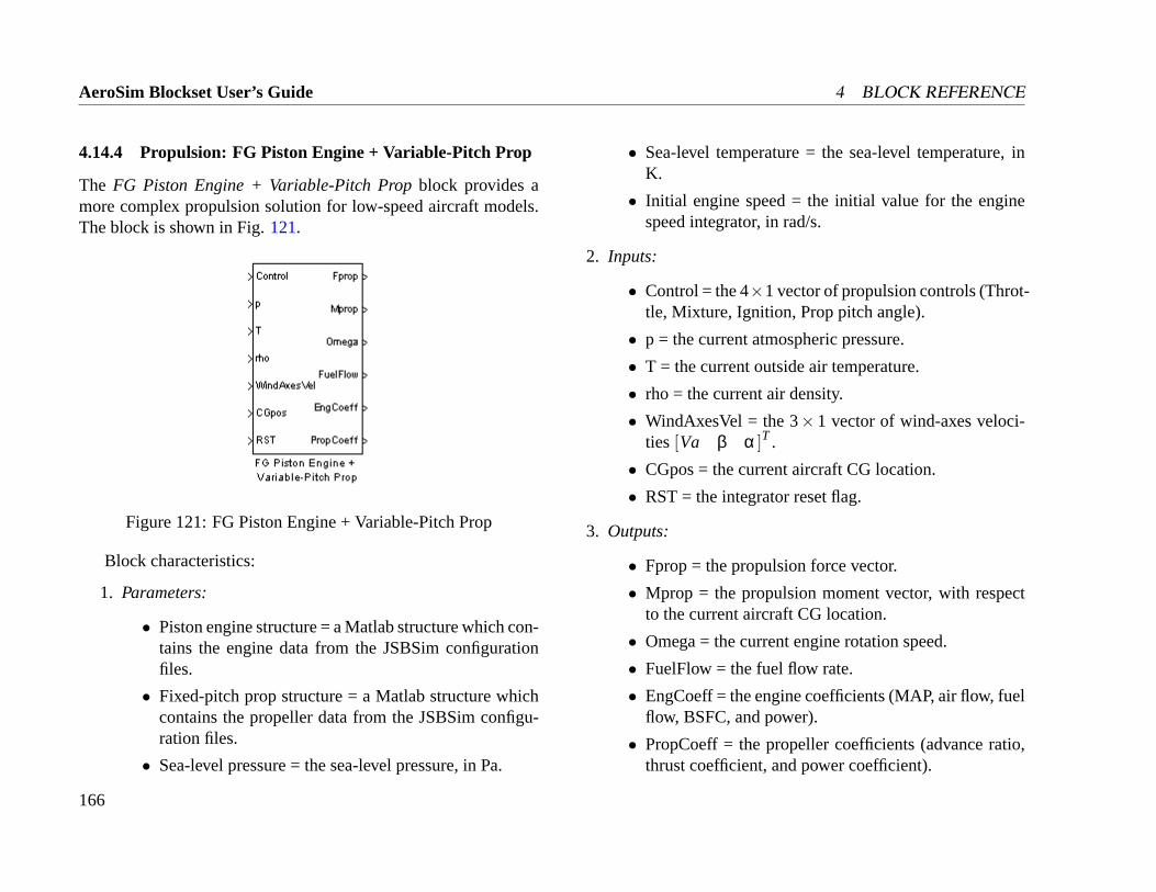
AeroSim Blockset User’s Guide 4 BLOCK REFERENCE
4.14.4 Propulsion: FG Piston Engine + Variable-Pitch Prop
The FG Piston Engine + Variable-Pitch Propblock provides amore complex propulsion solution for low-speed aircraft models.The block is shown in Fig.121.
Figure 121: FG Piston Engine + Variable-Pitch Prop
Block characteristics:
1. Parameters:
• Piston engine structure = a Matlab structure which con-tains the engine data from the JSBSim configurationfiles.
• Fixed-pitch prop structure = a Matlab structure whichcontains the propeller data from the JSBSim configu-ration files.
• Sea-level pressure = the sea-level pressure, in Pa.
• Sea-level temperature = the sea-level temperature, inK.
• Initial engine speed = the initial value for the enginespeed integrator, in rad/s.
2. Inputs:
• Control = the 4×1 vector of propulsion controls (Throt-tle, Mixture, Ignition, Prop pitch angle).
• p = the current atmospheric pressure.
• T = the current outside air temperature.
• rho = the current air density.
• WindAxesVel = the 3×1 vector of wind-axes veloci-ties[Va β α ]T .
• CGpos = the current aircraft CG location.
• RST = the integrator reset flag.
3. Outputs:
• Fprop = the propulsion force vector.
• Mprop = the propulsion moment vector, with respectto the current aircraft CG location.
• Omega = the current engine rotation speed.
• FuelFlow = the fuel flow rate.
• EngCoeff = the engine coefficients (MAP, air flow, fuelflow, BSFC, and power).
• PropCoeff = the propeller coefficients (advance ratio,thrust coefficient, and power coefficient).
166
4 BLOCK REFERENCE AeroSim Blockset User’s Guide
4. Details: The block includes links to theFG Piston Engineand to theFG Variable-Pitch Propellerblocks which can befound in theAeroSim library. The block integrates the an-gular acceleration obtained from the difference between theavailable engine torque and the required propeller torque,by dividing it by the moment of inertia of the rotating com-ponents. Typically the moment of the inertia of the engineshaft is small compared to the propeller moment of inertia,so it can be ignored.
5. Usage:The block is used to model a single propulsion unitand its resulting forces and moments. Multi-engine aircraftwill use multiple blocks of this type.
167
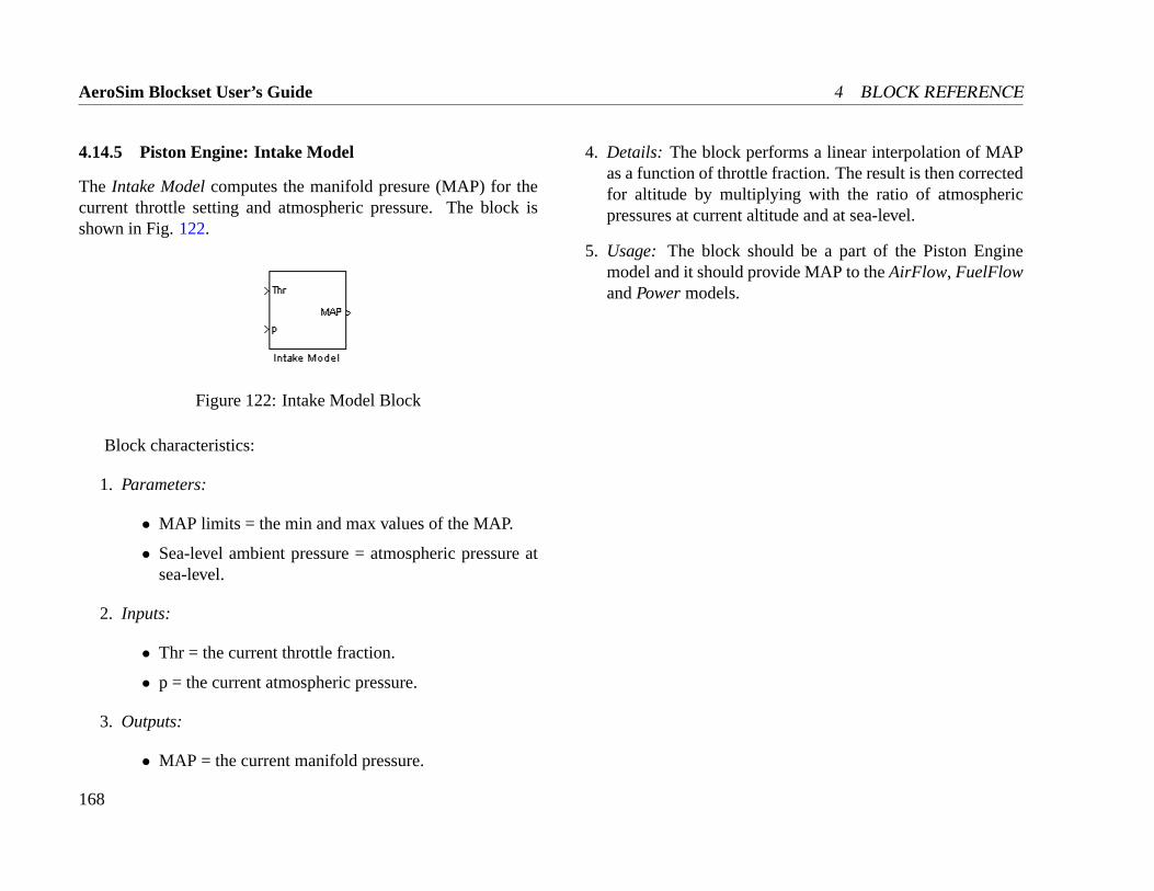
AeroSim Blockset User’s Guide 4 BLOCK REFERENCE
4.14.5 Piston Engine: Intake Model
The Intake Modelcomputes the manifold presure (MAP) for thecurrent throttle setting and atmospheric pressure. The block isshown in Fig.122.
Figure 122: Intake Model Block
Block characteristics:
1. Parameters:
• MAP limits = the min and max values of the MAP.
• Sea-level ambient pressure = atmospheric pressure atsea-level.
2. Inputs:
• Thr = the current throttle fraction.
• p = the current atmospheric pressure.
3. Outputs:
• MAP = the current manifold pressure.
4. Details: The block performs a linear interpolation of MAPas a function of throttle fraction. The result is then correctedfor altitude by multiplying with the ratio of atmosphericpressures at current altitude and at sea-level.
5. Usage: The block should be a part of the Piston Enginemodel and it should provide MAP to theAirFlow, FuelFlowandPowermodels.
168
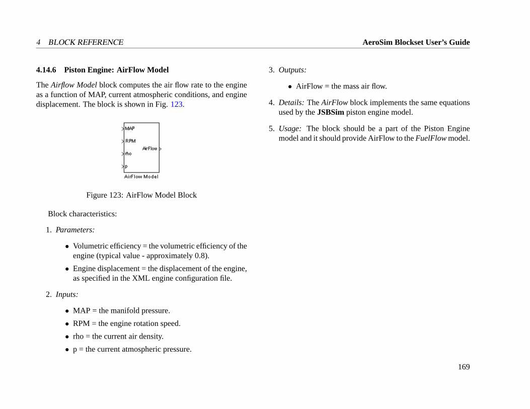
4 BLOCK REFERENCE AeroSim Blockset User’s Guide
4.14.6 Piston Engine: AirFlow Model
TheAirflow Modelblock computes the air flow rate to the engineas a function of MAP, current atmospheric conditions, and enginedisplacement. The block is shown in Fig.123.
Figure 123: AirFlow Model Block
Block characteristics:
1. Parameters:
• Volumetric efficiency = the volumetric efficiency of theengine (typical value - approximately 0.8).
• Engine displacement = the displacement of the engine,as specified in the XML engine configuration file.
2. Inputs:
• MAP = the manifold pressure.
• RPM = the engine rotation speed.
• rho = the current air density.
• p = the current atmospheric pressure.
3. Outputs:
• AirFlow = the mass air flow.
4. Details: TheAirFlow block implements the same equationsused by theJSBSimpiston engine model.
5. Usage: The block should be a part of the Piston Enginemodel and it should provide AirFlow to theFuelFlowmodel.
169
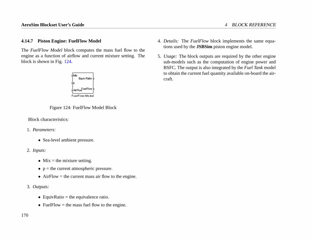
AeroSim Blockset User’s Guide 4 BLOCK REFERENCE
4.14.7 Piston Engine: FuelFlow Model
The FuelFlow Modelblock computes the mass fuel flow to theengine as a function of airflow and current mixture setting. Theblock is shown in Fig.124.
Figure 124: FuelFlow Model Block
Block characteristics:
1. Parameters:
• Sea-level ambient pressure.
2. Inputs:
• Mix = the mixture setting.
• p = the current atmospheric pressure.
• AirFlow = the current mass air flow to the engine.
3. Outputs:
• EquivRatio = the equivalence ratio.
• FuelFlow = the mass fuel flow to the engine.
4. Details: The FuelFlow block implements the same equa-tions used by theJSBSimpiston engine model.
5. Usage:The block outputs are required by the other enginesub-models such as the computation of engine power andBSFC. The output is also integrated by theFuel Tankmodelto obtain the current fuel quantity available on-board the air-craft.
170
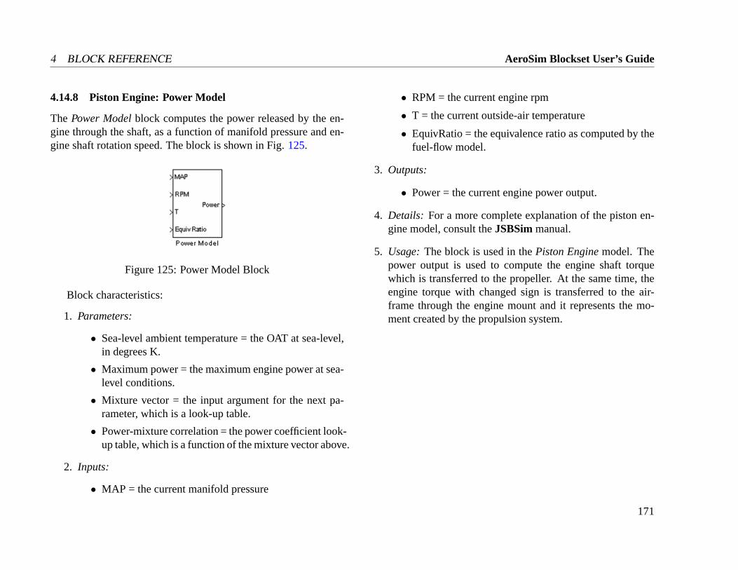
4 BLOCK REFERENCE AeroSim Blockset User’s Guide
4.14.8 Piston Engine: Power Model
The Power Modelblock computes the power released by the en-gine through the shaft, as a function of manifold pressure and en-gine shaft rotation speed. The block is shown in Fig.125.
Figure 125: Power Model Block
Block characteristics:
1. Parameters:
• Sea-level ambient temperature = the OAT at sea-level,in degrees K.
• Maximum power = the maximum engine power at sea-level conditions.
• Mixture vector = the input argument for the next pa-rameter, which is a look-up table.
• Power-mixture correlation = the power coefficient look-up table, which is a function of the mixture vector above.
2. Inputs:
• MAP = the current manifold pressure
• RPM = the current engine rpm
• T = the current outside-air temperature
• EquivRatio = the equivalence ratio as computed by thefuel-flow model.
3. Outputs:
• Power = the current engine power output.
4. Details: For a more complete explanation of the piston en-gine model, consult theJSBSimmanual.
5. Usage:The block is used in thePiston Enginemodel. Thepower output is used to compute the engine shaft torquewhich is transferred to the propeller. At the same time, theengine torque with changed sign is transferred to the air-frame through the engine mount and it represents the mo-ment created by the propulsion system.
171
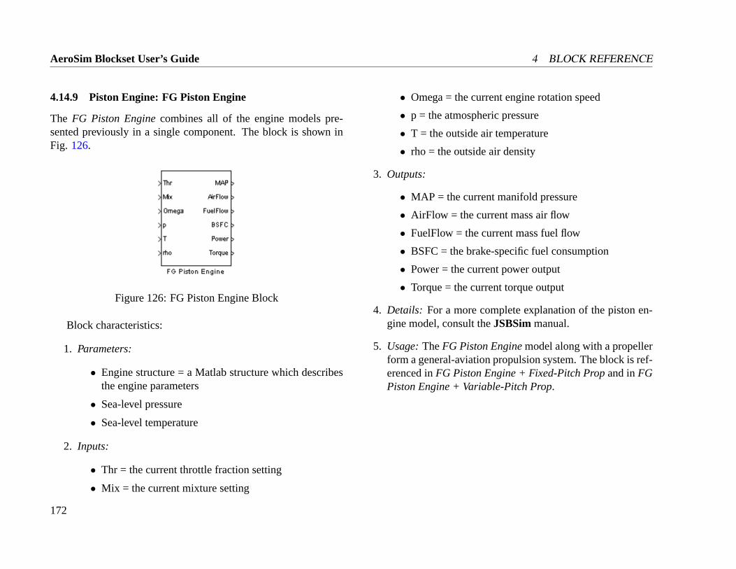
AeroSim Blockset User’s Guide 4 BLOCK REFERENCE
4.14.9 Piston Engine: FG Piston Engine
The FG Piston Enginecombines all of the engine models pre-sented previously in a single component. The block is shown inFig. 126.
Figure 126: FG Piston Engine Block
Block characteristics:
1. Parameters:
• Engine structure = a Matlab structure which describesthe engine parameters
• Sea-level pressure
• Sea-level temperature
2. Inputs:
• Thr = the current throttle fraction setting
• Mix = the current mixture setting
• Omega = the current engine rotation speed
• p = the atmospheric pressure
• T = the outside air temperature
• rho = the outside air density
3. Outputs:
• MAP = the current manifold pressure
• AirFlow = the current mass air flow
• FuelFlow = the current mass fuel flow
• BSFC = the brake-specific fuel consumption
• Power = the current power output
• Torque = the current torque output
4. Details: For a more complete explanation of the piston en-gine model, consult theJSBSimmanual.
5. Usage:TheFG Piston Enginemodel along with a propellerform a general-aviation propulsion system. The block is ref-erenced inFG Piston Engine + Fixed-Pitch Propand inFGPiston Engine + Variable-Pitch Prop.
172
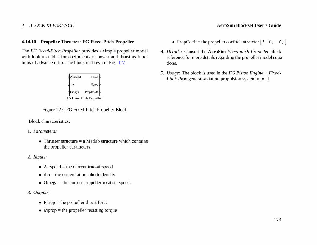
4 BLOCK REFERENCE AeroSim Blockset User’s Guide
4.14.10 Propeller Thruster: FG Fixed-Pitch Propeller
TheFG Fixed-Pitch Propellerprovides a simple propeller modelwith look-up tables for coefficients of power and thrust as func-tions of advance ratio. The block is shown in Fig.127.
Figure 127: FG Fixed-Pitch Propeller Block
Block characteristics:
1. Parameters:
• Thruster structure = a Matlab structure which containsthe propeller parameters.
2. Inputs:
• Airspeed = the current true-airspeed
• rho = the current atmospheric density
• Omega = the current propeller rotation speed.
3. Outputs:
• Fprop = the propeller thrust force
• Mprop = the propeller resisting torque
• PropCoeff = the propeller coefficient vector[J CT CP ]
4. Details: Consult theAeroSim Fixed-pitch Propellerblockreference for more details regarding the propeller model equa-tions.
5. Usage:The block is used in theFG Piston Engine + Fixed-Pitch Propgeneral-aviation propulsion system model.
173
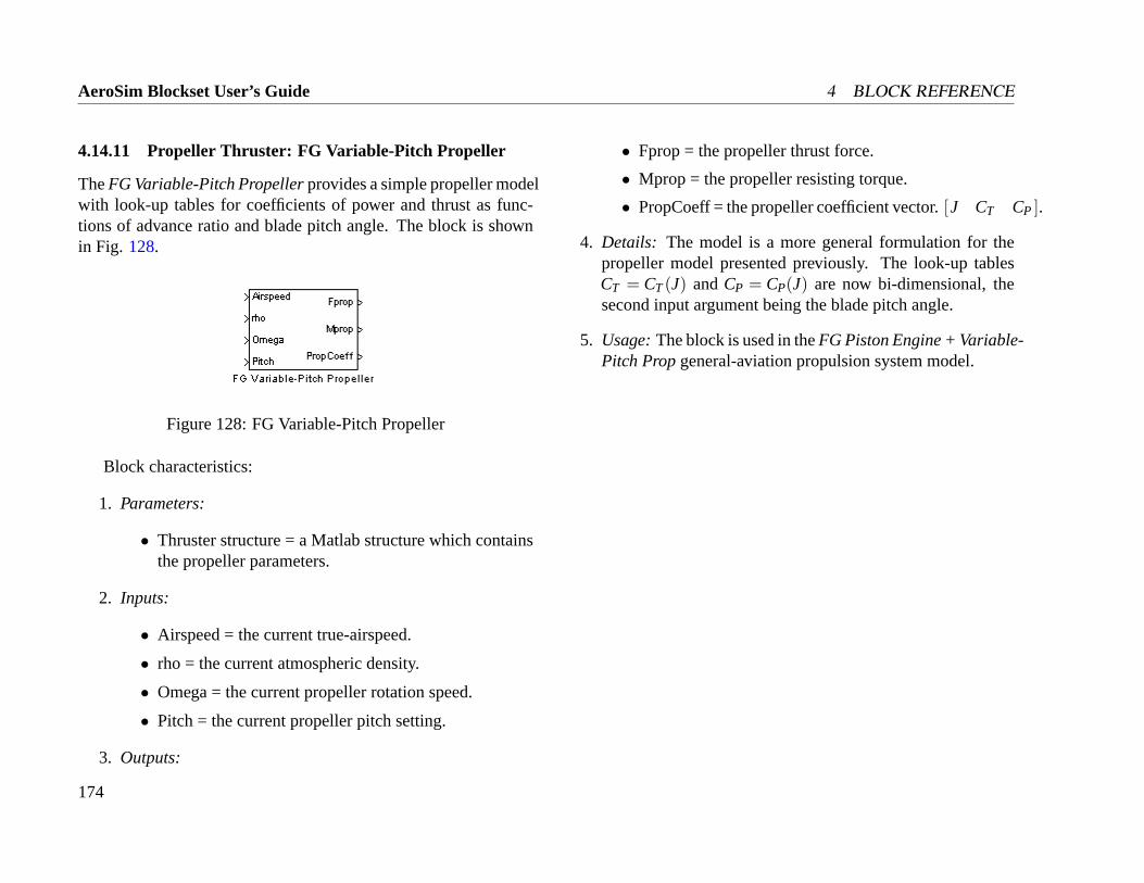
AeroSim Blockset User’s Guide 4 BLOCK REFERENCE
4.14.11 Propeller Thruster: FG Variable-Pitch Propeller
TheFG Variable-Pitch Propellerprovides a simple propeller modelwith look-up tables for coefficients of power and thrust as func-tions of advance ratio and blade pitch angle. The block is shownin Fig. 128.
Figure 128: FG Variable-Pitch Propeller
Block characteristics:
1. Parameters:
• Thruster structure = a Matlab structure which containsthe propeller parameters.
2. Inputs:
• Airspeed = the current true-airspeed.
• rho = the current atmospheric density.
• Omega = the current propeller rotation speed.
• Pitch = the current propeller pitch setting.
3. Outputs:
• Fprop = the propeller thrust force.
• Mprop = the propeller resisting torque.
• PropCoeff = the propeller coefficient vector.[J CT CP ].
4. Details: The model is a more general formulation for thepropeller model presented previously. The look-up tablesCT = CT(J) andCP = CP(J) are now bi-dimensional, thesecond input argument being the blade pitch angle.
5. Usage:The block is used in theFG Piston Engine + Variable-Pitch Propgeneral-aviation propulsion system model.
174
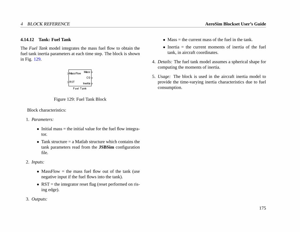
4 BLOCK REFERENCE AeroSim Blockset User’s Guide
4.14.12 Tank: Fuel Tank
The Fuel Tankmodel integrates the mass fuel flow to obtain thefuel tank inertia parameters at each time step. The block is shownin Fig. 129.
Figure 129: Fuel Tank Block
Block characteristics:
1. Parameters:
• Initial mass = the initial value for the fuel flow integra-tor.
• Tank structure = a Matlab structure which contains thetank parameters read from theJSBSim configurationfile.
2. Inputs:
• MassFlow = the mass fuel flow out of the tank (usenegative input if the fuel flows into the tank).
• RST = the integrator reset flag (reset performed on ris-ing edge).
3. Outputs:
• Mass = the current mass of the fuel in the tank.
• Inertia = the current moments of inertia of the fueltank, in aircraft coordinates.
4. Details: The fuel tank model assumes a spherical shape forcomputing the moments of inertia.
5. Usage: The block is used in the aircraft inertia model toprovide the time-varying inertia characteristics due to fuelconsumption.
175
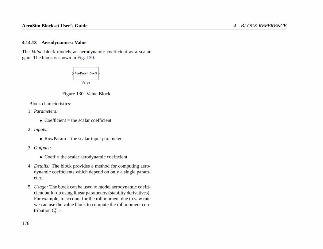
AeroSim Blockset User’s Guide 4 BLOCK REFERENCE
4.14.13 Aerodynamics: Value
The Value block models an aerodynamic coefficient as a scalargain. The block is shown in Fig.130.
Figure 130: Value Block
Block characteristics:
1. Parameters:
• Coefficient = the scalar coefficient
2. Inputs:
• RowParam = the scalar input parameter
3. Outputs:
• Coeff = the scalar aerodynamic coefficient
4. Details: The block provides a method for computing aero-dynamic coefficients which depend on only a single param-eter.
5. Usage:The block can be used to model aerodynamic coeffi-cient build-up using linear parameters (stability derivatives).For example, to account for the roll moment due to yaw ratewe can use the value block to compute the roll moment con-tributionCr
l · r.
176
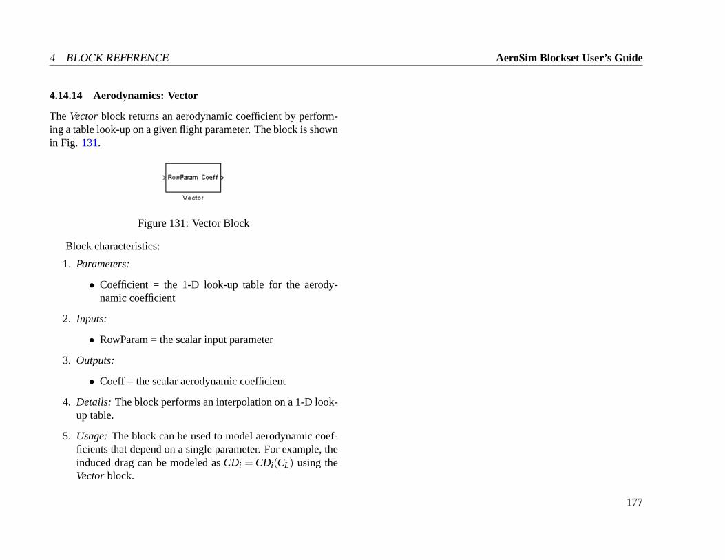
4 BLOCK REFERENCE AeroSim Blockset User’s Guide
4.14.14 Aerodynamics: Vector
TheVectorblock returns an aerodynamic coefficient by perform-ing a table look-up on a given flight parameter. The block is shownin Fig. 131.
Figure 131: Vector Block
Block characteristics:
1. Parameters:
• Coefficient = the 1-D look-up table for the aerody-namic coefficient
2. Inputs:
• RowParam = the scalar input parameter
3. Outputs:
• Coeff = the scalar aerodynamic coefficient
4. Details: The block performs an interpolation on a 1-D look-up table.
5. Usage:The block can be used to model aerodynamic coef-ficients that depend on a single parameter. For example, theinduced drag can be modeled asCDi = CDi(CL) using theVectorblock.
177
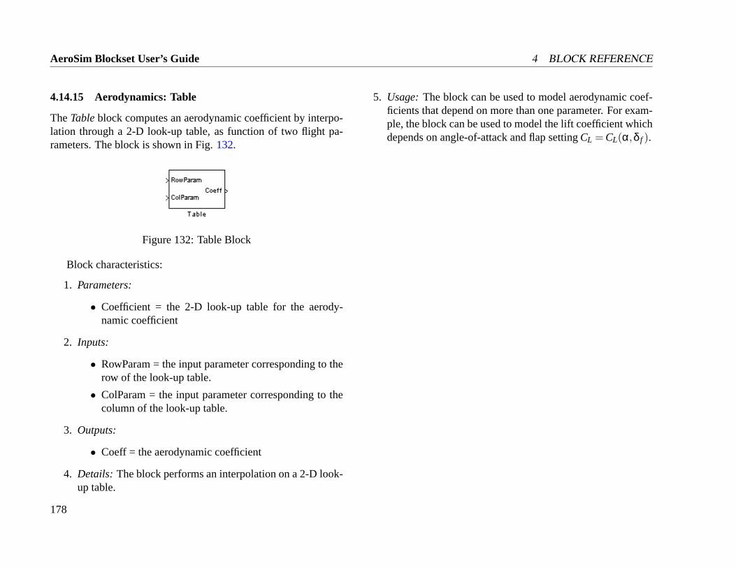
AeroSim Blockset User’s Guide 4 BLOCK REFERENCE
4.14.15 Aerodynamics: Table
TheTableblock computes an aerodynamic coefficient by interpo-lation through a 2-D look-up table, as function of two flight pa-rameters. The block is shown in Fig.132.
Figure 132: Table Block
Block characteristics:
1. Parameters:
• Coefficient = the 2-D look-up table for the aerody-namic coefficient
2. Inputs:
• RowParam = the input parameter corresponding to therow of the look-up table.
• ColParam = the input parameter corresponding to thecolumn of the look-up table.
3. Outputs:
• Coeff = the aerodynamic coefficient
4. Details: The block performs an interpolation on a 2-D look-up table.
5. Usage:The block can be used to model aerodynamic coef-ficients that depend on more than one parameter. For exam-ple, the block can be used to model the lift coefficient whichdepends on angle-of-attack and flap settingCL = CL(α,δ f ).
178
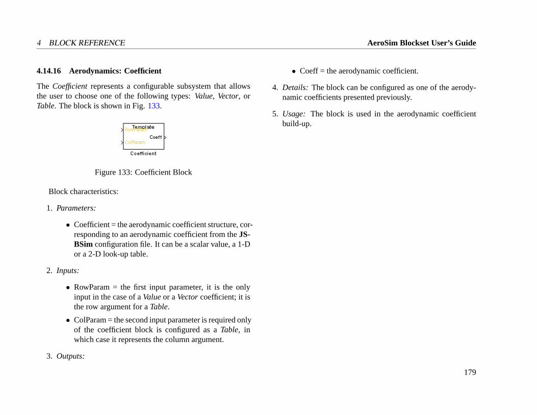
4 BLOCK REFERENCE AeroSim Blockset User’s Guide
4.14.16 Aerodynamics: Coefficient
The Coefficientrepresents a configurable subsystem that allowsthe user to choose one of the following types:Value, Vector, orTable. The block is shown in Fig.133.
Figure 133: Coefficient Block
Block characteristics:
1. Parameters:
• Coefficient = the aerodynamic coefficient structure, cor-responding to an aerodynamic coefficient from theJS-BSim configuration file. It can be a scalar value, a 1-Dor a 2-D look-up table.
2. Inputs:
• RowParam = the first input parameter, it is the onlyinput in the case of aValueor aVectorcoefficient; it isthe row argument for aTable.
• ColParam = the second input parameter is required onlyof the coefficient block is configured as aTable, inwhich case it represents the column argument.
3. Outputs:
• Coeff = the aerodynamic coefficient.
4. Details: The block can be configured as one of the aerody-namic coefficients presented previously.
5. Usage: The block is used in the aerodynamic coefficientbuild-up.
179
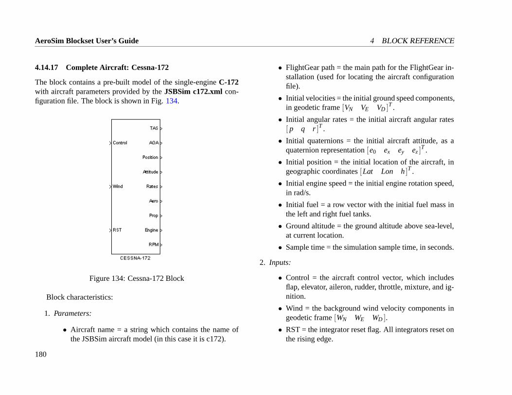
AeroSim Blockset User’s Guide 4 BLOCK REFERENCE
4.14.17 Complete Aircraft: Cessna-172
The block contains a pre-built model of the single-engineC-172with aircraft parameters provided by theJSBSim c172.xmlcon-figuration file. The block is shown in Fig.134.
Figure 134: Cessna-172 Block
Block characteristics:
1. Parameters:
• Aircraft name = a string which contains the name ofthe JSBSim aircraft model (in this case it is c172).
• FlightGear path = the main path for the FlightGear in-stallation (used for locating the aircraft configurationfile).
• Initial velocities = the initial ground speed components,in geodetic frame[VN VE VD ]T .
• Initial angular rates = the initial aircraft angular rates[ p q r]T .
• Initial quaternions = the initial aircraft attitude, as aquaternion representation[e0 ex ey ez]
T .
• Initial position = the initial location of the aircraft, ingeographic coordinates[Lat Lon h]T .
• Initial engine speed = the initial engine rotation speed,in rad/s.
• Initial fuel = a row vector with the initial fuel mass inthe left and right fuel tanks.
• Ground altitude = the ground altitude above sea-level,at current location.
• Sample time = the simulation sample time, in seconds.
2. Inputs:
• Control = the aircraft control vector, which includesflap, elevator, aileron, rudder, throttle, mixture, and ig-nition.
• Wind = the background wind velocity components ingeodetic frame[WN WE WD ].
• RST = the integrator reset flag. All integrators reset onthe rising edge.
180
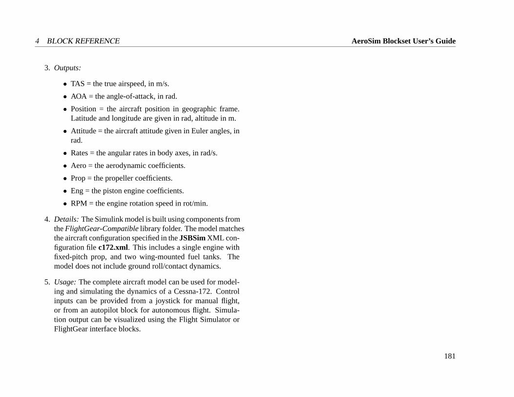
4 BLOCK REFERENCE AeroSim Blockset User’s Guide
3. Outputs:
• TAS = the true airspeed, in m/s.
• AOA = the angle-of-attack, in rad.
• Position = the aircraft position in geographic frame.Latitude and longitude are given in rad, altitude in m.
• Attitude = the aircraft attitude given in Euler angles, inrad.
• Rates = the angular rates in body axes, in rad/s.
• Aero = the aerodynamic coefficients.
• Prop = the propeller coefficients.
• Eng = the piston engine coefficients.
• RPM = the engine rotation speed in rot/min.
4. Details: The Simulink model is built using components fromtheFlightGear-Compatiblelibrary folder. The model matchesthe aircraft configuration specified in theJSBSimXML con-figuration filec172.xml. This includes a single engine withfixed-pitch prop, and two wing-mounted fuel tanks. Themodel does not include ground roll/contact dynamics.
5. Usage:The complete aircraft model can be used for model-ing and simulating the dynamics of a Cessna-172. Controlinputs can be provided from a joystick for manual flight,or from an autopilot block for autonomous flight. Simula-tion output can be visualized using the Flight Simulator orFlightGear interface blocks.
181
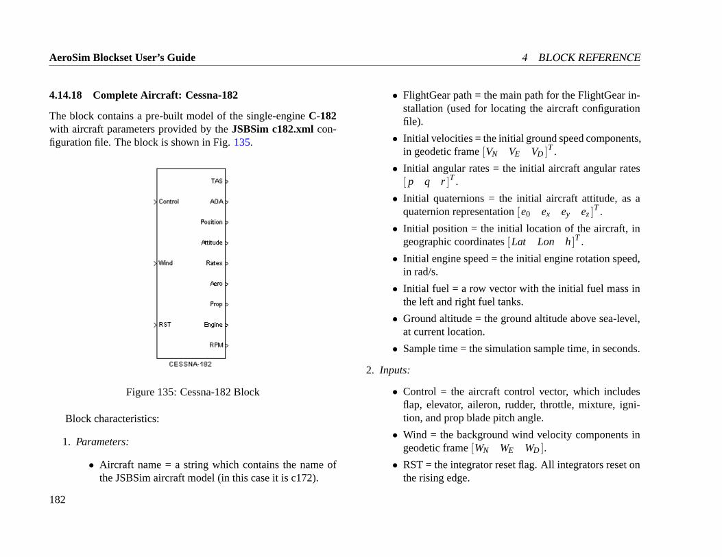
AeroSim Blockset User’s Guide 4 BLOCK REFERENCE
4.14.18 Complete Aircraft: Cessna-182
The block contains a pre-built model of the single-engineC-182with aircraft parameters provided by theJSBSim c182.xmlcon-figuration file. The block is shown in Fig.135.
Figure 135: Cessna-182 Block
Block characteristics:
1. Parameters:
• Aircraft name = a string which contains the name ofthe JSBSim aircraft model (in this case it is c172).
• FlightGear path = the main path for the FlightGear in-stallation (used for locating the aircraft configurationfile).
• Initial velocities = the initial ground speed components,in geodetic frame[VN VE VD ]T .
• Initial angular rates = the initial aircraft angular rates[ p q r]T .
• Initial quaternions = the initial aircraft attitude, as aquaternion representation[e0 ex ey ez]
T .
• Initial position = the initial location of the aircraft, ingeographic coordinates[Lat Lon h]T .
• Initial engine speed = the initial engine rotation speed,in rad/s.
• Initial fuel = a row vector with the initial fuel mass inthe left and right fuel tanks.
• Ground altitude = the ground altitude above sea-level,at current location.
• Sample time = the simulation sample time, in seconds.
2. Inputs:
• Control = the aircraft control vector, which includesflap, elevator, aileron, rudder, throttle, mixture, igni-tion, and prop blade pitch angle.
• Wind = the background wind velocity components ingeodetic frame[WN WE WD ].
• RST = the integrator reset flag. All integrators reset onthe rising edge.
182

4 BLOCK REFERENCE AeroSim Blockset User’s Guide
3. Outputs:
• TAS = the true airspeed, in m/s.
• AOA = the angle-of-attack, in rad.
• Position = the aircraft position in geographic frame.Latitude and longitude are given in rad, altitude in m.
• Attitude = the aircraft attitude given in Euler angles, inrad.
• Rates = the angular rates in body axes, in rad/s.
• Aero = the aerodynamic coefficients.
• Prop = the propeller coefficients.
• Eng = the piston engine coefficients.
• RPM = the engine rotation speed in rot/min.
4. Details: The Simulink model is built using components fromtheFlightGear-Compatiblelibrary folder. The model matchesthe aircraft configuration specified in theJSBSimXML con-figuration filec182.xml. This includes a single engine withvariable-pitch prop, and two wing-mounted fuel tanks. Themodel does not include ground roll/contact dynamics.
5. Usage:The complete aircraft model can be used for model-ing and simulating the dynamics of a Cessna-182. Controlinputs can be provided from a joystick for manual flight,or from an autopilot block for autonomous flight. Simula-tion output can be visualized using the Flight Simulator orFlightGear interface blocks.
183
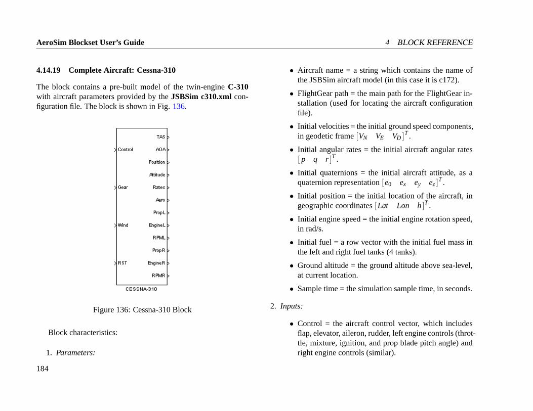
AeroSim Blockset User’s Guide 4 BLOCK REFERENCE
4.14.19 Complete Aircraft: Cessna-310
The block contains a pre-built model of the twin-engineC-310with aircraft parameters provided by theJSBSim c310.xmlcon-figuration file. The block is shown in Fig.136.
Figure 136: Cessna-310 Block
Block characteristics:
1. Parameters:
• Aircraft name = a string which contains the name ofthe JSBSim aircraft model (in this case it is c172).
• FlightGear path = the main path for the FlightGear in-stallation (used for locating the aircraft configurationfile).
• Initial velocities = the initial ground speed components,in geodetic frame[VN VE VD ]T .
• Initial angular rates = the initial aircraft angular rates[ p q r]T .
• Initial quaternions = the initial aircraft attitude, as aquaternion representation[e0 ex ey ez]
T .
• Initial position = the initial location of the aircraft, ingeographic coordinates[Lat Lon h]T .
• Initial engine speed = the initial engine rotation speed,in rad/s.
• Initial fuel = a row vector with the initial fuel mass inthe left and right fuel tanks (4 tanks).
• Ground altitude = the ground altitude above sea-level,at current location.
• Sample time = the simulation sample time, in seconds.
2. Inputs:
• Control = the aircraft control vector, which includesflap, elevator, aileron, rudder, left engine controls (throt-tle, mixture, ignition, and prop blade pitch angle) andright engine controls (similar).
184
4 BLOCK REFERENCE AeroSim Blockset User’s Guide
• Gear = the retractable landing gear position, used forcomputing aerodynamic coefficients (1 = gear down, 0= gear up).
• Wind = the background wind velocity components ingeodetic frame[WN WE WD ].
• RST = the integrator reset flag. All integrators reset onthe rising edge.
3. Outputs:
• TAS = the true airspeed, in m/s.
• AOA = the angle-of-attack, in rad.
• Position = the aircraft position in geographic frame.Latitude and longitude are given in rad, altitude in m.
• Attitude = the aircraft attitude given in Euler angles, inrad.
• Rates = the angular rates in body axes, in rad/s.
• Aero = the aerodynamic coefficients.
• PropL = the left propeller coefficients.
• EngL = the left piston engine coefficients.
• RPML = the left engine rotation speed in rot/min.
• PropR = the right propeller coefficients.
• EngR = the right piston engine coefficients.
• RPMR = the right engine rotation speed in rot/min.
4. Details: The Simulink model is built using components fromtheFlightGear-Compatiblelibrary folder. The model matches
the aircraft configuration specified in theJSBSimXML con-figuration file c310.xml. This includes two engines withvariable-pitch props, and four wing-mounted fuel tanks. Themodel does not include ground roll/contact dynamics.
5. Usage:The complete aircraft model can be used for model-ing and simulating the dynamics of a Cessna-310. Controlinputs can be provided from a joystick for manual flight,or from an autopilot block for autonomous flight. Simula-tion output can be visualized using the Flight Simulator orFlightGear interface blocks.
185
AeroSim Blockset User’s Guide REFERENCES
References
[1] Farrell J. A. and Barth M.The Global Positioning System &Inertial Navigation. McGraw Hill, 1999. ISBN 0-07-022045-X.
[2] Phillips W. F. Hailey C. E. and Gebert G. A. Review of At-titude Representations Used for Aircraft Kinematics.Journalof Aircraft, 38:718–737, 2001.
[3] Stevens B. L. and Lewis F. L.Aircraft Control and Simulation.John Wiley & Sons, Inc., 1992. ISBN 0-471-61397-5.
[4] Rogers R. M.Applied Mathematics in Integrated NavigationSystems. American Institute of Aeronautics and Astronautics,Inc., 2000. ISBN 1-56347-397-6.
[5] Smetana F. O.Evaluation of Stability Derivatives.
186