Age-Structured Leslie Matrix Population Modeling Learning Objectives: 1. Set up a model of population growth with age structure. 2. Estimate the geometric growth rate (λ) from Leslie matrix calculations. 3. Determine the stable age distribution (SAD) of the population. 4. Construct and interpret the age distribution graphs. 5. Learn more about how to use the remarkable functionality of Excel

2013 to plot and analyze wildlife population data. Introduction Suppose we want to quantify the growth of the elk population in Arkansas over time. Elk breed annually and we plan to count elk from a helicopter in late winter, prior to green-up, when the animals are most detectible from the air. The growth rate of a population, such as an elk population, over discrete time steps is called the geometric growth rate (λ) and describes abundance next year as a multiple (or proportion) of the abundance this year. The geometric growth rate is convenient to use because it easily converts to % change/year [(λ-1) x 100]. For example, when λ = 1, the population will remain constant in size over time, meaning that it neither increases nor decreases; that is, (1-1) x 100 = 0%. When λ < 1, the population declines geometrically (i.e., If λ = 0.75 the population will be three-quarters the size that it was last year; that is, (0.75-1) x 100 = -25%. When λ > 1, the population increases geometrically (i.e., If λ = 1.25 the population will be one-quarter larger in size than it was last year; that is, (1.25-1) x 100 = 25%. Mathematically, the abundance of a population (N) at time t+1 is a function of both abundance at time t and the population growth rate:

Nt+1 = Nt λ ,

where N is the number of individuals present in the population, and t is a time interval of interest. This equation says that the size of a population at time t+1 is equal to the size of the population at time t multiplied by a constant, λ. Although geometric growth models have been used to describe population growth, like all models they come with a set of assumptions. What are the

Equation 1

2

assumptions of the geometric growth model? The equation describes a population in which there is no genetic structure, no age structure, and no sex structure to the population (Gotelli 2001), and all individuals are reproductively active when the animals are counted. The model also assumes that resources are virtually unlimited and that growth is unaffected by the size of the population (i.e., no density dependence). Can you think of an organism whose life history meets these assumptions? Many natural populations violate at least 1 of these assumptions because wildlife populations have structure: they are composed of individuals whose birth and death rates differ depending on age, sex, or genetic makeup. All else being equal, a population of 1000 individuals that is composed of 350 pre-reproductive-age individuals, 500 reproductive-age individuals, and 150 post-reproductive-age individuals will have a different growth rate than a population where all 1000 individuals are of reproductive age. In this exercise, you will develop a Leslie matrix model to explore the growth of populations that have age structure. This approach will enable you to estimate λ for age-structured populations. Chapter 6 in Mills (2013) contains a very readable and practical discussion of building and analyzing age-structured Leslie matrix population models. Model Notation Let’s begin this exercise looking at some notation often used when modeling populations that are age-structured. For modeling purposes, we divide individuals into groups by either their age or their age class. Although age is a continuous variable when individuals are born throughout the year, by convention (and necessity) individuals are grouped or categorized into discrete time intervals. That is, the age class of 3-year olds consists of individuals that just had their third birthday, plus individuals that are 3.5 years old, 3.8 years old, and so on. In age-structured models, all individuals within a particular age group (e.g., 3-year-olds) are assumed to have the same birth and death rates. By convention, the age of individuals is given by the letter x, followed by a number within parentheses. Thus, newborns are x(0) and 3-year-olds are x(3). In contrast, the age class of an individual is given by the letter i, followed by a subscript number. A newborn enters the first age class upon birth (i1), and enters the second age class upon its first birthday (i2). Caswell (2001) illustrates the relationship between age and age class as:

3

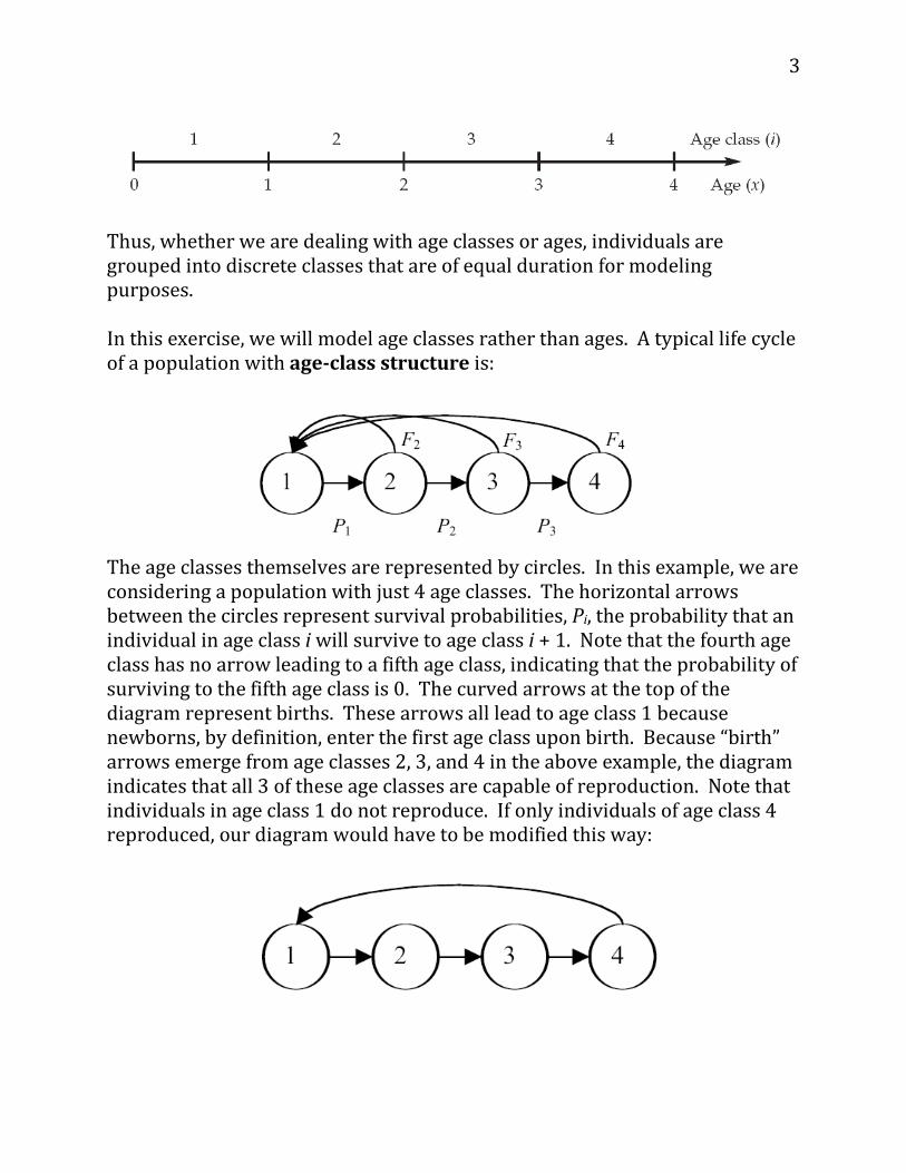
Thus, whether we are dealing with age classes or ages, individuals are grouped into discrete classes that are of equal duration for modeling purposes. In this exercise, we will model age classes rather than ages. A typical life cycle of a population with age-class structure is:

The age classes themselves are represented by circles. In this example, we are considering a population with just 4 age classes. The horizontal arrows between the circles represent survival probabilities, Pi, the probability that an individual in age class i will survive to age class i + 1. Note that the fourth age class has no arrow leading to a fifth age class, indicating that the probability of surviving to the fifth age class is 0. The curved arrows at the top of the diagram represent births. These arrows all lead to age class 1 because newborns, by definition, enter the first age class upon birth. Because “birth” arrows emerge from age classes 2, 3, and 4 in the above example, the diagram indicates that all 3 of these age classes are capable of reproduction. Note that individuals in age class 1 do not reproduce. If only individuals of age class 4 reproduced, our diagram would have to be modified this way:

4

The Leslie Matrix The major goal of a Leslie matrix population modeling is to compute λ. In our matrix model, we can compute the time-specific geometric growth rate as λt. The value of λt can be computed as

𝜆𝜆𝑡𝑡 =𝑁𝑁𝑡𝑡+1𝑁𝑁𝑡𝑡

.

λt is not necessarily the same as λ in Equation 1. We will discuss that issue later. By the way, as you study the material in this section, be sure to keep in mind the biological relevance of what is going on. It is easy to get lost in the details. To determine Nt and Nt+1, we need to count individuals at some standardized time period over time. We will make 2 assumptions in our computations. First, we will assume that the time step between Nt and Nt+1 is 1 year, and that age classes are defined by yearly intervals. If we were interested in a different time step—say, 6 months—then our age classes would also have to be 6-month intervals. Second, we will assume for this exercise that our elk counts are conducted and completed once per year after the elk breeding season (a post-breeding survey). The number of individuals in the population in a survey at time t+1 will depend on how many individuals of each age class were in the population at time t, as well as the birth and survival probabilities for each age class. Let’s start by examining the survival probability, designated by the letter P. P is the probability that an individual in age class i will survive to age class i+1. The small letter l gives the number of individuals in the population in age class i at a given time:

𝑃𝑃𝑖𝑖 =𝑙𝑙(𝑖𝑖)

𝑙𝑙(𝑖𝑖 − 1).

For example, let’s assume the probability that individuals in age class 1 survive to age class 2 is P1 = 0.3. This means 30% of the individuals in age class 1 will survive to be counted as age class 2 individuals. By definition, the remaining 70% of the individuals will die. If we consider survival alone, we

5

can compute the number of individuals of age class 2 at time t+1 as the number of individuals of age class 1 at time t multiplied by P1. If we denote the number of individuals in class i at time t as ni(t), we can write the more general equation as

ni+1(t+1) = Pini(t).

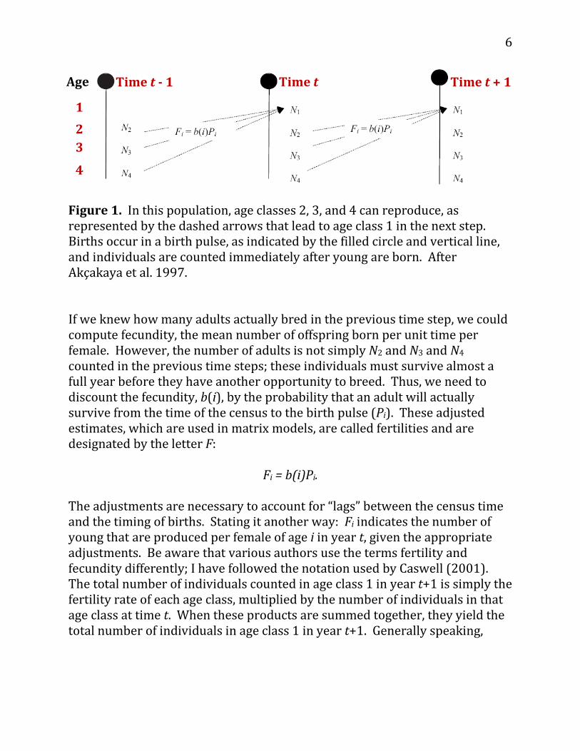
This equation works for calculating the number of individuals at time t+1 for each age class in the population except for the first, because individuals in the first age class arise only through birth. Accordingly, let’s now consider birth rates. There are many ways to describe the occurrence of births in a population. Here, we will assume a simple birth-pulse model in which individuals give birth the moment they enter a new age class. When populations are structured, the birth rate is called the fecundity, or the mean number of offspring born per unit time to an individual female of a particular age. In the exercise on life tables, recall that fecundity was labeled as b(x), where b was for birth. Individuals that are of pre-reproductive or post-reproductive age have fecundities of 0. Individuals of reproductive age typically have fecundities >0. Figure 1 is a hypothetical diagram of a population with 4 age classes (1-4) that are surveyed at 3 time periods: time t–1, time t, and time t+1. All individuals “graduate” to the next age class on their birthday, and since all individuals have roughly the same birthday, all individuals counted in the survey are “fresh”; that is, the newborns were just born, individuals in age class 2 just entered age class 2, and so forth. Note that the number of individuals in the first age class at time t depends on the number of breeding adults in the previous time step.

6

Figure 1. In this population, age classes 2, 3, and 4 can reproduce, as represented by the dashed arrows that lead to age class 1 in the next step. Births occur in a birth pulse, as indicated by the filled circle and vertical line, and individuals are counted immediately after young are born. After Akçakaya et al. 1997. If we knew how many adults actually bred in the previous time step, we could compute fecundity, the mean number of offspring born per unit time per female. However, the number of adults is not simply N2 and N3 and N4 counted in the previous time steps; these individuals must survive almost a full year before they have another opportunity to breed. Thus, we need to discount the fecundity, b(i), by the probability that an adult will actually survive from the time of the census to the birth pulse (Pi). These adjusted estimates, which are used in matrix models, are called fertilities and are designated by the letter F:

Fi = b(i)Pi. The adjustments are necessary to account for “lags” between the census time and the timing of births. Stating it another way: Fi indicates the number of young that are produced per female of age i in year t, given the appropriate adjustments. Be aware that various authors use the terms fertility and fecundity differently; I have followed the notation used by Caswell (2001). The total number of individuals counted in age class 1 in year t+1 is simply the fertility rate of each age class, multiplied by the number of individuals in that age class at time t. When these products are summed together, they yield the total number of individuals in age class 1 in year t+1. Generally speaking,

Time t - 1 Time t Time t + 1 1

2 3

4

Age

7

𝑛𝑛1(𝑡𝑡 + 1) = �𝐹𝐹𝑖𝑖𝑛𝑛𝑖𝑖(𝑡𝑡)𝑘𝑘

𝑖𝑖=1

.

Once we know the fertility and survivorship coefficients for each age class, we can calculate the number of individuals in each age at time t+1, given the number of individuals in each class at time t:

n1(t+1) = F1n1(t) + F2n2(t) + F3n3(t) + F4n4(t) n2(t+1) = P1n1(t) n3(t+1) = P2n2(t) n4(t+1) = P3n3(t)

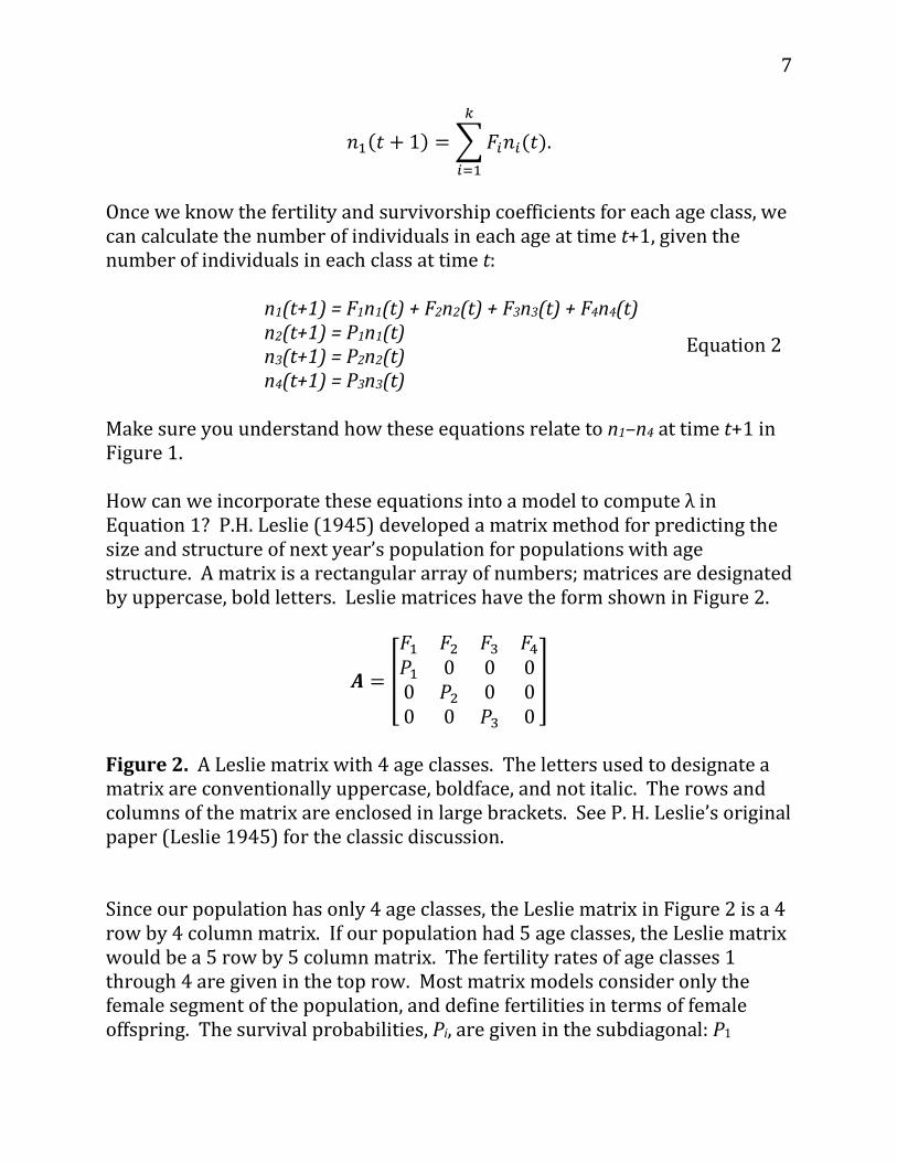
Make sure you understand how these equations relate to n1–n4 at time t+1 in Figure 1. How can we incorporate these equations into a model to compute λ in Equation 1? P.H. Leslie (1945) developed a matrix method for predicting the size and structure of next year’s population for populations with age structure. A matrix is a rectangular array of numbers; matrices are designated by uppercase, bold letters. Leslie matrices have the form shown in Figure 2.

𝑨𝑨 = �

𝐹𝐹1 𝐹𝐹2 𝐹𝐹3 𝐹𝐹4𝑃𝑃1 0 0 00 𝑃𝑃2 0 00 0 𝑃𝑃3 0

�

Figure 2. A Leslie matrix with 4 age classes. The letters used to designate a matrix are conventionally uppercase, boldface, and not italic. The rows and columns of the matrix are enclosed in large brackets. See P. H. Leslie’s original paper (Leslie 1945) for the classic discussion. Since our population has only 4 age classes, the Leslie matrix in Figure 2 is a 4 row by 4 column matrix. If our population had 5 age classes, the Leslie matrix would be a 5 row by 5 column matrix. The fertility rates of age classes 1 through 4 are given in the top row. Most matrix models consider only the female segment of the population, and define fertilities in terms of female offspring. The survival probabilities, Pi, are given in the subdiagonal: P1

Equation 2

8

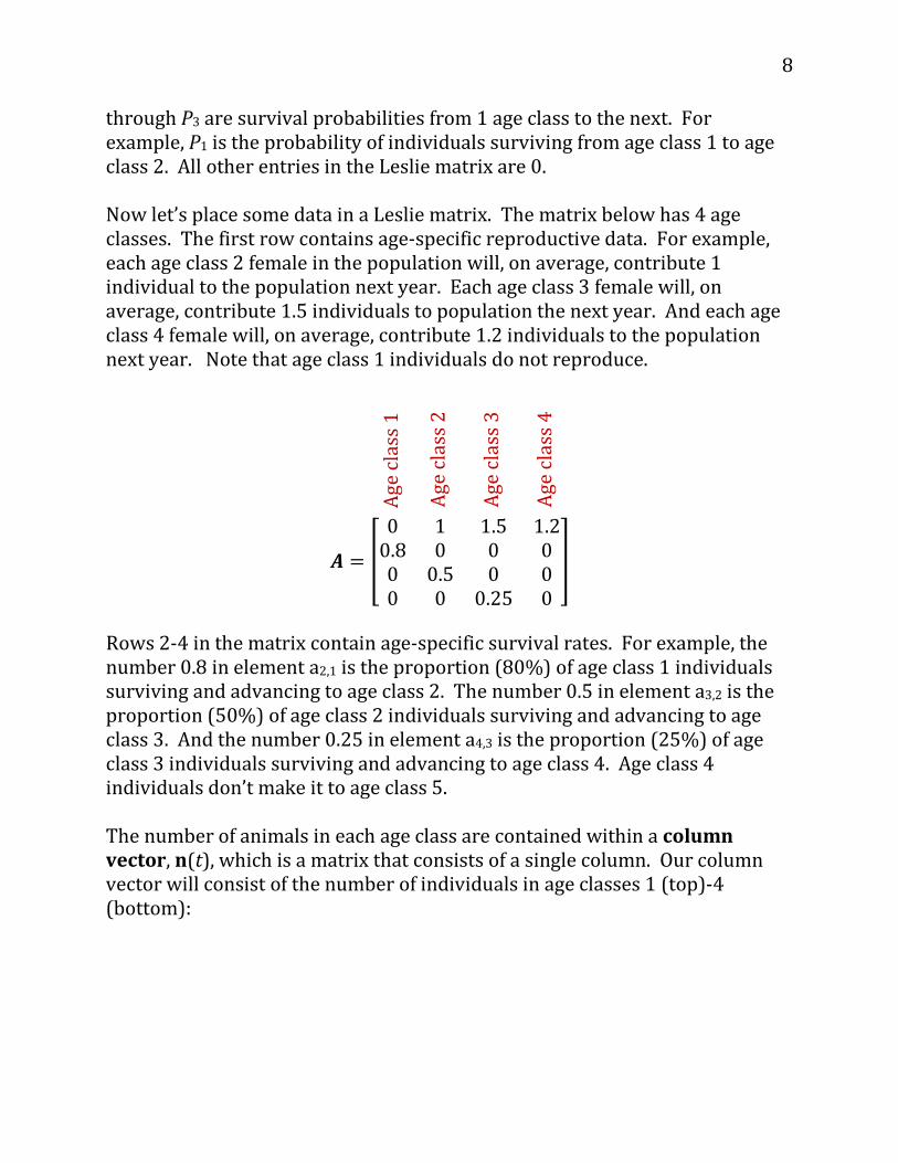
through P3 are survival probabilities from 1 age class to the next. For example, P1 is the probability of individuals surviving from age class 1 to age class 2. All other entries in the Leslie matrix are 0. Now let’s place some data in a Leslie matrix. The matrix below has 4 age classes. The first row contains age-specific reproductive data. For example, each age class 2 female in the population will, on average, contribute 1 individual to the population next year. Each age class 3 female will, on average, contribute 1.5 individuals to population the next year. And each age class 4 female will, on average, contribute 1.2 individuals to the population next year. Note that age class 1 individuals do not reproduce.

𝑨𝑨 = �

0 1 1.5 1.20.8 0 0 00 0.5 0 00 0 0.25 0

�

Rows 2-4 in the matrix contain age-specific survival rates. For example, the number 0.8 in element a2,1 is the proportion (80%) of age class 1 individuals surviving and advancing to age class 2. The number 0.5 in element a3,2 is the proportion (50%) of age class 2 individuals surviving and advancing to age class 3. And the number 0.25 in element a4,3 is the proportion (25%) of age class 3 individuals surviving and advancing to age class 4. Age class 4 individuals don’t make it to age class 5. The number of animals in each age class are contained within a column vector, n(t), which is a matrix that consists of a single column. Our column vector will consist of the number of individuals in age classes 1 (top)-4 (bottom):

Age

clas

s 1

Age

clas

s 2

Age

clas

s 3

Age

clas

s 4

9

𝐧𝐧(𝑡𝑡) = �

𝑤𝑤𝑥𝑥𝑦𝑦𝑧𝑧

�

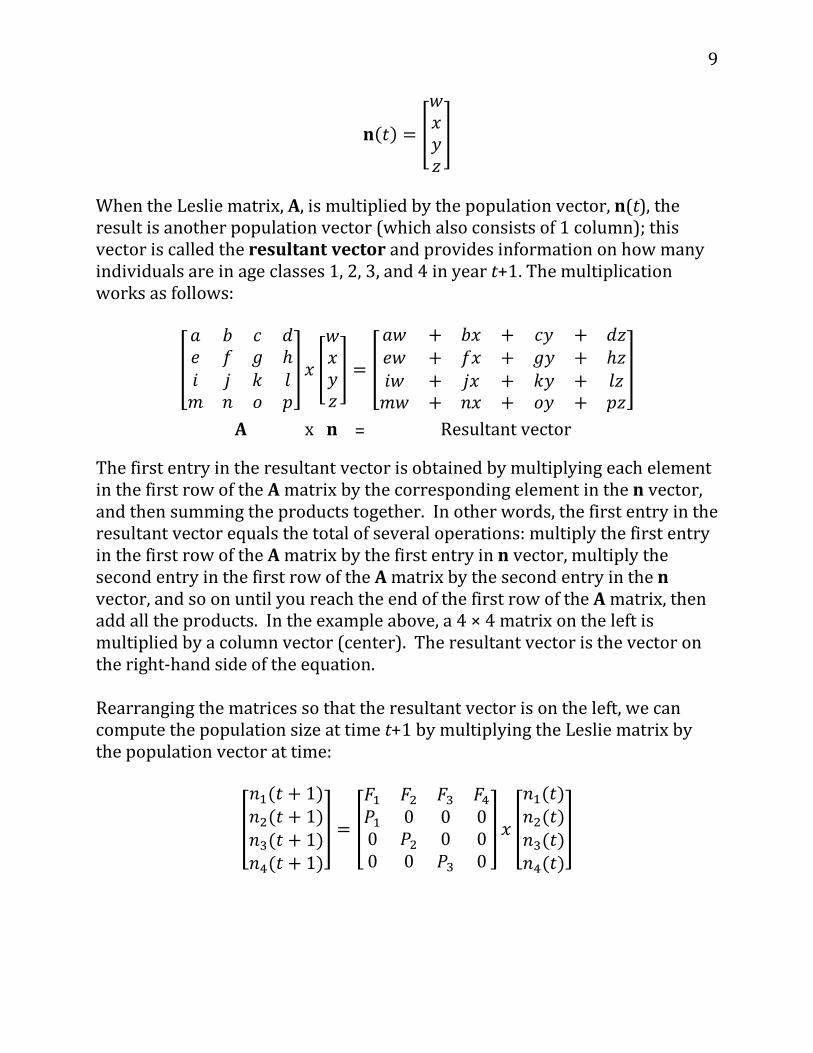
When the Leslie matrix, A, is multiplied by the population vector, n(t), the result is another population vector (which also consists of 1 column); this vector is called the resultant vector and provides information on how many individuals are in age classes 1, 2, 3, and 4 in year t+1. The multiplication works as follows:

�

𝑎𝑎 𝑏𝑏 𝑐𝑐 𝑑𝑑𝑒𝑒 𝑓𝑓 𝑔𝑔 ℎ𝑖𝑖 𝑗𝑗 𝑘𝑘 𝑙𝑙𝑚𝑚 𝑛𝑛 𝑜𝑜 𝑝𝑝

�𝑥𝑥 �

𝑤𝑤𝑥𝑥𝑦𝑦𝑧𝑧

� = �

𝑎𝑎𝑤𝑤 + 𝑏𝑏𝑥𝑥 + 𝑐𝑐𝑦𝑦 + 𝑑𝑑𝑧𝑧𝑒𝑒𝑤𝑤 + 𝑓𝑓𝑥𝑥 + 𝑔𝑔𝑦𝑦 + ℎ𝑧𝑧𝑖𝑖𝑤𝑤 + 𝑗𝑗𝑥𝑥 + 𝑘𝑘𝑦𝑦 + 𝑙𝑙𝑧𝑧𝑚𝑚𝑤𝑤 + 𝑛𝑛𝑥𝑥 + 𝑜𝑜𝑦𝑦 + 𝑝𝑝𝑧𝑧

�

The first entry in the resultant vector is obtained by multiplying each element in the first row of the A matrix by the corresponding element in the n vector, and then summing the products together. In other words, the first entry in the resultant vector equals the total of several operations: multiply the first entry in the first row of the A matrix by the first entry in n vector, multiply the second entry in the first row of the A matrix by the second entry in the n vector, and so on until you reach the end of the first row of the A matrix, then add all the products. In the example above, a 4 × 4 matrix on the left is multiplied by a column vector (center). The resultant vector is the vector on the right-hand side of the equation. Rearranging the matrices so that the resultant vector is on the left, we can compute the population size at time t+1 by multiplying the Leslie matrix by the population vector at time:

�

𝑛𝑛1(𝑡𝑡 + 1)𝑛𝑛2(𝑡𝑡 + 1)𝑛𝑛3(𝑡𝑡 + 1)𝑛𝑛4(𝑡𝑡 + 1)

� = �

𝐹𝐹1 𝐹𝐹2 𝐹𝐹3 𝐹𝐹4𝑃𝑃1 0 0 00 𝑃𝑃2 0 00 0 𝑃𝑃3 0

� 𝑥𝑥 �

𝑛𝑛1(𝑡𝑡)𝑛𝑛2(𝑡𝑡)𝑛𝑛3(𝑡𝑡)𝑛𝑛4(𝑡𝑡)

�

A x = n Resultant vector

10

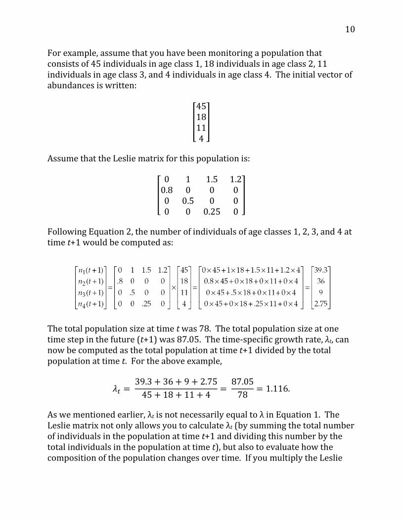
For example, assume that you have been monitoring a population that consists of 45 individuals in age class 1, 18 individuals in age class 2, 11 individuals in age class 3, and 4 individuals in age class 4. The initial vector of abundances is written:

�

4518114

�

Assume that the Leslie matrix for this population is:

�

0 1 1.5 1.20.8 0 0 00 0.5 0 00 0 0.25 0

�

Following Equation 2, the number of individuals of age classes 1, 2, 3, and 4 at time t+1 would be computed as:

The total population size at time t was 78. The total population size at one time step in the future (t+1) was 87.05. The time-specific growth rate, λt, can now be computed as the total population at time t+1 divided by the total population at time t. For the above example,

𝜆𝜆𝑡𝑡 = 39.3 + 36 + 9 + 2.75

45 + 18 + 11 + 4 = 87.05

78 = 1.116. As we mentioned earlier, λt is not necessarily equal to λ in Equation 1. The Leslie matrix not only allows you to calculate λt (by summing the total number of individuals in the population at time t+1 and dividing this number by the total individuals in the population at time t), but also to evaluate how the composition of the population changes over time. If you multiply the Leslie

11

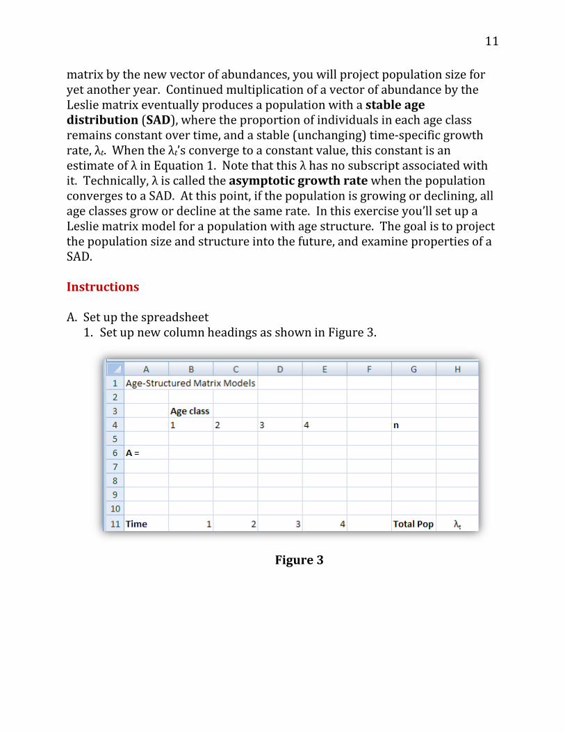
matrix by the new vector of abundances, you will project population size for yet another year. Continued multiplication of a vector of abundance by the Leslie matrix eventually produces a population with a stable age distribution (SAD), where the proportion of individuals in each age class remains constant over time, and a stable (unchanging) time-specific growth rate, λt. When the λt’s converge to a constant value, this constant is an estimate of λ in Equation 1. Note that this λ has no subscript associated with it. Technically, λ is called the asymptotic growth rate when the population converges to a SAD. At this point, if the population is growing or declining, all age classes grow or decline at the same rate. In this exercise you’ll set up a Leslie matrix model for a population with age structure. The goal is to project the population size and structure into the future, and examine properties of a SAD. Instructions A. Set up the spreadsheet

1. Set up new column headings as shown in Figure 3.

Figure 3

12

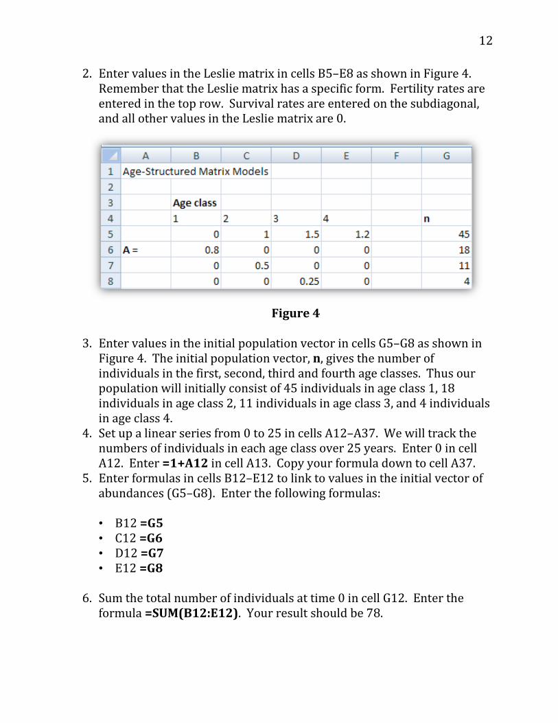
2. Enter values in the Leslie matrix in cells B5–E8 as shown in Figure 4. Remember that the Leslie matrix has a specific form. Fertility rates are entered in the top row. Survival rates are entered on the subdiagonal, and all other values in the Leslie matrix are 0.

Figure 4

3. Enter values in the initial population vector in cells G5–G8 as shown in Figure 4. The initial population vector, n, gives the number of individuals in the first, second, third and fourth age classes. Thus our population will initially consist of 45 individuals in age class 1, 18 individuals in age class 2, 11 individuals in age class 3, and 4 individuals in age class 4.

4. Set up a linear series from 0 to 25 in cells A12–A37. We will track the numbers of individuals in each age class over 25 years. Enter 0 in cell A12. Enter =1+A12 in cell A13. Copy your formula down to cell A37.

5. Enter formulas in cells B12–E12 to link to values in the initial vector of abundances (G5–G8). Enter the following formulas:

• B12 =G5 • C12 =G6 • D12 =G7 • E12 =G8

6. Sum the total number of individuals at time 0 in cell G12. Enter the

formula =SUM(B12:E12). Your result should be 78.

13

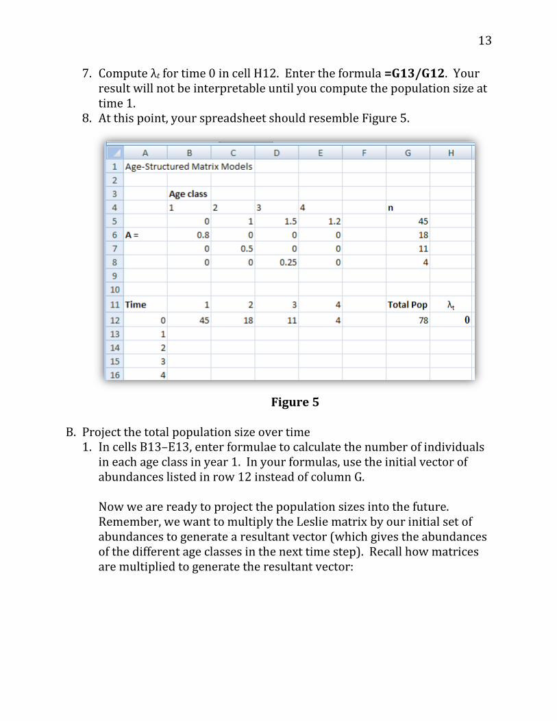
7. Compute λt for time 0 in cell H12. Enter the formula =G13/G12. Your result will not be interpretable until you compute the population size at time 1.

8. At this point, your spreadsheet should resemble Figure 5.

Figure 5 B. Project the total population size over time

1. In cells B13–E13, enter formulae to calculate the number of individuals in each age class in year 1. In your formulas, use the initial vector of abundances listed in row 12 instead of column G.

Now we are ready to project the population sizes into the future. Remember, we want to multiply the Leslie matrix by our initial set of abundances to generate a resultant vector (which gives the abundances of the different age classes in the next time step). Recall how matrices are multiplied to generate the resultant vector:

14

�

𝑎𝑎 𝑏𝑏 𝑐𝑐 𝑑𝑑𝑒𝑒 𝑓𝑓 𝑔𝑔 ℎ𝑖𝑖 𝑗𝑗 𝑘𝑘 𝑙𝑙𝑚𝑚 𝑛𝑛 𝑜𝑜 𝑝𝑝

�𝑥𝑥 �

𝑤𝑤𝑥𝑥𝑦𝑦𝑧𝑧

� = �

𝑎𝑎𝑤𝑤 + 𝑏𝑏𝑥𝑥 + 𝑐𝑐𝑦𝑦 + 𝑑𝑑𝑧𝑧𝑒𝑒𝑤𝑤 + 𝑓𝑓𝑥𝑥 + 𝑔𝑔𝑦𝑦 + ℎ𝑧𝑧𝑖𝑖𝑤𝑤 + 𝑗𝑗𝑥𝑥 + 𝑘𝑘𝑦𝑦 + 𝑙𝑙𝑧𝑧𝑚𝑚𝑤𝑤 + 𝑛𝑛𝑥𝑥 + 𝑜𝑜𝑦𝑦 + 𝑝𝑝𝑧𝑧

�

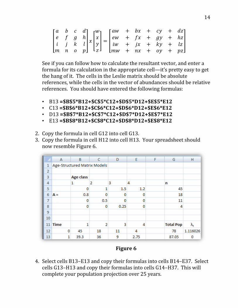
See if you can follow how to calculate the resultant vector, and enter a formula for its calculation in the appropriate cell—it’s pretty easy to get the hang of it. The cells in the Leslie matrix should be absolute references, while the cells in the vector of abundances should be relative references. You should have entered the following formulas:

• B13 =$B$5*B12+$C$5*C12+$D$5*D12+$E$5*E12 • C13 =$B$6*B12+$C$6*C12+$D$6*D12+$E$6*E12 • D13 =$B$7*B12+$C$7*C12+$D$7*D12+$E$7*E12 • E13 =$B$8*B12+$C$8*C12+$D$8*D12+$E$8*E12

2. Copy the formula in cell G12 into cell G13. 3. Copy the formula in cell H12 into cell H13. Your spreadsheet should

now resemble Figure 6.

Figure 6

4. Select cells B13–E13 and copy their formulas into cells B14–E37. Select cells G13–H13 and copy their formulas into cells G14–H37. This will complete your population projection over 25 years.

15

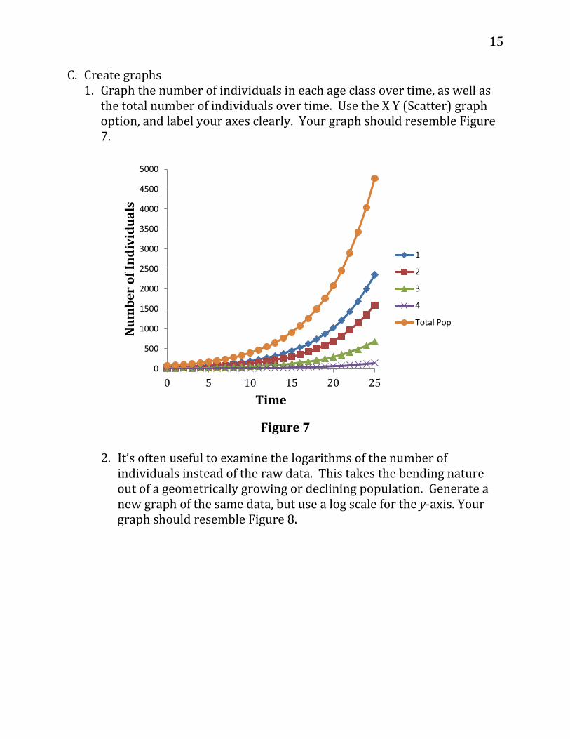
C. Create graphs 1. Graph the number of individuals in each age class over time, as well as

the total number of individuals over time. Use the X Y (Scatter) graph option, and label your axes clearly. Your graph should resemble Figure 7.

Figure 7

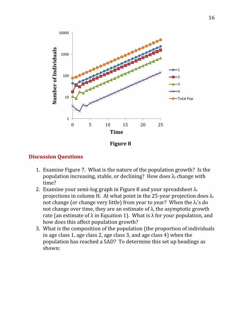
2. It’s often useful to examine the logarithms of the number of

individuals instead of the raw data. This takes the bending nature out of a geometrically growing or declining population. Generate a new graph of the same data, but use a log scale for the y-axis. Your graph should resemble Figure 8.

0

500

1000

1500

2000

2500

3000

3500

4000

4500

5000

0 5 10 15 20 25

Num

ber

of In

divi

dual

s

Time

1

2

3

4

Total Pop

16

Figure 8

Discussion Questions

1. Examine Figure 7. What is the nature of the population growth? Is the population increasing, stable, or declining? How does λt change with time?

2. Examine your semi-log graph in Figure 8 and your spreadsheet λt projections in column H. At what point in the 25-year projection does λt not change (or change very little) from year to year? When the λt’s do not change over time, they are an estimate of λ, the asymptotic growth rate (an estimate of λ in Equation 1). What is λ for your population, and how does this affect population growth?

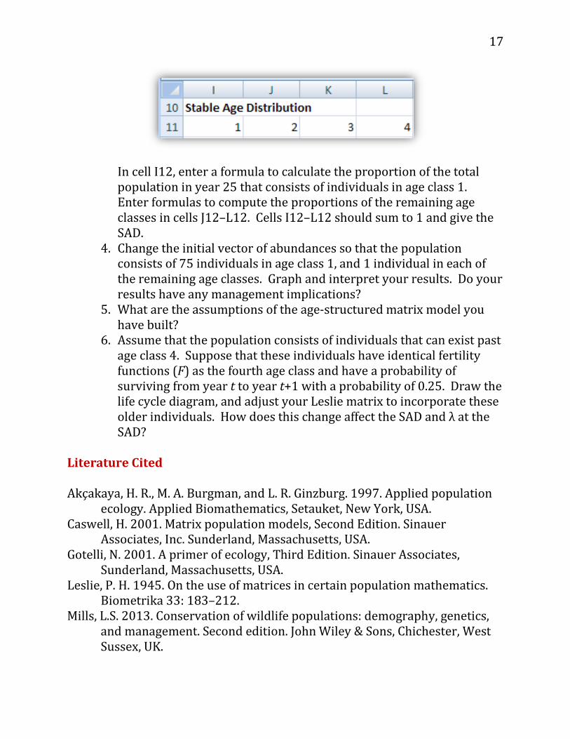
3. What is the composition of the population (the proportion of individuals in age class 1, age class 2, age class 3, and age class 4) when the population has reached a SAD? To determine this set up headings as shown:

1

10

100

1000

10000

0 5 10 15 20 25

Num

ber

of In

divi

dual

s

Time

1

2

3

4

Total Pop

17

In cell I12, enter a formula to calculate the proportion of the total population in year 25 that consists of individuals in age class 1. Enter formulas to compute the proportions of the remaining age classes in cells J12–L12. Cells I12–L12 should sum to 1 and give the SAD.

4. Change the initial vector of abundances so that the population consists of 75 individuals in age class 1, and 1 individual in each of the remaining age classes. Graph and interpret your results. Do your results have any management implications?

5. What are the assumptions of the age-structured matrix model you have built?

6. Assume that the population consists of individuals that can exist past age class 4. Suppose that these individuals have identical fertility functions (F) as the fourth age class and have a probability of surviving from year t to year t+1 with a probability of 0.25. Draw the life cycle diagram, and adjust your Leslie matrix to incorporate these older individuals. How does this change affect the SAD and λ at the SAD?

Literature Cited Akçakaya, H. R., M. A. Burgman, and L. R. Ginzburg. 1997. Applied population

ecology. Applied Biomathematics, Setauket, New York, USA. Caswell, H. 2001. Matrix population models, Second Edition. Sinauer

Associates, Inc. Sunderland, Massachusetts, USA. Gotelli, N. 2001. A primer of ecology, Third Edition. Sinauer Associates,

Sunderland, Massachusetts, USA. Leslie, P. H. 1945. On the use of matrices in certain population mathematics.

Biometrika 33: 183–212. Mills, L.S. 2013. Conservation of wildlife populations: demography, genetics,

and management. Second edition. John Wiley & Sons, Chichester, West Sussex, UK.

18

Acknowledgement This problem set was adapted from Exercise 13: Age-structured matrix models, pages 177-186 in Donovan, T. M. and C. Welden. 2002. Spreadsheet exercises in ecology and evolution. Sinauer Associates, Inc. Sunderland, MA, USA. This publication is available at http://www.uvm.edu/rsenr/vtcfwru/spreadsheets/?Page=ecologyevolution/EE13.htm. Your write-up should include the following: (1) a paragraph explaining the objectives of this problem set, and (2) your answers to the 5 discussion questions. Email me (whited@uamont.edu) your age-structured matrix spreadsheet model.