Embed Size (px)
Citation preview
ALADIN—An Algorithm for DistributedNon-Convex Optimization and Control
Boris Houska, Yuning Jiang, Janick Frasch,
Rien Quirynen, Dimitris Kouzoupis, Moritz Diehl
ShanghaiTech University, University of Magdeburg, University of Freiburg
1
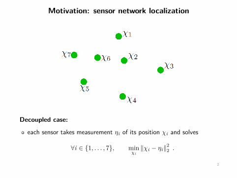
Motivation: sensor network localization
Decoupled case:
each sensor takes measurement ηi of its position χi and solves
∀i ∈ {1, . . . , 7}, minχi‖χi − ηi‖2
2 .
2
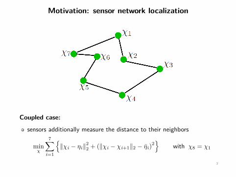
Motivation: sensor network localization
Coupled case:
sensors additionally measure the distance to their neighbors
minχ
7∑i=1
{‖χi − ηi‖2
2 + (‖χi − χi+1‖2 − η̄i)2}
with χ8 = χ1
3
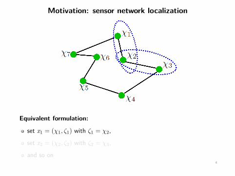
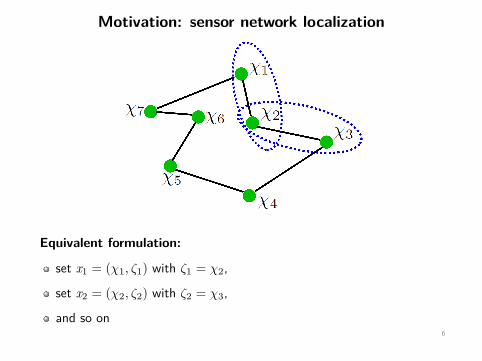
Motivation: sensor network localization
Equivalent formulation:
set x1 = (χ1, ζ1) with ζ1 = χ2,
set x2 = (χ2, ζ2) with ζ2 = χ3,
and so on4
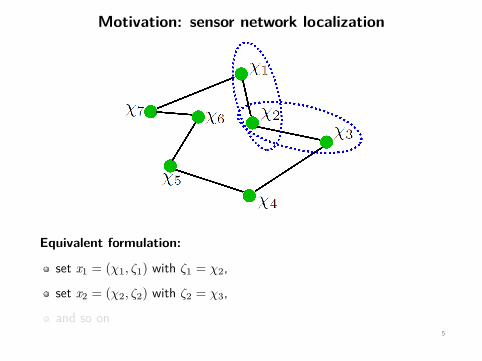
Motivation: sensor network localization
Equivalent formulation:
set x1 = (χ1, ζ1) with ζ1 = χ2,
set x2 = (χ2, ζ2) with ζ2 = χ3,
and so on5
Motivation: sensor network localization
Equivalent formulation:
set x1 = (χ1, ζ1) with ζ1 = χ2,
set x2 = (χ2, ζ2) with ζ2 = χ3,
and so on6
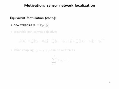
Motivation: sensor network localization
Equivalent formulation (cont.):
new variables xi = (χi , ζi)
separable non-convex objectives
fi(xi) = 12‖χi − ηi‖2
2 + 12‖ζi − ηi+1‖2
2 + 12 (‖χi − ζi‖2 − η̄i)2
affine coupling, ζi = χi+1, can be written as
7∑i=1
Aixi = 0 .
7
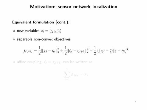
Motivation: sensor network localization
Equivalent formulation (cont.):
new variables xi = (χi , ζi)
separable non-convex objectives
fi(xi) = 12‖χi − ηi‖2
2 + 12‖ζi − ηi+1‖2
2 + 12 (‖χi − ζi‖2 − η̄i)2
affine coupling, ζi = χi+1, can be written as
7∑i=1
Aixi = 0 .
8
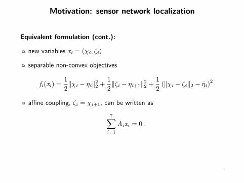
Motivation: sensor network localization
Equivalent formulation (cont.):
new variables xi = (χi , ζi)
separable non-convex objectives
fi(xi) = 12‖χi − ηi‖2
2 + 12‖ζi − ηi+1‖2
2 + 12 (‖χi − ζi‖2 − η̄i)2
affine coupling, ζi = χi+1, can be written as
7∑i=1
Aixi = 0 .
9
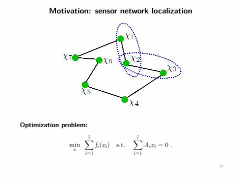
Motivation: sensor network localization
Optimization problem:
minx
7∑i=1
fi(xi) s.t.7∑
i=1Aixi = 0 .
10
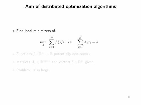
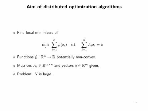
Aim of distributed optimization algorithms
Find local minimizers of
minx
N∑i=1
fi(xi) s.t.N∑
i=1Aixi = b
Functions fi : Rn → R potentially non-convex.
Matrices Ai ∈ Rm×n and vectors b ∈ Rm given.
Problem: N is large.
11
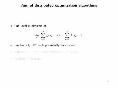
Aim of distributed optimization algorithms
Find local minimizers of
minx
N∑i=1
fi(xi) s.t.N∑
i=1Aixi = b
Functions fi : Rn → R potentially non-convex.
Matrices Ai ∈ Rm×n and vectors b ∈ Rm given.
Problem: N is large.
12
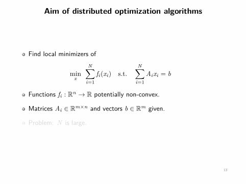
Aim of distributed optimization algorithms
Find local minimizers of
minx
N∑i=1
fi(xi) s.t.N∑
i=1Aixi = b
Functions fi : Rn → R potentially non-convex.
Matrices Ai ∈ Rm×n and vectors b ∈ Rm given.
Problem: N is large.
13
Aim of distributed optimization algorithms
Find local minimizers of
minx
N∑i=1
fi(xi) s.t.N∑
i=1Aixi = b
Functions fi : Rn → R potentially non-convex.
Matrices Ai ∈ Rm×n and vectors b ∈ Rm given.
Problem: N is large.
14
Overview
• Theory
- Distributed optimization algorithms
- ALADIN
• Applications
- Sensor network localization
- MPC with long horizons
15
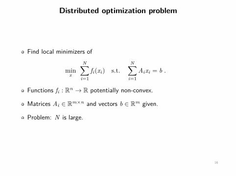
Distributed optimization problem
Find local minimizers of
minx
N∑i=1
fi(xi) s.t.N∑
i=1Aixi = b .
Functions fi : Rn → R potentially non-convex.
Matrices Ai ∈ Rm×n and vectors b ∈ Rm given.
Problem: N is large.
16
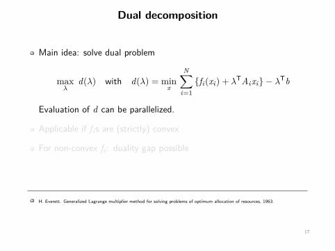
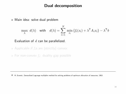
Dual decomposition
Main idea: solve dual problem
maxλ
d(λ) with d(λ) = minx
N∑i=1{fi(xi) + λTAixi} − λTb
Evaluation of d can be parallelized.
Applicable if fis are (strictly) convex
For non-convex fi : duality gap possible
H. Everett. Generalized Lagrange multiplier method for solving problems of optimum allocation of resources, 1963.
17
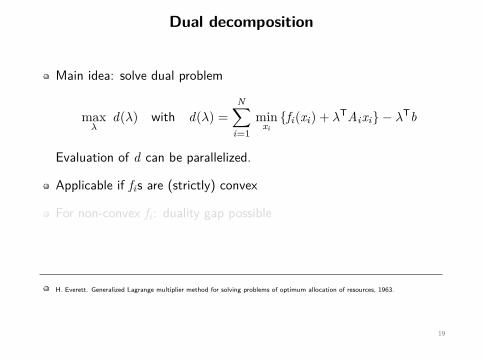
Dual decomposition
Main idea: solve dual problem
maxλ
d(λ) with d(λ) =N∑
i=1min
xi{fi(xi) + λTAixi} − λTb
Evaluation of d can be parallelized.
Applicable if fis are (strictly) convex
For non-convex fi : duality gap possible
H. Everett. Generalized Lagrange multiplier method for solving problems of optimum allocation of resources, 1963.
18
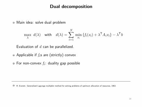
Dual decomposition
Main idea: solve dual problem
maxλ
d(λ) with d(λ) =N∑
i=1min
xi{fi(xi) + λTAixi} − λTb
Evaluation of d can be parallelized.
Applicable if fis are (strictly) convex
For non-convex fi : duality gap possible
H. Everett. Generalized Lagrange multiplier method for solving problems of optimum allocation of resources, 1963.
19
Dual decomposition
Main idea: solve dual problem
maxλ
d(λ) with d(λ) =N∑
i=1min
xi{fi(xi) + λTAixi} − λTb
Evaluation of d can be parallelized.
Applicable if fis are (strictly) convex
For non-convex fi : duality gap possible
H. Everett. Generalized Lagrange multiplier method for solving problems of optimum allocation of resources, 1963.
20
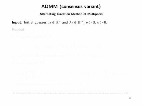
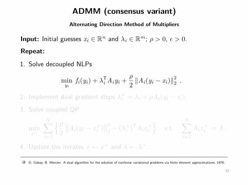
ADMM (consensus variant)Alternating Direction Method of Multipliers
Input: Initial guesses xi ∈ Rn and λi ∈ Rm; ρ > 0, ε > 0.
Repeat:
1. Solve decoupled NLPs
minyi
fi(yi) + λTi Aiyi + ρ
2 ‖Ai(yi − xi)‖22 .
2. Implement dual gradient steps λ+i = λi + ρAi(yi − xi).
3. Solve coupled QP
minx+
N∑i=1
{ρ2∥∥Ai(yi − x+
i )∥∥2
2 − (λ+i )TAix+
i
}s.t.
N∑i=1
Aix+i = b .
4. Update the iterates x ← x+ and λ← λ+.
D. Gabay, B. Mercier. A dual algorithm for the solution of nonlinear variational problems via finite element approximations, 1976.
21
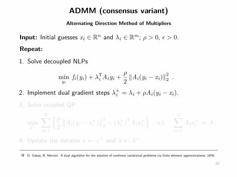
ADMM (consensus variant)Alternating Direction Method of Multipliers
Input: Initial guesses xi ∈ Rn and λi ∈ Rm; ρ > 0, ε > 0.
Repeat:
1. Solve decoupled NLPs
minyi
fi(yi) + λTi Aiyi + ρ
2 ‖Ai(yi − xi)‖22 .
2. Implement dual gradient steps λ+i = λi + ρAi(yi − xi).
3. Solve coupled QP
minx+
N∑i=1
{ρ2∥∥Ai(yi − x+
i )∥∥2
2 − (λ+i )TAix+
i
}s.t.
N∑i=1
Aix+i = b .
4. Update the iterates x ← x+ and λ← λ+.
D. Gabay, B. Mercier. A dual algorithm for the solution of nonlinear variational problems via finite element approximations, 1976.
22
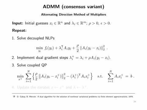
ADMM (consensus variant)Alternating Direction Method of Multipliers
Input: Initial guesses xi ∈ Rn and λi ∈ Rm; ρ > 0, ε > 0.
Repeat:
1. Solve decoupled NLPs
minyi
fi(yi) + λTi Aiyi + ρ
2 ‖Ai(yi − xi)‖22 .
2. Implement dual gradient steps λ+i = λi + ρAi(yi − xi).
3. Solve coupled QP
minx+
N∑i=1
{ρ2∥∥Ai(yi − x+
i )∥∥2
2 − (λ+i )TAix+
i
}s.t.
N∑i=1
Aix+i = b .
4. Update the iterates x ← x+ and λ← λ+.
D. Gabay, B. Mercier. A dual algorithm for the solution of nonlinear variational problems via finite element approximations, 1976.
23
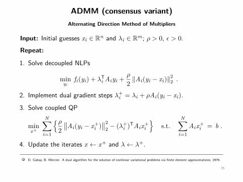
ADMM (consensus variant)Alternating Direction Method of Multipliers
Input: Initial guesses xi ∈ Rn and λi ∈ Rm; ρ > 0, ε > 0.
Repeat:
1. Solve decoupled NLPs
minyi
fi(yi) + λTi Aiyi + ρ
2 ‖Ai(yi − xi)‖22 .
2. Implement dual gradient steps λ+i = λi + ρAi(yi − xi).
3. Solve coupled QP
minx+
N∑i=1
{ρ2∥∥Ai(yi − x+
i )∥∥2
2 − (λ+i )TAix+
i
}s.t.
N∑i=1
Aix+i = b .
4. Update the iterates x ← x+ and λ← λ+.
D. Gabay, B. Mercier. A dual algorithm for the solution of nonlinear variational problems via finite element approximations, 1976.
24
ADMM (consensus variant)Alternating Direction Method of Multipliers
Input: Initial guesses xi ∈ Rn and λi ∈ Rm; ρ > 0, ε > 0.
Repeat:
1. Solve decoupled NLPs
minyi
fi(yi) + λTi Aiyi + ρ
2 ‖Ai(yi − xi)‖22 .
2. Implement dual gradient steps λ+i = λi + ρAi(yi − xi).
3. Solve coupled QP
minx+
N∑i=1
{ρ2∥∥Ai(yi − x+
i )∥∥2
2 − (λ+i )TAix+
i
}s.t.
N∑i=1
Aix+i = b .
4. Update the iterates x ← x+ and λ← λ+.
D. Gabay, B. Mercier. A dual algorithm for the solution of nonlinear variational problems via finite element approximations, 1976.
25
Limitations of ADMM
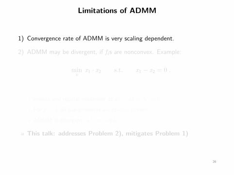
1) Convergence rate of ADMM is very scaling dependent.
2) ADMM may be divergent, if fis are nonconvex. Example:
minx
x1 · x2 s.t. x1 − x2 = 0 .
unique and regular minimizer at x∗1 = x∗
2 = λ∗ = 0.
For ρ = 34 all sub-problems are strictly convex.
ADMM is divergent; λ+ = −2λ.
This talk: addresses Problem 2), mitigates Problem 1)
26

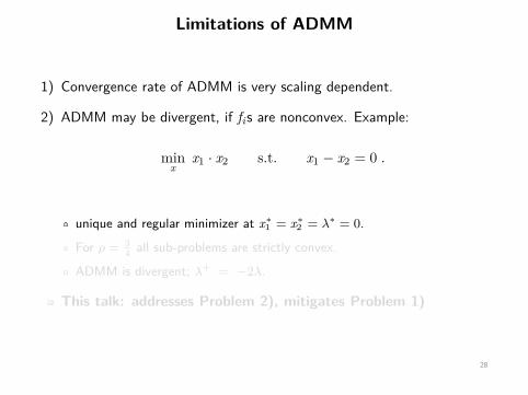
Limitations of ADMM
1) Convergence rate of ADMM is very scaling dependent.
2) ADMM may be divergent, if fis are nonconvex. Example:
minx
x1 · x2 s.t. x1 − x2 = 0 .
unique and regular minimizer at x∗1 = x∗
2 = λ∗ = 0.
For ρ = 34 all sub-problems are strictly convex.
ADMM is divergent; λ+ = −2λ.
This talk: addresses Problem 2), mitigates Problem 1)
27
Limitations of ADMM
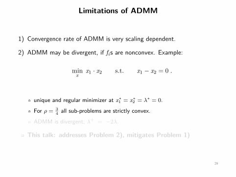
1) Convergence rate of ADMM is very scaling dependent.
2) ADMM may be divergent, if fis are nonconvex. Example:
minx
x1 · x2 s.t. x1 − x2 = 0 .
unique and regular minimizer at x∗1 = x∗
2 = λ∗ = 0.
For ρ = 34 all sub-problems are strictly convex.
ADMM is divergent; λ+ = −2λ.
This talk: addresses Problem 2), mitigates Problem 1)
28
Limitations of ADMM
1) Convergence rate of ADMM is very scaling dependent.
2) ADMM may be divergent, if fis are nonconvex. Example:
minx
x1 · x2 s.t. x1 − x2 = 0 .
unique and regular minimizer at x∗1 = x∗
2 = λ∗ = 0.
For ρ = 34 all sub-problems are strictly convex.
ADMM is divergent; λ+ = −2λ.
This talk: addresses Problem 2), mitigates Problem 1)
29
Limitations of ADMM
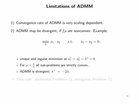
1) Convergence rate of ADMM is very scaling dependent.
2) ADMM may be divergent, if fis are nonconvex. Example:
minx
x1 · x2 s.t. x1 − x2 = 0 .
unique and regular minimizer at x∗1 = x∗
2 = λ∗ = 0.
For ρ = 34 all sub-problems are strictly convex.
ADMM is divergent; λ+ = −2λ.
This talk: addresses Problem 2), mitigates Problem 1)
30
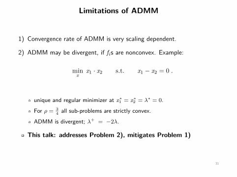
Limitations of ADMM
1) Convergence rate of ADMM is very scaling dependent.
2) ADMM may be divergent, if fis are nonconvex. Example:
minx
x1 · x2 s.t. x1 − x2 = 0 .
unique and regular minimizer at x∗1 = x∗
2 = λ∗ = 0.
For ρ = 34 all sub-problems are strictly convex.
ADMM is divergent; λ+ = −2λ.
This talk: addresses Problem 2), mitigates Problem 1)
31
Overview
• Theory
- Distributed optimization algorithms
- ALADIN
• Applications
- Sensor network localization
- MPC with long horizons
32
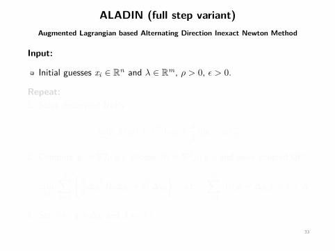
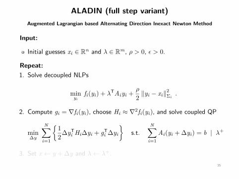
ALADIN (full step variant)Augmented Lagrangian based Alternating Direction Inexact Newton Method
Input:
Initial guesses xi ∈ Rn and λ ∈ Rm, ρ > 0, ε > 0.
Repeat:1. Solve decoupled NLPs
minyi
fi(yi) + λTAiyi + ρ
2 ‖yi − xi‖2Σi
.
2. Compute gi = ∇fi(yi), choose Hi ≈ ∇2fi(yi), and solve coupled QP
min∆y
N∑i=1
{12∆yT
i Hi∆yi + gTi ∆yi
}s.t.
N∑i=1
Ai(yi + ∆yi) = b | λ+
3. Set x ← y + ∆y and λ← λ+.33
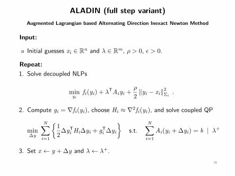
ALADIN (full step variant)Augmented Lagrangian based Alternating Direction Inexact Newton Method
Input:
Initial guesses xi ∈ Rn and λ ∈ Rm, ρ > 0, ε > 0.
Repeat:1. Solve decoupled NLPs
minyi
fi(yi) + λTAiyi + ρ
2 ‖yi − xi‖2Σi
.
2. Compute gi = ∇fi(yi), choose Hi ≈ ∇2fi(yi), and solve coupled QP
min∆y
N∑i=1
{12∆yT
i Hi∆yi + gTi ∆yi
}s.t.
N∑i=1
Ai(yi + ∆yi) = b | λ+
3. Set x ← y + ∆y and λ← λ+.34
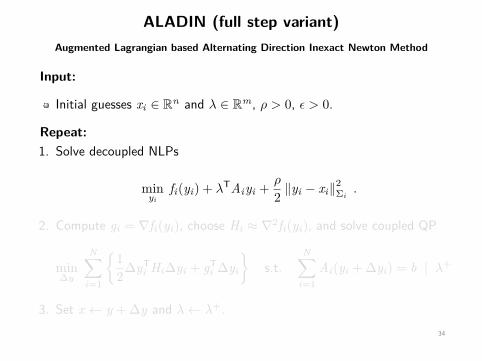
ALADIN (full step variant)Augmented Lagrangian based Alternating Direction Inexact Newton Method
Input:
Initial guesses xi ∈ Rn and λ ∈ Rm, ρ > 0, ε > 0.
Repeat:1. Solve decoupled NLPs
minyi
fi(yi) + λTAiyi + ρ
2 ‖yi − xi‖2Σi
.
2. Compute gi = ∇fi(yi), choose Hi ≈ ∇2fi(yi), and solve coupled QP
min∆y
N∑i=1
{12∆yT
i Hi∆yi + gTi ∆yi
}s.t.
N∑i=1
Ai(yi + ∆yi) = b | λ+
3. Set x ← y + ∆y and λ← λ+.35
ALADIN (full step variant)Augmented Lagrangian based Alternating Direction Inexact Newton Method
Input:
Initial guesses xi ∈ Rn and λ ∈ Rm, ρ > 0, ε > 0.
Repeat:1. Solve decoupled NLPs
minyi
fi(yi) + λTAiyi + ρ
2 ‖yi − xi‖2Σi
.
2. Compute gi = ∇fi(yi), choose Hi ≈ ∇2fi(yi), and solve coupled QP
min∆y
N∑i=1
{12∆yT
i Hi∆yi + gTi ∆yi
}s.t.
N∑i=1
Ai(yi + ∆yi) = b | λ+
3. Set x ← y + ∆y and λ← λ+.36
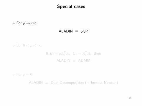
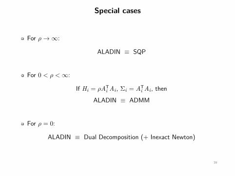
Special cases
For ρ→∞:
ALADIN ≡ SQP
For 0 < ρ <∞:
If Hi = ρATi Ai , Σi = AT
i Ai , then
ALADIN ≡ ADMM
For ρ = 0:
ALADIN ≡ Dual Decomposition (+ Inexact Newton)
37
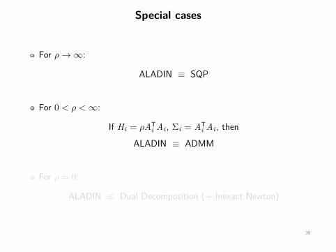
Special cases
For ρ→∞:
ALADIN ≡ SQP
For 0 < ρ <∞:
If Hi = ρATi Ai , Σi = AT
i Ai , then
ALADIN ≡ ADMM
For ρ = 0:
ALADIN ≡ Dual Decomposition (+ Inexact Newton)
38
Special cases
For ρ→∞:
ALADIN ≡ SQP
For 0 < ρ <∞:
If Hi = ρATi Ai , Σi = AT
i Ai , then
ALADIN ≡ ADMM
For ρ = 0:
ALADIN ≡ Dual Decomposition (+ Inexact Newton)
39
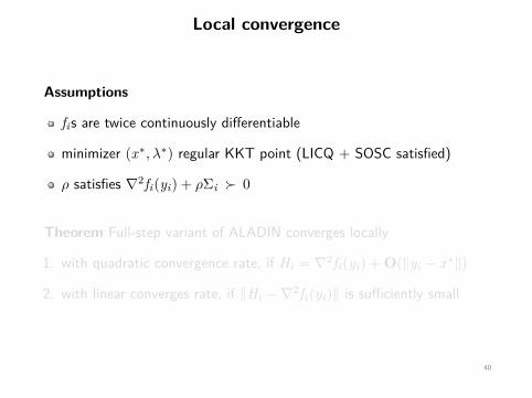
Local convergence
Assumptions
fis are twice continuously differentiable
minimizer (x∗, λ∗) regular KKT point (LICQ + SOSC satisfied)
ρ satisfies ∇2fi(yi) + ρΣi � 0
Theorem Full-step variant of ALADIN converges locally
1. with quadratic convergence rate, if Hi = ∇2fi(yi) + O(‖yi − x∗‖)
2. with linear converges rate, if ‖Hi −∇2fi(yi)‖ is sufficiently small
40
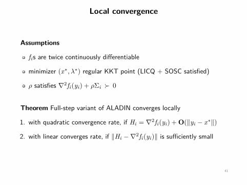
Local convergence
Assumptions
fis are twice continuously differentiable
minimizer (x∗, λ∗) regular KKT point (LICQ + SOSC satisfied)
ρ satisfies ∇2fi(yi) + ρΣi � 0
Theorem Full-step variant of ALADIN converges locally
1. with quadratic convergence rate, if Hi = ∇2fi(yi) + O(‖yi − x∗‖)
2. with linear converges rate, if ‖Hi −∇2fi(yi)‖ is sufficiently small
41
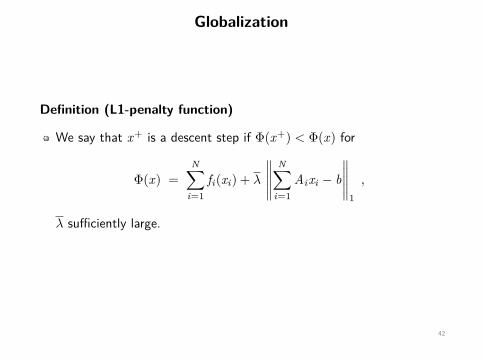
Globalization
Definition (L1-penalty function)
We say that x+ is a descent step if Φ(x+) < Φ(x) for
Φ(x) =N∑
i=1fi(xi) + λ
∥∥∥∥∥N∑
i=1Aixi − b
∥∥∥∥∥1
,
λ sufficiently large.
42
GlobalizationRough sketch:
As long as ∇2fi(xi) + ρΣi � 0 the proximal objectives
f̃i(yi) = fi(yi) + ρ
2 ‖yi − xi‖2Σi
are strictly convex in a neighborhood of the current primal iterates xi .
If we don’t update x, y can be enforced to converge to the solution z
of the convex auxiliary problem
minz
N∑i=1
f̃i(zi) s.t.N∑
i=1Aizi = b .
Strategy: if x+ is not a descent direction, we skip the primal update
until y is a descent and set x+ = y (similar to proximal methods)
This strategy leads to a globalization routine for ALADIN if Hi � 0.43
GlobalizationRough sketch:
As long as ∇2fi(xi) + ρΣi � 0 the proximal objectives
f̃i(yi) = fi(yi) + ρ
2 ‖yi − xi‖2Σi
are strictly convex in a neighborhood of the current primal iterates xi .
If we don’t update x, y can be enforced to converge to the solution z
of the convex auxiliary problem
minz
N∑i=1
f̃i(zi) s.t.N∑
i=1Aizi = b .
Strategy: if x+ is not a descent direction, we skip the primal update
until y is a descent and set x+ = y (similar to proximal methods)
This strategy leads to a globalization routine for ALADIN if Hi � 0.44
GlobalizationRough sketch:
As long as ∇2fi(xi) + ρΣi � 0 the proximal objectives
f̃i(yi) = fi(yi) + ρ
2 ‖yi − xi‖2Σi
are strictly convex in a neighborhood of the current primal iterates xi .
If we don’t update x, y can be enforced to converge to the solution z
of the convex auxiliary problem
minz
N∑i=1
f̃i(zi) s.t.N∑
i=1Aizi = b .
Strategy: if x+ is not a descent direction, we skip the primal update
until y is a descent and set x+ = y (similar to proximal methods)
This strategy leads to a globalization routine for ALADIN if Hi � 0.45
GlobalizationRough sketch:
As long as ∇2fi(xi) + ρΣi � 0 the proximal objectives
f̃i(yi) = fi(yi) + ρ
2 ‖yi − xi‖2Σi
are strictly convex in a neighborhood of the current primal iterates xi .
If we don’t update x, y can be enforced to converge to the solution z
of the convex auxiliary problem
minz
N∑i=1
f̃i(zi) s.t.N∑
i=1Aizi = b .
Strategy: if x+ is not a descent direction, we skip the primal update
until y is a descent and set x+ = y (similar to proximal methods)
This strategy leads to a globalization routine for ALADIN if Hi � 0.46
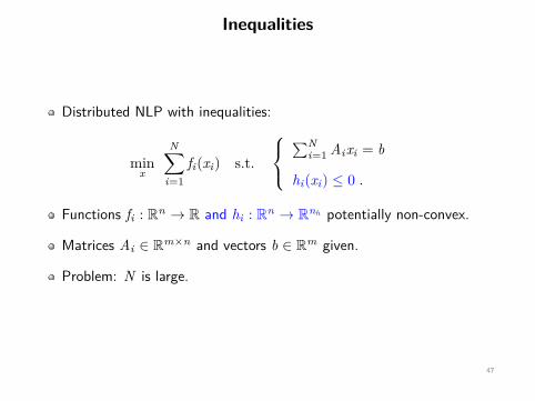
Inequalities
Distributed NLP with inequalities:
minx
N∑i=1
fi(xi) s.t.
∑N
i=1 Aixi = b
hi(xi) ≤ 0 .
Functions fi : Rn → R and hi : Rn → Rnh potentially non-convex.
Matrices Ai ∈ Rm×n and vectors b ∈ Rm given.
Problem: N is large.
47
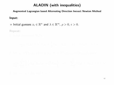
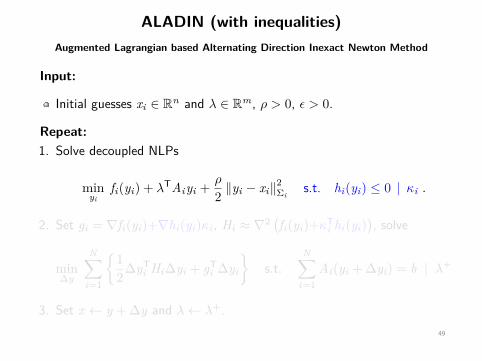
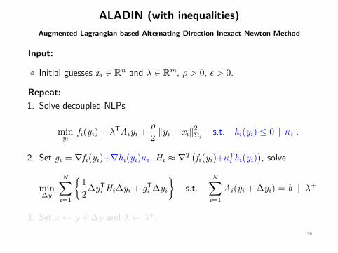
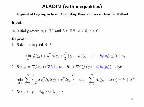
ALADIN (with inequalities)Augmented Lagrangian based Alternating Direction Inexact Newton Method
Input:
Initial guesses xi ∈ Rn and λ ∈ Rm, ρ > 0, ε > 0.
Repeat:1. Solve decoupled NLPs
minyi
fi(yi) + λTAiyi + ρ
2 ‖yi − xi‖2Σi
s.t. hi(yi) ≤ 0 | κi .
2. Set gi = ∇fi(yi)+∇hi(yi)κi , Hi ≈ ∇2 (fi(yi)+κTi hi(yi)), solve
min∆y
N∑i=1
{12∆yT
i Hi∆yi + gTi ∆yi
}s.t.
N∑i=1
Ai(yi + ∆yi) = b | λ+
3. Set x ← y + ∆y and λ← λ+.48
ALADIN (with inequalities)Augmented Lagrangian based Alternating Direction Inexact Newton Method
Input:
Initial guesses xi ∈ Rn and λ ∈ Rm, ρ > 0, ε > 0.
Repeat:1. Solve decoupled NLPs
minyi
fi(yi) + λTAiyi + ρ
2 ‖yi − xi‖2Σi
s.t. hi(yi) ≤ 0 | κi .
2. Set gi = ∇fi(yi)+∇hi(yi)κi , Hi ≈ ∇2 (fi(yi)+κTi hi(yi)), solve
min∆y
N∑i=1
{12∆yT
i Hi∆yi + gTi ∆yi
}s.t.
N∑i=1
Ai(yi + ∆yi) = b | λ+
3. Set x ← y + ∆y and λ← λ+.49
ALADIN (with inequalities)Augmented Lagrangian based Alternating Direction Inexact Newton Method
Input:
Initial guesses xi ∈ Rn and λ ∈ Rm, ρ > 0, ε > 0.
Repeat:1. Solve decoupled NLPs
minyi
fi(yi) + λTAiyi + ρ
2 ‖yi − xi‖2Σi
s.t. hi(yi) ≤ 0 | κi .
2. Set gi = ∇fi(yi)+∇hi(yi)κi , Hi ≈ ∇2 (fi(yi)+κTi hi(yi)), solve
min∆y
N∑i=1
{12∆yT
i Hi∆yi + gTi ∆yi
}s.t.
N∑i=1
Ai(yi + ∆yi) = b | λ+
3. Set x ← y + ∆y and λ← λ+.50
ALADIN (with inequalities)Augmented Lagrangian based Alternating Direction Inexact Newton Method
Input:
Initial guesses xi ∈ Rn and λ ∈ Rm, ρ > 0, ε > 0.
Repeat:1. Solve decoupled NLPs
minyi
fi(yi) + λTAiyi + ρ
2 ‖yi − xi‖2Σi
s.t. hi(yi) ≤ 0 | κi .
2. Set gi = ∇fi(yi)+∇hi(yi)κi , Hi ≈ ∇2 (fi(yi)+κTi hi(yi)), solve
min∆y
N∑i=1
{12∆yT
i Hi∆yi + gTi ∆yi
}s.t.
N∑i=1
Ai(yi + ∆yi) = b | λ+
3. Set x ← y + ∆y and λ← λ+.51
ALADIN (with inequalities)Augmented Lagrangian based Alternating Direction Inexact Newton Method
Remarks:
If approximation Ci ≈ C ∗i = ∇hi(yi) is available, solve QP
min∆y,s∑N
i=1{ 1
2 ∆yTi Hi∆yi + gTi ∆yi
}+ λTs + µ
2 ‖s‖22
s.t.
∑N
i=1 Ai (yi + ∆yi) = b + s∣∣∣ λQP
Ci∆yi = 0 , i ∈ {1, . . . ,N} .
with gi = ∇fi(yi) + (C ∗i − Ci)Tκi and µ > 0 instead.
If Hi and Ci constant, pre-compute matrix decompositions
52
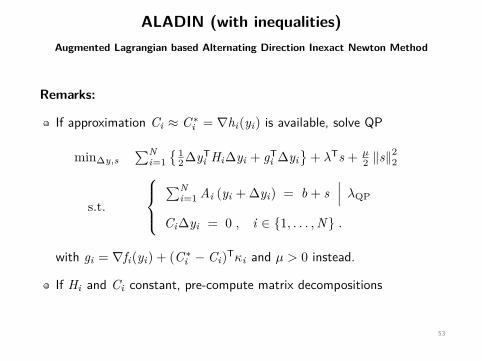
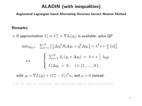
ALADIN (with inequalities)Augmented Lagrangian based Alternating Direction Inexact Newton Method
Remarks:
If approximation Ci ≈ C ∗i = ∇hi(yi) is available, solve QP
min∆y,s∑N
i=1{ 1
2 ∆yTi Hi∆yi + gTi ∆yi
}+ λTs + µ
2 ‖s‖22
s.t.
∑N
i=1 Ai (yi + ∆yi) = b + s∣∣∣ λQP
Ci∆yi = 0 , i ∈ {1, . . . ,N} .
with gi = ∇fi(yi) + (C ∗i − Ci)Tκi and µ > 0 instead.
If Hi and Ci constant, pre-compute matrix decompositions
53
Overview
• Theory
- Distributed Optimization Algorithms
- ALADIN
• Applications
- Sensor network localization
- MPC with long horizons
54

Sensor network localization
Case study:
25000 sensors measure positions and distances in a graph
additional inequality constraints, ‖χi − ηi‖2 ≤ σ̄, remove outliers.55
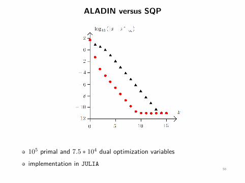
ALADIN versus SQP
105 primal and 7.5 ∗ 104 dual optimization variables
implementation in JULIA56
Overview
• Theory
- Distributed Optimization Algorithms
- ALADIN
• Applications
- Sensor network localization
- MPC with long horizons
57
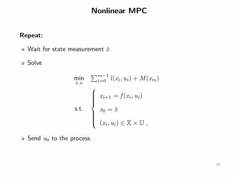
Nonlinear MPC
Repeat:
Wait for state measurement x̂.
Solve
minx,u
∑m−1i=0 l(xi , ui) + M (xm)
s.t.
xi+1 = f (xi , ui)
x0 = x̂
(xi , ui) ∈ X× U ,
Send u0 to the process.
58
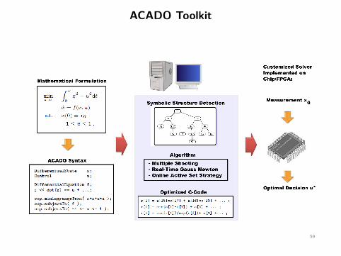
ACADO Toolkit
59
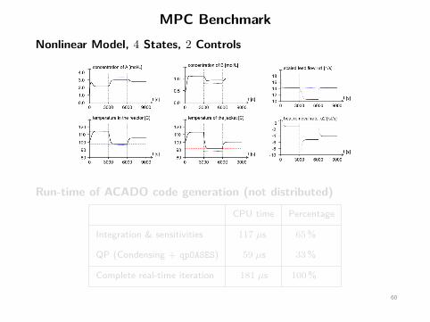
MPC BenchmarkNonlinear Model, 4 States, 2 Controls
Run-time of ACADO code generation (not distributed)
CPU time Percentage
Integration & sensitivities 117 µs 65%
QP (Condensing + qpOASES) 59 µs 33%
Complete real-time iteration 181 µs 100%
60
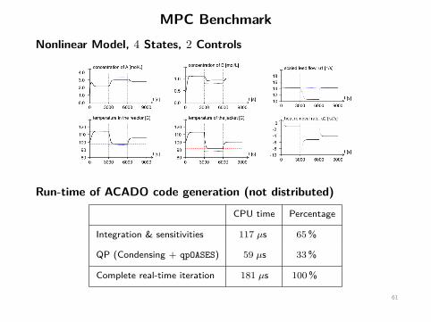
MPC BenchmarkNonlinear Model, 4 States, 2 Controls
Run-time of ACADO code generation (not distributed)
CPU time Percentage
Integration & sensitivities 117 µs 65%
QP (Condensing + qpOASES) 59 µs 33%
Complete real-time iteration 181 µs 100%
61
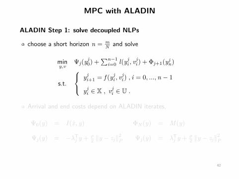
MPC with ALADIN
ALADIN Step 1: solve decoupled NLPs
choose a short horizon n = mN and solve
miny,v
Ψj(yj0) +
∑n−1i=0 l(yj
i , vji ) + Φj+1(yj
n)
s.t.
yji+1 = f (yj
i , vji ) , i = 0, ...,n − 1
yji ∈ X , vj
i ∈ U .
Arrival and end costs depend on ALADIN iterates,
Ψ0(y) = I (x̂, y) ΦN (y) = M (y)
Ψj(y) = −λTj y + ρ2 ‖y − zj‖2
P Ψj(y) = λTj y + ρ2 ‖y − zj‖2
P
62
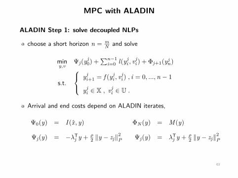
MPC with ALADIN
ALADIN Step 1: solve decoupled NLPs
choose a short horizon n = mN and solve
miny,v
Ψj(yj0) +
∑n−1i=0 l(yj
i , vji ) + Φj+1(yj
n)
s.t.
yji+1 = f (yj
i , vji ) , i = 0, ...,n − 1
yji ∈ X , vj
i ∈ U .
Arrival and end costs depend on ALADIN iterates,
Ψ0(y) = I (x̂, y) ΦN (y) = M (y)
Ψj(y) = −λTj y + ρ2 ‖y − zj‖2
P Ψj(y) = λTj y + ρ2 ‖y − zj‖2
P
63
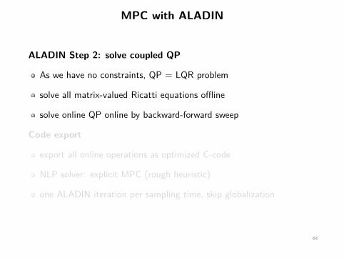
MPC with ALADIN
ALADIN Step 2: solve coupled QP
As we have no constraints, QP = LQR problem
solve all matrix-valued Ricatti equations offline
solve online QP online by backward-forward sweep
Code export
export all online operations as optimized C-code
NLP solver: explicit MPC (rough heuristic)
one ALADIN iteration per sampling time, skip globalization
64
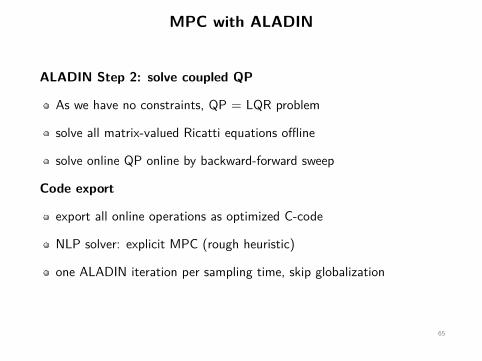
MPC with ALADIN
ALADIN Step 2: solve coupled QP
As we have no constraints, QP = LQR problem
solve all matrix-valued Ricatti equations offline
solve online QP online by backward-forward sweep
Code export
export all online operations as optimized C-code
NLP solver: explicit MPC (rough heuristic)
one ALADIN iteration per sampling time, skip globalization
65
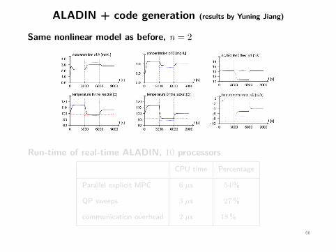
ALADIN + code generation (results by Yuning Jiang)
Same nonlinear model as before, n = 2
Run-time of real-time ALADIN, 10 processorsCPU time Percentage
Parallel explicit MPC 6 µs 54%
QP sweeps 3 µs 27%
communication overhead 2 µs 18%
66
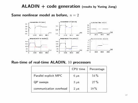
ALADIN + code generation (results by Yuning Jiang)
Same nonlinear model as before, n = 2
Run-time of real-time ALADIN, 10 processorsCPU time Percentage
Parallel explicit MPC 6 µs 54%
QP sweeps 3 µs 27%
communication overhead 2 µs 18%
67
Conclusions
ALADIN Theory
can solve nonconvex distributed optimization problems,
minx
N∑i=1
fi(xi) s.t.N∑
i=1Aixi = b ,
to local optimality.
contains SQP, ADMM, and Dual Decomposition as special case
local convergence analysis similar to SQP; globalization possible
68
Conclusions
ALADIN Theory
can solve nonconvex distributed optimization problems,
minx
N∑i=1
fi(xi) s.t.N∑
i=1Aixi = b ,
to local optimality.
contains SQP, ADMM, and Dual Decomposition as special case
local convergence analysis similar to SQP; globalization possible
69
Conclusions
ALADIN Theory
can solve nonconvex distributed optimization problems,
minx
N∑i=1
fi(xi) s.t.N∑
i=1Aixi = b ,
to local optimality.
contains SQP, ADMM, and Dual Decomposition as special case
local convergence analysis similar to SQP; globalization possible
70
Conclusions
ALADIN Applications
large-scale distributed sensor network:
ALADIN outperforms SQP and ADMM
small-scale embedded MPC:
ALADIN can be used to alternate between explicit & online MPC
71
Conclusions
ALADIN Applications
large-scale distributed sensor network:
ALADIN outperforms SQP and ADMM
small-scale embedded MPC:
ALADIN can be used to alternate between explicit & online MPC
72
References
• B. Houska, J. Frasch, M. Diehl. An Augmented Lagrangian Based Algorithm for
Distributed Non-Convex Optimization. SIOPT, 2016.
• D. Kouzoupis, R. Quirynen, B. Houska, M. Diehl. A block based ALADIN scheme
for highly parallelizable direct optimal control. ACC, 2016.
73