Embed Size (px)
Citation preview
Roman Dementiev
Algorithm Engineeringfor Large Data Sets
SA
RA V I E N
SI
S
UN
I VE R S I T
AS
Dissertation zur Erlangung des Grades
des Doktors der Ingenieurwissenschaften (Dr.-Ing.)der Naturwissenschaftlich-Technischen Fakultaten
der Universitat des Saarlandes
Saarbrucken, 2006
II
Tag des Kolloqiums/Day of the colloquium: 1. Dez 2006 / 1 Dec 2006
Dekan/Dean: Prof. Dr. Thorsten Herfet
Gutachter/Reviewers: Prof. Dr. rer. nat. Peter SandersProf. Dr.-Ing. Gerhard Weikum
Prufungsausschuss/Board of examiners: Prof. Dr. rer. nat. Peter Sanders
Prof. Dr.-Ing. Gerhard WeikumProf. Dr. Kurt Mehlhorn
Dr.-Ing. Ulrich Carsten Meyer
III
Short Abstract
In recent years, the development of theoretically I/O-efficient algorithms anddata structures has received considerable attention. However, much less hasbeen done to evaluate their performance, in particular with parallel disks orwhen running on large inputs with sizes that really require external mem-ory. This thesis presents the software library Stxxl that enables practice-oriented experimentation with huge data sets. Stxxl is an implementationof the C++ standard template library STL for external memory computa-tions. It supports parallel disks, overlapping between I/O and computationand it is the first external memory algorithm library that supports the pipelin-ing technique that can save more than half of the I/Os. We engineer practicalI/O-efficient algorithms and their Stxxl implementations for the followingproblems: (minimum) spanning forests, connected components, breadth-firstsearch decompositions, suffix array construction, computation of social net-work analysis metrics and graph coloring. The performance of the Stxxl
and its applications is evaluated on many synthetic and real-world inputs.
Kurze Zusammenfassung
In den vergangenen Jahren wurde der Entwicklung von theoretisch I/O-effizienten Algorithmen und Datenstrukturen viel Aufmerksamkeit gewid-met. Im Gegensatz dazu wurde viel weniger dafur getan, ihre Leistung inder Praxis auszuwerten, vor allem in Bezug auf parallele Festplatten oderdie Verarbeitung großer Datenmengen, die externen Speicher wirklich ver-langen. Aus diesem Grunde ermoglicht die im Rahmen dieser Doktorar-beit entwickelte Software-Bibliothek Stxxl nun das praxisorientierte Ex-perimentieren mit großen Datensatzen. Stxxl ist eine Implementierungder C++ Standard Template Library (STL) fur Rechenvorgange im exter-nen Speicher. Sie uberlagert I/O und Berechnung und unterstutzt paralleleFestplatten. Auch ist sie die erste Algorithmen-Bibliothek fur externe Spei-cher, die das Pipelining-Verfahren unterstutzt, welches mehr als die Halfteder I/Os einsparen kann. Praktische I/O-effiziente Algorithmen und ihreStxxl-Implementierungen wurden fur die folgenden Problemstellungen ent-wickelt: (minimale) spannende Baume, Zusammenhangskomponenten, Brei-tensuche, Konstruktion von Suffix-Tabellen, Berechnung von Metriken fursoziale Netzwerk-Analyse und Graphfarbung. Zur Leistungsuberprufung sindStxxl und ihre Applikationen mit vielen synthetischen, aber auch realenEingaben getestet worden.
IV
Abstract
Massive data sets arise naturally in many domains: geographic informationsystems, computer graphics, database systems, telecommunication billingsystems [Hum02], network analysis [DLL+06], and scientific computing[Moo00]. Applications working in those domains have to process terabytesof data. However, the internal memories of computers can only keep a smallfraction of these huge data sets. During the processing the applications needto access the external storage (e.g. hard disks). One such access can beabout 106 times slower than a main memory access. For any such accessto the hard disk, accesses to the next elements in the external memory aremuch cheaper. In order to amortize the high cost of a random access onecan read or write contiguous chunks of size B. The I/O becomes the mainbottleneck for applications dealing with large data sets, therefore one tries tominimize the number of I/O operations performed. In order to increase I/Obandwidth, applications use multiple disks in parallel. In each I/O step thealgorithms try to transfer D blocks between the main memory and disks (oneblock from each disk). This model has been formalized by Vitter and Shriveras the Parallel Disk Model (PDM) [VS94] and it is the standard theoreticalmodel for designing and analyzing I/O-efficient algorithms.
Theoretically, I/O-efficient algorithms and data structures have been devel-oped for many problem domains: graph algorithms, string processing, com-putational geometry, etc. Some of them have been implemented: sorting,matrix multiplication [VV96], search trees [Chi95, PAAV, AHVV99, AAG03],priority queues [BCFM00], text processing [CF02]. However, there is an everincreasing gap between theoretical achievements of external memory algo-rithms and their practical usage. Several external memory software libraryprojects (LEDA-SM [CM99] and TPIE [ABH+03]) have been started to re-duce this gap. They offer frameworks which aim to speed up the process ofimplementing I/O-efficient algorithms, abstracting away the details of howI/O is performed.
The TPIE and LEDA-SM projects are excellent proofs of the concepts ofthe external memory paradigm, but they do not implement many practice-relevant features which speed up I/O-efficient algorithms (parallel disks,pipelining, explicit overlapping between I/O and computation). This ledus to start the development of a performance–oriented library of externalmemory algorithms and data structures Stxxl 1, which tries to avoid thoseobstacles. The Stxxl library is one of the main results of this thesis.
In the framework of this thesis we build cost-effective multidisk experimen-
1http://stxxl.sourceforge.net

V
tal computer systems with excellent I/O bandwidth characteristics. Further-more, this work is intended to provide research experience and support fordesigning other systems.
In the main part of this thesis we design the Stxxl library and show howhigh-performance features are supported: disk parallelism, explicit overlap-ping of I/O and computation, external memory algorithm pipelining to saveI/Os, improved utilization of CPU resources. The high-level algorithms anddata structures of our library implement interfaces of the well known C++Standard Template Library (STL) [SL94]. This allows to elegantly reusethe STL code such that it works I/O-efficiently without any change, andto shorten the development times for the people who already know STL.Our STL-compatible I/O-efficient implementations include the following datastructures and algorithms: unbounded array (vector), stacks, queue, deque,priority queue, search tree, sorting, etc. They are all well-engineered andhave robust interfaces allowing a high degree of flexibility. Sorting is thecore tool of almost all I/O-efficient algorithms, defining at a large extent theoverall performance. We develop a fast parallel disk sorter, whose I/O costapproaches the lower bound and can guarantee almost perfect overlappingof I/O and computation. In this thesis we provide the results of numer-ous benchmarks proving that our library (at least) competes with the bestpractical implementations.
In the second part of this thesis we show which impact the Stxxl libraryhas on engineering I/O-efficient algorithms for graphs and text processing:minimum spanning forests, spanning forests, connected components, breadthfirst search, listing all triangles in graphs and suffix array construction prob-lems are studied. We overview the algorithmic aspects and present the mostimportant computational results achieved with Stxxl. To evaluate the per-formance of the Stxxl implementations many real-world and synthetic in-puts have been used. It is shown that external memory computation forthese problems is practically feasible now.
Then, we study external memory algorithms for coloring graphs. The maincontributions are simple and fast heuristics for general graphs. One of theseheuristics — Batched Smallest-Degree-Last — turns out to be a 7-coloringalgorithm for planar graphs having the I/O complexity of sorting only: Itneeds O(sort(m)) I/Os, where m is the number of edges in the input graph.This work is the first experimental study of algorithms that can color hugegraphs exceeding the size of the main memory. We run our implementationson several architectures and on various random and real-world data sets.
Finally, it is explained how to port some parallel and internal memory algo-
VI
rithms for graphs to external memory, making them I/O-efficient.
VII
Zusammenfassung
Gewaltige Datenmengen treten in vielen Bereichen auf, u. a. bei geo-graphischen Informationssystemen, Computergrafikanwendungen, Daten-banksystemen, Telekommunikationsrechnungssystemen [Hum02], wis-senschaftlichen Anwendungen [Moo00] und der Netzwerkanalyse [DLL+06].Applikationen, die in diesen Bereichen angewendet werden, mussen Ter-abytes an Daten verarbeiten. Aber die internen Speicher von Computernkonnen nur einen kleinen Teil dieser großen Datenmengen bewaltigen.Wahrend der Datenverarbeitung mussen die Anwendungen auf den externenSpeicher zugreifen (z. B. auf die Festplatte). Ein solcher Zugriff kann106-mal langsamer sein als der Zugriff auf den Hauptspeicher. Immerwenn auf die Festplatte zugegriffen wird, ist der Zugriff auf die nachstenElemente im externen Speicher weniger kostenaufwendig. Um den hohenAufwand wahlfreier Zugriffe zu vermeiden, kann man benachbarte Einheitender Große B lesen und schreiben lassen. Die I/O wird zum Nadelohr furAnwendungen mit großen Datenmengen, daher versucht man die Anzahl derI/O-Operationen zu minimieren. Um die Bandbreite der I/O zu erhohen,benutzen die Anwendungen mehrere Festplatten parallel. Bei jedemI/O-Schritt versuchen die Algorithmen D Blocke zwischen Hauptspeicherund Festplatte zu ubertragen (ein Block pro Festplatte). Dieses Model istvon Vitter und Shriver als Parallel Disk Model (PDM) [VS94] formalisiertworden und ist das Standard-Modell zum Entwerfen und Analysieren vonI/O-effizienten Algorithmen.
Auf theoretischer Ebene sind I/O-effiziente Algorithmen und Datenstruk-turen fur viele Problemfelder entwickelt worden: Graphenalgorithmen, Zei-chenkettenverarbeitung, algorithmische Geometrie usw. Einiges davon istimplementiert worden: Sortieren, Matrixmultiplikation [VV96], Suchbaume[Chi95, PAAV, AHVV99, AAG03], Prioritatschlangen [BCFM00] undTextverarbeitung [CF02]. Dennoch gibt es eine standig wachsende Kluftzwischen den theoretischen Errungenschaften bei externen Algorithmen undihrer Umsetzung in die praktische Nutzung. Mehrere Projekte, Softwarebib-liotheken fur externe Speicher zu erstellen (LEDA–SM [CM99] und TPIE[ABH+03]), sind begonnen worden, um diese Lucke zu schließen. Sie bietenHilfsmittel dafur an, den Prozess der Implementierung von I/O-Algorithmenzu beschleunigen, indem sie von Details der Externspeicherzugriffe ab-strahieren.
TPIE und LEDA-SM sind sehr gut geeignet, die Konzepte desExternspeicher-Paradigmas zu demonstrieren, jedoch wenden sie vielepraxis–relevante Funktionen, welche die I/O-effizienten Algorithmen be-schleunigen konnten (parallele Festplatten, Pipelining, explizites Uberlagern
VIII
von I/O und Berechnung), nicht an. Aus diesem Grund widmet sich dieseDoktorarbeit der Aufgabe, eine leistungsorientierte Bibliothek fur Extern-speicheralgorithmen zu entwickeln: Das Ergebnis ist die Stxxl 2, die ver-sucht, diese Probleme zu vermeiden. Eines der Hauptanliegen dieser Dok-torarbeit ist also die Entwicklung der Stxxl-Softwarebibliothek.
Vor diesem Hintergrund werden experimentelle, kosten-effektive Com-putersysteme mit mehreren Festplatten und exzellenten I/O-Bandbreite-Eigenschaften erstellt. Die bei dieser Arbeit gewonnenen Erfahrungenkonnen bei der Entwicklung anderer Systeme hilfreich sein.
Im Hauptteil dieser Doktorarbeit wird die Stxxl-Bibliothek entworfen unddeutlich gemacht, wie Hochleistungsfunktionen unterstutzt werden konnen:durch Festplatten-Parallelismus, explizite Uberlagerung von I/O und Berech-nung, Pipelining der Externspeicheralgorithmen, um I/Os einzusparen, undverbesserte Ausnutzung von CPU-Ressourcen. Die High-Level-Algorithmenund -Datenstrukturen dieser neuen Bibliothek verwenden die Schnittstellender sehr bekannten C++ Standard Template Library (STL) [SL94]. Dies er-laubt die elegante Weiterverwendung von STL-Code, ohne dass er verandertwerden muss und ermoglicht denjenigen Entwicklungszeit zu sparen, dieschon mit STL vertraut sind. Die STL-kompatiblen, I/O-effizienten Imple-mentierungen schließen die folgenden Datenstrukturen und Algorithmen ein:unbeschranktes Array (Vektor), Stapel, Schlange, Doppelschlange, Priori-tatsschlange, Suchbaum, Sortieren usw. Sie sind alle zweckmaßig konst-ruiert und haben robuste Schnittstellen, die einen hohen Grad von Flexi-bilitat offen halten. Sortieren ist das zentrale Werkzeug von fast allen I/O-effizienten Algorithmen und bestimmt zu einem großen Teil die gesamteLeistungsfahigkeit. Deshalb ist es zweckmaßig, einen schnellen Sortiererzu entwickeln, der parallele Festplatten verwendet, eine (fast) perfekteUberlagerung von I/O und Berechnung garantiert und dessen I/O-Aufwandsich der unteren Grenze annahert. In dieser Doktorarbeit werden die Ergeb-nisse von mehreren Benchmark-Tests dargelegt, die den Nachweis erbringen,dass diese neu entwickelte Bibliothek sich (mindestens) mit den besten prak-tischen Implementierungen messen kann.
Der zweite Teil dieser Doktorarbeit illustriert, welchen Effekt die Stxxl-Bibliothek auf das Engineering von I/O-effizienten Algorithmen fur Graphenund Textverarbeitung hat: Minimale spannende Baume, spannende Baume,zusammenhangende Komponenten, Breitensuche, Auflistung aller Dreieckein Graphen und Suffix-Tabellenkonstruktionsprobleme werden behandelt. Eswird eine Ubersicht uber die algorithmischen Aspekte und die wichtigsten
2http://stxxl.sourceforge.net
IX
Rechenergebnisse der Stxxl-Implementierungen gegeben. Um die Leistungvon Stxxl-Implementierungen auszuwerten, sind viele synthetische und derRealitat entstammende Eingaben benutzt worden. Es wird demonstriert,dass nun Externspeicherberechnungen fur die Bewaltigung der behandeltenProblemstellungen herangezogen werden konnen.
Daraufhin geht es um externen Algorithmen fur die Farbung von Graphen.Der geleistete Beitrag konzentriert sich auf einfache und schnelle Heuris-tiken fur allgemeine Graphen. Eine Heuristik-Variante — Batched Smallest-Degree-Last — stellt sich als 7-Farbung-Algorithmus fur planare Graphen,die nur die I/O-Komplexitat des Sortierens hat, heraus: Er erfordertO(sort(m)) I/Os, wobei m fur die Anzahl der Kanten des Eingabegraphensteht. Diese Arbeit ist die erste experimentelle Studie uber Algorithmen, dieGraphen einfarben konnen, welche die Große des Hauptspeichers ubersteigen.Deren Implementierungen werden auf verschiedenen Architekturen und miteiner Vielzahl von zufalligen und realitatsbezogenen Eingabedatensatzenevaluiert.
Abschließend wird gezeigt, wie einige parallele und interne Graphalgorithmenfur den externen Speicher angepasst werden konnen, indem man sie I/O-effizient macht.
X
Contents
1 Introduction 1
1.1 I/O-Efficient Algorithms and Models . . . . . . . . . . . . . . 3
1.2 Disk Parallelism in Storage Technologies . . . . . . . . . . . . 4
1.3 Memory Hierarchies . . . . . . . . . . . . . . . . . . . . . . . . 6
1.4 Algorithm Engineering for Large Data Sets . . . . . . . . . . . 9
1.5 C++ Standard Template Library . . . . . . . . . . . . . . . . 9
1.6 The Goals of Stxxl . . . . . . . . . . . . . . . . . . . . . . . 10
1.7 Software Facts . . . . . . . . . . . . . . . . . . . . . . . . . . . 11
1.8 Stxxl Users . . . . . . . . . . . . . . . . . . . . . . . . . . . 12
1.9 Related Work . . . . . . . . . . . . . . . . . . . . . . . . . . . 13
1.10 Outline . . . . . . . . . . . . . . . . . . . . . . . . . . . . . . . 15
2 Building Experimental Parallel Disk Systems 19
2.1 Hardware Disk Interfaces . . . . . . . . . . . . . . . . . . . . . 21
2.2 Busses, Controllers, Chipsets . . . . . . . . . . . . . . . . . . . 22
2.3 Our First System . . . . . . . . . . . . . . . . . . . . . . . . . 24
2.4 Other Systems . . . . . . . . . . . . . . . . . . . . . . . . . . . 26
2.5 File System Issues . . . . . . . . . . . . . . . . . . . . . . . . . 26
3 The Stxxl Library 29
3.1 Stxxl Design . . . . . . . . . . . . . . . . . . . . . . . . . . . 29
3.2 AIO Layer . . . . . . . . . . . . . . . . . . . . . . . . . . . . . 32
3.2.1 AIO Layer Implementations . . . . . . . . . . . . . . . 33
XI
XII CONTENTS
3.3 BM Layer . . . . . . . . . . . . . . . . . . . . . . . . . . . . . 36
3.4 Stl -User Layer . . . . . . . . . . . . . . . . . . . . . . . . . . 39
3.4.1 Vector . . . . . . . . . . . . . . . . . . . . . . . . . . . 39
3.4.2 Stack . . . . . . . . . . . . . . . . . . . . . . . . . . . . 39
3.4.3 Queue . . . . . . . . . . . . . . . . . . . . . . . . . . . 44
3.4.4 Deque . . . . . . . . . . . . . . . . . . . . . . . . . . . 44
3.4.5 Priority Queue . . . . . . . . . . . . . . . . . . . . . . 45
3.4.6 Map . . . . . . . . . . . . . . . . . . . . . . . . . . . . 51
3.4.7 General Issues Concerning Stxxl Containers . . . . . 58
3.4.8 Algorithms . . . . . . . . . . . . . . . . . . . . . . . . 60
3.5 Parallel Disk Sorting . . . . . . . . . . . . . . . . . . . . . . . 62
3.5.1 Multi-way Merge Sort with Overlapped I/Os . . . . . . 65
3.5.2 Implementation Details . . . . . . . . . . . . . . . . . . 69
3.5.3 Experiments . . . . . . . . . . . . . . . . . . . . . . . . 70
3.5.4 Discussion . . . . . . . . . . . . . . . . . . . . . . . . . 78
3.6 Algorithm Pipelining . . . . . . . . . . . . . . . . . . . . . . . 79
3.7 Streaming Layer . . . . . . . . . . . . . . . . . . . . . . . . . . 79
4 Engineering Algorithms for Large Graphs 85
4.1 Overview . . . . . . . . . . . . . . . . . . . . . . . . . . . . . . 85
4.2 Maximal Independent Set . . . . . . . . . . . . . . . . . . . . 87
4.3 Minimum Spanning Trees . . . . . . . . . . . . . . . . . . . . 92
4.3.1 Definitions . . . . . . . . . . . . . . . . . . . . . . . . . 92
4.3.2 Related Work and Motivation . . . . . . . . . . . . . . 92
4.3.3 Semi-External Algorithm . . . . . . . . . . . . . . . . . 93
4.3.4 Node Reduction . . . . . . . . . . . . . . . . . . . . . . 93
4.3.5 Experiments . . . . . . . . . . . . . . . . . . . . . . . . 98
4.3.6 Conclusions . . . . . . . . . . . . . . . . . . . . . . . . 100
4.4 Connected Components and Spanning Trees . . . . . . . . . . 101
4.4.1 Introduction . . . . . . . . . . . . . . . . . . . . . . . . 101
4.4.2 Spanning Forest . . . . . . . . . . . . . . . . . . . . . . 101
CONTENTS XIII
4.4.3 Connected Components . . . . . . . . . . . . . . . . . 102
4.4.4 Experiments . . . . . . . . . . . . . . . . . . . . . . . . 103
4.5 Breadth First Search . . . . . . . . . . . . . . . . . . . . . . . 105
4.5.1 Introduction . . . . . . . . . . . . . . . . . . . . . . . . 105
4.5.2 Internal Memory BFS . . . . . . . . . . . . . . . . . . 105
4.5.3 MR-BFS . . . . . . . . . . . . . . . . . . . . . . . . . . 106
4.5.4 MM-BFS . . . . . . . . . . . . . . . . . . . . . . . . . 107
4.5.5 Experiments . . . . . . . . . . . . . . . . . . . . . . . . 110
4.6 Listing All Triangles in Huge Graphs . . . . . . . . . . . . . . 113
4.6.1 I/O-Efficient Node-Iterator Algorithm . . . . . . . . . 113
4.6.2 Pipelined Implementation . . . . . . . . . . . . . . . . 114
4.6.3 Experiments . . . . . . . . . . . . . . . . . . . . . . . . 116
4.7 Graph Coloring . . . . . . . . . . . . . . . . . . . . . . . . . . 117
4.7.1 Introduction . . . . . . . . . . . . . . . . . . . . . . . . 117
4.7.2 Greedy Coloring . . . . . . . . . . . . . . . . . . . . . 119
4.7.3 Highest-Degree-First Heuristic . . . . . . . . . . . . . . 120
4.7.4 Batched Smallest-Degree-Last Heuristic . . . . . . . . . 121
4.7.5 7-Coloring of Planar Graphs . . . . . . . . . . . . . . . 124
4.7.6 6-Coloring of Planar Graphs . . . . . . . . . . . . . . . 127
4.7.7 2-Coloring . . . . . . . . . . . . . . . . . . . . . . . . . 133
4.7.8 Experiments . . . . . . . . . . . . . . . . . . . . . . . . 133
4.7.9 Conclusion and Future Work . . . . . . . . . . . . . . . 141
5 Engineering Large Suffix Array Construction 143
5.1 Introduction . . . . . . . . . . . . . . . . . . . . . . . . . . . . 143
5.1.1 Basic Concepts . . . . . . . . . . . . . . . . . . . . . . 144
5.1.2 Overview . . . . . . . . . . . . . . . . . . . . . . . . . 144
5.2 Doubling Algorithm . . . . . . . . . . . . . . . . . . . . . . . . 145
5.3 Discarding . . . . . . . . . . . . . . . . . . . . . . . . . . . . . 147
5.4 From Doubling to a-Tupling . . . . . . . . . . . . . . . . . . . 150
5.5 I/O-Optimal Pipelined DC3 Algorithm . . . . . . . . . . . . . 151
XIV CONTENTS
5.6 Generalized Difference Cover Algorithm . . . . . . . . . . . . . 154
5.7 Checker . . . . . . . . . . . . . . . . . . . . . . . . . . . . . . 156
5.8 Experiments . . . . . . . . . . . . . . . . . . . . . . . . . . . . 157
5.8.1 The Checker . . . . . . . . . . . . . . . . . . . . . . . . 163
5.9 An Oracle PL/SQL Implementation . . . . . . . . . . . . . . . 164
5.10 Conclusion . . . . . . . . . . . . . . . . . . . . . . . . . . . . . 165
6 Porting Algorithms to External Memory 167
6.1 5-Coloring Planar Graphs . . . . . . . . . . . . . . . . . . . . 167
6.2 1/2-Approximation of Maximum Weighted Matching . . . . . 168
6.2.1 Definitions . . . . . . . . . . . . . . . . . . . . . . . . . 168
6.2.2 The Algorithm . . . . . . . . . . . . . . . . . . . . . . 168
6.3 Perfect Matchings in Bipartite Multigraphs . . . . . . . . . . . 169
6.3.1 Definitions . . . . . . . . . . . . . . . . . . . . . . . . . 169
6.3.2 Introduction . . . . . . . . . . . . . . . . . . . . . . . . 169
6.3.3 Euler Partition Algorithm . . . . . . . . . . . . . . . . 170
6.3.4 I/O-Efficient Perfect Matching Algorithm . . . . . . . . 171
7 Conclusions 173
A Notation 193

CONTENTS XV
Acknowledgments
First of all, I would like to thank my supervisor Peter Sanders for giving mean opportunity to work on this thesis. I would like to gratefully acknowledgethe time and the attention he always has been giving to me.
I thank Lutz Kettner for the consulting and the collaboration on the designof Stxxl. He has revealed the full power of C++ to me. I would like tothank Gerhard Weikum for encouraging comments and his commitment tobecome a referee of this dissertation.
I have been very lucky to work in the wonderful environment of the Max-Planck-Institut fur Informatik (MPII) in Saarbrucken. Most of the workpresented in this thesis has been done in the MPII.
I would like to thank my master and bachelor students Dominik Schultes,Jens Mehnert and Deepak Ajwani for the fruitful collaboration. They havegiven a valuable feedback on the very first versions of Stxxl. Their contri-bution to the evaluation of Stxxl, which is the second part of this thesis, isenormous. Thanks to all my co-authors who made this thesis possible.
The last two years I have worked at the chair of Peter Sanders at Universityof Karlsruhe. I acknowledge the excellent working atmosphere there and allmy colleagues for the enjoyable lunches.
I thank Anton Myagotin for the interesting (scientific) conversations which Igreatly appreciated.
I wish to thank Johannes Singler and Anja Blancani for accurately and dili-gently proof-reading my thesis.
During my graduate studies I have been financially supported by the Inter-national Max Planck Research School for Computer Science, and the Futureand Emerging Technologies programme of the EU under the contract numberIST-1999-14186 (ALCOM-FT).
Finally, I thank my mother, my brother and my wife for their love andsupport.
XVI CONTENTS

Chapter 1
Introduction
Massive data sets arise naturally in many domains. Spatial data bases ofgeographic information systems like GoogleEarth and NASA’s World Windstore terabytes of geographically-referenced information that includes thewhole Earth. In computer graphics one has to visualize huge scenes usingonly a conventional workstation with limited memory [FS01]. Billing systemsof telecommunication companies evaluate terabytes of phone call log files[Hum02]. One is interested in analyzing huge network instances like a webgraph [DLL+06] or a phone call graph. Search engines like Google and Yahooprovide fast text search in their data bases indexing billions of web pages. Aprecise simulation of the Earth’s climate needs to manipulate with petabytesof data [Moo00]. These examples are only a sample of numerous applicationswhich have to process huge amount of data.
The internal memories 1 of computers can keep only a small fraction ofthese large data sets. During the processing the applications need to accessthe external memory 2 (e. g. hard disks) very frequently. One such accesscan be about 106 times slower than a main memory access. Therefore, thedisk accesses (I/Os) become the main bottleneck.
The reason for this high latency is the mechanical nature of the disk access.Figure 1.1 shows the schematic construction of a hard disk. The data isstored on a rotating magnetic disk surface. The rotational speed of modern
1The internal memory, or primary memory/storage, is a computer memory that isaccessible to the CPU without the use of the computer’s input/output (I/O) channels.
2The external memory, or secondary memory/storage, is a computer memory thatis not directly accessible to the CPU, requiring the use of the computer’s input/outputchannels. In computer achitecture and storage research the term of “external storage” isused more frequently. However, in the field of theoretical algorithm research the term of“external memory” is more established.
1
2 CHAPTER 1. INTRODUCTION
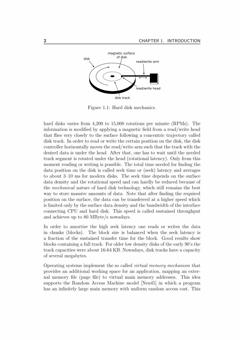
Figure 1.1: Hard disk mechanics.
hard disks varies from 4,200 to 15,000 rotations per minute (RPMs). Theinformation is modified by applying a magnetic field from a read/write headthat flies very closely to the surface following a concentric trajectory calleddisk track. In order to read or write the certain position on the disk, the diskcontroller horizontally moves the read/write arm such that the track with thedesired data is under the head. After that, one has to wait until the neededtrack segment is rotated under the head (rotational latency). Only from thismoment reading or writing is possible. The total time needed for finding thedata position on the disk is called seek time or (seek) latency and averagesto about 3–10 ms for modern disks. The seek time depends on the surfacedata density and the rotational speed and can hardly be reduced because ofthe mechanical nature of hard disk technology, which still remains the bestway to store massive amounts of data. Note that after finding the requiredposition on the surface, the data can be transferred at a higher speed whichis limited only by the surface data density and the bandwidth of the interfaceconnecting CPU and hard disk. This speed is called sustained throughputand achieves up to 80 MByte/s nowadays.
In order to amortize the high seek latency one reads or writes the datain chunks (blocks). The block size is balanced when the seek latency isa fraction of the sustained transfer time for the block. Good results showblocks containing a full track. For older low density disks of the early 90’s thetrack capacities were about 16-64 KB. Nowadays, disk tracks have a capacityof several megabytes.
Operating systems implement the so called virtual memory mechanism thatprovides an additional working space for an application, mapping an exter-nal memory file (page file) to virtual main memory addresses. This ideasupports the Random Access Machine model [Neu45] in which a programhas an infinitely large main memory with uniform random access cost. This
1.1. I/O-EFFICIENT ALGORITHMS AND MODELS 3
model has served as the most important basis of computer architecture andprogramming language development.
Since the memory view is unified in operating systems supporting virtualmemory, the application does not know where its working space and programcode are located: in the main memory or (partially) swapped out to the pagefile. This kind of abstraction does not have large running time penalties forapplications with a simple sequential data access pattern. The operatingsystem is even able to predict scanning patterns and to load the data inahead. For more complicated patterns these remedies are not useful and evencounterproductive: the swap file is accessed very frequently; the data codecan be swapped out in favor of data blocks; the swap file is highly fragmentedand thus many random input/output operations (I/Os) are needed even forscanning.
1.1 I/O-Efficient Algorithms and Models
The operating system cannot adapt to complicated access patterns of appli-cations dealing with massive data sets. Therefore, there is a need of explicithandling of external memory accesses. The applications and their underly-ing algorithms and data structures should care about the pattern and thenumber of external memory accesses (I/Os) which they cause.
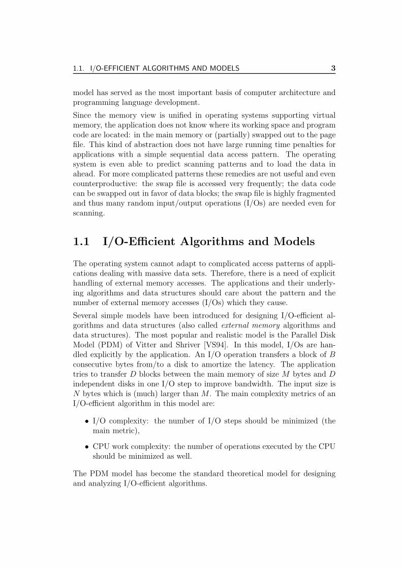
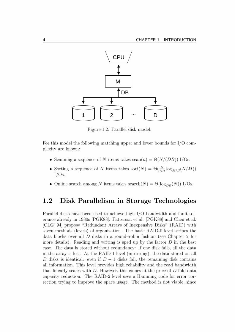
Several simple models have been introduced for designing I/O-efficient al-gorithms and data structures (also called external memory algorithms anddata structures). The most popular and realistic model is the Parallel DiskModel (PDM) of Vitter and Shriver [VS94]. In this model, I/Os are han-dled explicitly by the application. An I/O operation transfers a block of Bconsecutive bytes from/to a disk to amortize the latency. The applicationtries to transfer D blocks between the main memory of size M bytes and Dindependent disks in one I/O step to improve bandwidth. The input size isN bytes which is (much) larger than M . The main complexity metrics of anI/O-efficient algorithm in this model are:
• I/O complexity: the number of I/O steps should be minimized (themain metric),
• CPU work complexity: the number of operations executed by the CPUshould be minimized as well.
The PDM model has become the standard theoretical model for designingand analyzing I/O-efficient algorithms.
4 CHAPTER 1. INTRODUCTION
1 ...
CPU
M
2 D
DB
Figure 1.2: Parallel disk model.
For this model the following matching upper and lower bounds for I/O com-plexity are known:
• Scanning a sequence of N items takes scan(n) = Θ(N/(DB)) I/Os.
• Sorting a sequence of N items takes sort(N) = Θ( NDB
logM/B(N/M))I/Os.
• Online search among N items takes search(N) = Θ(logDB(N)) I/Os.
1.2 Disk Parallelism in Storage Technologies
Parallel disks have been used to achieve high I/O bandwidth and fault tol-erance already in 1980s [PGK88]. Patterson et al. [PGK88] and Chen et al.[CLG+94] propose “Redundant Arrays of Inexpensive Disks” (RAID) withseven methods (levels) of organization. The basic RAID-0 level stripes thedata blocks over all D disks in a round–robin fashion (see Chapter 2 formore details). Reading and writing is sped up by the factor D in the bestcase. The data is stored without redundancy: If one disk fails, all the datain the array is lost. At the RAID-1 level (mirroring), the data stored on allD disks is identical: even if D − 1 disks fail, the remaining disk containsall information. This level provides high reliability and the read bandwidththat linearly scales with D. However, this comes at the price of D-fold datacapacity reduction. The RAID-2 level uses a Hamming code for error cor-rection trying to improve the space usage. The method is not viable, since

1.2. DISK PARALLELISM IN STORAGE TECHNOLOGIES 5
for a modern computer environment it requires 39 hard disks to be realized.The RAID levels 3–6 are more practical and require only a small amount ofparity information to guarantee a high fault tolerance. They differ in howand where the parity data is stored. The best (parallel) performance havethe levels 5 and 6 because they distribute the parity data blocks across all Ddisks, such that there is no bottleneck.
All RAID levels can be realized in software in the framework of the Par-allel Disk Model (see for instance the software RAID in Linux). Since theRAID disk parallelism can (partially) mitigate the I/O-bottleneck problemand is very easy to use (a RAID array looks like a single disk for the user),the RAID solutions became standard and are implemented in many hard-ware disk controllers to off-load the CPU. In addition to the standard levels,the (hardware) implementations offer nested RAID levels that combine theproperties of several levels: A RAID-50 (RAID-5+0) is a RAID-0 stripedacross superdisks realized as RAID-5 arrays. Other popular combinationsare: RAID-01, RAID-10, RAID-30 and RAID-100.
A network-attached storage (NAS) is a data storage technology that canbe connected to a computer network to provide centralized data storage forclients [MT03]. NAS can be realized as a dedicated server running a minimal-functionality operating system with support of a file-based protocol like NFSor CIFS to export the data to the clients. NAS has several advantagesover the direct attached storage (e. g. local hard disks). Since NAS serversexecute only file-serving functions, they are more reliable (going down lessfrequently) and faster, if the network bandwidth is high. To exploit diskparallelism, NAS servers can use local RAID arrays to store the data.
A storage area network (SAN) is a network designed to attach storage el-ements (e. g. hard disks, RAID controllers, tapes) to servers [MT03]. Incontrast to NAS, the protocols used in a SAN are block-oriented, similar tothe protocols used in hardware interfaces like ATA and SCSI. A SAN consistsof a communication infrastructure, which provides physical connections, anda management layer, which organizes the connections, storage elements, andcomputer systems so that data transfer is secure and robust. The data storedin SANs can be striped across hundreds of disks to provide high bandwidth toaccess to the same files. SAN technology has excellent performance, however,the cost of the SAN equipment (disks, network) is relatively high.
The goal of distributed and parallel file systems (e. g. AFS [HKM+88],Google FS [GGL03], xFS [ADN+96], Swift [CL91], GPFS [SH02], see also ref-erences in [MSS03, Chapter 13] and [GGL03]) is to provide high-performanceand reliable storage of user files. The file data is split into chunks and a num-
6 CHAPTER 1. INTRODUCTION
1
CPU
...
M
2 D
DB
L2
B
B
CPU
L1
R1
R2
R3 ...
2
1
3
Figure 1.3: Memory hierarchy.
ber of chunk replicas are stored at several computers (storage nodes). Thisallows to achieve a high fault tolerance: If a disk at the node or the node it-self is broken, then the remaining chunk replicas are copied to another nodesto restore the data redundancy. The I/O bandwidth and response time canbe improved as well: The chunks of the requested file can be read in parallelfrom several nodes and the closest replica is requested from the availableones.
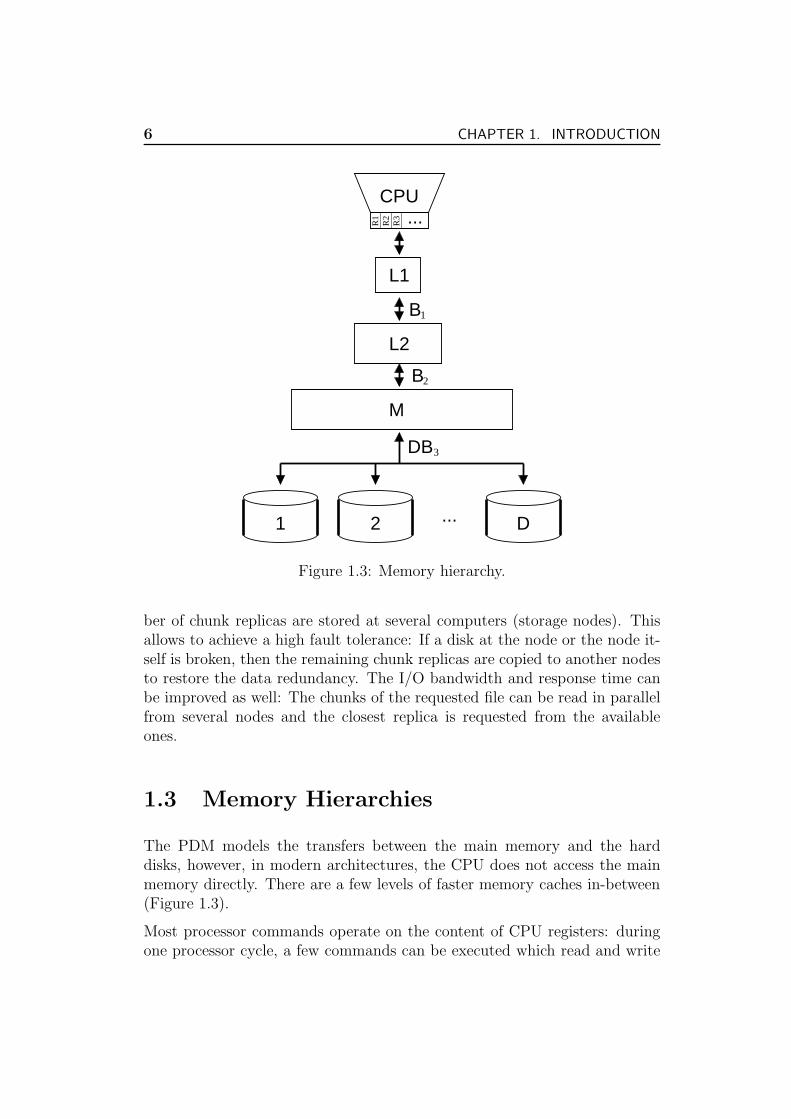
1.3 Memory Hierarchies
The PDM models the transfers between the main memory and the harddisks, however, in modern architectures, the CPU does not access the mainmemory directly. There are a few levels of faster memory caches in-between(Figure 1.3).
Most processor commands operate on the content of CPU registers: duringone processor cycle, a few commands can be executed which read and write
1.3. MEMORY HIERARCHIES 7
the registers in parallel. When the data is to be loaded from the mainmemory into the registers, the level one the (L1) cache is checked first to seewhether it already contains the content of the needed memory cell (cachehit). Otherwise it must be loaded from the next cache level (cache miss).If a register value is to be stored in memory, it is buffered in the L1 cache.This value will be flushed only if the cache is full and a place for new datais needed. The L1 cache is a small (a few KBytes) and fast memory whichallows up to two (or few) accesses per CPU cycle. If the data is not cachedin L1, the larger (up to several MBytes with the current technology) leveltwo (L2) cache is accessed. The access time of the L2 cache is about 10cycles. The transfers between the L1 and L2 caches use block sizes about 16-32 bytes. Both L1 and L2 caches lie on the same chip as the main processor.Some modern processors also have off-the-chip L3 caches, however, they arerather expensive. The transfer block of the main memory and the L2/L3cache is 128-256 Bytes (i.e. for the Pentium 4).
The main memory is cheaper and slower than the caches. Cheap dynamicrandom access memory, used in the majority of computer systems, has anaccess latency up to 60 ns. However, for a blocked access a high bandwidthof several GByte/s can be achieved.
The translation lookaside buffer (TLB) is another caching mechanism in pro-cessors. TLBs cache some parts of large tables which store the logical tophysical address region mappings. The caching speeds up the virtual memorymechanism of operating systems. TLB misses might be the main bottleneckfor algorithms: a TLB miss could be quite expensive (up to 100 CPU cycles);the cache itself is small (32-128 entries) 3.
The memory hierarchy in computer systems is a natural phenomenon: a fasthuge memory with uniform memory access cannot exist because the accesstime is correlated with the speed of light. Therefore the faster memories(caches) are placed closer to the processor. Another reason is cost efficiency:Prices for a byte for L1 caches and hard disks differ in many orders of mag-nitude. One can only afford to keep a small, most frequently used fractionof the data in fast memory. The number of memory hierarchy levels havingdifferent access latencies and speed is growing: in 1986, Intel’s 386 processorhad a single off-chip cache, nowadays the IBM Power 5 series already has a144 MByte L3 cache off-chip shared among several processors.
The discrepancy between the speed of CPUs and the latency of the lowerhierarchy levels grows very quickly: the speed of processors is improved by
3The Calibrator tool http://monetdb.cwi.nl/Calibrator/ reports a TLB miss-latency of 54 CPU cycles on our 3.0 GHz Pentium 4 processor with only 32 TLB entries.
8 CHAPTER 1. INTRODUCTION
about 55 % yearly, the hard disk access latency only by 9 % [Pat04]. There-fore, the algorithms which are aware of the memory hierarchy will continue tobenefit in the future and the development of such algorithms is an importanttrend in computer science.
The PDM model only describes a single level in the hierarchy. An algo-rithm tuned to make a minimum number of I/Os between two particularlevels could be I/O-inefficient on other levels. The cache-oblivious modelin [FLPR99] avoids this problem by not providing the knowledge of theblock size B and main memory size M to the algorithm. The benefit ofsuch an algorithm is that it will be I/O-efficient on all levels of the memoryhierarchy across many systems without fine tuning for any particular realmachine parameters. Many basic algorithms and data structures have beendesigned for this model: sorting [FLPR99], matrix transposition and multipli-cation [FLPR99], priority queues [ABD+02], dictionaries [BDIW02], breadth-first-search [ABD+02, BFMZ04], depth-first-search [ABD+02], shortest paths[BFMZ04], minimum spanning trees [ABD+02], . . .. A drawback of cache-oblivious algorithms playing a role in practice is that they are only asymp-totically I/O-optimal. The constants hidden in the O() notation of theirI/O-complexity are significantly larger than the constants of the correspond-ing I/O-efficient PDM algorithms (on a particular memory hierarchy level).For instance, a tuned cache-oblivious funnel sort implementation [Chr05] is2.6–4.0 times slower than our I/O-efficient sorter from Stxxl (Section 3.5)for out-of-memory inputs [Osi06, AMO07]. A similar funnel sort implemen-tation is up to two times slower than the I/O-efficient sorter from TPIElibrary (Section 1.9) for large inputs [BFV04]. The reason for this is thatthese I/O-efficient sorters are highly optimized to minimize the number oftransfers between the main memory and the hard disks where the imbalancein the access latency is the largest (up to 106 times). Cache-oblivious imple-mentations lose on the inputs, exceeding the main memory size, because (upto a constant factor) they do more I/Os at the last level of memory hierarchy.
In this thesis we concentrate on extremely large out-of-memory inputs, there-fore we will design and implement algorithms and data structures efficient inthe PDM.

1.4. ALGORITHM ENGINEERING FOR LARGE DATA SETS 9
1.4 Algorithm Engineering for Large Data
Sets
Theoretically, I/O-efficient algorithms and data structures have been devel-oped for many problem domains: graph algorithms, string processing, com-putational geometry, etc. (see the surveys [MSS03, Vit01]). Some of themhave been implemented: sorting, matrix multiplication [VV96], search trees[Chi95, PAAV, AHVV99, AAG03], priority queues [BCFM00], text process-ing [CF02]. However only few of the existing I/O-efficient algorithms havebeen studied experimentally. As new algorithmic results rely on previousones, researchers, which would like to engineer practical implementations oftheir ideas and show the feasibility of external memory computation for thesolved problem, need to invest much time in the careful design of unimple-mented underlying external algorithms and data structures. Additionally,since I/O-efficient algorithms deal with hard disks, a good knowledge of low-level operating system issues is required when implementing details of I/Oaccesses and file system management. This delays the transfer of theoreticalresults into practical applications, which will have a tangible impact for in-dustry. Therefore one of the primary goals of algorithm engineering for largedata sets is to create software frameworks and libraries which handle boththe low-level I/O details efficiently and in an abstract way, and provide well-engineered and robust implementations of basic external memory algorithmsand data structures.
1.5 C++ Standard Template Library
The Standard Template Library (STL) [SL94] is a C++ library which is in-cluded in every C++ compiler distribution. It provides basic data structures(called containers) and algorithms.
STL containers are generic and can store any built-in or user data typethat supports some elementary operations (e.g. copying and assignment).STL algorithms are not bound to a particular container: an algorithm canbe applied to any container that supports the operations required for thisalgorithm (e.g. random access to its elements). This flexibility significantlyreduces the complexity of the library.
STL is based on the C++ template mechanism. The flexibility is supportedusing compile-time polymorphism rather than the object oriented run-timepolymorphism. The run-time polymorphism is implemented in languages
10 CHAPTER 1. INTRODUCTION
like C++ with the help of virtual functions that usually cannot be inlined byC++ compilers. This results in a high per-element penalty of calling a vir-tual function. In contrast, modern C++ compilers minimize the abstractionpenalty of STL being able to inline many functions.
STL containers include: std::vector (an unbounded array),std::list, std::priority queue, std::stack, std::deque, std::set,std::multiset (allows duplicate elements), std::map (allows mappingfrom one data item (a key) to another (a value)), std::multimap (allows du-plicate keys), . . .. Containers based on hashing (hash set, hash multiset,hash map and hash multimap) are not yet standardized and distributed asan STL extension.
Iterators are an important part of the STL library. An iterator is a kindof handle used to access items stored in data structures. Iterators allowto perform the following operations: read/write the value pointed by theiterator, move to the next/previous element in the container, move by somenumber of elements forward/backward (random access).
STL provides a large number of algorithms performing scanning, searchingand sorting. The implementations accept iterators that posses a certainset of operations described above. Thus, the STL algorithms will work onany container with iterators obeying to required capabilities. To achieveflexibility, STL algorithms are parameterized with objects, overloading thefunction operator (operator()). Such objects are called functors. A functorcan, for instance, define the sorting order for the STL sorting algorithm orkeep the state information in functions passed to other functions. Since thetype of the functor is a template parameter of an STL algorithm, the functionoperator does not need to be virtual and can easily be inlined by the compiler,thus avoiding the function call costs.
The STL library is well accepted, its generic approach and principles arefollowed in other famous C++ libraries like Boost [Kar05] and CGAL[FGK+00].
1.6 The Goals of Stxxl
Several external memory software library projects (LEDA-SM [CM99] andTPIE [ABH+03]) were started to reduce the gap between theory and practicein external memory computing. They offer frameworks which aim to speedup the process of implementing I/O-efficient algorithms, abstracting away
1.7. SOFTWARE FACTS 11
the details of how I/O is performed. See Section 1.9 for an overview of theselibraries.
The TPIE and LEDA-SM projects are excellent proofs of the concepts of theexternal memory paradigm, but they miss some practice-relevant featureswhich are important for applications. This led us to start the developmentof a performance–oriented library of external memory algorithms and datastructures, namely Stxxl, which tries to avoid those obstacles. The Stxxl
library is the main contribution of this thesis.
The following here are some key features of Stxxl:
• Transparent support of parallel disks. The library provides implemen-tations of basic parallel disk algorithms. Stxxl is the only externalmemory algorithm library supporting parallel disks. Such a feature wasannounced for TPIE in [Ven94, ABH+03].
• The library is able to handle problems of a very large size (up to dozensof terabytes).
• Improved utilization of computer resources. Stxxl explicitly supportsoverlapping between I/O and computation. Stxxl implementationsof external memory algorithms and data structures benefit from theoverlapping of I/O and computation.
• Small constant factors in I/O volume. A unique library feature “pipelin-ing” can save more than half the number of I/Os performed by manyalgorithms.
• Shorter development times due to well known STL-compatible inter-faces for external memory algorithms and data structures. STL al-gorithms can be directly applied to Stxxl containers (code reuse);moreover, the I/O complexity of the algorithms remains optimal inmost cases.
1.7 Software Facts
Stxxl is distributed under the Boost Software License4 which isan open source license allowing free commercial use. The sourcecode, installation instructions and documentations are available under
4http://www.boost.org/more/license_info.html
12 CHAPTER 1. INTRODUCTION
http://stxxl.sourceforge.net/. According to the well known SLOC-Count 5 tool of David A. Wheeler, the release branch of the Stxxl projectnot including applications has about 25,000 physical source lines of code(SLOC).
1.8 Stxxl Users
Here is a list of active Stxxl users we know about:
• University of Karlsruhe, Germany (text processing, graph algorithms,practical courses)
• Max-Planck-Institut fur Informatik, Germany (graph algorithms)
• University of Rome “La Sapienza”, Italy (connected components)
• University of Texas at Austin, USA (gaussian elimination)
• Bitplane AG, Switzerland (visualization and analysis of 3D and 4Dmicroscopic images)
• Philips Research, The Netherlands (differential cryptographic analysis)
• Dalhousie University, Canada (N -gram extraction)
• Florida State University, USA (construction of Voronoi diagrams)
• Montefiore Institute, Belgium (big sparse matrices)
• University of British Columbia, Canada (topology analysis of large net-works)
• Bayes Forecast, Spain (statistics and time series analysis)
• Indian Institute of Science in Bangalore, India (suffix array construc-tion)
• Rensselaer Polytechnic University, USA (suffix array construction)
• Institut francais du perole, France (analysis of seismic files)
• Northumbria University, UK (search trees)
5http://www.dwheeler.com/sloccount/

1.9. RELATED WORK 13
• University of Trento, Italy (text compression)
• Norwegian University of Science and Technology in Trondheim, Norway(suffix array construction)
1.9 Related Work
TPIE [Ven94, APV02] was the first large software project implementing I/O-efficient algorithms and data structures. The library provides implementa-tions of I/O efficient sorting, merging, matrix operations, many (geometric)search data structures (B+-tree, persistent B+-tree, R-tree, K-D-B-tree, KD-tree, Bkd-tree) and the logarithmic method. The work on the TPIE projectis in progress.
LEDA-SM [CM99] external memory library was designed as an extensionto the LEDA library [MN99] for handling large data sets. The library of-fers implementations of I/O-efficient sorting, external memory stack, queue,radix heap, array heap, buffer tree, array, B+-tree, string, suffix array, ma-trices, static graph, and some simple graph algorithms. However, the datastructures and algorithms cannot handle more than 231 elements. The de-velopment of LEDA-SM has been stopped. LEDA releases later than theversion 4.2 are not supported by the last LEDA-SM version 1.3. The latestcompiler, LEDA-SM 1.3 can be compiled with, is the g++ version 2.95.
LEDA-SM and TPIE libraries currently only offer single disk external mem-ory algorithms and data structures. They are not designed to explicitly sup-port an overlapping between I/O and computation. The overlapping largelyrelies on the operating system that caches and prefetches data according to ageneral purpose policy, which cannot be as efficient as the explicit approach.Furthermore, on most of the operating systems, the overlapping based on thesystem cache requires additional copies of the data, which leads to compu-tational and internal memory overhead.
The list of algorithms and data structures available in TPIE, LEDA-SM andStxxl libraries is shown in Table 1.1.
Database engines use I/O-efficient search trees and sorting to execute SQLqueries, evaluating huge sets of table records. The idea of pipelined executionof the algorithms which process large data sets not fitting into the mainmemory is well known in relational database management systems [SKS01].The pipelined execution strategy allows to execute a database query witha minimum number of external memory accesses, to save memory space tostore intermediate results, and to obtain the first result as soon as possible.

14 CHAPTER 1. INTRODUCTION
Table 1.1: Algorithms and data structures of the external memory libraries.
Function TPIE LEDA-SM Stxxl
sorting√ √ √
stack√ √ √
queue√ √ √
deque — —√
array/vector —√ √
matrix operations√ √
—suffix array —
√ √(extension)
search trees B+-tree, K-D-B-tree B+-tree B+-treepersist. B+-tree buffer treeR-tree, KD-tree
Bkd-treepriority queue — array heap sequence heap
radix heappipelined algorithms — —
√
The design framework FG [DC05] is a programming environment for parallelprograms running on clusters. In this framework, parallel programs are splitinto series of asynchronous stages which are executed in the pipelined fashionwith the help of multithreading. The pipelined execution allows to mitigatedisk latency of external data accesses and communication network latencyof remote data accesses. I/O and communication could be automaticallyoverlapped with computation stages by the scheduler of FG environment.
Berkeley DB [OBS00] is recognized as the best open source external memoryB+-tree implementation. It has a dual license and is not free for industry.Berkeley DB has very large user base, among those are amazon.com, Googleand Motorola. Many free open source programs use Berkeley DB as theirdata storage backend (e.g. MySQL data base system).
There are several libraries for advanced models of computation which fol-low the interface of STL. The Standard Template Adaptive Parallel Library(STAPL) is a parallel library designed as a superset of the STL. It is sequen-tially consistent for functions with the same name and performs on uni- ormulti-processor systems that utilize shared or distributed memory [AJR+01].
MCSTL (Multi-Core Standard Template Library) project [Sin06] has beenstarted in 2006 at the University of Karlsruhe. The library is an implemen-tation of the STL which uses multiple processors and multiple cores of a
1.10. OUTLINE 15
processor with shared memory. It already has implementations of parallelsorting, merging, random permutation, searching, scanning. MCSTL is cur-rently being used to parallelize the internal work of Stxxl external memorysorting.
There is a number of libraries which provide persistent containers [Unia,Unib, GND99, Nel98, Kni, SKW92]. Persistent STL-compatible containersare implemented in [Ste98, Gsc01]. These containers can keep (some of)the elements in external memory transparently to the user. In contrast toStxxl, these libraries do not guarantee the I/O-efficiency of the containers,e. g. the PSTL [Gsc01] library implements search trees as I/O-inefficientred-black trees.
The content of this thesis is partially based on our contributions which havebeen already published in a number of refereed conference and journal pa-pers. The design rational of Stxxl has been investigated in [DKS05a]. Theextended version of this paper has appeared as a technical report [DKS05b].The results on engineering algorithms for large graphs have been published in[DSSS04] (minimum spanning forests) and in [ADM06] (breadth first search).I/O-efficient algorithms for construction of suffix arrays are the subject of thepaper [DMKS05]. An extended version will appear as a journal publication[DKMS06].
1.10 Outline
This thesis is organized as follows.
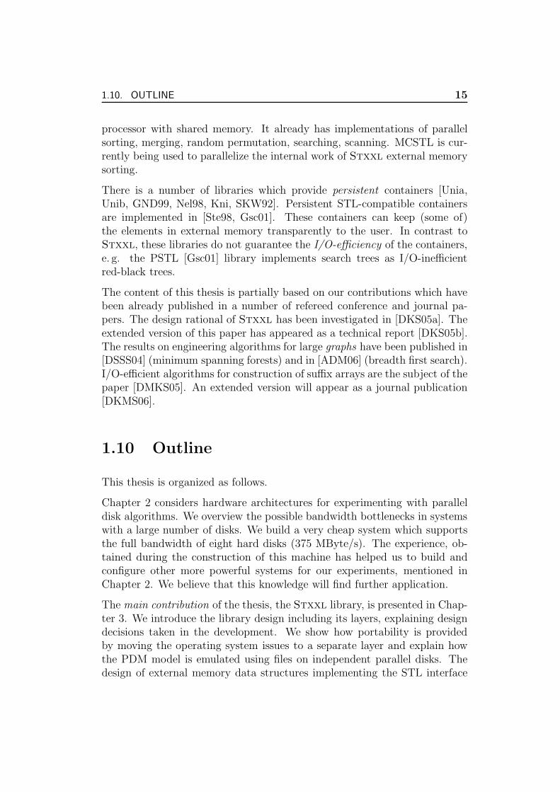
Chapter 2 considers hardware architectures for experimenting with paralleldisk algorithms. We overview the possible bandwidth bottlenecks in systemswith a large number of disks. We build a very cheap system which supportsthe full bandwidth of eight hard disks (375 MByte/s). The experience, ob-tained during the construction of this machine has helped us to build andconfigure other more powerful systems for our experiments, mentioned inChapter 2. We believe that this knowledge will find further application.
The main contribution of the thesis, the Stxxl library, is presented in Chap-ter 3. We introduce the library design including its layers, explaining designdecisions taken in the development. We show how portability is providedby moving the operating system issues to a separate layer and explain howthe PDM model is emulated using files on independent parallel disks. Thedesign of external memory data structures implementing the STL interface

16 CHAPTER 1. INTRODUCTION
is discussed. We compare the performance of our containers with the perfor-mance of data structures of LEDA-SM, TPIE and Berkeley DB using variousbenchmarks. Examples of the compatibility and combined usage of STL al-gorithms and Stxxl containers will be demonstrated. In Section 3.5, weengineer a parallel disk sorting that has almost perfect overlap of I/O andcomputation and has an I/O cost approaching the lower bound. Previousalgorithms have either a suboptimal I/O volume or cannot guarantee thatI/O and computation can always be overlapped. We compare its perfor-mance with the performance of LEDA-SM and TPIE sorters. Furthermore,we introduce the idea of external algorithm pipelining in the context of anexternal memory software library and show how pipelining is implementedin the Stxxl Streaming layer via objects with an iterator-like interface. Asmall example demonstrates the I/O savings gained by the use of pipelining.
Stxxl has been successfully applied in implementation projects that studiedvarious I/O-efficient algorithms from the practical point of view (Chapters 4and 5). The fast algorithmic components of the Stxxl library gave theimplementations an opportunity to solve problems of very large sizes on alow-cost hardware in record time.
The chapter starts with a small benchmark (maximal independent set com-putation), which we implement using TPIE, LEDA-SM and Stxxl. We runthese implementations to compare the performance of some components ofthe library on a real graph application.
Furthermore, we investigate the feasibility of minimal spanning forest com-putation in external memory. Due to the Stxxl, our external memory MSFimplementation is only 2–5 times slower than a good internal algorithm withsufficient memory space. We modify the minimum spanning forest algorithmto derive a fast I/O-efficient algorithm for computing connected componentsand/or spanning forests.
The next study, investigating the feasibility of external memory breadth-first search (BFS), is surveyed in Section 4.5. The study compares twoimplementations of the external memory BFS algorithms [MR99, MM02].The implementations heavily use Stxxl pipelining and can compute BFSdecompositions for very large real and synthetic graphs within hours on amodest PC.
In Section 4.6 we design a practical algorithm that lists and counts all tri-angles in huge graphs. The triangle information is used to analyze the prop-erties of (social) networks, like “clusterness” and transitivity. With the helpof Stxxl we find all triangles of a huge web crawl graph in a few hours.
The last graph application we have designed in this thesis is coloring (Sec-
1.10. OUTLINE 17
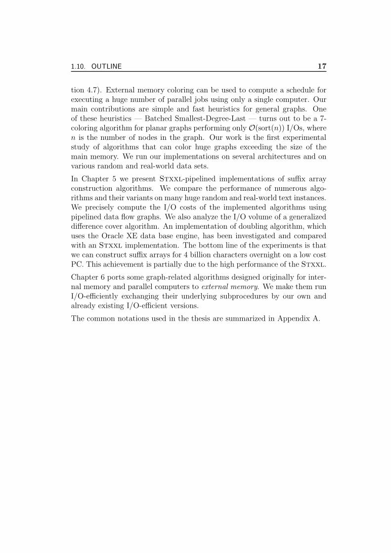
tion 4.7). External memory coloring can be used to compute a schedule forexecuting a huge number of parallel jobs using only a single computer. Ourmain contributions are simple and fast heuristics for general graphs. Oneof these heuristics — Batched Smallest-Degree-Last — turns out to be a 7-coloring algorithm for planar graphs performing only O(sort(n)) I/Os, wheren is the number of nodes in the graph. Our work is the first experimentalstudy of algorithms that can color huge graphs exceeding the size of themain memory. We run our implementations on several architectures and onvarious random and real-world data sets.
In Chapter 5 we present Stxxl-pipelined implementations of suffix arrayconstruction algorithms. We compare the performance of numerous algo-rithms and their variants on many huge random and real-world text instances.We precisely compute the I/O costs of the implemented algorithms usingpipelined data flow graphs. We also analyze the I/O volume of a generalizeddifference cover algorithm. An implementation of doubling algorithm, whichuses the Oracle XE data base engine, has been investigated and comparedwith an Stxxl implementation. The bottom line of the experiments is thatwe can construct suffix arrays for 4 billion characters overnight on a low costPC. This achievement is partially due to the high performance of the Stxxl.
Chapter 6 ports some graph-related algorithms designed originally for inter-nal memory and parallel computers to external memory. We make them runI/O-efficiently exchanging their underlying subprocedures by our own andalready existing I/O-efficient versions.
The common notations used in the thesis are summarized in Appendix A.
18 CHAPTER 1. INTRODUCTION

Chapter 2
Building Experimental ParallelDisk Systems
Experiments with single disk external memory algorithms do not requirea special hardware to be run on. All off-the-shelf desktop computers areequipped with at least one hard disk which stores an operating system andkeeps the working space of applications. Such systems are readily fit forexperimenting with I/O-efficient algorithms designed for a single disk.
The I/O bandwidth of a modern hard disk is limited to 70–80 MB/s, thebandwidth of transfers between memory and CPU is much higher: severalgigabytes per second. The relatively low disk bandwidth can be the bottle-neck of an external memory algorithm. This bottleneck can be mitigated oreven eliminated when by using a RAID.
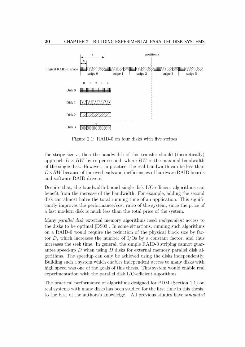
The RAID (redundant array of independent disks; originally redundant arrayof inexpensive disks) array level 0 (RAID-0 for short) is a way of storing datadistributed over multiple disks [CLG+94]. Usually, all disks of a RAID areidentical. A RAID acts as a single logical disk to the operating system.RAID-0 employs the technique of striping, which involves partitioning eachdrive’s storage space into units of size c bytes (usually a power of two, rangingfrom 4 KBytes to 128 KBytes). Each chunk of size s = D × c of the RAIDlogical space is called stripe, where D is the number of disks in the RAID.Stripes are mapped in an interleaved fashion to the disks: logical RAID diskposition x is mapped to position c⌊x
s⌋ + (x mod c) on disk ⌊x mod s
c⌋ (see
Figure 2.1). This mapping can be performed by a special device controller,called RAID-controller, or via software by the RAID emulation driver (e.g.the Linux software RAID driver). If an application reads a block from RAID-0 or writes a block to RAID-0 and the size of the block is a (big) multiple of
19
20 CHAPTER 2. BUILDING EXPERIMENTAL PARALLEL DISK SYSTEMS
s
c
Logical RAID−0 space
Disk 0
Disk 1
Disk 2
Disk 3
position x
43210
stripe 0 stripe 1 stripe 2 stripe 3 stripe 5
Figure 2.1: RAID-0 on four disks with five stripes
the stripe size s, then the bandwidth of this transfer should (theoretically)approach D × BW bytes per second, where BW is the maximal bandwidthof the single disk. However, in practice, the real bandwidth can be less thanD×BW because of the overheads and inefficiencies of hardware RAID boardsand software RAID drivers.
Despite that, the bandwidth-bound single disk I/O-efficient algorithms canbenefit from the increase of the bandwidth. For example, adding the seconddisk can almost halve the total running time of an application. This signifi-cantly improves the performance/cost ratio of the system, since the price ofa fast modern disk is much less than the total price of the system.
Many parallel disk external memory algorithms need independent access tothe disks to be optimal [DS03]. In some situations, running such algorithmson a RAID-0 would require the reduction of the physical block size by fac-tor D, which increases the number of I/Os by a constant factor, and thusincreases the seek time. In general, the simple RAID-0 striping cannot guar-antee speed-up D when using D disks for external memory parallel disk al-gorithms. The speedup can only be achieved using the disks independently.Building such a system which enables independent access to many disks withhigh speed was one of the goals of this thesis. This system would enable realexperimentation with the parallel disk I/O-efficient algorithms.
The practical performance of algorithms designed for PDM (Section 1.1) onreal systems with many disks has been studied for the first time in this thesis,to the best of the authors’s knowledge. All previous studies have simulated
2.1. HARDWARE DISK INTERFACES 21
the parallel disks in software.
2.1 Hardware Disk Interfaces
Currently, there are two types of hardware interfaces which connect harddisks with computers: IDE (Integrated Drive Electronics) and SCSI (SmallComputer Systems Interface). Several versions of the IDE interface werestandardized under the name ATA (Advanced Technology Attachment). Theoriginal ATA hard disks use 40 or 80 wire cables (parallel ATA). A newerversion of the ATA standard enables transferring the information over a cablewith the same speed or faster using only a few wires (serial ATA = SATA).The parallel ATA (PATA) permits to assign two disks to the same channel,which can result in less than expected parallel disk performance, even if theATA bus rate is higher than the total maximum bandwidth of the two disks.The reason is that the original IDE/ATA interface protocol was not designedfor concurrent access to the disks, the disks “must take turns”. A parallelATA channel permits transfer rates up to 133 MByte/s.
Serial ATA has some crucial differences to parallel ATA that improve perfor-mance. Since the cost of an additional channel controller on a circuit is small,and a little space is required for cables and cable headers, SATA specifies onlya single device per channel to be used. Another feature is the hardware sup-port of disk request queuing (native command queuing): A hard disk canreceive more than one I/O request at a time and decide on its own in whichorder the requests will be served. This allows a lot of optimizations, pro-vided the knowledge about the seek times and rotational position. A SATAchannel can sustain a bandwidth up to 150 or 300 MByte/s depending onthe used standard.
Low-cost or middle range PCs have an on-board controller with at leasttwo ATA or four SATA channels. They can theoretically support two/fourdisks at full speed (the maximum sustained transfer rate of modern disks is60–80 MB/s). The logic of an IDE controller is kept simple to reduce theprice of hardware, therefore many low level details of the ATA protocol areimplemented in software and executed by the main CPU.
SCSI standard has been initially developed to support many disks which canbe accessed concurrently at high speed. One Ultra320 SCSI (U320) channelcan connect up to 15 disks and has a bandwidth of 320 MB/s. The SCSI buscontroller is capable of controlling the hard disk drives without any work bythe CPU. Native support of command queuing already existed in very early
22 CHAPTER 2. BUILDING EXPERIMENTAL PARALLEL DISK SYSTEMS
versions of the SCSI standard. Also, all drives on a SCSI channel are ableto operate at the same time due to the advanced protocol logic, implementedin hardware. Therefore one U320 channel can support up to four moderndisks at almost full speed (60–80 MByte/s).
The SCSI interface has apparent advantages over IDE/ATA one, however,the price of SCSI hardware (controllers and hard disk drives) is 3–8 timeshigher than the price of comparable IDE/ATA equipment. We have tried tofind out whether it is possible to build an affordable high performance multidisk system using IDE/ATA technology.
2.2 Busses, Controllers, Chipsets
As above mentioned, an ordinary PC can already support four hard disksconnected to the on-board PATA controller. However, in order to avoidbottlenecks and channel contention, it is better to have only one disk perIDE channel. Thus, only two ATA drives can be supported at full speed.
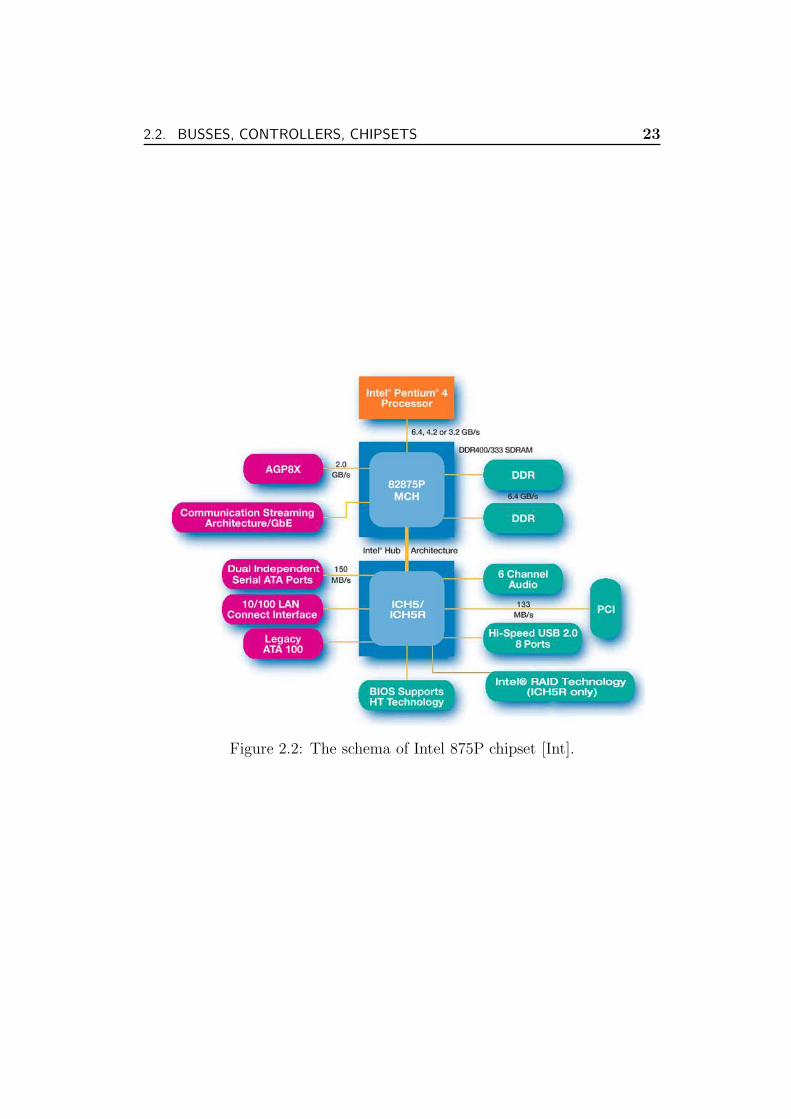
In order to support more disks one has to use more controllers, which areinstalled in a PCI bus slot of the PC. There are several variants of PCIbusses, the older version of the bus protocol can transfer 32 bits in a cycleand has a cycle frequency of 33 MHz, giving the maximum transfer rate of133 MByte/s. Theoretically, this would be enough for only two disks with atransfer rate of 66 MByte/s (we take 66 MByte/s as the bandwidth of onedisk in calculations), but in practice, due to the bus control overhead, thesustained bandwidth could be less. Cheap desktop systems usually have onlyone 32bit/33MHz bus. The chipset schema of such a system is presented inFigure 2.2. This system can support four (S)ATA disks at most at full speed:two disks connect to the onboard Serial ATA controller, the other two requirea PCI bus (S)ATA controller. The Intel hub connection between the memorycontroller hub (MCH) and the I/O controller hub (ICH) chips is fast enoughto sustain the bandwidth of four disks.
Some chipsets/mainboards do include an additional hardware RAID con-troller with two (S)ATA channels. The Intel 875P chipset has such an option(see Figure 2.2). The RAID controller could be configured for independentaccess to the disks, i.e. RAID is switched off. This means that this cheapsystem can already support up to six (S)ATA disks without bottlenecks inthe busses.
Newer PCI standards allow larger bus widths of 64 bits and/or higher cyclefrequencies 66, 100 or 133 MHz. A 64bit/133MHz PCI controller can transfer
2.2. BUSSES, CONTROLLERS, CHIPSETS 23
Figure 2.2: The schema of Intel 875P chipset [Int].
24 CHAPTER 2. BUILDING EXPERIMENTAL PARALLEL DISK SYSTEMS
at a speed of 533 MB/s, this bandwidth is enough for eight hard disk driveswith a bandwidth of 66 MB/s. SATA controllers with many ports have beenreleased recently : The Promise SATAII150 SX8 has eight SATA ports, eachoperating at a speed up to 150 MB/s. The manufacturer reports more than500 MB/s sustained throughput for sequential access for the controller.
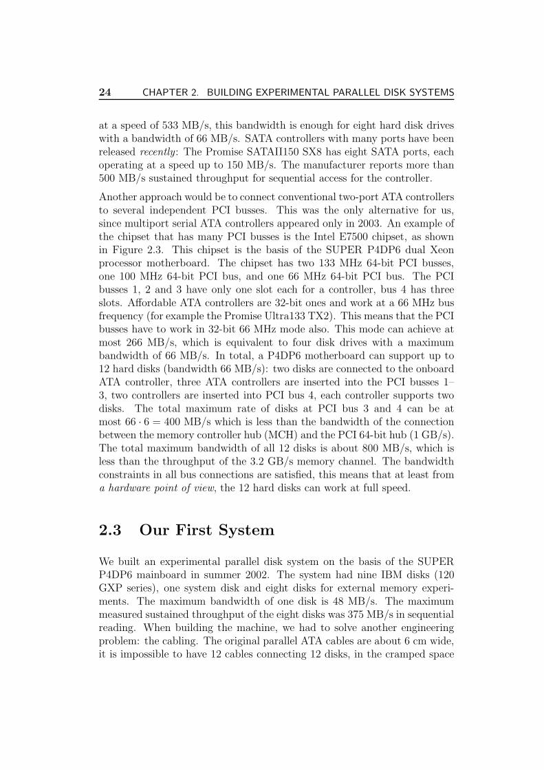
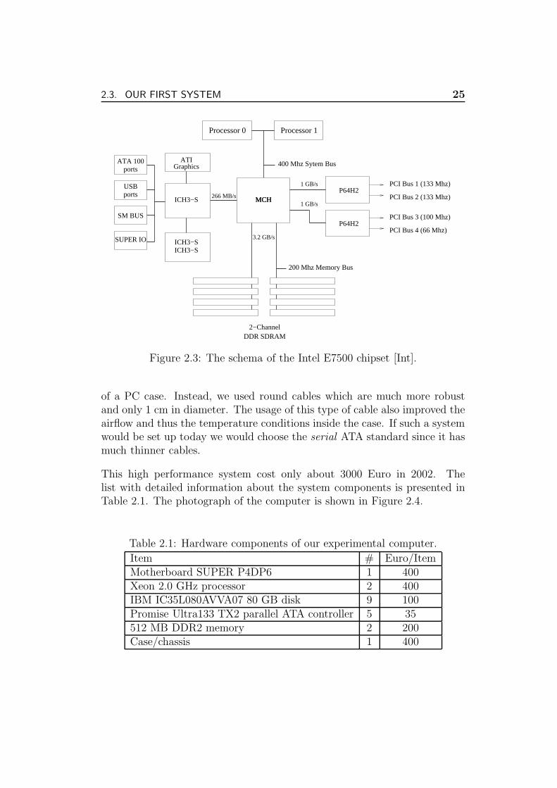
Another approach would be to connect conventional two-port ATA controllersto several independent PCI busses. This was the only alternative for us,since multiport serial ATA controllers appeared only in 2003. An example ofthe chipset that has many PCI busses is the Intel E7500 chipset, as shownin Figure 2.3. This chipset is the basis of the SUPER P4DP6 dual Xeonprocessor motherboard. The chipset has two 133 MHz 64-bit PCI busses,one 100 MHz 64-bit PCI bus, and one 66 MHz 64-bit PCI bus. The PCIbusses 1, 2 and 3 have only one slot each for a controller, bus 4 has threeslots. Affordable ATA controllers are 32-bit ones and work at a 66 MHz busfrequency (for example the Promise Ultra133 TX2). This means that the PCIbusses have to work in 32-bit 66 MHz mode also. This mode can achieve atmost 266 MB/s, which is equivalent to four disk drives with a maximumbandwidth of 66 MB/s. In total, a P4DP6 motherboard can support up to12 hard disks (bandwidth 66 MB/s): two disks are connected to the onboardATA controller, three ATA controllers are inserted into the PCI busses 1–3, two controllers are inserted into PCI bus 4, each controller supports twodisks. The total maximum rate of disks at PCI bus 3 and 4 can be atmost 66 · 6 = 400 MB/s which is less than the bandwidth of the connectionbetween the memory controller hub (MCH) and the PCI 64-bit hub (1 GB/s).The total maximum bandwidth of all 12 disks is about 800 MB/s, which isless than the throughput of the 3.2 GB/s memory channel. The bandwidthconstraints in all bus connections are satisfied, this means that at least froma hardware point of view, the 12 hard disks can work at full speed.
2.3 Our First System
We built an experimental parallel disk system on the basis of the SUPERP4DP6 mainboard in summer 2002. The system had nine IBM disks (120GXP series), one system disk and eight disks for external memory experi-ments. The maximum bandwidth of one disk is 48 MB/s. The maximummeasured sustained throughput of the eight disks was 375 MB/s in sequentialreading. When building the machine, we had to solve another engineeringproblem: the cabling. The original parallel ATA cables are about 6 cm wide,it is impossible to have 12 cables connecting 12 disks, in the cramped space
2.3. OUR FIRST SYSTEM 25
MCHMCHICH3−S
SM BUS
SUPER IO
ATA 100ports
USBports
ATI
ICH3−SICH3−S
Graphics
DDR SDRAM2−Channel
Processor 1Processor 0
P64H2PCI Bus 3 (100 Mhz)
PCI Bus 4 (66 Mhz)
200 Mhz Memory Bus
400 Mhz Sytem Bus
P64H2PCI Bus 2 (133 Mhz)
PCI Bus 1 (133 Mhz)1 GB/s
1 GB/s
3.2 GB/s
266 MB/s
Figure 2.3: The schema of the Intel E7500 chipset [Int].
of a PC case. Instead, we used round cables which are much more robustand only 1 cm in diameter. The usage of this type of cable also improved theairflow and thus the temperature conditions inside the case. If such a systemwould be set up today we would choose the serial ATA standard since it hasmuch thinner cables.
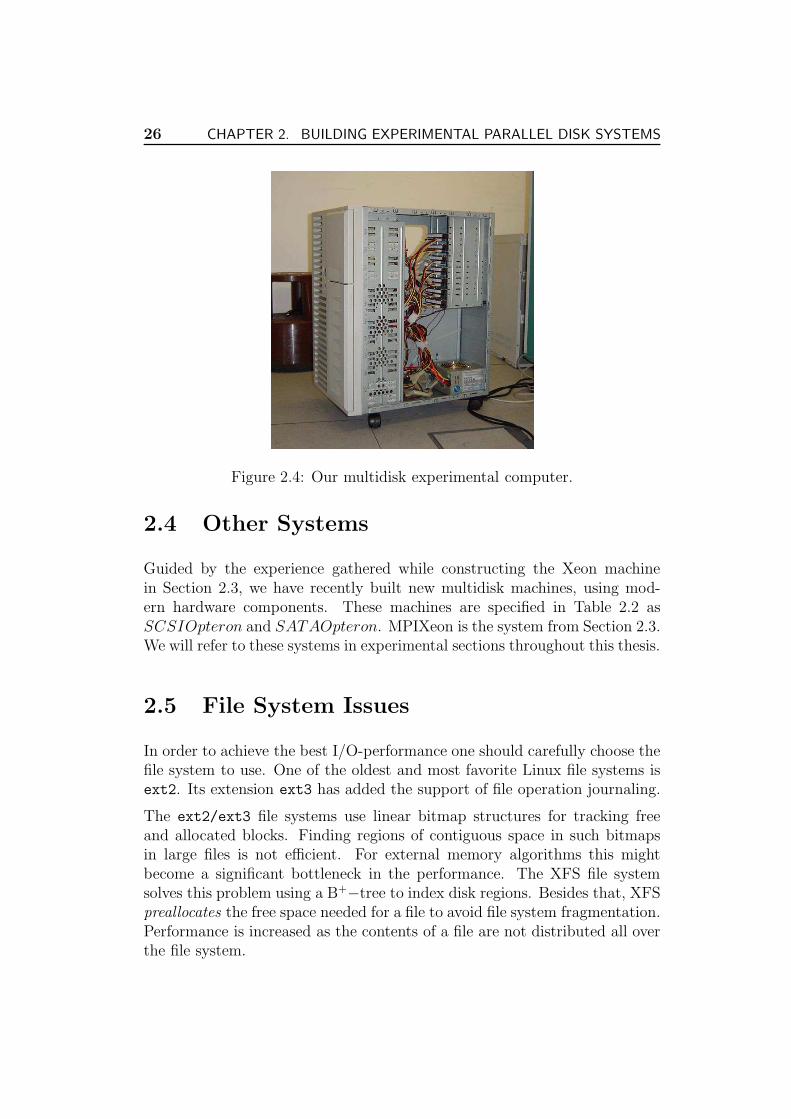
This high performance system cost only about 3000 Euro in 2002. Thelist with detailed information about the system components is presented inTable 2.1. The photograph of the computer is shown in Figure 2.4.
Table 2.1: Hardware components of our experimental computer.
Item # Euro/ItemMotherboard SUPER P4DP6 1 400Xeon 2.0 GHz processor 2 400IBM IC35L080AVVA07 80 GB disk 9 100Promise Ultra133 TX2 parallel ATA controller 5 35512 MB DDR2 memory 2 200Case/chassis 1 400
26 CHAPTER 2. BUILDING EXPERIMENTAL PARALLEL DISK SYSTEMS
Figure 2.4: Our multidisk experimental computer.
2.4 Other Systems
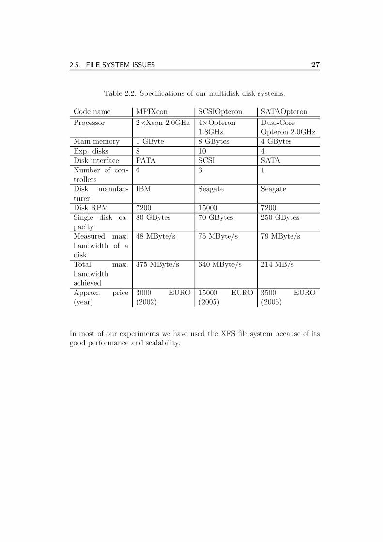
Guided by the experience gathered while constructing the Xeon machinein Section 2.3, we have recently built new multidisk machines, using mod-ern hardware components. These machines are specified in Table 2.2 asSCSIOpteron and SATAOpteron. MPIXeon is the system from Section 2.3.We will refer to these systems in experimental sections throughout this thesis.
2.5 File System Issues
In order to achieve the best I/O-performance one should carefully choose thefile system to use. One of the oldest and most favorite Linux file systems isext2. Its extension ext3 has added the support of file operation journaling.
The ext2/ext3 file systems use linear bitmap structures for tracking freeand allocated blocks. Finding regions of contiguous space in such bitmapsin large files is not efficient. For external memory algorithms this mightbecome a significant bottleneck in the performance. The XFS file systemsolves this problem using a B+−tree to index disk regions. Besides that, XFSpreallocates the free space needed for a file to avoid file system fragmentation.Performance is increased as the contents of a file are not distributed all overthe file system.
2.5. FILE SYSTEM ISSUES 27
Table 2.2: Specifications of our multidisk disk systems.
Code name MPIXeon SCSIOpteron SATAOpteron
Processor 2×Xeon 2.0GHz 4×Opteron1.8GHz
Dual-CoreOpteron 2.0GHz
Main memory 1 GByte 8 GBytes 4 GBytesExp. disks 8 10 4Disk interface PATA SCSI SATANumber of con-trollers
6 3 1
Disk manufac-turer
IBM Seagate Seagate
Disk RPM 7200 15000 7200Single disk ca-pacity
80 GBytes 70 GBytes 250 GBytes
Measured max.bandwidth of adisk
48 MByte/s 75 MByte/s 79 MByte/s
Total max.bandwidthachieved
375 MByte/s 640 MByte/s 214 MB/s
Approx. price(year)
3000 EURO(2002)
15000 EURO(2005)
3500 EURO(2006)
In most of our experiments we have used the XFS file system because of itsgood performance and scalability.

28 CHAPTER 2. BUILDING EXPERIMENTAL PARALLEL DISK SYSTEMS
Chapter 3
The Stxxl Library
The material covered in this chapter has been published partially in [DKS05a,DKS05b, DS03].
3.1 Stxxl Design
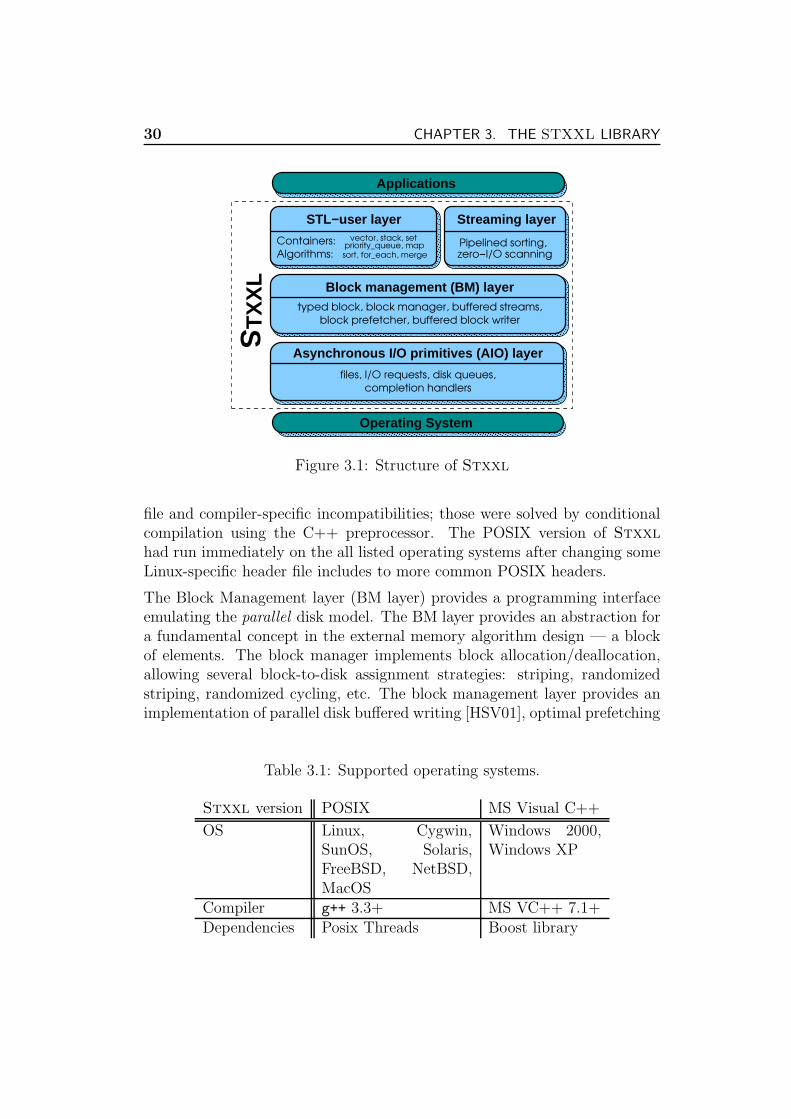
Stxxl is a layered library consisting of three layers (see Figure 3.1). Thelowest layer, the Asynchronous I/O primitives layer (AIO layer), abstractsaway the details of how asynchronous I/O is performed on a particular oper-ating system. Other existing external memory algorithm libraries only relyon synchronous I/O APIs [CM99] or allow reading ahead sequences storedin a file using the POSIX asynchronous I/O API [ABH+03]. These librariesalso rely on uncontrolled operating system I/O caching and buffering in or-der to overlap I/O and computation in some way. However, this approachhas significant performance penalties for accesses without locality. Unfortu-nately, the asynchronous I/O APIs are very different for different operatingsystems (e.g. POSIX AIO and Win32 Overlapped I/O). Therefore, we haveintroduced the AIO layer to make porting Stxxl easy. Porting the wholelibrary to a different platform requires only reimplementing the AIO layerusing native file access methods and/or native multithreading mechanisms.
Stxxl already has several implementations of the AIO layer which use dif-ferent file access methods under POSIX/UNIX and Windows systems (seeTable 3.1). Porting Stxxl to Windows took only a few days. The mainefforts were spent for writing the AIO layer using the native Windows calls.Rewriting the thread-related code was easy provided the Boost thread li-brary; its interfaces are similar to POSIX threads. There were little header
29
30 CHAPTER 3. THE STXXL LIBRARY
TX
XL
S
files, I/O requests, disk queues,
block prefetcher, buffered block writer
completion handlers
Block management (BM) layertyped block, block manager, buffered streams,
Containers:
STL−user layervector, stack, set
priority_queue, mapsort, for_each, merge
Pipelined sorting,zero−I/O scanning
Streaming layer
Algorithms:
Operating System
Applications
Asynchronous I/O primitives (AIO) layer
Figure 3.1: Structure of Stxxl
file and compiler-specific incompatibilities; those were solved by conditionalcompilation using the C++ preprocessor. The POSIX version of Stxxl
had run immediately on the all listed operating systems after changing someLinux-specific header file includes to more common POSIX headers.
The Block Management layer (BM layer) provides a programming interfaceemulating the parallel disk model. The BM layer provides an abstraction fora fundamental concept in the external memory algorithm design — a blockof elements. The block manager implements block allocation/deallocation,allowing several block-to-disk assignment strategies: striping, randomizedstriping, randomized cycling, etc. The block management layer provides animplementation of parallel disk buffered writing [HSV01], optimal prefetching
Table 3.1: Supported operating systems.
Stxxl version POSIX MS Visual C++
OS Linux, Cygwin,SunOS, Solaris,FreeBSD, NetBSD,MacOS
Windows 2000,Windows XP
Compiler g++ 3.3+ MS VC++ 7.1+Dependencies Posix Threads Boost library

3.1. STXXL DESIGN 31
[HSV01], and block caching. The implementations are fully asynchronousand designed to explicitly support overlapping between I/O and computation.
The top of Stxxl consists of two modules. The STL-user layer providesexternal memory sorting, external memory stack, external memory priorityqueue, etc. which have (almost) the same interfaces (including syntax andsemantics) as their STL counterparts. The Streaming layer provides efficientsupport for pipelining external memory algorithms. Many external memoryalgorithms, implemented using this layer, can save a factor of 2–3 in I/Os.For example, the algorithms for external memory suffix array constructionimplemented with this module [DMKS05] require only 1/3 of the numberof I/Os which must be performed by implementations that use conventionaldata structures and algorithms (either from Stxxl STL-user layer, LEDA-SM, or TPIE). The win is due to an efficient interface that couples the inputand the output of the algorithm–components (scans, sorts, etc.). The outputfrom an algorithm is directly fed into another algorithm as input, withoutneeding to store it on the disk in-between. This generic pipelining interfaceis the first of this kind for external memory algorithms.
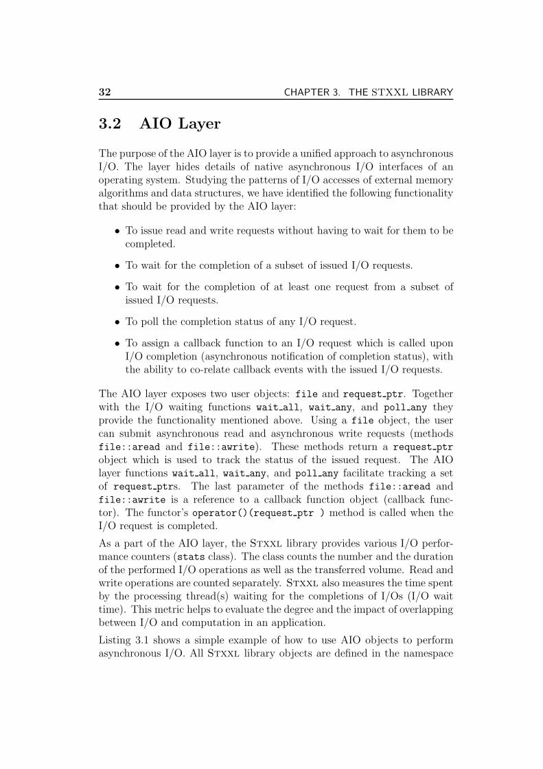
32 CHAPTER 3. THE STXXL LIBRARY
3.2 AIO Layer
The purpose of the AIO layer is to provide a unified approach to asynchronousI/O. The layer hides details of native asynchronous I/O interfaces of anoperating system. Studying the patterns of I/O accesses of external memoryalgorithms and data structures, we have identified the following functionalitythat should be provided by the AIO layer:
• To issue read and write requests without having to wait for them to becompleted.
• To wait for the completion of a subset of issued I/O requests.
• To wait for the completion of at least one request from a subset ofissued I/O requests.
• To poll the completion status of any I/O request.
• To assign a callback function to an I/O request which is called uponI/O completion (asynchronous notification of completion status), withthe ability to co-relate callback events with the issued I/O requests.
The AIO layer exposes two user objects: file and request ptr. Togetherwith the I/O waiting functions wait all, wait any, and poll any theyprovide the functionality mentioned above. Using a file object, the usercan submit asynchronous read and asynchronous write requests (methodsfile::aread and file::awrite). These methods return a request ptr
object which is used to track the status of the issued request. The AIOlayer functions wait all, wait any, and poll any facilitate tracking a setof request ptrs. The last parameter of the methods file::aread andfile::awrite is a reference to a callback function object (callback func-tor). The functor’s operator()(request ptr ) method is called when theI/O request is completed.
As a part of the AIO layer, the Stxxl library provides various I/O perfor-mance counters (stats class). The class counts the number and the durationof the performed I/O operations as well as the transferred volume. Read andwrite operations are counted separately. Stxxl also measures the time spentby the processing thread(s) waiting for the completions of I/Os (I/O waittime). This metric helps to evaluate the degree and the impact of overlappingbetween I/O and computation in an application.
Listing 3.1 shows a simple example of how to use AIO objects to performasynchronous I/O. All Stxxl library objects are defined in the namespace

3.2. AIO LAYER 33
stxxl. For convenience, in Line 1 we bring all names from the Stxxl
namespace to the local scope. In Line 9 a file object myfile is constructed.syscall file is an implementation of the Stxxl file interface which usesUNIX/POSIX read and write system calls to perform I/O. The file named"storage" in the current directory is opened in read-only mode. In Line 11an asynchronous read of the 1 MB region of the file starting at position 0 isissued. The data will be read into the array mybuffer. When the read oper-ation is completed, my handler::operator() will be called with a pointer tothe completed request. The execution stops at Line 13 waiting for the com-pletion of the issued read operation. Note that the work done in the functiondo something1() is overlapped with reading. When the I/O is finished, onecan process the read buffer (Line 14) and free it (Line 15).
Listing 3.1: Example of how to program with the AIO layer.
1 us ing namespace stxxl ;2 s t r u c t my_handler // I /O complet ion handler3 void operator ( ) ( request_ptr ptr ) 4 std : : cout << "Request ’"<< ∗ptr <<"’ completed."
5 <<std : : endl ;6 7 ;8 char ∗ mybuffer = new char [ 1 0 2 4∗ 1 0 2 4 ] ; // a l l o c a t e 1MB bu f f e r9 syscall_file myfile ("./storage" , file : : RDONLY ) ;
10 request_ptr myreq = myfile . aread ( mybuffer , 0 ,11 1024∗1024 , my_handler ( ) ) ;12 do_something1 ( ) ; // do something1 ( ) i s over lapped with read ing13 myreq−>wait ( ) ; //wait f o r read complet ion14 do_something2( mybuffer ) ; // pro ce s s the read bu f f e r15 de l e t e [ ] mybuffer ; // f r e e the bu f f e r
3.2.1 AIO Layer Implementations
There are several implementation strategies for the Stxxl AIO layer. Someasynchronous I/O related APIs (and underlying libraries implementing them)already exist. The most well known framework is POSIX AIO, which has animplementation on almost every UNIX/POSIX system. Its disadvantage isthat it has only limited support for I/O completion event mechanism 1. TheLinux AIO kernel side implementation 2 of POSIX AIO does not have thisdeficit, but is not portable since it works under Linux only.
1The Linux glibc implementation of POSIX AIO also has a performance drawback.It launches one user thread for each I/O operation. Stxxl starts one thread for each diskduring the library initialization, avoiding the thread start-up overhead for each I/O.
2http://freshmeat.net/projects/linux-aio/
34 CHAPTER 3. THE STXXL LIBRARY
The Stxxl AIO layer follows a different approach. It does not rely on anyasynchronous I/O API. Instead we use synchronous I/O calls running asyn-chronously in separate threads. For each file there is one read and one writerequest queue and one thread. The main thread posts requests (invokingfile::aread and file::awrite methods) to the file queues. The threadassociated with the file executes the requests in FIFO order. This approachis very flexible and it does not suffer from limitations of native asynchronousAPIs.
Our POSIX implementation of the AIO layer is based on POSIX threadsand supports several Unix file access methods: the syscall method usesread and write system calls, the mmap method uses memory mapping (mmapand munmap calls), the sim disk method simulates I/O timings of a harddisk provided a big internal memory. To avoid superfluous copying of databetween the user and kernel buffer memory, the syscall method has theoption to use unbuffered file system access. These file access methods canalso be used for raw disk I/O, bypassing the file system. In this case, insteadof files, raw device handles are open. The read/write calls using directaccess (O DIRECT option) have shown the best performance under Linux.The disadvantage of the mmap call is that programs using this method haveless control over I/O: In most operating systems 4 KBytes data pages of ammaped file region are brought to the main memory “lazily”, only when theyare accessed for the first time. This means if one mmaps a 100 KBytes blockand touches only the first and the last element of the block then two I/Osare issued by the operating system. This will slow down many I/O-efficientalgorithms, since for modern disks the seek time is much longer than thereading of 100 KBytes of contiguous data.
The POSIX implementation does not need to be ported to other UNIX com-patible systems, since POSIX threads is the standard threading API on allPOSIX-compatible operating systems.
Our Windows implementation is based on Boost threads, whose interfacesare very similar to POSIX threads.
AIO file and request implementation classes are derived from the genericfile and request interface classes with C++ pure virtual functions. Thesefunctions are specialized for each access method in implementation classesto define the read, write, wait for I/O completion and other operations. Thedesired access method implementation for a file is chosen dynamically at run-ning time. One can add the support of an additional access method (e.g. fora DAFS distributed filesystem) just providing classes implementing the fileand request interfaces. We have decided to use the virtual function mech-
3.2. AIO LAYER 35
anism in the AIO layer because this mechanism is very flexible and will notsacrifice the performance of the library, since the virtual functions of the AIOlayer need to be called only once per large chunk of data (i.e. B bytes). Theinefficiencies of C++ virtual functions are explained in Section 1.5. Similarto STL, the higher layers of Stxxl do not rely on the running time poly-morphism with virtual functions to avoid the high per–element penalties.
36 CHAPTER 3. THE STXXL LIBRARY
3.3 BM Layer
As already mentioned above, the BM layer provides an implementation ofthe central concept in I/O efficient algorithms and data structures: a block ofelements (typed block object). Besides, it includes a toolbox for allocating,deallocating, buffered writing, prefetching, and caching of blocks. The ex-ternal memory manager (object block manager) is responsible for allocatingand deallocating external memory space on disks. The manager supportsfour parallel disk allocation strategies: simple striping, fully randomized,simple randomized [BGV97], and randomized cycling [VH01].
The BM layer also delivers a set of helper classes that efficiently implementfrequently used sequential patterns of interaction with the (parallel disk)external memory. The optimal parallel disk queued writing [HSV01] is im-plemented in the buffered writer class. The class operates on blocks. Thebuf ostream class is build on top of buffered writer and has a high levelinterface, similar to the interface of STL output iterators. Analogously, theclasses block prefetcher and buf istream contain an implementation ofan optimal parallel disk prefetching algorithm [HSV01]. The helper objectsof the BM layer support overlapping between I/O and computation, whichmeans that they are able to perform I/O in the background, while the userthread is doing useful computations.
The BM layer views external memory as a set of large AIO files — one for eachdisk. We will refer to these files as disks. The other approach would be to mapa related subset of blocks (e. g. those belonging to the same data structure) toa separate file. This approach has some performance problems. One of themis that since those (numerous) files are created dynamically, during the run ofthe program, the file system allocates the disk space on demand, that mightin turn introduce severe uncontrolled disk space fragmentation. Thereforewe have chosen the “one-large-file-per-disk” approach as our major scheme.However, the design of our library does not forbid data structures to storetheir content in separate user data files (e.g., as an option, stxxl::vectorcan be mapped to a user file, see Section 3.4).
The external memory manager (object block manager) is responsible forallocating and deallocating external memory space on the disks. Theblock manager reads information about available disks from the Stxxl con-figuration file. This file contains the location of each disk file, the sizes ofthe disks, and the file access methods for each disk. When allocating abunch of blocks, a programmer can specify how the blocks will be assignedto disks, passing an allocation strategy function object. The block manager
implements the “first-fit” allocation heuristic [BS03]. When an application
3.3. BM LAYER 37
requests several blocks from a disk, the manager tries to allocate the blockscontiguously. This reduces the bulk access time. On allocation requests, theblock manager returns BID objects – Block IDentifiers. An object of thetype BID describes the physical location of an allocated block, including thedisk and offset of a region of storage on disk. One can load or store the datathat resides at the location given by the BID using asynchronous read andwrite methods of a typed block object.
The full signature of the Stxxl “block of elements” class istyped block<RawSize,T,NRef,InfoType>. The C++ template parameterRawSize defines the total size of the block in bytes. Since block size is not asingle global constant in Stxxl, a programmer can simultaneously operatewith several block types having different blocks sizes. Such flexibility is oftenrequired for good performance. For example, B+-tree leaves might have a sizedifferent from the size of the internal nodes. We have made the block sizea template parameter and not a member variable for the sake of efficiency.The values of the template parameters are known to the compiler, thereforefor the power of two values (a very common choice) it can replace many arith-metic operations, like divisions and multiplications, by more efficient binaryshifts. A critical requirement for many external memory data structures isthat a block must be able to store links to other blocks. An Stxxl block canstore NRef objects of type BID. Additionally, one can equip a block with afield of the type InfoType, that can hold some per-block information. Blockelements of type T can easily be accessed by the array operator [] and viarandom access iterators. The maximum number of elements available a blockdepends on the number of links and the sizes of T, InfoType and BID types.contains a This number is accessible as typed block<...>::size.
In Listing 3.2, we give an example of how to program block I/O using objectsof the BM layer. In Line 2 we define the type of block: its size is one megabyteand the type of elements is double. The pointer to the only instance of thesingleton object block manager is obtained in Line 5. Line 7 asks the blockmanager to allocate 32 blocks in external memory. The new blocks callwrites the allocated BIDs to the output iterator, given by the last parame-ter. The std::back inserter iterator adapter will insert the output BIDsat the end of the array bids. The manager assigns blocks to disks in a round-robin fashion as the striping() strategy suggests. Line 8 allocates 32 inter-nal memory blocks. The internal memory allocator new alloc<block type>
of Stxxl allocates blocks on a virtual memory page boundary, which isa requirement for unbuffered file access. Along lines 9–11 the elements ofblocks are filled with some values. Then, the blocks are submitted for writ-ing (lines 12–13). The request objects are stored in an std::vector for
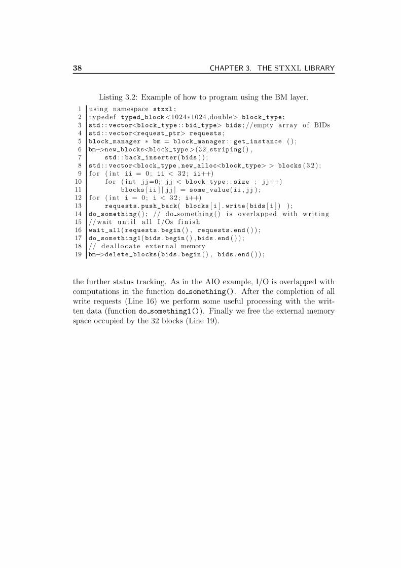
38 CHAPTER 3. THE STXXL LIBRARY
Listing 3.2: Example of how to program using the BM layer.
1 us ing namespace stxxl ;2 typede f typed_block<1024∗1024 ,double> block_type ;3 std : : vector<block_type : : bid_type> bids ; //empty ar ray o f BIDs4 std : : vector<request_ptr> requests ;5 block_manager ∗ bm = block_manager : : get_instance ( ) ;6 bm−>new_blocks<block_type>(32 ,striping ( ) ,7 std : : back_inserter( bids ) ) ;8 std : : vector<block_type , new_alloc<block_type> > blocks ( 3 2 ) ;9 f o r ( i n t ii = 0 ; ii < 32 ; ii++)
10 f o r ( i n t jj=0; jj < block_type : : size ; jj++)11 blocks [ ii ] [ jj ] = some_value(ii , jj ) ;12 f o r ( i n t i = 0 ; i < 32 ; i++)13 requests . push_back( blocks [ i ] . write ( bids [ i ] ) ) ;14 do_something ( ) ; // do something ( ) i s over lapped with wr i t ing15 //wait un t i l a l l I /Os f i n i s h16 wait_all( requests . begin ( ) , requests . end ( ) ) ;17 do_something1( bids . begin ( ) , bids . end ( ) ) ;18 // d e a l l o c a t e e x t e r na l memory19 bm−>delete_blocks( bids . begin ( ) , bids . end ( ) ) ;
the further status tracking. As in the AIO example, I/O is overlapped withcomputations in the function do something(). After the completion of allwrite requests (Line 16) we perform some useful processing with the writ-ten data (function do something1()). Finally we free the external memoryspace occupied by the 32 blocks (Line 19).

3.4. STL -USER LAYER 39
3.4 Stl -User Layer
When we started to develop the library we decided to equip our imple-mentations of external memory data structures and algorithms with wellknown generic interfaces of the Standard Template Library, which is a partof the C++ standard. This choice would shorten the application develop-ment times, since the time to learn new interfaces is saved. Porting aninternal memory code that relies on STL would also be easy, since interfacesof STL-user layer data structures (containers in the STL terminology) andalgorithms have the same syntax and semantics.
We go over the containers currently available in Stxxl.
3.4.1 Vector
The most universal Stxxl container is stxxl::vector. Vector is an arraywhose size can vary dynamically. The implementation of stxxl::vector issimilar to the LEDA-SM array [CM99]. The content of a vector is stripedblock-wise over the disks, using an assignment strategy given as a templateparameter. Some of the blocks are cached in a vector cache of fixed size (alsoa parameter). The replacement of cache blocks is controlled by a specifiedpage-replacement strategy. Stxxl has implementations of LRU and randomreplacement strategies. The user can provide his/her own strategy as well.The Stxxl vector has STL-compatible Random Access Iterators. Onerandom access costs O(1) I/Os in the worst case. Sequential scanning of thevector costs O(1/DB) amortized I/Os per vector element.
3.4.2 Stack
An I/O efficient stack is perhaps the simplest external memory data struc-ture. Four different implementations of a stack are available in Stxxl. Someof the implementations (e.g. stxxl::grow shrink stack2) are optimized toprefetch data ahead and to queue writing, efficiently overlapping I/O andcomputation. The amortized I/O complexity for push and pop stack opera-tions is O(1/DB).
We compare the performance of Stxxl stack with performance of LEDA-SM and TPIE stacks in a simple test: we insert records to the stacks andafterwards delete them all. We try 4- and 32-byte records to evaluate differentCPU processing overheads. The used experimental system had a 3.00 GHzPentium 4 processor, 1 GB of main memory and a SATA disk dedicated to the
40 CHAPTER 3. THE STXXL LIBRARY
experiments. The measured maximum I/O bandwidth of the hard disk was72 MB/s for writing and 65 MByte/s for reading. Before the insertion, weallocated a 768 MByte array and filled it with zeros to prevent this memoryto be used for file system buffering, which would distort the measurements.This also simulates the memory consumption of other algorithms and datastructures used in a real application. The rest of the memory was used forbuffer blocks for stacks in the libraries and for operating system buffers in thecase of LEDA-SM and TPIE. Stxxl has used its own buffer and prefetchingmechanism. The block size was set to two MBytes. Preliminary experimentshave shown that larger blocks did not help any of the libraries. The LEDA-SM implementation could only be compiled with the g++ compiler version2.95. Stxxl and TPIE implementations have been compiled with g++ 3.3.The compiler optimization level was set to -O3 for both codes.
Figures 3.2–3.5 show the bandwidth achieved in the experiments, which wascomputed as n · sizeof(T)/t, where n is the number of elements to in-sert/delete, T is the data type and t is the time to insert/delete all n ele-ments. The experiments were conducted on input volumes of 1-8 GBytes.Since we have only registered insignificant variations, the average bandwidthsare presented. We considered the following stack implementations (from leftto right in Figures 3.2–3.5):
• Stxxl grow shrink stack2 (GS2) using block pools for asynchronousprefetching and buffering. The name of this stack stems from the ac-cess pattern it supports with the best efficiency: An empty stack is firstfilled with elements up to the maximum number of elements and thenall elements are removed one after another. In the first step the imple-mentation is operating in the “grow” mode, using a pool of blocks forbuffering the incoming elements. In the second step it is operating inthe “shrink” mode, reading ahead some number of blocks (user-definedvalue) using a prefetch block pool. This type of access (or similar) is fre-quently used in applications, see e.g. Section 4.3. grow shrink stack2
and grow shrink stack1 implementations differ in the usage mode ofthe block pools: the former uses pools, shared between (possibly) sev-eral Stxxl data structures, the latter has an exclusive access to itsown pools.
• Stxxl normal stack is a classical implementation with synchronousreading and writing,
• LEDA-SM stack implementation,
• TPIE stack implementation using the mmap function for disk access,
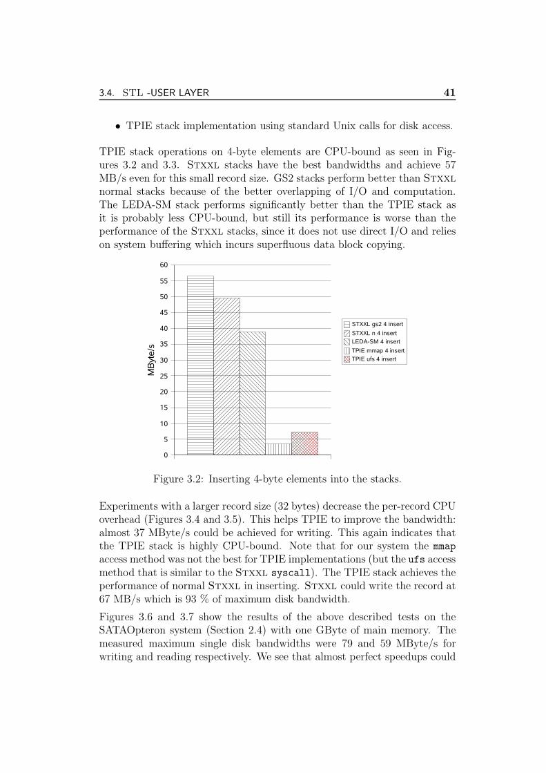
3.4. STL -USER LAYER 41
• TPIE stack implementation using standard Unix calls for disk access.
TPIE stack operations on 4-byte elements are CPU-bound as seen in Fig-ures 3.2 and 3.3. Stxxl stacks have the best bandwidths and achieve 57MB/s even for this small record size. GS2 stacks perform better than Stxxl
normal stacks because of the better overlapping of I/O and computation.The LEDA-SM stack performs significantly better than the TPIE stack asit is probably less CPU-bound, but still its performance is worse than theperformance of the Stxxl stacks, since it does not use direct I/O and relieson system buffering which incurs superfluous data block copying.
0
5
10
15
20
25
30
35
40
45
50
55
60
STXXL gs2 4 insert
STXXL n 4 insert
LEDA-SM 4 insert
TPIE mmap 4 insert
TPIE ufs 4 insert
MB
yte
/s
Figure 3.2: Inserting 4-byte elements into the stacks.
Experiments with a larger record size (32 bytes) decrease the per-record CPUoverhead (Figures 3.4 and 3.5). This helps TPIE to improve the bandwidth:almost 37 MByte/s could be achieved for writing. This again indicates thatthe TPIE stack is highly CPU-bound. Note that for our system the mmap
access method was not the best for TPIE implementations (but the ufs accessmethod that is similar to the Stxxl syscall). The TPIE stack achieves theperformance of normal Stxxl in inserting. Stxxl could write the record at67 MB/s which is 93 % of maximum disk bandwidth.
Figures 3.6 and 3.7 show the results of the above described tests on theSATAOpteron system (Section 2.4) with one GByte of main memory. Themeasured maximum single disk bandwidths were 79 and 59 MByte/s forwriting and reading respectively. We see that almost perfect speedups could
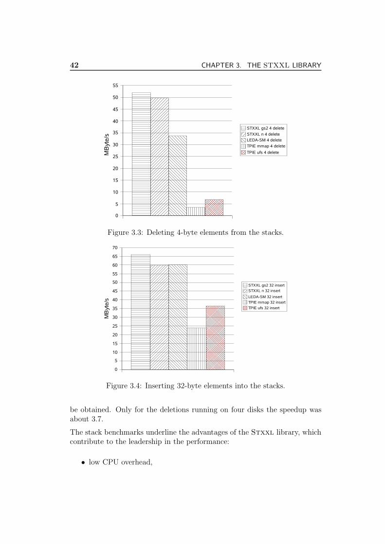
42 CHAPTER 3. THE STXXL LIBRARY
0
5
10
15
20
25
30
35
40
45
50
55
STXXL gs2 4 delete
STXXL n 4 delete
LEDA-SM 4 delete
TPIE mmap 4 delete
TPIE ufs 4 deleteMB
yte/s
Figure 3.3: Deleting 4-byte elements from the stacks.
0
5
10
15
20
25
30
35
40
45
50
55
60
65
70
STXXL gs2 32 insert
STXXL n 32 insert
LEDA-SM 32 insert
TPIE mmap 32 insert
TPIE ufs 32 insert
MB
yte/s
Figure 3.4: Inserting 32-byte elements into the stacks.
be obtained. Only for the deletions running on four disks the speedup wasabout 3.7.
The stack benchmarks underline the advantages of the Stxxl library, whichcontribute to the leadership in the performance:
• low CPU overhead,

3.4. STL -USER LAYER 43
0
5
10
15
20
25
30
35
40
45
50
55
STXXL gs2 32 delete
STXXL n 32 delete
LEDA-SM 32 delete
TPIE mmap 32 delete
TPIE ufs 32 delete
MB
yte/s
Figure 3.5: Deleting 32-byte elements from the stacks.
0
25
50
75
100
125
150
175
200
225
250
275
D=1 gs2 4 insert
D=1 gs2 32 insert
D=2 gs2 4 insert
D=2 gs2 32 insert
D=4 gs2 4 insert
D=4 gs2 32 insert
MB
yte/s
Figure 3.6: Inserting elements into GS2 stacks (multiple disks).
• use of direct I/O to avoid unneeded data copying,
• use of own prefetching/buffering mechanisms for overlapping I/O andcomputation,
• support of parallel disks.

44 CHAPTER 3. THE STXXL LIBRARY
0
10
20
30
40
50
70
80
90
100
110
120
130
140
150
160
170
D=1 gs2 4 delete
D=1 gs2 32 delete
D=2 gs2 4 delete
D=2 gs2 32 delete
D=4 gs2 4 delete
D=4 gs2 32 delete
MB
yte/s
Figure 3.7: Deleting elements from GS2 stacks (multiple disks).
The source code of all stack tests described above is distributed with theStxxl library.
3.4.3 Queue
Stxxl also has an implementation of external memory FIFO queue. Its de-sign is similar to stxxl::grow shrink stack2. The implementation holdsthe head and the tail blocks in the main memory. Prefetch and write blockpools might be used to overlap I/O and computation during queue opera-tions.
3.4.4 Deque
The Stxxl implementation of external memory deque is an adaptor of an(external memory) vector. This implementation wraps the elements aroundthe end of the vector circularly. It provides the pop/push operations from/tothe both ends of the deque in O(1/DB) amortized I/Os if parameterized witha properly configured stxxl::vector.

3.4. STL -USER LAYER 45
3.4.5 Priority Queue
External memory priority queues are the central data structures for many I/Oefficient graph algorithms [Zeh02, CGG+95, MSS03]. The main technique inthese algorithms is time-forward processing [CGG+95, Arg95], easily realiz-able by an I/O efficient priority queue. I/O efficient priority queues also findapplication in large-scale discrete event simulation and online sorting. TheStxxl implementation of priority queues is based on [San00]. An operationof this priority queue, called sequence heap, takes O
(
1B
logM/B(I/B))
amor-tized I/Os, where I is the total number of insertions into the priority queue.This queue needs less than a third of I/Os used by other similar cache (I/O)efficient priority queues (e.g. [BCFM00, FJKT97]).
A sequence heap maintains R merge groups G1,. . ., GR where Gi holds upto k sorted sequences of size up to mki−1, m << M , see Figure 3.8. Whengroup Gi overflows, all its sequences are merged, and the resulting sequenceis put into group Gi+1. Each group is equipped with a group buffer of size mto allow batched deletion from the sequences. The smallest elements of thesebuffers are deleted in small batches and stored in the deletion buffer. Theelements are first inserted into the insertion priority queue. On deletion, onechecks the minimum elements stored in the insertion priority queue and thedeletion buffer.
The difference of our implementation to [San00] is that a number of largermerge groups are explicitly kept in external memory. The sorted sequencesin those groups only hold their first blocks in the main memory. The imple-mentation supports parallel disks and overlaps I/O and computation. As in[San00], the internal merging is based on loser trees [Knu98]. However, ourimplementation does not use sentinel elements.
In the following we compare the performance of the Stxxl priorityqueue with the general-purpose array heap implementation of LEDA-SM[BCFM00]. TPIE does not provide an I/O-efficient priority queue in thedistributed library version. We run the implementation on synthetic inputsfollowing [BCFM00]. The comparison of the data structures in a real graphalgorithm is presented in Section 4.2, where we implement an I/O-efficientmaximal independent set algorithm.
The first test performs n insertions, followed by n delete-min operations. Theelements inserted are pairs of key data 4-byte integers drawn randomly fromthe range [0, 231 − 1]. Figure 3.9 shows the running time of this experimentrunning on a system with a 3.00 GHz Pentium 4 processor, 1 GB of mainmemory and a SATA disk dedicated to the experiments. The priority queues

46 CHAPTER 3. THE STXXL LIBRARY
Figure 3.8: The structure of Stxxl priority queue.
were given 512 MB of main memory at their disposal, the rest was used by theLinux operating system for buffering in the case of LEDA-SM and for prefetchand write pools in the case of Stxxl . The LEDA-SM implementation couldonly be compiled with the g++ compiler version 2.95. Stxxl implementationwas compiled with g++ 3.3. The compiler optimization level was set to -O3
for both codes. We have tuned the external memory block size (256 KB) forLEDA-SM to obtain the best running times for the array heap. However, thedifferences in running times with different block sizes were negligible, which isa symptom of its CPU-boundness. The Stxxl priority queue used 2 MByteblocks. Note the drop of the LEDA-SM delete curve after n = 223 is not anartifact of the measurements; it has been also reported in the original study[BCFM00]. However, we do not devote much attention to the results withn ≤ 224 since those inputs fit in the internal memory. LEDA-SM containerscannot hold more than 231 −1 items, therefore we have stopped at input sizen = 2000 · 220, which corresponds to about 16 GByte of data. This input is
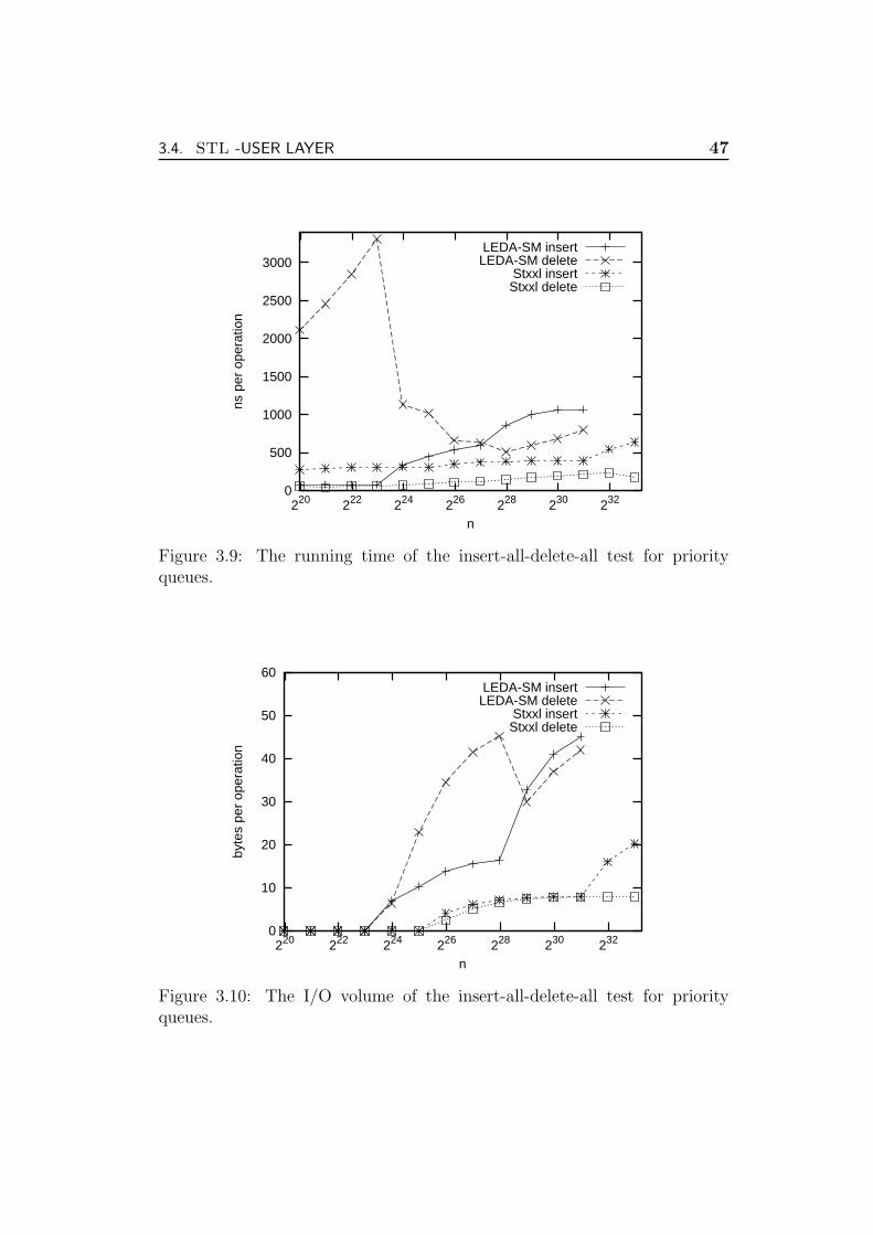
3.4. STL -USER LAYER 47
0
500
1000
1500
2000
2500
3000
232230228226224222220
ns p
er o
pera
tion
n
LEDA-SM insertLEDA-SM delete
Stxxl insertStxxl delete
Figure 3.9: The running time of the insert-all-delete-all test for priorityqueues.
0
10
20
30
40
50
60
232230228226224222220
byte
s pe
r op
erat
ion
n
LEDA-SM insertLEDA-SM delete
Stxxl insertStxxl delete
Figure 3.10: The I/O volume of the insert-all-delete-all test for priorityqueues.
48 CHAPTER 3. THE STXXL LIBRARY
32 times larger than the main memory size and it is reasonable to be handledin external memory. The Stxxl priority queue is up to 2.7 times and 3.7times faster for insertions and deletions respectively. This can be explainedby more expensive CPU work taking place in the LEDA-SM implementationand also better explicit overlapping of I/O and computation of Stxxl. Notethat LEDA-SM relies on (general purpose) operating system caching andbuffering. The insertion and deletion phases for the Stxxl priority queueneed almost the same number of I/Os for n ≤ 231. The insertion phase hasalso the advantage that writing is faster than reading, nonetheless it is almosttwo times slower than the deletion phase. This is explained by the higherCPU work needed for merging and filling the buffers during insertions. Theinsertion phase is highly CPU-bound which is confirmed by the I/O-waittime counter, whose value was close to zero. According to the I/O-wait timecounter, the deletion phase is less CPU-bound. For n ≥ 232 the insertionphase needs to merge and insert external sequences, which implies moreI/O operations and results in the observed running time escalation. This isconfirmed by Figure 3.10, which also shows that the I/O volume of Stxxl
priority queue is 2–5.5 times smaller than the I/O volume of the LEDA-SMarray heap. This difference has been predicted in the original paper [San00].
Figure 3.11 presents the running times of another synthetic test: we insert nrandom elements into the priority queues and then measure the running timeof n operations: We insert a random pair with probability 1
3and delete the
minimum with probability 23. The behavior of the LEDA-SM curve is similar
to the deletions. The Stxxl curve has two steps: The first step occurs whenthe internal sequences have to be merged and put into the external memoryfor the first time (n = 225), the next step happens at n = 231 when sequencesfrom the first external merger have to be merged and put into a sequenceof the second external merger for the first time (see Figure 3.12). Thesesteps are hardly seen in Figure 3.9 (insertions) because of the different accesspattern and amortization (n versus 4n
3insertions).
Figures 3.13, 3.14 and 3.15 show the results of the above described tests on asystem with a 2.0 GHz Opteron Dual-Core Processor and one GByte of mainmemory and four IDE hard disks (SATAOpteron system from Section 2.4).We could not run LEDA-SM since it compiles only with the old g++ 2.95
compiler, available only for 32-bit architectures. One can see that insertionsare highly CPU-bound till n = 231 and cannot benefit from disk parallelism(we ran the implementation on 1,2 and 4 identical independent disks). Also,for larger inputs, where large external sequences have to be merged morefrequently, we could not achieve a speedup larger than 1.4 for four disks,because of the CPU-boundness. The delete operation is less CPU-expensive,

3.4. STL -USER LAYER 49
0
500
1000
1500
2000
2500
232230228226224222220
ns p
er o
pera
tion
n
LEDA-SMStxxl
Figure 3.11: The running times of intermixed insertions with deletions (pri-ority queues).
0
10
20
30
40
50
232230228226224222220
byte
s pe
r op
erat
ion
n
LEDA-SMStxxl
Figure 3.12: The I/O volume of intermixed insertions with deletions (priorityqueues).

50 CHAPTER 3. THE STXXL LIBRARY
therefore we can already see a small speedup for n ≥ 227 (Figure 3.14). Thesteps in the running time in Figure 3.15 are more prominent compared toFigure 3.11 because the I/O plays a greater role on the faster 64-bit OpteronCPU.
0
100
200
300
400
500
600
700
234232230228226224222220
ns p
er o
pera
tion
n
Stxxl insert D=1Stxxl insert D=2Stxxl insert D=4
Figure 3.13: Insertions (priority queue with multiple disks).
0
50
100
150
200
250
234232230228226224222220
ns p
er o
pera
tion
n
Stxxl delete D=1Stxxl delete D=2Stxxl delete D=4
Figure 3.14: Deletions (priority queue with multiple disks).
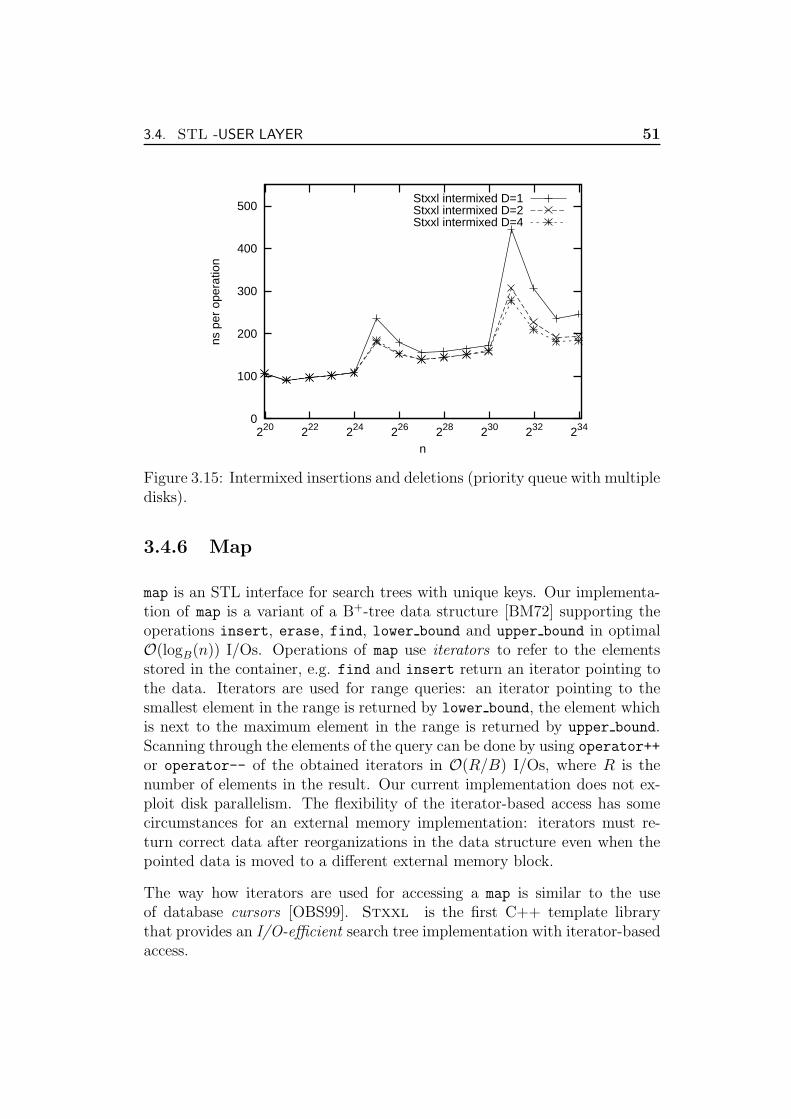
3.4. STL -USER LAYER 51
0
100
200
300
400
500
234232230228226224222220
ns p
er o
pera
tion
n
Stxxl intermixed D=1Stxxl intermixed D=2Stxxl intermixed D=4
Figure 3.15: Intermixed insertions and deletions (priority queue with multipledisks).
3.4.6 Map
map is an STL interface for search trees with unique keys. Our implementa-tion of map is a variant of a B+-tree data structure [BM72] supporting theoperations insert, erase, find, lower bound and upper bound in optimalO(logB(n)) I/Os. Operations of map use iterators to refer to the elementsstored in the container, e.g. find and insert return an iterator pointing tothe data. Iterators are used for range queries: an iterator pointing to thesmallest element in the range is returned by lower bound, the element whichis next to the maximum element in the range is returned by upper bound.Scanning through the elements of the query can be done by using operator++
or operator-- of the obtained iterators in O(R/B) I/Os, where R is thenumber of elements in the result. Our current implementation does not ex-ploit disk parallelism. The flexibility of the iterator-based access has somecircumstances for an external memory implementation: iterators must re-turn correct data after reorganizations in the data structure even when thepointed data is moved to a different external memory block.
The way how iterators are used for accessing a map is similar to the useof database cursors [OBS99]. Stxxl is the first C++ template librarythat provides an I/O-efficient search tree implementation with iterator-basedaccess.
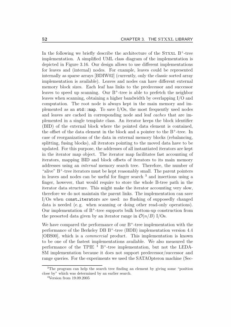
52 CHAPTER 3. THE STXXL LIBRARY
In the following we briefly describe the architecture of the Stxxl B+-treeimplementation. A simplified UML class diagram of the implementation isdepicted in Figure 3.16. Our design allows to use different implementationsfor leaves and (internal) nodes. For example, leaves could be representedinternally as sparse arrays [BDIW02] (currently, only the classic sorted arrayimplementation is available). Leaves and nodes can have different externalmemory block sizes. Each leaf has links to the predecessor and successorleaves to speed up scanning. Our B+-tree is able to prefetch the neighborleaves when scanning, obtaining a higher bandwidth by overlapping I/O andcomputation. The root node is always kept in the main memory and im-plemented as an std::map. To save I/Os, the most frequently used nodesand leaves are cached in corresponding node and leaf caches that are im-plemented in a single template class. An iterator keeps the block identifier(BID) of the external block where the pointed data element is contained,the offset of the data element in the block and a pointer to the B+-tree. Incase of reorganizations of the data in external memory blocks (rebalancing,splitting, fusing blocks), all iterators pointing to the moved data have to beupdated. For this purpose, the addresses of all instantiated iterators are keptin the iterator map object. The iterator map facilitates fast accounting ofiterators, mapping BID and block offsets of iterators to its main memoryaddresses using an internal memory search tree. Therefore, the number of“alive” B+-tree iterators must be kept reasonably small. The parent pointersin leaves and nodes can be useful for finger search 3 and insertions using afinger, however, that would require to store the whole B-tree path in theiterator data structure. This might make the iterator accounting very slow,therefore we do not maintain the parent links. The implementation can saveI/Os when const iterators are used: no flushing of supposedly changeddata is needed (e. g. when scanning or doing other read-only operations).Our implementation of B+-tree supports bulk bottom-up construction fromthe presorted data given by an iterator range in O(n/B) I/Os.
We have compared the performance of our B+-tree implementation with theperformance of the Berkeley DB B+-tree (BDB) implementation version 4.4[OBS00], which is a commercial product. This implementation is knownto be one of the fastest implementations available. We also measured theperformance of the TPIE 4 B+-tree implementation, but not the LEDA-SM implementation because it does not support predecessor/successor andrange queries. For the experiments we used the SATAOpteron machine (Sec-
3The program can help the search tree finding an element by giving some “positionclose by” which was determined by an earlier search.
4Version from 19.09.2005

3.4.
ST
L-U
SER
LAY
ER
53 B T r e e h e i g h t : i n t+ i n s e r t ( v : V a l u e ) : I t e r a t o r+ e r a s e ( k : K e y ) : i n t+ f i n d ( k : K e y ) : I t e r a t o r+ l o w e r _ b o u n d ( k : K e y ) : I t e r a t o r
N o d e m e : B I D s i z e : i n t+ f i n d ( k : K e y , h : i n t ) : I t e r a t o r+ l o w e r _ b o u n d ( k : K e y , h : i n t ) : I t e r a t o r+ i n s e r t ( v : V a l u e , h : i n t , o u t s : S p l i t t e r ) : I t e r a t o r+ e r a s e ( k : K e y , h : i n t )
L e a f m e : B I D p r e d : B I D s u c c : B I D s i z e : i n t+ f i n d ( k : K e y ) : I t e r a t o r+ i n c r e m e n t ( i n o u t i : I t e r a t o r )+ d e c r e m e n t ( i n o u t i : I t e r a t o r )+ l o w e r _ b o u n d ( k : K e y ) : I t e r a t o r+ i n s e r t ( v : V a l u e , o u t s : S p l i t t e r ) : I t e r a t o r+ e r a s e ( k : K e y )
N o d e C a c h e n o d e s : A r r a y B I D 2 i n t : M a p p a g e r : P a g e r f r e e N o d e s : L i s t+ g e t N o d e ( b : B I D ) : N o d e+ g e t N e w N o d e ( o u t b : B I D ) : L e a f+ d e l e t e L e a f ( b : B I D )+ f i x N o d e ( b : B I D )+ u n f i x N o d e ( b : B I D )
L e a f C a c h e+ g e t L e a f ( b : B I D ) : L e a f+ p r e f e t c h ( b : B I D )+ g e t N e w L e a f ( o u t b : B I D ) : L e a f+ d e l e t e L e a f ( b : B I D )
R o o t N o d e+ i n s e r t ( k : K e y , b : B I D )+ e r a s e ( k : K e y )+ f i n d ( k : K e y ) : B I DI t e r a t o r M a p+ r e g i s t e r ( i : I t e r a t o r )+ u n r e g i s t e r ( i : I t e r a t o r )+ f i n d ( b : B I D , p o s : i n t ) : I t e r a t o rI t e r a t o r+ I t e r a t o r ( )# I t e r a t o r ( i m : I t e r a t o r M a p , b : B I D , o : i n t )
S p l i t t e r k : K e y b : B I D
Figure 3.16: The simplified UML class diagram of the B+-tree implementation.

54 CHAPTER 3. THE STXXL LIBRARY
tion 2.4) using one GByte of main memory. Each implementation used aseparate hard disk for storing its external memory back file. Stxxl mapand TPIE have used a cache of 750 MBytes and BDB’s cache was slightlyless because it has used more memory than the given cache size 5. The blocksize was set to 32 KBytes for all implementations.
The B+-trees indexed records with eight character random keys (letters ’a’-’z’) and 32 bytes data field. First, B+-trees have been constructed from asorted set of n records. To make the comparison fair we configured BDB tostore records with unique keys, since the map interface does keep multiplerecords with equal keys. Stxxl map supports the bottom up bulk con-struction from a sorted range of iterators. TPIE B+-tree supports the bulkconstruction from a pre-sorted TPIE stream of data which must reside on ahard disk (AMI STREAM). According to the Berkeley DB support team, BDBlacks the bulk load capability, therefore we had to insert the records one byone in ascending order. This insertion pattern leads to nearly 100 % cachehits and produces a BDB B+-tree with a fill factor of about 100 % in theleaves. The stxxl::map and the TPIE bulk construction were configured toachieve the 100 % fill factor, too. Figure 3.17 shows the construction timewithout the pre-sorting. In this test, Stxxl map is about three times fasterthan BDB. The obvious reason for this is that BDB has to do many searchesin the leaves and nodes to find an appropriate place to insert, and thus ishighly CPU bound. Stxxl map bulk construction performs only a smallconstant number of operations per input element. The TPIE bulk construc-tion was up to 70 % slower than the construction of the stxxl::map, because,in fact, it repeatedly inserts all input elements into the leaves doing a binarysearch of the place to insert them into the last leaf over and over from thescratch. This inefficiency makes the construction more CPU-bound.
After the construction of the base element set index we generated 100,000random records and inserted them. The running times of this experimentare shown in Figure 3.18. For large inputs one has to load up to two leavesand flush up to three leaves per insertion since the leaves are full after theconstruction and they need to be split. Note that the links between theleaves must be updated, too. This can explain the long 25 ms of the Stxxl
and TPIE B+-trees since a random access to this hard disk takes up to 8 mson average according to its specifications paper. BDB is about 30% fasterfor large inputs; this advantage could to some extent be due to the adap-tive compression of sequences of keys with the same prefix, an optimizationexploited in the recent versions of BDB. Another reason would be a highly
5The BDB process has been killed by an out-of-memory exception when run with 750MByte cache. Therefore we had to reduce the cache size.
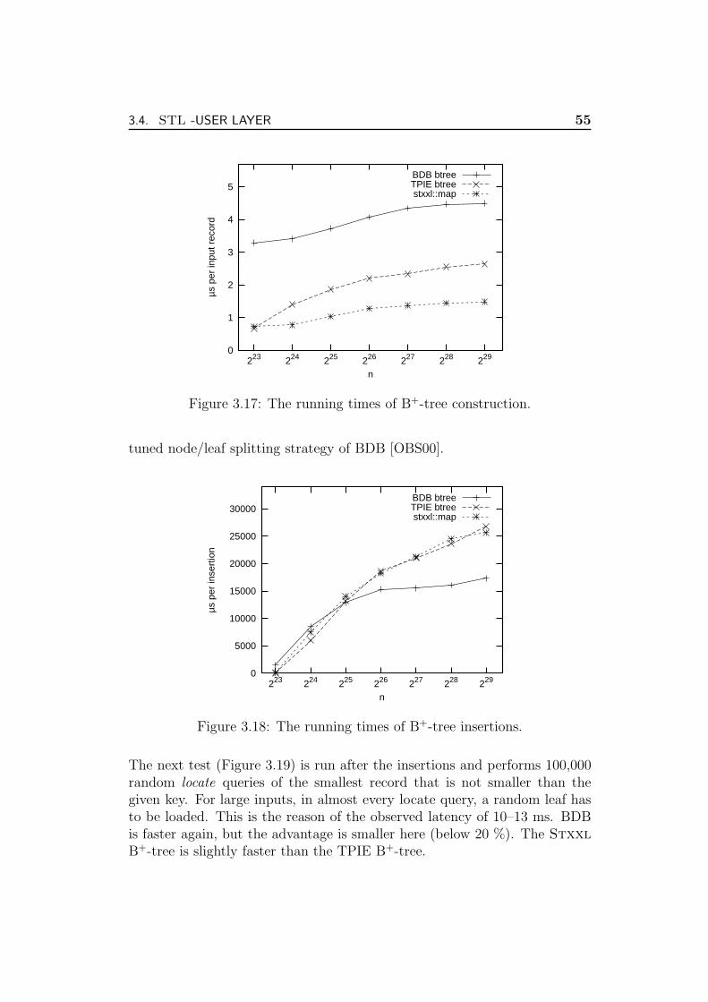
3.4. STL -USER LAYER 55
0
1
2
3
4
5
229228227226225224223
µs p
er in
put r
ecor
d
n
BDB btreeTPIE btreestxxl::map
Figure 3.17: The running times of B+-tree construction.
tuned node/leaf splitting strategy of BDB [OBS00].
0
5000
10000
15000
20000
25000
30000
229228227226225224223
µs p
er in
sert
ion
n
BDB btreeTPIE btreestxxl::map
Figure 3.18: The running times of B+-tree insertions.
The next test (Figure 3.19) is run after the insertions and performs 100,000random locate queries of the smallest record that is not smaller than thegiven key. For large inputs, in almost every locate query, a random leaf hasto be loaded. This is the reason of the observed latency of 10–13 ms. BDBis faster again, but the advantage is smaller here (below 20 %). The Stxxl
B+-tree is slightly faster than the TPIE B+-tree.
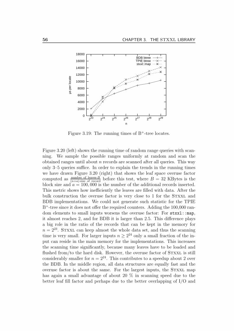
56 CHAPTER 3. THE STXXL LIBRARY
0
2000
4000
6000
8000
10000
12000
14000
16000
18000
229228227226225224223
µs p
er lo
cate
n
BDB btreeTPIE btreestxxl::map
Figure 3.19: The running times of B+-tree locates.
Figure 3.20 (left) shows the running time of random range queries with scan-ning. We sample the possible ranges uniformly at random and scan theobtained ranges until about n records are scanned after all queries. This wayonly 3–5 queries suffice. In order to explain the trends in the running timeswe have drawn Figure 3.20 (right) that shows the leaf space overuse factorcomputed as number of leaves·B
(n+a)·size of recordbefore this test, where B = 32 KBytes is the
block size and a = 100, 000 is the number of the additional records inserted.This metric shows how inefficiently the leaves are filled with data. After thebulk construction the overuse factor is very close to 1 for the Stxxl andBDB implementations. We could not generate such statistic for the TPIEB+-tree since it does not offer the required counters. Adding the 100,000 ran-dom elements to small inputs worsens the overuse factor: For stxxl::map,it almost reaches 2, and for BDB it is larger than 2.5. This difference playsa big role in the ratio of the records that can be kept in the memory forn = 223. Stxxl can keep almost the whole data set, and thus the scanningtime is very small. For larger inputs n ≥ 224 only a small fraction of the in-put can reside in the main memory for the implementations. This increasesthe scanning time significantly, because many leaves have to be loaded andflushed from/to the hard disk. However, the overuse factor of Stxxl is stillconsiderably smaller for n = 224. This contributes to a speedup about 2 overthe BDB. In the middle region, all data structures are equally fast and theoveruse factor is about the same. For the largest inputs, the Stxxl maphas again a small advantage of about 20 % in scanning speed due to thebetter leaf fill factor and perhaps due to the better overlapping of I/O and
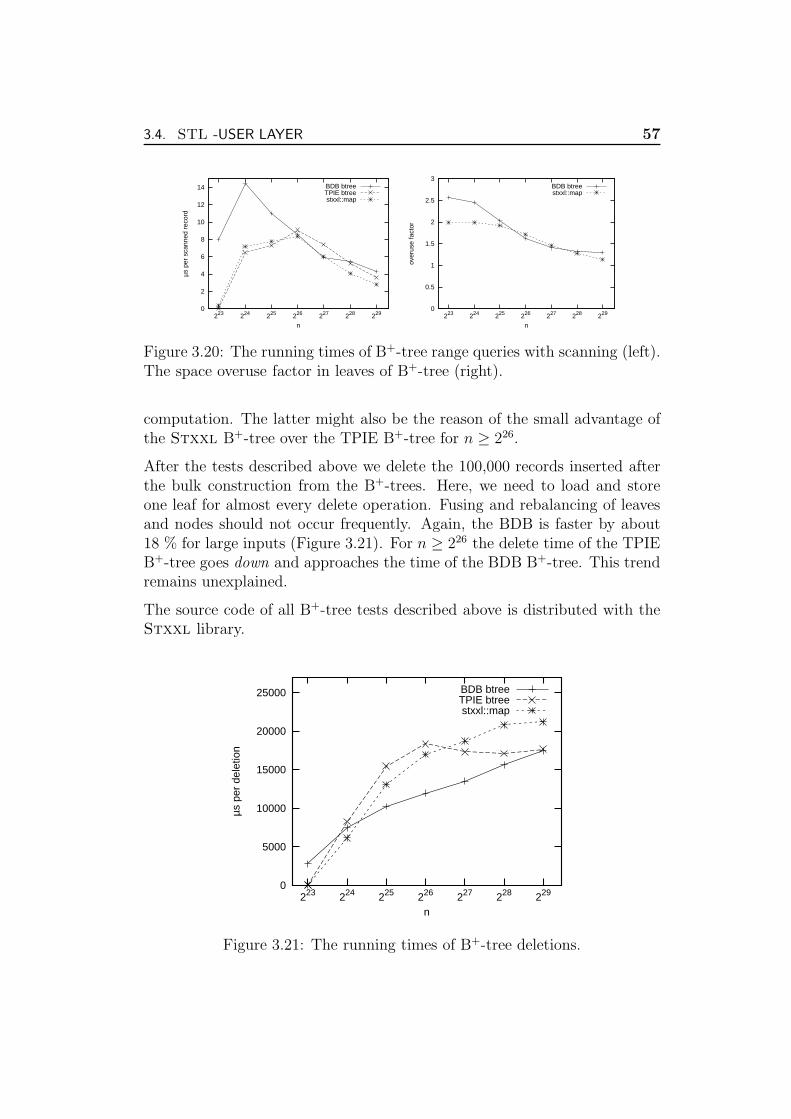
3.4. STL -USER LAYER 57
0
2
4
6
8
10
12
14
229228227226225224223
µs p
er s
cann
ed r
ecor
d
n
BDB btreeTPIE btreestxxl::map
0
0.5
1
1.5
2
2.5
3
229228227226225224223
over
use
fact
or
n
BDB btreestxxl::map
Figure 3.20: The running times of B+-tree range queries with scanning (left).The space overuse factor in leaves of B+-tree (right).
computation. The latter might also be the reason of the small advantage ofthe Stxxl B+-tree over the TPIE B+-tree for n ≥ 226.
After the tests described above we delete the 100,000 records inserted afterthe bulk construction from the B+-trees. Here, we need to load and storeone leaf for almost every delete operation. Fusing and rebalancing of leavesand nodes should not occur frequently. Again, the BDB is faster by about18 % for large inputs (Figure 3.21). For n ≥ 226 the delete time of the TPIEB+-tree goes down and approaches the time of the BDB B+-tree. This trendremains unexplained.
The source code of all B+-tree tests described above is distributed with theStxxl library.
0
5000
10000
15000
20000
25000
229228227226225224223
µs p
er d
elet
ion
n
BDB btreeTPIE btreestxxl::map
Figure 3.21: The running times of B+-tree deletions.
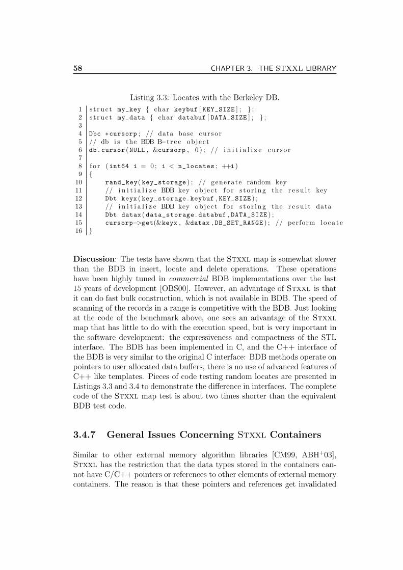
58 CHAPTER 3. THE STXXL LIBRARY
Listing 3.3: Locates with the Berkeley DB.
1 s t r u c t my_key char keybuf [ KEY_SIZE ] ; ;2 s t r u c t my_data char databuf [ DATA_SIZE ] ; ;34 Dbc ∗cursorp ; // data base cur so r5 // db i s the BDB B−t r e e ob j e c t6 db . cursor (NULL , &cursorp , 0 ) ; // i n i t i a l i z e cur so r78 f o r ( int64 i = 0 ; i < n_locates ; ++i )9
10 rand_key( key_storage ) ; // generate random key11 // i n i t i a l i z e BDB key ob je c t f o r s t o r i n g the r e s u l t key12 Dbt keyx ( key_storage . keybuf , KEY_SIZE ) ;13 // i n i t i a l i z e BDB key ob je c t f o r s t o r i n g the r e s u l t data14 Dbt datax ( data_storage . databuf , DATA_SIZE ) ;15 cursorp−>get(&keyx , &datax , DB_SET_RANGE ) ; // perform l o c a t e16
Discussion: The tests have shown that the Stxxl map is somewhat slowerthan the BDB in insert, locate and delete operations. These operationshave been highly tuned in commercial BDB implementations over the last15 years of development [OBS00]. However, an advantage of Stxxl is thatit can do fast bulk construction, which is not available in BDB. The speed ofscanning of the records in a range is competitive with the BDB. Just lookingat the code of the benchmark above, one sees an advantage of the Stxxl
map that has little to do with the execution speed, but is very important inthe software development: the expressiveness and compactness of the STLinterface. The BDB has been implemented in C, and the C++ interface ofthe BDB is very similar to the original C interface: BDB methods operate onpointers to user allocated data buffers, there is no use of advanced features ofC++ like templates. Pieces of code testing random locates are presented inListings 3.3 and 3.4 to demonstrate the difference in interfaces. The completecode of the Stxxl map test is about two times shorter than the equivalentBDB test code.
3.4.7 General Issues Concerning Stxxl Containers
Similar to other external memory algorithm libraries [CM99, ABH+03],Stxxl has the restriction that the data types stored in the containers can-not have C/C++ pointers or references to other elements of external memorycontainers. The reason is that these pointers and references get invalidated
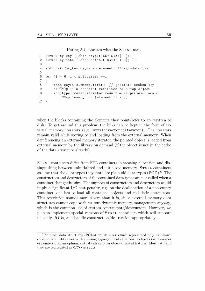
3.4. STL -USER LAYER 59
Listing 3.4: Locates with the Stxxl map.
1 s t r u c t my_key char keybuf [ KEY_SIZE ] ; ;2 s t r u c t my_data char databuf [ DATA_SIZE ] ; ;34 std : : pair<my_key , my_data> element ; // key−data pa i r56 f o r (i = 0 ; i < n_locates ; ++i )7 8 rand_key(i , element . first ) ; // generate random key9 // CMap i s a constant r e f e r e n c e to a map ob je c t
10 map_type : : const_iterator result = // perform l o c a t e11 CMap . lower_bound( element . first ) ;12
when the blocks containing the elements they point/refer to are written todisk. To get around this problem, the links can be kept in the form of ex-ternal memory iterators (e.g. stxxl::vector::iterator). The iteratorsremain valid while storing to and loading from the external memory. Whendereferencing an external memory iterator, the pointed object is loaded fromexternal memory by the library on demand (if the object is not in the cacheof the data structure already).
Stxxl containers differ from STL containers in treating allocation and dis-tinguishing between uninitialized and initialized memory. Stxxl containersassume that the data types they store are plain old data types (POD) 6. Theconstructors and destructors of the contained data types are not called when acontainer changes its size. The support of constructors and destructors wouldimply a significant I/O cost penalty, e.g. on the deallocation of a non-emptycontainer, one has to load all contained objects and call their destructors.This restriction sounds more severe than it is, since external memory datastructures cannot cope with custom dynamic memory management anyway,which is the common use of custom constructors/destructors. However, weplan to implement special versions of Stxxl containers which will supportnot only PODs, and handle construction/destruction appropriately.
6Plain old data structures (PODs) are data structures represented only as passivecollections of field values, without using aggregation of variable-size objects (as referencesor pointers), polymorphism, virtual calls or other object-oriented features. Most naturallythey are represented as C/C++ structs.

60 CHAPTER 3. THE STXXL LIBRARY
3.4.8 Algorithms
The algorithms of the STL can be divided into two groups by their memoryaccess pattern: scanning algorithms and random access algorithms.
Scanning Algorithms
Scanning algorithms work with Input, Output, Forward, and Bidirectional it-erators only. Since random access operations are not allowed with these kindsof iterators, the algorithms inherently exhibit a strong spatial locality of ref-erence. efficient. Stxxl containers and their iterators are STL-compatible,therefore one can directly apply STL scanning algorithms to them, and theywill run I/O-efficiently (see the use of std::generate and std::unique al-gorithms in the Listing 3.6). Scanning algorithms are the majority of theSTL algorithms (62 out of 71). Stxxl also offers specialized implemen-tations of some scanning algorithms (stxxl::for each, stxxl::generate,etc.), which perform better in terms of constant factors in the I/O volumeand internal CPU work. These implementations benefit from accessing lowerlevel interfaces of the BM layer instead of using iterator interfaces, resultingin a smaller CPU overhead. Being aware of the sequential access pattern ofthe applied algorithm, the Stxxl implementations can do prefetching anduse queued writing, thereby leading to the overlapping of I/O with compu-tation.
Random Access Algorithms
Random access algorithms require random access iterators, hence may per-form (many) random I/Os 7. For such algorithms, Stxxl provides special-ized I/O efficient implementations that work with STL-user layer externalmemory containers. Currently, the library provides two implementations ofsorting: an std::sort-like sorting routine – stxxl::sort, and a sorter thatexploits integer keys – stxxl::ksort. Both sorters are implementations ofparallel disk algorithms described in Section 3.5.
Listing 3.6 shows how to program using the STL-user layer and how Stxxl
containers can be used together with both Stxxl algorithms and STL algo-rithms. The definitions of the classes edge, random edge and edge cmp arein Listing 3.5. The purpose of our example is to generate a huge random
7 The std::nth element algorithm is an exception. It needs O(scan(n)) I/Os onaverage.

3.4. STL -USER LAYER 61
Listing 3.5: Definitions of classes.
1 s t r u c t edge // edge c l a s s2 i n t src , dst ; // nodes3 edge ( ) 4 edge ( i n t src_ , i n t dst_ ) : src ( src_ ) , dst ( dst_ ) 5 bool operator == ( const edge & b ) const 6 return src == b . src && dst == b . dst ;7 8 ;9 s t r u c t random_edge // random edge gene ra to r func to r
10 edge operator ( ) ( ) const 11 edge Edge ( random ()−1 ,random () −1);12 whi l e (Edge . dst == Edge . src )13 Edge . dst = random ( ) − 1 ; //no s e l f −l o ops14 return Edge ;15 16 ;17 s t r u c t edge_cmp // edge comparison func to r18 edge min_value ( ) const 19 return edge ( std : : numeric_limits<int > : :min ( ) , 0 ) ; ;20 edge max_value ( ) const 21 return edge ( std : : numeric_limits<int > : :max ( ) , 0 ) ; ;22 bool operator ( ) ( const edge & a ,23 const edge & b ) const 24 return a . src < b . src | |25 (a . src == b . src && a . dst < b . dst ) ;26 27 ;
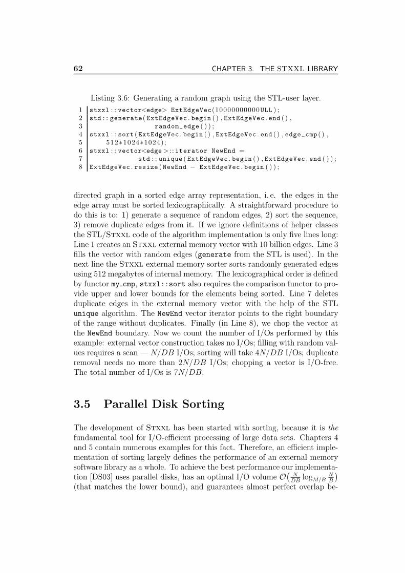
62 CHAPTER 3. THE STXXL LIBRARY
Listing 3.6: Generating a random graph using the STL-user layer.
1 stxxl : : vector<edge> ExtEdgeVec(10000000000ULL ) ;2 std : : generate( ExtEdgeVec . begin ( ) , ExtEdgeVec . end ( ) ,3 random_edge ( ) ) ;4 stxxl : : sort ( ExtEdgeVec . begin ( ) , ExtEdgeVec . end ( ) , edge_cmp ( ) ,5 512∗1024∗1024) ;6 stxxl : : vector<edge> : : iterator NewEnd =7 std : : unique ( ExtEdgeVec . begin ( ) , ExtEdgeVec . end ( ) ) ;8 ExtEdgeVec . resize ( NewEnd − ExtEdgeVec . begin ( ) ) ;
directed graph in a sorted edge array representation, i. e. the edges in theedge array must be sorted lexicographically. A straightforward procedure todo this is to: 1) generate a sequence of random edges, 2) sort the sequence,3) remove duplicate edges from it. If we ignore definitions of helper classesthe STL/Stxxl code of the algorithm implementation is only five lines long:Line 1 creates an Stxxl external memory vector with 10 billion edges. Line 3fills the vector with random edges (generate from the STL is used). In thenext line the Stxxl external memory sorter sorts randomly generated edgesusing 512 megabytes of internal memory. The lexicographical order is definedby functor my cmp, stxxl::sort also requires the comparison functor to pro-vide upper and lower bounds for the elements being sorted. Line 7 deletesduplicate edges in the external memory vector with the help of the STLunique algorithm. The NewEnd vector iterator points to the right boundaryof the range without duplicates. Finally (in Line 8), we chop the vector atthe NewEnd boundary. Now we count the number of I/Os performed by thisexample: external vector construction takes no I/Os; filling with random val-ues requires a scan — N/DB I/Os; sorting will take 4N/DB I/Os; duplicateremoval needs no more than 2N/DB I/Os; chopping a vector is I/O-free.The total number of I/Os is 7N/DB.
3.5 Parallel Disk Sorting
The development of Stxxl has been started with sorting, because it is thefundamental tool for I/O-efficient processing of large data sets. Chapters 4and 5 contain numerous examples for this fact. Therefore, an efficient imple-mentation of sorting largely defines the performance of an external memorysoftware library as a whole. To achieve the best performance our implementa-tion [DS03] uses parallel disks, has an optimal I/O volume O
(
NDB
logM/BNB
)
(that matches the lower bound), and guarantees almost perfect overlap be-
3.5. PARALLEL DISK SORTING 63
tween I/O and computation.
No previous implementation has all these properties, which are needed for agood practical sorting. LEDA-SM [CM99] and TPIE [APV02] concentrateon single disk implementations. For the overlapping of I/O and computationthey rely on prefetching and caching provided by the operating system, whichis suboptimal since the system knows little about the application’s accesspattern.
Barve and Vitter implemented a parallel disk algorithm [BGV97] that can beviewed as the immediate ancestor of our algorithm. Innovations with respectto our sorting are: A different allocation strategy that enables better theoret-ical I/O bounds [HSV01, KV01]; a prefetching algorithm that optimizes thenumber of I/O steps and never evicts data previously fetched; overlapping ofI/O and computation; a completely asynchronous implementation that re-acts flexibly to fluctuations in disk speeds; and an implementation that sortsmany GBytes and does not have to limit internal memory size artificially toobtain a nontrivial number of runs. Additionally, our implementation is nota prototype, it has a generic interface and is a part of the software libraryStxxl.
Algorithms in [Raj98, CC02, CCW01] have the theoretical advantage of beingdeterministic. However, they need three passes over data even for not toolarge inputs.
Prefetch buffers for disk load balancing and overlapping of I/O and com-putation have been intensively studied for external memory merge sort[PV92, CFKL96, AGL98, HSV01, KV01, KK00]. But we have not seen re-sults that guarantee overlapping of I/O and computation during the paralleldisk merging of arbitrary runs.
There are many good practical implementations of sorting (e.g. [NBC+94,Aga96, NKG00, Wyl99]) that address parallel disks, overlapping of I/O andcomputation, and have a low internal overhead. However, we are not aware offast implementations that give theoretical performance guarantees on achiev-ing asymptotically optimal I/O. Most practical implementations use a formof striping that requires Ω( N
DBlogΘ( M
DB)
NB
) I/Os rather than the optimal
Θ( NDB
logΘ(M/B)NB
). This difference is usually considered insignificant forpractical purposes. However, already on our experimental system we haveto go somewhat below the block sizes that give the best performance in Fig-ure 3.31 if the input size is 128 GBytes. Another reduction of the block sizeby a factor of eight (we have eight disks) could increase the run time sig-nificantly. We are also not aware of high performance implementations that
64 CHAPTER 3. THE STXXL LIBRARY
guarantee overlap of I/O and computation during merging for inputs such asthe one described in Section 3.5.1.
On the other hand, many of the practical merits of our implementation areat least comparable with the best current implementations: We are close tothe peak performance of our system.
The Sort Benchmark competition [Gra] is held yearly and includes severalcategories; some of them define restrictions on the cost of the hardware usedfor sorting. In the “Terabyte” category, the goal is to sort quickly a terabyteof data. As this benchmark type is not limited by the hardware costs, dis-tributed memory sorting algorithms running on expensive clusters with SANdisks win. Distributed memory sorters also lead in the “Minute” categorywhich asks to sort as much data as possible in a minute. In the “Penny” cate-gory the cost of the hardware is spread over three years. Then, it is measuredhow much data can be sorted in an interval of time that costs one US-cent.Competition participants are responsible for the choice of their hardware.Each category has two subcategories: Daytona (for general-purpose sorting)and Indy (sort 100-byte records with 10-byte random keys).
The most interesting category for us is the “Penny” category because it ad-dresses the cost-efficiency aspect of sorting, and it turns out that the cheapestway to sort is to use an I/O-efficient sorting. All winners in this categorysince the announcement in 1998 were external memory sorters. We overviewthe past “Penny sort” winners [Gra]. The NTSort (won Indy in 1998) is acommand line sorting utility of Windows NT implementing multi-way mergesort. The implementation adopted for the competition relied on direct un-buffered I/O, but used no overlapping between I/O and computation. Post-manSort (Daytona winner in 1998 and 2005) is a commercial sorting utility;it is a variant of the bucket sort. The recent version utilizes asynchronousI/O of Windows to overlap I/O and computation. HMSort (winner in 1999and 2000) also exploits overlapping of I/O and computation, however, otherdetails about the algorithm are not published. DMSort (Indy 2002) is basedon the most-significant byte radix sort. The implementation works with twodisks: The input data elements are read from the first disk and distributedto the bins on the second disk, explicitly overlapping I/O and computa-tion. The second phase reads the bins from the second disk, sorts them, andwrites the sorted result to the first disk in an overlapped fashion. Only fewalgorithmic details of THSort (Daytona 2004), Sheenksort (Indy 2004, 2005)and Byte-Split-Index Sort (Daytona 2006) are published. The authors ofthe THSort, SheenkSort and Byte-Split-Index have used systems with fourdisks. The GpuTeraSort (Indy 2006) [GGKM05] uses a graphic processingunit (GPU) for internal sorting, mapping a bitonic sorting network to GPU
3.5. PARALLEL DISK SORTING 65
rasterization operations and using the GPUs programmable hardware andhigh bandwidth memory interface. The implementation accesses the filesdirectly and explictly overlaps I/O and computation. To achieve a higherI/O-bandwidth, a RAID-0 has been used.
We have participated in the “Penny” sort competition in 2003 with an earliervariant of the implementation presented below. We took the second place,sorting 25 GBytes in our time budget. We would have been be very close tothe winner’s value of 40 GBytes if we had been more lucky with the choice ofhardware: Our more expensive system ran with errors at the full speed, wealso have overlooked the fast (and cheap) hard disks used by our opponents,because the manufacturer did not bother to specify their characteristics. The“Penny sort” external sorters mentioned above are very impressive pieces ofengineering. However, these algorithms and implementations do not givetheoretical guarantees of the performance, including the overlapping of I/Oand computation and the optimal use of parallel disks.
3.5.1 Multi-way Merge Sort with Overlapped I/Os
Perhaps the most widely used external memory sorting algorithm is k-waymerge sort: During run formation, chunks of Θ(M) elements are read, sortedinternally, and written back to the disk as sorted runs. The runs are thenmerged into larger runs until only a single run is left. k = O(M/B) runscan be sorted in a single pass by keeping up to B of the smallest elements ofeach run in internal memory. Using randomization, prediction of the order inwhich blocks are accessed, a prefetch buffer of O(D) blocks, and an optimalprefetching strategy, it is possible to implement k-way merging using D disksin a load balanced way [HSV01]. However, the rate at which new blocks arerequested is more difficult to predict so that this algorithm does not guaranteeoverlapping of I/O and computation. In this section, we derive a parallel diskalgorithm that compensates these fluctuations in the block request rate by aFIFO buffer of k + Θ(D) blocks.
Run Formation
There are many ways to overlap I/O and run formation. We start with avery simple method that treats internal sorting as a black box and thereforecan use the fastest available internal sorters. Two threads cooperate to buildk runs of size M/2:

66 CHAPTER 3. THE STXXL LIBRARY
post a read request for runs 1 and 2
thread A: | thread B:
for r:=1 to k do | for r:=1 to k-2 do
wait until | wait until
run r is read | run r is written
sort run r | post a read for run r+2
post a write for run r |
Figure 3.22 illustrates how I/O and computation is overlapped by this al-gorithm. Formalizing this figure, we can prove that using this approach aninput of size N can be transformed into sorted runs of size M/2−O(DB) intime max(2Tsort(M/2)N/M, 2LN
DB) +O
(
LMDB
)
, where Tsort(x) denotes the timefor sorting x elements internally and where L is the time needed for a parallelI/O step.
In [DS03] one can find an algorithm which generates longer runs of averagelength 2M and overlaps I/O and computation.
Multi-way Merging
We want to merge k sorted sequences comprising N ′ elements stored in N ′/Bblocks (In practical situations, where a single merging phase suffices, we willhave N ′ = N). In each iteration, the merging thread chooses the smallestremaining element from the k sequences and hands it over to the I/O thread.Prediction of read operations is based on the observation that the mergingthread does not need to access a block until its smallest element becomes
sort
read
write
1 2
2
2
1
1
3
3
3
4
4
4
k−1
k−1
k−1
k
k
k
...
...
...
computebound case
I/Obound case
time
control flow in thread A
sort
read
write
1
1
1
2
2
3
2
3
3
4
4
4
...
...
...
k−1
k−1
k−1
k
k
k
control flow in thread B
Figure 3.22: Overlapping I/O and computation during run formation.

3.5. PARALLEL DISK SORTING 67
the smallest unread element. We therefore record the smallest keys of eachblock during run formation. By merging the resulting k sequences of smallestelements, we can produce a sequence σ of block identifiers that indicates theexact order in which blocks are logically read by the merging thread. Theoverhead for producing and storing the prediction data structure is negligiblebecause its size is a factor at least B smaller than the input.
The prediction sequence σ is used as follows. The merging thread maintainsthe invariant that it always buffers the k first blocks in σ that contain uns-elected elements, i.e., initially, the first k blocks from σ are read into thesemerge buffers. When the last element of a merge buffer block is selected, thenow empty buffer frame is returned to the I/O thread and the next block inσ is read.
The keys of the smallest elements in each buffer block are kept in a tourna-ment tree data structure [Knu98] so that the currently smallest element canbe selected in time O(log k). Hence, the total internal work for merging isO(N ′ log k).
We have now defined multi-way merging from the point of view of the sort-ing algorithm. Our approach to merging slightly deviates from previousapproaches that keep track of the run numbers of the merge blocks andpre-assign each merge block to the corresponding input sequence. In theseapproaches also the last key in the previous block decides about the positionof a block in σ. The correctness of our approach is shown in [DS03]. Withrespect to performance, both approaches should be similar. Our approach issomewhat simpler, however — note that the merging thread does not needto know anything about the k input runs and how they are allocated. Itsonly input is the prediction sequence σ. In a sense, we are merging individualblocks and the order in σ makes sure that the overall effect is that the inputruns are merged. A conceptual advantage is that data within a block decidesabout when a block is read.
Overlapping I/O and Merging
Although we can predict the order in which blocks are read, we cannot easilypredict how much internal work is done between two reads. For example,consider k identical runs storing the sequence 1B−12 3B−14 5B−16 · · · . Afterinitializing the merge buffers, the merging thread will consume k(B−1) values‘1’ before it posts another read. Then it will post one read after selecting eachof the next k values (2). Then there will be a pause of another k(B−1) stepsand another k reads are following each other quickly, etc. We explain how to
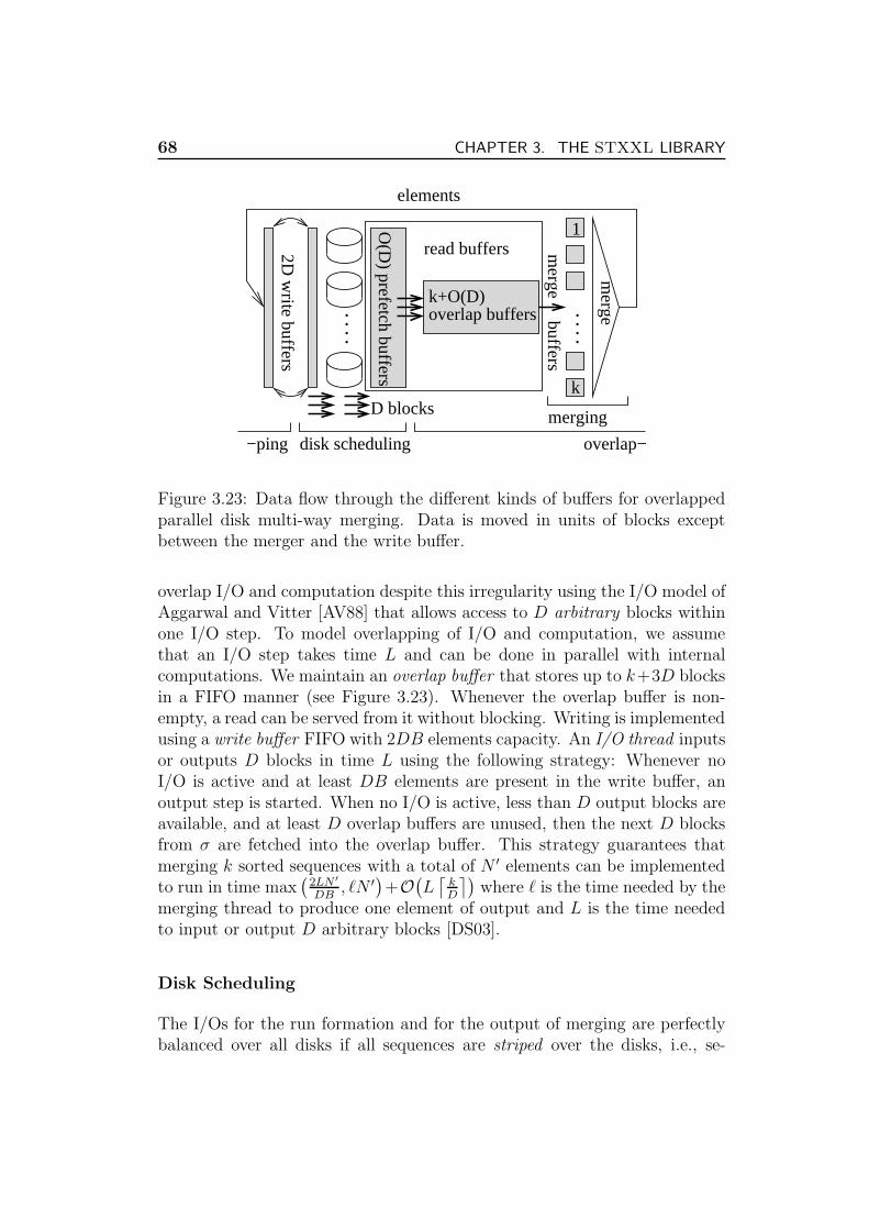
68 CHAPTER 3. THE STXXL LIBRARY
.
.
..
read buffers
.
.
..
k+O(D)overlap buffers
merging
−ping disk scheduling
1
k
merge
2D w
rite buffers
D blocks
merge buffers
overlap−
elements
O(D
) prefetch buffersFigure 3.23: Data flow through the different kinds of buffers for overlappedparallel disk multi-way merging. Data is moved in units of blocks exceptbetween the merger and the write buffer.
overlap I/O and computation despite this irregularity using the I/O model ofAggarwal and Vitter [AV88] that allows access to D arbitrary blocks withinone I/O step. To model overlapping of I/O and computation, we assumethat an I/O step takes time L and can be done in parallel with internalcomputations. We maintain an overlap buffer that stores up to k+3D blocksin a FIFO manner (see Figure 3.23). Whenever the overlap buffer is non-empty, a read can be served from it without blocking. Writing is implementedusing a write buffer FIFO with 2DB elements capacity. An I/O thread inputsor outputs D blocks in time L using the following strategy: Whenever noI/O is active and at least DB elements are present in the write buffer, anoutput step is started. When no I/O is active, less than D output blocks areavailable, and at least D overlap buffers are unused, then the next D blocksfrom σ are fetched into the overlap buffer. This strategy guarantees thatmerging k sorted sequences with a total of N ′ elements can be implementedto run in time max
(
2LN ′
DB, ℓN ′
)
+O(
L⌈
kD
⌉)
where ℓ is the time needed by themerging thread to produce one element of output and L is the time neededto input or output D arbitrary blocks [DS03].
Disk Scheduling
The I/Os for the run formation and for the output of merging are perfectlybalanced over all disks if all sequences are striped over the disks, i.e., se-
3.5. PARALLEL DISK SORTING 69
quences are stored in blocks of B elements each and the blocks numberedi,. . . ,i + D − 1 in a sequence are stored on different disks for all i. In partic-ular, the original input and the final output of sorting can use any kind ofstriping.
The merging algorithm presented above is optimal for the unrealistic modelof Aggarwal and Vitter [AV88] which allows to access any D blocks in an I/Ostep. This facilitates good performance for fetching very irregularly placedinput blocks. However, this model can be simulated using D independentdisks using randomized striping allocation [VH01] and a prefetch buffer ofsize m = Θ(D) blocks: In almost every input step, (1 − O(D/m))D blocksfrom prefetch sequence σ can be fetched [DS03].
Figure 3.23 illustrates the data flow between the components of our paralleldisk multi-way merging.
3.5.2 Implementation Details
Run Formation. We build runs of a size close to M/2 but there aresome differences to the simple algorithm from Section 3.5.1. Overlapping ofI/O and computation is achieved using the call-back mechanism supportedby the I/O layer. Thus, the sorter remains portable over different operatingsystems with different interfaces to threading.
We have two implementations with respect to the internal work:stxxl::sort is a comparison based sorting using std::sort from STL tosort the runs internally; stxxl::ksort exploits integer keys and has smallerinternal memory bandwidth requirements for large elements with small keyfields. After reading elements using DMA (i.e. the Stxxl direct access), weextract pairs (key, pointerToElement), sort these pairs, and only then moveelements in sorted order to write buffers from where they are output usingDMA.
Furthermore, we exploit random keys. We use two passes of MSD (mostsignificant digit) radix sort of the key-pointer pairs. The first pass uses them most significant bits where m is a tuning parameter depending on thesize of the processor caches and of the TLB (translation look-aside buffer).This pass consists of a counting phase that determines bucket sizes and adistribution phase that moves pairs. The counting phase is fused into a singleloop with pair extraction. The second pass of radix sort uses a number ofbits that brings us closest to an expected bucket size of two. This two-pass
70 CHAPTER 3. THE STXXL LIBRARY
algorithm is much more cache efficient than a one-pass radix sort.8 Theremaining buckets are sorted using a comparison based algorithm: Optimalstraight line code for n ≤ 4, insertion sort for n ∈ 5..16, and quicksort forn > 16.
Multi-way Merging. We have adapted the tuned multi-way merger from[San00], i.e. a tournament tree stores pointers to the current elements of eachmerge buffer.
Overlapping I/O and Computation. We integrate the prefetch bufferand the overlap buffer to a read buffer. We distribute the buffer space be-tween the two purposes of minimizing disk idle time and overlapping I/Oand computation indirectly by computing an optimal prefetch sequence fora smaller buffer space.
Asynchronous I/O. I/O is performed without any synchronization be-tween the disks. The prefetcher computes a sequence σ′ of blocks indicatingthe order in which blocks should be fetched. As soon as a buffer block be-comes available for prefetching, it is used to generate an asynchronous readrequest for the next block in σ′. The I/O layer of Stxxl queues this re-quest at the disk storing the block to be fetched. The thread for this diskserves the queued request in FIFO manner. All I/O is implemented withoutsuperfluous copying. Stxxl opens files with the option O DIRECT so thatblocks are directly moved by DMA (direct memory access) to user memory.A fetched block then travels to the prefetch/overlap buffer and from thereto a merge buffer simply by passing a pointer. Similarly, when an elementis merged, it is directly moved from the merge buffer to the write buffer anda block of the write buffer is passed to the output queue of a disk simplyby passing a pointer to the the I/O layer of Stxxl that then uses write tooutput the data using DMA.
3.5.3 Experiments
Hardware. For the experiments we have used the system with two 2GHzXeon processors, one GByte of RAM and eight IDE disks (described in Sec-tion 2.4). The maximum parallel disk bandwidth from the outermost (fastest)zones was about 375 MB/s.
8On our system we get a factor of 3.8 speedup over the one pass radix sort and a factorof 1.6 over STL’s sort which in turn is faster than a hand tuned quicksort (for sorting 221
pairs storing a random four byte key and a pointer).
3.5. PARALLEL DISK SORTING 71
Software. The system ran the Debian Linux distribution with kernel 2.4.20and the ext2 file system. All programs were compiled with g++ version 3.2and the optimization level -O3.
If not otherwise mentioned, we use random 32 bit integer keys to keep internalwork limited. Runs of size 256 MByte9 are built using key sorting with aninitial iteration of 10 bit MSD radix sort. We choose block sizes in such a waythat a single merging phase using 512 MBytes for all buffers suffices. Inputsizes are powers of two between 2 GByte and 128 GByte with a default of 16GByte10. When not otherwise stated, we use eight disks, 2 MByte blocks,and the input is stored on the fastest zones.
To compare our code with previous implementations, we have to run themon the same machine because technological development in recent years hasbeen very fast. Unfortunately, the implementations we could obtain, LEDA-SM [CM00] and TPIE [vdBDS00], are limited to inputs of size 2 GBytewhich, for our machine, is a rather small input. Figure 3.24 compares thesingle disk performance of the three libraries using the best block size foreach library. The flat curves for TPIE and Stxxl indicate that both codesare I/O bound even for small element sizes. This is even true for the fullycomparison based version of Stxxl. Still, Stxxl is significantly faster thanTPIE. This could be due to better overlapping of I/O and computation ordue to the higher bandwidth of the file system calls we use. Stxxl sustainsan I/O bandwidth of 45.4 MByte/s, which is 95 % of the 48 MByte/s peakbandwidth of the disk at their outermost zone. LEDA-SM is compute-boundfor small keys and has the same performance as TPIE for large keys.
To get some kind of comparison for parallel disks, we ran the other codesusing Linux Software-RAID 0.9 and 8 × 128KBytes stripes (larger stripesdid not improve performance). Here, Stxxl is between two and three timesfaster than TPIE and sustains an I/O bandwidth of 315 MByte/s for largeelements. Much of this advantage is lost when Stxxl also runs on theSoftware-RAID. Although we view it as likely that the Software-RAID drivercan be improved, this performance difference might also be an indication thattreating disks as independent devices is better than striping (as predicted bytheory).
Figure 3.26 shows the dependence of the performance on the element size inmore detail. For element sizes ≥ 64, the merging phase starts to wait for I/Os
9This leaves space for two runs build in an overlapped way, buffers, operating system,code, and, for large inputs, the fact that the implementation of the ext2 file system needed1 byte of internal memory for each KBytes of disk space accessed via O DIRECT.
10We have a few measurements with 256 GBytes but the problem with ext2 mentionedabove starts to distort the results for this input size.
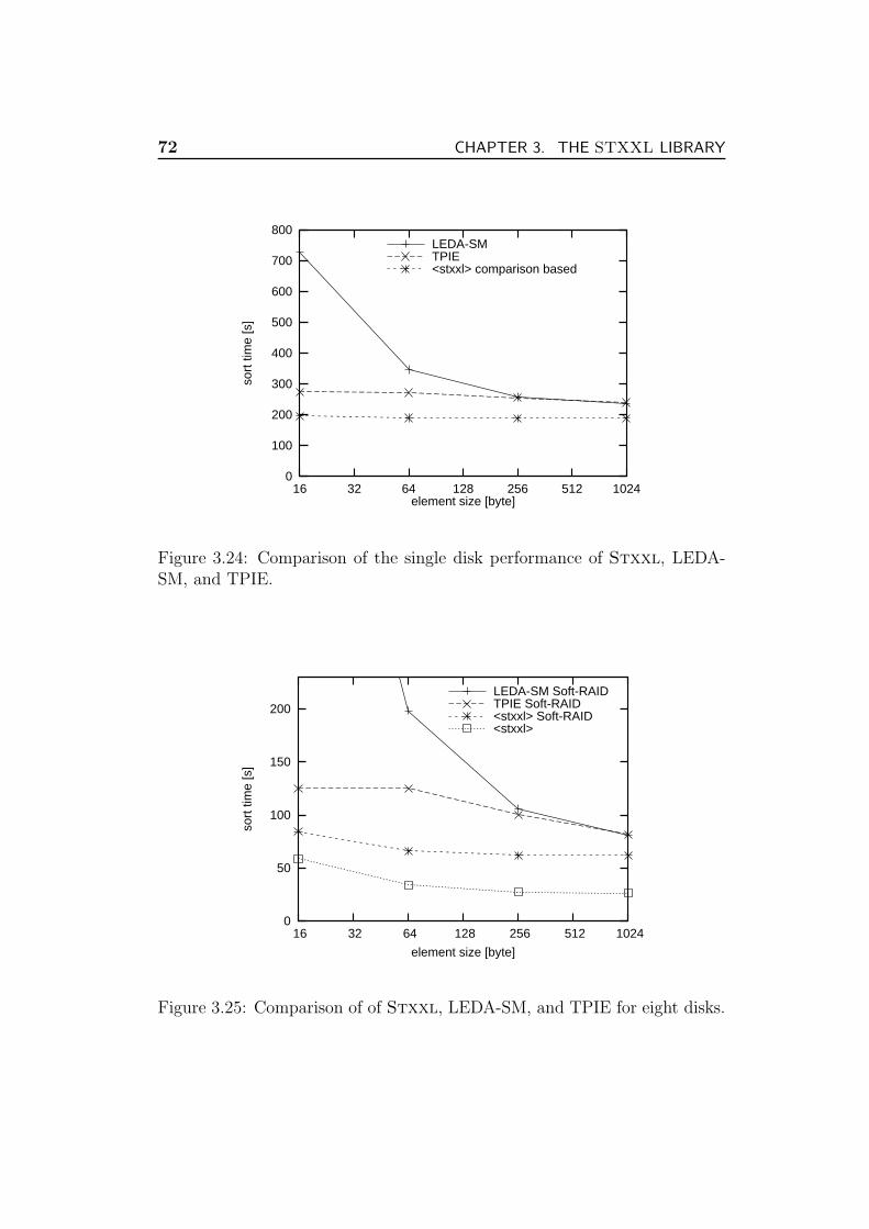
72 CHAPTER 3. THE STXXL LIBRARY
0
100
200
300
400
500
600
700
800
16 32 64 128 256 512 1024
sort
tim
e [s
]
element size [byte]
LEDA-SMTPIE<stxxl> comparison based
Figure 3.24: Comparison of the single disk performance of Stxxl, LEDA-SM, and TPIE.
0
50
100
150
200
16 32 64 128 256 512 1024
sort
tim
e [s
]
element size [byte]
LEDA-SM Soft-RAIDTPIE Soft-RAID<stxxl> Soft-RAID<stxxl>
Figure 3.25: Comparison of of Stxxl, LEDA-SM, and TPIE for eight disks.
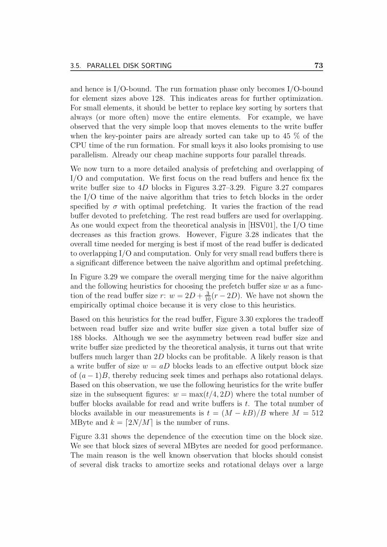
3.5. PARALLEL DISK SORTING 73
and hence is I/O-bound. The run formation phase only becomes I/O-boundfor element sizes above 128. This indicates areas for further optimization.For small elements, it should be better to replace key sorting by sorters thatalways (or more often) move the entire elements. For example, we haveobserved that the very simple loop that moves elements to the write bufferwhen the key-pointer pairs are already sorted can take up to 45 % of theCPU time of the run formation. For small keys it also looks promising to useparallelism. Already our cheap machine supports four parallel threads.
We now turn to a more detailed analysis of prefetching and overlapping ofI/O and computation. We first focus on the read buffers and hence fix thewrite buffer size to 4D blocks in Figures 3.27–3.29. Figure 3.27 comparesthe I/O time of the naive algorithm that tries to fetch blocks in the orderspecified by σ with optimal prefetching. It varies the fraction of the readbuffer devoted to prefetching. The rest read buffers are used for overlapping.As one would expect from the theoretical analysis in [HSV01], the I/O timedecreases as this fraction grows. However, Figure 3.28 indicates that theoverall time needed for merging is best if most of the read buffer is dedicatedto overlapping I/O and computation. Only for very small read buffers there isa significant difference between the naive algorithm and optimal prefetching.
In Figure 3.29 we compare the overall merging time for the naive algorithmand the following heuristics for choosing the prefetch buffer size w as a func-tion of the read buffer size r: w = 2D + 3
10(r − 2D). We have not shown the
empirically optimal choice because it is very close to this heuristics.
Based on this heuristics for the read buffer, Figure 3.30 explores the tradeoffbetween read buffer size and write buffer size given a total buffer size of188 blocks. Although we see the asymmetry between read buffer size andwrite buffer size predicted by the theoretical analysis, it turns out that writebuffers much larger than 2D blocks can be profitable. A likely reason is thata write buffer of size w = aD blocks leads to an effective output block sizeof (a− 1)B, thereby reducing seek times and perhaps also rotational delays.Based on this observation, we use the following heuristics for the write buffersize in the subsequent figures: w = max(t/4, 2D) where the total number ofbuffer blocks available for read and write buffers is t. The total number ofblocks available in our measurements is t = (M − kB)/B where M = 512MByte and k = ⌈2N/M⌉ is the number of runs.
Figure 3.31 shows the dependence of the execution time on the block size.We see that block sizes of several MBytes are needed for good performance.The main reason is the well known observation that blocks should consistof several disk tracks to amortize seeks and rotational delays over a large
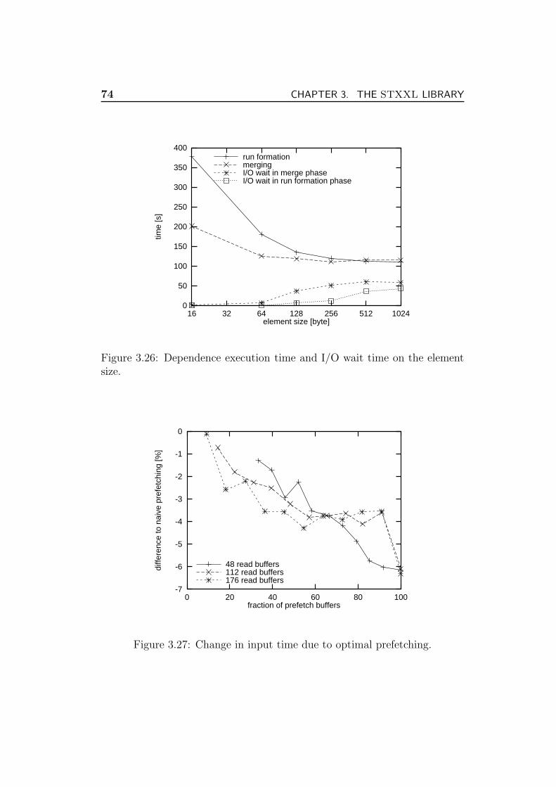
74 CHAPTER 3. THE STXXL LIBRARY
0
50
100
150
200
250
300
350
400
16 32 64 128 256 512 1024
time
[s]
element size [byte]
run formationmergingI/O wait in merge phaseI/O wait in run formation phase
Figure 3.26: Dependence execution time and I/O wait time on the elementsize.
-7
-6
-5
-4
-3
-2
-1
0
0 20 40 60 80 100
diffe
renc
e to
nai
ve p
refe
tchi
ng [%
]
fraction of prefetch buffers
48 read buffers112 read buffers176 read buffers
Figure 3.27: Change in input time due to optimal prefetching.
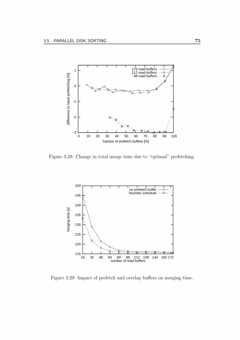
3.5. PARALLEL DISK SORTING 75
1
0
-1
-2
-3 0 10 20 30 40 50 60 70 80 90 100
diffe
renc
e to
nai
ve p
refe
tchi
ng [%
]
fraction of prefetch buffers [%]
176 read buffers112 read buffers48 read buffers
Figure 3.28: Change in total merge time due to “optimal” prefetching.
115
120
125
130
135
140
145
150
16 32 48 64 80 96 112 128 144 160 172
mer
ging
tim
e [s
]
number of read buffers
no prefetch bufferheuristic schedule
Figure 3.29: Impact of prefetch and overlap buffers on merging time.
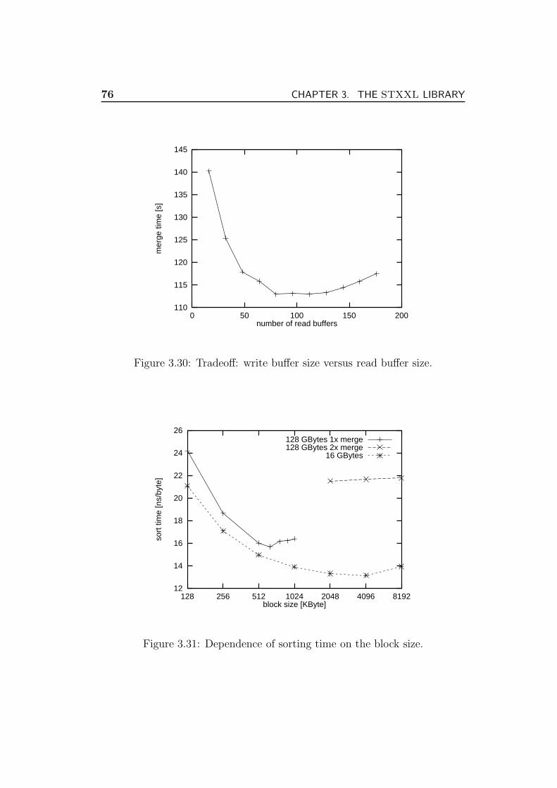
76 CHAPTER 3. THE STXXL LIBRARY
110
115
120
125
130
135
140
145
0 50 100 150 200
mer
ge ti
me
[s]
number of read buffers
Figure 3.30: Tradeoff: write buffer size versus read buffer size.
12
14
16
18
20
22
24
26
128 256 512 1024 2048 4096 8192
sort
tim
e [n
s/by
te]
block size [KByte]
128 GBytes 1x merge128 GBytes 2x merge
16 GBytes
Figure 3.31: Dependence of sorting time on the block size.
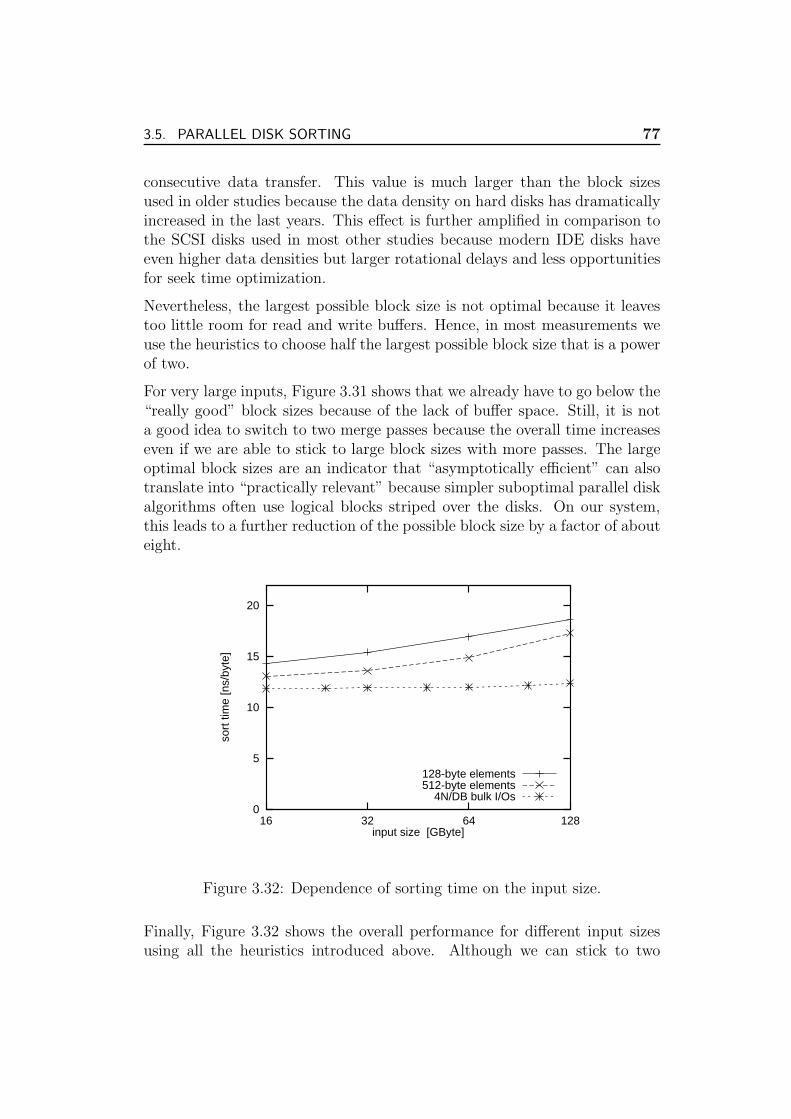
3.5. PARALLEL DISK SORTING 77
consecutive data transfer. This value is much larger than the block sizesused in older studies because the data density on hard disks has dramaticallyincreased in the last years. This effect is further amplified in comparison tothe SCSI disks used in most other studies because modern IDE disks haveeven higher data densities but larger rotational delays and less opportunitiesfor seek time optimization.
Nevertheless, the largest possible block size is not optimal because it leavestoo little room for read and write buffers. Hence, in most measurements weuse the heuristics to choose half the largest possible block size that is a powerof two.
For very large inputs, Figure 3.31 shows that we already have to go below the“really good” block sizes because of the lack of buffer space. Still, it is nota good idea to switch to two merge passes because the overall time increaseseven if we are able to stick to large block sizes with more passes. The largeoptimal block sizes are an indicator that “asymptotically efficient” can alsotranslate into “practically relevant” because simpler suboptimal parallel diskalgorithms often use logical blocks striped over the disks. On our system,this leads to a further reduction of the possible block size by a factor of abouteight.
0
5
10
15
20
16 32 64 128
sort
tim
e [n
s/by
te]
input size [GByte]
128-byte elements512-byte elements
4N/DB bulk I/Os
Figure 3.32: Dependence of sorting time on the input size.
Finally, Figure 3.32 shows the overall performance for different input sizesusing all the heuristics introduced above. Although we can stick to two
78 CHAPTER 3. THE STXXL LIBRARY
passes, the execution time per element goes up because we need to employincreasingly slow zones, because the block sizes go down, and because theseek times go during merging up.
3.5.4 Discussion
We have engineered a sorting algorithm that combines a very high perfor-mance on state of the art hardware with theoretical performance guarantees.This algorithm is compute-bound although we use small random keys and atuned linear time algorithm for the run formation. Similar observations ap-ply to other external memory algorithms that exhibit a good spatial locality,i.e. those dominated by scanning, sorting, and similar operations (see e.g.Chapters 4 and 5). This indicates that bandwidth is no longer a limitingfactor for external memory algorithms if parallel disks are used.
On the other hand, the fact that it is challenging to sustain a peak band-width for eight disks on a dual processor system implies that using even moredisks requires a more aggressive use of parallel processing. Using the MCSTL[Sin06] library we have parallelized the internal work in the run formationand merge phases of our implementation. On the SCSIOpteron system (Sec-tion 2.4) with eight fast SCSI disks we have sorted small 8-byte records witha speedup close to two using four processors. The compute bound could beraised by dividing the load onto many processors [Sin06].
Algorithmically, several promising improvements remain, even for smallcheap machines: There are several ways to speed up the run formation forsmall elements. During merging, it would be good to reduce seek times forlarge inputs, either by some clever compromise between seek minimizationand prefetching, or by switching to the distribution sort [VH01] that can beimplemented to have an inherently low seek overhead.
3.6. ALGORITHM PIPELINING 79
3.6 Algorithm Pipelining
The pipelined processing technique is very well known in the database world[SKS01].
Usually, the interface of an external memory algorithm assumes that it readsthe input from (an) external memory container(s) and writes output into(an) external memory container(s). The idea of pipelining is to equip theexternal memory algorithms with a new interface that allows them to feedthe output as a data stream directly to the algorithm that consumes theoutput, rather than writing it to the external memory first. Logically, theinput of an external memory algorithm does not have to reside in the externalmemory, rather, it could be a data stream produced by another externalmemory algorithm.
Many external memory algorithms can be viewed as a data flow througha directed acyclic graph G with node set V = F ∪ S ∪ R and edge setE. The file nodes F represent physical data sources and data sinks, whichare stored on disks (e.g. in the external memory containers of the STL-userlayer). A file node writes or/and reads one stream of elements. The streamingnodes S read zero, one or several streams and output zero, one or severalnew streams. Streaming nodes are equivalent to scan operations in non-pipelined external memory algorithms. The difference is that non-pipelinedconventional scanning needs a linear number of I/Os, whereas streamingnodes usually do not perform any I/O, unless a node needs to access externalmemory data structures (stacks, priority queues, etc.). The sorting nodes Rread a stream and output it in a sorted order. Edges E in the graph Gdenote the directions of data flow between nodes. The question “When is apipelined execution of the computations in a data flow graph G possible inan I/O-efficient way?” is analyzed in [DMKS05].
3.7 Streaming Layer
The streaming layer provides a framework for the pipelined processing of largesequences. Many external memory algorithms implemented with the Stxxl
streaming layer save a factor of at least two in I/Os. To the best of ourknowledge we are the first who apply the pipelining method systematicallyin the domain of external memory algorithms. We introduce it in the contextof an external memory software library.
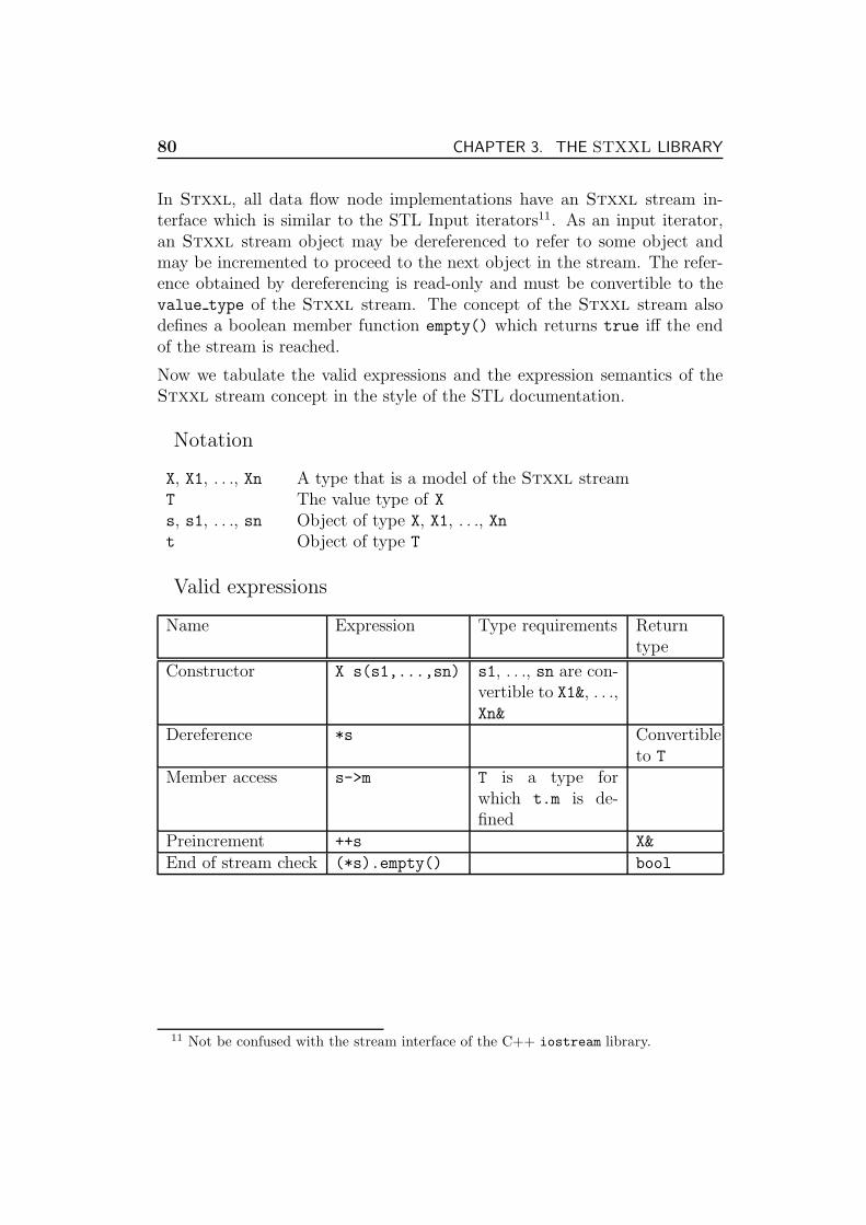
80 CHAPTER 3. THE STXXL LIBRARY
In Stxxl, all data flow node implementations have an Stxxl stream in-terface which is similar to the STL Input iterators11. As an input iterator,an Stxxl stream object may be dereferenced to refer to some object andmay be incremented to proceed to the next object in the stream. The refer-ence obtained by dereferencing is read-only and must be convertible to thevalue type of the Stxxl stream. The concept of the Stxxl stream alsodefines a boolean member function empty() which returns true iff the endof the stream is reached.
Now we tabulate the valid expressions and the expression semantics of theStxxl stream concept in the style of the STL documentation.
Notation
X, X1, . . ., Xn A type that is a model of the Stxxl streamT The value type of Xs, s1, . . ., sn Object of type X, X1, . . ., Xnt Object of type T
Valid expressions
Name Expression Type requirements Returntype
Constructor X s(s1,...,sn) s1, . . ., sn are con-vertible to X1&, . . .,Xn&
Dereference *s Convertibleto T
Member access s->m T is a type forwhich t.m is de-fined
Preincrement ++s X&
End of stream check (*s).empty() bool
11 Not be confused with the stream interface of the C++ iostream library.

3.7. STREAMING LAYER 81
Expression semantics
Name Expression Precondition Semantics Postcondition
Constructor X s(s1,...,sn) s1, . . .,sn are then inputstreams ofs
Dereference *s s is incre-mentable
Memberaccess
s->m s is incre-mentable
Equivalentto (*s).m
Preincrement ++s s is incre-mentable
s is incre-mentable orpast-the-end
The binding of a Stxxl stream object to its input streams (incoming edgesin a data flow graph G) happens at compile time, i.e. statically. The otherapproach would be to allow binding at running time using the C++ vir-tual function mechanism. However this would result in a severe perfor-mance penalty because most C++ compilers are not able to inline vir-tual functions. To avoid this disadvantage, we follow the static bindingapproach using C++ templates. For example, assuming that streams s1,. . ., sn are already constructed, construction of stream s with constructorX::X(X1& s1,..., Xn& sn) will bind s to its inputs s1, . . ., sn.
After creating all node objects, the computation starts in a “lazy” fashion,first trying to evaluate the result of the topologically latest node. The nodereads its intermediate input nodes, element by element, using the dereferenceand increment operator of the Stxxl stream interface. The input nodesproceed in the same way, invoking the inputs needed to produce an outputelement. This process terminates when the result of the topologically latestnode is computed. This style of pipelined execution scheduling is I/O effi-cient, it allows to keep the intermediate results in-memory without needingto store them in external memory.
The Streaming layer of the Stxxl library offers generic classes which imple-ment the functionality of sorting, file, and streaming nodes:
• File nodes: Function streamify serves as an adaptor that converts arange of ForwardIterators into a compatible Stxxl stream. Since it-erators of stxxl::vector are RandomAccessIterators, streamify can
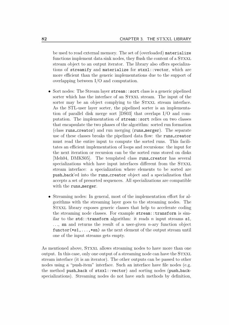
82 CHAPTER 3. THE STXXL LIBRARY
be used to read external memory. The set of (overloaded) materializefunctions implement data sink nodes, they flush the content of a Stxxl
stream object to an output iterator. The library also offers specializa-tions of streamify and materialize for stxxl::vector, which aremore efficient than the generic implementations due to the support ofoverlapping between I/O and computation.
• Sort nodes: The Stream layer stream::sort class is a generic pipelinedsorter which has the interface of an Stxxl stream. The input of thesorter may be an object complying to the Stxxl stream interface.As the STL-user layer sorter, the pipelined sorter is an implementa-tion of parallel disk merge sort [DS03] that overlaps I/O and com-putation. The implementation of stream::sort relies on two classesthat encapsulate the two phases of the algorithm: sorted run formation(class runs creator) and run merging (runs merger). The separateuse of these classes breaks the pipelined data flow: the runs creator
must read the entire input to compute the sorted runs. This facili-tates an efficient implementation of loops and recursions: the input forthe next iteration or recursion can be the sorted runs stored on disks[Meh04, DMKS05]. The templated class runs creator has severalspecializations which have input interfaces different from the Stxxl
stream interface: a specialization where elements to be sorted arepush back’ed into the runs creator object and a specialization thataccepts a set of presorted sequences. All specializations are compatiblewith the runs merger.
• Streaming nodes: In general, most of the implementation effort for al-gorithms with the streaming layer goes to the streaming nodes. TheStxxl library exposes generic classes that help to accelerate codingthe streaming node classes. For example stream::transform is sim-ilar to the std::transform algorithm: it reads n input streams s1,. . ., sn and returns the result of a user-given n-ary function objectfunctor(*s1,...,*sn) as the next element of the output stream untilone of the input streams gets empty.
As mentioned above, Stxxl allows streaming nodes to have more than oneoutput. In this case, only one output of a streaming node can have the Stxxl
stream interface (it is an iterator). The other outputs can be passed to othernodes using a “push-item” interface. Such an interface have file nodes (e.g.the method push back of stxxl::vector) and sorting nodes (push back-specializations). Streaming nodes do not have such methods by definition,
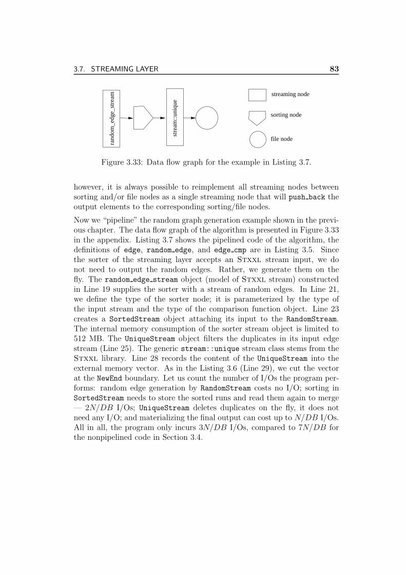
3.7. STREAMING LAYER 83
rand
om_e
dge_
stre
am
stre
am::u
niqu
e streaming node
sorting node
file node
Figure 3.33: Data flow graph for the example in Listing 3.7.
however, it is always possible to reimplement all streaming nodes betweensorting and/or file nodes as a single streaming node that will push back theoutput elements to the corresponding sorting/file nodes.
Now we “pipeline” the random graph generation example shown in the previ-ous chapter. The data flow graph of the algorithm is presented in Figure 3.33in the appendix. Listing 3.7 shows the pipelined code of the algorithm, thedefinitions of edge, random edge, and edge cmp are in Listing 3.5. Sincethe sorter of the streaming layer accepts an Stxxl stream input, we donot need to output the random edges. Rather, we generate them on thefly. The random edge stream object (model of Stxxl stream) constructedin Line 19 supplies the sorter with a stream of random edges. In Line 21,we define the type of the sorter node; it is parameterized by the type ofthe input stream and the type of the comparison function object. Line 23creates a SortedStream object attaching its input to the RandomStream.The internal memory consumption of the sorter stream object is limited to512 MB. The UniqueStream object filters the duplicates in its input edgestream (Line 25). The generic stream::unique stream class stems from theStxxl library. Line 28 records the content of the UniqueStream into theexternal memory vector. As in the Listing 3.6 (Line 29), we cut the vectorat the NewEnd boundary. Let us count the number of I/Os the program per-forms: random edge generation by RandomStream costs no I/O; sorting inSortedStream needs to store the sorted runs and read them again to merge— 2N/DB I/Os; UniqueStream deletes duplicates on the fly, it does notneed any I/O; and materializing the final output can cost up to N/DB I/Os.All in all, the program only incurs 3N/DB I/Os, compared to 7N/DB forthe nonpipelined code in Section 3.4.
84 CHAPTER 3. THE STXXL LIBRARY
Listing 3.7: Generating a random graph using the Streaming layer.
1 us ing namespace stxxl ;2 c l a s s random_edge_stream 3 int64 counter ;4 edge current ;5 random_edge_stream ( ) ;6 pub l i c :7 typede f edge value_type ;8 random_edge_stream( int64 elements ) :9 counter ( elements ) , current ( random_edge ( ) ( ) )
10 const edge & operator ∗ ( ) const r e turn current ; 11 const edge ∗ operator −>() const r e turn ¤t ; 12 random_edge_stream & operator ++ ( ) 13 −−counter ;14 current = random_edge ( ) ( ) ;15 return ∗ t h i s ;16 17 bool empty ( ) const r e turn counter==0; 18 ;19 random_edge_stream RandomStream(10000000000ULL ) ;20 typede f stream : : sort<random_edge_stream , edge_cmp>21 sorted_stream ;22 sorted_stream SortedStream( RandomStream , edge_cmp ( ) ,23 512∗1024∗1024) ;24 typede f stream : : unique<sorted_stream> unique_stream_type ;25 unique_stream_type UniqueStream( SortedStream ) ;26 stxxl : : vector<edge> ExtEdgeVec(10000000000ULL ) ;27 stxxl : : vector<edge> : : iterator NewEnd =28 stream : : materialize( UniqueStream , ExtEdgeVec . begin ( ) ) ;29 ExtEdgeVec . resize ( NewEnd − ExtEdgeVec . begin ( ) ) ;
Chapter 4
Engineering Algorithms forLarge Graphs
This chapter is devoted to engineering practical algorithms for large graphsnot fitting into the main memory. We implement the algorithms using Stxxl
and show how its features, like pipelining, help to improve the performance ofthe implementations. The performance characteristics of the implementationare tested on several architectures and on various random and real-world datasets.
4.1 Overview
We start from the simple introductory example in Section 4.2 that computesa maximal independent set of a graph. We also implement the algorithmusing the LEDA-SM library to make some conclusions about the perfor-mance. In this example the usefulness of pipelining is shown. Section 4.3engineers a practical I/O-efficient algorithm for computing minimum span-ning forests (MSF). Its performance is excellent: It is only 2–5 times slowerthan the best internal memory algorithms. The algorithm is modified in Sec-tion 4.4 to compute spanning forests (SF) and connected components (CC).The SF/CC implementation turns out to be 1.4–7.1 times faster than theMSF implementation. In Section 4.5 we compare Stxxl-implementationsof two I/O-efficient breadth first search algorithms. A simpler algorithmof Munagala and Ranade [MR99] produced bad results on difficult graphswith a large diameter. An implementation of a more involved algorithm ofMehlhorn and Meyer [MM02] has provided a better running time and I/Oguarantees for these inputs. In Section 4.6 we implement an I/O-efficient
85
86 CHAPTER 4. ENGINEERING ALGORITHMS FOR LARGE GRAPHS
algorithm for finding, counting and listing all triangles in a graph. We showthe practicality of the implementation running it on a real huge web graph.I/O-efficient algorithms for coloring graphs are studied in Section 4.7. We in-vestigate existing heuristics and develop a new fast heuristic that can 7-colorplanar graphs in O(sort(n)) I/Os.
4.2. MAXIMAL INDEPENDENT SET 87
4.2 Maximal Independent Set
We demonstrate some performance characteristics of Stxxl using the exter-nal memory maximal independent set (MIS) 1 algorithm from [Zeh02] as anexample. The MIS problem is used, for example, for scheduling dependentparallel jobs. The algorithm [Zeh02] is based on the time-forward processingtechnique. As input for the MIS algorithm we use the random graph com-puted by the examples in the previous Sections (Listings 3.6 and 3.7). Ourbenchmark also includes the running time of the input generation.
Now we describe the MIS algorithm implementation in Listing 4.1 which isonly nine lines long not including typedef declarations. The algorithm visitsthe graph nodes scanning lexicographically sorted input edges. When a nodeis visited, we add it to the maximal independent set if none of its visitedneighbors is already in the MIS. The neighbor nodes of the MIS nodes arestored as events in a priority queue. In Lines 7-9, the template metaprogram[CE00] PRIORITY QUEUE GENERATOR computes the type of priority queue thatwill store events. The metaprogram finds the optimal values for numeroustuning parameters (the number and the maximum arity of external/internalmergers, the size of merge buffers, the external memory block size, etc.) underthe constraint that the total size of the priority queue internal buffers mustbe limited by PQ MEM bytes. The node greater comparison functor definesthe order of nodes of the type node type and the minimum value that anode object can have, such that the top() method will return the smallestcontained element. The last template parameter assures that the priorityqueue cannot contain more than the INPUT SIZE elements (in 1024 units).Line 11 creates the priority queue depend having a prefetch buffer pool of sizePQ PPOOL MEM bytes and a buffered write memory pool of size PQ WPOOL MEM
bytes. The external vector MIS stores the nodes belonging to the maximalindependent set. Ordered input edges come in the form of an Stxxl streamcalled edges. If the current node edges->src is not a neighbor of a MISnode (the comparison with the current event depend.top(), Line 16), thenit is included in MIS (if it was not there before, Line 18). All neighbornodes edges->dst of a node in MIS edges->src are inserted in the eventpriority queue depend (Line 19). Lines 14-15 remove the events alreadypassed through from the priority queue.
To make a comparison with other external memory libraries, we have im-
1 An independent set I is a set of nodes on a (multi)graph G such that no edge inG joins two nodes in I, i.e. the nodes in I are not neighbors. A maximal independentset is an independent set such that adding any other node would cause the set not to beindependent anymore.
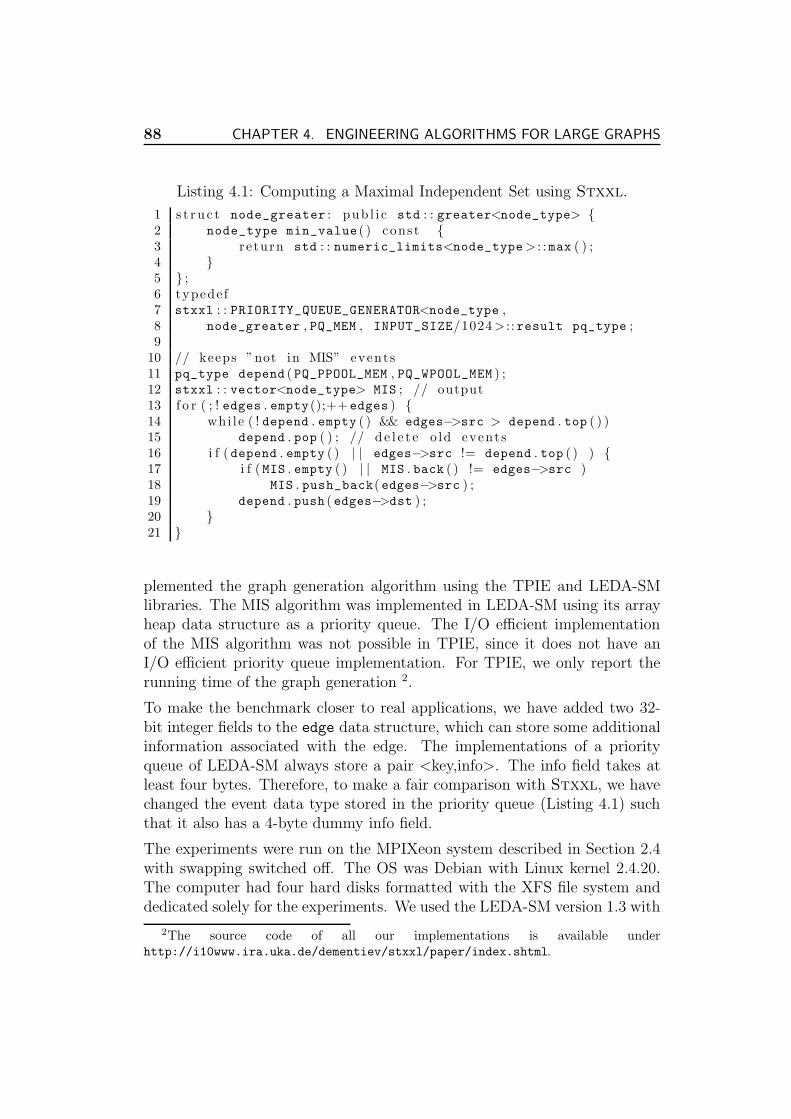
88 CHAPTER 4. ENGINEERING ALGORITHMS FOR LARGE GRAPHS
Listing 4.1: Computing a Maximal Independent Set using Stxxl.
1 s t r u c t node_greater : pub l i c std : : greater<node_type> 2 node_type min_value ( ) const 3 return std : : numeric_limits<node_type> : : max ( ) ;4 5 ;6 typede f7 stxxl : : PRIORITY_QUEUE_GENERATOR<node_type ,8 node_greater , PQ_MEM , INPUT_SIZE/1024 > : :result pq_type ;9
10 // keeps ”not in MIS” events11 pq_type depend ( PQ_PPOOL_MEM , PQ_WPOOL_MEM ) ;12 stxxl : : vector<node_type> MIS ; // output13 f o r ( ; ! edges . empty();++edges ) 14 whi le ( ! depend . empty ( ) && edges−>src > depend . top ( ) )15 depend . pop ( ) ; // d e l e t e o ld events16 i f ( depend . empty ( ) | | edges−>src != depend . top ( ) ) 17 i f ( MIS . empty ( ) | | MIS . back ( ) != edges−>src )18 MIS . push_back( edges−>src ) ;19 depend . push ( edges−>dst ) ;20 21
plemented the graph generation algorithm using the TPIE and LEDA-SMlibraries. The MIS algorithm was implemented in LEDA-SM using its arrayheap data structure as a priority queue. The I/O efficient implementationof the MIS algorithm was not possible in TPIE, since it does not have anI/O efficient priority queue implementation. For TPIE, we only report therunning time of the graph generation 2.
To make the benchmark closer to real applications, we have added two 32-bit integer fields to the edge data structure, which can store some additionalinformation associated with the edge. The implementations of a priorityqueue of LEDA-SM always store a pair <key,info>. The info field takes atleast four bytes. Therefore, to make a fair comparison with Stxxl, we havechanged the event data type stored in the priority queue (Listing 4.1) suchthat it also has a 4-byte dummy info field.
The experiments were run on the MPIXeon system described in Section 2.4with swapping switched off. The OS was Debian with Linux kernel 2.4.20.The computer had four hard disks formatted with the XFS file system anddedicated solely for the experiments. We used the LEDA-SM version 1.3 with
2The source code of all our implementations is available underhttp://i10www.ira.uka.de/dementiev/stxxl/paper/index.shtml.
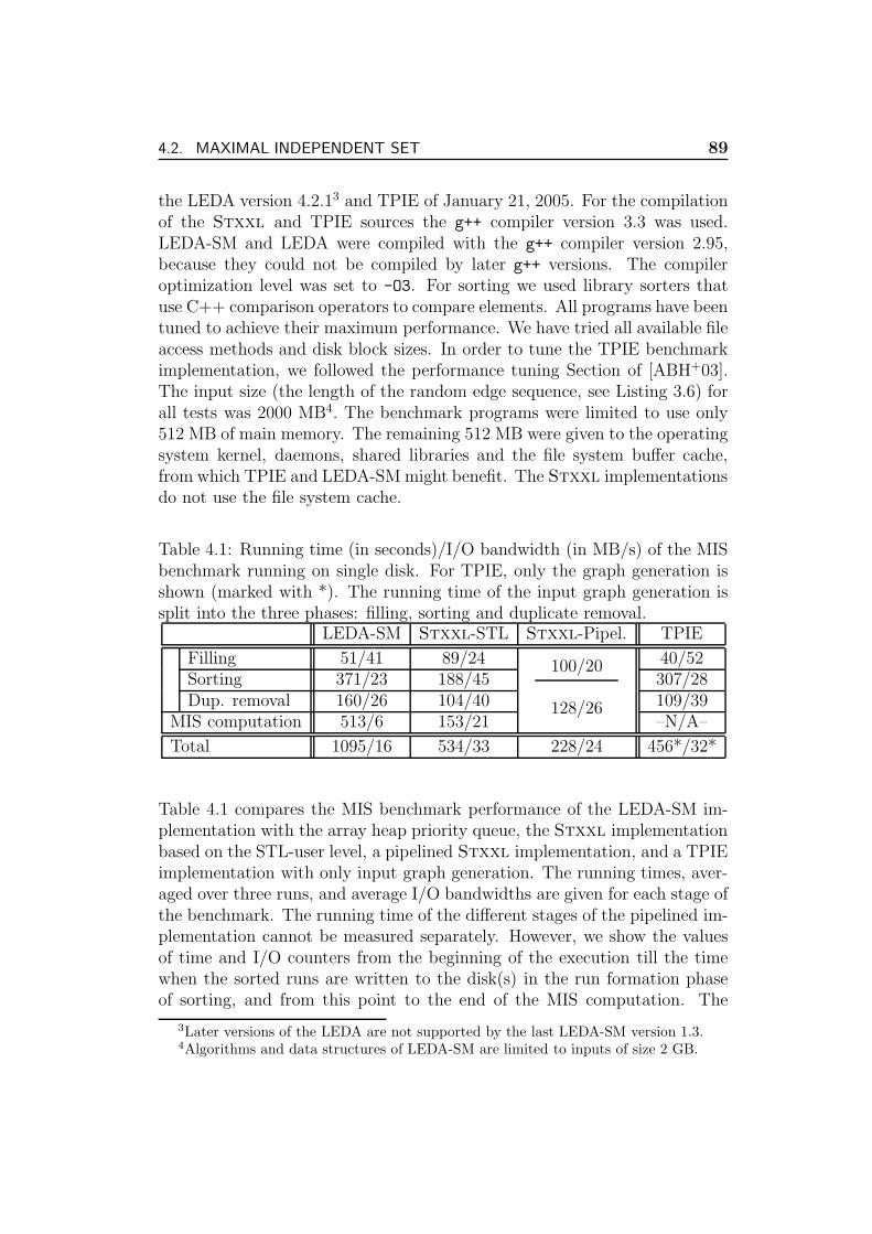
4.2. MAXIMAL INDEPENDENT SET 89
the LEDA version 4.2.13 and TPIE of January 21, 2005. For the compilationof the Stxxl and TPIE sources the g++ compiler version 3.3 was used.LEDA-SM and LEDA were compiled with the g++ compiler version 2.95,because they could not be compiled by later g++ versions. The compileroptimization level was set to -O3. For sorting we used library sorters thatuse C++ comparison operators to compare elements. All programs have beentuned to achieve their maximum performance. We have tried all available fileaccess methods and disk block sizes. In order to tune the TPIE benchmarkimplementation, we followed the performance tuning Section of [ABH+03].The input size (the length of the random edge sequence, see Listing 3.6) forall tests was 2000 MB4. The benchmark programs were limited to use only512 MB of main memory. The remaining 512 MB were given to the operatingsystem kernel, daemons, shared libraries and the file system buffer cache,from which TPIE and LEDA-SM might benefit. The Stxxl implementationsdo not use the file system cache.
Table 4.1: Running time (in seconds)/I/O bandwidth (in MB/s) of the MISbenchmark running on single disk. For TPIE, only the graph generation isshown (marked with *). The running time of the input graph generation issplit into the three phases: filling, sorting and duplicate removal.
LEDA-SM Stxxl-STL Stxxl-Pipel. TPIE
Filling 51/41 89/24 40/52Sorting 371/23 188/45
100/20307/28
Dup. removal 160/26 104/40 109/39MIS computation 513/6 153/21
128/26–N/A–
Total 1095/16 534/33 228/24 456*/32*
Table 4.1 compares the MIS benchmark performance of the LEDA-SM im-plementation with the array heap priority queue, the Stxxl implementationbased on the STL-user level, a pipelined Stxxl implementation, and a TPIEimplementation with only input graph generation. The running times, aver-aged over three runs, and average I/O bandwidths are given for each stage ofthe benchmark. The running time of the different stages of the pipelined im-plementation cannot be measured separately. However, we show the valuesof time and I/O counters from the beginning of the execution till the timewhen the sorted runs are written to the disk(s) in the run formation phaseof sorting, and from this point to the end of the MIS computation. The
3Later versions of the LEDA are not supported by the last LEDA-SM version 1.3.4Algorithms and data structures of LEDA-SM are limited to inputs of size 2 GB.
90 CHAPTER 4. ENGINEERING ALGORITHMS FOR LARGE GRAPHS
total running time numbers show that the pipelined Stxxl implementationis significantly faster than the other implementations. It is 2.4 times fasterthan the second leading implementation (Stxxl-STL). The win is due tothe reduced I/O volume: the Stxxl-STL implementation transfers 17 GB,the pipelined implementation only needs 5.2 GB. However, the 3.25 fold I/Ovolume reduction does not imply equal reduction of the running time becausethe run formation fused with the filling/generating phase becomes compute-bound. This is indicated by the almost zero value of the Stxxl I/O waitcounter, which measures the time the processing thread waited for the com-pletion of an I/O. The second reason is that the fusion of merging, duplicateremoval and CPU intensive priority queue operations in the MIS computa-tion is almost compute-bound. Comparing the running times of the totalinput graph generation, we conclude that the Stxxl-STL implementation isabout 20 % faster than TPIE and 53 % faster than LEDA-SM. This could bedue to better (explicit) overlapping between I/O and computation. Anotherpossible reason could be that TPIE uses a more expensive way of reportingrun-time errors, such as I/O errors5. The running time of the the filling stageof the Stxxl-STL implementation is much higher than that of TPIE andLEDA-SM. This is due to the fact that those libraries rely on the operatingsystem cache. The filled blocks do not go to the disk(s) immediately but re-main in the main memory until other data needs to be cached by the system.An indication for this is the very high bandwidth of 52 MB/s for the TPIEimplementation, which is even higher than the maximum physical disk band-width (48 MB/s) at its outermost zone. However, the cached blocks need tobe flushed in the sorting stage and then the TPIE implementation pays theremaining due. The unsatisfactory bandwidth of 24 MB/s of the Stxxl-STLfilling phase could be improved by replacing the call std::generate by thenative stxxl::generate call that efficiently overlaps I/O and computation.With a single disk it fills the vector in 60 seconds with a bandwidth of 33MB/s. The Stxxl STL-user sorter sustains an I/O bandwidth of about 45MB/s which is 95 % of the disk’s peak bandwidth. The high CPU load inthe priority queue and the less then perfect overlapping between I/O andcomputation explain the low bandwidth of the MIS computation stage in allthree implementations. We also run the graph generation test on 16 GByteinputs. All implementations scale with the input size almost linearly: the
5TPIE uses function return types for error codes and diagnostics, which can becomequite expensive at the level of single-item interfaces (e.g. read item and write item) thatare predominantly used in TPIEs algorithms. Instead, Stxxl checks (I/O) errors on aper-block basis. We will use C++ exceptions to propagate errors to the user layer withoutany disadvantage for the library users. First experiments indicate that this will have annegligible impact on runtime.
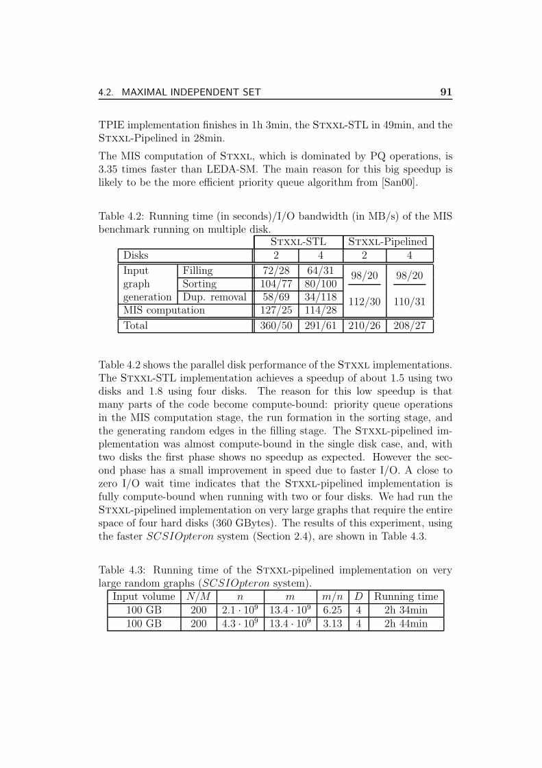
4.2. MAXIMAL INDEPENDENT SET 91
TPIE implementation finishes in 1h 3min, the Stxxl-STL in 49min, and theStxxl-Pipelined in 28min.
The MIS computation of Stxxl, which is dominated by PQ operations, is3.35 times faster than LEDA-SM. The main reason for this big speedup islikely to be the more efficient priority queue algorithm from [San00].
Table 4.2: Running time (in seconds)/I/O bandwidth (in MB/s) of the MISbenchmark running on multiple disk.
Stxxl-STL Stxxl-PipelinedDisks 2 4 2 4
Input Filling 72/28 64/31graph Sorting 104/77 80/100
98/20 98/20
generation Dup. removal 58/69 34/118MIS computation 127/25 114/28
112/30 110/31
Total 360/50 291/61 210/26 208/27
Table 4.2 shows the parallel disk performance of the Stxxl implementations.The Stxxl-STL implementation achieves a speedup of about 1.5 using twodisks and 1.8 using four disks. The reason for this low speedup is thatmany parts of the code become compute-bound: priority queue operationsin the MIS computation stage, the run formation in the sorting stage, andthe generating random edges in the filling stage. The Stxxl-pipelined im-plementation was almost compute-bound in the single disk case, and, withtwo disks the first phase shows no speedup as expected. However the sec-ond phase has a small improvement in speed due to faster I/O. A close tozero I/O wait time indicates that the Stxxl-pipelined implementation isfully compute-bound when running with two or four disks. We had run theStxxl-pipelined implementation on very large graphs that require the entirespace of four hard disks (360 GBytes). The results of this experiment, usingthe faster SCSIOpteron system (Section 2.4), are shown in Table 4.3.
Table 4.3: Running time of the Stxxl-pipelined implementation on verylarge random graphs (SCSIOpteron system).
Input volume N/M n m m/n D Running time100 GB 200 2.1 · 109 13.4 · 109 6.25 4 2h 34min100 GB 200 4.3 · 109 13.4 · 109 3.13 4 2h 44min
92 CHAPTER 4. ENGINEERING ALGORITHMS FOR LARGE GRAPHS
4.3 Minimum Spanning Trees
The results presented in this section were partially published in [DSSS04]and in the bachelor thesis [Sch03a].
4.3.1 Definitions
A spanning tree of a connected undirected graph G = (V, E) is a connectedacyclic subgraph T = (V, E ′), E ′ ⊆ E that contains all nodes of G. Given aweight function w : E → N0, the weight of a spanning tree is the sum of theweights of all edges belonging to it: w(T ) =
∑
e∈E′ w(e). A minimum span-ning tree (MST) is a spanning tree with the smallest weight over all possiblespanning trees. Graphs having several connected components cannot have asingle spanning tree, but a spanning forest, which consists of trees spanningthe connected components. Analogously, a minimum spanning forest (MSF)has the smallest weight over all spanning forests.
4.3.2 Related Work and Motivation
The problem of finding an MST (or MSF) has already been mentioned in1926 by Boruvka [Bor26]. His goal was to find an efficient electrical coverageof Bohemia. MST can be used to model many other kinds of minimum costnetwork coverage problems. Many graph algorithms need an MST computa-tion as a subroutine.
The MST problem can be solved in internal memory very efficiently. Re-cently, Pettie and Ramachandran [PR00] have found a provably optimal de-terministic MST algorithm. However, the running time complexity of thisalgorithm is unknown, it is a long standing open problem. Like the algo-rithm of Chazelle [Cha00], the algorithm of Pettie and Ramachandran hascomplexity O(mα(m, n)), where α is the inverse Ackermann function. Thefunction α grows extremely slowly, so that for all practical purposes it maybe considered a constant no greater than 4. Thus these algorithms can beconsidered to run in time very close to linear. Randomized MST algorithmsare known that run in linear expected time.
MST is one of the rare graph problems that can be solved I/O-efficiently.Using a randomized algorithm a MST can be found in O(sort(m)) expectedI/Os [ABW02]. The best known deterministic algorithm finds a MST usingO(sort(m) · max1, log log(nBD/m)) I/Os [MR99]. The deterministic lowerbound for the number of I/Os is unknown, too.
4.3. MINIMUM SPANNING TREES 93
Despite the fact that a number of I/O-efficient MST algorithms exist, noneof them has ever been implemented. A reason for that may be that even thesimplest algorithms turned out to be difficult to implement. The authors of[DSSS04] developed a simple I/O-efficient algorithm for computing MSTs ofvery large graphs. In the following we describe this algorithm as well as itstwo Stxxl implementations.
The algorithm consists of two phases. The first phase (Section 4.3.4) re-duces the node set of the input graphs until the number of nodes reachesn′ = O(M), simultaneously outputting some MST edges. For this phaseone has two implementations: an implementation for graphs with arbitrarynode degrees, based on stxxl::priority queue, and a faster bucket imple-mentation that works if the node degree is limited by O(M). In the secondphase (Section 4.3.3) the main memory can hold a constant size per-nodeinformation, thus the algorithm can operate in semi-external mode 6. Therest of the MST edges is then output. Section 4.3.5 presents the performancecharacteristics of the algorithm implementation on various families of sparserandom graphs.
4.3.3 Semi-External Algorithm
This algorithm is a variant of Kruskal’s algorithm [Kru56]. It processesthe edges in order of increasing weight. To sort the edges by weight,stxxl::ksort is used (Section 3.5). This sorter version is faster thanstxxl::sort because it can take advantage of the integer weights with re-spect to the internal work. During processing, the algorithm maintains aminimum spanning forest F of the edges seen so far. If an edge (u, v) joinstwo spanning trees in F then it is output as MST edge, otherwise it is dis-carded. The necessary operations can be implemented very efficiently usinga union-find data structure [Tar75] if nodes are numbered 0..n−1. This datastructure has been implemented using an array of integer tree links and anarray of merging ranks, both having n entries. The paper [DSSS04] showshow to dispense with the merging rank array.
4.3.4 Node Reduction
The node reduction algorithm is based on edge contraction. In each stepa random node v is chosen from the graph, and the lightest edge (v, w)
6Semi-external graph algorithms are the algorithms which operate I/O-efficiently forgraphs with n = O(M).
94 CHAPTER 4. ENGINEERING ALGORITHMS FOR LARGE GRAPHS
incident to v is found. Edge (v, w) is output as an MST edge. Node v isremoved from the graph and all its incident edges (v, u) are replaced withedges (w, u) (relinking), i.e. nodes v and w are contracted. Since the nodesare renamed during the processing, one keeps the original edge id in the edgedata structure to obtain the original ids in the MST output.
The expected number of edges inspected till the number of nodes is reduced ton′ by this abstract algorithm is bounded by 2m ln n
n′(see [DSSS04] for details
of the proof). Instead of choosing the node to delete at random the I/O-efficient implementation fixes the order of nodes in advance. If the nodes arenumbered 0..n−1 one renames the node ids using a random permutation π :0..n−1 → 0..n−1. Then the nodes are removed in the order n−1, n−2, . . . , n′.One can prove that this approach is equivalent to random sampling [DSSS04].
Priority Queue Implementation
The above mentioned algorithm easily can be implemented using an I/O-efficient priority queue. Our implementation uses stxxl::priority queue
from Section 3.4.5. Edges are stored in the form ((u, v), c, eold), where (u, v)is the edge in the current graph, c is the weight of the edge and eold isthe original id of the edge. The queue stores edges (u, v) with u > v withthe order defined as ((u, v), c, eold) < ((u′, v′), c′, e′old) iff u > u′ or u = u′ andc < c′. Using these conventions the algorithm shown in Figure 4.1 reduces thenode set to n′ nodes and outputs the MST edges performing O
(
sort(m) ln nn′
)
I/Os [DSSS04]. The real code [Sch03a] that implements the pseudocode usingStxxl is very short and simple: the reduction is programmed using only12 lines of C++ code (see Listing 4.2).
Bucket Implementation
The priority queue implementation has a substantional internal CPU workoverhead since it unnecessarily sorts the edges within the adjacency list ofa node. However, one should assure that the lightest edge comes first. Theauthors of the paper [DSSS04] propose an implementation of the reductionphase that has linear work in the total I/O volume.
As in the PQ implementation, in iteration i node i is removed by outputtingthe lightest edge incident to it and relinking all the other edges. The edges(u, v), v < u ∧ n′ < u ≤ n − 1 are stored in k equal sized external memorybuckets, where k = O(M/B). The remaining edges (u, v), v < u, u ∈ [0, n′)are stored in a special external memory bucket. This bucket is implemented
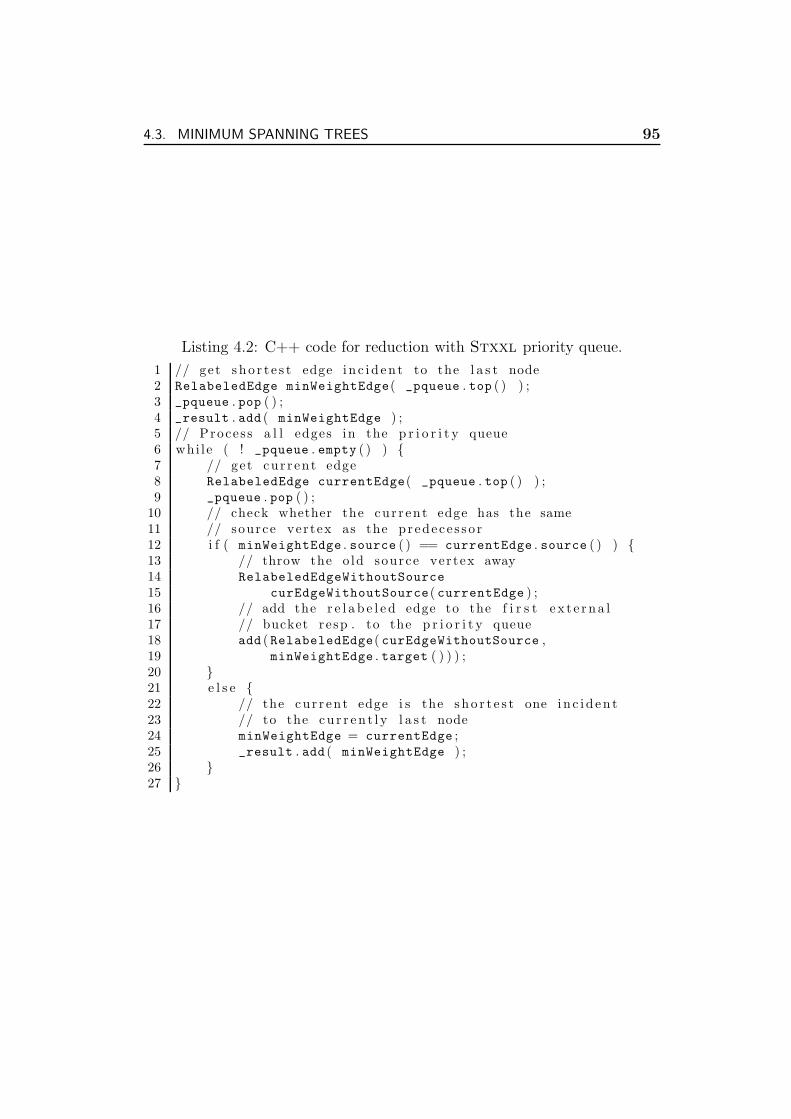
4.3. MINIMUM SPANNING TREES 95
Listing 4.2: C++ code for reduction with Stxxl priority queue.
1 // get s ho r t e s t edge i n c i d en t to the l a s t node2 RelabeledEdge minWeightEdge( _pqueue . top ( ) ) ;3 _pqueue . pop ( ) ;4 _result . add ( minWeightEdge ) ;5 // Proces s a l l edges in the p r i o r i t y queue6 whi le ( ! _pqueue . empty ( ) ) 7 // get cur r ent edge8 RelabeledEdge currentEdge( _pqueue . top ( ) ) ;9 _pqueue . pop ( ) ;
10 // check whether the cur r ent edge has the same11 // source ver tex as the pr edece s so r12 i f ( minWeightEdge . source ( ) == currentEdge . source ( ) ) 13 // throw the o ld source ver tex away14 RelabeledEdgeWithoutSource
15 curEdgeWithoutSource( currentEdge ) ;16 // add the r e l a b e l e d edge to the f i r s t e x t e r na l17 // bucket resp . to the p r i o r i t y queue18 add ( RelabeledEdge( curEdgeWithoutSource ,19 minWeightEdge . target ( ) ) ) ;20 21 e l s e 22 // the cur r ent edge i s the s ho r t e s t one i n c i d en t23 // to the cu r r en t l y l a s t node24 minWeightEdge = currentEdge ;25 _result . add ( minWeightEdge ) ;26 27
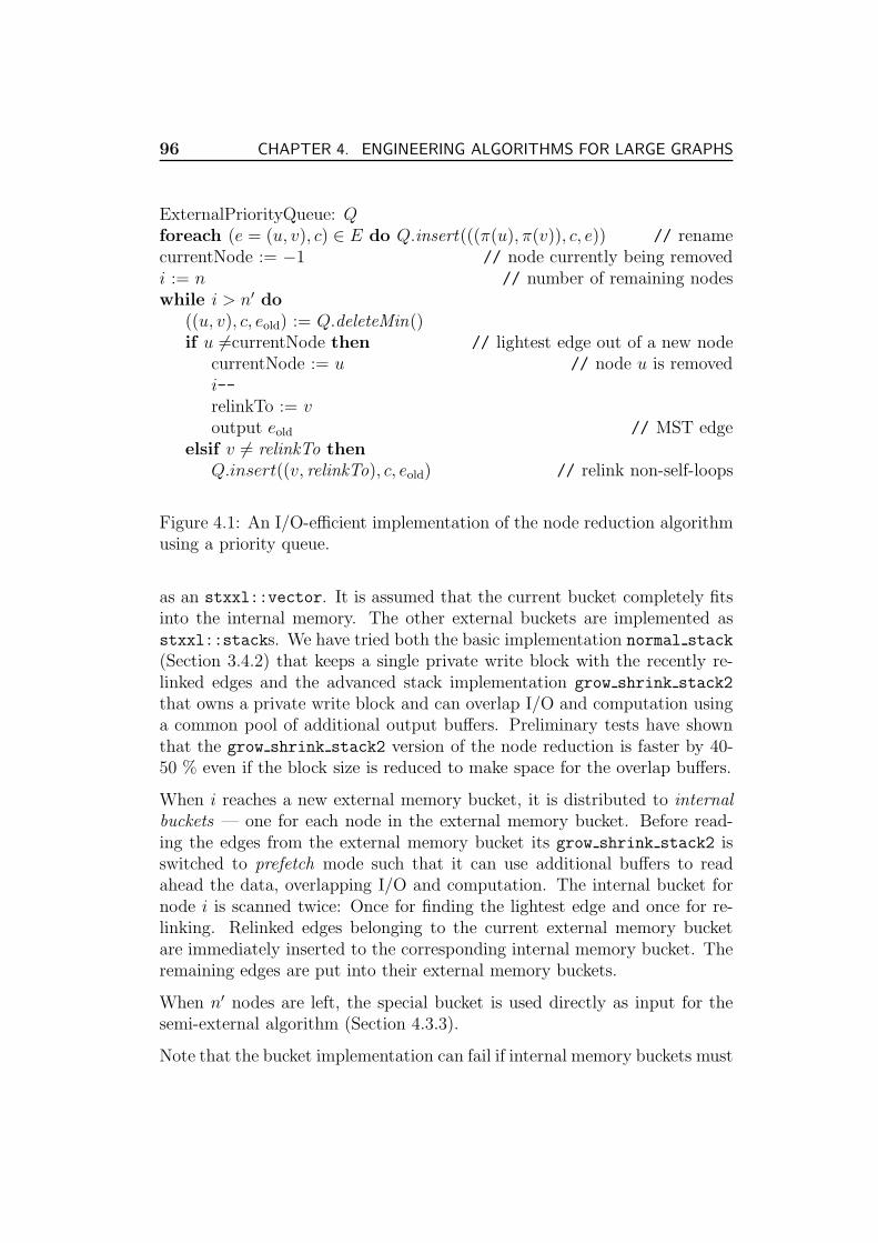
96 CHAPTER 4. ENGINEERING ALGORITHMS FOR LARGE GRAPHS
ExternalPriorityQueue: Qforeach (e = (u, v), c) ∈ E do Q.insert(((π(u), π(v)), c, e)) // renamecurrentNode := −1 // node currently being removedi := n // number of remaining nodeswhile i > n′ do
((u, v), c, eold) := Q.deleteMin()if u 6=currentNode then // lightest edge out of a new node
currentNode := u // node u is removedi--relinkTo := voutput eold // MST edge
elsif v 6= relinkTo thenQ.insert((v, relinkTo), c, eold) // relink non-self-loops
Figure 4.1: An I/O-efficient implementation of the node reduction algorithmusing a priority queue.
as an stxxl::vector. It is assumed that the current bucket completely fitsinto the internal memory. The other external buckets are implemented asstxxl::stacks. We have tried both the basic implementation normal stack
(Section 3.4.2) that keeps a single private write block with the recently re-linked edges and the advanced stack implementation grow shrink stack2
that owns a private write block and can overlap I/O and computation usinga common pool of additional output buffers. Preliminary tests have shownthat the grow shrink stack2 version of the node reduction is faster by 40-50 % even if the block size is reduced to make space for the overlap buffers.
When i reaches a new external memory bucket, it is distributed to internalbuckets — one for each node in the external memory bucket. Before read-ing the edges from the external memory bucket its grow shrink stack2 isswitched to prefetch mode such that it can use additional buffers to readahead the data, overlapping I/O and computation. The internal bucket fornode i is scanned twice: Once for finding the lightest edge and once for re-linking. Relinked edges belonging to the current external memory bucketare immediately inserted to the corresponding internal memory bucket. Theremaining edges are put into their external memory buckets.
When n′ nodes are left, the special bucket is used directly as input for thesemi-external algorithm (Section 4.3.3).
Note that the bucket implementation can fail if internal memory buckets must
4.3. MINIMUM SPANNING TREES 97
hold adjacency list of nodes with very a high degree. [DSSS04] proposessolutions for this problem, namely, it is possible to move the high-degreenodes from the internal bucket to the special bucket and even if the averagesize external bucket does not fit into the internal memory then one can applya multi-level distribution scheme. As an option for problem buckets one couldalso temporarily switch to the priority queue implementation.
Parallel Edges and Sparse Graphs
The node reduction algorithm described earlier can produce parallel edgesduring relinking. Moreover, these edges also remain in the graph after subse-quent relinking operations. However, they can be removed relatively easily.While scanning the internal buckets the edges (u, v) are put into an interme-diate hash table before before moving them to the appropriate buckets. Notethat this hash table only keeps the lightest edge between the nodes u and vseen so far. When the capacity of the hash table is reached or all nodes inthe current external bucket are scanned, the edges accumulated in the hashtable are flushed to the buckets.
[DSSS04] proves that this simple treatment reduces the I/O complexity of thealgorithm to O(sort(n)) I/Os for planar graphs, graphs with a bounded tree-width and other families of graphs that remain sparse under edge contraction.
Implementation Details
The implementation of the internal buckets is very efficient both in runningtime and space consumption. They are represented as linked lists of smallblocks that can hold several edges each. An edge structure stored in aninternal bucket does not keep the source node id because this information isredundant. In the external memory part, the edge data structure is stored asa 5-tuple of 32-bit integers and stores the original edge id directly as two endpoints. This saves the additional sort/scan phase at the end for the restoringof the original ids of MST edges. Another advantage is that it allows togive ids to more than 232 edges in a straightforward way without needingany special coding scheme for ids greater than 232. More details about theimplementation can be found in [Sch03a].
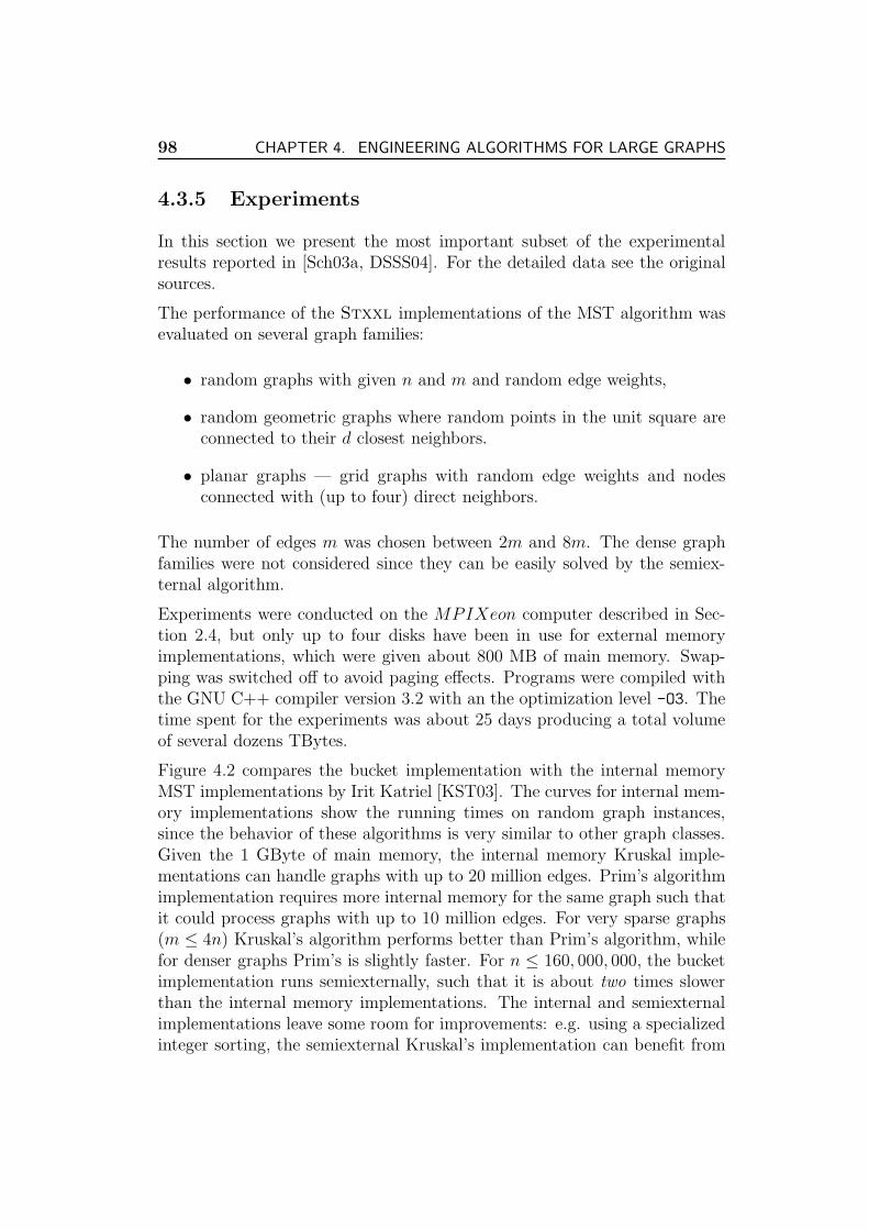
98 CHAPTER 4. ENGINEERING ALGORITHMS FOR LARGE GRAPHS
4.3.5 Experiments
In this section we present the most important subset of the experimentalresults reported in [Sch03a, DSSS04]. For the detailed data see the originalsources.
The performance of the Stxxl implementations of the MST algorithm wasevaluated on several graph families:
• random graphs with given n and m and random edge weights,
• random geometric graphs where random points in the unit square areconnected to their d closest neighbors.
• planar graphs — grid graphs with random edge weights and nodesconnected with (up to four) direct neighbors.
The number of edges m was chosen between 2m and 8m. The dense graphfamilies were not considered since they can be easily solved by the semiex-ternal algorithm.
Experiments were conducted on the MPIXeon computer described in Sec-tion 2.4, but only up to four disks have been in use for external memoryimplementations, which were given about 800 MB of main memory. Swap-ping was switched off to avoid paging effects. Programs were compiled withthe GNU C++ compiler version 3.2 with an the optimization level -O3. Thetime spent for the experiments was about 25 days producing a total volumeof several dozens TBytes.
Figure 4.2 compares the bucket implementation with the internal memoryMST implementations by Irit Katriel [KST03]. The curves for internal mem-ory implementations show the running times on random graph instances,since the behavior of these algorithms is very similar to other graph classes.Given the 1 GByte of main memory, the internal memory Kruskal imple-mentations can handle graphs with up to 20 million edges. Prim’s algorithmimplementation requires more internal memory for the same graph such thatit could process graphs with up to 10 million edges. For very sparse graphs(m ≤ 4n) Kruskal’s algorithm performs better than Prim’s algorithm, whilefor denser graphs Prim’s is slightly faster. For n ≤ 160, 000, 000, the bucketimplementation runs semiexternally, such that it is about two times slowerthan the internal memory implementations. The internal and semiexternalimplementations leave some room for improvements: e.g. using a specializedinteger sorting, the semiexternal Kruskal’s implementation can benefit from
4.3. MINIMUM SPANNING TREES 99
1
2
3
4
5
6
5 10 20 40 80 160 320 640 1280 2560
t / m
[µs]
m / 1 000 000
KruskalPrim
randomgeometric
grid
1
2
3
4
5
6
5 10 20 40 80 160 320 640 1280 2560
t / m
[µs]
m / 1 000 000
KruskalPrim
randomgeometric
1
2
3
4
5
6
5 10 20 40 80 160 320 640 1280 2560
t / m
[µs]
m / 1 000 000
KruskalPrim
randomgeometric
Figure 4.2: Execution time per edge of the bucket implementation for m ≈2 · n (top), m ≈ 4 · n (center), m ≈ 8 · n (bottom).
100 CHAPTER 4. ENGINEERING ALGORITHMS FOR LARGE GRAPHS
merging the sort and the scan part in a pipeline saving I/Os (Section 3.7).Beyond 160, 000, 000 nodes the full bucket implementation is needed. Therunning time almost doubles because of the additional costs of the node re-naming, node reduction, and a blowup of the size of the edge data structurefrom 12 to 20 bytes. As the complexity of the reduction is superlinear (Sec-tion 4.3.4), the running time keeps growing with n/M for random graphs.
The running time on grid graphs and geometric graphs is much better thanone could expect. The time per edge even decreases with m. An explanationfor this is that for these types of graphs, many parallel edges are producedand eliminated during relinking. For denser graphs less edges survive duringthe node reduction, such that the semiexternal Kruskal’s implementationprocesses unproportionally small number of edges.
The largest graph that has been tried out was a grid graph with about 232
nodes taking 96 GBytes just to represent the input (12 bytes per edge). Thisgraph was processed in a record time of about 8h 40min transferring 830GBytes of data.
The bucket implementation has been compared with the implementationbased on the stxxl::priority queue. The following small table shows therunning time in µs per edge for random graphs with n = 320 · 106 andm = 640 · 106, where we varied the number of disks:
1 disk 4 disksbucket implementation 6.7 4.3priority queue implementation 11.0 8.9
Since the speedup for the bucket algorithm after quadrupling the number ofdisks is only 1.56, one can conclude that even with a single disk and the inter-nally efficient bucket algorithm, the computation is rather CPU-bound. Sincethe bucket implementation requires less CPU work, it performs considerablybetter than the the PQ implementation. However, the PQ implementation isstill interesting because it is simple, can process graphs on which the bucketimplementation might fail, and also achieves a reasonable performance for asingle disk.
4.3.6 Conclusions
It has been demonstrated that massive minimum spanning trees filling severaldisks can be solved “overnight” on a cheap hardware. In particular, thisbecame possible due to the simple and efficient implementations that profitfrom the Stxxl library.
4.4. CONNECTED COMPONENTS AND SPANNING TREES 101
4.4 Connected Components and Spanning
Trees
In this section we show how the external memory implementations of MSTalgorithms from Section 4.3 can be modified to compute spanning forests (SF)and connected components (CC). This material is based on the extension[Sch03b] of the bachelor thesis of Schultes [Sch03a].
4.4.1 Introduction
The connected component problem on an undirected graph G = (V, E) is theproblem of finding a mapping c : V → N, such that c(v) = c(u) for v, u ∈ Viff v and u belong to the same connected component.
In the internal memory the connected component problem and the spanningforest problem can be solved in linear time O(m + n) using the Breadth-or Depth-First-Search algorithms. However, in the external memory settingthese problems can be solved only within the same asymptotic bounds as theMST problem (Section 4.3.2 and [MR99, ABW02]). No better bounds areknown.
4.4.2 Spanning Forest
The node reduction algorithm (Section 4.3) coupled with the semiexternal al-gorithm already produces a spanning forest. One can speedup this algorithmby simplifying and removing some steps of the algorithm since the outputdoes not have to be a minimum forest. The I/O volume of the node reductioncan be reduced since the weight component of the edge tuples is not neededanymore. This also leads to some saving of internal memory space of theinternal buckets. Thus, the block size of the external memory buckets can beincreased, which can affect the overall performance positively. The base case(semiexternal Kruskal’s algorithm) can be simplified as the sorting step canbe skipped. In the node reduction phase, while removing node i, instead ofchoosing the lightest adjacent edge to contract, one chooses an adjacent edge(i, v) with the smallest id v. By intuition, this is a good decision, becausethe work is postponed to later iterations and the number of nodes to processin the future reduces faster (e.g. compared to the random choice) [Sib97].
The improvements concerning the node reduction phase can be applied toboth bucket and priority queue versions. In [Sch03b] only the reduction with

102 CHAPTER 4. ENGINEERING ALGORITHMS FOR LARGE GRAPHS
buckets has been implemented since the priority queue version would havehad a similar speedup.
4.4.3 Connected Components
Schultes [Sch03b] modifies and extends the bucket version of the algorithmto perform accordingly with the algorithm described in [Sib04, SM02]. As inthe spanning forest algorithm, the input is an unweighted graph representedas a list of edges. The output of the algorithm is a list of entries (v, c), v ∈ V ,where c is the connected component id of node v, at the same time c is theid of a node belonging to the connected component. This special node c issometimes called the representative node of a component. The algorithmmakes two passes over adjacency lists of nodes (left-to-right pass v = n−1..0and right-to-left v = 0..n − 1, v ∈ V ), relinking the edges such that theyconnect node v with the representative node of its connected component.
Schultes integrates the algorithm [Sib04, SM02] into the bucket implemen-tation of the spanning forests algorithm. If there are k = O(M/B) externalmemory buckets then bucket i ∈ 0..k − 1 contains the adjacent edges(u, v), u > v of nodes ui−1 < u ≤ ui, where ui is the upper (lower) bound ofnode ids in bucket i (i + 1). Additionally, there are k question buckets andk answer buckets with the same bounds. A question is a tuple (v, r(v)) thatrepresents the assignment of node v to a preliminary representative noder(v). An answer is a tuple (v, r(v)) that represents the assignment of nodev to an ultimate representative node. Function b : V → 0..k − 1 maps anode id to the coresponding bucket id according to the bucket bounds.
The bucket implementation is complemented with the following steps. Dur-ing the processing of node v, the algorithm assigns r(v) tentatively the idof its neighbor with the smallest id. If no neighbor exists then r(v) := v.After processing the bucket i we post the preliminary assignments (v, r(v)) ofnodes v, ui−1 < v ≤ ui to question bucket b(r(v)) if r(v) does not belong tobucket i. Otherwise we can update r(v) with r(r(v)). If the new r(v) belongsto bucket i than it is the ultimate representative node of v and (v, r(v)) canbe written to the answer bucket b(v), otherwise we post question (v, r(v)) tothe appropriate question bucket. Note that the first answer bucket is handleddifferently as it is implemented as the union-find data structure in the basecase. For v in the union-data structure r(v) is the id of the leader node ofthe union where v belongs to. The connected component algorithm needs anadditional right-to-left scan to determine the ultimate representatives whichhave not been determined in the previous left-to-right scan. The buckets are

4.4. CONNECTED COMPONENTS AND SPANNING TREES 103
read in the order 0..k − 1. For each (v, r(v)) in question bucket i we updater(v) with the ultimate representative r(r(v)) looking up values in answerbucket i. The final value (v, r(v)) is appended to answer bucket b(v). Afteranswering all questions in bucket i, the content of answer bucket i is addedto the output of the connected component algorithm.
If one only needs to compute the component ids and no spanning tree edgesthen the implementation does not keep the original edge id in the edge datastructure. It is sufficient to invert randomization for the node ids in theoutput, which can be done with the chosen randomization scheme [DSSS04,Sch03a] without additional I/Os. Due to this measure the total I/O volumeand the memory requirements of the internal buckets are reduced such thatthe block size of the external memory buckets can be made larger. All thisleads to an overall performance improvement.
4.4.4 Experiments
The experiment setup including the computer system and input instanceswas the same as in the MST algorithm evaluation (Section 4.3).
Since the connected component and spanning tree algorithms are modifica-tions of the MST algorithm they show a similar development of running timewith the change in problem size and in density of the graphs. Thus we onlyshow the relative speedup of the algorithms over the MST algorithm for thesemi-external and the external case in Table 4.4. For the detailed data see[Sch03b]. Computing connected components and/or spanning forests is atleast 1.4 times faster than computing MST. The most important reason forthat is that the I/O volume is decreased: the weight field in the edge tupleis not needed and the edges are not sorted like in Kruskal’s algorithm. Thecomputation of connected components takes more time than the computationof a spanning forest mainly because it needs an additional pass through thenodes. Nethertheless SF&CC is still faster than the MST implementation.
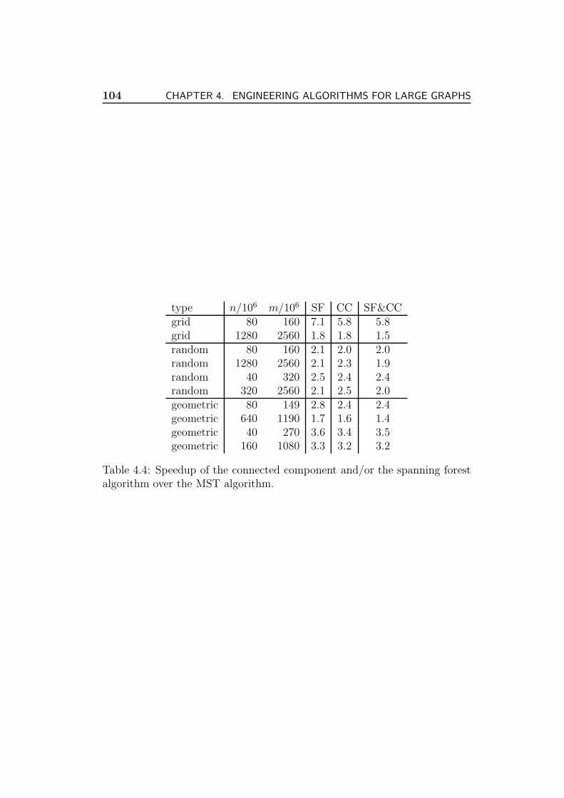
104 CHAPTER 4. ENGINEERING ALGORITHMS FOR LARGE GRAPHS
type n/106 m/106 SF CC SF&CCgrid 80 160 7.1 5.8 5.8grid 1280 2560 1.8 1.8 1.5random 80 160 2.1 2.0 2.0random 1280 2560 2.1 2.3 1.9random 40 320 2.5 2.4 2.4random 320 2560 2.1 2.5 2.0geometric 80 149 2.8 2.4 2.4geometric 640 1190 1.7 1.6 1.4geometric 40 270 3.6 3.4 3.5geometric 160 1080 3.3 3.2 3.2
Table 4.4: Speedup of the connected component and/or the spanning forestalgorithm over the MST algorithm.
4.5. BREADTH FIRST SEARCH 105
4.5 Breadth First Search
Some of the material of this section has been published in [ADM06] and inthe master’s thesis [Ajw05].
4.5.1 Introduction
Many combinatorial problems need to traverse a graph in a structured way.Breadth First Search (BFS) is one of the most useful traversal strategies. Foran undirected graph G = (V, E) and a source node s ∈ V , BFS decomposesnodes of the graph into at most n = |V | levels, where each level i containsthe nodes that can be reached from s via a path of i edges, but can not bereached using less than i edges.
In the internal memory setting, the problem of finding the BFS decomposi-tion can be solved by a simple linear time algorithm [CLR90]. In the externalmemory setting, i.e. when the input graph is too big to be processed in themain memory, this algorithm incurs Θ(n+m) I/Os. Until recently it was notclear if the exact BFS computation for such large graphs is feasible at all.Therefore heuristics (exploiting some graph properties), and special precom-putations producing approximate solutions have been developed. However,two promising I/O-efficient BFS algorithms with small constant factors bothin I/O volume and CPU-time complexity exist: the MR-BFS [MR99] andMM-BFS [MM02] algorithms.
In the remaining part of this section we show that MR-BFS and MM-BFSalgorithms implemented with Stxxl are able to compute the exact BFS-leveldecomposition for huge synthetic and real graphs in a few hours. Thanks tothe Stxxl pipelining the implementations save at least a factor two in I/O-volume.
4.5.2 Internal Memory BFS
The internal memory BFS (IM-BFS) algorithm [CLR90] visits the nodes ofthe graph sequentially, starting from the source node s. The algorithm keepsthe candidate nodes to visit in a FIFO queue Q. When a node v is extractedfrom Q, the adjacency list of v is examined and unvisited neighbors areadded to Q. This simple algorithm is not I/O-efficient due to two reasons:(1) remembering the visited nodes costs Θ(m) I/Os in the worst case; (2)unstructured accesses to the adjacency lists need up to Θ(n) I/Os.
106 CHAPTER 4. ENGINEERING ALGORITHMS FOR LARGE GRAPHS
4.5.3 MR-BFS
The MR-BFS algorithm [MR99] addresses the first problem reducing theworst case I/O-complexity to O(n + sort(n + m)). The algorithm computesthe BFS levels incrementally. Let L(t) be the set of the nodes in levelt, N(S) be the multi-set of the neighbors of the nodes in set S and letA(t) := N(L(t − 1)). The current level L(t) is constructed as follows:A(t) is created by |L(t − 1)| accesses to the adjacency lists. This incursO(|L(t − 1)| + scan(|A(t)|)) I/Os. Then the duplicate nodes are removedfrom the multi-set A(t) obtaining set A′(t) using a sorting and a scan-ning step. This needs O(sort(|A(t)|)) I/Os. L(t) can be computed nowas A′(t) − L(t − 1) ∪ L(t − 2). Filtering out the nodes contained inthe sorted sets L(t − 1) and L(t − 2) is possible by parallel scanning inO(scan(|A(t)| + |L(t − 1)| + |L(t − 2)|)) I/Os. Since
∑
t |A(t)| = 2m 7 and∑
t |L(t)| = n, the algorithm requires the O(n + sort(n + m)) I/Os. Theunstructured access to the adjacency lists of L(t − 1) is responsible for theO(n) term.
Figure 4.3 shows the scheme of the pipelined and nonpipelined implemen-tations of one MR-BFS iteration. In the pipelined version the whole algo-rithm complexity can be implemented in one scanner that reads the nodes inL(t− 1) and L(t− 1) and the adjacency lists E(t) of nodes in L(t) from thecorresponding stxxl::vectors and scans through the stream of A′(t) andin just one pass outputs the nodes in the current level L(t) and the multi-setA(t + 1), which is passed directly to the sorter. The output of the sorter isscanned once to delete duplicates and output as the set A′(t + 1) used in thenext iteration.
Analyzing the schemes we conclude 8 that pipelining reduces the worst casenumber of I/Os from∑
t scan(|L(t − 1)| + |L(t − 2)| + |A(t)|) +∑
t 2 scan(|L(t)|) +∑
t(|L(t)| + scan(|N(L(t))|) +∑
t 2 scan(|A(t + 1)|) +∑
t(sort(|A(t + 1)|) + 3 scan(|A(t + 1)|)) = n + scan(4n + 14m) + sort(2m)
to∑
t scan(|L(t − 1)| + |L(t − 2)|) +∑
t(|L(t)| + scan(|N(L(t))|) +
7Note that graph is undirected and each edge is stored twice.8To simplify the analysis the record size is assumed to be equal in all data streams.

4.5. BREADTH FIRST SEARCH 107
N(L(t))
N(L(t))
L(t−1)
L(t)E(t)
L(t−2) A’(t)
sort
L(t−1) L(t−2)
E(t)
sort
A’(t)
L(t)
compute A´(t)−L(t−1)−L(t−2)
find neighbors of L(t)
remove dupl.
parallel scan
Figure 4.3: Scheme of the MR-BFS algorithm: nonpipelined (left) andpipelined (right).
∑
t scan(|L(t)|) +∑
t sort(|A(t + 1)|) = n + scan(3n + 2m) + sort(2m).
Assuming that sort(x) = 2 · scan(x) with a careful choice of block size B weconclude that pipelining can save at least half of the required I/O volume(ignoring the worst case n term).
4.5.4 MM-BFS
The MM-BFS algorithm [MM02] is a refinement of the MR-BFS algorithmthat trades in the unstructured I/O for the increase of the number of itera-tions in which an edge may be involved. On sparse graphs the total amountof the unstructured I/O can be reduced by a factor of up to
√B. MM-BFS
runs in two phases: a preprocessing phase that partitions the graph into dis-joint clusters and the BFS phase itself. In [MM02], deterministic and nonde-terministic variants of preprocessing have been proposed. [ADM06, Ajw05]implements the simpler randomized version.
108 CHAPTER 4. ENGINEERING ALGORITHMS FOR LARGE GRAPHS
In order to efficiently store the graph partition the following graph repre-sentation has been designed. The adjacency array is implemented as twostxxl::vectors V and E. Vector E contains all edges of the graph twice– once in the adjacency array of each adjacent node. Vector V contains theiterators pointing to locations in E where a new adjacency array starts. Anstxxl::vector F stores the iterators to locations in V marking the firstnode of clusters, i.e. nodes pointed by F [i], F [i] + 1, . . . , F [i + 1] − 1 buildcluster Fi. Edges and nodes in V and E are kept sorted according to thecluster indices they belong to. Using this representation an arbitrary clustercan be accessed in O(1) + scan(F [i + 1] − F [i]) I/Os.
The preprocessing step partitions the graph into disjoint connected subgraphsSi, 0 ≤ i ≤ K, with a small expected diameter [MM02]. It also partitions theadjacency arrays accordingly, i.e. it constructs vector F and reorganizes Vand E accordingly, such that cluster Fi contains the adjacency arrays of allnodes in Si. We assume that S0 contains the source node s. The partition isbuilt by choosing master nodes independently and uniformly at random with
a probability µ =√
(n+m) log nnDB
and running a local BFS from all master nodes
“in parallel”: in each round, each master node si tries to capture all unvisitedneighbors of its current subgraph Si; this is done by first sorting the nodesof the active fringes of all Si, and then scanning the dynamically shrinkingadjacency-array representation of the yet unexplored graph. If several masternodes want to include a certain node, an arbitrary master nodes wins.
After choosing master nodes, the partitioning can run in pipelined modeas shown in Figure 4.3 (left). The top scanner takes the sorted sequenceof the nodes on the fringe, updates their cluster ids in the external vectorV , adding them to the corresponding cluster. In the same scanner, adja-cency lists of the fringe nodes are read and a new sequence of fringe nodesis determined. The sequence is sent then to the sorter. After partitioning,we generate the graph data structure described above. For this purpose,each edge in E is supplemented with source and destination node clusterids. Sorted with respect to cluster ids, E and V are scanned to produce theappropriate node and cluster iterator values. According to the analysis in[MM02] the diameter of any cluster (the number of iterations) is less thanlog n
µwith high probability. Thus the total number of I/Os for the partitioning
is log nµ
(scan(2m) + sort(2n)) + scan(4n + µn + 4m) + sort(4m + n).
In the BFS phase the algorithm performs similarly to the MR-BFS with onedifference: the adjacency arrays are not accessed directly, but cached in aspecial pool H (“hot” adjacency arrays). The hot pool contains parts of thecluster adjacency arrays Fi if Fi has a node in level L(t−1). Pool H initially
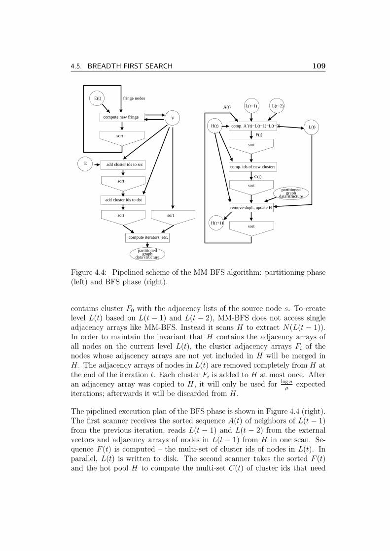
4.5. BREADTH FIRST SEARCH 109
sort
sort
sort sort
graphpartitioned
data structure
graphpartitioned
data structure
E(t)
E
fringe nodes
sort
L(t−1) L(t−2)
sort
sort
L(t)H(t)
H(t+1)
A(t)
F(t)
C(t)
compute new fringe
add cluster ids to src
add cluster ids to dst
compute iterators, etc.
comp. A´(t)−L(t−1)−L(t−2)
comp. ids of new clusters
remove dupl., update H
V
Figure 4.4: Pipelined scheme of the MM-BFS algorithm: partitioning phase(left) and BFS phase (right).
contains cluster F0 with the adjacency lists of the source node s. To createlevel L(t) based on L(t − 1) and L(t − 2), MM-BFS does not access singleadjacency arrays like MM-BFS. Instead it scans H to extract N(L(t − 1)).In order to maintain the invariant that H contains the adjacency arrays ofall nodes on the current level L(t), the cluster adjacency arrays Fi of thenodes whose adjacency arrays are not yet included in H will be merged inH . The adjacency arrays of nodes in L(t) are removed completely from H atthe end of the iteration t. Each cluster Fi is added to H at most once. Afteran adjacency array was copied to H , it will only be used for log n
µexpected
iterations; afterwards it will be discarded from H .
The pipelined execution plan of the BFS phase is shown in Figure 4.4 (right).The first scanner receives the sorted sequence A(t) of neighbors of L(t − 1)from the previous iteration, reads L(t − 1) and L(t − 2) from the externalvectors and adjacency arrays of nodes in L(t − 1) from H in one scan. Se-quence F (t) is computed – the multi-set of cluster ids of nodes in L(t). Inparallel, L(t) is written to disk. The second scanner takes the sorted F (t)and the hot pool H to compute the multi-set C(t) of cluster ids that need
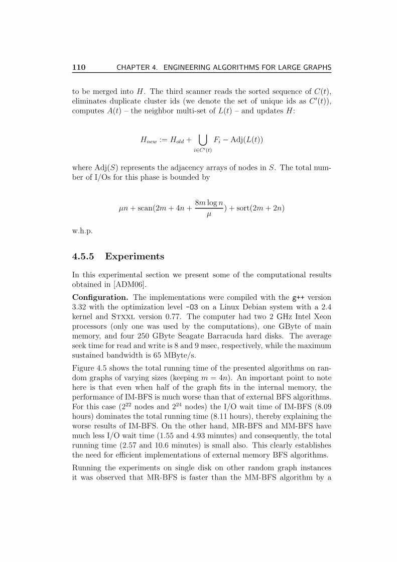
110 CHAPTER 4. ENGINEERING ALGORITHMS FOR LARGE GRAPHS
to be merged into H . The third scanner reads the sorted sequence of C(t),eliminates duplicate cluster ids (we denote the set of unique ids as C ′(t)),computes A(t) – the neighbor multi-set of L(t) – and updates H :
Hnew := Hold +⋃
i∈C′(t)
Fi − Adj(L(t))
where Adj(S) represents the adjacency arrays of nodes in S. The total num-ber of I/Os for this phase is bounded by
µn + scan(2m + 4n +8m log n
µ) + sort(2m + 2n)
w.h.p.
4.5.5 Experiments
In this experimental section we present some of the computational resultsobtained in [ADM06].
Configuration. The implementations were compiled with the g++ version3.32 with the optimization level -O3 on a Linux Debian system with a 2.4kernel and Stxxl version 0.77. The computer had two 2 GHz Intel Xeonprocessors (only one was used by the computations), one GByte of mainmemory, and four 250 GByte Seagate Barracuda hard disks. The averageseek time for read and write is 8 and 9 msec, respectively, while the maximumsustained bandwidth is 65 MByte/s.
Figure 4.5 shows the total running time of the presented algorithms on ran-dom graphs of varying sizes (keeping m = 4n). An important point to notehere is that even when half of the graph fits in the internal memory, theperformance of IM-BFS is much worse than that of external BFS algorithms.For this case (222 nodes and 224 nodes) the I/O wait time of IM-BFS (8.09hours) dominates the total running time (8.11 hours), thereby explaining theworse results of IM-BFS. On the other hand, MR-BFS and MM-BFS havemuch less I/O wait time (1.55 and 4.93 minutes) and consequently, the totalrunning time (2.57 and 10.6 minutes) is small also. This clearly establishesthe need for efficient implementations of external memory BFS algorithms.
Running the experiments on single disk on other random graph instancesit was observed that MR-BFS is faster than the MM-BFS algorithm by a
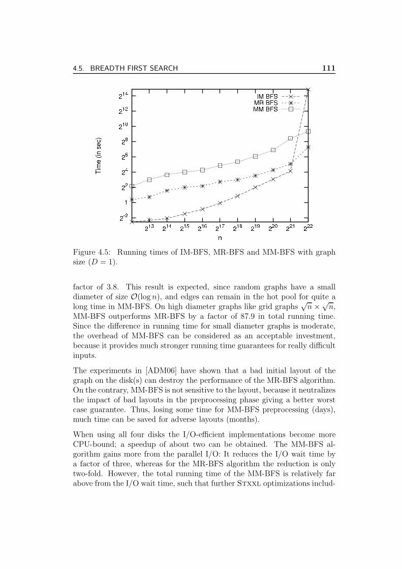
4.5. BREADTH FIRST SEARCH 111
Figure 4.5: Running times of IM-BFS, MR-BFS and MM-BFS with graphsize (D = 1).
factor of 3.8. This result is expected, since random graphs have a smalldiameter of size O(log n), and edges can remain in the hot pool for quite along time in MM-BFS. On high diameter graphs like grid graphs
√n ×√
n,MM-BFS outperforms MR-BFS by a factor of 87.9 in total running time.Since the difference in running time for small diameter graphs is moderate,the overhead of MM-BFS can be considered as an acceptable investment,because it provides much stronger running time guarantees for really difficultinputs.
The experiments in [ADM06] have shown that a bad initial layout of thegraph on the disk(s) can destroy the performance of the MR-BFS algorithm.On the contrary, MM-BFS is not sensitive to the layout, because it neutralizesthe impact of bad layouts in the preprocessing phase giving a better worstcase guarantee. Thus, losing some time for MM-BFS preprocessing (days),much time can be saved for adverse layouts (months).
When using all four disks the I/O-efficient implementations become moreCPU-bound; a speedup of about two can be obtained. The MM-BFS al-gorithm gains more from the parallel I/O: It reduces the I/O wait time bya factor of three, whereas for the MR-BFS algorithm the reduction is onlytwo-fold. However, the total running time of the MM-BFS is relatively farabove from the I/O wait time, such that further Stxxl optimizations includ-
112 CHAPTER 4. ENGINEERING ALGORITHMS FOR LARGE GRAPHS
ing better overlapping between I/O and computation and usage of multipleCPUs for sorting can bring an improvement in performance.
As an instance of a real world graph, we considered an actual WWW crawlfrom the WebBase project9, where an edge represents a hyperlink betweentwo nodes. For the BFS experiments the direction of edges was ignored. Thegraph has around 130 million nodes and 1.4 billion edges. For this graph, thetotal I/O volume of the BFS algorithm (with the data structure describedearlier) is around 25 GB. The bulk of the nodes is contained in the core ofthis graph spread across 10-12 BFS levels (similar to random graphs). Theremaining nodes are spread out over thousands of levels with 2-3 nodes perlevel. However, the I/O wait time as well as the total running time for theBFS traversal is dominated by the core of this graph, hence the results aresimilar to the ones for random graphs. The graph can be processed in a fewhours using a PC with four cheap disks. MR-BFS (2.3 hours) beats MM-BFS(4.5 hours).
9http://www-diglib.stanford.edu/~testbed/doc2/WebBase/
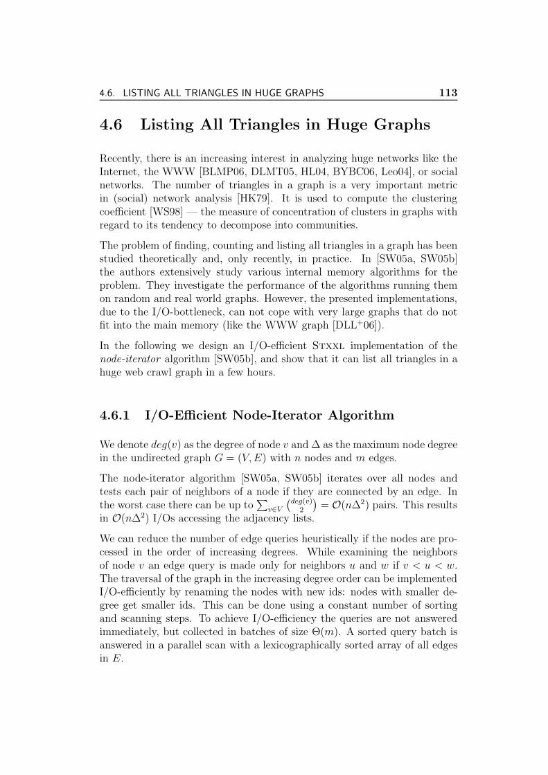
4.6. LISTING ALL TRIANGLES IN HUGE GRAPHS 113
4.6 Listing All Triangles in Huge Graphs
Recently, there is an increasing interest in analyzing huge networks like theInternet, the WWW [BLMP06, DLMT05, HL04, BYBC06, Leo04], or socialnetworks. The number of triangles in a graph is a very important metricin (social) network analysis [HK79]. It is used to compute the clusteringcoefficient [WS98] — the measure of concentration of clusters in graphs withregard to its tendency to decompose into communities.
The problem of finding, counting and listing all triangles in a graph has beenstudied theoretically and, only recently, in practice. In [SW05a, SW05b]the authors extensively study various internal memory algorithms for theproblem. They investigate the performance of the algorithms running themon random and real world graphs. However, the presented implementations,due to the I/O-bottleneck, can not cope with very large graphs that do notfit into the main memory (like the WWW graph [DLL+06]).
In the following we design an I/O-efficient Stxxl implementation of thenode-iterator algorithm [SW05b], and show that it can list all triangles in ahuge web crawl graph in a few hours.
4.6.1 I/O-Efficient Node-Iterator Algorithm
We denote deg(v) as the degree of node v and ∆ as the maximum node degreein the undirected graph G = (V, E) with n nodes and m edges.
The node-iterator algorithm [SW05a, SW05b] iterates over all nodes andtests each pair of neighbors of a node if they are connected by an edge. Inthe worst case there can be up to
∑
v∈V
(
deg(v)2
)
= O(n∆2) pairs. This resultsin O(n∆2) I/Os accessing the adjacency lists.
We can reduce the number of edge queries heuristically if the nodes are pro-cessed in the order of increasing degrees. While examining the neighborsof node v an edge query is made only for neighbors u and w if v < u < w.The traversal of the graph in the increasing degree order can be implementedI/O-efficiently by renaming the nodes with new ids: nodes with smaller de-gree get smaller ids. This can be done using a constant number of sortingand scanning steps. To achieve I/O-efficiency the queries are not answeredimmediately, but collected in batches of size Θ(m). A sorted query batch isanswered in a parallel scan with a lexicographically sorted array of all edgesin E.
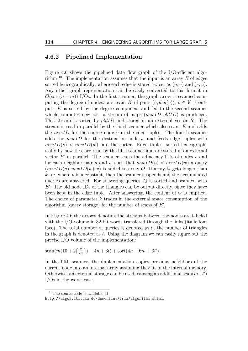
114 CHAPTER 4. ENGINEERING ALGORITHMS FOR LARGE GRAPHS
4.6.2 Pipelined Implementation
Figure 4.6 shows the pipelined data flow graph of the I/O-efficient algo-rithm 10. The implementation assumes that the input is an array E of edgessorted lexicographically, where each edge is stored twice: as (u, v) and (v, u).Any other graph representation can be easily converted to this format inO(sort(n + m)) I/Os. In the first scanner, the graph array is scanned com-puting the degree of nodes: a stream K of pairs (v, deg(v)), v ∈ V is out-put. K is sorted by the degree component and fed to the second scannerwhich computes new ids: a stream of maps (newID, oldID) is produced.This stream is sorted by oldID and stored in an external vector R. Thestream is read in parallel by the third scanner which also scans E and addsthe newID for the source node v in the edge tuples. The fourth scanneradds the newID for the destination node w and feeds edge tuples withnewID(v) < newID(w) into the sorter. Edge tuples, sorted lexicograph-ically by new IDs, are read by the fifth scanner and are stored in an externalvector E ′ in parallel. The scanner scans the adjacency lists of nodes v andfor each neighbor pair u and w such that newID(u) < newID(w) a query(newID(u), newID(w), v) is added to array Q. If array Q gets longer thank ·m, where k is a constant, then the scanner suspends and the accumulatedqueries are answered. For answering queries, Q is sorted and scanned withE ′. The old node IDs of the triangles can be output directly, since they havebeen kept in the edge tuple. After answering, the content of Q is emptied.The choice of parameter k trades in the external space consumption of thealgorithm (query storage) for the number of scans of E ′.
In Figure 4.6 the arrows denoting the streams between the nodes are labeledwith the I/O-volume in 32-bit words transfered through the links (italic fontface). The total number of queries is denoted as t′, the number of trianglesin the graph is denoted as t. Using the diagram we can easily figure out theprecise I/O volume of the implementation:
scan(m(10 + 2⌈ t′
km⌉) + 4n + 3t) + sort(4n + 6m + 3t′).
In the fifth scanner, the implementation copies previous neighbors of thecurrent node into an internal array assuming they fit in the internal memory.Otherwise, an external storage can be used, causing an additional scan(m+t′)I/Os in the worst case.
10The source code is available athttp://algo2.iti.uka.de/dementiev/tria/algorithm.shtml.

4.6. LISTING ALL TRIANGLES IN HUGE GRAPHS 115
t’km
E
sort
sort
sort
sort
T
E’
sortAnswer queries
R
Q
4m
4m
2n
2n2n
2n
4m
2m2m
3t’3t
2m
K
1. compute degrees
2. generate new ids
3. add new ID for src
4. add new ID for dst
5. generate triangle queries
6. answer queries
Figure 4.6: The pipelined scheme of the triangle counting/listing algorithm.
116 CHAPTER 4. ENGINEERING ALGORITHMS FOR LARGE GRAPHS
4.6.3 Experiments
Using our Stxxl implementation we have counted the number of triangles ina web crawl graph from the WebBase project 11. In this graph the nodes areweb pages and the edges are hyperlinks between them. For the computationwe ignored the direction of the links. Our crawl graph had 135 million nodesand 1.2 billion edges. The machine we have used is described in Section 2.4as SCSIOpteron. The difference is that we have used seven hards disks andone GByte of main memory. During the computation which took only 4h46min we have detected 10.6 billion triangles. A total volume of 851 GB wastransferred between the main memory and the hard disks.
11http://www-diglib.stanford.edu/~testbed/doc2/WebBase/
4.7. GRAPH COLORING 117
4.7 Graph Coloring
4.7.1 Introduction
Coloring a graph using as few colors as possible is an important problemhaving many diverse applications, such as solving sparse linear systems ofequations, resource allocation, scheduling, and the construction and testingof VLSI circuits. Finding the smallest possible number of colors is known tobe an NP-complete problem. Therefore it makes more sense to concentrateon fast algorithms that give good non-optimal colorings. A class of suchalgorithms are heuristics, they do not give guarantees on the quality of theproduced coloring, however, they give colorings with a small number of colorson real-world instances and are very fast. Highest-degree-first [WP67] andsmallest-degree-last [MMI72] are the classical heuristics.
A special case of the problem is coloring planar graphs. Finding the mini-mum number of colors for this type of graphs is also NP-complete [GJS76].However, it is known that the nodes of every planar graph can be coloredwith at most four colors. The best known internal memory O(n2) algorithm[RSST96] for finding such a color assignment has very large constants and isconsidered impractical. Coloring planar graphs with five colors can be donefaster, in linear time [Fre84].
The problem of coloring has been studied theoretically and experimentallyin the standard RAM model (see links in [Cul]). Solving the problem ofcoloring in more advanced models of computation has attracted much atten-tion. Many parallel and distributed coloring algorithms have been published,however, much less has been done to evaluate these algorithms experimen-tally. Parallel variants of the highest-degree-first and smallest-degree-lastheuristics are implemented in [ABC+95]. In the paper [JP93] the authorsdevise a heuristic for distributed memory computers that generates color-ings of a quality comparable with sequential greedy heuristics. Finnocchi etal. [FPS05] provides a very detailed experimental study of fast randomizeddistributed memory heuristics.
Many efficient parallel algorithms have been devised for finding a color assign-ment with 8,7,6 and 5 colors [GPS87, Nao87, BK87, HCD89, Dik86, BJ85]for planar graphs. The main idea behind most of these algorithms is to re-move a constant fraction of small degree nodes and proceed with computingthe coloring of the (modified) rest of the graph recursively. Then, the set ofthe removed nodes is colored based on the colors of the remaining nodes.
Parallel algorithms for coloring planar algorithms with only seven colors (7-
118 CHAPTER 4. ENGINEERING ALGORITHMS FOR LARGE GRAPHS
coloring) can be considered folklore. In at least two papers [GPS87, Nao87]the authors propose a simple graph reduction, which leads to an optimal ex-ternal memory coloring algorithms. The reduction allows to remove at least1/6 nodes of the graph keeping it planar. The authors of [Nao87, BK87]came up with somewhat complicated (R)NC parallel algorithms for the 5-color version of the problem. The algorithms run in Ω
(
log3 n)
suboptimalworst-case parallel time and use the computation of connected components asa subroutine. Diks [Dik86] presented a very complicated parallel 6-coloringalgorithm, which requires an efficient BFS algorithm as a subroutine. Thereis an optimal parallel algorithm that can 5-color planar graphs [HCD89]. Itsexternalization can give an I/O-efficient algorithm with sorting time com-plexity. The algorithm is far from being practical: its reduction procedureis very expensive and it can only reduce a tiny number of nodes (< n/196)in a recursion in the worst case. A similar 5-coloring algorithm in [GPS87]reduces the node set in the recursion by an even smaller fraction in the worstcase.
Although parallel (coloring) algorithms can often be reformulated as externalalgorithms, the external memory model gives us additional opportunities. Inparticular, the technique of time forward processing is I/O-efficient yet in-herently sequential. The only coloring algorithm explicitly developed for theI/O model we are aware of is the greedy algorithm by Zeh [Zeh02]. Althoughthis algorithm is based on time forward processing, it can be viewed as aparticularly efficient externalization of the parallel algorithm from [JP93]. Aparticular application of an external memory coloring algorithm would becomputing a schedule for executing many parallel jobs if only a single pro-cessor is available for computing the schedule. Each color gives a subset ofjobs that can be processed in parallel.
Our contributions. We propose a fast I/O-efficient implementation of theHighest-Degree-First graph coloring heuristic, a new external memory vari-ant of the Smallest-Degree-First heuristic, and its implementation, developnew simple I/O-efficient algorithms for computing 6- and 7-colorings of pla-nar graphs, provide a practical implementation of the 7-coloring algorithm,and show how to implement the 2-coloring algorithm I/O-efficiently. Weimplement the algorithms using the Stxxl library and compare the perfor-mance of the devised implementations experimentally, running them on hugerandom and real-world graph instances. To the best of our knowledge, noalgorithm for finding good colorings of graphs exceeding the size of the mainmemory has been published so far. Our experimental study of I/O-efficientcoloring algorithms is the first of that kind.
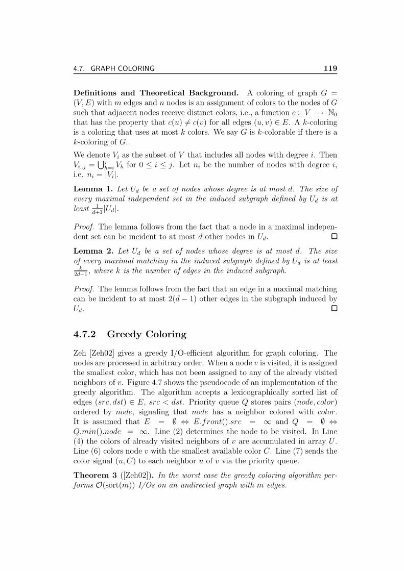
4.7. GRAPH COLORING 119
Definitions and Theoretical Background. A coloring of graph G =(V, E) with m edges and n nodes is an assignment of colors to the nodes of Gsuch that adjacent nodes receive distinct colors, i.e., a function c : V → N0
that has the property that c(u) 6= c(v) for all edges (u, v) ∈ E. A k-coloringis a coloring that uses at most k colors. We say G is k-colorable if there is ak-coloring of G.
We denote Vi as the subset of V that includes all nodes with degree i. ThenVi..j =
⋃jh=i Vh for 0 ≤ i ≤ j. Let ni be the number of nodes with degree i,
i.e. ni = |Vi|.Lemma 1. Let Ud be a set of nodes whose degree is at most d. The size ofevery maximal independent set in the induced subgraph defined by Ud is atleast 1
d+1|Ud|.
Proof. The lemma follows from the fact that a node in a maximal indepen-dent set can be incident to at most d other nodes in Ud.
Lemma 2. Let Ud be a set of nodes whose degree is at most d. The sizeof every maximal matching in the induced subgraph defined by Ud is at least
k2d−1
, where k is the number of edges in the induced subgraph.
Proof. The lemma follows from the fact that an edge in a maximal matchingcan be incident to at most 2(d − 1) other edges in the subgraph induced byUd.
4.7.2 Greedy Coloring
Zeh [Zeh02] gives a greedy I/O-efficient algorithm for graph coloring. Thenodes are processed in arbitrary order. When a node v is visited, it is assignedthe smallest color, which has not been assigned to any of the already visitedneighbors of v. Figure 4.7 shows the pseudocode of an implementation of thegreedy algorithm. The algorithm accepts a lexicographically sorted list ofedges (src, dst) ∈ E, src < dst. Priority queue Q stores pairs (node, color)ordered by node, signaling that node has a neighbor colored with color.It is assumed that E = ∅ ⇔ E.front().src = ∞ and Q = ∅ ⇔Q.min().node = ∞. Line (2) determines the node to be visited. In Line(4) the colors of already visited neighbors of v are accumulated in array U .Line (6) colors node v with the smallest available color C. Line (7) sends thecolor signal (u, C) to each neighbor u of v via the priority queue.
Theorem 3 ([Zeh02]). In the worst case the greedy coloring algorithm per-forms O(sort(m)) I/Os on an undirected graph with m edges.

120 CHAPTER 4. ENGINEERING ALGORITHMS FOR LARGE GRAPHS
Function GreedyColoring(E)ExternalPriorityQueue: Q // stores neighbor colorswhile E 6= ∅ ∨ Q 6= ∅ do (1)
v := minE .front().src,Q .min().node (2)U := ∅ //used colors (3)while v = Q .min().node do U .append(Q .delMin().color) od (4)sort U (5)scan U and assign node v color C := minc 6∈U c (6)while v = E .front().src do Q .insert((E .popFront().dst ,C )) od (7)
Figure 4.7: The implementation of the greedy algorithm.
Proof. The algorithm performs m insertions in the priority queue, each taking(1/B) logM/B(m/M) amortized I/Os [San00]. Sorting and scanning in Lines(5–6) take
∑
v∈V sort(deg(v)) + scan(deg(v)) ≤ sort(2m) + scan(2m) I/Os.For each visited node v, there is a color in [0, . . . , d] which has not beenassigned to a neighbor of v. Therefore, at most d + 1 colors are used.
4.7.3 Highest-Degree-First Heuristic
HDF heuristic is a variant of the greedy algorithm that visits and colors thenodes in the order of their degree, starting from highest degree nodes. A highlevel pseudocode of the I/O-efficient HDF heuristic is shown in Figure 4.8.The algorithm accepts a lexicographically sorted list of edges (src, dst) ∈ E,src < dst.
(1) Rename nodes in E such thatdeg(v) > deg(u) ⇒ newName(v) < newName(u).
(2) Call GreedyColoring(E ) computing a coloring.
(3) Restore the old names in the coloring.
Figure 4.8: The I/O-efficient HDF algorithm.
Corollary 4. The I/O-efficient HDF heuristic colors an undirected graphwith m edges in O(sort(m)) I/Os.
4.7. GRAPH COLORING 121
The pipelined scheme of our Stxxl HDF heuristic implementation is pre-sented in Figure 4.9. Renaming of the nodes according to their degree isimplemented using a constant number of scan/sort passes in blocks from (a)to (k). Calling greedy coloring in block (l) colors the graph with new nodeids. The old ids are restored in blocks (m)–(n).
Now we treat the diagram in detail. The algorithm duplicates each in-coming each edge producing two edges: (u, v) and (v, u) for (u, v) ∈ E(a). While processing (b) the sorted adjacency lists, stream of pairs J =(v, deg(v)) : v ∈ V is computed (c). Stream J is sorted by deg(v) in de-scending order (d). The nodes are numbered in (e): node v obtains a newID that is equal to the position of pair (v, d) in the sorted stream J ; pair(v, newID) is output; v is appended to external array O. The name maps(oldID, newID) are sorted in (f) and stored in external array R. Blocks(g)–(i) rename the nodes in edges E. Block (j) exchanges src and dst inedges with src > dst. Edges ordered by src are fed to the greedy coloringalgorithm (l). The nodes in the result of (l) receive their old names in (m).
We can precisely compute the worst case I/O volume of the implementationconsidering the data flow between the nodes in the diagram. Assuming thatthe pipelined sorters need only one merge pass and with proper settings thepriority queue performs only (64m/DB) I/Os [San00], and node and colorids are represented with 4-byte C++ ints, then the pipelined HDF heuristichas I/O volume at most 112m+72n bytes. A non-pipelined implementationwould transfer 224m + 120n bytes.
4.7.4 Batched Smallest-Degree-Last Heuristic
The Smallest-Degree-Last (SDL) heuristic [MMI72] algorithm operates intwo phases. In the first phase, it removes a node with smallest degree fromthe graph (reducing the degrees of its neighbors). The procedure is appliedrecursively to the graph that remains. Denote the node removed in recursioni as vi. The second phase of the algorithm greedily colors the nodes of thegraph in the backward order vn,vn−1,. . .,v1.
A direct implementation of the SDL heuristic needs to do random accessesto the adjacency lists of vi and its neighbors in each recursion, thereforethe implementation might require Ω (m) I/Os. We propose the BatchedSmallest-Degree-Last heuristic (BSDL), where a set of small degree nodes(batch) is removed in a recursion. The recursion step gets more expen-sive with respect to the number of I/Os and internal work, but the totalnumber of recursions is reduced. Nodes with degrees at most δ(V, E) are

122 CHAPTER 4. ENGINEERING ALGORITHMS FOR LARGE GRAPHS
sort by src node (b)
duplicate (a)
(c)compute degrees
E
sort by degree (d)
number nodes (e)
(f)
sort by dst node (h)
sort by oldID
src−>newID(src) (g)
R
(i)dst−>newID(dst)
OGreedyColoring
sort by src node
orient (j)
(k)
(l)
(n)sort by node
E’
E’
result
(node,color)
J
(oldID,newID)
(oldID)
node−>oldID(node) (m)
Figure 4.9: The pipelined scheme of the I/O-efficient HDF algorithm.
4.7. GRAPH COLORING 123
taken in a batch, where function δ maps a graph to an integer in the range[minv∈V deg(v) ,∞). We will refer to function δ as the maximum batchdegree function. The choice of this function balances the quality of the col-oring and the running time of the heuristic: the smaller the value of δ(V, E),the fewer color classes are used, and the slower the graph is reduced. Ideally,the computation of the value of δ(V, E) should not cause much computa-tional and I/O overhead. In this thesis, we experimentally investigate anobvious maximum batch degree function: the rounded up average degreeδ(V, E) = ⌈2|E|/|V |⌉. Other possible functions one might consider are themedian degree, node c-quantile δ(V, E) = min k : |V1..k| ≥ cn, edge c-quantile δ(V, E) = min
k :∑
v∈V1..kdeg(v) ≥ 2mc
. However, the values ofthose functions are more expensive to compute.
The I/O-efficient BSDL procedure is shown in Figure 4.10.
(1) Compute the value of δ(V, E).
(2) Find the set of nodes R = v : v ∈ V, deg(v) ≤ δ(V, E).
(3) Delete the nodes in R from the graph G reducing it to graph G′ =(V ′, E ′), where V ′ = V − R and E ′ = (u, v) ∈ E | u, v ∈ V ′.
(4) Color G′ recursively.
(5) Color the nodes in R calling GreedyColoring on the subgraph of Ginduced by R. Before running the algorithm the priority queue isfilled with entries signaling the existence of already colored neighborsof nodes in R, i.e. values (v, color(u)) | (u, v) ∈ E, v ∈ R, u 6∈ R areinserted.
Figure 4.10: I/O-efficient implementation of the Batched Smallest-Degree-Last coloring heuristic.
Figure 4.11 depicts an Stxxl pipelined implementation of the recursion ofthe I/O-efficient BSDL heuristic. The nodes to remove R, the edges incidentto R and the input graph G′ for the recursion call are computed in a constantnumber of scan/sort passes in blocks from (a) to (g). After the recursion thenodes in set R are colored using the greedy coloring algorithm and a fewscan/sort passes (blocks (j)–(l)).
Now we consider the processing that goes on in the implementation in detail:In each recursion, the algorithm receives a stream of edges E sorted by thesource node, which is fed into the duplicate algorithm (a). For each incoming

124 CHAPTER 4. ENGINEERING ALGORITHMS FOR LARGE GRAPHS
edge (v, w) the duplicate algorithm outputs two edges (v, w) and (w, v) tothe output stream, which is consumed by the sorter (b). The output of sorteris a sequence of adjacency lists, which is fed to the algorithm (c), computingthe degrees of the nodes. In algorithm (d) the value of function δ(V, E) iscomputed. The stream of triples in the form (src, dst, deg(src)) is analyzed,passing the triples (src, dst, B), src < dst with binary bit B = (deg(src) ≤δ(V, E)) to sorter (e) and pushing the nodes src ∈ R to an external vector.To save I/O volume, field B is coded as the most significant bit of the srcfield. In our implementation, algorithms (c) and (d) are combined into onealgorithm to reduce the computational overhead. Algorithm (f) passes the in-coming edge (src, dst) from sorter (e) to the next recursion (f) if src, dst 6∈ R.Edges in EC = (src, dst) | src, dst ∈ R are fed to sorter (i), and edges inEIN = (dst, src) | src 6∈ R, dst ∈ R ∪ (src, dst) | src ∈ R, dst 6∈ R go tosorter (h). Let V ′
0(i) be the set of nodes v ∈ V ′ having degree zero in graph G′
in the current recursion i, i.e., the nodes that become isolated after removalof edges EIN , and let V ∗
0 =⋃∞
j=i V′0(j). Then the stream of color assignments
(v′, color(v′)), v′ ∈ V ′ − V ∗0 sorted by v′ comes from the recursion call (g).
Algorithm (j) initializes the priority queue used in the GreedyColoring withentries (v, color(u)), v ∈ R, u ∈ V ′, indicating that node v has a neighborcolored with color(u). For nodes u ∈ V ∗
0 algorithm (j) assumes that theyhave color 0. This way the nodes in V ∗
0 are implicitly colored with zeros.Nodes in R are colored calling GreedyColoring on graph (V, EC) (k). Algo-rithm (l) merges the color assignment stream from algorithm (k) with thecolor assignments of nodes in G′ stored in external array C. The array C isrewritten with the output of algorithm (l), such that it finally contains thecolor assignments for all nodes in G − V ∗
0 .
4.7.5 7-Coloring of Planar Graphs
In this section we show that the BSDL heuristic with maximum batch de-gree function δ(V, E) = 6 computes a 7-coloring of a planar graph I/O inO(sort(m)) I/Os. In contrast to the parallel algorithm of Naor [Nao87] our7-coloring algorithm does not filter adjacent nodes computing a maximal in-dependent set of R. Using the time-forward-processing technique we are ableto reduce by more nodes per iteration.
Lemma 5 ([Nao87]). In planar graphs, the number of nodes with a degreeless than seven is at least n/6.

4.7. GRAPH COLORING 125
EC
sort by src node (b)
duplicate (a)
(c)compute degrees
filter edges (d)
E
R
(g)
dst R AND B=0
(f)categorize
sort by dst node (e)
(src,dst,B)
recursion (h)sort by dst node
(j)initialize PQsort by src node (i)
(k)GreedyColoring
update colors C
(v,color(v))
(l)
dst R AND B=1
(dst R AND B=0)
(dst R AND B=1)OR
E IN
Figure 4.11: The pipelined scheme of the Batched Smallest-Degree-Last col-oring heuristic.
126 CHAPTER 4. ENGINEERING ALGORITHMS FOR LARGE GRAPHS
Proof. According to Euler’s formula for planar graphs [Har69]:
2m < 6n (4.1)
or
∞∑
i=1
i ni < 6
∞∑
i=1
ni
We have∑∞
i=1 i ni =∑6
i=1 i ni +∑∞
i=7 i ni ≥∑6
i=1 ni + 7∑∞
i=7 ni. On theother hand 6
∑∞i=1 ni = 6
∑6i=1 ni + 6
∑∞i=7 ni. Then
∑6i=1 ni + 7
∑∞i=7 ni <
6∑6
i=1 ni + 6∑∞
i=7 ni. Subtracting 6∑∞
i=7 ni on both sides we get∑6
i=1 ni +∑∞
i=7 ni < 6∑6
i=1 ni ⇔ n < 6∑6
i=1 ni.
Theorem 6. The BSDL heuristic with maximum batch degree functionδ(V, E) = 6 computes a 7-coloring of a planar graph in O(sort(m)) I/Os.
Proof. The pipelined implementation implies that steps (1)–(3) run inO(sort(m)) I/Os. Step (5) needs O(sort(m)) I/Os by Theorem 3. Lemma 5states that |R| ≥ n
6, then by Euler’s formula (Equation 4.1): |R| > m
18. Since
every node in R has at least one edge, the edge set E ′ has at most a constantfraction of edges in E: |E ′| < 17
18m. Therefore the I/O complexity of the
algorithm can be expressed as:
T (m) < O(sort(m)) + T
(
17
18m
)
The recurrence has the solution T (m) = O(sort(m)).
Since the maximum degree of nodes R in graph (V, EC ∪ EIN) is at most6, then by Theorem 3 the number of colors used by the heuristic is at most7.
Analyzing the data flow between and inside the blocks in the diagram shownin Figure 4.11, we can obtain the worst case I/O volume of the 7-coloringalgorithm. With the same assumptions about the I/O volume of the pipelinedsorters and priority queue as in Section 4.7.3, the I/O volume of the 7-coloringalgorithm is 1168m + 144n bytes in the worst case. Without pipelining itwould be 3192m + 336n bytes.

4.7. GRAPH COLORING 127
4.7.6 6-Coloring of Planar Graphs
In this section, we present an I/O-efficient algorithm that 6-colors planargraphs. As in the 7-coloring algorithm we try to find a set of low degreenodes R whose size is at least a constant fraction of the total number of nodes.This set contains the candidates for removal. In our 6-coloring algorithm, incontrast to 7-coloring, not all nodes with degree six are taken into R, onetakes only those having at least two neighbors that can be merged into onenode efficiently, thus reducing the maximum possible number of neighborcolors to five. In candidate set R we include two categories of nodes:
(1) nodes with a degree at most five, V1..5.
(2) nodes with degree six having at most two large neighbors. We denotethis set as V ′
6 ⊆ V6, and the cardinality of this set we denote as n′6.
Lemma 7 proves that there is a sufficient number of nodes of that kind.Amazingly, the worst case ratio between the size of the candidate set R andn is the same as in the 7-coloring algorithm (Lemma 5), i.e. the number ofdegree-six nodes rejected in condition (2) is small.
Definition: A node is small if it has at most K neighbors, large otherwise.deg(v) denotes the degree of node v.
Lemma 7. There exists a constant K such that the number of nodes in setR is at least n/6.
Proof. First let us bound the number of nodes with degree six having at leastthree large neighbors (n6−n′
6). Consider the worst case when the large nodesare incident only to the degree-six nodes. Moreover, each node of degree sixhas exactly three edges connecting it to the large degree nodes. Then:
n6 − n′6 ≤
∑∞i=K+1 i ni
3
or
3n′6 ≥ 3n6 −
∞∑
i=K+1
i ni (4.2)
128 CHAPTER 4. ENGINEERING ALGORITHMS FOR LARGE GRAPHS
According to Euler’s formula
2m < 6n
⇒∞
∑
i=1
i ni < 6∞
∑
i=1
ni
⇒5
∑
i=1
i ni + 6n6 +
∞∑
i=7
i ni < 6
5∑
i=1
ni + 6n6 + 6
∞∑
i=7
ni
⇒∞
∑
i=7
(i − 6)ni +
5∑
i=1
i ni − 6
5∑
i=1
ni < 0
⇒∞
∑
i=7
(i − 6)ni +5
∑
i=1
ni − 65
∑
i=1
ni < 0
⇒ 0 >
∞∑
i=7
(i − 6)ni − 5
5∑
i=1
ni (4.3)
We add α times Inequality (4.3) to Inequality (4.2):
3n′6 > 3n6 + α
∞∑
i=7
(i − 6)ni −∞
∑
i=K+1
i ni − 5α
5∑
i=1
ni
⇒ 5α
5∑
i=1
ni + 3n′6 > 3n6 + α
K∑
i=7
(i − 6)ni +
∞∑
i=K+1
((α − 1)i − 6α)ni
⇒ 5α5
∑
i=1
ni + 3n′6 > 3n6 + α
K∑
i=7
ni +∞
∑
i=K+1
((α − 1)(K + 1) − 6α)ni
For all K ≥ 10 the ratio 5αmin3,α,(α−1)(K+1)−6α
is minimal with α = 3. Plug-ging in the values of α and K = 10 we obtain:
4.7. GRAPH COLORING 129
155
∑
i=1
ni + 3n′6 > 3n6 + 3
K∑
i=7
ni + 4∞
∑
i=K+1
ni
⇒ 155
∑
i=1
ni + 3n′6 > 3
∞∑
i=6
ni
⇒ 5
5∑
i=1
ni + n′6 >
∞∑
i=6
ni
Adding∑5
i=1 ni to both sides of the inequality we arrive at:
65
∑
i=1
ni + n′6 >
∞∑
i=1
ni
Finally:
6(
5∑
i=1
ni + n′6) >
∞∑
i=1
ni = n
⇒ |R| >n
6
The algorithms for 5-coloring planar graphs in [HCD89, GPS87] have similarconstructions of candidate sets. However, they guarantee only a very smallratios |R|/n (1/196 and 1/301 accordingly), which may lead to huge con-stants in the overall running times. Our construction is more practical: thereduction step is simpler and it can find more nodes in the worst case.
Now we present the algorithmical procedure of the reduction step. Let R′
be a maximal independent set of R. The nodes in R′ having a degree lessthan six (V1..5∩R′) are deleted from the graph as in the 7-coloring algorithm.We delete every node in V ′
6 ∩ R′ from G and merge two non-adjacent smallneighbors in a single node concatenating their adjacency lists. Such two nodesalways exist, since otherwise there is a clique on five nodes (the degree-six
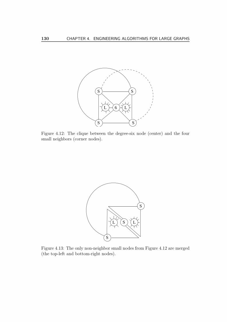
130 CHAPTER 4. ENGINEERING ALGORITHMS FOR LARGE GRAPHS
S
SS
6
S
L L
Figure 4.12: The clique between the degree-six node (center) and the foursmall neighbors (corner nodes).
S
S
L LS
Figure 4.13: The only non-neighbor small nodes from Figure 4.12 are merged(the top-left and bottom-right nodes).
4.7. GRAPH COLORING 131
node and its four small neighbors, see Figure 4.12). It is easy to see thatafter the described reduction, the graph remains planar (see Figure 4.13).
In general, two or more nodes in V ′6 can cause the merging of the same node:
v1 ∈ V ′6 merges node w1 with w2 and v2 ∈ V ′
6 merges node w1 with w3. Toresolve these conflicts we propose two solutions. The first approach com-putes the connected components in graph Gc with a node set Vc consisting ofnodes that have to be merged and the edge set Ec, which models the mergeoperations: edge (w1, w2) is in Ec if w1 has to be merged with w2. Then wecompute the connected components of the planar graph Gc, using the algo-rithm in [CGG+95] in O(sort(n)) I/Os. Each connected component includesthe set of nodes that have to be merged together in one node. The mergingis then done by renaming the nodes to the node id of the representative nodeof the respective connected component. This can be performed in a constantnumber of sort and scan operations.
Our second solution does not require calling the connected components sub-procedure. We compute a maximal matching Mc of the (multi)graph Gc
using a simple algorithm from [Zeh02] running in O(sort(n)) I/Os. We per-form only those merge operations that are present in Mc. We also have toremove the nodes from R′ which contributed to Gc, but their merge opera-tions were filtered out from Mc. Since all nodes in Gc are small, this can beimplemented using O(sort(n)) I/Os. The degree of a node v ∈ Gc can be atmost K, since for each edge (v, u) ∈ E, u ∈ V ′
6 ∩R′, there is exactly one edge(v, w) ∈ Gc and node v is small in G. Therefore by Lemma 2 set R′ mightbe reduced in size by a factor at most 1/(2K − 1).
It is not clear which solution is faster: connected components is a moreexpensive procedure in the external memory, but the approach does notreduce set R′; the second solution is cheaper but might reduce set R′ byfactor 1/(2K−1) in the worst case, i. e. postponing the computation to laterrecursions.
Summing all up we present a high-level scheme of the algorithm in Figure 4.14
Theorem 8. The I/O-efficient algorithm for computing 6-coloring of a pla-nar graph runs in O(sort(m)) I/Os.
Proof. Steps (1)–(5) and (7)–(8) can be implemented in a constant numberof sort and scan steps. From Lemma 7, Lemma 1 and Lemma 2 it follows
that |V ′| ≤(
1 − 16·7·(2K−1)
)
n. Then, by the Euler’s formula (Equation 4.1)
there exists a constant q, such that |E ′| ≤ q · m, 0 ≤ q < 1. Hence the I/Ocomplexity of the algorithm can be expressed as:
T (m) ≤ O(sort(m)) + T (q · m)
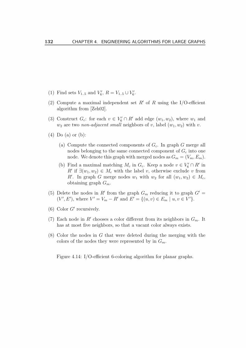
132 CHAPTER 4. ENGINEERING ALGORITHMS FOR LARGE GRAPHS
(1) Find sets V1..5 and V ′6 , R = V1..5 ∪ V ′
6 .
(2) Compute a maximal independent set R′ of R using the I/O-efficientalgorithm from [Zeh02].
(3) Construct Gc: for each v ∈ V ′6 ∩ R′ add edge (w1, w2), where w1 and
w2 are two non-adjacent small neighbors of v, label (w1, w2) with v.
(4) Do (a) or (b):
(a) Compute the connected components of Gc. In graph G merge allnodes belonging to the same connected component of Gc into onenode. We denote this graph with merged nodes as Gm = (Vm, Em).
(b) Find a maximal matching Mc in Gc. Keep a node v ∈ V ′6 ∩ R′ in
R′ if ∃(w1, w2) ∈ Mc with the label v, otherwise exclude v fromR′. In graph G merge nodes w1 with w2 for all (w1, w2) ∈ Mc,obtaining graph Gm.
(5) Delete the nodes in R′ from the graph Gm reducing it to graph G′ =(V ′, E ′), where V ′ = Vm − R′ and E ′ = (u, v) ∈ Em | u, v ∈ V ′.
(6) Color G′ recursively.
(7) Each node in R′ chooses a color different from its neighbors in Gm. Ithas at most five neighbors, so that a vacant color always exists.
(8) Color the nodes in G that were deleted during the merging with thecolors of the nodes they were represented by in Gm.
Figure 4.14: I/O-efficient 6-coloring algorithm for planar graphs.
4.7. GRAPH COLORING 133
The recurrence is solved by T (m) = O(sort(m)).
4.7.7 2-Coloring
The well known linear time algorithm for finding a 2-coloring of agraph (or proving that no 2-coloring exists)12 can be implemented I/O-efficiently. The algorithm computes a spanning forest of the graph inO(sort(m)(1 + log log(B · n/m))) I/Os using the deterministic algorithm[MR99] or in O(sort(m)) I/Os using the randomized algorithm [ABW02].Around each tree of the spanning forest, an Euler tour [CGG+95] is computedusing a constant number of sort and scan steps. When the algorithm tra-verses the Euler tours using list ranking [CGG+95], the color (d(v) mod 2)is assigned to node v, where d(v) is a tree distance from the root of nodev. Then, the edge list is scanned: if there is an edge (u, v) ∈ E such thatcolors of u and v match, then the graph has an odd-length cycle and is not2-colorable. Otherwise, the obtained coloring is valid.
Theorem 9. A graph can be 2-colored in O(sort(m)(1 + log log(B · n/m)))I/Os deterministically or in O(sort(m)) expected I/Os.
4.7.8 Experiments
In this section, we experimentally evaluate the performance of the Stxxl
external memory implementations of the HDF heuristic, the BSDL heuristicwith δ(V, E) = ⌈2|E|/|V |⌉, the 7-coloring algorithm for planar graphs (EM7),a tuned SDL implementation from the Boost library (www.boost.org) andan implementation of a 7-coloring algorithm for planar graphs that uses theLEDA library version 5.1 [MN99] (IM7 algorithm) 13. The Boost SDL imple-mentation uses the adjacency list graph representation with std::vectorsstoring the set of vertices and the adjacency structure. This choice reducesthe internal memory consumption and guarantees constant time operationsfor the SDL algorithm. The implementation itself does not modify the inputgraph during the node removal, instead, it maintains an auxiliary array withthe current node degrees. Finding the smallest degree node is implementedwith a bucket priority queue. The IM7 implementation follows the algo-rithm from Figure 4.10 using data type leda::graph to represent graphs.
122-colorability is equivalent to the bipartiteness test.13The source code of the implementations and random graph generators is available at
http://algo2.iti.uka.de/dementiev/files/coloring.tgz.
134 CHAPTER 4. ENGINEERING ALGORITHMS FOR LARGE GRAPHS
Node and edge removal have been implemented via hiding, using the methodleda::graph::hide node.
In the experimental evaluation we have run the implementations on randomand real graph instances:
• G(n, m)-random graphs where edges are generated picking the endpoints uniformly at random from [0, n). Self-loops has been discarded.
• a web crawl graph from the WebBase project14. In this graph the nodesare web pages and edges are hyperlinks between them (the directionwas ignored).
• maximal random planar graphs with m ≈ 3n, which were obtained us-ing the leda::maximal planar map function, and more sparse planargraphs with m = 2n generated by the leda::random planar map func-tion. We could not generate graphs with more than 223 nodes becauseof the 4 GBytes limit of the address space.
• instances of Delaunay triangulations of real-world point sets (NeuseRiver Basin of North Carolina) obtained in [AAY05].
In our experiments we have used three systems running Linux SUSE 9.3 or10.0, their configurations are described in Tables 4.5 and 4.6. The Opteronmachines correspond to the systems described in Section 2.4. The STREAMvalue is the average of the copy, scale, add, and triad memory bandwidthsobtained by the popular STREAM benchmark [Str]. Our programs werecompiled with the GNU C++ compiler version 3.4 and 4.0 with options -O3-DNDEBUG -DLEDA CHECKING OFF. For experiments with external memory im-plementations, we used up to 660 MBytes of the available main memory andblock sizes 512 KBytes or 1 MByte, if not stated otherwise. During all ex-periments, the swap file was switched off to avoid paging. The values of therunning time and the number of used colors for (general and planar) randomgraphs are averaged over runs with 20 random instances.
Figure 4.15 compares the performance of the SDL, BSDL and HDF heuristicson random graphs with a fixed edge probability p = 0.2 15. The smallerinstances fit into the internal memory, for n ≥ 215 the inputs need to beprocessed in external memory. With respect to the running time, the internalmemory SDL shows to be up to 1.6 times faster than the external memory
14http://www-diglib.stanford.edu/~testbed/doc2/WebBase/15We consider all possible edges in an undirected graph with n nodes and choose each
edge with probability p. This is another method to generate G(n, m)-random graphs.
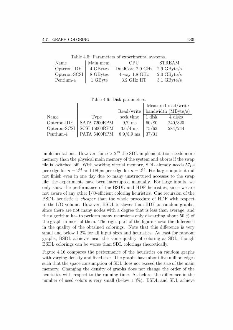
4.7. GRAPH COLORING 135
Table 4.5: Parameters of experimental systems.
Name Main mem. CPU STREAMOpteron-IDE 4 GBytes DualCore 2.0 GHz 2.9 GByte/sOpteron-SCSI 8 GBytes 4-way 1.8 GHz 2.0 GByte/sPentium-4 1 GByte 3.2 GHz HT 3.1 GByte/s
Table 4.6: Disk parameters.
Measured read/writeRead/write bandwidth (MByte/s)
Name Type seek time 1 disk 4 disksOpteron-IDE SATA 7200RPM 9/9 ms 60/80 240/320Opteron-SCSI SCSI 15000RPM 3.6/4 ms 75/63 284/244Pentium-4 PATA 5400RPM 8.9/8.9 ms 37/31
implementations. However, for n > 213 the SDL implementation needs morememory than the physical main memory of the system and aborts if the swapfile is switched off. With working virtual memory, SDL already needs 57µsper edge for n = 214 and 180µs per edge for n = 215. For larger inputs it didnot finish even in one day due to many unstructured accesses to the swapfile; the experiments have been interrupted manually. For large inputs, weonly show the performance of the BSDL and HDF heuristics, since we arenot aware of any other I/O-efficient coloring heuristics. One recursion of theBSDL heuristic is cheaper than the whole procedure of HDF with respectto the I/O volume. However, BSDL is slower than HDF on random graphs,since there are not many nodes with a degree that is less than average, andthe algorithm has to perform many recursions only discarding about 50 % ofthe graph in most of them. The right part of the figure shows the differencein the quality of the obtained colorings. Note that this difference is verysmall and below 1.2% for all input sizes and heuristics. At least for randomgraphs, BSDL achieves near the same quality of coloring as SDL, thoughBSDL colorings can be worse than SDL colorings theoretically.
Figure 4.16 compares the performance of the heuristics on random graphswith varying density and fixed size. The graphs have about five million edgessuch that the space consumption of SDL does not exceed the size of the mainmemory. Changing the density of graphs does not change the order of theheuristics with respect to the running time. As before, the difference in thenumber of used colors is very small (below 1.3%). BSDL and SDL achieve
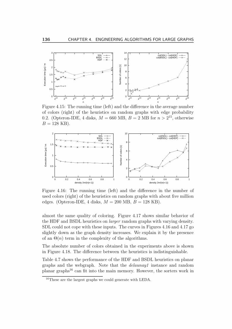
136 CHAPTER 4. ENGINEERING ALGORITHMS FOR LARGE GRAPHS
0
0.5
1
1.5
2
2.5
3
218219216215214213212
Exe
cutio
n tim
e [µ
s] /
m
n
SDLBSDL
HDF
0
2
4
6
8
10
12
14
218219216215214213212
Num
ber
of c
olor
s [1
]
n
col(SDL) - col(HDF)col(BSDL) - col(HDF)
Figure 4.15: The running time (left) and the difference in the average numberof colors (right) of the heuristics on random graphs with edge probability0.2. (Opteron-IDE, 4 disks, M = 660 MB, B = 2 MB for n > 215, otherwiseB = 128 KB).
0
0.5
1
1.5
2
0 0.2 0.4 0.6 0.8 1
Exe
cutio
n tim
e [µ
s] /
m
density 2m/(n(n-1))
SDLBSDL
HDF
0
2
4
6
8
10
0 0.2 0.4 0.6 0.8 1
Num
ber
of c
olor
s [1
]
density 2m/(n(n-1))
col(SDL) - col(HDF)col(BSDL) - col(HDF)
Figure 4.16: The running time (left) and the difference in the number ofused colors (right) of the heuristics on random graphs with about five millionedges. (Opteron-IDE, 4 disks, M = 200 MB, B = 128 KB).
almost the same quality of coloring. Figure 4.17 shows similar behavior ofthe HDF and BSDL heuristics on larger random graphs with varying density.SDL could not cope with these inputs. The curves in Figures 4.16 and 4.17 goslightly down as the graph density increases. We explain it by the presenceof an Θ(n) term in the complexity of the algorithms.
The absolute number of colors obtained in the experiments above is shownin Figure 4.18. The difference between the heuristics is indistinguishable.
Table 4.7 shows the performance of the HDF and BSDL heuristics on planargraphs and the webgraph. Note that the delaunay1 instance and randomplanar graphs16 can fit into the main memory. However, the sorters work in
16These are the largest graphs we could generate with LEDA.
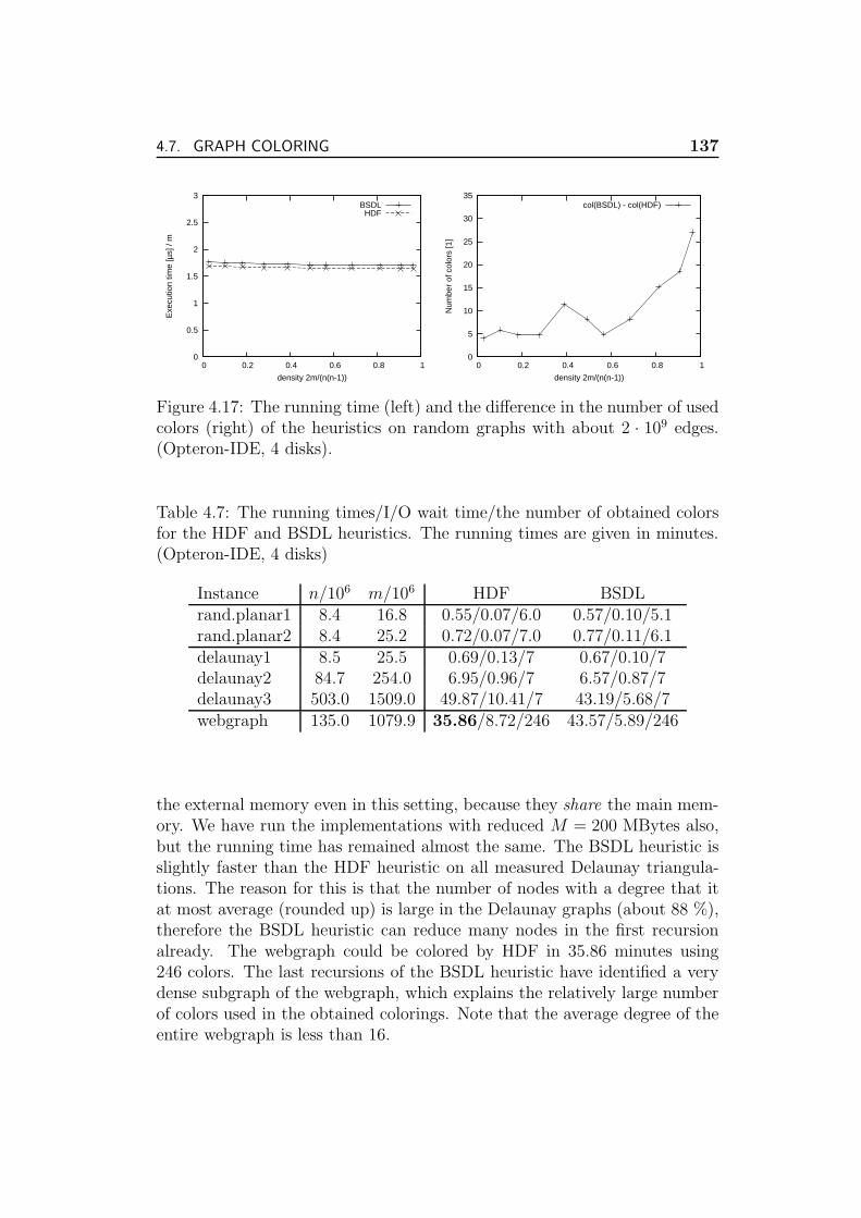
4.7. GRAPH COLORING 137
0
0.5
1
1.5
2
2.5
3
0 0.2 0.4 0.6 0.8 1
Exe
cutio
n tim
e [µ
s] /
m
density 2m/(n(n-1))
BSDLHDF
0
5
10
15
20
25
30
35
0 0.2 0.4 0.6 0.8 1
Num
ber
of c
olor
s [1
]
density 2m/(n(n-1))
col(BSDL) - col(HDF)
Figure 4.17: The running time (left) and the difference in the number of usedcolors (right) of the heuristics on random graphs with about 2 · 109 edges.(Opteron-IDE, 4 disks).
Table 4.7: The running times/I/O wait time/the number of obtained colorsfor the HDF and BSDL heuristics. The running times are given in minutes.(Opteron-IDE, 4 disks)
Instance n/106 m/106 HDF BSDLrand.planar1 8.4 16.8 0.55/0.07/6.0 0.57/0.10/5.1rand.planar2 8.4 25.2 0.72/0.07/7.0 0.77/0.11/6.1delaunay1 8.5 25.5 0.69/0.13/7 0.67/0.10/7delaunay2 84.7 254.0 6.95/0.96/7 6.57/0.87/7delaunay3 503.0 1509.0 49.87/10.41/7 43.19/5.68/7webgraph 135.0 1079.9 35.86/8.72/246 43.57/5.89/246
the external memory even in this setting, because they share the main mem-ory. We have run the implementations with reduced M = 200 MBytes also,but the running time has remained almost the same. The BSDL heuristic isslightly faster than the HDF heuristic on all measured Delaunay triangula-tions. The reason for this is that the number of nodes with a degree that itat most average (rounded up) is large in the Delaunay graphs (about 88 %),therefore the BSDL heuristic can reduce many nodes in the first recursionalready. The webgraph could be colored by HDF in 35.86 minutes using246 colors. The last recursions of the BSDL heuristic have identified a verydense subgraph of the webgraph, which explains the relatively large numberof colors used in the obtained colorings. Note that the average degree of theentire webgraph is less than 16.

138 CHAPTER 4. ENGINEERING ALGORITHMS FOR LARGE GRAPHS
100
1000
10000
218219216215214213212
Num
ber
of c
olor
s [1
]
n
constant edge probability
SDLBSDL
HDF
100
1000
0 0.2 0.4 0.6 0.8 1
Num
ber
of c
olor
s [1
]
density 2m/(n(n-1))
random graphs with about 5 mln edges
SDLBSDL
HDF
1000
10000
0 0.2 0.4 0.6 0.8 1
Num
ber
of c
olor
s [1
]
density 2m/(n(n-1))
random graphs with about 2 109 edges$
BSDLHDF
Figure 4.18: The absolute number of colors obtained by the heuristics onrandom graphs with constant edge probability 0.2, on random graphs withabout five million edges and about 2 · 109 edges.
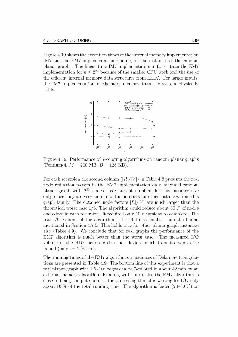
4.7. GRAPH COLORING 139
Figure 4.19 shows the execution times of the internal memory implementationIM7 and the EM7 implementation running on the instances of the randomplanar graphs. The linear time IM7 implementation is faster than the EM7implementation for n ≤ 222 because of the smaller CPU work and the use ofthe efficient internal memory data structures from LEDA. For larger inputs,the IM7 implementation needs more memory than the system physicallyholds.
5
10
15
20
223222221220219218
Exe
cutio
n tim
e [µ
s] /
n
n
EM 7-coloring max.EM 7-coloring m=2n
IM 7-coloring max.IM 7-coloring m=2n
Figure 4.19: Performance of 7-coloring algorithms on random planar graphs(Pentium-4, M = 200 MB, B = 128 KB).
For each recursion the second column (|R|/|V |) in Table 4.8 presents the realnode reduction factors in the EM7 implementation on a maximal randomplanar graph with 223 nodes. We present numbers for this instance sizeonly, since they are very similar to the numbers for other instances from thisgraph family. The obtained node factors |R|/|V | are much larger than thetheoretical worst case 1/6. The algorithm could reduce about 80 % of nodesand edges in each recursion. It required only 10 recursions to complete. Thereal I/O volume of the algorithm is 11–14 times smaller than the boundmentioned in Section 4.7.5. This holds true for other planar graph instancesalso (Table 4.9). We conclude that for real graphs the performance of theEM7 algorithm is much better than the worst case. The measured I/Ovolume of the HDF heuristic does not deviate much from its worst casebound (only 7–15 % less).
The running times of the EM7 algorithm on instances of Delaunay triangula-tions are presented in Table 4.9. The bottom line of this experiment is that areal planar graph with 1.5 · 109 edges can be 7-colored in about 42 min by anexternal memory algorithm. Running with four disks, the EM7 algorithm isclose to being compute-bound: the processing thread is waiting for I/O onlyabout 10 % of the total running time. The algorithm is faster (20–30 %) on
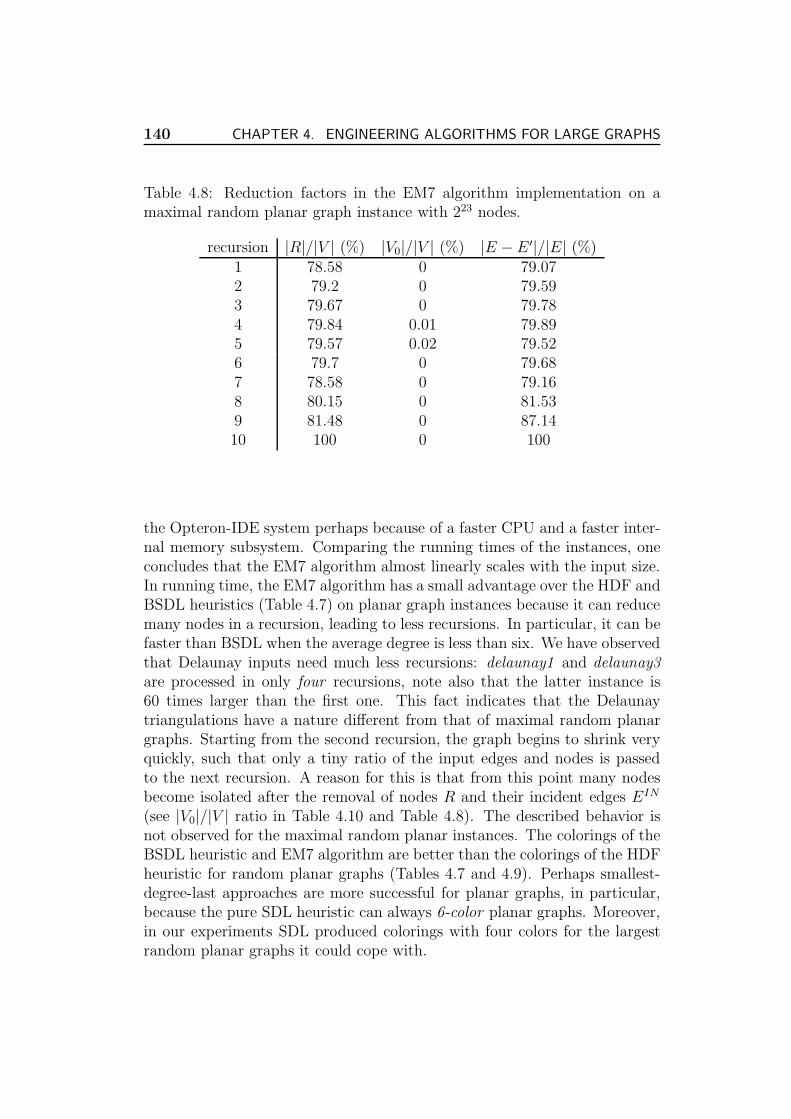
140 CHAPTER 4. ENGINEERING ALGORITHMS FOR LARGE GRAPHS
Table 4.8: Reduction factors in the EM7 algorithm implementation on amaximal random planar graph instance with 223 nodes.
recursion |R|/|V | (%) |V0|/|V | (%) |E − E ′|/|E| (%)1 78.58 0 79.072 79.2 0 79.593 79.67 0 79.784 79.84 0.01 79.895 79.57 0.02 79.526 79.7 0 79.687 78.58 0 79.168 80.15 0 81.539 81.48 0 87.1410 100 0 100
the Opteron-IDE system perhaps because of a faster CPU and a faster inter-nal memory subsystem. Comparing the running times of the instances, oneconcludes that the EM7 algorithm almost linearly scales with the input size.In running time, the EM7 algorithm has a small advantage over the HDF andBSDL heuristics (Table 4.7) on planar graph instances because it can reducemany nodes in a recursion, leading to less recursions. In particular, it can befaster than BSDL when the average degree is less than six. We have observedthat Delaunay inputs need much less recursions: delaunay1 and delaunay3are processed in only four recursions, note also that the latter instance is60 times larger than the first one. This fact indicates that the Delaunaytriangulations have a nature different from that of maximal random planargraphs. Starting from the second recursion, the graph begins to shrink veryquickly, such that only a tiny ratio of the input edges and nodes is passedto the next recursion. A reason for this is that from this point many nodesbecome isolated after the removal of nodes R and their incident edges EIN
(see |V0|/|V | ratio in Table 4.10 and Table 4.8). The described behavior isnot observed for the maximal random planar instances. The colorings of theBSDL heuristic and EM7 algorithm are better than the colorings of the HDFheuristic for random planar graphs (Tables 4.7 and 4.9). Perhaps smallest-degree-last approaches are more successful for planar graphs, in particular,because the pure SDL heuristic can always 6-color planar graphs. Moreover,in our experiments SDL produced colorings with four colors for the largestrandom planar graphs it could cope with.
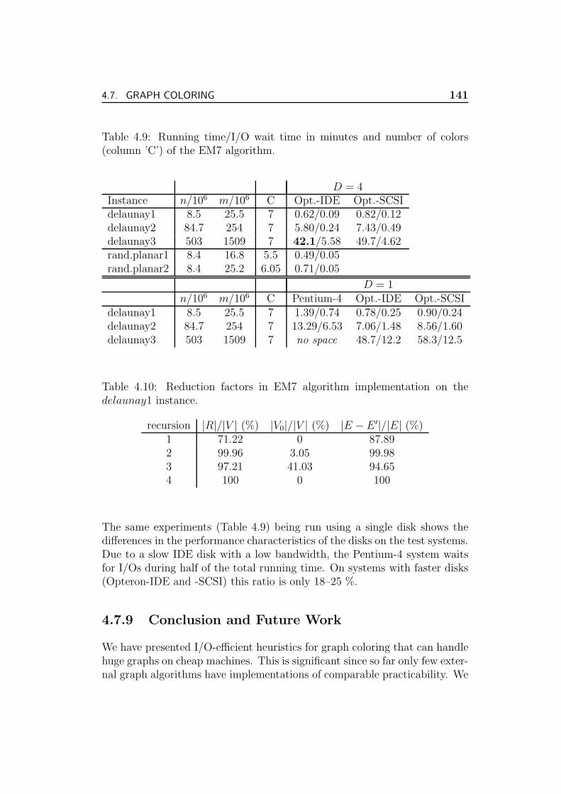
4.7. GRAPH COLORING 141
Table 4.9: Running time/I/O wait time in minutes and number of colors(column ’C’) of the EM7 algorithm.
D = 4Instance n/106 m/106 C Opt.-IDE Opt.-SCSIdelaunay1 8.5 25.5 7 0.62/0.09 0.82/0.12delaunay2 84.7 254 7 5.80/0.24 7.43/0.49delaunay3 503 1509 7 42.1/5.58 49.7/4.62rand.planar1 8.4 16.8 5.5 0.49/0.05rand.planar2 8.4 25.2 6.05 0.71/0.05
D = 1n/106 m/106 C Pentium-4 Opt.-IDE Opt.-SCSI
delaunay1 8.5 25.5 7 1.39/0.74 0.78/0.25 0.90/0.24delaunay2 84.7 254 7 13.29/6.53 7.06/1.48 8.56/1.60delaunay3 503 1509 7 no space 48.7/12.2 58.3/12.5
Table 4.10: Reduction factors in EM7 algorithm implementation on thedelaunay1 instance.
recursion |R|/|V | (%) |V0|/|V | (%) |E − E ′|/|E| (%)1 71.22 0 87.892 99.96 3.05 99.983 97.21 41.03 94.654 100 0 100
The same experiments (Table 4.9) being run using a single disk shows thedifferences in the performance characteristics of the disks on the test systems.Due to a slow IDE disk with a low bandwidth, the Pentium-4 system waitsfor I/Os during half of the total running time. On systems with faster disks(Opteron-IDE and -SCSI) this ratio is only 18–25 %.
4.7.9 Conclusion and Future Work
We have presented I/O-efficient heuristics for graph coloring that can handlehuge graphs on cheap machines. This is significant since so far only few exter-nal graph algorithms have implementations of comparable practicability. We
142 CHAPTER 4. ENGINEERING ALGORITHMS FOR LARGE GRAPHS
have also presented a new I/O-efficient 6-coloring algorithm for planar graphsand shown how to externalize a 2-coloring algorithm for general graphs.
The BSDL algorithm is a particularly flexible and efficient algorithm, forexample, it can be instantiated to yield 7-colorings of planar graphs. Severalinteresting questions arise here. Can we reduce the large constant factor gapbetween its guaranteed I/O-volume and its real performance using a morecareful analysis? Will a more clever δ function yield colorings with less than7 colors in practice (similar to the pure SDL algorithm)? Another approachis to combine the idea of the HDF heuristic with the BSDL heuristic, coloringthe batches R in highest-degree-first order.
Acknowledgments. Kevin Yi has kindly provided some input instances.
Chapter 5
Engineering Large Suffix ArrayConstruction
The results that presented in this section were partially published in[DKMS06] and in the master’s thesis [Meh04].
5.1 Introduction
The suffix array [MM93, GBYS92], a lexicographically sorted array of the suf-fixes of a string, has numerous applications, e.g., in string matching [MM93,GBYS92], genome analysis [AKO02] and text compression [BW94]. For ex-ample, one can use it as a full text index: To find all occurrences of a patternP in a text T , do a binary search in the suffix array of T , i.e., look for theinterval of suffixes that have P as a prefix. A lot of effort has been devotedto the efficient construction of suffix arrays, culminating recently in threedirect linear time algorithms [KSB06, KSPP03, KA03]. One of the lineartime algorithms [KSB06] is very simple and can also be adapted to obtainan optimal algorithm for the external memory: The DC3-algorithm [KSB06]constructs a suffix array of a text T of length n using O(sort(n)) I/Os.
However, suffix arrays are still rarely used for processing huge inputs. Lesspowerful techniques like an index of all words appearing in a text are verysimple, since they have favorable constant factors and can be implementedto work well with the external memory for practical inputs. In contrast, theonly previous external memory implementations of the suffix array construc-tion [CF02] are not only asymptotically suboptimal but also so slow that
143
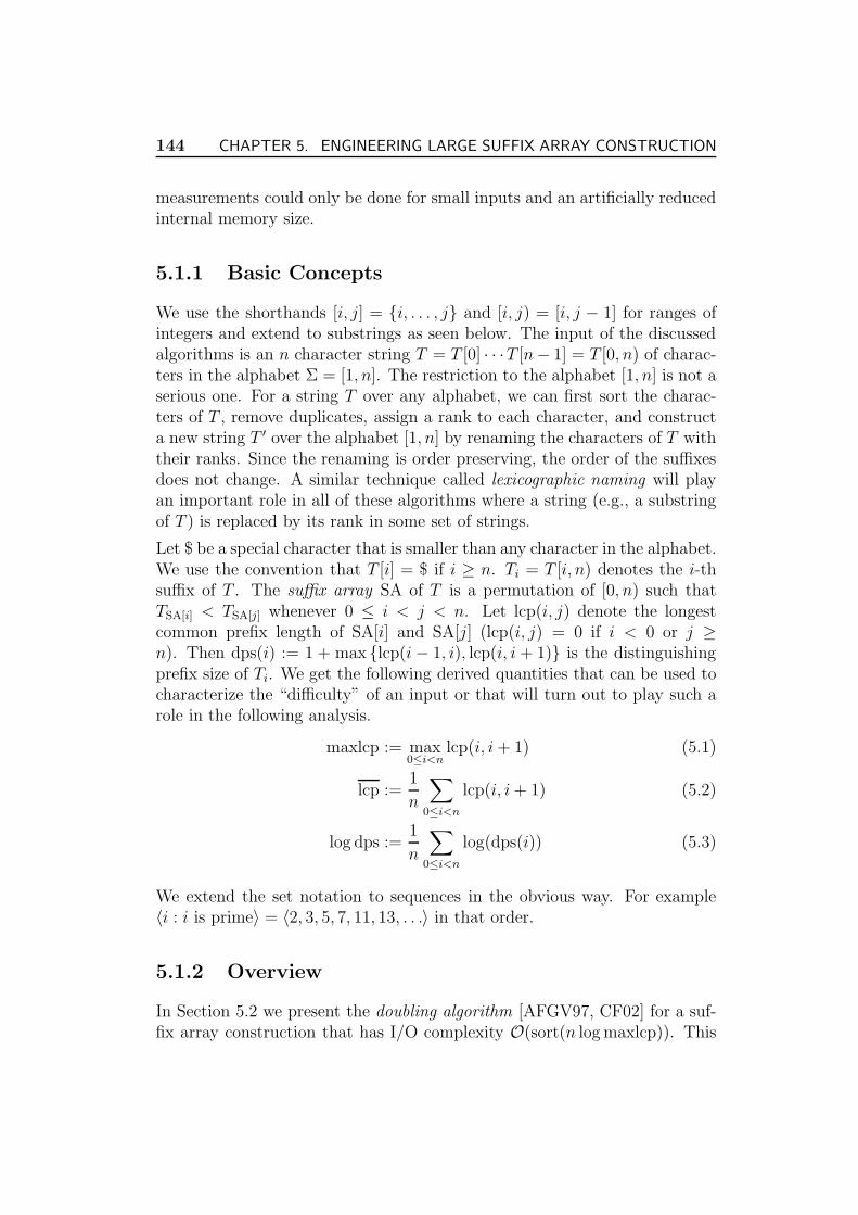
144 CHAPTER 5. ENGINEERING LARGE SUFFIX ARRAY CONSTRUCTION
measurements could only be done for small inputs and an artificially reducedinternal memory size.
5.1.1 Basic Concepts
We use the shorthands [i, j] = i, . . . , j and [i, j) = [i, j − 1] for ranges ofintegers and extend to substrings as seen below. The input of the discussedalgorithms is an n character string T = T [0] · · ·T [n− 1] = T [0, n) of charac-ters in the alphabet Σ = [1, n]. The restriction to the alphabet [1, n] is not aserious one. For a string T over any alphabet, we can first sort the charac-ters of T , remove duplicates, assign a rank to each character, and constructa new string T ′ over the alphabet [1, n] by renaming the characters of T withtheir ranks. Since the renaming is order preserving, the order of the suffixesdoes not change. A similar technique called lexicographic naming will playan important role in all of these algorithms where a string (e.g., a substringof T ) is replaced by its rank in some set of strings.
Let $ be a special character that is smaller than any character in the alphabet.We use the convention that T [i] = $ if i ≥ n. Ti = T [i, n) denotes the i-thsuffix of T . The suffix array SA of T is a permutation of [0, n) such thatTSA[i] < TSA[j] whenever 0 ≤ i < j < n. Let lcp(i, j) denote the longestcommon prefix length of SA[i] and SA[j] (lcp(i, j) = 0 if i < 0 or j ≥n). Then dps(i) := 1 + max lcp(i − 1, i), lcp(i, i + 1) is the distinguishingprefix size of Ti. We get the following derived quantities that can be used tocharacterize the “difficulty” of an input or that will turn out to play such arole in the following analysis.
maxlcp := max0≤i<n
lcp(i, i + 1) (5.1)
lcp :=1
n
∑
0≤i<n
lcp(i, i + 1) (5.2)
log dps :=1
n
∑
0≤i<n
log(dps(i)) (5.3)
We extend the set notation to sequences in the obvious way. For example〈i : i is prime〉 = 〈2, 3, 5, 7, 11, 13, . . .〉 in that order.
5.1.2 Overview
In Section 5.2 we present the doubling algorithm [AFGV97, CF02] for a suf-fix array construction that has I/O complexity O(sort(n log maxlcp)). This

5.2. DOUBLING ALGORITHM 145
algorithm sorts strings of size 2k in the k-th iteration. This variant alreadyyields some small optimization opportunities.
Section 5.3 gives a simple and efficient way to discard suffixes from fur-ther iterations of the doubling algorithm when their position in the suffixarray is already known. This leads to an algorithm with I/O complexityO(sort(n log dps)), improving on a previous discarding algorithm with I/Ocomplexity O(sort(n log dps) + scan(n log maxlcp)) [CF02]. A further con-stant factor is gained in Section 5.4 by considering a generalization of thedoubling technique that sorts strings of size ak in iteration k. The bestmultiplication factor is four (quadrupling) or five. A pipelined optimal algo-rithm with I/O complexity O(sort(n)) in Section 5.5 and its generalizationin Section 5.6 conclude our sequence of suffix array construction algorithms.
A useful tool for testing our implementations was a fast and simple externalmemory checker for suffix arrays described in Section 5.7.
In Section 5.8 we report on extensive experiments using synthetic difficultinputs, the human genome, English books, web-pages, and program sourcecode using inputs of up to 4 GByte on a low cost machine and a faster high-end system. The theoretically optimal algorithm turns out to be the winnerclosely followed by quadrupling with discarding.
Section 5.10 summarizes the overall results and discusses how even largersuffix arrays could be build.
5.2 Doubling Algorithm
Figure 5.1 shows a pseudocode for the doubling algorithm [AFGV97, CF02].The basic idea is to replace characters T [i] of the input by lexicographic namesthat respect the lexicographic order of the length 2k substring T [i, i + 2k) inthe k-th iteration. In contrast to previous variants of this algorithm, thisformulation never actually builds the resulting string of names. Rather, itmanipulates a sequence P of pairs (c, i) where each name c is tagged with itsposition i in the input. To obtain names for the next iteration k+1, the namesfor T [i, i+2k) and T [i+2k, i+2k+1) together with the position i are stored ina sequence S and sorted. The new names can now be obtained by scanningthis sequence and comparing adjacent tuples. Sequence S can be build usingconsecutive elements of P if we sort P using the pair (i mod 2k, i div 2k).Previous formulations of the algorithm use i as a sorting criterion and there-fore have to access elements that are 2k characters apart. Our approach savesI/Os and simplifies the pipelined implementation.
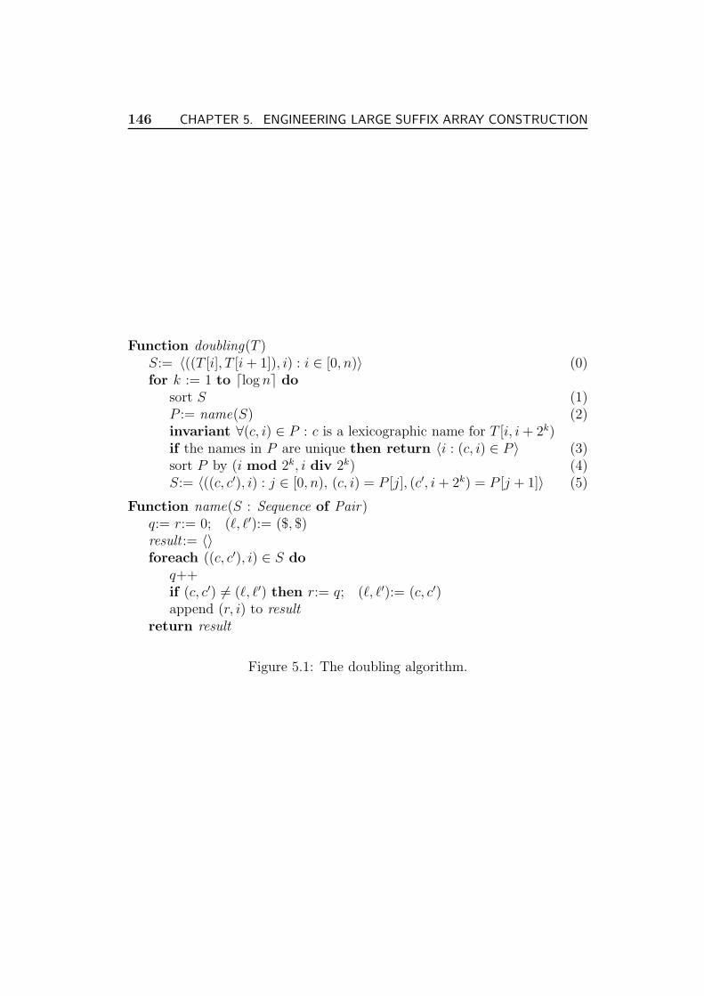
146 CHAPTER 5. ENGINEERING LARGE SUFFIX ARRAY CONSTRUCTION
Function doubling(T )S:= 〈((T [i], T [i + 1]), i) : i ∈ [0, n)〉 (0)for k := 1 to ⌈log n⌉ do
sort S (1)P := name(S) (2)invariant ∀(c, i) ∈ P : c is a lexicographic name for T [i, i + 2k)if the names in P are unique then return 〈i : (c, i) ∈ P 〉 (3)sort P by (i mod 2k, i div 2k) (4)S:= 〈((c, c′), i) : j ∈ [0, n), (c, i) = P [j], (c′, i + 2k) = P [j + 1]〉 (5)
Function name(S : Sequence of Pair)q:= r:= 0; (ℓ, ℓ′):= ($, $)result := 〈〉foreach ((c, c′), i) ∈ S do
q++if (c, c′) 6= (ℓ, ℓ′) then r:= q; (ℓ, ℓ′):= (c, c′)append (r, i) to result
return result
Figure 5.1: The doubling algorithm.

5.3. DISCARDING 147
The algorithm performs a constant number of sorting and scanning opera-tions for sequences of size n in each iteration. The number of iterations isdetermined by the logarithm of the longest common prefix.
Theorem 10 ([DKMS06]). The doubling algorithm from Figure 5.1 can beimplemented to run using sort(5n) ⌈log(1 + maxlcp)⌉ + O(sort(n)) I/Os.
Proof. The following pipelined data flow graph shows that each iteration canbe implemented using sort(2n)+sort(3n) ≤ sort(5n) I/Os. The numbers referto the line numbers in Figure 5.1.
1 2 543n 2n
sorting nodenodestreaming
After ⌈log(1 + maxlcp)⌉ iterations, the algorithm finishes. The O(sort(n))term accounts for the I/Os needed in Line 0 and for computing the finalresult. Note that there is a small technicality here: Although naming can findout “for free” whether all names are unique, the result is known only whennaming finishes. However, at this time, the first phase of the sorting stepin Line 4 has also finished and has already incurred some I/Os. Moreover,the convenient arrangement of the pairs in P is destroyed now. However, wecan then abort the sorting process, undo the wrong sorting, and compute thecorrect output.
5.3 Discarding
The paper [DKMS06] present a new discarding algorithm for computing suffixarrays. With the help of Stxxl pipelining the algorithm can be implementedwith very small constant factors in I/O volume.
Let cki be the lexicographic name of T [i, i+2k), i.e., the value paired with i at
iteration k in Figure 5.1. Since cki is the number of strictly smaller substrings
of length 2k, it is a non-decreasing function of k. More precisely, ck+1i − ck
i isthe number of positions j such that ck
j = cki but ck
j+2k < cki+2k . This provides
an alternative way of computing the names given in Figure 5.3.
Another consequence of the above observation is that if cki is unique, i.e.,
ckj 6= ck
i for all j 6= i, then chi = ck
i for all h > k. The idea of the discardingalgorithm is to take advantage of this, i.e., discard pair (c, i) from further
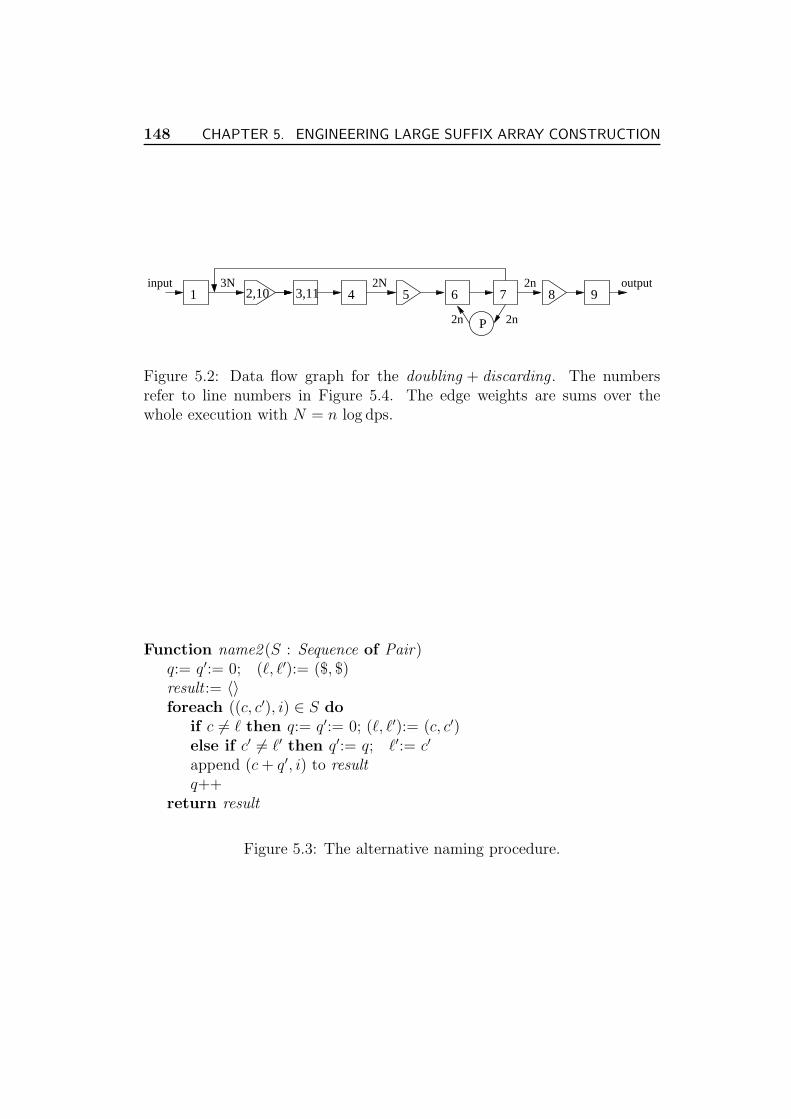
148 CHAPTER 5. ENGINEERING LARGE SUFFIX ARRAY CONSTRUCTION
2,10 3,11 4 5 6 71
P
983N 2N 2ninput
2n2n
output
Figure 5.2: Data flow graph for the doubling + discarding. The numbersrefer to line numbers in Figure 5.4. The edge weights are sums over thewhole execution with N = n log dps.
Function name2 (S : Sequence of Pair)q:= q′:= 0; (ℓ, ℓ′):= ($, $)result := 〈〉foreach ((c, c′), i) ∈ S do
if c 6= ℓ then q:= q′:= 0; (ℓ, ℓ′):= (c, c′)else if c′ 6= ℓ′ then q′:= q; ℓ′:= c′
append (c + q′, i) to resultq++
return result
Figure 5.3: The alternative naming procedure.
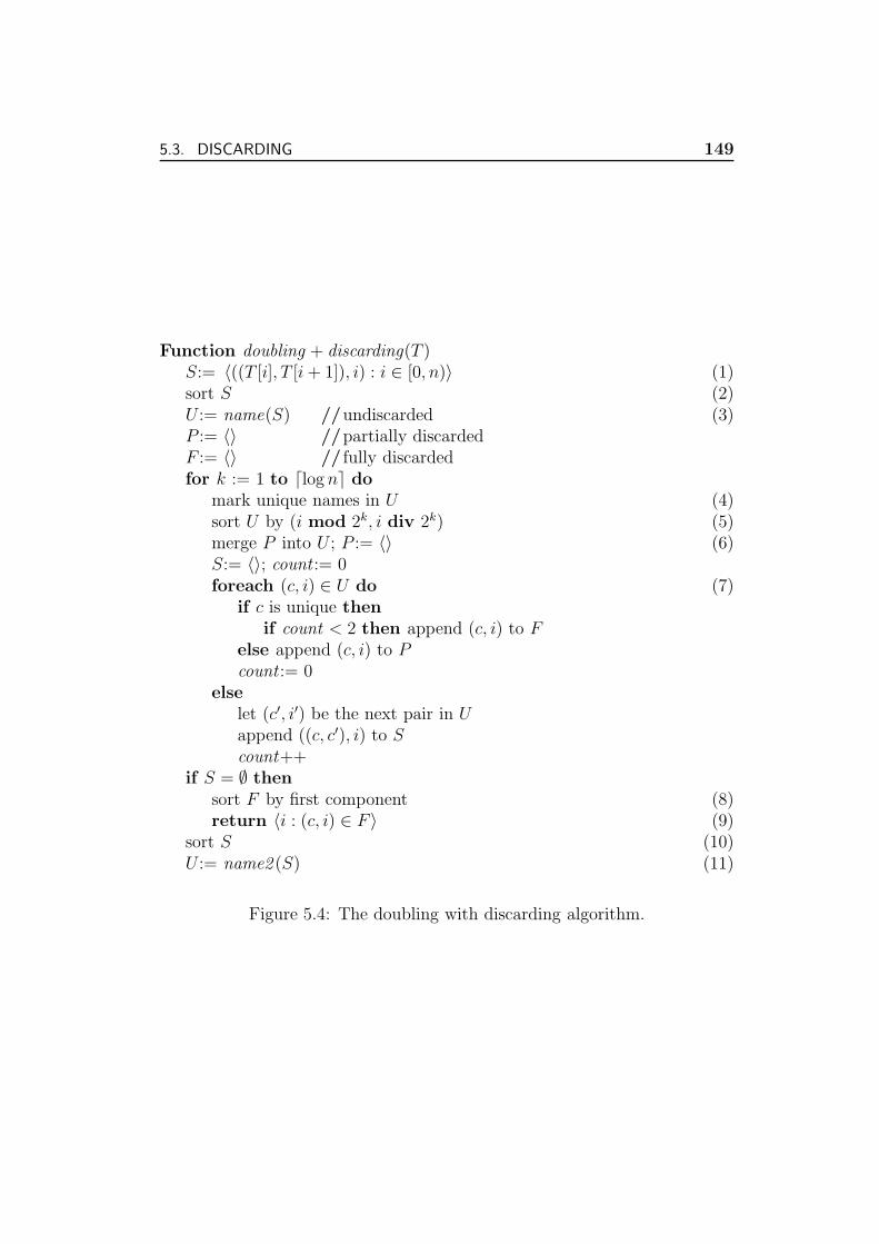
5.3. DISCARDING 149
Function doubling + discarding(T )S:= 〈((T [i], T [i + 1]), i) : i ∈ [0, n)〉 (1)sort S (2)U := name(S) //undiscarded (3)P := 〈〉 //partially discardedF := 〈〉 // fully discardedfor k := 1 to ⌈log n⌉ do
mark unique names in U (4)sort U by (i mod 2k, i div 2k) (5)merge P into U ; P := 〈〉 (6)S:= 〈〉; count := 0foreach (c, i) ∈ U do (7)
if c is unique thenif count < 2 then append (c, i) to F
else append (c, i) to Pcount := 0
elselet (c′, i′) be the next pair in Uappend ((c, c′), i) to Scount++
if S = ∅ thensort F by first component (8)return 〈i : (c, i) ∈ F 〉 (9)
sort S (10)U := name2 (S) (11)
Figure 5.4: The doubling with discarding algorithm.
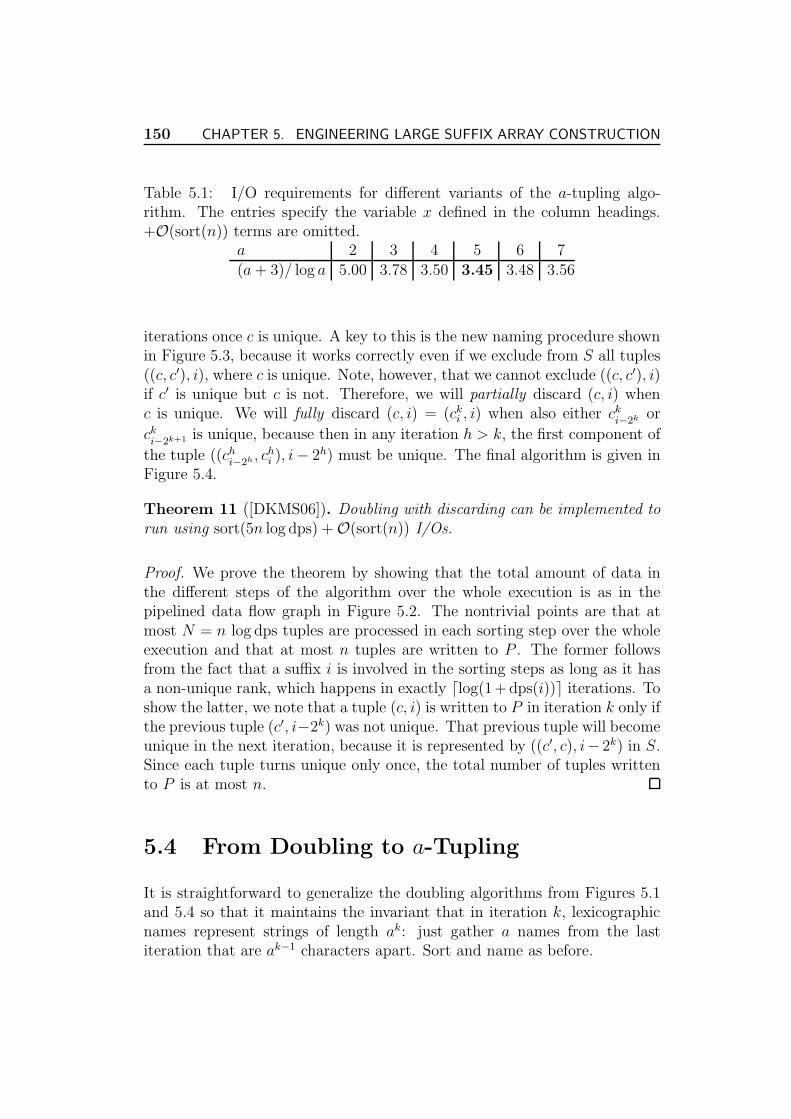
150 CHAPTER 5. ENGINEERING LARGE SUFFIX ARRAY CONSTRUCTION
Table 5.1: I/O requirements for different variants of the a-tupling algo-rithm. The entries specify the variable x defined in the column headings.+O(sort(n)) terms are omitted.
a 2 3 4 5 6 7(a + 3)/ log a 5.00 3.78 3.50 3.45 3.48 3.56
iterations once c is unique. A key to this is the new naming procedure shownin Figure 5.3, because it works correctly even if we exclude from S all tuples((c, c′), i), where c is unique. Note, however, that we cannot exclude ((c, c′), i)if c′ is unique but c is not. Therefore, we will partially discard (c, i) whenc is unique. We will fully discard (c, i) = (ck
i , i) when also either cki−2k or
cki−2k+1 is unique, because then in any iteration h > k, the first component of
the tuple ((chi−2h, c
hi ), i− 2h) must be unique. The final algorithm is given in
Figure 5.4.
Theorem 11 ([DKMS06]). Doubling with discarding can be implemented torun using sort(5n log dps) + O(sort(n)) I/Os.
Proof. We prove the theorem by showing that the total amount of data inthe different steps of the algorithm over the whole execution is as in thepipelined data flow graph in Figure 5.2. The nontrivial points are that atmost N = n log dps tuples are processed in each sorting step over the wholeexecution and that at most n tuples are written to P . The former followsfrom the fact that a suffix i is involved in the sorting steps as long as it hasa non-unique rank, which happens in exactly ⌈log(1+dps(i))⌉ iterations. Toshow the latter, we note that a tuple (c, i) is written to P in iteration k only ifthe previous tuple (c′, i−2k) was not unique. That previous tuple will becomeunique in the next iteration, because it is represented by ((c′, c), i− 2k) in S.Since each tuple turns unique only once, the total number of tuples writtento P is at most n.
5.4 From Doubling to a-Tupling
It is straightforward to generalize the doubling algorithms from Figures 5.1and 5.4 so that it maintains the invariant that in iteration k, lexicographicnames represent strings of length ak: just gather a names from the lastiteration that are ak−1 characters apart. Sort and name as before.

5.5. I/O-OPTIMAL PIPELINED DC3 ALGORITHM 151
The pseudocode of the generalized doubling algorithm without discarding ispresented in Figure 5.5.
Theorem 12 ([DKMS06]). The a-tupling algorithm can be implemented torun using
sort(a + 3
log an) log maxlcp + O(sort(n)) or
sort(a + 3
log an) log dps + O(sort(n))
I/Os without or with discarding respectively.
We get a tradeoff between higher cost for each iteration and a smaller numberof iterations that is determined by the ratio a+3
log a. Evaluating this expression
we get the optimum for a = 5 (Table 5.1). But the value for a = 4 is only1.5 % worse, needs less memory, and calculations are much easier becausefour is a power two. Hence, we choose a = 4 for our implementation of thea-tupling algorithm. This quadrupling algorithm needs 30 % less I/Os thandoubling.
Function atupling(T )S:= 〈((T [i], T [i + 1], . . . , T [i + a − 1)]), i) : i ∈ [0, n)〉for k := 1 to ⌈logan⌉ do
sort SP := name(S)invariant ∀(c, i) ∈ P :c is a lexicographic name for T [i, i + ak)if the names in P are unique then return 〈i : (c, i) ∈ P 〉sort P by (i mod ak, i div ak))S:= 〈((c0, . . . , cq, . . . , ca−1), i) : j ∈ [0, n),
(cq, i + q · ak) = P [j + q], q ∈ [0, a)〉
Figure 5.5: The a-tupling algorithm.
5.5 I/O-Optimal Pipelined DC3 Algorithm
The following three-step algorithm outlines a linear time algorithm for suffixarray construction [KSB06]:
152 CHAPTER 5. ENGINEERING LARGE SUFFIX ARRAY CONSTRUCTION
1. Construct the suffix array of the suffixes starting at positions i mod 3 6=0. This is done by reduction to the suffix array construction of a stringof two thirds the length, which is solved recursively.
2. Construct the suffix array of the remaining suffixes using the result ofthe first step.
3. Merge the two suffix arrays into one.
Figure 5.6 gives a pseudocode for an external implementation of this algo-rithm and Figure 5.7 gives a data flow graph that allows pipelined execution.Step 1 is implemented by Lines (1)–(6) and starts out quite similar to thetripling (3-tupling) algorithm described in Section 5.4. The main differenceis that triples are only obtained for two thirds of the suffixes and that weuse recursion to find lexicographic names that characterize the relative orderof these sample suffixes exactly. As a preparation for the Steps 2 and 3, inlines (7)–(10) these sample names are used to annotate each suffix positioni with enough information to determine its global rank. More precisely, atmost two sample names and the first one or two characters suffice to com-pletely determine the rank of a suffix. This information can be obtained I/Oefficiently by simultaneously scanning the input and the names of the samplesuffixes sorted by their position in the input. With this information, Step 2reduces to sorting suffixes Ti with i mod 3 = 0 by their first character andthe name for Ti+1 in the sample (Line 11). Line (12) reconstructs the orderof the mod-2 suffixes and mod-3 suffixes. Line (13) implements Step 3 by or-dinary comparison based merging. The slight complication is the comparisonfunction. There are three cases:
• A mod-0 suffix Ti can be compared with a mod-1 suffix Tj by lookingat the first characters and the names for Ti+1 and Tj+1 in the sample,respectively.
• For a comparison between a mod-0 suffix Ti and a mod-2 suffix Tj theabove technique does not work since Tj+1 is not in the sample. However,both Ti+2 and Tj+2 are in the sample so that it suffices to look at thefirst two characters and the names of Ti+2 and Tj+2 respectively.
• Mod-1 suffixes and Mod-2 suffixes can be compared by looking at theirnames in the sample.
The resulting pipelined data flow graph is large but fairly straightforwardexcept for the file node which stores a copy of input stream T . The problem isthat the input is needed twice. First, Line 2 uses it for generating the sample

5.5. I/O-OPTIMAL PIPELINED DC3 ALGORITHM 153
and later, the node implementing Lines (8)–(10) scans it simultaneously withthe names of the sample suffixes. It is not possible to pipeline both scans,however, this problem can be solved by writing a temporary copy of the inputstream. Note that this is still cheaper than using a file representation for theinput since this would mean that this file is read twice. We are now readyto analyze the I/O complexity of the algorithm.
Function DC3 (T )S:= 〈((T [i, i + 2]), i) : i ∈ [0, n), i mod 3 6= 0〉 //mod12 suffixes (1)sort S by the first component // sort triples (2)P := name(S) //name triples (3)if the names in P are not unique then
sort the (i, r) ∈ P by (i mod 3, i div 3) //build rec. input (4)SA12:= DC3 (〈c : (c, i) ∈ P 〉) // recurse (5)P :=
⟨
(j + 1, SA12[j]) : j ∈ [0, 2n/3)⟩
(6)sort P by the second component // inv. SA of sample (7)S0:= 〈(T [i], T [i + 1], c′, c′′, i) : i mod 3 = 0, (c′, i + 1), (c′′, i + 2) ∈ P 〉 (8)S1:= 〈(c, T [i], c′, i) : i mod 3 = 1, (c, i), (c′, i + 1) ∈ P 〉 (9)S2:= 〈(c, T [i], T [i + 1], c′′, i) : i mod 3 = 2, (c, i), (c′′, i + 2) ∈ P 〉 (10)sort S0 by components 1,3 // sort mod0 suff. (11)sort S1 and S2 by component 1 // resort mod12 suff. (12)S:= merge(S0, S1, S2) using comparison function: (13)
(t, t′, c′, c′′, i) ∈ S0 ≤ (d, u, d′, j) ∈ S1 ⇔ (t, c′) ≤ (u, d′)(t, t′, c′, c′′, i) ∈ S0 ≤ (d, u, u′, d′′, j) ∈ S2 ⇔ (t, t′, c′′) ≤ (u, u′, d′′)(c, t, c′, i) ∈ S1 ≤ (d, u, u′, d′′, j) ∈ S2 ⇔ c ≤ d
return 〈last component of s : s ∈ S〉 (14)
Figure 5.6: The DC3-algorithm.
Theorem 13 ([DKMS06]). The DC3 algorithm from Figure 5.6 can be im-plemented to run using sort(30n) + scan(6n) I/Os.
Proof. Let V (n) denote the number of I/Os for the external DC3 algorithm.Using the pipelined data flow diagram from Figure 5.7 we can conclude that
V (n) ≤ sort((83
+ 43
+ 43
+ 53
+ 43
+ 53)n) + scan(2n) + V (2
3n)
= sort(10n) + scan(2n) + V (23n)
This recurrence has the solution V (n) ≤ 3(sort(10n) + scan(2n)) ≤sort(30n) + scan(6n). Note that the data flow diagram assumes that the

154 CHAPTER 5. ENGINEERING LARGE SUFFIX ARRAY CONSTRUCTION
filenode
streaming node
T
recursionsortingnode
8n3
4n3
12
11
12
13 144n3
5n3
5n3
4n3
321
inputif names are not unique
8−105 6 7
output
nn
4
Figure 5.7: Data flow graphs for the DC3 algorithm. The numbers refer toline numbers in Figure 5.6.
input is a data stream into the procedure call. However, we get the samecomplexity if the original input is a file. In that case, we have to read theinput once but we save writing it to the local file node T .
5.6 Generalized Difference Cover Algorithm
DC3 computes the suffix array of the two-thirds of the suffixes in its recursion.In the generalized algorithm DCX [KSB06] one tries to reduce the numberof sample suffixes, which might decrease the cost of the recursion.
The algorithm DCX chooses the sample of suffixes starting at indexes IX =i | i mod X ∈ CX (for DC3 X = 3 and C3 = 1, 2). For any given Xthe set CX must be chosen such that |CX | is minimal and the order of theremaining suffixes can be reconstructed using the sample suffixes. To fulfillthese requirements one uses the minimum difference covers [Haa04] of ZX
(ZX is the set of integers modulo X). For a subset C ′ of a finite Abeliangroup G, we define d(C ′) = a − b | a, b ∈ C ′. If d(C ′) = G, we call C ′ adifference cover of G. [Haa04] contains minimum difference covers C ′
X ofZX for primes X up to 133 (see also Table 5.2). The algorithm DCX setsCX = j |X − j − 1 ∈ C ′
X.Now we find the number of I/Os needed by a recursion of the DCX algorithm:
sorting S by T [i, i+X −1] (Line (2) in Figure 5.6) costs sort((X +1)n · |CX |X
)I/Os, writing and reading T takes scan(2n) I/Os, building the input for
the recursion (Line (4)) needs sort(2n · |CX |X
) I/Os, permuting in Line (7)
incurs sort(2n · |CX |X
) I/Os, sorting the merge tuples (Lines (11)–(12)) needssort(δXn) I/Os, where δX is the average merge tuple size (e. g. δ3 = 5+4+5
3).
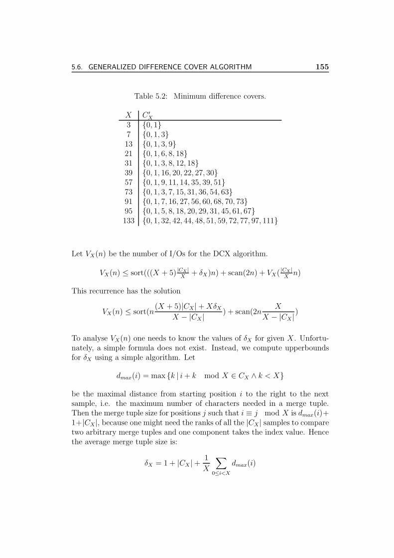
5.6. GENERALIZED DIFFERENCE COVER ALGORITHM 155
Table 5.2: Minimum difference covers.
X C ′X
3 0, 17 0, 1, 313 0, 1, 3, 921 0, 1, 6, 8, 1831 0, 1, 3, 8, 12, 1839 0, 1, 16, 20, 22, 27, 3057 0, 1, 9, 11, 14, 35, 39, 5173 0, 1, 3, 7, 15, 31, 36, 54, 6391 0, 1, 7, 16, 27, 56, 60, 68, 70, 7395 0, 1, 5, 8, 18, 20, 29, 31, 45, 61, 67133 0, 1, 32, 42, 44, 48, 51, 59, 72, 77, 97, 111
Let VX(n) be the number of I/Os for the DCX algorithm.
VX(n) ≤ sort(((X + 5) |CX |X
+ δX)n) + scan(2n) + VX( |CX |X
n)
This recurrence has the solution
VX(n) ≤ sort(n(X + 5)|CX| + XδX
X − |CX |) + scan(2n
X
X − |CX |)
To analyse VX(n) one needs to know the values of δX for given X. Unfortu-nately, a simple formula does not exist. Instead, we compute upperboundsfor δX using a simple algorithm. Let
dmax(i) = max k | i + k mod X ∈ CX ∧ k < X
be the maximal distance from starting position i to the right to the nextsample, i.e. the maximum number of characters needed in a merge tuple.Then the merge tuple size for positions j such that i ≡ j mod X is dmax(i)+1+|CX|, because one might need the ranks of all the |CX | samples to comparetwo arbitrary merge tuples and one component takes the index value. Hencethe average merge tuple size is:
δX = 1 + |CX | +1
X
∑
0≤i<X
dmax(i)
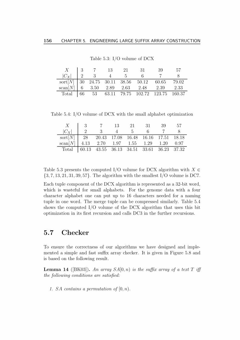
156 CHAPTER 5. ENGINEERING LARGE SUFFIX ARRAY CONSTRUCTION
Table 5.3: I/O volume of DCX
X 3 7 13 21 31 39 57|CX | 2 3 4 5 6 7 8
sort[N ] 30 24.75 30.11 38.56 50.12 60.65 79.02scan[N ] 6 3.50 2.89 2.63 2.48 2.39 2.33Total 66 53 63.11 79.75 102.72 123.75 160.37
Table 5.4: I/O volume of DCX with the small alphabet optimization
X 3 7 13 21 31 39 57|CX | 2 3 4 5 6 7 8
sort[N ] 28 20.43 17.08 16.48 16.16 17.51 18.18scan[N ] 4.13 2.70 1.97 1.55 1.29 1.20 0.97Total 60.13 43.55 36.13 34.51 33.61 36.23 37.32
Table 5.3 presents the computed I/O volume for DCX algorithm with X ∈3, 7, 13, 21, 31, 39, 57. The algorithm with the smallest I/O volume is DC7.
Each tuple component of the DCX algorithm is represented as a 32-bit word,which is wasteful for small alphabets. For the genome data with a fourcharacter alphabet one can put up to 16 characters needed for a namingtuple in one word. The merge tuple can be compressed similarly. Table 5.4shows the computed I/O volume of the DCX algorithm that uses this bitoptimization in its first recursion and calls DC3 in the further recursions.
5.7 Checker
To ensure the correctness of our algorithms we have designed and imple-mented a simple and fast suffix array checker. It is given in Figure 5.8 andis based on the following result.
Lemma 14 ([BK03]). An array SA[0, n) is the suffix array of a text T iffthe following conditions are satisfied:
1. SA contains a permutation of [0, n).
5.8. EXPERIMENTS 157
2. ∀i, j : ri ≤ rj ⇔ (T [i], ri+1) ≤ (T [j], rj+1) where ri denotes the rank ofthe suffix Si according to the suffix array.
Function Checker(SA, T )P := 〈(SA[i], i + 1) : i ∈ [0, n)〉 (1)sort P by the first component (2)if 〈i : (i, r) ∈ P 〉 6= [0, n) then return falseS:= [(r, (T [i], r′)) : i ∈ [0, n), (3)
(i, r) = P [i], (i + 1, r′) = P [i + 1]]sort S by the first component (4)if 〈(c, r′) : (r, (c, r′)) ∈ S〉 is sorted (5)then return true else return false
Figure 5.8: The suffix array checker.
Theorem 15. The suffix array checker from Figure 5.8 can be implementedto run using sort(5n) + scan(2n) I/Os.
5.8 Experiments
We have implemented the algorithms (except DCX) in C++ using the g++3.2.3 compiler (optimization level -O2 -fomit-frame-pointer)1 and the ex-ternal memory library Stxxl Version 0.52 [Dem, DKS05a]. We have run theexperiments on two platforms. The first system has two 2.0 GHz Intel Xeonprocessors (our implementations only use one processor), one GByte of RAMand eight 80 GByte ATA IBM 120GXP disks. Refer to [DS03] for a perfor-mance evaluation of this machine whose cost was 2500 Euro in July 2002. Thesecond platform is a high-end SMP system with four 64-bit AMD Opteron1.8 GHz processors, 8 GByte of RAM (we use only one GByte) and eight 73GByte SCSI Seagate 15000 RPM ST373453LC disks. In our experiments weused four disks if not specified otherwise.
Table 5.5 shows the considered input instances.We have collected some of these instances athttp://algo2.iti.uka.de/dementiev/esuffix/instances.shtml andftp://www.mpi-sb.mpg.de/pub/outgoing/sanders/. For a nonsynthetic
1 The sources are available underhttp://algo2.iti.uka.de/dementiev/esuffix/docu/index.html.
158 CHAPTER 5. ENGINEERING LARGE SUFFIX ARRAY CONSTRUCTION
Name DescriptionRandom2 Two concatenated copies of a Random string of length
n/2. This is a difficult instance that is hard to beatusing simple heuristics.
Gutenberg Freely available English texts fromhttp://promo.net/pg/list.html.
Genome The known pieces of the human genome fromhttp://genome.ucsc.edu/downloads.html (sta-tus May, 2004). We have normalized this input toignore the distinction between upper case and lowercase letters. The result are characters in an alphabetof size 5 (ACGT and sometimes long sequences of“unknown” characters).
HTML Pages from a web crawl containing only pages from .gov
domains. These pages are filtered so that only text andhtml code is contained but no pictures and no binaryfiles.
Source Source code (mostly C++) containing coreutils, gcc,gimp, kde, xfree, emacs, gdb, Linux kernel and OpenOffice).
Table 5.5: Input instances.
Table 5.6: Statistics of the instances used in the experiments.
T n = |T | |Σ| maxlcp lcp log dpsRandom2 232 128 231 ≈ 229 ≈ 29.56Gutenberg 3 277 099 765 128 4 819 356 45 617 10.34
Genome 3 070 128 194 5 21 999 999 454 111 6.53
HTML 4 214 295 245 128 102 356 1 108 6.99
Source 547 505 710 128 173 317 431 5.80
instance T of length n, our experiments use T itself and its prefixes of theform T [0, 2i). Table 5.6 and Figure 5.9 show statistics of the properties ofthese instances.
Figure 5.10 shows the execution time and the I/O volume side by side, foreach of our instance families and for the algorithms nonpipelined doubling,pipelined doubling, pipelined doubling with discarding, pipelined quadru-

5.8. EXPERIMENTS 159
0
2
4
6
8
10
232230228226224
loga
rithm
ic lc
p
n
GutenbergHtml
Open SourceGenome
Figure 5.9: Statistics of the instances used in the experiments.
pling, pipelined quadrupling with discarding2, and DC3 running on the Xeonmachine. All ten plots share the same x-axis and the same curve labels. Com-puting all these instances takes about 14 days moving more than 20 TByteof data. Due to these large execution times it was not feasible to run allalgorithms for all input sizes and all instances. However, there is enoughdata to draw some interesting conclusions.
Complicated behavior is observed for “small” inputs up to 226 characters.The main reason is that we made no particular effort to optimize special caseswhere at least some part of some algorithm could execute internally. Some-times Stxxl makes such optimizations, e.g. automatically sorting smallinputs in the internal memory. Another factor is the constant start-up over-head of stxxl::vectors which amortizes only with larger inputs. The gran-ularity with which stxxl::vector loads and stores blocks from/to externalmemory was not optimized for small inputs.
The most important observation is that the DC3-algorithm is always thefastest algorithm and is almost completely insensitive to the input. For allinputs of a size of more than a GByte, DC3 is at least twice as fast asits closest competitor. With respect to the I/O volume, DC3 is sometimesequaled by quadrupling with discarding. This happens for relatively small
2The discarding algorithms we have implemented need slightly more I/Os and perhapsmore complex calculations than the newer algorithms described in Section 5.3.
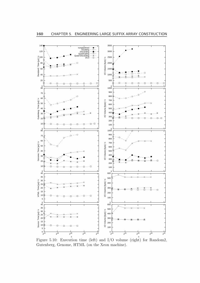
160 CHAPTER 5. ENGINEERING LARGE SUFFIX ARRAY CONSTRUCTION
0
20
40
60
80
100
120
140
Ran
dom
2: T
ime
[µs]
/ n
nonpipelinedDoubling
DiscardingQuadrupling
Quad-DiscardingDC3
0
500
1000
1500
2000
2500
3000
3500
I/O V
olum
e [b
yte]
/ n
0
10
20
30
40
50
60
70
80
Gut
enbe
rg: T
ime
[µs]
/ n
0
100
200
300
400
500
600
700
800
900
1000
I/O V
olum
e [b
yte]
/ n
0
10
20
30
40
50
60
70
80
Gen
ome:
Tim
e [µ
s] /
n
0
100
200
300
400
500
600
700
800
900
1000
I/O V
olum
e [b
yte]
/ n
0
5
10
15
20
25
30
35
40
HT
ML:
Tim
e [µ
s] /
n
0
100
200
300
400
500
600
I/O V
olum
e [b
yte]
/ n
0
5
10
15
20
25
30
35
40
224 226 228 230 232
Sou
rce:
Tim
e [µ
s] /
n
n
0
100
200
300
400
500
600
224 226 228 230 232
I/O V
olum
e [b
yte]
/ n
n
Figure 5.10: Execution time (left) and I/O volume (right) for Random2,Gutenberg, Genome, HTML (on the Xeon machine).
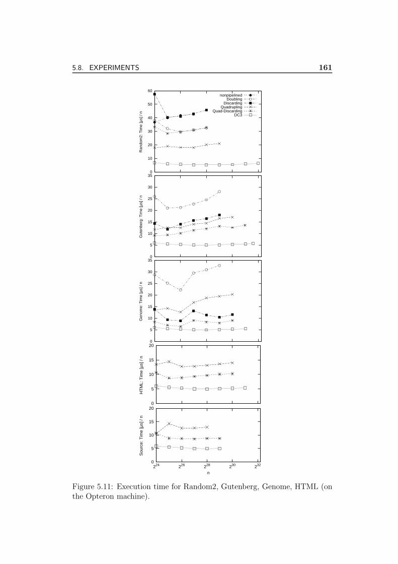
5.8. EXPERIMENTS 161
0
10
20
30
40
50
60
Ran
dom
2: T
ime
[µs]
/ n
nonpipelinedDoubling
DiscardingQuadrupling
Quad-DiscardingDC3
0
5
10
15
20
25
30
35
Gut
enbe
rg: T
ime
[µs]
/ n
0
5
10
15
20
25
30
35
Gen
ome:
Tim
e [µ
s] /
n
0
5
10
15
20
HT
ML:
Tim
e [µ
s] /
n
0
5
10
15
20
232230228226224
Sou
rce:
Tim
e [µ
s] /
n
n
Figure 5.11: Execution time for Random2, Gutenberg, Genome, HTML (onthe Opteron machine).
162 CHAPTER 5. ENGINEERING LARGE SUFFIX ARRAY CONSTRUCTION
inputs. Apparently quadrupling has more complex internal work.3 For ex-ample, it compares quadruples during half of its sorting operations whereasDC3 compares triples or pairs during sorting. For the difficult synthetic in-put Random2, quadrupling with discarding is by far outperformed by DC3.Even plain quadrupling, is much faster than quadrupling with discarding.This indicates that the internal logics for discarding is a bottleneck.
For real world inputs, discarding algorithms turn out to be successful com-pared to their nondiscarding counterparts. They outperform them both withrespect to the I/O volume and the running time. This could be explained bythe smaller log dps values according to Table 5.6. For random inputs withoutrepetitions the discarding algorithms might actually beat DC3 since one getsinputs with very small values of log dps.
Quadrupling algorithms consistently outperform doubling algorithms as pre-dicted by the analysis of the I/O complexity in Section 5.4.
Comparing pipelined doubling with nonpipelined doubling in the top pair ofplots (instance Random2) one can see that pipelining brings a huge reductionof the I/O volume, whereas the execution time is affected much less — aclear indication that our algorithms are dominated by internal calculations.However, in a setting with a slower I/O subsystem, e.g. a system with asingle disk, pipelining gives a significant speedup. Our experiments withD = 1 show that pipelined doubling is faster than its nonpipelined versionby a factor 1.9–2.4. We also have reasons to believe that our nonpipelinedsorter is more highly tuned than the pipelined one so that the advantageof pipelining may grow in future versions of Stxxl. We do not show thenonpipelined algorithm for the other inputs since the relative performancecompared to pipelined doubling should remain about the same.
A comparison of the new algorithms with previous algorithms is more dif-ficult. The implementation of [CF02] only works up to 2 GByte of totalexternal memory consumption and would thus have to compete with spaceefficient internal algorithms on our machine. At least we can compare theI/O volume per byte of input for the measurements in [CF02]. Their mostscalable algorithm for the largest real world input tested (26 MByte of textfrom the Reuters news agency) is nonpipelined doubling with partial dis-carding. This algorithm needs an I/O volume of 1303 Bytes per characterof input. The DC3-algorithm needs about 5 times less I/Os. Furthermore,it is to be expected that the lead gets bigger for larger inputs. The GBSalgorithm [GBYS92] needs 486 bytes of I/O per character for this input in
3One might also conclude that a similar increase in internal work could be expected inan implementation of the DC7 algorithm.

5.8. EXPERIMENTS 163
[CF02], i.e., even for this small input DC3 already outperforms the GBS al-gorithm. We can also attempt a speed comparison in terms of clock cyclesper byte of input. Here [CF02] needs 157, 000 cycles per byte for doublingwith simple discarding and 147, 000 cycles per byte for the GBS algorithmwhereas DC3 only needs about 20, 000 cycles. Again, the advantage shouldgrow for larger inputs in particular when comparing with the GBS algorithm.
The following small table shows the execution time of DC3 for 1 to 8 diskson the ‘Source’ instance on the Xeon machine.
D 1 2 4 6 8t[µs/byte] 13.96 9.88 8.81 8.65 8.52
We see that adding more disks only gives a very small speedup. (And wewould see very similar speedups for the other algorithms except nonpipelineddoubling). Even with 8 disks, DC3 has an I/O rate of less than 30 MByte/swhich is less than the peak performance of a single disk (45 MByte/s). Hence,by more effective overlapping of I/O and computation it should be possibleto sustain the performance of eight disks using a single cheap disk so thateven very cheap PCs could be used for external suffix array construction.
Figure 5.11 shows the execution times of the implementations running on theOpteron machine. The implementations need a factor of 1.7–2.4 less time.The largest speedup is observed for the quadrupling with discarding runningon the largest source code instance. This might be due to the faster SCSIhard disks with higher bandwidth (70 MB/s versus 45 MB/s) and the shorterseek time (3.6 ms versus 8.8 ms on average), and perhaps a faster 64-bit CPU.However, the relative performance of the algorithms remains the same as inthe experiments using the Xeon system.
5.8.1 The Checker
Figure 5.12 shows the execution time and the I/O volume of the suffix arraychecker from Section 5.7 running on the Opteron system. The horizontal axisdenotes the size of the input string T . The curves for the other input familiesare not shown, since the algorithm is not sensitive to the type of input. Theimplementation only needs 1–1.2 µs per input string character.
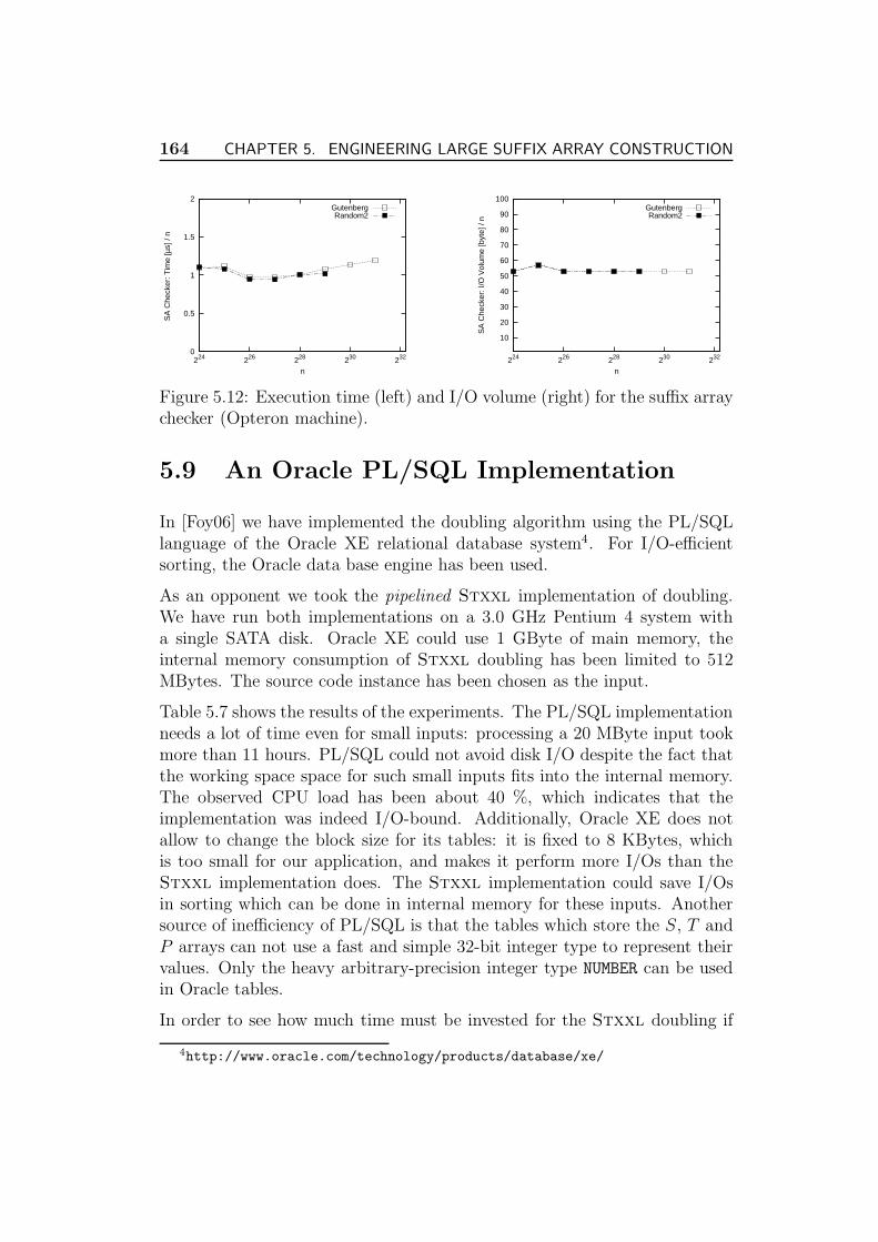
164 CHAPTER 5. ENGINEERING LARGE SUFFIX ARRAY CONSTRUCTION
0
0.5
1
1.5
2
232230228226224
SA
Che
cker
: Tim
e [µ
s] /
n
n
GutenbergRandom2
10
20
30
40
50
60
70
80
90
100
232230228226224
SA
Che
cker
: I/O
Vol
ume
[byt
e] /
n
n
GutenbergRandom2
Figure 5.12: Execution time (left) and I/O volume (right) for the suffix arraychecker (Opteron machine).
5.9 An Oracle PL/SQL Implementation
In [Foy06] we have implemented the doubling algorithm using the PL/SQLlanguage of the Oracle XE relational database system4. For I/O-efficientsorting, the Oracle data base engine has been used.
As an opponent we took the pipelined Stxxl implementation of doubling.We have run both implementations on a 3.0 GHz Pentium 4 system witha single SATA disk. Oracle XE could use 1 GByte of main memory, theinternal memory consumption of Stxxl doubling has been limited to 512MBytes. The source code instance has been chosen as the input.
Table 5.7 shows the results of the experiments. The PL/SQL implementationneeds a lot of time even for small inputs: processing a 20 MByte input tookmore than 11 hours. PL/SQL could not avoid disk I/O despite the fact thatthe working space space for such small inputs fits into the internal memory.The observed CPU load has been about 40 %, which indicates that theimplementation was indeed I/O-bound. Additionally, Oracle XE does notallow to change the block size for its tables: it is fixed to 8 KBytes, whichis too small for our application, and makes it perform more I/Os than theStxxl implementation does. The Stxxl implementation could save I/Osin sorting which can be done in internal memory for these inputs. Anothersource of inefficiency of PL/SQL is that the tables which store the S, T andP arrays can not use a fast and simple 32-bit integer type to represent theirvalues. Only the heavy arbitrary-precision integer type NUMBER can be usedin Oracle tables.
In order to see how much time must be invested for the Stxxl doubling if
4http://www.oracle.com/technology/products/database/xe/
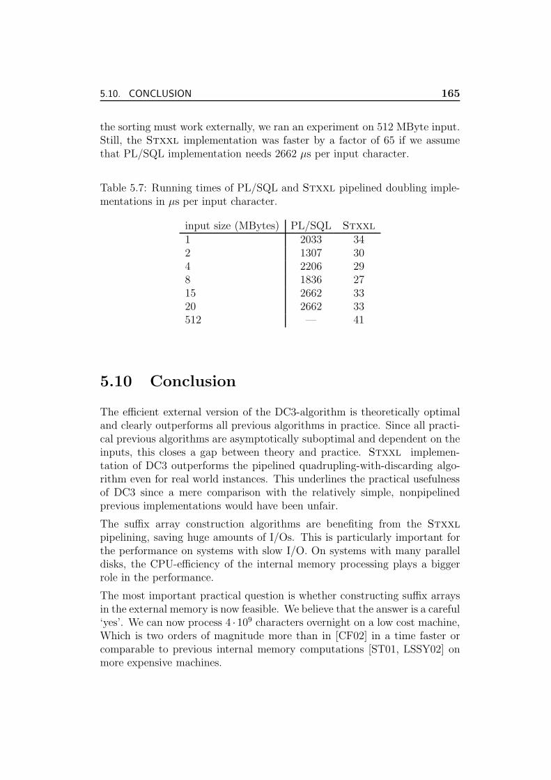
5.10. CONCLUSION 165
the sorting must work externally, we ran an experiment on 512 MByte input.Still, the Stxxl implementation was faster by a factor of 65 if we assumethat PL/SQL implementation needs 2662 µs per input character.
Table 5.7: Running times of PL/SQL and Stxxl pipelined doubling imple-mentations in µs per input character.
input size (MBytes) PL/SQL Stxxl
1 2033 342 1307 304 2206 298 1836 2715 2662 3320 2662 33512 — 41
5.10 Conclusion
The efficient external version of the DC3-algorithm is theoretically optimaland clearly outperforms all previous algorithms in practice. Since all practi-cal previous algorithms are asymptotically suboptimal and dependent on theinputs, this closes a gap between theory and practice. Stxxl implemen-tation of DC3 outperforms the pipelined quadrupling-with-discarding algo-rithm even for real world instances. This underlines the practical usefulnessof DC3 since a mere comparison with the relatively simple, nonpipelinedprevious implementations would have been unfair.
The suffix array construction algorithms are benefiting from the Stxxl
pipelining, saving huge amounts of I/Os. This is particularly important forthe performance on systems with slow I/O. On systems with many paralleldisks, the CPU-efficiency of the internal memory processing plays a biggerrole in the performance.
The most important practical question is whether constructing suffix arraysin the external memory is now feasible. We believe that the answer is a careful‘yes’. We can now process 4 ·109 characters overnight on a low cost machine,Which is two orders of magnitude more than in [CF02] in a time faster orcomparable to previous internal memory computations [ST01, LSSY02] onmore expensive machines.
166 CHAPTER 5. ENGINEERING LARGE SUFFIX ARRAY CONSTRUCTION
There are also many opportunities to scale to even larger inputs. In Sec-tion 5.6 we have outlined that for small alphabets, the generalized differencecover algorithm DCX, can yield significant further savings in I/O require-ments. With respect to the internal work, one could exploit that about halfof the sorting operations are just permutations. A better overlap betweenI/O and computation in future versions of pipelined Stxxl sorters shouldspeedup the implementations. More interestingly, there are many ways toparallelize. On a small scale, the pipelining paradigm allows us to run severalsorters and one streaming thread in parallel. On a large scale, DC3 is alsoperfectly parallelizable [KSB06]. An MPI-based [GLT98] distributed mem-ory implementation of DC3 [KS06] scales well up to 128 processors accordingto the experiments. It looks likely that the algorithm would also scale tothousands of processors. However, the parallel implementation does not useI/O-efficient processing, therefore this leaves room for further improvementswhich will enable a fast construction of even larger suffix arrays.
Chapter 6
Porting Algorithms to ExternalMemory
It turns out that some algorithms designed for the internal memory or forparallel computers can be directly adapted to run efficiently in the externalmemory. Such adaptation only includes a replacement of few underlyingnon-I/O-efficient algorithms by corresponding I/O-efficient versions.
We have already seen a 2-coloring algorithm in Section 4.7.7 where the re-placed algorithms were the spanning forest algorithm and the traversal ofthe trees using I/O-efficient Euler tour and list ranking algorithms. In thischapter, we show how to externalize a 5-coloring planar graph algorithmin Section 6.1 and an approximation algorithm for the maximum weightedmatching problem in Section 6.2. An extended example of an externalizationfor an algorithm finding perfect matchings in bipartite multigraphs is shownin Section 6.3.
6.1 5-Coloring Planar Graphs
A PRAM algorithm [HCD89] for 5-coloring planar graphs can be adopted torun in O(sort(n)) I/Os. It recursively colors the graph constructing a sub-problem which has at most a constant fraction of nodes of the input graph.The algorithm identifies a set of reducible nodes which are candidates forthe removal from the graph and also merges some of the nodes incident toreducible nodes, similarly to the algorithm in Section 4.7.6. The identifica-tion and the merging can be implemented in a constant number of sorting
167
168 CHAPTER 6. PORTING ALGORITHMS TO EXTERNAL MEMORY
and scanning steps. Not all of the candidates can be removed in a recur-sion, because there might be conflicts, e.g. if many reducible nodes decideto merge the same node. However, these conflicts might be resolved filteringsome candidate nodes out with a kind of maximal independent set com-putation in O(sort(n)) I/Os [Zeh02]. The remaining node set is still largeenough [HCD89] such that one has a constant-fraction graph reduction ineach recursion.
6.2 1/2-Approximation of Maximum
Weighted Matching
6.2.1 Definitions
A matching in graph G is a set of pairwise non-adjacent edges.
A maximal matching is a matching M of a graph G with the property thatif any edge not in M is added to M it is no longer a valid matching.
A maximum weighted matching is a matching where the sum of the weightsof the edges in the matching have a maximal value. There may be manymaximum weighted matchings.
A p-approximation algorithm of a maximization problem is an algorithmthat computes for any input instance I a solution with weight W , such that
WOPT(W )
≥ p, where OPT(W ) is the weight of an optimal solution for I.
6.2.2 The Algorithm
The internal memory greedy algorithm [Avi83] grows a maximal matching,choosing in each step the heaviest edge currently available, i.e. an edgenot incident to any of the already covered nodes. The algorithm runs inΘ(m log m) time since it requires sorting the edges of the graph by decreasingweight. This greedy algorithm produces an 1
2-approximation as shown in
[Avi83].
The algorithm can be externalized as follows:
1. sort the edges by decreasing weight using the I/O-efficient sorting,
2. assign unique ids to the edges numbering them according to the ob-tained order,
6.3. PERFECT MATCHINGS IN BIPARTITE MULTIGRAPHS 169
3. run the maximal matching algorithm from [Zeh02], but instead of theedge numbering proposed there, use the edge ids computed in the pre-vious step.
The maximal matching algorithm runs in O(sort(m + n)) I/Os [Zeh02],therefore the 1/2-approximation algorithm for finding a maximum weightedmatching only needs O(sort(m + n)) I/Os.
6.3 Perfect Matchings in Bipartite Multi-
graphs
6.3.1 Definitions
A multigraph is a graph which is permitted to have multiple edges, (alsocalled “parallel edges”) i.e. edges that have the same end nodes.
A perfect matching is a matching which covers all nodes of the (multi)graph.That is, every node of the (multi)graph is incident to exactly one edge of thematching.
A bipartite (multi)graph is a special (multi)graph where the set of nodescan be divided into two disjoint sets U and W such that every edge has oneend-point in U and one end-point in W .
An Euler partition is a partition of the edges into open and closed paths, sothat each node of an odd degree is at the end of exactly one open path, andeach node of an even degree is at the end of no open path.
An Euler split of a bipartite multigraph G = (V1, V2, E) is a pair of bipartitegraphs G1 = (V1, V2, E1) and G2 = (V1, V2, E2) where E1 and E2 are formedfrom an Euler partition by placing alternate edges of paths into E1 and E2.
A ∆-regular (multi)graph is a (multi)graph where each node has exactly ∆neighbors.
6.3.2 Introduction
Many efficient sequential algorithms for the problem have been developed.Cole [Col82] and Rizzi [Riz02] develop algorithms with a running timeO(m + n log n log ∆). There is also an EREW PRAM algorithm by Lev,Pippenger, and Valiant [LPV81] which requires O
(
log ∆ log2 n)
time and
170 CHAPTER 6. PORTING ALGORITHMS TO EXTERNAL MEMORY
O(n∆) processors. The fastest sequential algorithm is the O(m) algorithmby Cole, Ost, and Schirra [COS01] which has improved the O(m∆) algo-rithm by Schrijver [Sch98]. The algorithms are complicated and require ef-ficient algorithms and data structures (e.g. depth first search, splay trees)to be available. Unfortunately the state-of-art external counterparts of thosetechniques are slow.
Recently two simple sequential O(m log m) time algorithms [KM02, Alo03]have been presented that are easier to externalize. The only non-trivial sub-procedure they require is the Euler partition computation. We will presenta fast algorithm for finding an Euler partition of a multigraph that performsO(sort(m)) I/Os. Then we show how to externalize the remaining subpro-cedures of Alon’s algorithm [Alo03] efficiently. Finally we obtain a perfectmatching algorithm performing O(sort(m) log m) I/Os.
6.3.3 Euler Partition Algorithm
The algorithm chooses an arbitrary pair of incident edges (u, v) and (v, w)and replaces them by the single edge (u, w), also logging the action made. Itcontinues doing that until no further replacement is possible, i.e. the remain-ing graph consists of node disjoint edges only (self-loops are allowed). Then,we assign each remaining edge a unique number. The number identifies thepath represented by the edge. We undo the performed replacements playingback the logged history and transferring the path identifiers to the replacededges. The order of edges in the path can be computed as a byproduct duringunrolling of the edge replacements.
Since we have the freedom to choose in which order the edges are replaced,we perform replacements of all edges incident to a certain node at once. Ifthe node has an odd degree, one edge is left. Fixing the order in which nodesare processed and using the time forward processing technique we obtain anI/O-efficient implementation of the algorithm.
Lemma 16. An Euler partition can be generated with O(sort(m)) I/Os.
Proof. An edge replacement operation does not increase the degree of anynode. Therefore the number of total replacements is at most m.
Lemma 17. A bipartite multigraph can be Euler split with O(sort(m)) I/Os.
Proof. We sort the edges from the output of the Euler partitioning al-gorithm by the path identifier and the edge identifier within the path lex-icographically. Then we take every second edge into E1, the rest is E2.

6.3. PERFECT MATCHINGS IN BIPARTITE MULTIGRAPHS 171
6.3.4 I/O-Efficient Perfect Matching Algorithm
We assume that the bipartite input multigraph G = (V1, V2, E) is ∆-regular,where ∆ is the maximum node degree. If it is not the case, we can extendthe graph I/O-efficiently. Compute the degree of each node: sort list Elexicographically, then scan, counting consecutive edges that belong to theadjacency list of the same node. Add the degree information for lists V1 andV2 (constant number of sort and scan passes). Scan V1 and V2 and contractconsecutive nodes into one node such that its degree is in the range [∆/2, ∆].This step makes sure that there is at most one node in V1 and one in V2 witha degree less than ∆/2. Add nodes to the smaller side. Add edges until theobtained multigraph is regular. This can be done by parallel scan of V1 andV2: insert min∆ − deg(v), ∆ − deg(w) edges between nodes v ∈ V1 andw ∈ V2. Since the number of edges in G is at most doubled, the followinglemma holds.
Lemma 18. A bipartite graph can be made ∆-regular with O(sort(m)) I/Os.
If a bipartite graph G = (V1, V2, E) is 2t-regular for a positive integer t thenit is possible to find a perfect matching with O(sort(m)) I/Os using the ideaof Gabow [Gab76]. We compute an Euler split of graph G obtaining a 2t−1-regular subgraph G1. We repeat this procedure recursively on G1 k timesending up with a 1-regular subgraph, which is a perfect matching. However,if a given graph is not 2t-regular for some positive t, the above approachdoes not yield a perfect matching. Therefore for any regular multigraph, adifferent strategy is conceived.
First we externalize the RegularSplit subroutine of Alon’s algorithm [Alo03]that splits the 2k-regular bipartite multigraph G = (V, E) into two k-regularspanning bipartite subgraphs G1 = (V, E1) and G2 = (V, E2). If the edgemultiplicity µ(e) is given by the value associated with edge e, then the splitcan be performed with O(sort(m′)), where m′ is the number of distinct edgesin G. We proceed as follows: Sort list E lexicographically, scan the resultof the sorting, if edge e occurs multiple times (µ(e) > 1) move its ⌊µ(e)/2⌋copies to E1 and ⌊µ(e)/2⌋ copies to E2 as well, compute an Euler split on theremaining subgraph G′ of G obtaining lists E ′
1 and E ′2 and add E ′
1 to E1 andE ′
2 to E2. This can be done updating the edge multiplicities in a constantnumber of sort and scan passes. Since the number of distinct edges in graphsG′, (V, E ′
1), and (V, E ′2) is at most m′, and due to Lemma 17, the Lemma 19
follows.
Lemma 19. The RegularSplit subroutine can be implemented to run inO(sort(m′)) I/Os.
172 CHAPTER 6. PORTING ALGORITHMS TO EXTERNAL MEMORY
With the help of our RegularSplit procedure the Alon’s bipartite multigraphperfect matching algorithm works I/O-efficiently:
1. Construct an arbitrary perfect matching M ′ between two sides of G(which does not necessarily consist of edges of G).
2. Let t = mini | 2i ≥ m, α = ⌊2t/∆⌋, and β = 2t − ∆α
3. Construct graph G′ = (V1 ∪ V2, E′): for each e ∈ E create α copies of
e in E ′ (these are the good edges) and add β copies of each edge of M ′
(the bad edges). (constant number of sorting and scanning passes)
4. Run RegularSplit on G′ obtaining subgraphs G1 and G2.
5. Count number of bad edges in G1 and G2 (scanning) and let G′ beequal to the one with the smaller number of bad edges.
6. If G′ does not contain bad edges return G′, otherwise go to step 4.
Theorem 20. A perfect matching in a bipartite multigraph with m edges canbe computed with O(sort(m) log m) I/Os.
Proof. Let m be the number of distinct edges in G′. Then each iterationtakes O(sort(m)) I/Os (Lemma 19), note that m ≤ m + n/2 = O(m). Sincethere can be at most t = log(m) iterations (see [Alo03]), Theorem 20 holds.
Chapter 7
Conclusions
We have developed Stxxl: a library for external memory computation thataims for high performance and ease-of-use. It supports parallel disks andexplicitly overlaps I/O and computation. Stxxl processes data sets onlylimited by the capacity of hard disks. The library is easy to use for peo-ple who know the C++ Standard Template Library. Stxxl supports al-gorithm pipelining, which saves many I/Os for many external memory algo-rithms. The library implementations outperform or at least compete with thebest available practical implementations on real and random inputs. Severalprojects using Stxxl have been finished already, among them are fast im-plementations of algorithms for graph and text processing problems. Theyinclude algorithms for computing (minimum) spanning forests, connectedcomponents, breadth first search decomposition, network analysis metrics,graph coloring and suffix arrays. With the help of Stxxl, they have solvedvery large problem instances externally using a low cost hardware in recordtime.
This thesis emphasizes the importance of engineering for computing thatdeals with very large data sets. Our work indicates that for achieving a highperformance the engineering should be done vertically, from the bottom tothe top: starting from the hardware design and ending up with algorithmicdecisions at the application level.
The experiments in the thesis show that the running time of I/O-efficientalgorithms can be (significantly) improved by using parallel disks. How-ever, the prerequisite of this speedup is the bottleneck-free hardware I/O-subsystem that allows to transfer the data from/to the hard disks withouthindrance, at the full bandwidth of the disks.
At the operating system level, much attention should be given to the choice
173
174 CHAPTER 7. CONCLUSIONS
of the file system type and to the choice of the used I/O calls. File systemsbased on linear search data structures should be avoided. Overlapping ofI/O and computation is important for the performance, since it can hide thedisk latency. Operating systems offer the buffered I/O and the system–widefile caching to facilitate it, however, because of the lack of the access patternknowledge, this way to overlap is suboptimal for the application. For the bestresults, one explicitly overlaps I/O with computation, invoking direct non-buffered I/O calls and using the multithreading mechanisms. The fine detailsof asynchronous I/O should be hidden in a library that provides high-levelI/O objects to the application.
At the algorithm implementation level it is important to reduce constantfactors in I/O volume. We have shown that one can save many I/Os avoidingthe storing of the output and the retrieving of the input to/from the harddisks in many I/O-efficient algorithms. Instead, we directly feed the outputof external memory algorithms to algorithms that consume the output. Tofacilitate rapid programming with this kind of pipelining one should provideout-of-box implementations of basic external memory algorithms having astream interface, which does not require to store its data on disks.
At the algorithm design level the off-the-shelf RAID-0 solutions for disk par-allelism can not achieve the best performance in I/O-efficient algorithms,neither theoretically nor (as shown in this work) practically: The algorithmsshould access the disks independently and balance the data between thedisks on their own. Once the I/O-bandwidth scales well with the number ofdisks the performance can stagnate because of the bottlenecks in the inter-nal memory processing. Possible inefficiencies might stem from cache/TLBfaults, branch mispredictions in internal subprocedures (e. g. sorting) or fromthe saturation of the main memory bandwidth. It turns out that sometimesthe bottleneck algorithms and data structures can be (easily) replaced bysimpler and more CPU-efficient ones with the same (or smaller) I/O volume:e. g. replace an I/O-efficient priority queue with a bunch of I/O-efficientbuckets, replace the internal quicksort by an integer sorting, replace integerdivisions by logical shifts, avoid modulo computations, etc.
Much attention should be devoted to the tuning of the algorithm parameters(if there are any) and to the tuning of the parameters of the underlyingbasic I/O-efficient algorithms and data structures (i.e. block size B, buffercache sizes, prefetch aggressiveness, etc.). The I/O-efficient algorithms canbe very sensitive to these parameters since they must fit into the computerarchitecture and the input size range.
175
Directions for Future Work. The pipelined sorter can be improved withrespect to better overlapping of I/O and computation: currently, the runformation algorithm has big fluctuations in CPU work while reading theinput elements, since it sorts large data chunks of size M/2 at once. Thisresults in a worse overlapping. Approaches that use fast priority queuescan both reduce these irregularities and generate longer runs using the samememory size [Knu98]. The latter can improve the performance itself, since alarger block size can be used in the merge phase(s).
The library has room for a speedup by using parallel processing. We have al-ready achieved good results with the MCSTL library [Sin06] parallelizing theCPU work in external memory sorters. Other possible improvements includetask-based parallelism: the processing in the nodes of pipelined applicationscould be done in parallel.
The Stxxl library already has users both in academia and industry. SinceNovember 2004 it has been downloaded more than 1,000 times. We intend tosubmit Stxxl to the collection of the Boost C++ libraries (www.boost.org)to expose it to a greater user base. We have received many requests support-ing our intentions.
176 CHAPTER 7. CONCLUSIONS

Bibliography
[AAG03] P. K. Agarwal, L. Arge, and S. Govindarajan. CRB-Tree: AnEfficient Indexing Scheme for Range Aggregate Queries. In 9thInternational Conference on Database Theory (ICDT ’03), pages143–157. 2003.
[AAY05] P. K. Agarwal, L. Arge, and K. Yi. I/O-Efficient Constructionof Constrained Delaunay Triangulations. In 13th European Sym-posium on Algorithms (ESA ’05), number 3669 in LNCS, pages355–366. 2005.
[ABC+95] J. Allwright, R. Bordawekar, P. Coddington, K. Dincer, andC. Martin. A comparison of parallel graph coloring algorithms.Technical report, Northeast Parallel Architecture Center, Syra-cuse University, 1995.
[ABD+02] L. Arge, M. A. Bender, E. D. Demaine, B. Holland-Minkley, andJ. I. Munro. Cache-oblivious priority queue and graph algorithmapplications. In Proceedings of the 34th ACM Symposium onTheory of Computing, pages 268–276. ACM Press, 2002. ISBN1-58113-495-9. doi:http://doi.acm.org/10.1145/509907.509950.
[ABH+03] L. Arge, R. Barve, D. Hutchinson, O. Procopiuc, L. Toma, D. E.Vengroff, and R. Wickeremesinghe. TPIE: User manual andreference, November 2003.
[ABW02] J. Abello, A. L. Buchsbaum, and J. R. Westbrook. A func-tional approach to external graph algorithms. Algorithmica, vol-ume 32:pages 437–458, 2002.
[ADM06] D. Ajwani, R. Dementiev, and U. Meyer. A computational studyof external memory BFS algorithms. In ACM-SIAM Symposiumon Discrete Algorithms (SODA-06), pages 601–610. ACM, Mi-ami, USA, 2006.
177
178 BIBLIOGRAPHY
[ADN+96] T. E. Anderson, M. D. Dahlin, J. M. Neefe, D. A. Patterson,D. S. Roselli, and R. Y. Wang. Serverless network file systems.ACM Transactions on Computer Systems, volume 14(1):pages41–79, 1996. ISSN 0734-2071. doi:http://doi.acm.org/10.1145/225535.225537.
[AFGV97] L. Arge, P. Ferragina, R. Grossi, and J. S. Vitter. On sortingstrings in external memory. In 29th ACM Symposium on Theoryof Computing, pages 540–548. ACM Press, El Paso, May 1997.
[Aga96] R. Agarwal. A super scalar sort algorithm for RISC processors.In ACM SIGMOD International Conference on Management ofData, pages 240–246. 1996.
[AGL98] S. Albers, N. Garg, and S. Leonardi. Minimizing stall time in sin-gle and parallel disk systems. In Proceedings of the 30th AnnualACM Symposium on Theory of Computing (STOC-98), pages454–462. ACM Press, New York, May 23–26 1998. ISBN 0-89791-962-9.
[AHVV99] L. Arge, K. H. Hinrichs, J. Vahrenhold, and J. S. Vitter. Ef-ficient Bulk Operations on Dynamic R-trees. In 1st Workshopon Algorithm Engineering and Experimentation (ALENEX ’99),Lecture Notes in Computer Science, pages 328–348. Springer-Verlag, 1999.
[AJR+01] P. An, A. Jula, S. Rus, S. Saunders, T. Smith, G. Tanase,N. Thomas, N. Amato, and L. Rauchwerger. STAPL: An Adap-tive, Generic Parallel C++ Library. In Workshop on Languagesand Compilers for Parallel Computing (LCPC), pages 193–208.Cumberland Falls, Kentucky, August 2001.
[Ajw05] D. Ajwani. Design, implementation and experimental study ofexternal memory BFS algorithms. Master’s thesis, Universitatdes Saarlandes, 2005.
[AKO02] M. I. Abouelhoda, S. Kurtz, and E. Ohlebusch. The enhancedsuffix array and its applications to genome analysis. In 2ndWorkshop on Algorithms in Bioinformatics, volume 2452 of Lec-ture Notes in Computer Science, pages 449–463. 2002.
[Alo03] N. Alon. A simple algorithm for edge-coloring bipartite multi-graphs. Information Processing Letters, volume 85(6):pages 301–302, 2003.
BIBLIOGRAPHY 179
[AMO07] D. Ajwani, U. Meyer, and V. Osipov. Improved external memoryBFS implementations. In 9th Workshop on Algorithm Engineer-ing and Experiments (ALENEX). ACM-SIAM, 2007. To appear.
[APV02] L. Arge, O. Procopiuc, and J. S. Vitter. Implementing I/O-efficient Data Structures Using TPIE. In 10th European Sympo-sium on Algorithms (ESA), volume 2461 of LNCS, pages 88–100.Springer, 2002.
[Arg95] L. Arge. The Buffer Tree: A New Technique for Optimal I/O-Algorithms. In 4th Workshop on Algorithms and Data Struc-tures, number 955 in LNCS, pages 334–345. Springer, 1995.
[AV88] A. Aggarwal and J. S. Vitter. The input/output complexityof sorting and related problems. Communications of the ACM,volume 31(9):pages 1116–1127, 1988.
[Avi83] D. Avis. A survey of heuristics for the weighted matching prob-lem. Neworks, pages 475–493, 1983.
[BCFM00] K. Brengel, A. Crauser, P. Ferragina, and U. Meyer. An ex-perimental study of priority queues in external memory. ACMJournal of Experimental Algorithms, volume 5(17), 2000.
[BDIW02] M. Bander, Z. Duan, J. Iacono, and J. Wu. A locality-preservingcache-oblivious dynamic dictionary. In 13th Annual ACM-SIAMSymposium On Descrete Algorithms (SODA-02). 2002.
[BFMZ04] G. S. Brodal, R. Fagerberg, U. Meyer, and N. Zeh. Cache-oblivious data structures and algorithms for undirected breadth-first search and shortest paths. In SWAT 2004 : 9th Scandi-navian Workshop on Algorithm Theory, volume 3111 of LNCS,pages 480–492. Springer, Humlebaek, Denmark, 2004.
[BFV04] G. S. Brodal, R. Fagerberg, and K. Vinther. Engineering a cache-oblivious sorting algorithm. In Proc. 6th Workshop on AlgorithmEngineering and Experiments, pages 4–17. 2004.
[BGV97] R. D. Barve, E. F. Grove, and J. S. Vitter. Simple ran-domized mergesort on parallel disks. Parallel Computing, vol-ume 23(4):pages 601–631, 1997.
[BJ85] F. Bauernoppel and H. Jung. Fast parallel vertex colouring. In5th International Conference on Fundamentals of ComputationalTheory, LNCS 199, pages 28–35. 1985.
180 BIBLIOGRAPHY
[BK87] J. F. Boyar and H. J. Karloff. Coloring planar graphs in parallel.J. Algorithms, volume 8(4):pages 470–479, 1987.
[BK03] S. Burkhardt and J. Karkkanen. Fast lightweight suffix arrayconstruction and checking. In 14th Symposium on CombinatorialPattern Matching, LNCS. Springer, 2003.
[BLMP06] A. Z. Broder, R. Lempel, F. Maghoul, and J. O. Pedersen. Effi-cient pagerank approximation via graph aggregation. Informa-tion Retrieval, volume 9(2):pages 123–138, 2006.
[BM72] R. Bayer and E. McCreight. Organization and maintenance oflarge ordered indices. Acta Informatica, page 173189, 1972.
[Bor26] O. Boruvka. O jistem problemu minimalnım. Prace, MoravskePrirodovedecke Spolecnosti, pages 1–58, 1926.
[BS03] L. Bic and A. Shaw. Operating Systems Principles. PearsonEducation, 2003.
[BW94] M. Burrows and D. J. Wheeler. A block-sorting lossless datacompression algorithm. Technical Report 124, SRC (digital, PaloAlto), May 1994.
[BYBC06] R. Baeza-Yates, P. Boldi, and C. Castillo. Generalizing Page-Rank: damping functions for link-based ranking algorithms.In SIGIR ’06: Proceedings of the 29th annual internationalACM conference on Research and development in information re-trieval, pages 308–315. ACM Press, New York, NY, USA, 2006.ISBN 1-59593-369-7. doi:http://doi.acm.org/10.1145/1148170.1148225.
[CC02] G. Chaudhry and T. H. Cormen. Getting more from out-of-core columnsort. In 4th Workshop on Algorithm Engineering andExperiments (ALENEX), number 2409 in LNCS, pages 143–154.2002.
[CCW01] G. Chaudhry, T. H. Cormen, and L. F. Wisniewski. Columnsortlives! an efficient out-of-core sorting program. In 13th ACMSymposium on Parallel Algorithms and Architectures, pages 169–178. 2001.
[CE00] K. Czarnecki and U. Eisenecker. Generative Programming:Methods, Tools, and Applications. Addison Wesley Professional,2000. http://www.generative-programming.org/.
BIBLIOGRAPHY 181
[CF02] A. Crauser and P. Ferragina. Theoretical and experimental studyon the construction of suffix arrays in external memory. Algo-rithmica, volume 32(1):pages 1–35, 2002.
[CFKL96] P. Cao, E. W. Felten, A. R. Karlin, and K. Li. Implementationand performance of integrated application-controlled file caching,prefetching and disk scheduling. ACM Transactions on Com-puter Systems, volume 14(4):pages 311–343, November 1996.
[CGG+95] Y.-J. Chiang, M. T. Goodrich, E. F. Grove, R. Tamasia, D. E.Vengroff, and J. S. Vitter. External memory graph algorithms.In 6th Annual ACM-SIAM Symposium on Discrete Algorithms,pages 139–149. 1995.
[Cha00] B. Chazelle. A minimum spanning tree algorithm with inverse-ackermann type complexity. Journal of the ACM, pages 1028–1047, 2000.
[Chi95] Y.-J. Chiang. Dynamic and I/O-Efficient Algorithms for Com-putational Geometry and Graph Algorithms. Ph.D. thesis, BrownUniversity, 1995.
[Chr05] F. J. Christiani. Cache-Oblivious Graph Algorithms. Mas-ter’s thesis, Department of Mathematics and Computer Science(IMADA) University of Southern Denmark, Odense, 2005.
[CL91] L.-F. Cabrera and D. D. E. Long. Swift: Using Distributed DiskStriping to Provide High I/O Data Rates. Computing Systems,volume 4(4):pages 405–436, 1991.
[CLG+94] P. M. Chen, E. L. Lee, G. A. Gibson, R. H. Katz, and D. A. Pat-terson. RAID: High-Performance, Reliable Secondary Storage.ACM Comput. Surv., volume 26(2):pages 145–185, 1994.
[CLR90] T. H. Cormen, C. E. Leiserson, and R. L. Rivest. Introductionto Algorithms. McGraw-Hill, 1990.
[CM99] A. Crauser and K. Mehlhorn. LEDA-SM, extending LEDA tosecondary memory. In 3rd International Workshop on Algorith-mic Engineering (WAE), volume 1668 of LNCS, pages 228–242.1999.
[CM00] A. Crauser and K. Mehlhorn. LEDA-SM a platform for sec-ondary memory computations. Technical report, MPII, 2000.Draft.
182 BIBLIOGRAPHY
[Col82] R. Cole. Two problems in graph theory. Ph.D. thesis, CornellUniversity, Ithaca, NY, 1982.
[COS01] R. Cole, K. Ost, and S. Schirra. Edge-coloring bipartite multi-graphs in O(E log D) time. Combinatorica, volume 21:pages 5–12, 2001.
[Cul] J. Culberson. http://web.cs.ualberta.ca/~joe/Coloring/.
[DC05] E. R. Davidson and T. H. Cormen. Building on a Framework:Using FG for More Flexibility and Improved Performance in Par-allel Programs. In IPDPS. 2005.
[Dem] R. Dementiev. The Stxxl library. Documentation and down-load at http://stxxl.sourceforge.net/.
[Dik86] K. Diks. A fast parallel algorithm for six-colouring of pla-nar graphs (extended abstract). In J. Gruska, B. Rovan, andJ. Wiedermann, editors, Mathematical Foundations of ComputerScience 1986 (Proceedings of the Twelfth Symposium Held inBratislava, Czechoslovakia), volume 233 of LNCS, pages 273–282. Springer-Verlag, Berlin, 1986.
[DKMS06] R. Dementiev, J. Karkkainen, J. Mehnert, and P. Sanders. Bet-ter external memory suffix array construction. ACM Journal ofExperimental Algorithmics, 2006. To appear.
[DKS05a] R. Dementiev, L. Kettner, and P. Sanders. Stxxl: StandardTemplate Library for XXL Data Sets. In 13th Annual EuropeanSymposium on Algorithms (ESA), volume 3669 of LNCS, pages640–651. Springer, 2005.
[DKS05b] R. Dementiev, L. Kettner, and P. Sanders. Stxxl: Standard Tem-plate Library for XXL Data Sets. Technical Report 18, Fakultatfur Informatik, University of Karlsruhe, 2005.
[DLL+06] D. Donato, L. Laura, S. Leonardi, U. Meyer, S. Millozzi, andJ. F. Sibeyn. Algorithms and experiments for the webgraph.Journal of Graph Algorithms and Applications, volume 10(2),2006. To appear.
[DLMT05] D. Donato, S. Leonardi, S. Millozzi, and P. Tsaparas. Miningthe inner structure of the Web graph. In International Workshopon the Web and Databases (WebDB), pages 145–150. 2005.
BIBLIOGRAPHY 183
[DMKS05] R. Dementiev, J. Mehnert, J. Karkkainen, and P. Sanders. Bet-ter External Memory Suffix Array Construction. In Work-shop on Algorithm Engineering & Experiments. Vancouver, 2005.http://i10www.ira.uka.de/dementiev/files/DKMS05.pdf.
[DS03] R. Dementiev and P. Sanders. Asynchronous parallel disk sort-ing. In 15th ACM Symposium on Parallelism in Algorithms andArchitectures, pages 138–148. San Diego, 2003.
[DSSS04] R. Dementiev, P. Sanders, D. Schultes, and J. Sibeyn. Engineer-ing an External Memory Minimum Spanning Tree Algorithm. InIFIP TCS, pages 195–208. Toulouse, 2004.
[FGK+00] A. Fabri, G.-J. Giezeman, L. Kettner, S. Schirra, andS. Schonherr. On the Design of CGAL, a Computational Ge-ometry Algorithms Library. Software - Practice and Experience,volume 30(11):pages 1167–1202, September 2000.
[FJKT97] R. Fadel, K. V. Jakobsen, J. Katajainen, and J. Teuhola. Exter-nal heaps combined with effective buffering. In 4th AustralasianTheory Symposium, volume 19-2 of Australian Computer ScienceCommunications, pages 72–78. Springer, 1997.
[FLPR99] M. Frigo, C. E. Leiserson, H. Prokop, and S. Ramachandran.Cache-oblivious algorithms. In 40th Symposium on Foundationsof Computer Science, pages 285–298. 1999.
[Foy06] E. N. Foyet. Konstruierung von Suffixarrays in PL/SQL.Studienarbeit, Fakultat fur Informatik, University of Karlsruhe,July 2006.
[FPS05] I. Finocchi, A. Panconesi, and R. Silvestri. An experimentalanalysis of simple, distributed vertex coloring algorithms. Algo-rithmica, volume 41:pages 1–23, 2005.
[Fre84] G. N. Frederickson. On linear-time algorithms for five-coloring planar graphs. Information Processing Letters, vol-ume 19(5):pages 219 – 224, November 1984.
[FS01] R. Farias and C. T. Silva. Out-of-core rendering of large, un-structured grids. IEEE Computer Graphics and Applications,volume 21(4):pages 42 – 50, July 2001.
184 BIBLIOGRAPHY
[Gab76] H. N. Gabow. Using Euler Partitions to Edge Color BipartiteMultigraphs. International Journal on Computer and Informa-tion Sciences, pages 345–355, 1976.
[GBYS92] G. Gonnet, R. Baeza-Yates, and T. Snider. New indices for text:PAT trees and PAT arrays. In W. B. Frakes and R. Baeza-Yates,editors, Information Retrieval: Data Structures & Algorithms.Prentice-Hall, 1992.
[GGKM05] N. K. Govindaraju, J. Gray, R. Kumar, and D. Manocha. GPU-TeraSort: High Performance Graphics Coprocessor Sorting forLarge Database Management. Technical Report MSR-TR-2005-183, Microsoft, December 2005. Revised March 2006.
[GGL03] S. Ghemawat, H. Gobioff, and S.-T. Leung. The Google filesystem. In SOSP ’03: Proceedings of the nineteenth ACMsymposium on Operating systems principles, pages 29–43. ACMPress, New York, NY, USA, 2003. ISBN 1-58113-757-5. doi:http://doi.acm.org/10.1145/945445.945450.
[GJS76] M. R. Garey, D. S. Johnson, and L. Stockmeyer. Some simplifiedNP-complete graph problems. Theoretical Computer Science,volume 1:pages 237–267, 1976.
[GLT98] W. Gropp, R. Lusk, and R. Thakur. Latest Advances in MPI-2.Tutorial on EuroPVM/MPI’98, 1998.
[GND99] P. Gaumond, P. A. Nelson, and J. Downs. GNU dbm: ADatabase Manager, 1999.
[GPS87] A. Goldberg, S. Plotkin, and G. Shannon. Parallel symmetry-breaking in sparse graphs. In STOC ’87: Proceedings of the nine-teenth annual ACM conference on Theory of computing, pages315–324. ACM Press, New York, NY, USA, 1987. ISBN 0-89791-221-7. doi:http://doi.acm.org/10.1145/28395.28429.
[Gra] J. Gray. Sort Benchmark Home Page.http://research.microsoft.com/barc/sortbenchmark/.
[Gsc01] T. Gschwind. PSTL: A C++ Persistent Standard Template Li-brary. In Sixth USENIX Conference on Object-Oriented Tech-nologies and Systems (COOTS’01). San Antonio, Texas, USA,January-February 2001.
BIBLIOGRAPHY 185
[Haa04] H. Haanpaa. Minimum sum and difference covers of Abeliangroups. Journal of Integer Sequences, volume 7(2):page article04.1.8, 2004.
[Har69] F. Harary. Graph Theory. Addison Wesley, 1969.
[HCD89] T. Hagerup, M. Chrobak, and K. Diks. Optimal parallel 5-colouring of planar graphs. SIAM Journal on Computing, vol-ume 18(2):pages 288–300, 1989. ISSN 0097-5397.
[HK79] F. Harary and H. J. Kommel. Matrix measures for transitivityand balance. Journal of Mathematical Sociology, volume 6:pages199–210, 1979.
[HKM+88] J. H. Howard, M. L. Kazar, S. G. Menees, D. A. Nichols,M. Satyanarayanan, R. N. Sidebotham, and M. J. West. Scaleand performance in a distributed file system. ACM Transactionson Computer Systems, volume 6(1):pages 51–81, 1988. ISSN0734-2071. doi:http://doi.acm.org/10.1145/35037.35059.
[HL04] M. Henzinger and S. Lawrence. Extracting Knowledge from theWorld Wide Web. In Proc. of the National Academy of Science.2004.
[HSV01] D. A. Hutchinson, P. Sanders, and J. S. Vitter. Duality betweenprefetching and queued writing with parallel disks. In 9th Euro-pean Symposium on Algorithms (ESA), number 2161 in LNCS,pages 62–73. Springer, 2001.
[Hum02] A. Hume. Handbook of massive data sets, chapter “Billing in thelarge”, pages 895 – 909. Kluwer Academic Publishers, 2002.
[Int] Intel web site. http://www.intel.com.
[JP93] M. Jones and P. Plassmann. A parallel graph coloring heuristic.SIAM Joirnal on Scientific Computing, volume 14(3):pages 654–669, 1993.
[KA03] P. Ko and S. Aluru. Space efficient linear time construction ofsuffix arrays. In 14th, volume 2089 of Lecture Notes in ComputerScience, pages 200–210. Springer, 2003.
[Kar05] B. Karlsson. Beyond the C++ Standard Library: An Introduc-tion to Boost. Addison-Wesley, 2005.
186 BIBLIOGRAPHY
[KK00] T. Kimbrel and A. R. Karlin. Near-optimal parallel prefetchingand caching. SIAM Journal on Computing, volume 29(4):pages1051–1082, 2000.
[KM02] S. F. K. Makino, T. Takabatake. A simple matching algorithmfor regular bipartite graphs. Information Processing Letters, vol-ume 84(4):pages 189–193, 2002.
[Kni] K. Knizhnik. Persistent Object Storage for C++.http://www.garret.ru/~knizhnik/post/readme.htm.
[Knu98] D. E. Knuth. The Art of Computer Programming—Sorting andSearching, volume 3. Addison Wesley, 2nd edition, 1998.
[Kru56] J. B. Kruskal. On the shortest spanning subtree of a graph andthe traveling salesman problem. Proceedings of the AmericanMathematical Society, volume 7:pages 48–50, 1956.
[KS06] F. Kulla and P. Sanders. Scalable parallel suffix array construc-tion. In EuroPVM/MPI. 2006. To appear.
[KSB06] J. Karkkainen, P. Sanders, and S. Burkhardt. Linear work suffixarray construction. Journal of the ACM, 2006. To appear.
[KSPP03] D. K. Kim, J. S. Sim, H. Park, and K. Park. Linear-time con-struction of suffix arrays. In 14th, volume 2676 of Lecture Notesin Computer Science, pages 186–199. Springer, June 2003.
[KST03] I. Katriel, P. Sanders, and J. L. Traff. A practical minimumspanning tree algorithm using the cycle property. In 11th Euro-pean Symposium on Algorithms (ESA), number 2832 in LNCS,pages 679–690. Springer, 2003.
[KV01] M. Kallahalla and P. J. Varman. Optimal prefetching andcaching for parallel I/O systems. In 13th Symposium on Par-allel Algorithms and Architectures, pages 219–228. 2001.
[Leo04] S. Leonardi, editor. Algorithms and Models for the Web-Graph:Third International Workshop, WAW 2004, Rome, Italy, Oc-tober 16, 2004, Proceeedings, volume 3243 of Lecture Notes inComputer Science. Springer, 2004. ISBN 3-540-23427-6.
[LPV81] G. F. Lev, N. Pippenger, and L. G. Valiant. A fast parallel algo-rithm for routing in permutation networks. IEEE Transactionson Computers, volume C-30(2):pages 93–100, February 1981.

BIBLIOGRAPHY 187
[LSSY02] T.-W. Lam, K. Sadakane, W.-K. Sung, and S.-M. Yiu. A spaceand time efficient algorithm for constructing compressed suffixarrays. In Computing and Combinatorics, 8th Annual Interna-tional Conference COCOON ’02, volume 2387 of Lecture Notesin Computer Science, pages 401–410. 2002.
[Meh04] J. Mehnert. External Memory Suffix Array Construction. Mas-ter’s thesis, University of Saarland, Germany, November 2004.http://algo2.iti.uka.de/dementiev/esuffix/docu/data/diplom.pdf.
[MM93] U. Manber and G. Myers. Suffix arrays: A new method foron-line string searches. SIAM Journal on Computing, vol-ume 22(5):pages 935–948, October 1993.
[MM02] K. Mehlhorn and U. Meyer. External-Memory Breadth-FirstSearch with Sublinear I/O. In 10th Annual European Symposiumon Algorithms (ESA), volume 2461 of LNCS, pages 723–735.2002.
[MMI72] D. W. Matula, G. Marble, and J. Isaacson. Graph ColoringAlgorithms. Academic Press, New York, 1972.
[MN99] K. Mehlhorn and S. Naher. The LEDA Platform of Combina-torial and Geometric Computing. Cambridge University Press,1999.
[Moo00] R. W. Moore. Enabling petabyte computing.http://www.nap.edu/html/whitepapers/ch-48.html, 2000.
[MR99] K. Munagala and A. Ranade. I/O-complexity of graph algo-rithms. In 10th Symposium on Discrete Algorithms, pages 687–694. ACM-SIAM, 1999.
[MSS03] U. Meyer, P. Sanders, and J. Sibeyn, editors. Algorithms forMemory Hierarchies, volume 2625 of LNCS Tutorial. Springer,2003.
[MT03] R. J. T. Morris and B. J. Truskowski. The evolution of storagesystems. IBM Systems Journal, volume 42(2):pages 205–217,2003. ISSN 0018-8670.
[Nao87] J. Naor. A fast parallel coloring of planar graphs with five colors.In Information Processing Letters, Vol. 25, issue 1, pages 51–53.1987.

188 BIBLIOGRAPHY
[NBC+94] C. Nyberg, T. Barclay, Z. Cvetanovic, J. Gray, and D. Lomet.AlphaSort: A RISC machine sort. In SIGMOD, pages 233–242.1994.
[Nel98] T. Nelson. Disk-based container objects. C/C++ Users Journal,pages 45–53, April 1998.
[Neu45] J. v. Neumann. First draft of a report on the ED-VAC. Technical report, University of Pennsylvania, 1945.http://www.histech.rwth-aachen.de/www/quellen/vnedvac.pdf.
[NKG00] C. Nyberg, C. Koester, and J. Gray. Nsort: A paral-lel sorting program for NUMA and SMP machines, 2000.http://www.ordinal.com/lit.html.
[OBS99] M. A. Olson, K. Bostic, and M. Seltzer. Berkeley DB. InUSENIX Annual Technical Conference, page 183192. June 1999.
[OBS00] M. A. Olson, K. Bostic, andM. Seltzer. Berkeley DB White Paper.http://dev.sleepycat.com/resources/whitepapers.html,2000.
[Osi06] V. Osipov. personal communication, 2006.
[PAAV] O. Procopiuc, P. K. Agarwal, L. Arge, and J. S. Vitter. Bkd-tree:A Dynamic Scalable KD-Tree. In 8th International Symposiumon Spatial and Temporal Databases (SSTD ’03), pages 46–65.
[Pat04] D. A. Patterson. Latency lags bandwith. Communications ofthe ACM, volume 47(10):pages 71–75, 2004. ISSN 0001-0782.doi:http://doi.acm.org/10.1145/1022594.1022596.
[PGK88] D. Patterson, G. Gibson, and R. Katz. A case for redundantarrays of inexpensive disks (RAID). Proceedings of ACM SIG-MOD’88, pages 109–116, 1988.
[PR00] S. Pettie and V. Ramachandran. An optimal minimum spanningtree algorithm. In 27th ICALP, volume 1853 of LNCS, pages 49–60. Springer, 2000.
[PV92] V. S. Pai and P. J. Varman. Prefetching with multiple disks forexternal mergesort: Simulation and analysis. In ICDE, pages273–282. 1992.
BIBLIOGRAPHY 189
[Raj98] S. Rajasekaran. A framework for simple sorting algorithms onparallel disk systems. In 10th ACM Symposium on Parallel Al-gorithms and Architectures, pages 88–98. 1998.
[Riz02] R. Rizzi. Finding 1-factors in bipartite regular graphs and edge-coloring bipartite graphs. SIAM Journal on Discrete Mathemat-ics, volume 15(3):pages 283–288, 2002.
[RSST96] N. Robertson, D. P. Sanders, P. Seymour, and R. Thomas. Ef-ficiently four-coloring planar graphs. In Twenty-eighth annualACM symposium on Theory of computing, pages 571 – 575. 1996.
[San00] P. Sanders. Fast priority queues for cached memory. ACM Jour-nal of Experimental Algorithmics, volume 5, 2000.
[Sch98] A. Schrijver. Bipartite edge coloring in O(∆m) time. SIAMJournal on Computing, volume 28:pages 841–846, 1998.
[Sch03a] D. Schultes. External memory minimum spanning trees.Bachelor thesis, Max-Planck-Institut f. Informatik and Saar-land University, http://www.dominik-schultes.de/emmst/,August 2003.
[Sch03b] D. Schultes. External Memory Span-ning Forests and Connected Components.http://i10www.ira.uka.de/dementiev/files/cc.pdf,September 2003.
[SH02] F. Schmuck and R. Haskin. GPFS: A Shared-Disk File Systemfor Large Computing Clusters. In FAST ’02: Proceedings ofthe 1st USENIX Conference on File and Storage Technologies,page 19. USENIX Association, Berkeley, CA, USA, 2002.
[Sib97] J. Sibeyn. From parallel to external list ranking. Technical Re-port MPI-I-97-1-021, Max-Planck Institut fur Informatik, 1997.
[Sib04] J. Sibeyn. External connected components. Techni-cal report, Fachbereich Mathematik und Informatik,Martin-Luther-Universitat, Halle, Germany, 2004.http://users.informatik.uni-halle.de/~jopsi/dps/si54.ps.gz.
[Sin06] J. Singler. MCSTL: The Multi-Core Standard Template Library.http://algo2.iti.uni-karlsruhe.de/singler/mcstl/,2006.
190 BIBLIOGRAPHY
[SKS01] A. Silberschatz, H. F. Korth, and S. Sudarshan. Database SystemConcepts. McGraw-Hill, 4th edition, 2001.
[SKW92] V. Singhal, S. V. Kakkad, and P. R. Wilson. Texas: An efficient,portable persistent store. In Fifth International Workshop onPersistent Object Systems. September 1992.
[SL94] A. A. Stepanov and M. Lee. The Standard Template Library.Technical Report X3J16/94-0095, WG21/N0482, Silicon Graph-ics Inc., Hewlett Packard Laboratories, 1994.
[SM02] J. Sibeyn and U. Meyer. External connected components andbeyond, 2002. Unpublished.
[ST01] K. Sadakane and T.Shibuya. Indexing huge genome sequences forsolving various problems. Genome Informatics, volume 12:pages175–183, 2001.
[Ste98] A. Stevens. The persistent template library. Dr. Dobb’s, pages117–120, March 1998.
[Str] The STREAM Benchmark: Computer Memory Bandwidth.http://www.streambench.org/.
[SW05a] T. Schank and D. Wagner. Finding, counting and listing all trian-gles in large graphs, an experimental study. In 4th InternationalWorkshop on Experimental and Efficient Algorithms (WEA’05),volume 3503 of Lecture Notes in Computer Science. Springer,2005.
[SW05b] T. Schank and D. Wagner. Finding, counting and listing all tri-angles in large graphs, an experimental study. Technical report,Universitat Karlsruhe, Fakultat fur Informatik, 2005.
[Tar75] R. E. Tarjan. Efficiency of a good but not linear set mergingalgorithm. Journal of the ACM, volume 22:pages 215–225, 1975.
[Unia] University of California, Berkeley. dbm(3) Unix Programmer’sManual.
[Unib] University of California, Berkeley. ndbm(3) 4.3BSD Unix Pro-grammer’s Manual.
BIBLIOGRAPHY 191
[vdBDS00] J. van den Bercken, J.-P. Dittrich, and B. Seeger. java.XXL:A prototype for a library of query processing algorithms. InInternational Conference on Management of Data, volume 29(2),page 588. ACM, 2000.
[Ven94] D. E. Vengroff. A Transparent Parallel I/O Environment. InThird DAGS Symposium on Parallel Computation, pages 117–134. Hanover, NH, July 1994.
[VH01] J. S. Vitter and D. A. Hutchinson. Distribution sort with ran-domized cycling. In 12th ACM-SIAM Symposium on DiscreteAlgorithms, pages 77–86. 2001.
[Vit01] J. S. Vitter. External memory algorithms and data structures:Dealing with MASSIVE data. ACM Computing Surveys, vol-ume 33(2):pages 209–271, 2001.
[VS94] J. S. Vitter and E. A. M. Shriver. Algorithms for parallel mem-ory, I/II. Algorithmica, volume 12(2/3):pages 110–169, 1994.
[VV96] D. E. Vengroff and J. S. Vitter. I/O-Efficient Scientific Com-putation using TPIE. In Goddard Conference on Mass StorageSystems and Technologies, volume 2, pages 553–570. 1996. Pub-lished in NASA Conference Publication 3340.
[WP67] D. J. A. Welsh and M. B. Powel. An upper bound for the chro-matic number of a graph and its application to timetabling prob-lems. Computing Journal, volume 10(85), 1967.
[WS98] D. Watts and S. H. Strogatz. Collective dynamics of “small-world” networks. Nature, volume 393:pages 440–442, 1998.
[Wyl99] J. Wyllie. SPsort: How to sort a terabyte quickly.http://research.microsoft.com/barc/SortBenchmark/SPsort.pdf,1999.
[Zeh02] N. R. Zeh. I/O Efficient Algorithms for Shortest Path RelatedProblems. Ph.D. thesis, Carleton University, Ottawa, April 2002.
192 BIBLIOGRAPHY
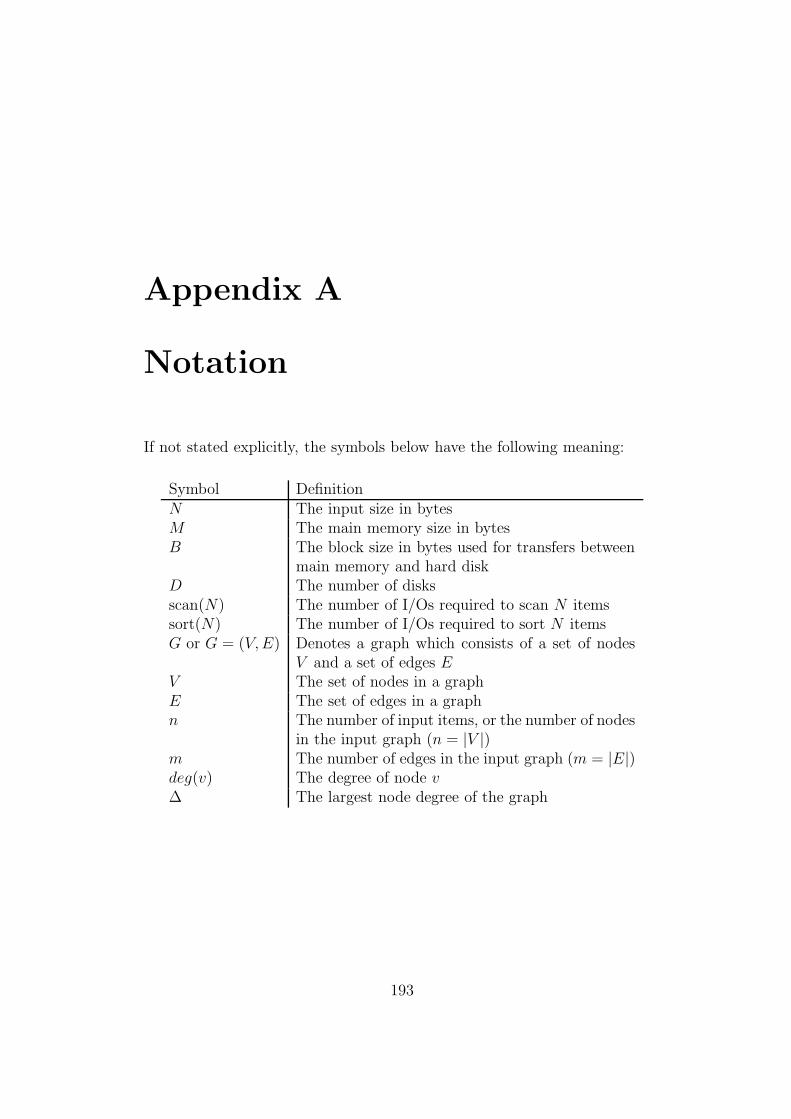
Appendix A
Notation
If not stated explicitly, the symbols below have the following meaning:
Symbol DefinitionN The input size in bytesM The main memory size in bytesB The block size in bytes used for transfers between
main memory and hard diskD The number of disksscan(N) The number of I/Os required to scan N itemssort(N) The number of I/Os required to sort N itemsG or G = (V, E) Denotes a graph which consists of a set of nodes
V and a set of edges EV The set of nodes in a graphE The set of edges in a graphn The number of input items, or the number of nodes
in the input graph (n = |V |)m The number of edges in the input graph (m = |E|)deg(v) The degree of node v∆ The largest node degree of the graph
193

![Engineering motif search for large graphs · PDF fileTight results Are tight algorithms useful, in practice? [here: practice ~ proof-of-concept algorithm engineering]](https://img.pdfslide.tips/doc/110x75/5a7885397f8b9ae91b8b7e7f/engineering-motif-search-for-large-graphs-results-are-tight-algorithms-useful-in.jpg)


![A sweep line algorithm for computing Voronoi diagram of circle … › ~deng › cg › project › 2003f › ... · 2014-02-22 · [1] Fortune, S., 1987. A sweepline algorithm for](https://img.pdfslide.tips/doc/110x75/5f1169200273b0207c355d3a/a-sweep-line-algorithm-for-computing-voronoi-diagram-of-circle-a-deng-a-cg.jpg)


![Polynomial time deterministic identity testing algorithm for … · 2020. 6. 16. · Polynomial time deterministic identity testing algorithm for S[3]PSP[2] circuits via Edelstein-Kelly](https://img.pdfslide.tips/doc/110x75/6149c34c12c9616cbc68f918/polynomial-time-deterministic-identity-testing-algorithm-for-2020-6-16-polynomial.jpg)


![Fundamentals of Algorithm Analysis Algorithm : Design & Analysis [Tutorial - 1]](https://img.pdfslide.tips/doc/110x75/5a4d1b527f8b9ab0599a8161/fundamentals-of-algorithm-analysis-algorithm-design-analysis-tutorial.jpg)