Embed Size (px)
Citation preview
Algorithmic Aspects of ComNets (WS 13/14): 01 – Introduction 1
Algorithmic Aspects of Communication Networks
Chapter 1Introduction
Short Recapitulation of Networking Basics
Packet Forwarding and Routing
Characterizing Traffic
Traffic Demand and Link Utilization
http://www.tu-ilmenau.de/fakia/aacn.htmlhttp://www.tu-ilmenau.de/fakia/aacn.html
Algorithmic Aspects of ComNets (WS 13/14): 01 – Introduction 2
Short Recap: World Wide Web
You already know from a basic networking class what happens whenyou enter http://www.tu-ilmenau.de into a Web browser
???

Algorithmic Aspects of ComNets (WS 13/14): 01 – Introduction 3
Short Recap: Telephony
Also, you have a basic understanding what happens when picking up a telephone and making a phone call
How to find the peer’s phone? How to transmit speech?
You are aware of the differences between transferring a Web pageand a phone call (and their implications):
Web: Bunch of data that has to be transmitted
Phone: Continuous flow of information, must arrive in time
?
Algorithmic Aspects of ComNets (WS 13/14): 01 – Introduction 4
Simplest Communication: Direct Physical Connection
Web example: Browser=client and serverSimplest case: directly connect them by a (pair of) cable
Server provides data, client consumes it
Telephony: Connect two telephones via a (pair of) cable
Client Server
Algorithmic Aspects of ComNets (WS 13/14): 01 – Introduction 5
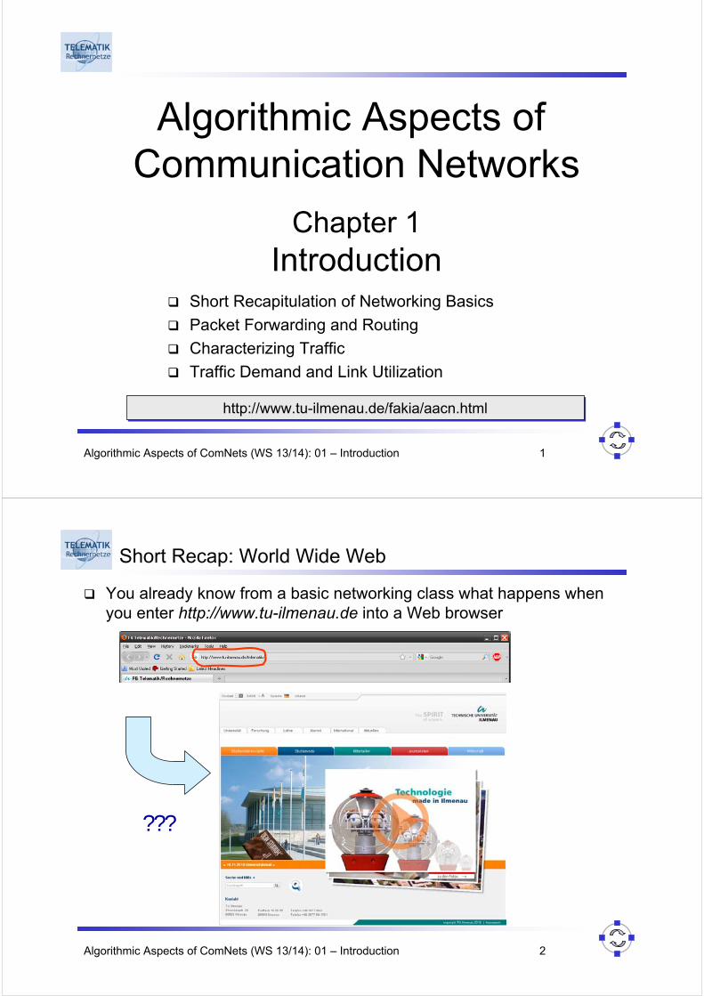
But There are More than Two Computers / Telephones
Connect each telephone / computer with each other one?
With four computers:
With eleven computers:
…
Algorithmic Aspects of ComNets (WS 13/14): 01 – Introduction 6
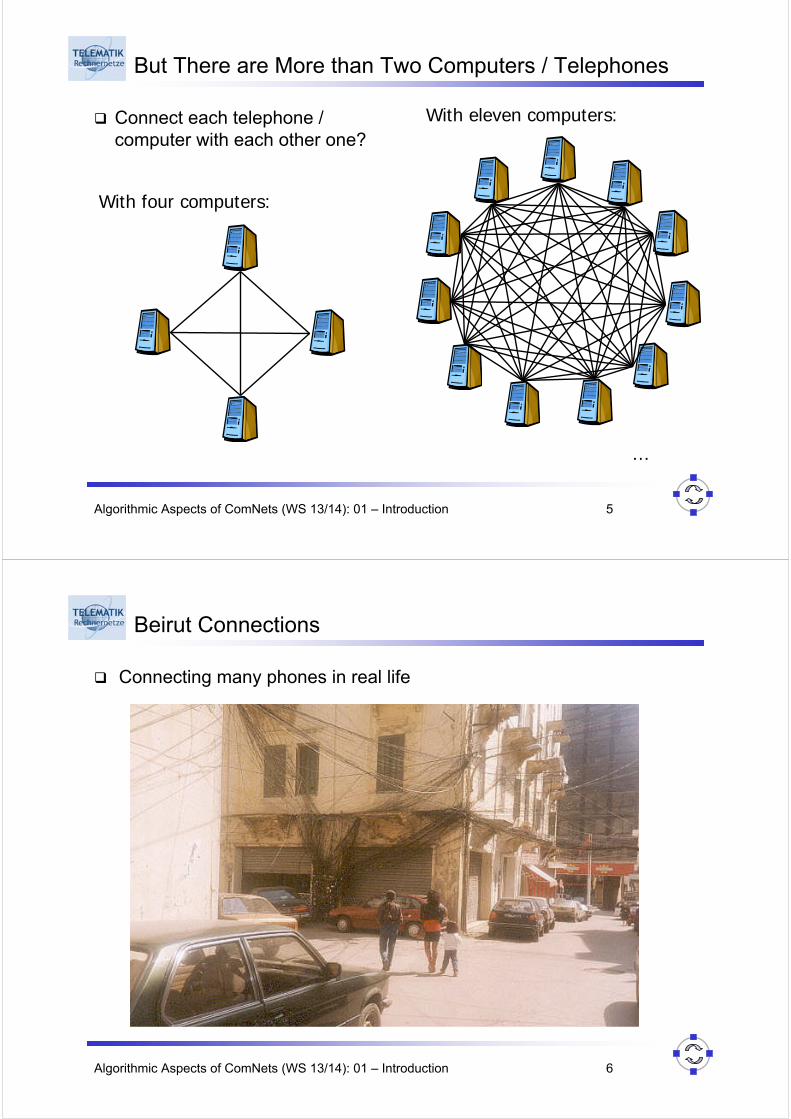
Beirut Connections
Connecting many phones in real life
Algorithmic Aspects of ComNets (WS 13/14): 01 – Introduction 7
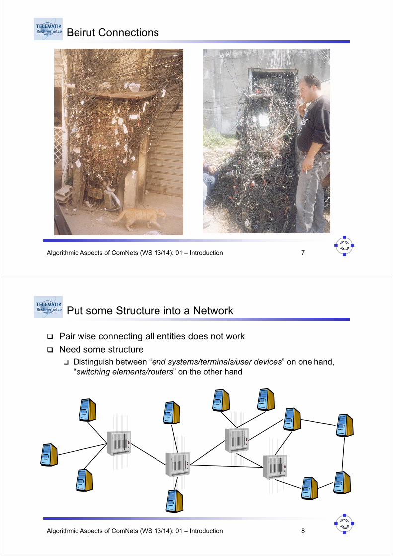
Beirut Connections
Algorithmic Aspects of ComNets (WS 13/14): 01 – Introduction 8
Put some Structure into a Network
Pair wise connecting all entities does not work
Need some structureDistinguish between “end systems/terminals/user devices” on one hand, “switching elements/routers” on the other hand
Algorithmic Aspects of ComNets (WS 13/14): 01 – Introduction 9
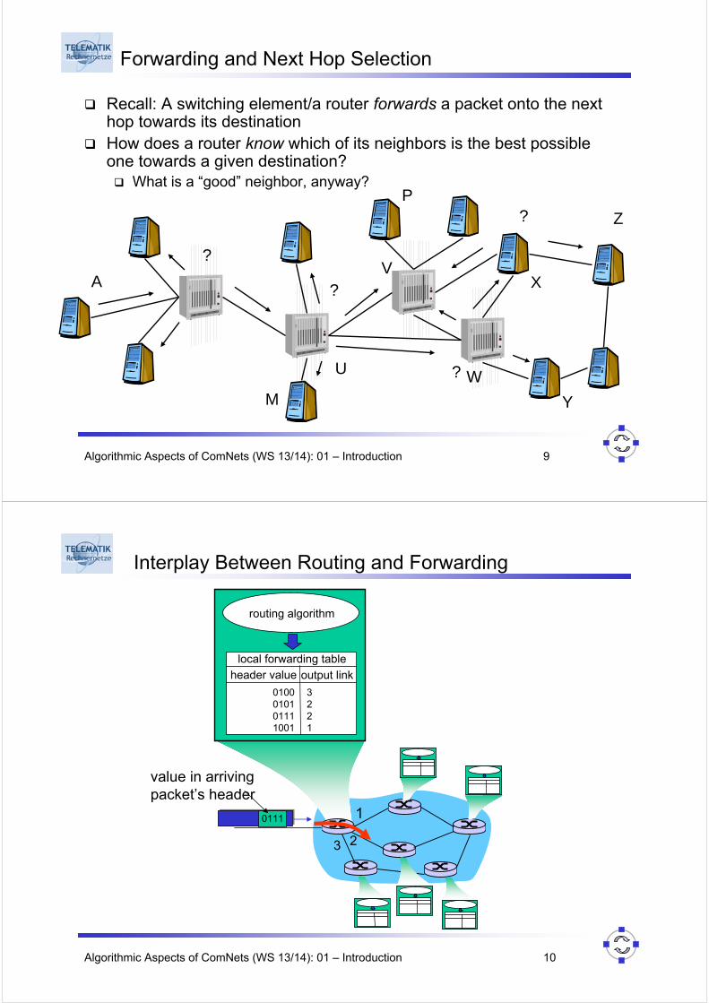
Forwarding and Next Hop Selection
Recall: A switching element/a router forwards a packet onto the next hop towards its destinationHow does a router know which of its neighbors is the best possible one towards a given destination?
What is a “good” neighbor, anyway?
A
Z
?
?
?
?
U
V
W
X
Y
P
M
Algorithmic Aspects of ComNets (WS 13/14): 01 – Introduction 10
1
23
0111
value in arrivingpacket’s header
routing algorithm
local forwarding tableheader value output link
0100010101111001
3221
Interplay Between Routing and Forwarding

Algorithmic Aspects of ComNets (WS 13/14): 01 – Introduction 11
Overview on Routing Algorithms (1)
An router executes a routing algorithm to decide which output line an incoming packet should be transmitted on:
In connection-oriented service, the routing algorithm is performed only during connection setup
In connectionless service, the routing algorithm is either performed as each packet arrives, or performed periodically and the results of this execution updated in the forwarding table
Often, routing algorithms take a so-called metric into account when making routing decisions:
In this context, a metric assigns a cost to each network link
This allows to compute a metric for each route in the network
A metric may take into account parameters like number of hops, “€ cost” of a link, delay, length of output queue, etc.
The “cheapest” path according to some metric is often also referred to as the shortest path (even though it might actually contain more hops than an alternative path)
Algorithmic Aspects of ComNets (WS 13/14): 01 – Introduction 12
Overview on Routing Algorithms (2)
Two basic types of routing algorithms:Non-adaptive routing algorithms: do not base their routing decisions on the current state of the network (example: flooding)
Adaptive routing algorithms: take into account the current network state when making routing decisions (examples: distance vector routing, link state routing)
Remark: additionally, hierarchical routing can be used to make these algorithms scale to large networks

Algorithmic Aspects of ComNets (WS 13/14): 01 – Introduction 13
Flooding
Basic strategy:Every incoming packet is sent out on every outgoing line except the one it arrived on
Problem: vast number of duplicated packets
Reducing the number of duplicated packets:Solution 1:
Have a hop counter in the packet header; routers decrement each arriving packet’s hop counter; routers discard a packet with hop count=0
Ideally, the hop counter should be initialized to the length of the path from the source to the destination
Solution 2:
Require the first router hop to put a sequence number in each packet it receives from its hosts
Each router maintains a table listing the sequence numbers it has seen from each first-hop router; the router can then discard packets it has already seen
Algorithmic Aspects of ComNets (WS 13/14): 01 – Introduction 14
Adaptive Routing Algorithms (1)
Problems with non-adaptive algorithms:If traffic levels in different parts of the subnet change dramatically and often, non-adaptive routing algorithms are unable to cope with these changes
Lots of computer traffic is bursty (~ very variable in intensity), but non-adaptive routing algorithms are usually based on average traffic conditions
Adaptive routing algorithms can deal with these situations
Three types:Centralized adaptive routing:
One central routing controller
Isolated adaptive routing:
Based on local information
Does not require exchange of information between routers
Distributed adaptive routing:
Routers periodically exchange information and compute updated routing information to be stored in their forwarding table
Algorithmic Aspects of ComNets (WS 13/14): 01 – Introduction 15
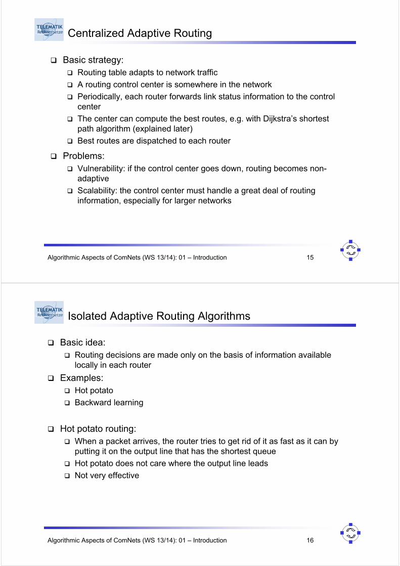
Centralized Adaptive Routing
Basic strategy:Routing table adapts to network traffic
A routing control center is somewhere in the network
Periodically, each router forwards link status information to the control center
The center can compute the best routes, e.g. with Dijkstra’s shortest path algorithm (explained later)
Best routes are dispatched to each router
Problems:Vulnerability: if the control center goes down, routing becomes non-adaptive
Scalability: the control center must handle a great deal of routing information, especially for larger networks
Algorithmic Aspects of ComNets (WS 13/14): 01 – Introduction 16
Isolated Adaptive Routing Algorithms
Basic idea: Routing decisions are made only on the basis of information available locally in each router
Examples:Hot potato
Backward learning
Hot potato routing:When a packet arrives, the router tries to get rid of it as fast as it can by putting it on the output line that has the shortest queue
Hot potato does not care where the output line leads
Not very effective

Algorithmic Aspects of ComNets (WS 13/14): 01 – Introduction 17
Backward Learning Routing
Basic idea:Packet headers include destination and source addresses; they also include a hop counter → learn from this data as packets pass by
Network nodes, initially ignorant of network topology, acquire knowledge of the network state as packets are handled
Algorithm:Routing is originally random (or hot potato, or flooding)
A packet with a hop count of one is from a directly connected node; thus, neighboring nodes are identified with their connecting links
A packet with a hop count of two is from a source two hops away, etc.
As packets arrive, the IMP compares the hop count for a given source address with the minimum hop count already registered; if the new one is less, it is substituted for the previous one
Remark: in order to be able to adapt to deterioration of routes (e.g. link failures) the acquired information has to be “forgotten” periodically
Algorithmic Aspects of ComNets (WS 13/14): 01 – Introduction 18
Distributed Adaptive Routing
Goal: Determine “good” path(sequence of routers) throughnetwork from source to dest.
Routing Protocol
A
ED
CB
F2
21
3
1
1
2
53
5
“Good” path:Typically means minimum cost path
Other definitions possible
Graph abstraction for routing algorithms:
Graph nodes are routers
Graph edges are physical linksLink cost: delay, $ cost, or congestion level
Path cost: sum of the link costs on the path
Algorithmic Aspects of ComNets (WS 13/14): 01 – Introduction 19
Decentralized Adaptive Routing Algorithm Classification
Global or decentralized information?
Decentralized:
Router knows physically-connectedneighbors, link costs to neighbors
Iterative process of computation,exchange of info with neighbors
“Distance vector” algorithms→ RIP protocol→ BGP protocol (“path vector”)
Global:
All routers have completetopology, link cost info
“Link state” algorithms→ Dijkstra’s algorithm→ OSPF protocol
Static or dynamic?
Static:
Routes change slowly over time
Dynamic:
Routes change more quickly
Periodic update
In response to link cost changes
Algorithmic Aspects of ComNets (WS 13/14): 01 – Introduction 20
Graph Model for Routing Algorithms (1)
Input: a graph G=(V, E) with
V = {v1, v2, …, vn} the set of nodes
E ⊆ V × V; E={e1, e2, …, em} the set of edges
A mapping c(vi, vj) representing the cost of edge (vi, vj) if (vi, vj) is in E(otherwise c(vi, vj) = infinity)
Start node s=vx an arbitrary node from the set V
Output: two arrays d and p with
d[i] containing the cost (distance) of the shortest path from s to vi
p[i] containing the index j of the predecessor node vj of vi on the shortest path from s to vi
Algorithmic Aspects of ComNets (WS 13/14): 01 – Introduction 21
Graph Model for Routing Algorithms (2)
Assumptions and Notation:Let s ∈ V be the source node
∀ v ∈ V: let δ(s, v) denote the cost of the shortest path from s to v
While d[i] denotes the shortest path cost (estimate) for node vi, we also write this as d(vi) in our proof later on
Assume that source node s is connected to every node v in the graph:
∀ s, v ∈ V: δ(s, v) < ∞Assume all edge weights are finite and positive:
∀ (v, w) ∈ E: c(v, w) > 0
Algorithmic Aspects of ComNets (WS 13/14): 01 – Introduction 22
Dijkstra‘s Algorithm for Shortest Paths (1)
Let us try to develop an algorithm for computing shortest paths by induction:
We could try induction on nodes or on edges: we choose nodes here
We need an estimate of costs to all nodes
Initially, this is set to infinity for all nodes except the source node s:∀ vi ∈ V \ {s}: d[i] := ∞
Cost estimate for node s=vx is set to 0: d[x] := 0
When trying to “reduce” our problem to a smaller one by making use of induction, it would not be wise to actually remove nodes from the graph, as this would change the graph (e.g. destroy connectivity)
Therefore, we run our induction on the number n of nodes for which we can compute the shortest paths
Base case: n = 1: We know how to compute the shortest path from s to s
Induction hypothesis: We know how to compute the lengths of the shortest paths and respective predecessor nodes for up to n nodes.

Algorithmic Aspects of ComNets (WS 13/14): 01 – Introduction 23
Dijkstra‘s Algorithm for Shortest Paths (2)
Induction step: n ⇝ n + 1Consider the set N of nodes for which we know the lengths of their shortest paths as well as the predecessor nodes:
Initially, N := {s}
So, we would like to increase the set N in every step by one node
But, which node of V \ N can be selected?
Clearly, it is not a good idea to choose a node vi for which our current shortest path cost estimate is high, e.g. d[i] = ∞
How to get better estimates?
Whenever we insert a node vi into N (also when s is inserted to N), we can update our estimates for nodes vj that are adjacent to vi: if ( d[i]+ c[i, j] < d[j]) {
d[j] = d[i] + c[i, j];p[j] = i; }
As d[i] is the cost of a path from s to vi, the cost of the shortest pathfrom s to vj can not be higher than d[i]+c[i, j]
Algorithmic Aspects of ComNets (WS 13/14): 01 – Introduction 24
Dijkstra‘s Algorithm for Shortest Paths (3)
Actually, we will show now by contradiction that in every step the vertex vi in V \ N with a minimal value d[i] can be inserted into N and that d[i] equals the shortest path cost from source s to vi (and at all subsequent times)
With this it is trivial to see that also the predecessor node is correctly set
Too see this, let us assume that this is not true when the n+1th node v is added to N
Thus the vertex v added has d(v) > δ (s, v)
Consider the situation just before insertion of v
Consider the true shortest path p from s to v (see next slide)
Algorithmic Aspects of ComNets (WS 13/14): 01 – Introduction 25
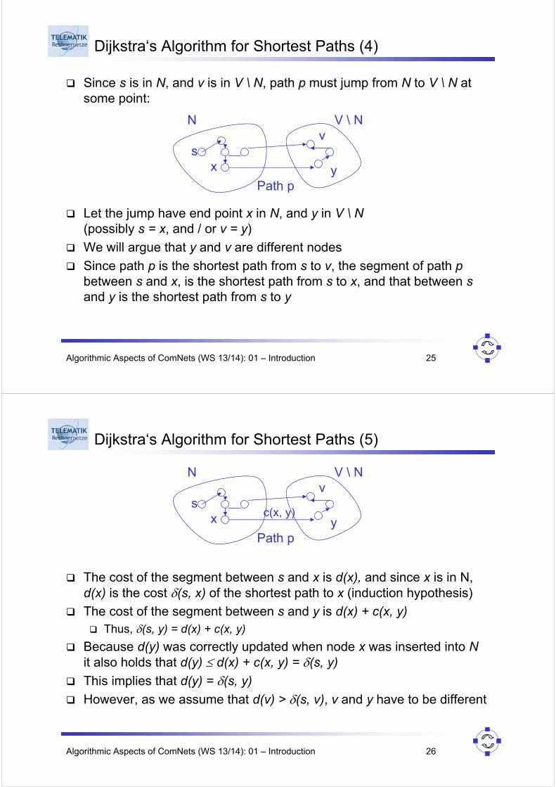
Dijkstra‘s Algorithm for Shortest Paths (4)
Since s is in N, and v is in V \ N, path p must jump from N to V \ N at some point:
N V \ N
sv
yx
Path p
Let the jump have end point x in N, and y in V \ N(possibly s = x, and / or v = y)
We will argue that y and v are different nodes
Since path p is the shortest path from s to v, the segment of path pbetween s and x, is the shortest path from s to x, and that between sand y is the shortest path from s to y
Algorithmic Aspects of ComNets (WS 13/14): 01 – Introduction 26
Dijkstra‘s Algorithm for Shortest Paths (5)
The cost of the segment between s and x is d(x), and since x is in N, d(x) is the cost δ(s, x) of the shortest path to x (induction hypothesis)
The cost of the segment between s and y is d(x) + c(x, y)Thus, δ(s, y) = d(x) + c(x, y)
Because d(y) was correctly updated when node x was inserted into Nit also holds that d(y) ≤ d(x) + c(x, y) = δ(s, y)
This implies that d(y) = δ(s, y)
However, as we assume that d(v) > δ(s, v), v and y have to be different
N V \ N
sv
yx
Path p
c(x, y)

Algorithmic Aspects of ComNets (WS 13/14): 01 – Introduction 27
Dijkstra‘s Algorithm for Shortest Paths (6)
Since y appears somewhere along the shortest path between s and v, but y and v are different, we can deduce that δ(s, y) < δ(s, v)
Here we use the assumption that all edges have positive cost
Hence, d(y) = δ(s, y) < δ(s, v) < d(v)
As both y and v are in V \ N, v can not have been chosen in this step, as the algorithm always chooses the node w with minimum d(w)
So, whenever a node v is included in N, it holds that d(v) = δ(s, v)
ys v
Algorithmic Aspects of ComNets (WS 13/14): 01 – Introduction 28
Dijkstra‘s Algorithm for Shortest Paths (7)
Termination of Dijkstra’s algorithm:As the algorithm adds one node to N in every step, the algorithm terminates when the costs of shortest paths to all nodes have been computed correctly
Algorithm complexity for |V| nodes:Each iteration: need to check all nodes v that are not yet in N
This requires |V|• (|V|+1)/2 comparisons, leading to O(|V|2)
This is optimal in dense graphs (where |E| ~ |V|2)
In sparse graphs, more efficient implementations are possible: O(|V|•log|V| + |E|) using so-called Fibonacci-heaps
Algorithmic Aspects of ComNets (WS 13/14): 01 – Introduction 29
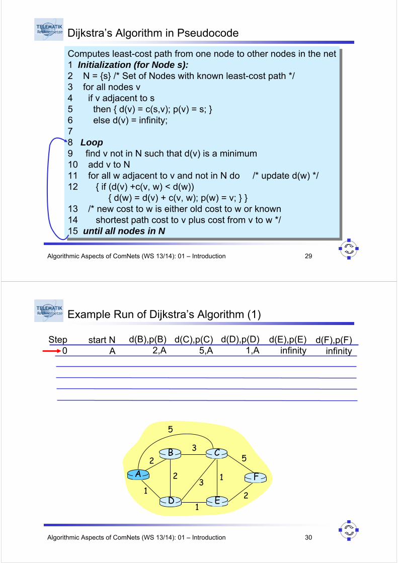
Dijkstra’s Algorithm in Pseudocode
Computes least-cost path from one node to other nodes in the net1 Initialization (for Node s):2 N = {s} /* Set of Nodes with known least-cost path */3 for all nodes v 4 if v adjacent to s 5 then { d(v) = c(s,v); p(v) = s; }6 else d(v) = infinity; 7 8 Loop9 find v not in N such that d(v) is a minimum 10 add v to N 11 for all w adjacent to v and not in N do /* update d(w) */12 { if (d(v) +c(v, w) < d(w))
{ d(w) = d(v) + c(v, w); p(w) = v; } }13 /* new cost to w is either old cost to w or known 14 shortest path cost to v plus cost from v to w */ 15 until all nodes in N
Algorithmic Aspects of ComNets (WS 13/14): 01 – Introduction 30
Example Run of Dijkstra’s Algorithm (1)
Step0
start NA
d(B),p(B)2,A
d(C),p(C)5,A
d(D),p(D)1,A
d(E),p(E)infinity
d(F),p(F)infinity
A
ED
CB
F2
2
13
1
1
2
53
5
Algorithmic Aspects of ComNets (WS 13/14): 01 – Introduction 31
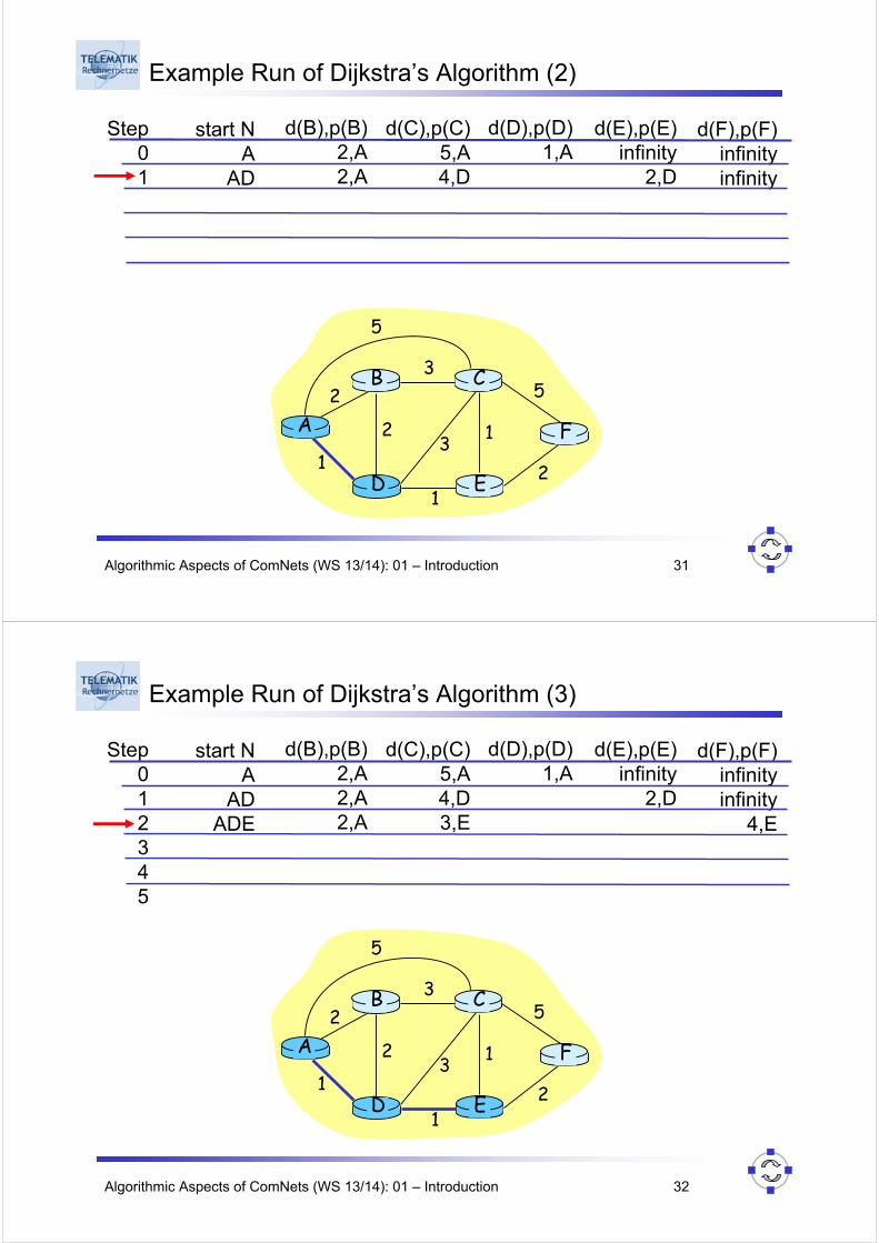
Example Run of Dijkstra’s Algorithm (2)
Step01
start NA
AD
d(B),p(B)2,A2,A
d(C),p(C)5,A4,D
d(D),p(D)1,A
d(E),p(E)infinity
2,D
d(F),p(F)infinityinfinity
A
ED
CB
F2
2
13
1
1
2
53
5
Algorithmic Aspects of ComNets (WS 13/14): 01 – Introduction 32
Example Run of Dijkstra’s Algorithm (3)
Step012345
start NA
ADADE
d(B),p(B)2,A2,A2,A
d(C),p(C)5,A4,D3,E
d(D),p(D)1,A
d(E),p(E)infinity
2,D
d(F),p(F)infinityinfinity
4,E
A
ED
CB
F2
2
13
1
1
2
53
5
Algorithmic Aspects of ComNets (WS 13/14): 01 – Introduction 33
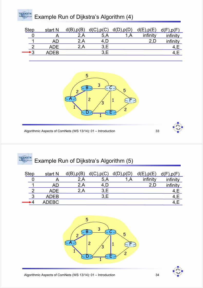
Example Run of Dijkstra’s Algorithm (4)
Step0123
start NA
ADADE
ADEB
d(B),p(B)2,A2,A2,A
d(C),p(C)5,A4,D3,E3,E
d(D),p(D)1,A
d(E),p(E)infinity
2,D
d(F),p(F)infinityinfinity
4,E4,E
A
ED
CB
F2
2
13
1
1
2
53
5
Algorithmic Aspects of ComNets (WS 13/14): 01 – Introduction 34
Example Run of Dijkstra’s Algorithm (5)
Step01234
start NA
ADADE
ADEBADEBC
d(B),p(B)2,A2,A2,A
d(C),p(C)5,A4,D3,E3,E
d(D),p(D)1,A
d(E),p(E)infinity
2,D
d(F),p(F)infinityinfinity
4,E4,E4,E
A
ED
CB
F2
2
13
1
1
2
53
5
Algorithmic Aspects of ComNets (WS 13/14): 01 – Introduction 35
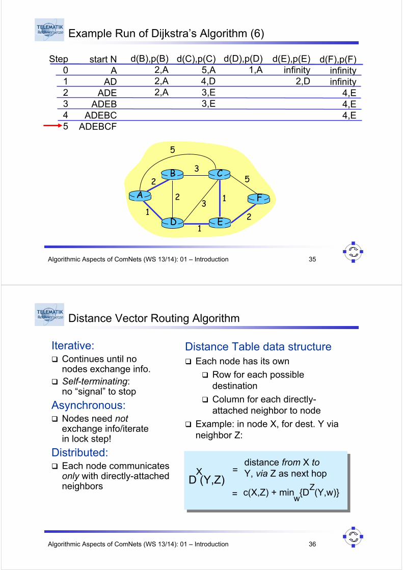
Example Run of Dijkstra’s Algorithm (6)
Step012345
start NA
ADADE
ADEBADEBC
ADEBCF
d(B),p(B)2,A2,A2,A
d(C),p(C)5,A4,D3,E3,E
d(D),p(D)1,A
d(E),p(E)infinity
2,D
d(F),p(F)infinityinfinity
4,E4,E4,E
A
ED
CB
F2
2
13
1
1
2
53
5
Algorithmic Aspects of ComNets (WS 13/14): 01 – Introduction 36
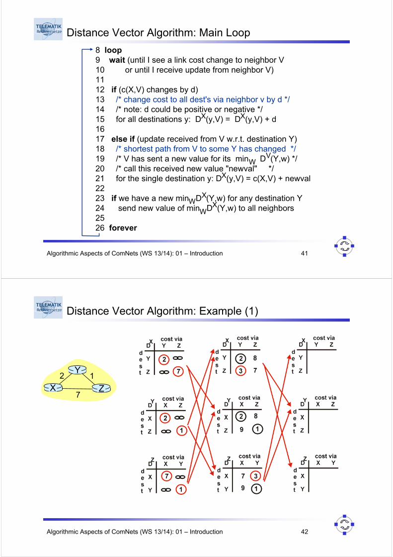
Distance Vector Routing Algorithm
Iterative:Continues until no nodes exchange info.Self-terminating: no “signal” to stop
Asynchronous:Nodes need notexchange info/iterate in lock step!
Distributed:Each node communicatesonly with directly-attachedneighbors
Distance Table data structureEach node has its own
Row for each possible destination
Column for each directly-attached neighbor to node
Example: in node X, for dest. Y vianeighbor Z:
D (Y,Z)X
distance from X toY, via Z as next hop
c(X,Z) + min {D (Y,w)}Z
w
=
=
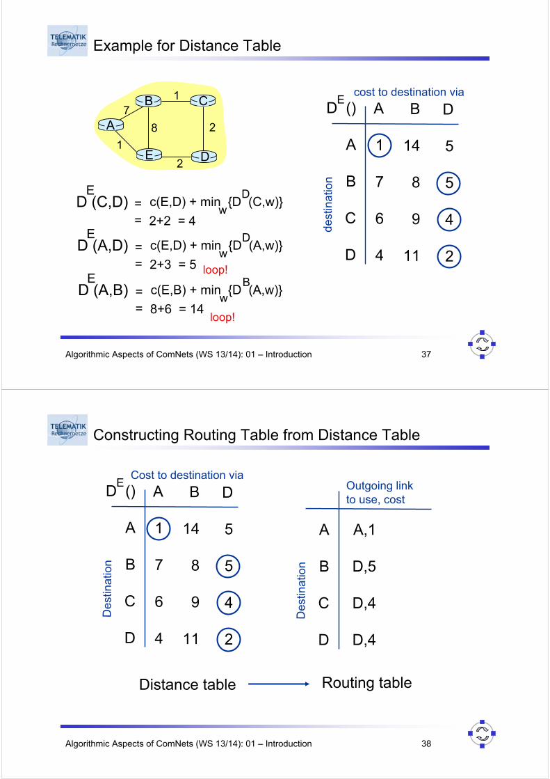
Algorithmic Aspects of ComNets (WS 13/14): 01 – Introduction 37
Example for Distance Table
A
E D
CB7
8
1
2
1
2
D ()
A
B
C
D
A
1
7
6
4
B
14
8
9
11
D
5
5
4
2
Ecost to destination via
dest
inat
ion
D (C,D)E
c(E,D) + min {D (C,w)}D
w== 2+2 = 4
D (A,D)E
c(E,D) + min {D (A,w)}D
w== 2+3 = 5
D (A,B)E
c(E,B) + min {D (A,w)}B
w== 8+6 = 14
loop!
loop!
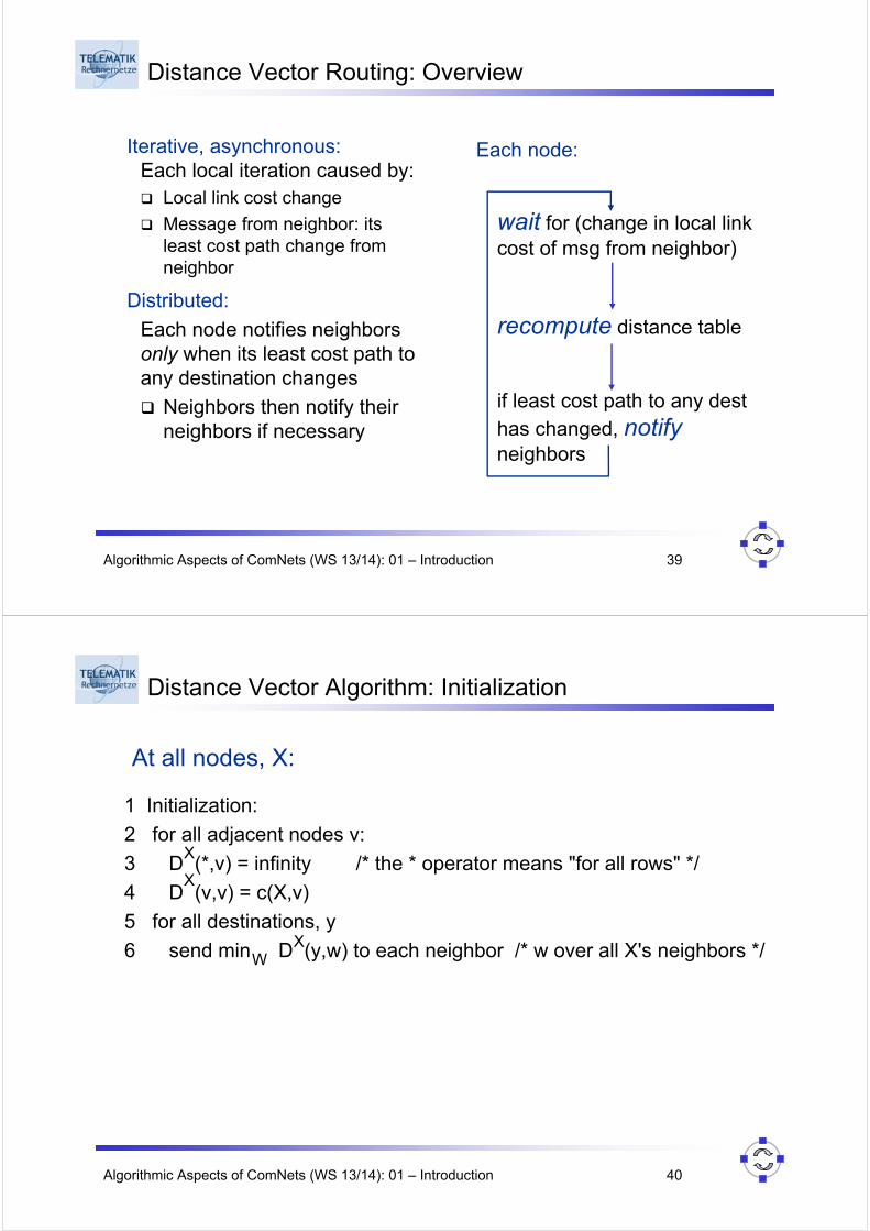
Algorithmic Aspects of ComNets (WS 13/14): 01 – Introduction 38
Constructing Routing Table from Distance Table
D ()
A
B
C
D
A
1
7
6
4
B
14
8
9
11
D
5
5
4
2
ECost to destination via
Des
tinat
ion
A
B
C
D
A,1
D,5
D,4
D,4
Outgoing link to use, cost
Des
tinat
ion
Distance table Routing table
Algorithmic Aspects of ComNets (WS 13/14): 01 – Introduction 39
Distance Vector Routing: Overview
Iterative, asynchronous:Each local iteration caused by:
Local link cost change
Message from neighbor: its least cost path change from neighbor
Distributed:
Each node notifies neighborsonly when its least cost path toany destination changes
Neighbors then notify their neighbors if necessary
wait for (change in local link cost of msg from neighbor)
recompute distance table
if least cost path to any desthas changed, notifyneighbors
Each node:
Algorithmic Aspects of ComNets (WS 13/14): 01 – Introduction 40
Distance Vector Algorithm: Initialization
1 Initialization:
2 for all adjacent nodes v:
3 D (*,v) = infinity /* the * operator means "for all rows" */
4 D (v,v) = c(X,v)
5 for all destinations, y
6 send min D (y,w) to each neighbor /* w over all X's neighbors */
At all nodes, X:
X
X
XW
Algorithmic Aspects of ComNets (WS 13/14): 01 – Introduction 41
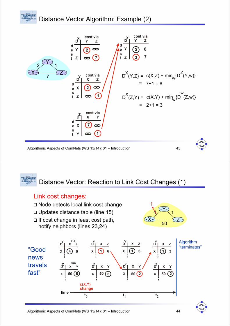
Distance Vector Algorithm: Main Loop
8 loop9 wait (until I see a link cost change to neighbor V 10 or until I receive update from neighbor V) 11 12 if (c(X,V) changes by d) 13 /* change cost to all dest's via neighbor v by d */ 14 /* note: d could be positive or negative */ 15 for all destinations y: D (y,V) = D (y,V) + d 16 17 else if (update received from V w.r.t. destination Y) 18 /* shortest path from V to some Y has changed */ 19 /* V has sent a new value for its min D (Y,w) */ 20 /* call this received new value "newval" */ 21 for the single destination y: D (y,V) = c(X,V) + newval22 23 if we have a new min D (Y,w) for any destination Y 24 send new value of min D (Y,w) to all neighbors 25 26 forever
X X
VW
X
XX
W
W
Algorithmic Aspects of ComNets (WS 13/14): 01 – Introduction 42
Distance Vector Algorithm: Example (1)
X Z
12
7
Y
Algorithmic Aspects of ComNets (WS 13/14): 01 – Introduction 43
Distance Vector Algorithm: Example (2)
X Z
12
7
Y
D (Y,Z)X
c(X,Z) + min {D (Y,w)}w=
= 7+1 = 8
Z
D (Z,Y)X
c(X,Y) + min {D (Z,w)}w=
= 2+1 = 3
Y
Algorithmic Aspects of ComNets (WS 13/14): 01 – Introduction 44
Distance Vector: Reaction to Link Cost Changes (1)
Link cost changes:Node detects local link cost change
Updates distance table (line 15)
If cost change in least cost path, notify neighbors (lines 23,24)
X Z
14
50
Y1
Algorithm“terminates”“Good
news travelsfast”

Algorithmic Aspects of ComNets (WS 13/14): 01 – Introduction 45
Distance Vector: Reaction to Link Cost Changes (2)
Link cost changes:Good news travels fast
Bad news travels slow -“count to infinity” problem!
algorithmcontinues
on!
X Z
14
50
Y60
Algorithmic Aspects of ComNets (WS 13/14): 01 – Introduction 46
Distance Vector: Poisoned Reverse
If Z routes through Y to get to X:
Z tells Y its (Z’s) distance to X is infinite (so Y won’t route to X via Z)
Will this completely solve count to infinityproblem?
algorithmterminates
X Z
14
50
Y60

Algorithmic Aspects of ComNets (WS 13/14): 01 – Introduction 47
The Bellman-Ford Algorithm (1)
In our correctness proof of Dijkstra’s algorithm, we assumed that all link costs are positive: ∀ (v, w) ∈ E: c(v, w) > 0
In fact, it is possible to proof that the algorithm also correctly computes the shortest path from s to all nodes v in case that link costs may be zero (see [CLR90, section 25.2])
The Bellman-Ford algorithm is capable of solving the even more general problem of computing shortest paths in graphs in which edges with negative cost exist:
In order for the shortest paths to be well defined in such graphs, it is required that there exist no negative weight cycles in the graph
Otherwise, the cost of the shortest path would “grow” to -∞ on a path with infinite length containing infinite many tours along one or more negative weight cycles
When being run on a graph G=(V, E) the algorithm detects, if there are negative weight cycles in G and computes the shortest paths from one source node s to all other nodes, in case that no such cycles exist
Algorithmic Aspects of ComNets (WS 13/14): 01 – Introduction 48
The Bellman-Ford Algorithm (2)
Why do we care about this algorithm at all, and why at this point of the lecture?
First, because we have to care about this algorithm, as it is the basis of distance vector routing
Second, because it is easier to understand its proof after having learned about Dijkstra’s algorithm
Like Dijkstra’s algorithm, the Bellman-Ford algorithm iteratively improves an estimate of the cost to reach each node:
The idea of the algorithm is to iterate |V|-1 times over all edges (u, v) ∈ E and check, if the current estimate for the node v can be improved by making use of edge (u, v) given the current estimate of the cost to reach node u
Compared with Dijkstra’s algorithm, which does not need to reconsider edges of nodes that have already been included in the set N, the Bellman-Ford algorithm always checks all edges, leading to a higher running time in the order of O(|V|•|E|)

Algorithmic Aspects of ComNets (WS 13/14): 01 – Introduction 49
The Bellman-Ford Algorithm (3)
Computes least-cost path from one node to other nodes in the net1 Initialization (for Node s):2 d(s) = 0;3 for all nodes v ≠ s { d(v) = infinity; p(v) = NULL; }4 Main Algorithm5 for i = 1 to |V| - 1 {6 for all edges (u, v) ∈ E { /* see if (u, v) can improve d(v) */7 if (d(u) +c(u, v) < d(v)) {8 d(v) = d(u) + c(u, v); p(v) = u; 9 } /* of <if (u, v) can improve current d(v) */10 } /* of <for all edges>11 } /* of <for i> */12 Check for negative cycles13 for all edges (u, v) ∈ E { /* see if (u, v) can still improve d(v) */14 if (d(u) +c(u, v) < d(v)) return FALSE;15 }16 return TRUE;
Computes least-cost path from one node to other nodes in the net1 Initialization (for Node s):2 d(s) = 0;3 for all nodes v ≠ s { d(v) = infinity; p(v) = NULL; }4 Main Algorithm5 for i = 1 to |V| - 1 {6 for all edges (u, v) ∈ E { /* see if (u, v) can improve d(v) */7 if (d(u) +c(u, v) < d(v)) {8 d(v) = d(u) + c(u, v); p(v) = u; 9 } /* of <if (u, v) can improve current d(v) */10 } /* of <for all edges>11 } /* of <for i> */12 Check for negative cycles13 for all edges (u, v) ∈ E { /* see if (u, v) can still improve d(v) */14 if (d(u) +c(u, v) < d(v)) return FALSE;15 }16 return TRUE;
Algorithmic Aspects of ComNets (WS 13/14): 01 – Introduction 50
The Bellman-Ford Algorithm (4)
Intuition behind the check for negative cycles:
In a graph with |V| nodes and no negative cycles, a shortest path from node s to any node v, can at most have |V|-1 edges
We will see, that after the i-th iteration, all lengths of shortest paths to nodes vi that are i hops away from s have been properly computed
Thus, after |V|-1 iterations, all shortest paths with a length of up to |V|-1 have been properly computed
So, if a further improvement is possible, this implies that the resulting path must have a length > |V|-1, and it can therefore be concluded that such a path must contain a negative cost cycle
Algorithmic Aspects of ComNets (WS 13/14): 01 – Introduction 51
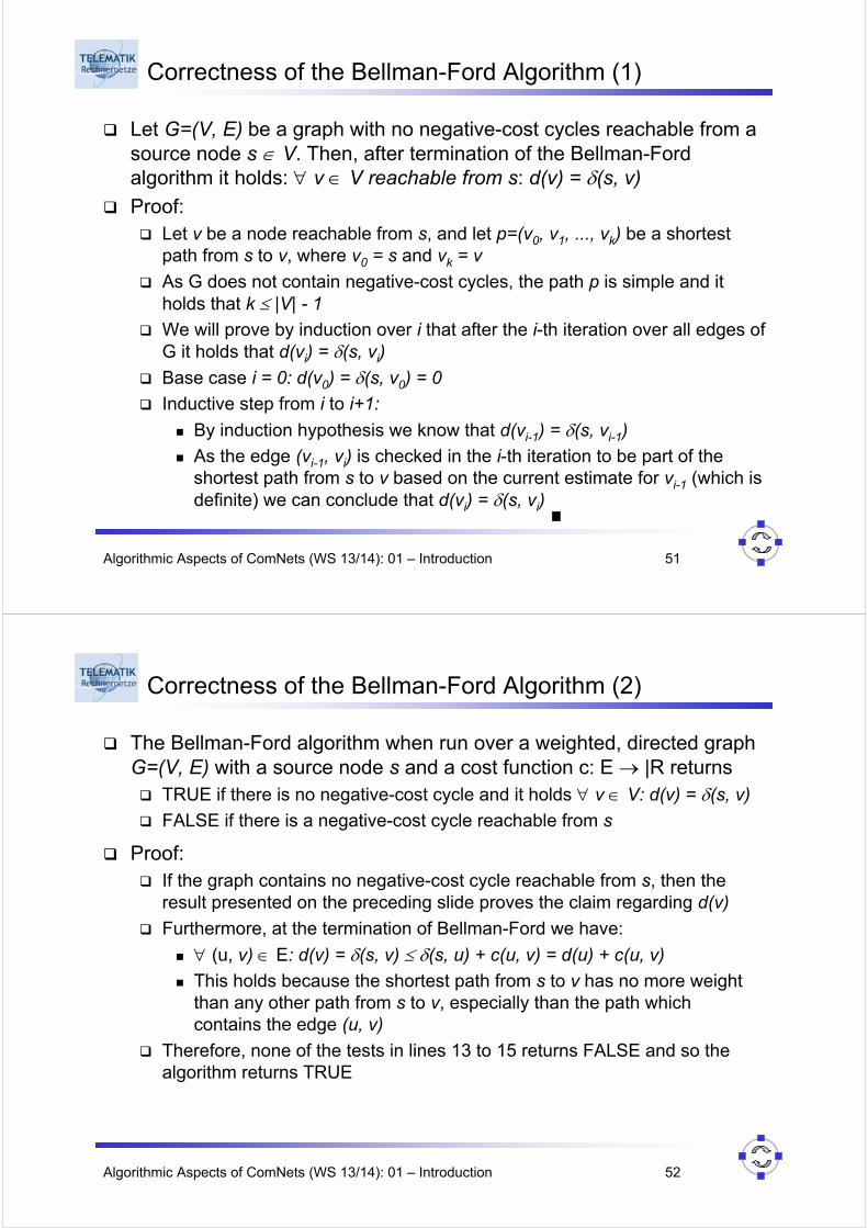
Correctness of the Bellman-Ford Algorithm (1)
Let G=(V, E) be a graph with no negative-cost cycles reachable from a source node s ∈ V. Then, after termination of the Bellman-Ford algorithm it holds: ∀ v ∈ V reachable from s: d(v) = δ(s, v)
Proof:Let v be a node reachable from s, and let p=(v0, v1, ..., vk) be a shortest path from s to v, where v0 = s and vk = v
As G does not contain negative-cost cycles, the path p is simple and it holds that k ≤ |V| - 1
We will prove by induction over i that after the i-th iteration over all edges of G it holds that d(vi) = δ(s, vi)
Base case i = 0: d(v0) = δ(s, v0) = 0
Inductive step from i to i+1:
By induction hypothesis we know that d(vi-1) = δ(s, vi-1)
As the edge (vi-1, vi) is checked in the i-th iteration to be part of the shortest path from s to v based on the current estimate for vi-1 (which is definite) we can conclude that d(vi) = δ(s, vi)
Algorithmic Aspects of ComNets (WS 13/14): 01 – Introduction 52
Correctness of the Bellman-Ford Algorithm (2)
The Bellman-Ford algorithm when run over a weighted, directed graph G=(V, E) with a source node s and a cost function c: E → |R returns
TRUE if there is no negative-cost cycle and it holds ∀ v ∈ V: d(v) = δ(s, v)
FALSE if there is a negative-cost cycle reachable from s
Proof:If the graph contains no negative-cost cycle reachable from s, then the result presented on the preceding slide proves the claim regarding d(v)
Furthermore, at the termination of Bellman-Ford we have:
∀ (u, v) ∈ E: d(v) = δ(s, v) ≤ δ(s, u) + c(u, v) = d(u) + c(u, v)
This holds because the shortest path from s to v has no more weight than any other path from s to v, especially than the path which contains the edge (u, v)
Therefore, none of the tests in lines 13 to 15 returns FALSE and so the algorithm returns TRUE
Algorithmic Aspects of ComNets (WS 13/14): 01 – Introduction 53
Correctness of the Bellman-Ford Algorithm (3)
Let us now assume that G contains a negative-cost cycle reachable from s:
Let z = (v0, v1, ..., vk) be the negative-cost cycle with v0, = vk
Thus it holds that
Let us assume, that the algorithm returns TRUE
In this case, we have ∀ i ∈ {1, ..., k}: d(vi) ≤ d(vi-1) + c(vi-1, vi)
Summing the equalities around the cycle z leads to
Since each link appears only once in the cycle z, it holds
and we have
which contradicts the above inequality
Thus, the algorithm returns FALSE
0),(1
1 <∑=
−
k
iii vvc
∑∑∑=
−=
−=
+≤k
iii
k
ii
k
ii vvcvdvd
11
11
1
),()()(
∑∑=
−=
=k
ii
k
ii vdvd
11
1
)()(
∑=
−≤k
iii vvc
11 ),(0
0),(1
1 <∑=
−
k
iii vvc
Algorithmic Aspects of ComNets (WS 13/14): 01 – Introduction 54
Comparison of Link State and Distance Vector Algorithms
Message complexityLS: with n nodes, E links,
O(n•E) msgs sent each DV: exchange between
neighbors onlyconvergence time varies
Speed of ConvergenceLS: O(n2) algorithm requires
O(n•E) msgsmay have oscillations
DV: convergence time variesmay be routing loopscount-to-infinity problem
Robustness: what happens if router malfunctions?LS:
Node can advertise incorrect link costEach node computes only its own table
DV:DV node can advertise incorrect path costEach node’s table used by other routers:
Errors propagate through network
Algorithmic Aspects of ComNets (WS 13/14): 01 – Introduction 55
Hierarchical Routing
Scale (>100 million destinations!):Can’t store all destinations inrouting tablesRouting table exchangewould overload links
Administrative autonomy:
Internet = network of networks
Each network admin may wantto control routing in its ownnetwork
Our routing study so far is an idealization:
All routers are assumed to be identical
Network is assumed to be “flat”
… Practice, however, looks different
Algorithmic Aspects of ComNets (WS 13/14): 01 – Introduction 56
Data Transmission in Interconnected Networks
Data transmission usually involves multiple networks
Routing in Internet distinguishes two levels:Intradomain routing inside autonomous systems (networks themselves)
Interdomain routing between autonomous systems (AS)
Internet-wide routing via border gateway protocol (BGP) operates on the AS level, every intermediate network is considered as being one hop
Internet service providers (ISP) have peering agreements & “links”If no direct link is possible, ISPs connect via a transport provider network
Algorithmic Aspects of ComNets (WS 13/14): 01 – Introduction 57
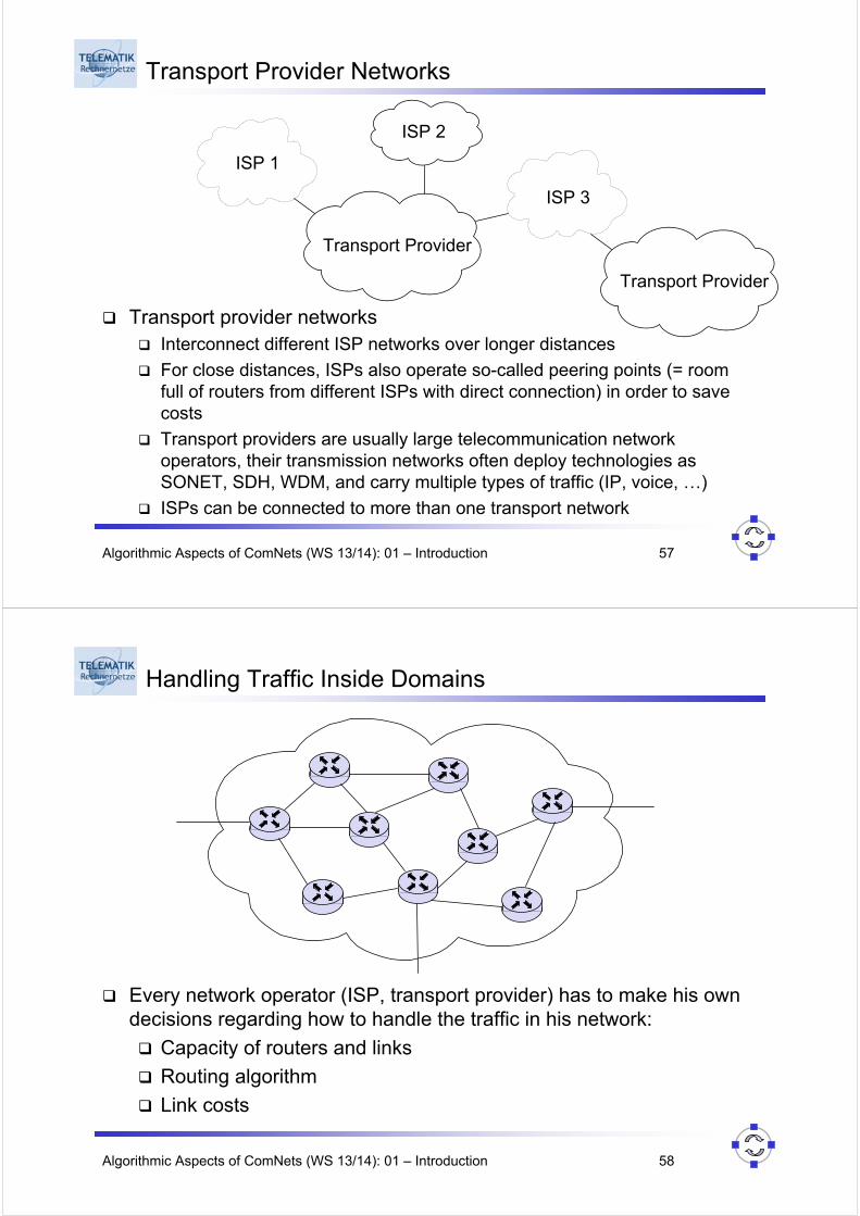
Transport Provider Networks
Transport provider networks Interconnect different ISP networks over longer distances
For close distances, ISPs also operate so-called peering points (= room full of routers from different ISPs with direct connection) in order to save costs
Transport providers are usually large telecommunication network operators, their transmission networks often deploy technologies as SONET, SDH, WDM, and carry multiple types of traffic (IP, voice, …)
ISPs can be connected to more than one transport network
Transport Provider
ISP 1
ISP 2
ISP 3
Transport Provider
Algorithmic Aspects of ComNets (WS 13/14): 01 – Introduction 58
Handling Traffic Inside Domains
Every network operator (ISP, transport provider) has to make his own decisions regarding how to handle the traffic in his network:
Capacity of routers and links
Routing algorithm
Link costs
Algorithmic Aspects of ComNets (WS 13/14): 01 – Introduction 59
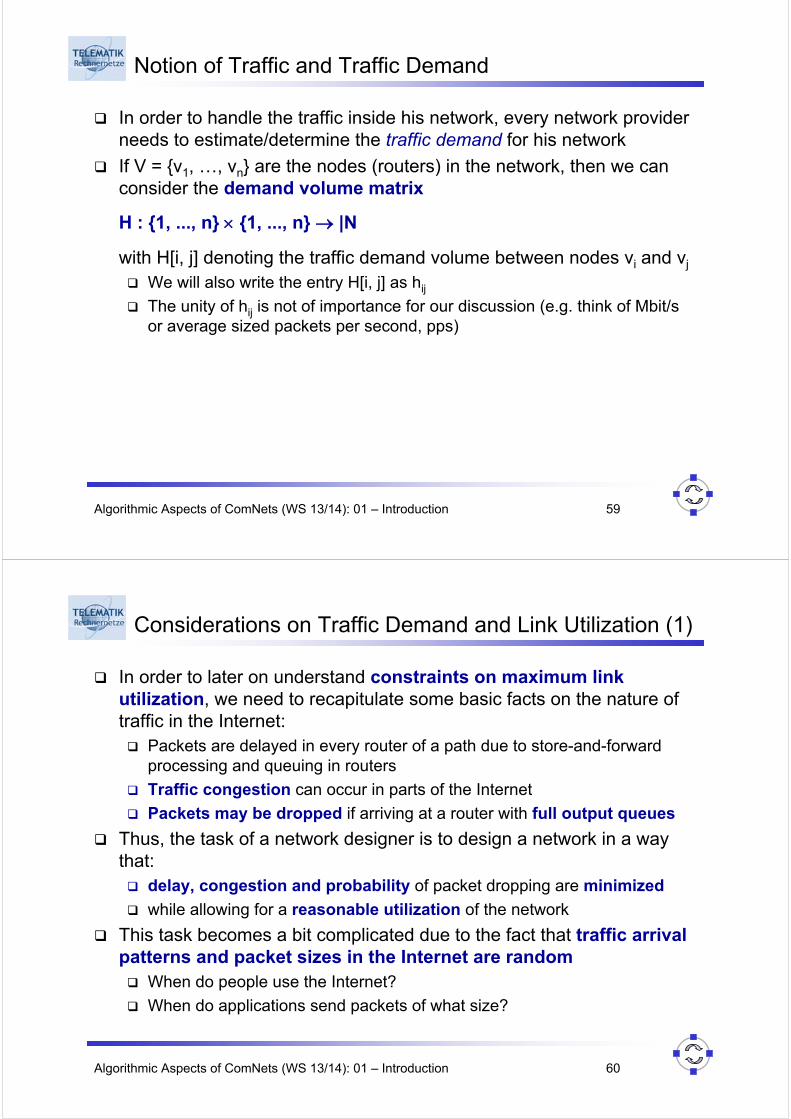
Notion of Traffic and Traffic Demand
In order to handle the traffic inside his network, every network provider needs to estimate/determine the traffic demand for his network
If V = {v1, …, vn} are the nodes (routers) in the network, then we can consider the demand volume matrix
H : {1, ..., n} × {1, ..., n} → |N
with H[i, j] denoting the traffic demand volume between nodes vi and vj
We will also write the entry H[i, j] as hij
The unity of hij is not of importance for our discussion (e.g. think of Mbit/sor average sized packets per second, pps)
Algorithmic Aspects of ComNets (WS 13/14): 01 – Introduction 60
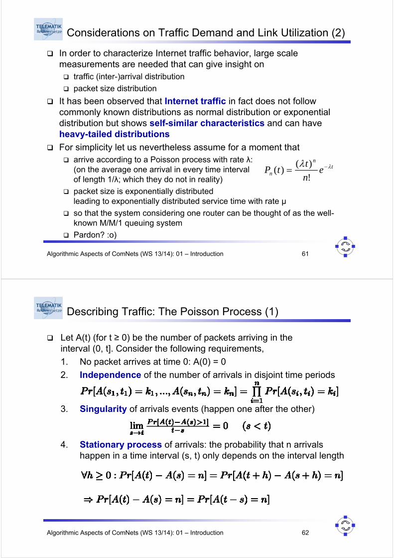
Considerations on Traffic Demand and Link Utilization (1)
In order to later on understand constraints on maximum link utilization, we need to recapitulate some basic facts on the nature of traffic in the Internet:
Packets are delayed in every router of a path due to store-and-forward processing and queuing in routers
Traffic congestion can occur in parts of the Internet
Packets may be dropped if arriving at a router with full output queues
Thus, the task of a network designer is to design a network in a way that:
delay, congestion and probability of packet dropping are minimized
while allowing for a reasonable utilization of the network
This task becomes a bit complicated due to the fact that traffic arrival patterns and packet sizes in the Internet are random
When do people use the Internet?
When do applications send packets of what size?
Algorithmic Aspects of ComNets (WS 13/14): 01 – Introduction 61
Considerations on Traffic Demand and Link Utilization (2)
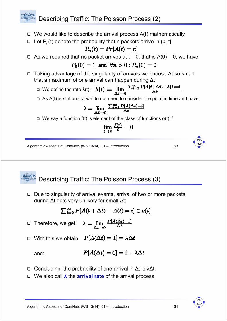
In order to characterize Internet traffic behavior, large scale measurements are needed that can give insight on
traffic (inter-)arrival distribution
packet size distribution
It has been observed that Internet traffic in fact does not follow commonly known distributions as normal distribution or exponential distribution but shows self-similar characteristics and can have heavy-tailed distributions
For simplicity let us nevertheless assume for a moment that arrive according to a Poisson process with rate λ: (on the average one arrival in every time interval of length 1/λ; which they do not in reality)
packet size is exponentially distributed leading to exponentially distributed service time with rate μ
so that the system considering one router can be thought of as the well-known M/M/1 queuing system
Pardon? :o)
tn
n en
ttP λλ −=
!
)()(
Algorithmic Aspects of ComNets (WS 13/14): 01 – Introduction 62
Describing Traffic: The Poisson Process (1)
Let A(t) (for t ≥ 0) be the number of packets arriving in the interval (0, t]. Consider the following requirements,
1. No packet arrives at time 0: A(0) = 0
2. Independence of the number of arrivals in disjoint time periods
3. Singularity of arrivals events (happen one after the other)
4. Stationary process of arrivals: the probability that n arrivalshappen in a time interval (s, t) only depends on the interval length
Algorithmic Aspects of ComNets (WS 13/14): 01 – Introduction 63
Describing Traffic: The Poisson Process (2)
We would like to describe the arrival process A(t) mathematically
Let Pn(t) denote the probability that n packets arrive in (0, t]
As we required that no packet arrives at t = 0, that is A(0) = 0, we have
Taking advantage of the singularity of arrivals we choose ∆t so small that a maximum of one arrival can happen during ∆t
We define the rate λ(t):
As A(t) is stationary, we do not need to consider the point in time and have
We say a function f(t) is element of the class of functions o(t) if
Algorithmic Aspects of ComNets (WS 13/14): 01 – Introduction 64
Describing Traffic: The Poisson Process (3)
Due to singularity of arrival events, arrival of two or more packets during ∆t gets very unlikely for small ∆t:
Therefore, we get:
With this we obtain:
and:
Concluding, the probability of one arrival in ∆t is λ∆t.
We also call λ the arrival rate of the arrival process.
Algorithmic Aspects of ComNets (WS 13/14): 01 – Introduction 65
Describing Traffic: The Poisson Process (4)
We would like to use this to compute the probability of having n > 0 arrivals in the interval (0, t + ∆t]
For this, we partition the interval into two intervals (0, t] and (t, t + ∆t]
We have to distinguish two cases that both may lead to n arrivals:We have n - 1 arrivals in interval (0, t] and one arrival in (t, ∆t]
We have n arrivals in interval (0, t] and no arrival in (t, ∆t]
t
t
0 t + ∆t
∆t
or
eithern - 1
n
1
0
Algorithmic Aspects of ComNets (WS 13/14): 01 – Introduction 66
Describing Traffic: The Poisson Process (5)
Both cases correspond to disjoint random events and there are nomore possibilities to have n arrivals in the interval (0, t + ∆t]
Thus
Due to independence and stationarity of the arrival process, we can simplify
Algorithmic Aspects of ComNets (WS 13/14): 01 – Introduction 67
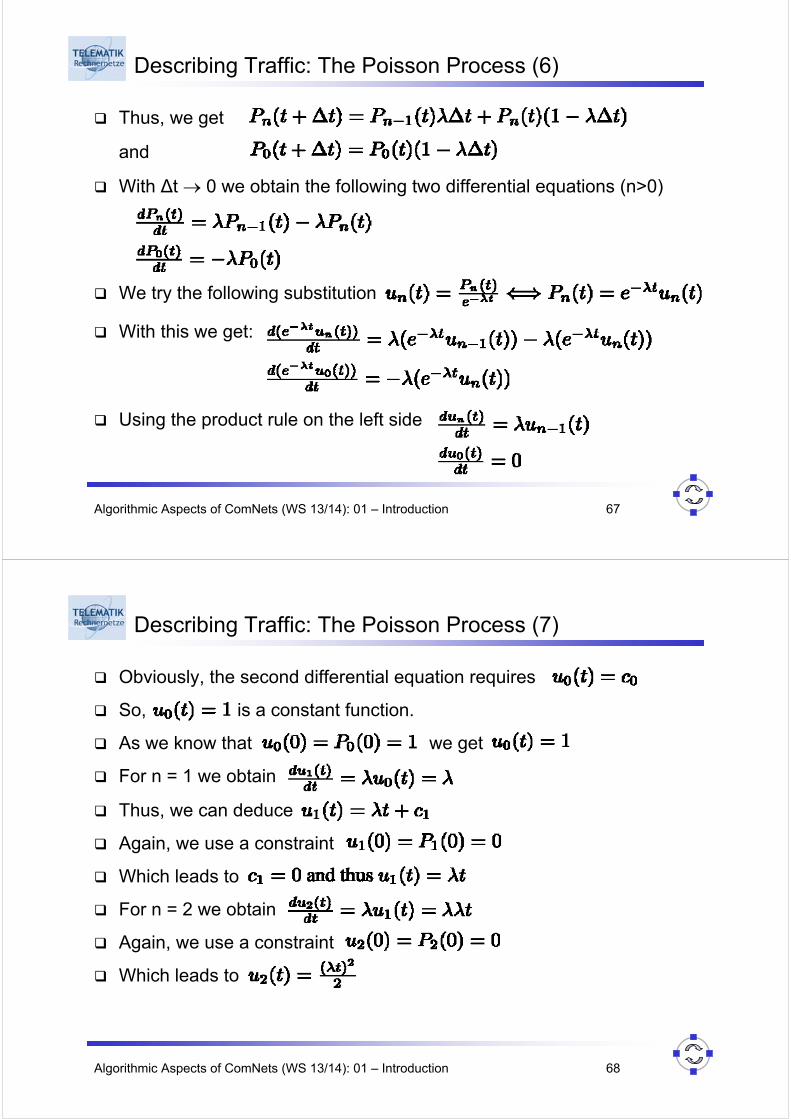
Describing Traffic: The Poisson Process (6)
Thus, we get
and
With ∆t → 0 we obtain the following two differential equations (n>0)
We try the following substitution
With this we get:
Using the product rule on the left side
Algorithmic Aspects of ComNets (WS 13/14): 01 – Introduction 68
Describing Traffic: The Poisson Process (7)
Obviously, the second differential equation requires
So, is a constant function.
As we know that we get
For n = 1 we obtain
Thus, we can deduce
Again, we use a constraint
Which leads to
For n = 2 we obtain
Again, we use a constraint
Which leads to
Algorithmic Aspects of ComNets (WS 13/14): 01 – Introduction 69
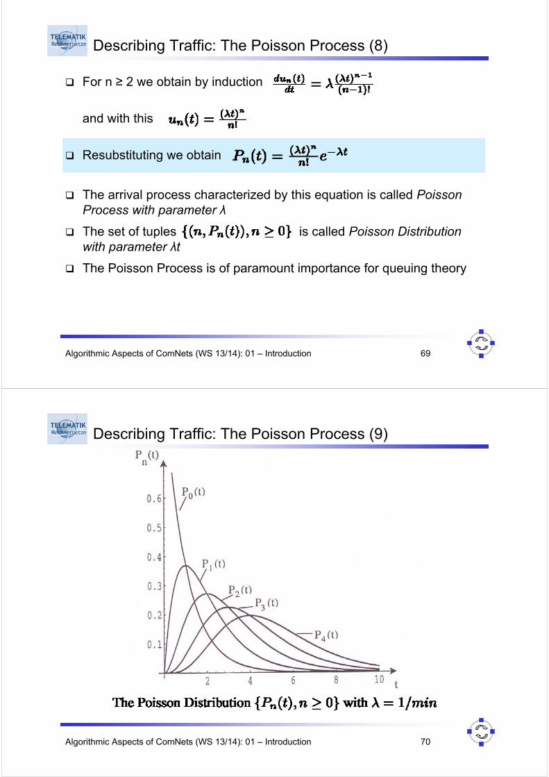
Describing Traffic: The Poisson Process (8)
For n ≥ 2 we obtain by induction
and with this
Resubstituting we obtain
The arrival process characterized by this equation is called Poisson Process with parameter λ
The set of tuples is called Poisson Distribution with parameter λt
The Poisson Process is of paramount importance for queuing theory
Algorithmic Aspects of ComNets (WS 13/14): 01 – Introduction 70
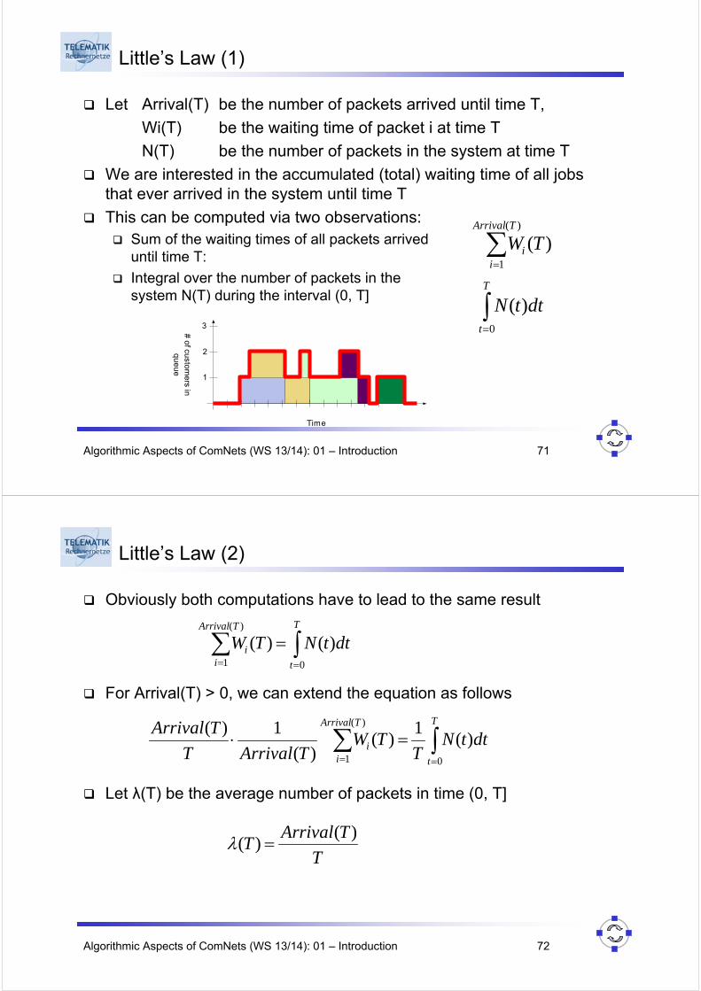
Describing Traffic: The Poisson Process (9)
Algorithmic Aspects of ComNets (WS 13/14): 01 – Introduction 71
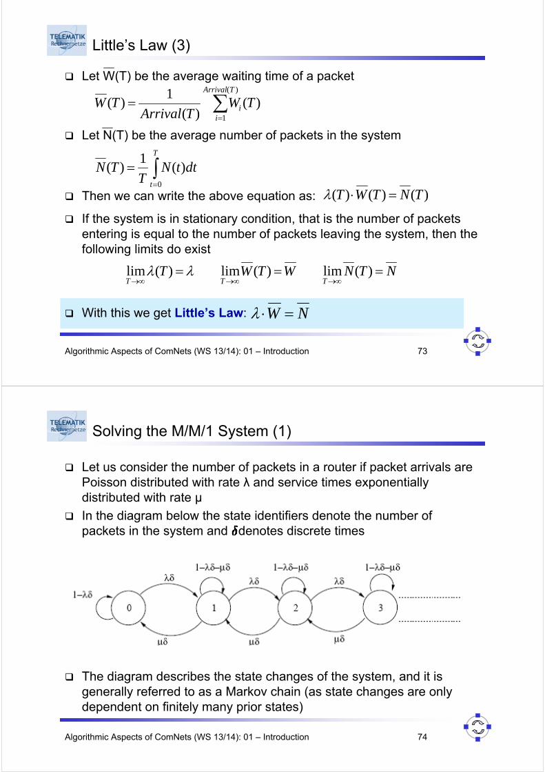
Little’s Law (1)
Let Arrival(T) be the number of packets arrived until time T,
Wi(T) be the waiting time of packet i at time T
N(T) be the number of packets in the system at time T
We are interested in the accumulated (total) waiting time of all jobs that ever arrived in the system until time T
This can be computed via two observations:Sum of the waiting times of all packets arrived until time T:
Integral over the number of packets in the system N(T) during the interval (0, T]
∑=
)(
1
)(TArrival
ii TW
∫=
T
t
dttN0
)(
# o
f custo
me
rs inq
ue
ue
Time
1
2
3
Algorithmic Aspects of ComNets (WS 13/14): 01 – Introduction 72
Little’s Law (2)
Obviously both computations have to lead to the same result
For Arrival(T) > 0, we can extend the equation as follows
Let λ(T) be the average number of packets in time (0, T]
∫∑==
=T
t
TArrival
ii dttNTW
0
)(
1
)()(
∫∑==
=⋅T
t
TArrival
ii dttN
TTW
TArrivalT
TArrival
0
)(
1
)(1
)()(
1)(
T
TArrivalT
)()( =λ
Algorithmic Aspects of ComNets (WS 13/14): 01 – Introduction 73
Little’s Law (3)
Let W(T) be the average waiting time of a packet
Let N(T) be the average number of packets in the system
Then we can write the above equation as:
If the system is in stationary condition, that is the number of packets entering is equal to the number of packets leaving the system, then the following limits do exist
With this we get Little’s Law:
∑=
=)(
1
)()(
1)(
TArrival
ii TW
TArrivalTW
∫=
=T
t
dttNT
TN0
)(1
)(
)()()( TNTWT =⋅λ
NTNWTWTTTT
===∞→∞→∞→
)(lim)(lim)(lim λλ
NW =⋅λ
Algorithmic Aspects of ComNets (WS 13/14): 01 – Introduction 74
Solving the M/M/1 System (1)
Let us consider the number of packets in a router if packet arrivals are Poisson distributed with rate λ and service times exponentially distributed with rate μ
In the diagram below the state identifiers denote the number of packets in the system and denotes discrete times
The diagram describes the state changes of the system, and it isgenerally referred to as a Markov chain (as state changes are only dependent on finitely many prior states)

Algorithmic Aspects of ComNets (WS 13/14): 01 – Introduction 75
Solving the M/M/1 System (2)
Let pn denote the probability of the system being in state n
Then in case of statistical balance between states, we can formulate
the following equation for all states n:
Recall: (geometric sum)
As furthermore,
we obtain
(this also holds if we consider )
Algorithmic Aspects of ComNets (WS 13/14): 01 – Introduction 76
Solving the M/M/1 System (3)
Let us now consider the average number N of packets in the system
As Little’s Law states
we obtain for the average waiting time
Note that with we will have
Let us resume our considerations on traffic demand and link utilization
and
Algorithmic Aspects of ComNets (WS 13/14): 01 – Introduction 77
Considerations on Traffic Demand and Link Utilization (3)
If packets have average size Kp bits and link capacity is C bits per second then the average service rate of the link is μp = C / Kp pps(packets per second)
If the average arrival rate is λp pps then the average delay is given by
Even if vastly simplified (due to our simple traffic assumptions), this can provide useful insights on delay
Consider a T1-link with 1.54 Mbit/s, then for an average packet size of 1 kByte = 8 kbit the average service rate of the link is 190 pps
If the packets arrive with rate λp=100 pps, then the average delay is 1 / 90 ~ 11.11 ms
If the arrival rate is increased to 150 pps, the delay increases to 25 ms
Let us also consider the average link utilization ρ = λp / μp
For λp = 100 pps and μp = 190 pps, we have ρ = 0.526
( )pp
ppDλμ
μλ−
=1
,
Algorithmic Aspects of ComNets (WS 13/14): 01 – Introduction 78
Considerations on Traffic Demand and Link Utilization (4)
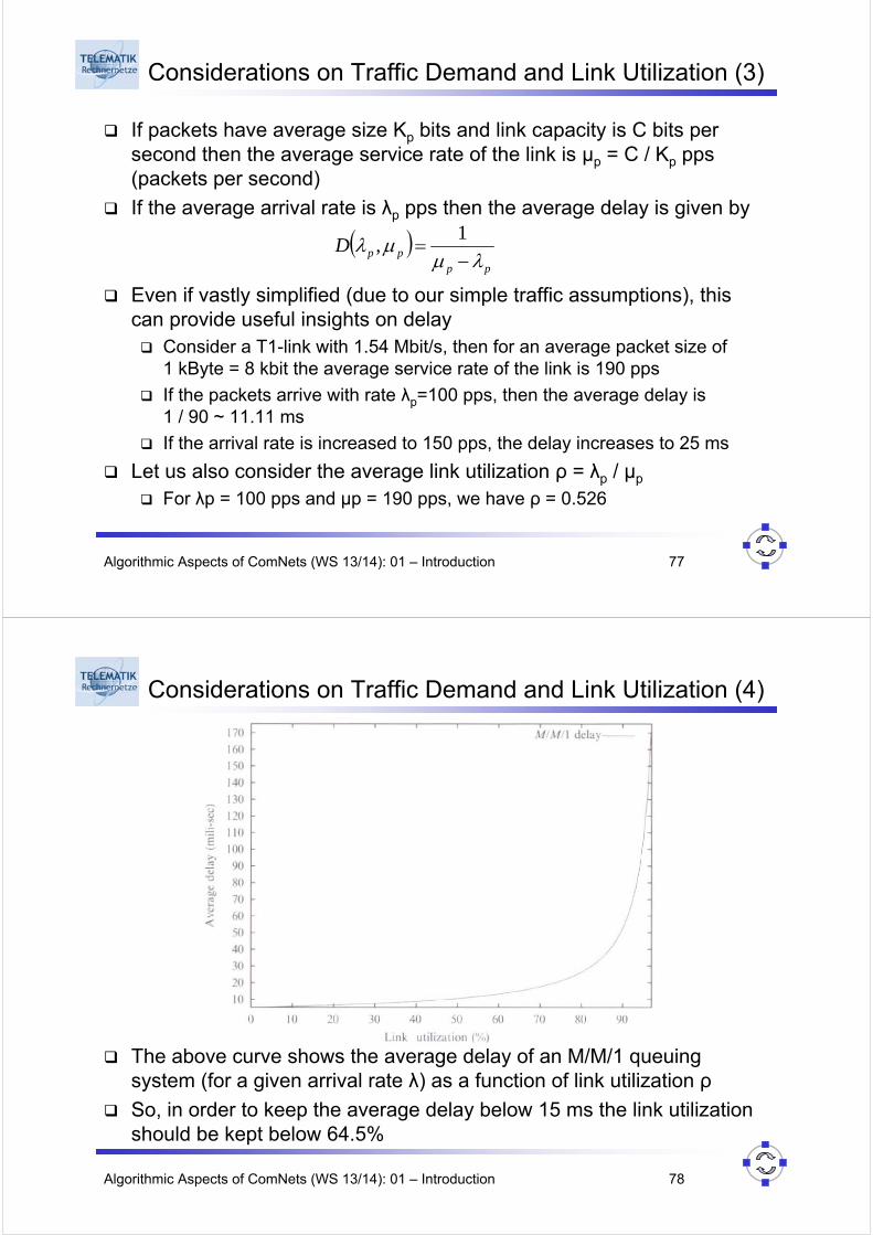
The above curve shows the average delay of an M/M/1 queuing system (for a given arrival rate λ) as a function of link utilization ρ
So, in order to keep the average delay below 15 ms the link utilization should be kept below 64.5%
Algorithmic Aspects of ComNets (WS 13/14): 01 – Introduction 79
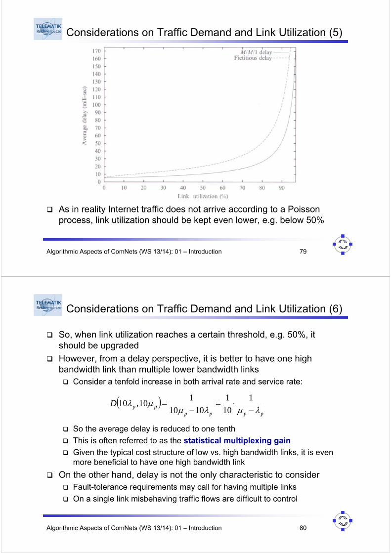
Considerations on Traffic Demand and Link Utilization (5)
As in reality Internet traffic does not arrive according to a Poisson process, link utilization should be kept even lower, e.g. below 50%
Algorithmic Aspects of ComNets (WS 13/14): 01 – Introduction 80
Considerations on Traffic Demand and Link Utilization (6)
So, when link utilization reaches a certain threshold, e.g. 50%, it should be upgraded
However, from a delay perspective, it is better to have one highbandwidth link than multiple lower bandwidth links
Consider a tenfold increase in both arrival rate and service rate:
So the average delay is reduced to one tenth
This is often referred to as the statistical multiplexing gain
Given the typical cost structure of low vs. high bandwidth links, it is even more beneficial to have one high bandwidth link
On the other hand, delay is not the only characteristic to considerFault-tolerance requirements may call for having multiple links
On a single link misbehaving traffic flows are difficult to control
( )pppp
ppDλμλμ
μλ−
⋅=−
=1
10
1
1010
110,10
Algorithmic Aspects of ComNets (WS 13/14): 01 – Introduction 81
Considerations on Traffic Demand and Link Utilization (7)
So, if we are able to predict or measure the utilization of a single link, then we can decide to upgrade the link once its utilization reaches a certain threshold
However, in a network consisting of multiple routers and links, this gets more complicated:
Link utilization is also influenced by routing decisions and the utilization of other router’s and links
Routing decisions might be influenced by
delay experienced by packets,
average queue length in routers (over a recent period of time),
currently available link capacities etc.
What if capacities of links are not pre-determined?Can link capacity dimensioning and routing decisions be optimized in a joined way?
How to account for fault-tolerance requirements when doing so?
Algorithmic Aspects of ComNets (WS 13/14): 01 – Introduction 82
Notion of Routing and Flows
Up to now, we have used the word routing in the context of making routing decisions for individual packets
However, there are two different ways to interpret the term route:How an individual packet may be transported in the networks
How, in general, ensemble traffic may be routed between the same two points (e.g. all packets flowing from New York to Berlin)
From now on and for the remainder of this course, we will stick to the second notion of route and taking routing decisions unless we explicitly state that we mean the first notion
So, we are more interested in making routing decisions for flows of packets, for which we have a (more or less accurate) traffic description (e.g. constant bit rate, Poisson arrival with rate λ etc.)
These routing decisions willhave to stay within capacity constraints,
in some cases influence capacity decisions (joined routing/dimensioning)
Algorithmic Aspects of ComNets (WS 13/14): 01 – Introduction 83
Multi-Level Networks (1)
As we have seen before, sometimes ISPs need to interconnect their networks via a transport network
The transport network, in general, may use a different protocol architecture, e.g. SONET, SDH, ATM
From the point of view of the transport network provider, his client (an ISP) demands a certain transport volume, e.g. expressed
Simply in MBit/s between two or more points, or more fine grained by
Leaky bucket with rate r, burst size b, min. & max. packet size
The resulting overall network architecture is a multi-level architecture, consisting of two views
Transport view: network with protocol architecture X (SONET, SDH, …)
Traffic view: network with protocol architecture Y (IP, ISDN, …)
Algorithmic Aspects of ComNets (WS 13/14): 01 – Introduction 84
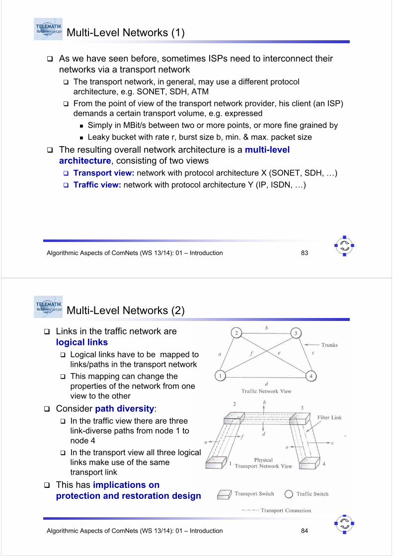
Multi-Level Networks (2)
Links in the traffic network are logical links
Logical links have to be mapped to links/paths in the transport network
This mapping can change the properties of the network from one view to the other
Consider path diversity:In the traffic view there are three link-diverse paths from node 1 to node 4
In the transport view all three logical links make use of the same transport link
This has implications on protection and restoration design
Algorithmic Aspects of ComNets (WS 13/14): 01 – Introduction 85
Chapter Summary
Data traffic is usually transported in packets that are individually forwarded through interconnected routers in the network
Routing decisions can be guided by minimizing the total “cost” of a path summing up individual link costs, and we know well established routing algorithms for this: Dijkstra’s Algorithm, Bellman-Ford Algorithm, Distance Vector Routing
Traffic can be characterized according to a stochastic process:The Poisson Process is a well established model and it shows ideal characteristics: independence, singularity, stationarity
Real Internet traffic looks different though (self similar characteristics)
Average link load should not exceed a certain threshold (e.g. 50%), otherwise long average delay occurs
Routing decisions heavily influence link utilization and should take traffic demand, link capacities, etc into account
In multi-level networks, characteristics may change between views