Embed Size (px)
Citation preview
An Investigation of Inorganic Background
Soil Constituents with a Focus on Arsenic
Species
A Thesis submitted for the degree of
Doctor of Philosophy
By
Costa J. Diomides
Victoria University
School of Molecular Sciences
September 2005

ii
Preface
I, Costa Jeremy Diomides, declare that the PhD thesis entitled “An Investigation of
Inorganic Background Soil Constituents with a Focus on Arsenic Species” is no more
than 100,000 words in length, exclusive of tables, figures, appendices, references and
footnotes. This thesis contains no material that has been submitted previously, in whole
or in part, for the award of any other academic degree or diploma. Except where
otherwise indicated, this thesis is my own work.
Signature Date

iii
Conference Presentations Relevant to the Scope of this Thesis
(1) Diomides, C., Correll, R. and Naidu, R. Assessment of aberrant levels, Fifth
National Workshop on the Assessment of Site Contamination, Environment
Protection & Heritage Council (EPHC) & National Environment Protection
Council (NEPC), Adelaide, South Australia, 13 – 15 May 2002.
(2) Diomides, C., Bigger, S. W. and Orbell, J. D. Speciation and bioavailability of
naturally elevated soil constituents (esp. arsenic), Victorian Arsenic Forum,
Environment Protection Authority – Victoria (EPAV), Melbourne, Victoria, 27
November, 2002.
Publications Relevant to the Scope of this Thesis
(1) Diomides, C., Correll, R. and Naidu, R. Assessment of aberrant levels,
Proceedings of the Fifth National Workshop on the Assessment of Site
Contamination, Environment Protection & Heritage Council (EPHC) & National
Environment Protection Council (NEPC), Adelaide, South Australia, pp 225-233.
iv
Abstract
A database was developed for the storage and convenient analysis of inorganic
background soil constituent data within specific geological groups in Victoria,
Australia. A statistical analysis of the data revealed the relative abundances of metals
and, in particular, arsenic within soils of various geological units. These units included
the Quaternary Aeolian (Qpw) (highest concentration of zinc, lowest concentration of
chromium) the Quaternary Fluvial (Qrc) (highest chromium and nickel, equal highest
copper, lowest lead and equal lowest arsenic); the Quaternary Newer Volcanics (Qvn)
(equal lowest arsenic concentration); Silurian Anderson Creek Formation (Sla) (highest
arsenic); Silurian Dargile Formation (Sud) (highest lead, equal highest copper); Tertiary
Brighton Group (Tpb) (lowest nickel) and Older Volcanics (Tvo) (lowest copper and
zinc). The identification of arsenic as a significant background constituent prompted a
formal study of this element with respect to the nature of its sorption onto different
kinds of soils, its bioavailability and speciation.
Arsenic soil sorption analyses were conducted in the laboratory on clay loam, light clay,
sand and silt loam soils. These experiments demonstrated that the sorption of arsenic
was dependent on soil type and time of soil exposure to the arsenic solution. The
bioavailability of arsenic from soil was also investigated using a relative bioavailability
test method referred to as the “geophagy gut simulation” extraction method. The
adaptation of this method to these investigations showed it to be a viable, fast and
simple technique. The experimental results indicated that the relative bioavailability of
sorbed total arsenic was dependent on soil type. Given that the toxicity of arsenic is
dependent on its speciation, techniques were also evaluated to assess arsenic speciation
in soil extracts. To this end, the utility of electrospray mass spectrometry (ESI-MS) for
the qualitative and quantitative assessment of arsenic and phosphorus speciation in
solution was explored. Although this technique yielded interesting qualitative outcomes
it was deemed not to be suitable for quantification. From the qualitative data, various
postulates were formulated for the interaction between different species that were
subsequently tested by quantum chemical calculations. A technique, based on extraction
into chloroform, for quantifying the amount of AsIII in a sample was adapted to these
investigations and was found to be highly accurate and discriminating, albeit time
consuming. All phosphorus and arsenic species found to coexist in the ESI-MS

v
experiments were modelled using high-level density functional theory (DFT). From
these calculations, the relative energies of the species could be determined as well as
reaction energies for their inter-conversion. This allowed hypotheses to be proposed for
the distribution of such species in solution and how they might be taken up into clay
structure. The DFT calculations also yielded geometrical information on a wide range of
species as well as their electrostatic potential energy maps.

vi
Acknowledgements
Sincere thanks are extended to Associate Prof. Stephen W. Bigger, principle supervisor,
and Prof. John D. Orbell, co-supervisor, for their expert supervision and guidance. The
following people are also thanked for assistance in this project:
Ms Jean Meaklim, external co-supervisor (EPAV)
Mr Vince Murone (Analytical Consulting Services)
Mr Stephen Geytenbeek (Victoria University)
Associate Prof. Neil Barnett (Victoria University)
Dr Saman Buddhadasa (NMI)
Dr Mala Santhakumar (NMI)
Mr Paul Adorno (NMI)
Mr Stavros Tzardis (NMI)
Dr Nunzio Limongiello (NMI)
Mr Leo Demel (NMI)
Mr Sebastian Barone (NMI)
All the staff at NMI for their assistance
Dr Frank Antolasic (RMIT)
Lastly, a big thankyou to my parents, sister and brother-in-law for their continued
support and encouragement.

vii
Abbreviations and Terms
AAS Atomic absorption spectrometry
AASHTO American Association of State Highway and Transportation
Officials
AB Activated Bauxsol
AFS Atomic fluorescence spectrometry
AMG Australian map grid
ANZECC Australian and New Zealand Environmental and Conservation
Council
AsIII Trivalent arsenic species
AsV Pentavalent arsenic species
AsAdj Adjusted arsenic sample concentration
AsAve Average total arsenic concentration
AsB Arsenobetain
AsBioavailability Arsenic bioavailability
AsNon-bioavailability Arsenic non-bioavailability
AsBlk Arsenic blank sample concentration
AsC Arsenocholine
ASTM American Society of Testing and materials
AsSt. Dev. Standard deviation of arsenic concentration
AsTot Total arsenic
AsTot (sorb) Total arsenic sorbed
C∞ Maximum sorption concentration
CE Capillary electrophoresis
CEC cation exchange capacity
DFT Density functional theory
DGT Diffusive gradients in thin films
DMA Dimethylarsinic acid
DTPA Diethylenetriaminepentaacetate acid
E° Standard electrode potential
EC Electrical conductivity
EDTA Ethylenediaminetetraacetic acid
EPAV Environment Protection Authority Victoria
viii
ESI-MS Electrospray Mass Spectrometry
EXAFS Extended X-ray Absorption Fine Structure
FAA Federal Aviation Administration
FAAS Flame atomic absorption spectrometry
FeIII Trivalent iron species
∆G° Gibbs free energy of formation
GC Gas Chromatography
GFAAS Graphite furnace atomic absorption spectrometry
HG Hydride generation
HGAFS Hydride generation atomic fluorescence spectrometry
HOMO Highest occupied molecular orbital
HPLC High performance liquid chromatography
ICP-AES Inductively coupled plasma atomic emission spectrometry
ICP-MS Inductively coupled plasma-mass spectrometry
IQR Interquartile range
ISSS International Soil Science Society
IUPAC International Union of Pure and Applied Chemistry
IVG In vitro gastrointestinal
IVG-AB In vitro gastrointestinal - Absorption
LC Liquid chromatography
LUMO Lowest unoccupied molecular orbital
Min minutes
MIT Massachusetts Institute of Technology
MMA Monomethylarsonic acid
MS Mass Spectrometry
m/z Mass to Charge Ratios
MW Molecular weight
NATA National Association of Testing Authorities
NEPM National Environment Protection Measure
NHMRC National Health and Medical Research Council
NMI National Measurement Institute
NZVI Nanoscale zero-valent iron
PBET Physiologically-based extraction test
pzc Point of zero surface charge
ix
Q1 First quartile
Q3 Third quartile
Qpw Quaternary Aeolian
Qrc Quaternary Fluvial
Qvn Quaternary Newer Volcanics
rpm Revolutions per minute
S1 Clay loam
S2 Light clay
S3 Sand
S4 Silt loam
SBET Simple bioaccessibility extraction test
SEP Sequential extraction procedure
SFC Supercritical fluid chromatography
SHIME Simulator of human intestinal microbial ecosystems
Sla Silurian Anderson Creek Formation
Sud Silurian Dargile Formation
TEA Triethylamine
THF Tetrahydrofuran
TMAO Trimethylarsine oxide
TOC Total organic carbon
Tpb Tertiary Brighton Group
Tvo Older Volcanics
USCS Unified Soil Classification Scheme
USDA United States Department of Agriculture
USEPA United States Environment Protection Agency
UV Ultraviolet
XAFS X-ray absorption fluorescence spectrometry
XANES X-ray absorption near edge structure
x
Table of Contents
Preface ..................................................................................................................................................... ii
Conference Presentations Relevant to the Scope of this Thesis .......................................................... iii
Publications Relevant to the Scope of this Thesis................................................................................ iii
Abstract................................................................................................................................................... iv
Acknowledgements................................................................................................................................ vi
Abbreviations and Terms...................................................................................................................... vii
1.0 Introduction................................................................................................. 1
1.1 General Overview .....................................................................................................1
1.2 Aim of Study ..............................................................................................................5
2.0 Literature Review ....................................................................................... 6
2.1 Inorganic Background Soil Data..........................................................................6
2.1.1 Overseas Data ................................................................................................6
2.1.2 Australian Data ..............................................................................................7
2.1.3 Implications of Inorganic Background Soil Data .........................................9
2.2 Factors Affecting Arsenic Sorption....................................................................11
2.2.1 Soil Particle Size and Soil Classification Systems.......................................11
2.2.1.1 Soil Classification Systems ................................................................11
2.2.1.2 Particle Size of the Soil......................................................................13
2.2.2 Time of Contact with Soil .............................................................................15
2.2.3 Temperature...................................................................................................16
2.2.4 Rate of Agitation ...........................................................................................16
2.2.5 The Effect of pH............................................................................................17
2.2.6 Sorption Materials .........................................................................................18
xi
2.3 Bioavailability of Arsenic in Soil.........................................................................20
2.4 Speciation of Arsenic in Soil................................................................................25
2.4.1 General Background Information Relating to Speciation
Analyses........................................................................................................25
2.4.1.1 Separation Methods used in Arsenic Speciation Analyses ............35
2.4.1.2 Detection Methods Used in Arsenic Speciation Analyses .............36
2.4.2 Methods Utilised for the Speciation of Arsenic in Soils .............................38
3.0 Materials and Methods ............................................................................ 43
3.1 Inorganic Background Soil Database..............................................................43
3.1.1 Development of Database...........................................................................43
3.1.2 Statistical Analysis of Data.........................................................................45
3.2 Arsenic Sorption .................................................................................................47
3.2.1 Effect of Soil Type on the Sorption of Arsenic .........................................47
3.2.2 Temporal Studies of the Sorption of Arsenic.............................................50
3.3 Bioavailability using Geophagy Method .........................................................51
3.4 Speciation Investigations ...................................................................................52
3.4.1 Electrospray Mass Spectrometry of Phosphorus and Arsenic
Species........................................................................................................53
3.4.2 Computer Modelling of ESI-MS Identified Phosphorus and
Arsenic Species ..........................................................................................53
3.4.3 Selective Organic Phase Extraction of AsIII from Soil ..............................54
3.4.3.1 Method for the Standardisation of Arsenite Sample .....................55
3.4.3.2 Method for Arsenite Sorbed onto Soil at Different pH
Values.................................................................................................55
xii
4.0 Results and Discussion ............................................................................. 58
4.1 Inorganic Background Soil Data........................................................................58
4.1.1 Arsenic ...........................................................................................................58
4.1.2 Chromium......................................................................................................60
4.1.3 Copper............................................................................................................60
4.1.4 Lead................................................................................................................61
4.1.5 Nickel .............................................................................................................62
4.1.6 Zinc ................................................................................................................64
4.2 Arsenic Sorption ...................................................................................................65
4.2.1 The Effect of Soil Type on As2O3 Sorption .................................................67
4.2.1.1 Preliminary Study on the Effect of Soil Type on As2O3
Sorption............................................................................................67
4.2.1.2 Further Analysis on the Effect of Soil Type on As2O3
Sorption............................................................................................72
4.2.2 Time Dependency of As2O3 Sorption on Soil..............................................74
4.3 Bioavailability of Arsenic.....................................................................................78
4.4 Speciation Investigations .....................................................................................82
4.4.1 Electrospray Mass Spectrometry ..................................................................82
4.4.1.1 Phosphate Speciation.........................................................................82
4.4.1.2 Arsenic Speciation .............................................................................84
4.4.2 Computer Modelling of Phosphate, Arsenate and Arsenite ........................88
4.4.2.1 Energies of Species and Reaction Energies......................................88
4.4.2.2 Geometries .........................................................................................91
4.4.2.3 Electrostatic potential energy calculations ......................................95
4.4.3 Extraction of Arsenite from Soil.................................................................106
4.4.3.1 Standardisation of Arsenite Sample................................................106
xiii
4.4.3.2 Arsenite Sorbed onto Soil at Different pH Values.........................108
5.0 Conclusions & Future Directions ......................................................... 116
5.1 Conclusions..........................................................................................................116
5.2 Future Directions................................................................................................121
6.0 References ............................................................................................... 122
Appendix A .............................................................................................. 162
Appendix B............................................................................................... 164
Appendix C .............................................................................................. 172
List of Tables
2.1 Inorganic background soil data from overseas literature 7
2.2 Inorganic background soil data from Australian literature 9
2.3 Ranges of particle size for several soil classification systems 14
2.4 Methods used to determine the bioavailability of arsenic in soils 26
3.1 Spiked levels of As2O3 used in S1, S2, S3 and S4 for total arsenic
extraction 49
3.2 Spiked levels of As2O3 used in S1, S2, S3 and S4 for bioavailable
arsenic extraction 52
4.1 Soil type characterisation 66
4.2 Effect of soil type on As2O3 sorption 68
4.3 Bioavailability results 80
4.4 Table of estimated partition coefficients 81
4.5 Phosphorus and arsenic species identified in the ESI-MS spectra
together with their relative abundance 84
4.6 Water/hydronium clusters identified in the ESI-MS spectra 86
4.7 Geometries and further information for phosphorus and arsenic
species 96
4.8 Purity of Arsenite sample 108
4.9 Amount of AsIII sorbed onto soil at different pH values 112
xiv
List of Figures
2.1 Log world average constituent concentration versus Log constituent
concentration of various countries 8
2.2 Log of the NEPM background constituent concentration versus log of
constituent concentration in various Australian capital cities 9
4.1 Summary statistics for arsenic in various geological units of
Melbourne, Australia 59
4.2 Summary statistics for chromium in various geological units of
Melbourne, Australia 61
4.3 Summary statistics for copper in various geological units of
Melbourne, Australia 62
4.4 Summary statistics for lead in various geological units of Melbourne,
Australia 63
4.5 Summary statistics for nickel in various geological units of
Melbourne, Australia 64
4.6 Summary statistics for zinc in various geological units of Melbourne,
Australia 65
4.7 Recoverable AsTot in: (a) blank and (b) soil type S1 versus the spiked
As2O3 concentration 69
4.8 Recoverable AsTot in: (a) blank and (b) soil type S2 versus the spiked
As2O3 concentration 70
4.9 Recoverable AsTot in: (a) blank and (b) soil type S3 versus the spiked
As2O3 concentration 71
4.10 Recoverable AsTot in: (a) blank and (b) soil type S4 versus the spiked
As2O3 concentration 71
4.11 Average As2O3 sorbed in soil type S1, S2, S3 and S4 at pH 2.3 and
20.3oC 73
4.12 Plot of the sorbed As2O3 versus time showing: (a) the rapid first-step
sorption process and (b) the slower second-step sorption process 74
4.13 Plot of the As2O3 sorbed in the second-step sorption process versus
time 75
4.14 A plot of ln (C∞ - Ct) for the second-step sorption process versus time 76
4.15 A plot of % AsBioavailability versus the spiked As2O3 concentration 81
xv
4.16 The ESI-MS difference spectrum obtained between anhydrous di-
sodium hydrogen orthophosphate (Na2HPO4) in water and the
background THF/water 83
4.17 The ESI-MS spectrum of anhydrous di-sodium hydrogen
orthophosphate (Na2HPO4) in water showing the water/hydronium
ion clusters that form in electrospray positive mode 85
4.18 The ESI-MS difference spectrum obtained between di-sodium
hydrogen arsenate heptahydrate (Na2HAsO4.7H2O) in water and the
background THF/water 87
4.19 The ESI-MS difference spectrum obtained between sodium arsenite
(NaAsO2) in water (pH 7.5) and the background THF/water 89
4.20 Relative computed EHOMO values 104
4.21 Relative computed ELUOMO values 104
4.22 A plot of % AsIII extracted from S2 versus pH: (a) AsIII as NaAsO2
species, (b) AsV as Na2HAsO4 species and (c) 50% v/v mixture of
AsIII and AsV stock solutions 113
4.23 A plot of % AsV extracted from S2 versus pH: (a) AsIII as NaAsO2
species, (b) AsV as Na2HAsO4 species and (c) 50% v/v mixture of
AsIII and AsV stock solutions 113
List of Charts
4.1 Electrostatic potential energy structures for PO3¯, HPO42¯ and H2PO4¯
species 99
4.2 Electrostatic potential energy structures for AsO3¯, HAsO42¯ and
H2AsO4¯ species 100
4.3 H2PO4¯ and H2AsO4¯ conformers 101
4.4 Electrostatic potential energy structures for AsO2¯, pyramidal
H2AsO3¯ and tetrahedral H2AsO3¯ species 102
4.5 Electrostatic potential energy structures for cis and trans H2AsO3¯
species 103

1
1.0 Introduction
1.1 General Overview
It is commonly know that inorganic constituents (i.e. metals/metalloids) occur naturally
in soils, usually at very low concentrations. These constituent concentrations are often
referred to as “natural background concentrations”. A suitable definition for the term
“background concentration” can be described as the concentration of a substance
consistently present in the environment that has not been influenced by localised human
activities [1]. Bedrock formed from natural geological processes undergoes weathering
and ultimately releases inorganic constituents into the soil [2-3]. Metals such as
chromium, manganese, nickel and vanadium comprise the list of some of the chemical
constituents that are referred to in inorganic background soil data [4]. However, many
other metals/metalloids can also be found in naturally occurring soil which can include:
arsenic, barium, copper, mercury, lead and zinc. The Australian and New Zealand
Guidelines for the Assessment and Management of Contaminated Sites [5] define
“background” levels as the ambient levels of substances or chemicals typically found in
the vicinity of a local area, but away from a specific activity or site. In many regards,
the two definitions of background concentration are comparable, however, the first has
more regard to natural substances that form by natural processes whereas the second
does not distinguish between human activities and natural processes. Nonetheless, both
definitions are relevant since, in many cases, it is extremely difficult to determine
whether or not natural processes alone influence background soil quality.
In some cases inorganic background soil constituents can occur, outside of mineralised
areas, at elevated levels that can be above nationally developed guidelines. In cases
where elevated inorganic background constituents are present, an understanding of the
levels that are present and the effect the constituents have on the surrounding
environment, including human health, is vital. Inorganic background soil constituents
are of interest for several reasons: (i) they can be used to characterise soil; (ii) they are
part of the nutritional food chain from soil to plants to animals (including man); and,
(iii) they are essential to the assessment of anthropogenically contaminated soil [6] in
order to compare contaminated soil levels to that of background soil constituent levels.
2
In more recent time, arsenic has become an inorganic background soil constituent of
particular interest. Arsenic has been shown to be a commonly occurring toxic metalloid
that is present in various natural ecosystems, including the terrestrial soil environment
[7]. The main source of arsenic in soil is its geological parent material with the most
elevated arsenic concentrations occurring in magmatic sulfides and iron ores. Some of
these ores include arsenic pyrites or mispickel, realgar and orpiment [7]. It has been
shown [8] that in well-oxidized and alkaline soils, Ca3(AsO4)2 is the most stable arsenic
mineral, followed by Mn3(AsO4)2. The order of increasing mineral stability is
Cd3(AsO4)2 < Pb3(AsO4)2 < Cu3(AsO4)2 < AlAsO4 < FeAsO4 < Zn3(AsO4)2 <
Ni(AsO4)2. In reduced and acidic soils, trivalent arsenic oxides and arsenic sulfides are
most stable. It has been reported that arsenic sorbed by iron, aluminium and calcium,
has a positive correlation with clay particles, in spite of the difference in texture and
organic matter content, and total nitrogen [9]. Arsenic bound to aluminium has been
shown to be more common than arsenic bound to calcium in soil samples [10].
Moreover, arsenic bound to iron in soils is the most common, however, in volcanic ash
arsenic was found to be bound to aluminium to a greater extent [11].
The main factors that affect the sorption of different forms of arsenic in soil are the type
(i.e. iron, aluminium, magnesium) and amounts of sorbing components in the soil, the
pH, the redox potential [7], the cation exchange capacity [12-13] and the clay particle
size [14]. It has been shown that soluble arsenic in soil increases with a decrease in pH
and redox potential and that the water-soluble fraction of arsenic is highest in soils that
have the lowest clay content [15]. The importance of determining the sorption qualities
of soils is two fold: (i) it provides information relating to soil-arsenic chemistry; and,
(ii) the information gained from arsenic sorption studies can be applied to the treatment
of arsenic in “real-world” environmental situations.
A notable chemical property of arsenic is its ability to form two different oxidation
states in the natural environment, namely, the pentavalent (AsV) and trivalent (AsIII)
states [16]. Both of these oxidation states are subject to chemically and
microbiologically mediated oxidation, reduction and methylation [17-19]. It has been
shown that the presence of FeIII in soils oxidizes AsIII into AsV, however, the rate of this
reaction is relatively slow [20]. Manganese dioxide or birnessite has also been shown to
be a good oxidant of AsIII species [20]. The reduction of AsV can also take place in
3
certain environments, typically in anoxic environments, in soils that contain sulfides or
in soils that contain certain microbial species [21]. Typically, AsIII is present in anoxic
conditions, while AsV is the dominant form of arsenic in oxic soils. Trivalent arsenic
may occur as uncharged As(OH)3 in acidic soils and as an anion, AsO33¯, in alkaline
soils [22]. On the other hand, AsV is present as an anion, H2AsO4¯ or HAsO42¯, in the
natural pH range of soils (pH = 4-8) [23]. The presence of arsenic as an anionic species
causes it to be quite mobile in soils when it occurs in a soluble form.
The toxicity, biological availability and transport mechanisms associated with arsenic
are highly dependent on its physicochemical form [24]. Inorganic arsenic species are
known to be more toxic than organic arsenic species [24]. With regards to inorganic
species, AsIII (arsenious acid) is more toxic, more soluble and more mobile than AsV
(arsenic acid) [25-27] whereas the organic species are generally less toxic as a result of
methylation. It has been reported that monomethylarsonic acid (MMA) is more toxic
than dimethylarsinic acid (DMA) [28]. In soils, arsenic is known to exist primarily in
inorganic forms, but MMA and DMA have also been found in some soil extracts [29-
34].
A means of determining the toxicity and biological availability of arsenic to humans is
of particular interest in order to assess the potential health implications associated with
the ingestion of arsenic, especially by children. In most cases this can only be achieved
by performing bioavailability experiments. There are a number of definitions that can
be found in the literature for the word “bioavailability”. These definitions vary
according to the field of study and reflect the importance of the chemical and biological
processes in a particular scientific discipline [35]. A general definition that is
commonly used defines bioavailability as “the degree to which a substance in a
potential source is free for uptake (movement into or onto an organism)” [36-37]. An
environmental definition states: “bioavailability is a physicochemically driven
desorption process” [38]. A suitable definition of “oral bioavailability” is “the fraction
of an administered dose that reaches the central (blood) compartment from the
gastrointestinal tract” [39]. Bioavailability defined in this manner is commonly referred
to as the “absolute bioavailability” and is equal to the oral absorption fraction [39]. In
contrast to the “absolute bioavailability” the “relative bioavailability” refers to
comparative bioavailabilities of different forms of a substance or of different exposure
4
media containing the substance (e.g. the bioavailability of a metal from soil relative to
its bioavailability from water) [39]. A distinction should also be made between the term
“bioavailability” and the term “bioaccessibility”. The latter refers to the fraction that is
soluble in the gastrointestinal environment and is available for absorption [16,39].
Bioavailability experiments can be conducted in two ways involving either in vivo
experiments or in vitro experiments. The former involves using test animals to
determine how much arsenic is sorbed by the animal’s gastrointestinal tract. From these
experiments an estimation of the bioavailability of arsenic can be calculated for the
human situation. In the case of in vitro experiments, simple extraction tests have been
used for several years to assess the degree of metals/metalloids dissolution in a
simulated human gastrointestinal tract environment [16,40-41]. Historically, relative
bioavailability estimates for metal/metalloid constituents in soil have been based on in
vivo studies in laboratory animals [39]. However, given the costs and time constraints
associated with such studies, it is clear that a more efficient alternative is desirable. The
most promising option involves the development and validation of in vitro extraction
tests that are predictive of oral metals/metalloids bioavailability from soil. Such tests
would provide a rapid and inexpensive method for developing more accurate exposure
estimates for use in human health risk assessments [39].
The bioavailability of metal/metalloid constituents is of great importance in determining
the toxicological effects of various constituents on human health as discussed above.
However, an indication of these toxicological effects can also be ascertained by
determining the chemical species of the constituents present [42]. In the past, natural
and anthropogenic soil constituents were measured based on the total content of a
specific element present in an analysed soil sample. However, the necessity to advance
our knowledge of the mobility of chemicals in soils and the physiological activity of the
inorganic elements makes necessary not only the determination of the total amount of
these elements, but also the exact determination of the concentration of their different
chemical forms [43-44]. It has been shown through biochemical and toxicological
investigations that the chemical form of a specific element, or the oxidation state in
which that element exists, is crucial in relation to its effect on living organisms [45]. To
gain information on the activity of specific elements, it is necessary to establish not only
the total content of the element but also to gain an indication of its individual chemical
5
and physical forms [45]. This approach is described as “speciation analysis”, i.e. the
quantitative estimation of the content of the different species present under those
conditions. According to the official International Union of Pure and Applied
Chemistry definition [46], speciation analysis is “the process leading to the
identification and determination of different chemical and physical forms of an element
existing in a sample”.
1.2 Aim of Study
The objective of the current study is to contribute to the knowledge of inorganic
background soil constituent levels, particularly in soils of Melbourne, Australia, by
developing a background soil constituent database. The purpose of the database is to
provide site-specific data for this region that will allow comparisons to be made against
data from known or suspected contaminated sites. Using the database the significance
of arsenic as a background soil constituent will be probed with a view to investigating
the nature of its sorption onto different kinds of soils, its bioavailability and its
speciation.
In particular, this study aims to: (i) identify the main factors that affect the sorption of
arsenic onto soil particles of four different soil types consisting of a clay loam, light
clay, sand and silt loam; (ii) estimate the proportion of total arsenic that is potentially
made available (i.e. bioavailable) to the human body from each of the soil types using a
simple in vitro procedure; (iii) investigate both qualitatively and quantitatively, the
speciation of arsenic in environmental samples; (iv) assess the applicability and the
potential use of ESI-MS to identify and characterise phosphorus (as a benchmark) and
arsenic species that originate from aqueous solutions of dissolved salts; (v) explore a
method for the quantification of arsenite in soil that involves a chloroform extraction
technique that is first used to quantify the purity of an arsenite sample utilized in
experimental work and then used to determine the amount of AsIII sorbed onto soil at
different pH values; and, (vi) assess the use of high-level density functional calculations
to provide supporting evidence for the reaction mechanisms proposed for both
phosphorus and arsenic species.
6
2.0 Literature Review
2.1 Inorganic Background Soil Data
In this section inorganic background soil data have been reviewed and compiled from
the literature. The data obtained from this review have been discussed in the following
three sections. Section 2.1.1 includes a discussion on inorganic background soil data
found in overseas literature whereas Section 2.1.2 reviews information pertaining to
Australian inorganic background soil data. The implications of inorganic background
soil data are discussed in Section 2.1.3.
2.1.1 Overseas Data
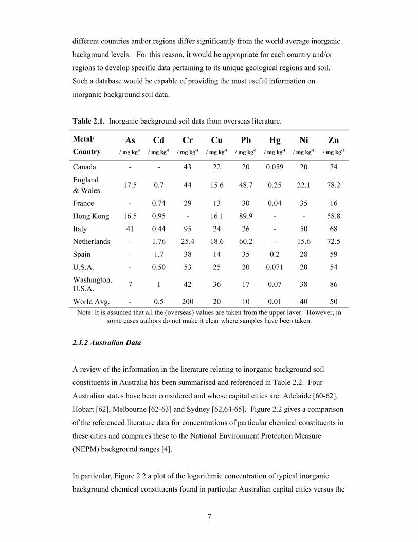
A summary of information in the literature relating to inorganic background soil
constituents in various countries and/or regions around the world is presented in Table
2.1. The countries and/or regions that have been included are: Canada [6], England &
Wales [47-52], France [53], Hong Kong [54], Italy [55], Netherlands [56], Spain [56-
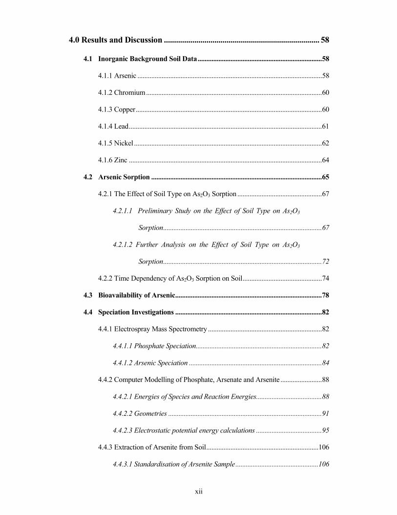
57] and U.S.A. [1,58]. Figure 2.1 is a plot of the data for concentrations of particular
chemical constituents in various countries and/or regions around the world that
compares these to world average inorganic background values [59].
Figure 2.1 is a plot of the logarithmic concentration of literature values for some typical
inorganic background chemical constituents at various international locations versus the
logarithmic concentration of the world average inorganic background values. Clearly,
the points that lie near the line of unit gradient are ones where the overseas literature
values are in close agreement with the world average inorganic background values.
Whereas, points that lie some distance from the line indicate cases where there is a
significant difference between the values. It can be seen in Figure 2.1 that for each of
the particular selected countries and/or regions the background level of chromium is
below the world average background value. However, the levels of mercury, lead, and
to a certain extent, zinc, in each of these countries and/or regions are above the
respective world average background values. Furthermore, cadmium, copper and nickel
have concentrations that are quite close to world background values. This analysis
clearly shows that the inorganic background values reported in the literature for
7
different countries and/or regions differ significantly from the world average inorganic
background levels. For this reason, it would be appropriate for each country and/or
regions to develop specific data pertaining to its unique geological regions and soil.
Such a database would be capable of providing the most useful information on
inorganic background soil data.
Table 2.1. Inorganic background soil data from overseas literature.
Metal/
Country As
/ mg kg-1
Cd / mg kg-1
Cr / mg kg-1
Cu / mg kg-1
Pb / mg kg-1
Hg / mg kg-1
Ni / mg kg-1
Zn / mg kg-1
Canada - - 43 22 20 0.059 20 74
England & Wales
17.5 0.7 44 15.6 48.7 0.25 22.1 78.2
France - 0.74 29 13 30 0.04 35 16
Hong Kong 16.5 0.95 - 16.1 89.9 - - 58.8
Italy 41 0.44 95 24 26 - 50 68
Netherlands - 1.76 25.4 18.6 60.2 - 15.6 72.5
Spain - 1.7 38 14 35 0.2 28 59
U.S.A. - 0.50 53 25 20 0.071 20 54
Washington, U.S.A. 7 1 42 36 17 0.07 38 86
World Avg. - 0.5 200 20 10 0.01 40 50 Note: It is assumed that all the (overseas) values are taken from the upper layer. However, in
some cases authors do not make it clear where samples have been taken.
2.1.2 Australian Data
A review of the information in the literature relating to inorganic background soil
constituents in Australia has been summarised and referenced in Table 2.2. Four
Australian states have been considered and whose capital cities are: Adelaide [60-62],
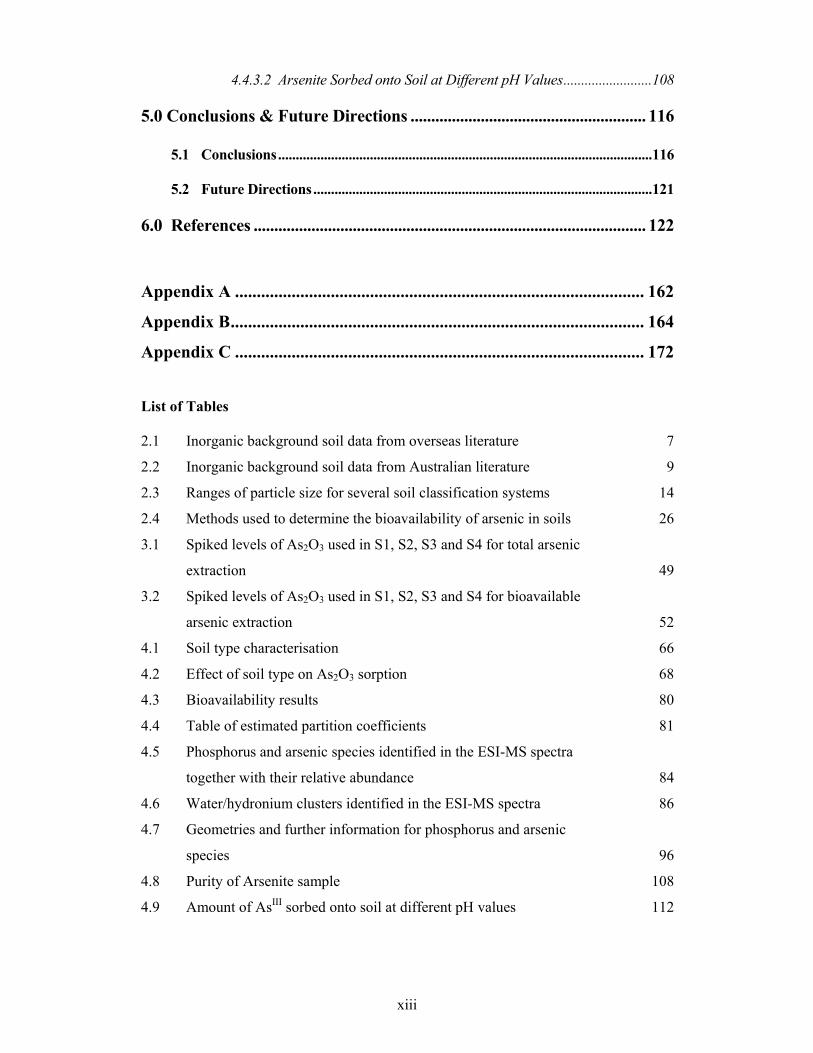
Hobart [62], Melbourne [62-63] and Sydney [62,64-65]. Figure 2.2 gives a comparison
of the referenced literature data for concentrations of particular chemical constituents in
these cities and compares these to the National Environment Protection Measure
(NEPM) background ranges [4].
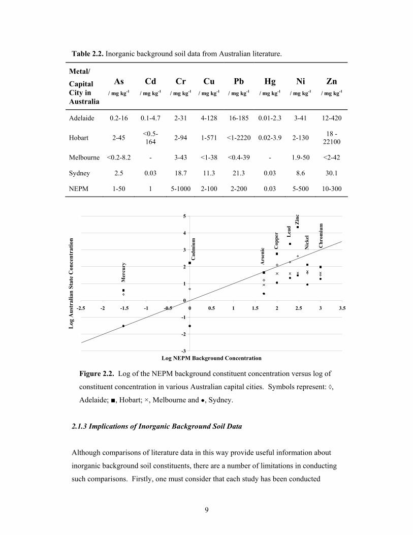
In particular, Figure 2.2 a plot of the logarithmic concentration of typical inorganic
background chemical constituents found in particular Australian capital cities versus the

8
-3
-2
-1
0
1
2
3
4
5
-2.5 -2 -1.5 -1 -0.5 0 0.5 1 1.5 2 2.5 3 3.5
Log Concentration World Average
Log
Con
cent
ratio
n V
ario
us C
ount
ries
Mer
cury
Cad
miu
m
Lea
d
Cop
per
Nic
kel
Zin
c
Chr
omiu
m
Figure 2.1. Log world average constituent concentration versus Log constituent
concentration of various countries. Symbols represent: ♦, England & Wales; ■,
France; ∆, Italy; x, Spain and +, U.S.A.
logarithmic concentration of the corresponding NEPM background values. In Figure
2.2, it can be seen that arsenic, nickel and chromium in the Australian capital cities
studied are below the NEPM background values. However, mercury, cadmium, copper
and zinc in both Hobart and Adelaide have background concentrations above the NEPM
values. Additionally, in Hobart, the background concentration of lead is also above the
corresponding NEMP value. Clearly, if the Australian background values reported in
the literature are assumed to be correct, then the data in Figure 2.2 show that each of the
capital cities studied has significantly different inorganic background constituent levels
compared to NEPM background values. General national inorganic background values
can provide useful information to an extent, however, they do not give a good indication
of typical inorganic background concentrations in a particular region, local area or
specific site [65-67]. In some groups of soil, it is supposed that soils within a given
series would have a similar chemical composition [67]. Bini et al. [55] have indicated
that the grouping of soil samples derived from the same parent material indicates that
the nature of the rock is the most important soil-forming factor. Thus, a database that
has its data categorised by parent material (i.e. geological regions) would be a most
useful resource.
9
Table 2.2. Inorganic background soil data from Australian literature.
Metal/
Capital City in Australia
As
/ mg kg-1
Cd
/ mg kg-1
Cr
/ mg kg-1
Cu
/ mg kg-1
Pb
/ mg kg-1
Hg
/ mg kg-1
Ni
/ mg kg-1
Zn
/ mg kg-1
Adelaide 0.2-16 0.1-4.7 2-31 4-128 16-185 0.01-2.3 3-41 12-420
Hobart 2-45 <0.5-164 2-94 1-571 <1-2220 0.02-3.9 2-130 18 -
22100
Melbourne <0.2-8.2 - 3-43 <1-38 <0.4-39 - 1.9-50 <2-42
Sydney 2.5 0.03 18.7 11.3 21.3 0.03 8.6 30.1
NEPM 1-50 1 5-1000 2-100 2-200 0.03 5-500 10-300
-3
-2
-1
0
1
2
3
4
5
-2.5 -2 -1.5 -1 -0.5 0 0.5 1 1.5 2 2.5 3 3.5
Log NEPM Background Concentration
Log
Aus
tral
ian
Stat
e C
once
ntra
tion
Mer
cury
Cad
miu
m
Ars
enic C
oppe
r Lea
dZ
inc
Nic
kel
Chr
omiu
m
Figure 2.2. Log of the NEPM background constituent concentration versus log of
constituent concentration in various Australian capital cities. Symbols represent: ◊,
Adelaide; ■, Hobart; ×, Melbourne and ●, Sydney.
2.1.3 Implications of Inorganic Background Soil Data
Although comparisons of literature data in this way provide useful information about
inorganic background soil constituents, there are a number of limitations in conducting
such comparisons. Firstly, one must consider that each study has been conducted

10
independently and issues associated with sampling strategies may not be standardised.
Such issues include whether single samples are used or multiple samples are
bulked/composited together, varying sampling depths, differing soil sampling intensities
and sampling location strategies which vary randomly or systematically (e.g. targeted
within a certain type of geological group) [62,67]. Very few literature studies present
inorganic background soil data based on targeted samples located within geological
regions. It also appears that targeting samples in this manner will produce extremely
useful information on inorganic soil constituents since the soil is, to an extent, related to
the parent geology [52,68-69]. It is evident that studies using a random sampling
strategy, that are not targeted within geological groups, provide information that does
not represent properly the actual background inorganic soil constituent results since
different soil groups could be mistakenly grouped together.
In a similar manner, data obtained using different analytical techniques may also be
compared inappropriately. There is no universal method of determining the total
concentration of a particular element in soil. Although there are many accepted
standard analytical methods, it is important to note that method efficiencies, sensitivity
and detection limits change with each method and will continue to change over time
[69]. In most cases it is clear that such comparisons should be avoided, however, in
some cases study constraints do not allow the ideal comparisons to be made. In cases
where different analytical techniques have been used care should be taken when
comparing the data and it should be made clear to the reader that the comparison has
this limitation.
An additional limitation with many inorganic background soil constituent studies is that
they present data for chemical constituents as a total concentration and this provides
limited information about chemical species present and the bioavailability of those
species [62]. This can be problematic because one oxidation state of a metal can be
extremely toxic, whereas the metal in a different oxidation state may be non-toxic. For
example, chromium (VI) is very toxic compared to chromium (III), which is relatively
harmless in low concentrations [70]. In cases where the total chromium concentration
is reported it does not reveal whether chromium (VI) or chromium (III) is present. This,
in turn, means that the background soil data does not give enough detail to establish the
presence of toxic or non-toxic chemical constituents. This is the case with many other
11
metal/metalloid species. For example, arsenite is considered more toxic than arsenate
[31,71] and methyl mercury is also considered to be more toxic than other inorganic
species [72]. To a large extent, it is believed [62] that naturally elevated chemical
constituents exist naturally as species that are relatively non-toxic, however, there has
been very little work done to validate this belief. It is clear that inorganic background
soil constituent data need to be scrutinised in terms of the individual chemical species
present and not just as the total concentration of chemical constituents.
2.2 Factors Affecting Arsenic Sorption
Many factors play a role in the amount of metal/metalloid concentrations that are able to
sorb onto various soil particles. In the following review, the factors controlling the
sorption of arsenic species are considered with the intent of determining which factors
are most significant. Some of the factors considered include the effect of soil particle
size, contact time, temperature, rate of agitation, pH and sorption material.
2.2.1 Soil Particle Size and Soil Classification Systems
Before the effect of soil particle size can be discussed with respect to arsenic sorption,
definitions of particle size need to be considered with respect to the various soil type
classification systems. A review of common soil classification systems is presented in
Section 2.2.1.1 that defines soil particles size for a number of soil classification systems.
This is followed in Section 2.2.1.2 by a review of information relating the effect of soil
particle size to the sorption of arsenic.
2.2.1.1 Soil Classification Systems
Many soil classification systems have been developed and used for specific purposes.
However, because different professions are interested in different soil properties, a
single descriptive soil classification system does not exist [69]. A simple method of soil
classification is based on textural properties that classify soils by particle size
distributions, taking into account the percentage sand, silt and clay content. Common
textural classification systems have been developed by the United States Department of
Agriculture (USDA) [73] and the Unified Soil Classification Scheme (USCS) [74-75].
12
These classification systems are generally used by engineers, geologists and
agriculturalists.
Other textural soil classification systems have also been developed that use different
particle size ranges. The American Association of State Highway and Transportation
Officials (AASHTO) [76] and the Federal Aviation Administration (FAA) [77] have
developed soil classification systems specifically used for road and runway
construction. A number of other soil classification systems have also been developed:
the American Society of Testing and materials (ASTM) [78], International Soil Science
Society (ISSS) [69] and Massachusetts Institute of Technology (MIT) [79].
Most of the soil classification systems discussed above have been developed in America
based on American soil properties. These systems have been extensively used in
Australia, however, they do not necessarily provide the most appropriate soil
classification for Australian soils. For this reason, the soil classification system used in
the current study has been based on an Australian system called the Northcote bolus
manipulation [80] that is an agronomical soil classification system. The Northcote
bolus manipulation method used in this study defines soil particles less than 0.002 mm
in diameter as “clays”, particles between 0.002 and 0.02 mm in diameter as “silts” and
particles ranging between 0.02 and 2 mm in diameter as “sand” with an arbitrary
separation of “coarse” and “fine” sand at 0.2 mm in particle diameter [80]. The
definitions for clay, silt and sand are similar, but not identical, to other soil classification
techniques. For example, the USDA defines soil particles in the following manner: (i)
total clay, <0.002 mm; (ii) total silt, range between 0.002 to 0.05 mm; and, (iii) total
sand, ranging between 0.05 to 2.00 mm. The USDA method has various other sub-
classifications within these groups for coarse, medium and fine silts and sands [73].
The other soil classification systems: AASHTO, FAA and USCS, all have similar
particle size definitions to the Northcote bolus manipulation system but, nonetheless,
are still slightly different [69]. It is evident that the classification of soils in
environmental studies is problematic because a standard technique has not been
adopted. Various professional groups like engineers, geologists and agriculturalists
require specific classification techniques for their own purpose. However, due to the
overlap between environmental disciplines, one soil classification system may not
13
service the requirements of all involved and would require a system that best suits the
given situation.
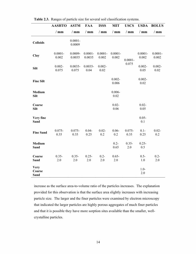
A table defining the soil particle sizes for each of the soil classification systems
discussed above has been presented in Table 2.3. On close examination of the
information summarized in Table 2.3 it can be seen that the soil particle sizes for most
of the classification systems are similar. Interestingly, a comparison between the ISSS
and the BOLUS system indicate that the two systems are almost identical in soil particle
size distribution, suggesting that perhaps the BOLUS system is based on the
internationally developed ISSS system.
2.2.1.2 Particle Size of the Soil
A review of information relating to the effect of particle size on the sorption of arsenic
species was conducted. It has been shown by Singh et al. [81-82] that with the decrease
in sorbent-particle size the extent of AsV removal increases for both hematite and
feldspar. This has been explained on the basis of surface area per unit mass available
for the sorption of AsV, where the surface area will be greater for smaller particles. The
extent and rate of sorption both increase with a decrease in particle size and can be
attributed to the following: (i) the increased surface area of the hematite/feldspar due to
a smaller particle size will attract more AsV species on its surface as the number of
active sites increases; (ii) when the diffusive path-length into the interior of the
hematite/feldspar particles is reduced, the AsV species require less energy to jump from
one active site to another active site and thus the rate-of-jump and finally the sorption
increases; and, (iii) small particles move faster in solution than large ones and hence
there will be a greater shearing effect due to collections and intraparticle effects on their
surface [81-82].
In contrast to the findings of Singh et al. [81-82], Genc-Fuhrman et al. [83] have
indicated that the larger particle size of activated seawater-neutralized red mud or
activated Bauxsol (AB) is able to sorb/remove more AsV than AB with smaller particle
size. The increased removal efficiency for the larger particles was reported as surprising
because the efficiency of surface sorption processes would normally be expected to
14
Table 2.3. Ranges of particle size for several soil classification systems.
AASHTO ASTM FAA ISSS MIT USCS USDA BOLUS
/ mm / mm / mm / mm / mm / mm / mm / mm
Colloids 0.0001-0.0009
Clay 0.0001- 0.002
0.0009-0.0035
0.0001-0.0035
0.0001-0.002
0.0001-0.002
0.0001- 0.002
0.0001-0.002
Silt 0.002- 0.075
0.0035-0.075
0.0035-0.04
0.002-0.02
0.0001-0.075
0.002- 0.05
0.002- 0.02
Fine Silt 0.002-0.006 0.002-
0.02
Medium Silt 0.006-
0.02
Coarse Silt 0.02-
0.06 0.02- 0.05
Very fine Sand 0.05-
0.1
Fine Sand 0.075- 0.35
0.075-0.35
0.04- 0.25
0.02- 0.2
0.06- 0.2
0.075-0.35
0.1- 0.25
0.02- 0.2
Medium Sand 0.2-
0.65 0.35- 2.0
0.25- 0.5
Coarse Sand
0.35- 2.0
0.35- 2.0
0.25- 2.0
0.2- 2.0
0.65- 2.0 0.5-
1.0 0.2- 2.0
Very Coarse Sand
1.0- 2.0
increase as the surface area-to-volume ratio of the particles increases. The explanation
provided for this observation is that the surface area slightly increases with increasing
particle size. The larger and the finer particles were examined by electron microscopy
that indicated the larger particles are highly porous aggregates of much finer particles
and that it is possible they have more sorption sites available than the smaller, well-
crystalline particles.
15
In another interesting study [84] it has been suggested that the particle size varies with
pH which influences the concentration of AsV sorption onto goethite. At pH = 3
goethite particles present much smaller diameters, hence showing higher surface areas,
important for the effective sorption of metal ions, while at pH = 5 larger goethite
particles can be observed, decreasing the removal efficiency of this sorbent towards
AsV.
It is evident that the particle size of soil has a significant effect on the sorption of
arsenic, however, it appears that the particle size is influenced by the sorption material
that is present within a given system [81]. When comparing the particle size within the
same sorption material it would appear that the smaller particles are able to sorb arsenic
better. However, this may not be the case when comparing the arsenic sorption
qualities of different sorbing materials as shown in the activated Bauxsol example [83].
2.2.2 Time of Contact with Soil
In a number of studies, the effect of the time of contact on the sorption of various
arsenic species (commonly AsV and AsIII) has been reviewed for different soil sorption
materials. In a study performed by Genc-Fuhrman et al. [83], the time to reach
equilibrium for the sorption of AsV onto an activated seawater-neutralized red mud,
commonly referred to as an activated Bauxsol, is reported as 3 h [85]. The equilibrium
process reported for AsIII on AB was shown to remove arsenic shortly after the initial
shaking commenced and increased over time until a steady state was reached after
approximately 6 h. The results for both AsV and AsIII indicate the first-order nature of
the adsorption process and suggest that the process depends on both the solution
concentration and the number of available adsorption sites.
In an alternative study [81], the sorption of AsV by hematite and feldspar as a function
of the time of contact for different initial concentrations at optimum pH and temperature
was investigated. It was found, in that study, that sorption is rapid during the initial
stages and then approaches equilibrium after 35 min for hematite and 60 min for
feldspar at each concentration. The results indicate the independent nature of the
equilibrium period for the solute concentration. Similar observations were noted at
different temperatures and pH. It was also noted that the adsorption of AsV increases
16
more for hematite than it does for feldspar when the solute concentration increases.
There is an approximate ten-fold increase at optimum pH and temperature.
Similar to the studies reviewed to this point, Zeng [86] also investigated the effect of the
time of contact on arsenic sorption using several sorbents, including a silica-containing
iron (III) oxide sorbent. The results of the arsenic sorption tests show that the contact
time over the tested range of 1–7 days has a trivial influence on the arsenic sorption.
From the reviewed studies it can be concluded that the time of contact varies greatly
depending on the solute concentration and sorbent material. It appears the composition
of the sorbent material has a significant effect on the time required for arsenic
absorption. For example, in sorbent materials that contain more iron (hydr)oxides the
time of contact required for arsenic sorption is far less than in sorbent materials that
contain little or no iron (hydr)oxides. The effects of other sorbent materials, including
iron (hydr)oxides, are reviewed in more detail in Section 2.2.6.
2.2.3 Temperature
The results of certain studies [81,87] suggest that the sorption of AsV increases (i.e.
removal decreases) for both hematite and feldspar upon increasing the temperature from
20 to 40°C indicating the process to be exothermic. This may be attributed to the
relative increase in the tendency of the solute to escape from the solid phase to the bulk
phase with the rise in the temperature of the solution. This is in agreement with work
conducted by Genc-Fuhrman et al. [83] who suggest that the increase in sorption with
temperature in activated Bauxsol is due to the increased rate of diffusion of sorbate
molecules into the pores of the material.
2.2.4 Rate of Agitation
The rate of agitation has a significant effect on the sorption of arsenic species as
reported by Singh et al. [81]. In that study, the extent of AsV sorption was found to
increase with an increase in the rate of agitation up to 125 rpm. Beyond an agitation
rate of 125 rpm the extent of AsV sorption stays almost constant. This was found to be
in good agreement with the findings of earlier workers [88-89]. It is evident that the
17
rate of adsorption is controlled by the degree of agitation to a certain extent as the
increasing agitation reduces the boundary-layer resistance to mass transfer and increases
the mobility of the system [88]. It seems that for agitation rates below 125 rpm, film
transport is important, whereas at speeds of 125 rpm and above, the intraparticle
diffusion becomes important [89].
2.2.5 The Effect of pH
In a study [83] using an activated Bauxsol it was suggested that the sorption process is
pH dependent, favouring AsV sorption at pH values below 7.0 and AsIII sorption at a pH
of 8.5. It was suggested that arsenate sorption on AB is a ligand-based adsorption. It
was also suggested that the pH dependence of arsenic sorption onto AB can be further
understood by investigating the point of zero surface charge (pHpzc). The pHpzc is
where the surface charge switches from negative (at higher pH) through zero to positive
(at lower pH values). When the pH is below the pHpzc the solid surface is positively
charged and favours the adsorption of AsV anions (e.g. H2AsO4¯, HAsO42¯), but when
the pH is above the pHpzc the surface of the solid is negatively charged and anion
adsorption must compete with Coulombic repulsion. The composition of Bauxsol has a
complex mixture of different minerals, with each mineral having different pHpzc values
[90]. These minerals can have different surface charges at a given pH that gives AB the
capacity to remove arsenic over a wide pH range. The fact that AB sorbs AsV more
efficiently at pH < 7.0 and decreases rapidly for pH > 7.0 may reflect the importance of
hematite and maghemite in the sorption process [91]. Similar findings have been
reported by others [92] who have shown that the adsorption of AsV on metal oxides and
oxyhydroxides increases at lower pH values and gradually decreases at higher pH
values. It has also been shown that the maximum sorption occurs for AsIII at pH values
between 7.0 and 8.5 for red mud and amorphous oxides [91,93].
In another study [94] it has been suggested that AsV typically exhibits pH dependent
adsorption onto Fe oxides [95]. Similar findings have also been suggested in other
studies [81,96] indicating that the removal of AsV by hematite and feldspar is pH
dependent. In these studies the amount of AsV adsorbed increases with rising pH and
reaches a maximum concentration at pH = 4.2 and pH = 6.2 for hematite and feldspar
respectively. Among the different species of AsV, the H2AsO4¯ species is predominant
18
within the pH range 2.0 to 7.0 and above this range the HAsO42¯ species is dominant up
to pH 11.0 [87]. The adsorption of arsenate is favoured electrostatically up to the
pHpzc of the adsorbents but beyond this point specific adsorption plays an important
role [96]. The decrease in the extent of adsorption below pH = 4.2 in the case of
hematite and below pH = 6.2 in the case of feldspar may be attributed to the dissolution
of the adsorbents and a consequent decrease in the number of adsorption sites [97]. The
maximum removal around pH = 4.2 and pH = 6.2 with different adsorbents used, is
attributed to surface complexation [97].
In solution, it has been suggested [28] that the arsenic species present depend on the pH
and the redox activity of the system and a Pourbaix diagram (See Appendix A) has been
constructed [28] for various AsIII and AsV species that exist at different pH values. The
Pourbaix diagram indicates that under oxidizing conditions AsV species are present at
the following pH values: (i) at pH < 2 the H3AsO4 species is present; (ii) between pH =
2 and pH = 7 H2AsO4¯ is present; (iii) between pH = 7 and pH = 11.5 HAsO42¯ is
present; and, (iv) at pH > 11.5 the AsO43¯ species is present. Under reducing conditions
AsIII species are present at the following pH values: (i) pH < 7.5 H3AsO3 is present; (ii)
between pH = 7.5 and pH = 12 the H2AsO3¯ species is present; and, (iii) at pH > 12 the
HAsO32¯ species is present. From that study it is clear that pH and redox activity play
an important role in determining the species of arsenic that are present, and this, in turn,
affects the species of arsenic that are able to sorb onto a sorption material such as soil.
2.2.6 Sorption Materials
In a study completed by Yang et al. [94] it was determined that the Fe oxide content of
the soil is the major factor governing the initial adsorption of AsV by the soil. It was
shown that the percentage of AsV adsorbed increases sharply as the Fe oxide content
increases, indicating the important role of Fe oxide in providing binding sites for AsV.
Of the eight soils in that study with less than 5 g kg-1 of Fe oxides, none adsorbed more
than 60% of the added AsV. When the Fe oxide concentration was above 5 g kg-1, 27 of
28 soils adsorbed greater than 80% of the dissolved arsenic. Zhang and Stanforth [98]
also reported similar results and indicated that iron oxides and oxyhydroxides
(ferric(hydr)oxide), which are present in soils, sediments, and aquatic environments,
have a strong affinity for arsenic species [99-101]. Goethite (α-FeOOH) has been
19
widely used as a representative iron oxide in adsorption studies because it is widespread
in nature, can be synthesized readily in the laboratory, and has a well characterized
structure [102]. Adsorption of arsenate on hydrous iron oxides has been shown to
initially occur rapidly followed by a slow sorption stage thereafter [95,103-105]. Other
studies [106-107] have suggested that iron and aluminium oxides adsorb anionic arsenic
species well in acidic soils, whereas calcium oxides in alkaline soils adsorb anionic
arsenic species to a lesser extent.
In an alternative investigation, two types of reference materials, a hydrous ferric oxide
(FeOOH) and a SiO2 gel, were tested for adsorption of AsV and AsIII following a batch
adsorption procedure [86]. The experiments showed that arsenic removal by FeOOH
was 100% for AsV (at pH = 6.5) and 99.5% for AsIII (at pH = 7.3), whereas arsenic
removal by SiO2 was only 6.8% for AsV and 0% for AsIII (both at pH = 6.9). The high
capacity of FeOOH for absorbing each of the AsV and AsIII species has also been
reported by other researchers [95,108-109]. By contrast, SiO2 gel can adsorb very little
AsV and AsIII. It was however, suggested that the addition of SiO2 can influence arsenic
adsorption in two ways: (i) the co-precipitated silica has no arsenic adsorption qualities,
but may cover some active sites on FeOOH. When a high silica content is present, the
coverage of SiO2 on the FeOOH surface is likely to become significant, leading to a
lowering of arsenic adsorption; and, (ii) dissolved silica species may compete with
arsenic for adsorption sites on FeOOH since the silica has a relatively higher solubility
compared to FeOOH. It has been shown that the dissolved silica species can
significantly inhibit the adsorption of arsenic and some other trace metals in aqueous
solutions [110-111].
It has been suggested in a number of other investigations that a wide range of possible
adsorbents are responsible for arsenic removal including goethite and gibbsite [112-
113], ferrihydrite and hydrous ferric oxides [103,114-115], hematite [116], activated red
mud [91], and Bauxsol and activated Bauxsol [85,117]. Many of these sorbents may be
used for arsenic removal in water systems, however, arsenic removal in large-scale
water treatment plants usually involves coagulation with Fe or Al salts [83,118-119].
Processes based on adsorption and coprecipitation methods are significant because they
can be used in small scale treatment plants and household systems, are easy to operate,
may provide largely sludge-free operation, and may have a regeneration capability [120].
20
In research reported by Kanel et al. [121], a synthetically prepared nanoscale zero-
valent iron (NZVI) was tested for the removal of AsIII. The adsorption kinetics of the
system were rapid, occurring in only minutes. Batch experiments were performed to
determine the feasibility of NZVI as an adsorbent for AsIII treatment in groundwater as
affected by initial AsIII concentration and pH (pH = 3-12). The investigation confirmed
that NZVI and AsIII form inner-sphere surface complexes. The effects of competing
anions showed HCO3¯, H4SiO4 and H2PO42¯ are potential interferences in the AsIII
adsorption reactions. The results suggest that NZVI is suitable for both in-situ and ex-
situ groundwater treatment due to its high reactivity.
The literature indicates that there are many different materials that show good physical
and chemical properties for the sorption of arsenic species. A family of substances that
has been extensively mentioned in the literature as most suitable sorption materials for
arsenic are the iron (hydr)oxides. Many of these iron (hydr)oxides are used in their
mineral (natural) forms, like goethite, gibbsite, hematite and maghemite, whereas others
may be modified or synthetically prepared to maximise the arsenic sorption qualities. It
is clear that the material substrate plays a vital role in the sorption of arsenic and also
has an influence over the particle size distribution. The pH of the system also plays a
significant role in determining the amount of arsenic that is sorbed and, more
importantly, the actual arsenic species that is present is of most importance in
determining the toxicity of this metalloid and its availability to living organisms.
2.3 Bioavailability of Arsenic in Soil
Many studies have been performed to investigate bioavailability with a view to
determining the availability of particular constituents to living organisms in order to
determine their associated toxicities. However, the review presented here focuses on
the methods used to determine the bioavailability of arsenic in soil.
In the past, the oral toxicity values obtained for arsenic have been derived from
epidemiological studies of arsenic in water [16,122]. In these studies it has been
suggested that the absorption of soluble arsenic ingested by humans is close to 100%
and that absorption occurs in the gastrointestinal tract [16,40,123]. However, in

21
contrast to arsenic in water, arsenic in soil generally exists as mineral forms or as soil-
arsenic complexes that will be incompletely solubilised during transit through the
gastrointestinal tract. Consequently, arsenic in soil will be absorbed less than arsenic in
water given that arsenic must be dissolved in order for it to be absorbed [16,124].
Experimental work using arsenic-contaminated soil [40] has confirmed that post-
ingestion absorption of arsenic from most solid-phase compounds is likely to be
substantially lower. In studies that assume 100% absorption of arsenic, the
bioavailability is significantly over-estimated [39-40,94,125].
It has been suggested that the bioavailability of arsenic in soil can be divided into two
kinetic steps; (i) dissolution of arsenic in gastrointestinal fluids; and, (ii) absorption
across the gastrointestinal epithelium into the bloodstream [126]. The biological and
chemical processes that take place in the gastrointestinal tract are extremely complex
which means they are difficult to simulate in the laboratory [126]. For this reason many
arsenic bioavailability studies are performed using controlled dosing studies involving
animals, in order to estimate arsenic bioavailability in humans. Studies of this nature
are referred to as in vivo bioavailability studies.
In a study [127] where the absolute arsenic bioavailability was determined in a
contaminated residential soil and house dust, the bioavailabilities were determined to be
between 20% and 28% (expressed relative to soluble arsenic in urine) when ingested by
Cynomolgus monkeys [124]. In that study [127] it was suggested that in the event of
ingestion of soils containing smelter waste, arsenic bioavailability will be constrained
by encapsulation in insoluble matrices (e.g., enargite in quartz), formation of insoluble
precipitates (e.g., iron hydroxide and silicate precipitating on arsenic phosphate grains),
and formation of iron-arsenic oxide and arsenic phosphate cements that reduce the
arsenic bearing surface area available for dissolution [94,124,127-128]. These
geochemical and physical limitations together with kinetic limitations associated with
dissolution of these phases during the short transit time through the gastrointestinal tract
help explain the reduced bioavailability noted in other investigations using these
materials [124,127].
Using a rat model [42], in an alternative study, the absolute bioavailability of arsenical
pesticide-contaminated soils relative to AsIII or AsV ranged from 1.02 to 9.87% and 0.26
22
to 2.98%, respectively (as determined using urinary arsenic measurements). In this
particular study it was attempted to develop a suitable leachate test as an index of
bioavailability. However, the results indicated that there is no significant correlation
between the bioavailability and leachates using neutral pH water or 1 M HCl. The
results also indicated that speciation is highly significant for the interpretation of
bioavailability and risk assessment data. The bioavailable fractions of arsenic in these
contaminated soils were shown to be low, suggesting a limited health impact to the
environment and humans.
Numerous researchers have attempted to correlate in vivo experiments with in vitro
experiments in order to develop relative bioavailability tests that are simple, convenient
and reproducible [39,42,129]. A comparison of a physiologically-based extraction test
(PBET) with in vivo studies for both rabbits and Cynomolgus monkeys was conducted
to determine how well the in vivo experiments correlate to the PBET [16]. It was
determined that the relative arsenic bioavailability in a residential soil sample was 48%
in the in vivo rabbit experiment [130] versus 57% in PBET. The relative arsenic
bioavailability in the in vivo monkey experiment was 20% [131] versus 31% in PBET.
In both cases the PBET relative arsenic bioavailability conservatively overestimates the
relative arsenic bioavailability compared to the two animal models, however, the results
of the PBET indicate good predictive ability for arsenic bioavailability from soil. In
another study [128], excellent agreement was found between the in vivo and in vitro
availability of arsenic (11% versus 12%) which suggests that the in vitro dissolution
methodology (based on a simulated gastrointestinal tract of a rabbit) replicates arsenic
dissolution in the New Zealand White rabbit gastrointestinal tract.
In a study completed by Rodriguez et al. [129] an in vitro gastrointestinal (IVG) method
based on a human model was developed to estimate the bioavailability of arsenic in
contaminated soil from mining/smelter sites. In this method, the arsenic was extracted
from the soil using simulated gastric and intestinal solutions. A variation to this method
was also made, where iron hydroxide gel was used, in a second method, referred to as
IVG-AB, to simulate the absorption of arsenic in a process analogous to that of food
absorption in the gastrointestinal tract. In this study the in vitro arsenic bioavailability
results were compared to in vivo results determined from dosing trials using immature
swine and the results ranged from 2.7 to 42.8% arsenic bioavailability. The study
23
indicated that arsenic extracted by the IVG and IVG-AB methods were not statistically
different to arsenic measured using the in vivo method. The study indicated that all IVG
methods extract similar amounts of arsenic and thereby provide reliable estimates of
bioavailable arsenic in a contaminated soil. In the same study a comparison was also
made with the PBET method. The results indicated that the PBET stomach phase does
not correlate well with the in vivo swine model, while the PBET intestinal phase does
produce a positive correlation.
The estimated arsenic bioavailability using the IVG method in soils contaminated with
arsenical pesticides was also completed by Sarkar and Datta [132]. In their study the
IVG method was slightly modified to increase its accuracy in estimating the
bioavailability of arsenic. In addition to simulating arsenic dissolution in gastric and
intestinal solutions, absorption by the intestinal membrane was mimicked using iron-
oxide coated filter paper strips inserted in nylon bags. In this method the intestinal
lining is better physically simulated using iron-oxide coated filter paper strips compared
to the iron hydroxide gel used by Rodriguez et al. [129] without adding to the total
volume of the digestive solution. The in vitro experiments were sequentially performed
in two phases, namely, the stomach phase and the absorbed-intestinal phase. Arsenic
extraction in the in vitro absorbed intestinal phase increased, thereby making it more
comparable to a potential in vivo arsenic method.
A study describing a multi-laboratory comparison and evaluation of five in vitro
digestion models was conducted [133]. The five methods compared in this study were
as follows: (i) the simple bioaccessibility extraction test (SBET method) that simulates
mobilisation of contaminants in the acid conditions of the stomach and does not employ
an intestinal compartment. The SBET method was first described by Ruby et al.
[16,41] who validated it against in vivo swine studies; (ii) the German E DIN 19738
(DIN) method is based on an in vitro digestion model. It is a static in vitro
gastrointestinal model that uses synthetic gastric and intestinal digestive juices that can
be used with or without the influence of food in the presence of milk powder; (iii) the
Netherlands in vitro digestive model, referred to as the RIVM method, is also based on
a static in vitro gastrointestinal model that allows the soil to be subjected to a number of
stages simulating the human digestive process; (iv) the “simulator of human intestinal
microbial ecosystems of infants” (SHIME) method utilises a static gastrointestinal
24
system wherein the different digestive juices are added to the same reactor; and, (v) the
TNO gastrointestinal model, referred to as the “TIM method”, is a dynamic model that
simulates the transit through the gastrointestinal tract, the gastric and intestinal pH
profiles and the secretion of digestive juice over time. The comparison of the five in
vitro bioavailability methods revealed that for arsenic bioaccessibility, the simplest,
SBET method, produces results similar to those of the more complicated TIM method.
The three soils, that were used in the study [133], indicated: (i) for soil “Flanders”
SBET bioaccessibility was 50% versus 52% for the TIM method; (ii) for soil “Oker 11”
SBET bioaccessibility was 11% versus 15 % for TIM; and, (iii) for soil “Montana
2711” SBET 59% versus 50 % for TIM. These results suggest that the bioaccessibility
of arsenic in the acidic environment of the stomach is the rate determining step in
controlling arsenic sorption as opposed to sorption across the intestinal epithelium as
reported by Ruby et al. [39].
An extremely simple relative bioavailability method has been described by certain
researchers [134-135] who have used the ‘geophagy’ (gut simulation) method to
estimate the proportion of mineral nutrients available to the human body. The method
simulates mobilisation of mineral nutrients in the acid conditions of the stomach and
does not employ an intestinal compartment. In a study undertaken by Ruby et al. [39] it
was concluded that the extent of arsenic dissolution in the acidic environment of the
stomach is predictive of relative oral bioavailability of arsenic in the animal models.
Although arsenic is sorbed through the intestinal epithelium, the results suggest that the
rate-controlling step in arsenic sorption is dissolution in the stomach rather than
sorption across the intestinal epithelium. This suggests that using a simple gastric
digestion model to estimate the relative bioavailability can provide meaningful results
that would cost significantly less in comparison to performing in vivo experiments.
Rodriguez et al. [129] also found that the simpler gastrointestinal models appear to
correlate better with in vivo studies. In that study it was concluded that no in vitro
model will exactly replicate in vivo bioavailability because the human digestive system
is too complex and dynamic to simulate in the laboratory. It was suggested that perhaps
the best way forward would involve developing an in vitro method that is based upon
human gastrophysiology that correlates well with an in vivo method. From this
correlation, mathematical relationships can be developed that will be useful in making
risk estimates.
25
A summary of the methods that can be used to determine the bioavailability of arsenic
in soils is presented in Table 2.4.
2.4 Speciation of Arsenic in Soil
A review of the literature relating to the speciation of arsenic in soil has been
performed. The first part of this review, Section 2.4.1, considers general background
information relating to speciation. This is followed by Section 2.4.2, a review of the
methods that are specifically utilised to identify the speciation of arsenic in soils.
2.4.1 General Background Information Relating to Speciation Analyses
Many studies have been completed which utilise the technique of chemical speciation
analysis to identify the chemical and physical forms of a constituent in a particular
sample. However, much of the published work on metal speciation has dealt with the
determination of metal species in natural waters, with papers on metal speciation in
solid matrices scattered in the literature [43]. This is particularly the case for arsenic
speciation in soils.
Many of the studies that appear in the literature concentrate on developing improved
methods for speciation analysis that aim to solve existing problems. One of the main
difficulties encountered in speciation analyses of soil samples is extracting the required
constituent(s) from the solid state. In most cases the nature of the analytical equipment
that must be used requires that the sample be dissolved. However, soils and sediments are
resistant to complete dissolution [28] and the dissolution of soils may alter the species that
were initially present. Using a chemical extractant is usually the most common form of
extracting the chemical constituent of interest, however, careful selection of the chemical
extractant is required. The chemical extraction reagents may themselves alter the
indigenous speciation of elements [43,136]. It should also be noted that extractants that are
less powerful leaching solutions are probably more selective for specific fractions than are
more severe reagents but the overall efficiency of extraction may be lower [43,136].
It is, therefore, important that the extraction methods are efficient and minimize the
destruction of the arsenic species present in the solid materials [137]. For example, the
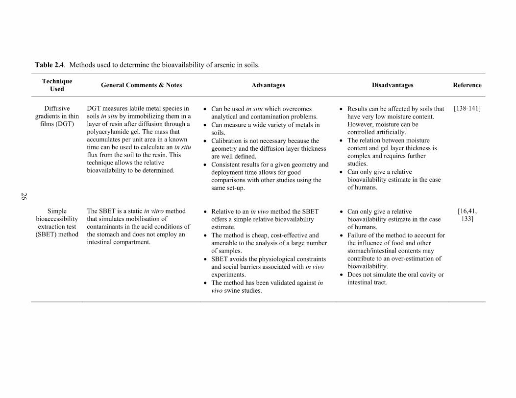
26
Table 2.4. Methods used to determine the bioavailability of arsenic in soils.
Technique Used General Comments & Notes Advantages Disadvantages Reference
Diffusive
gradients in thin films (DGT)
DGT measures labile metal species in soils in situ by immobilizing them in a layer of resin after diffusion through a polyacrylamide gel. The mass that accumulates per unit area in a known time can be used to calculate an in situ flux from the soil to the resin. This technique allows the relative bioavailability to be determined.
• Can be used in situ which overcomes
analytical and contamination problems. • Can measure a wide variety of metals in
soils. • Calibration is not necessary because the
geometry and the diffusion layer thickness are well defined.
• Consistent results for a given geometry and deployment time allows for good comparisons with other studies using the same set-up.
• Results can be affected by soils that
have very low moisture content. However, moisture can be controlled artificially.
• The relation between moisture content and gel layer thickness is complex and requires further studies.
• Can only give a relative bioavailability estimate in the case of humans.
[138-141]
Simple
bioaccessibility extraction test
(SBET) method
The SBET is a static in vitro method that simulates mobilisation of contaminants in the acid conditions of the stomach and does not employ an intestinal compartment.
• Relative to an in vivo method the SBET
offers a simple relative bioavailability estimate.
• The method is cheap, cost-effective and amenable to the analysis of a large number of samples.
• SBET avoids the physiological constraints and social barriers associated with in vivo experiments.
• The method has been validated against in vivo swine studies.
• Can only give a relative
bioavailability estimate in the case of humans.
• Failure of the method to account for the influence of food and other stomach/intestinal contents may contribute to an over-estimation of bioavailability.
• Does not simulate the oral cavity or intestinal tract.
[16,41, 133]
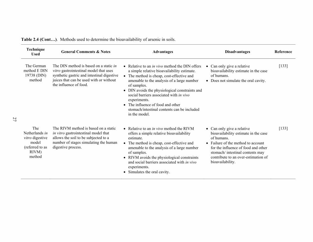
27
Table 2.4 (Cont…). Methods used to determine the bioavailability of arsenic in soils.
Technique Used General Comments & Notes Advantages Disadvantages Reference
The German
method E DIN 19738 (DIN)
method
The DIN method is based on a static in vitro gastrointestinal model that uses synthetic gastric and intestinal digestive juices that can be used with or without the influence of food.
• Relative to an in vivo method the DIN offers
a simple relative bioavailability estimate. • The method is cheap, cost-effective and
amenable to the analysis of a large number of samples.
• DIN avoids the physiological constraints and social barriers associated with in vivo experiments.
• The influence of food and other stomach/intestinal contents can be included in the model.
• Can only give a relative
bioavailability estimate in the case of humans.
• Does not simulate the oral cavity.
[133]
The
Netherlands in vitro digestive
model (referred to as
RIVM) method
The RIVM method is based on a static in vitro gastrointestinal model that allows the soil to be subjected to a number of stages simulating the human digestive process.
• Relative to an in vivo method the RIVM
offers a simple relative bioavailability estimate.
• The method is cheap, cost-effective and amenable to the analysis of a large number of samples.
• RIVM avoids the physiological constraints and social barriers associated with in vivo experiments.
• Simulates the oral cavity.
• Can only give a relative
bioavailability estimate in the case of humans.
• Failure of the method to account for the influence of food and other stomach/ intestinal contents may contribute to an over-estimation of bioavailability.
[133]
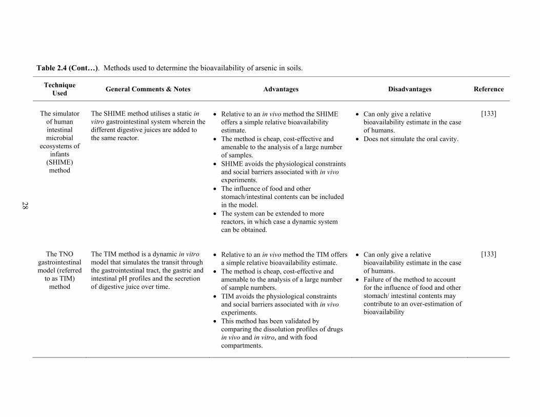
28
Table 2.4 (Cont…). Methods used to determine the bioavailability of arsenic in soils.
Technique Used General Comments & Notes Advantages Disadvantages Reference
The simulator
of human intestinal microbial
ecosystems of infants
(SHIME) method
The SHIME method utilises a static in vitro gastrointestinal system wherein the different digestive juices are added to the same reactor.
• Relative to an in vivo method the SHIME
offers a simple relative bioavailability estimate.
• The method is cheap, cost-effective and amenable to the analysis of a large number of samples.
• SHIME avoids the physiological constraints and social barriers associated with in vivo experiments.
• The influence of food and other stomach/intestinal contents can be included in the model.
• The system can be extended to more reactors, in which case a dynamic system can be obtained.
• Can only give a relative
bioavailability estimate in the case of humans.
• Does not simulate the oral cavity.
[133]
The TNO
gastrointestinal model (referred
to as TIM) method
The TIM method is a dynamic in vitro model that simulates the transit through the gastrointestinal tract, the gastric and intestinal pH profiles and the secretion of digestive juice over time.
• Relative to an in vivo method the TIM offers
a simple relative bioavailability estimate. • The method is cheap, cost-effective and
amenable to the analysis of a large number of sample numbers.
• TIM avoids the physiological constraints and social barriers associated with in vivo experiments.
• This method has been validated by comparing the dissolution profiles of drugs in vivo and in vitro, and with food compartments.
• Can only give a relative
bioavailability estimate in the case of humans.
• Failure of the method to account for the influence of food and other stomach/ intestinal contents may contribute to an over-estimation of bioavailability
[133]
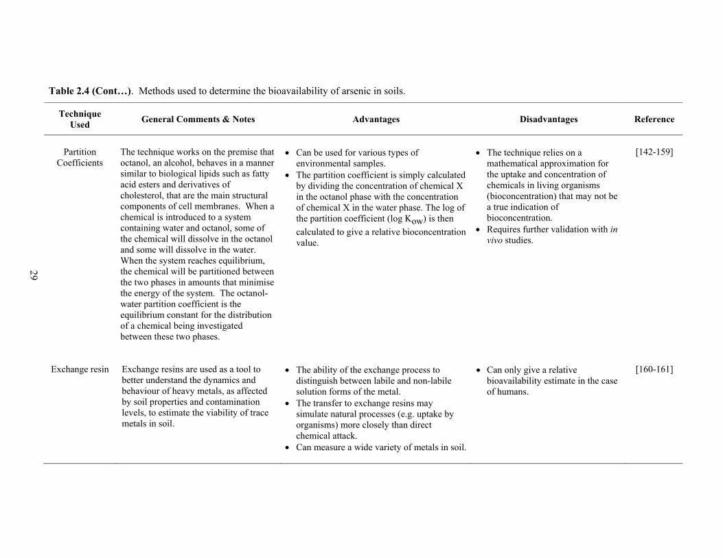
29
Table 2.4 (Cont…). Methods used to determine the bioavailability of arsenic in soils.
Technique Used General Comments & Notes Advantages Disadvantages Reference
Partition
Coefficients
The technique works on the premise that octanol, an alcohol, behaves in a manner similar to biological lipids such as fatty acid esters and derivatives of cholesterol, that are the main structural components of cell membranes. When a chemical is introduced to a system containing water and octanol, some of the chemical will dissolve in the octanol and some will dissolve in the water. When the system reaches equilibrium, the chemical will be partitioned between the two phases in amounts that minimise the energy of the system. The octanol-water partition coefficient is the equilibrium constant for the distribution of a chemical being investigated between these two phases.
• Can be used for various types of
environmental samples. • The partition coefficient is simply calculated
by dividing the concentration of chemical X in the octanol phase with the concentration of chemical X in the water phase. The log of the partition coefficient (log Kow) is then calculated to give a relative bioconcentration value.
• The technique relies on a
mathematical approximation for the uptake and concentration of chemicals in living organisms (bioconcentration) that may not be a true indication of bioconcentration.
• Requires further validation with in vivo studies.
[142-159]
Exchange resin
Exchange resins are used as a tool to better understand the dynamics and behaviour of heavy metals, as affected by soil properties and contamination levels, to estimate the viability of trace metals in soil.
• The ability of the exchange process to
distinguish between labile and non-labile solution forms of the metal.
• The transfer to exchange resins may simulate natural processes (e.g. uptake by organisms) more closely than direct chemical attack.
• Can measure a wide variety of metals in soil.
• Can only give a relative
bioavailability estimate in the case of humans.
[160-161]
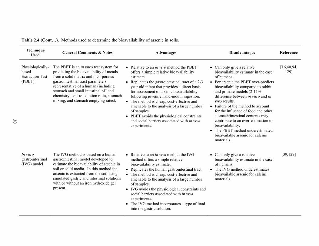
30
Table 2.4 (Cont…). Methods used to determine the bioavailability of arsenic in soils.
Technique Used General Comments & Notes Advantages Disadvantages Reference
Physiologically-based Extraction Test (PBET)
The PBET is an in vitro test system for predicting the bioavailability of metals from a solid matrix and incorporates gastrointestinal tract parameters representative of a human (including stomach and small intestinal pH and chemistry, soil-to-solution ratio, stomach mixing, and stomach emptying rates).
• Relative to an in vivo method the PBET
offers a simple relative bioavailability estimate.
• Replicates the gastrointestinal tract of a 2-3 year old infant that provides a direct basis for assessment of arsenic bioavailability following juvenile hand-mouth ingestion.
• The method is cheap, cost-effective and amenable to the analysis of a large number of samples.
• PBET avoids the physiological constraints and social barriers associated with in vivo experiments.
• Can only give a relative
bioavailability estimate in the case of humans.
• For arsenic the PBET over-predicts bioavailability compared to rabbit and primate models (2-11% difference between in vitro and in vivo results.
• Failure of the method to account for the influence of food and other stomach/intestinal contents may contribute to an over-estimation of bioavailability.
• The PBET method underestimated bioavailable arsenic for calcine materials.
[16,40,94,
129]
In vitro gastrointestinal (IVG) model
The IVG method is based on a human gastrointestinal model developed to estimate the bioavailability of arsenic in soil or solid media. In this method the arsenic is extracted from the soil using simulated gastric and intestinal solutions with or without an iron hydroxide gel present.
• Relative to an in vivo method the IVG
method offers a simple relative bioavailability estimate.
• Replicates the human gastrointestinal tract. • The method is cheap, cost-effective and
amenable to the analysis of a large number of samples.
• IVG avoids the physiological constraints and social barriers associated with in vivo experiments.
• The IVG method incorporates a type of food into the gastric solution.
• Can only give a relative
bioavailability estimate in the case of humans.
• The IVG method underestimates bioavailable arsenic for calcine materials.
[39,129]
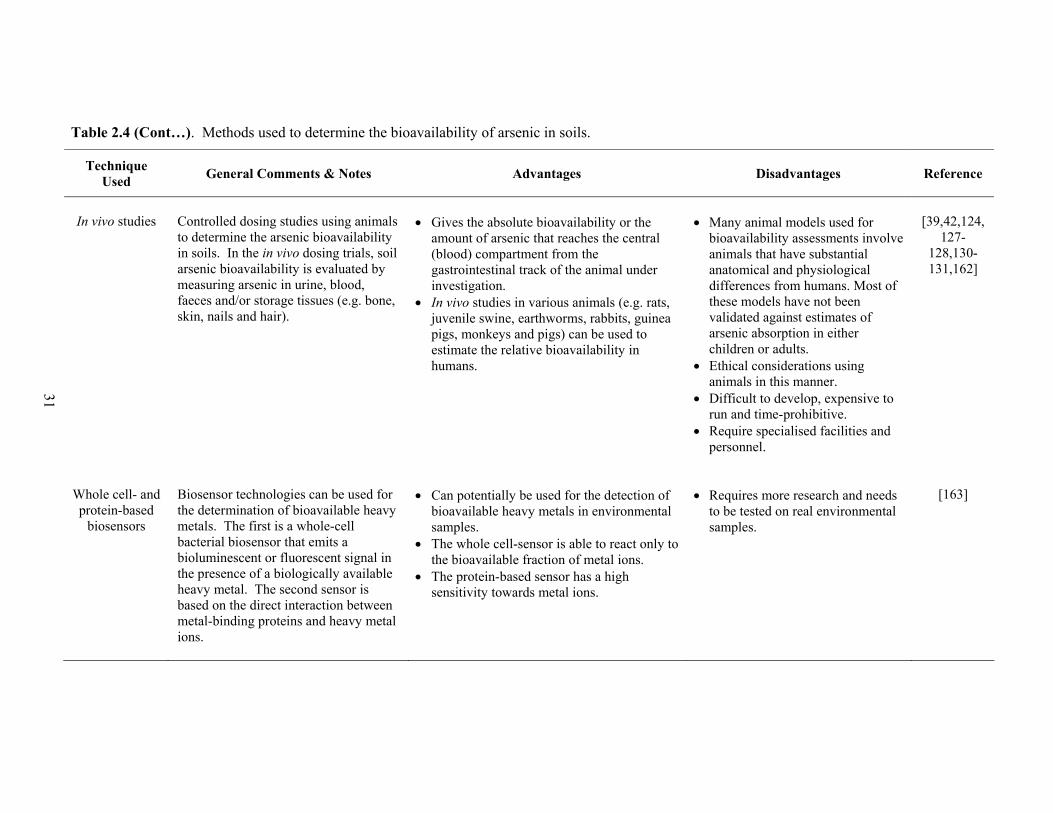
31
Table 2.4 (Cont…). Methods used to determine the bioavailability of arsenic in soils.
Technique Used General Comments & Notes Advantages Disadvantages Reference
In vivo studies
Controlled dosing studies using animals to determine the arsenic bioavailability in soils. In the in vivo dosing trials, soil arsenic bioavailability is evaluated by measuring arsenic in urine, blood, faeces and/or storage tissues (e.g. bone, skin, nails and hair).
• Gives the absolute bioavailability or the
amount of arsenic that reaches the central (blood) compartment from the gastrointestinal track of the animal under investigation.
• In vivo studies in various animals (e.g. rats, juvenile swine, earthworms, rabbits, guinea pigs, monkeys and pigs) can be used to estimate the relative bioavailability in humans.
• Many animal models used for
bioavailability assessments involve animals that have substantial anatomical and physiological differences from humans. Most of these models have not been validated against estimates of arsenic absorption in either children or adults.
• Ethical considerations using animals in this manner.
• Difficult to develop, expensive to run and time-prohibitive.
• Require specialised facilities and personnel.
[39,42,124,
127-128,130-131,162]
Whole cell- and protein-based
biosensors
Biosensor technologies can be used for the determination of bioavailable heavy metals. The first is a whole-cell bacterial biosensor that emits a bioluminescent or fluorescent signal in the presence of a biologically available heavy metal. The second sensor is based on the direct interaction between metal-binding proteins and heavy metal ions.
• Can potentially be used for the detection of
bioavailable heavy metals in environmental samples.
• The whole cell-sensor is able to react only to the bioavailable fraction of metal ions.
• The protein-based sensor has a high sensitivity towards metal ions.
• Requires more research and needs
to be tested on real environmental samples.
[163]
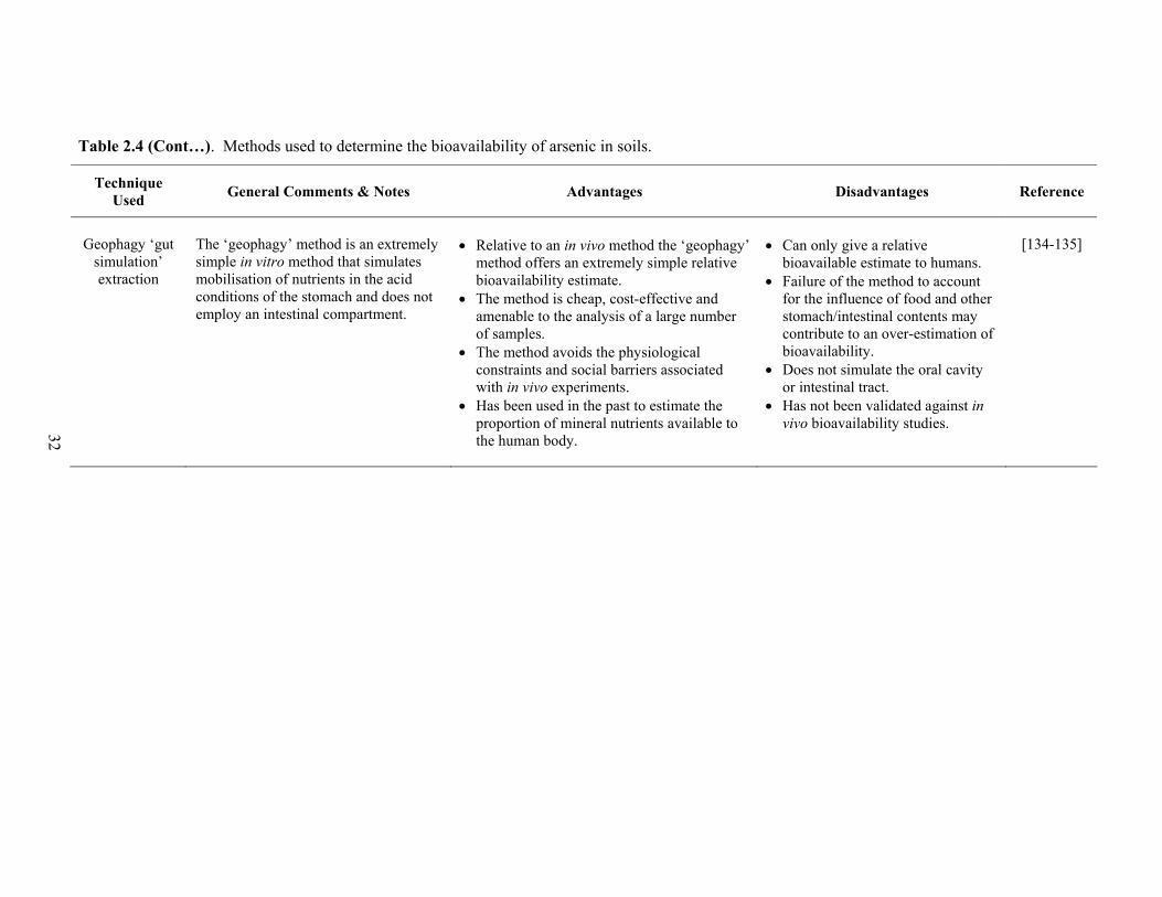
32
Table 2.4 (Cont…). Methods used to determine the bioavailability of arsenic in soils.
Technique Used General Comments & Notes Advantages Disadvantages Reference
Geophagy ‘gut
simulation’ extraction
The ‘geophagy’ method is an extremely simple in vitro method that simulates mobilisation of nutrients in the acid conditions of the stomach and does not employ an intestinal compartment.
• Relative to an in vivo method the ‘geophagy’
method offers an extremely simple relative bioavailability estimate.
• The method is cheap, cost-effective and amenable to the analysis of a large number of samples.
• The method avoids the physiological constraints and social barriers associated with in vivo experiments.
• Has been used in the past to estimate the proportion of mineral nutrients available to the human body.
• Can only give a relative
bioavailable estimate to humans. • Failure of the method to account
for the influence of food and other stomach/intestinal contents may contribute to an over-estimation of bioavailability.
• Does not simulate the oral cavity or intestinal tract.
• Has not been validated against in vivo bioavailability studies.
[134-135]

33
application of an extractant such as hydrofluoric acid could prove to be unsuitable for
soil speciation analysis because it is likely to destroy the silicate soil lattice and liberate
all of the constituent elements present in the sample [164-165]. This extraction
technique may be suitable for a total metal extraction but would probably not be specific
enough for speciation analyses.
Many researchers [43,165-177] have conducted experiments to determine appropriate
metal extractants for the determination of metals/metalloids in soil samples. The
extraction procedures have included either single leaching steps or combined sequential
extraction schemes, with the latter being more suitable for the speciation of
metals/metalloids in soils [43]. Extractants such as neutral electrolytes, e.g. CaCl2 or
MgC12, buffers of weak acids, e.g. acetic acid or oxalic acid, chelating agents, e.g.
ethylenediaminetetraacetic acid (EDTA) or diethylenetriaminepentaacetate acid
(DTPA), redox agents, e.g. NH2OH, strong acids, e.g. HC1, HNO3, HClO4 or HF, or
bases, e.g. NaOH or Na2CO3 have been considered [43] and the advantages and
disadvantages of each have been discussed. It has been suggested [43] that the ability of
various extractants to release metal ions depends on their association with particular soil
fractions. Extractants such as electrolytes, weak acids and chelating agents release
metals from coordination sites, while strong acids and other redox agents are capable of
releasing additional quantities of metals as a result of the decomposition of the solid
matrix.
The number of papers reporting extractants specifically developed for the extraction of
arsenic from soils is limited within the literature [178]. In a study conducted by Wenzel
et al. [179-180], a sequential extraction procedure (SEP) was developed for arsenic by
choosing extraction reagents commonly used for the sequential extraction of selenium
and phosphorus. The reliability of this method has been discussed by its proponents
[179]. The SEP for arsenic includes the following five extraction steps: (i) 0.05 M
(NH4)2SO4, 20°C, 4 h; (ii) 0.05 M NH4H2PO4, 20°C, 16 h; (iii) 0.2 M ammonium
oxalate buffer in the dark, pH = 3.25, 20°C, 4 h; (iv) 0.2 M ammonium oxalate buffer
and ascorbic acid, pH = 3.25, 96°C, 0.5 h; (v) HNO3/H2O2 microwave digestion.
Within the inherent limitations of chemical fractionation, these arsenic fractions appear
to be primarily associated with: (i) non-specifically sorbed; (ii) specifically-sorbed; (iii)
amorphous and poorly-crystalline hydrous oxides of Fe and Al; (iv) well-crystallized
hydrous oxides of Fe and Al; and (v) residual phases [179].

34
The results of another study [181] revealed the arsenic extraction efficiencies of 14
reagents increases in the following order: deionized water ~ 1 M NH4Cl ~ 0.5 M NH4Ac
~ 0.5 M NH4NO3 ~ 0.5 M (NH4)2SO4 < 0.5 M NH4F < 0.5 M NaHCO4 < 0.5 M
(NH4N)2CO3 < 0.05 M HCl < 0.025 M H2SO4 < 0.5 M HCl < 0.5 M Na2CO3 < 0.5 M
KH2PO4 < 0.5 M H2SO4 ~ 0.1 M NaOH. A four step sequential extraction procedure
was also developed by Polyak and Hlavay [182] for the extraction of the nine
metals/metalloids including arsenic. The four sequential extraction steps included the
following extractants: (i) CH3COOH at pH = 2.8, adjusted by HNO3 to determine the
exchangeable metals and metals bound to carbonate; (ii) NH2OH at pH = 2, adjusted by
HCl to determine the metals bound to Fe/Mn oxide; (iii) H2O2, at pH 2–3 to determine
the metals bound to organic matter and sulfides; and, (iv) HNO3 and HClO4 to
determine the acid soluble metal content.
The extraction of both arsenic and zinc from a contaminated soil was reported [183]
using various extraction methods to determine which method was most efficient. The
extraction methods were tested and validated using a reference soil sample. The three
extractive agents tested were: (i) 0.0625 M EDTA disodium salt; (ii) 0.005 M DPTA
with 0.01 M CaCl2 and 0.1 M triethylamine (TEA); and, (iii) 0.005 M DPTA in a single
extraction. It was found that 0.005 M DPTA extracts the highest quantity of arsenic and
was subsequently chosen for further assays using sonication. It was found that the
sonication time reached a plateau after 9 min and increasing the sonication frequency
increases arsenic extraction. It was concluded that in the extraction of arsenic and zinc
sonication can be used to replace extraction with mechanical shaking in order to
simplify analytical procedures when many samples need to be tested.
Once the metals have been extracted from the soil using a suitable extraction medium,
the solution can be analyzed using instrumental techniques that have sufficient
selectivity and sensitivity. The rapid analysis of samples to prevent species conversion
is also important [137]. Instrumental techniques used for speciation analyses generally
have two components: (i) a selective separation component; and, (ii) a sensitive
detection component. Often techniques are combined to achieve both selectivity and
sensitivity. The direct coupling of a separation device to various detection instruments
enables improved specificity and detection for individual arsenic species [137]. These
kinds of techniques are referred to as “hyphenated techniques”.

35
2.4.1.1 Separation Methods used in Arsenic Speciation Analyses
A number of different kinds of separation devices can be used in hyphenated techniques
for the speciation of arsenic. One of the more common separation techniques is high
performance liquid chromatography (HPLC) [184-190]. Other such separation
techniques include capillary electrophoresis (CE) [191-193], supercritical fluid
chromatography (SFC) [193] and gas chromatography (GC), the last having been
applied to arsenic speciation analysis in fewer cases.
The main forms of HPLC separation techniques used for the speciation of arsenic
include: (i) anion-exchange HPLC with either isocratic elution [194-202] or gradient
step elution [203-206]; (ii) cation-exchange HPLC with isocratic elution [196,198,201];
and (iii) reversed-phase ion-pair HPLC used in conjunction with appropriate counter
ions in the mobile phase and incorporating isocratic [207-211] or gradient elution [201].
In order to separate arsenic anions and cations in a single run, a column-switching
system involving a combination of anion-exchange and reversed-phase HPLC has also
been developed [212].
Both anion- and cation- exchange HPLC techniques have been used for arsenic
speciation analysis in the literature discussed above. Depending on the ionic
characteristics of the arsenic compounds, anion exchange is the most commonly used
technique used to analyze AsIII, AsV, MMAV and DMAV, whereas cation exchange is
used to separate arsenobetain, arsenocholine, trimethylarsine oxide and Me4As+ species.
The arsenic species separated using ion exchange HPLC are summarized in a review
paper prepared by Gong et al. [137]. In a similar manner to ion exchange HPLC, ion-
pair HPLC techniques have also been developed for the separation of arsenic species.
Tetrabutylammonium (both hydroxide and phosphate) is the common pairing cation for
separating AsIII, AsV, MMAV and DMAV. The resolutions of these arsenic species
depend on the concentration of the ion-pair reagent, the flow rate, ionic strength, and pH
of the mobile phase [213-214]. The optimum pH range for separating the four arsenic
species is between 5.0 and 7.0 [137].
The use of CE as a separation device has also been reported in a number of studies
[186,191,193]. Some of the advantages of CE include its ability to separate complex
mixtures of ionic species very quickly and efficiently and its ability to discriminate the

36
speciation pattern of redox-sensitive elements and organometallics, including arsenic
species. In addition, CE has good tolerance to complex sample mixtures, requires very
little sample, and minimal sample pre-treatment is required [186]. The limitation of CE
is its lack of compatibility with several of the more sensitive methods of detection.
However, further research on this issue may overcome this problem in the future.
2.4.1.2 Detection Methods Used in Arsenic Speciation Analyses
The separation techniques, mentioned above in Section 2.4.1.2, are often coupled to
sensitive detection devices. This section discusses the devices used in some of these
hyphenated techniques for the sensitive detection of arsenic species.
In the past, a common detection device used was flame atomic absorption spectrometry
(FAAS) [194-195,206]. However, because FAAS suffers from low sensitivity and high
background noise for arsenic determination, most recent applications of atomic
absorption spectrometry (AAS) are combined with hydride generation (HG)
[184,197,200,215-219]. HGAAS allows for extremely low detection limits. However,
not all arsenic species form hydrides, and decomposition techniques are usually
required. Graphite furnace atomic absorption spectrometry (GFAAS) has also been
used as a detection device applied to arsenic speciation. Nonetheless, a direct coupling
of HPLC to GFAAS has proven to be difficult [137,214,220]. A novel hyphenated
technique utilizes thermospray nebulization of the HPLC effluent followed by
thermochemical hydride generation in combination with AAS [221]. Electrothermal
AAS has also been used as an off-line detector of the separated arsenic species
[201,210,222].
Inductively coupled plasma atomic emission spectrometry (ICP-AES) has been
successfully coupled to HPLC for use in arsenic speciation [194,196,202,204-205,211-
212,220,223-224]. The coupling is straightforward because the usual flow rate under
which an HPLC operates is compatible with the uptake flow rate of an ICP-AES system
[137]. A number of applications have been demonstrated, primarily for samples
containing high levels of arsenic. For systems containing lower levels of arsenic,
HPLC-ICP-AES does not provide sufficient sensitivity for arsenic speciation. Several
studies incorporating HG between HPLC and ICP-AES to enhance the sensitivity [225-
228] have also been reported.
37
Inductively coupled plasma-mass spectrometry (ICP-MS) has become a favoured
detection technique in arsenic analysis [184,207-208,229-234]. It provides ultra-
sensitivity, multi-element capability and can be combined with most separation
techniques for speciation analysis. The multi-element capability allows for the
simultaneous determination of different elements in addition to arsenic [137]. ICP-MS
has also been coupled with CE detection however the method has shown mixed levels
of success [235-237]. Two major problems are the mismatch of sample volume
between CE and ICP-MS and the suction generated by nebulization. To solve these
problems, several interfaces between CE and ICP-MS have been developed. Although
some progress has been made using this technique, the matrix effect and poor sensitivity
limit CE-ICP-MS to standard solutions and simple systems.
Another hyphenated technique that has been used to detect arsenic species is hydride
generation atomic fluorescence spectrometry (HGAFS) coupled to HPLC. The
advantages of this technique are its powerful ability to selectivity separate and
sensitively detect arsenic species. Detection limits in the order of sub-microgram per
liter have been achieved for arsenic speciation [238-240]. These are comparable to
those achieved by HPLC-ICP-MS using pneumatic nebulization. The HPLC-HGAFS
techniques have been applied to the speciation of arsenic in various environmental and
biological samples [238-241].
In more recent time, electrospray ionization mass spectrometry (ESI-MS) has been
repeatedly shown to be well suited for arsenic speciation, either used alone or in
combination with HPLC [242-248]. Unlike ICP-MS, ICP-AES, AAS, and AFS, where
elemental arsenic is detected, ESI-MS can provide molecular information of arsenic
compounds for positive identification. Due to the availability of the structural
information provided by ESI-MS, a number of studies have focused on the
characterization and identification of organoarsenicals, such as arsenosugars and new
arsenic species [242,245,249-254]. Corr and Larsen [242] first demonstrated the use of
positive-ion ESI-MS for determining dimethylated arsenosugars at trace levels.
Others have coupled supercritical fluid extraction with AAS [255] and CE with ICP-
AES [256] in order to perform arsenic analyses. Other methods utilise the coupling of
ion exchange chromatography with ICP-MS [257-260]. Most of these researchers

38
discuss the benefits and drawbacks of their particular arrangement while some suggest
how further improvements can be made to existing equipment.
Overall, it can be seen that some of the HPLC-atomic spectrometry techniques
mentioned above require either costly equipment, such as ICP instrumentation, or
systems developed “in-house” that are not readily available to many laboratories. These
factors limit the use of these technologies at present. It is hoped that these technologies
will become more affordable and more accessible in the future. The appropriate use of
such technical equipment is also a limiting factor. In most cases specially trained
personnel are required to maintain and operate such equipment to prevent misuse and
misinterpretation of results.
2.4.2 Methods Utilised for the Speciation of Arsenic in Soils
One of the earliest know methods used for the speciation of arsenic in soils was reported
by Forehand et al. [261] in 1976. The method used in this work is based on a method
reported some years earlier [262] that utilized benzene as a highly selective and
sensitive extractant for AsIII (from a HCl medium) to separate arsenic from antimony
and bismuth. In the Forehand et al. [261] method the soil sample is digested in HCl and
this is followed by the reduction of AsV to AsIII using SnCl2 and KI. Benzene is used to
extract the AsIII which is then back extracted into water and analysed using AAS. The
method relies on the premise that AsIII is selectively extracted into an organic phase (i.e.
benzene) from a strongly acidic phase that can then be back extracted into water for
analysis. In the presence of excess HCl, chlorination of the arsenic will occur, resulting
in arsenic trichloride and arsenic pentachloride. It has been shown that the arsenic
trichloride is a covalent molecule while arsenic pentachloride most likely exists as ion
complexes [263]. The arsenic trichloride is extracted selectively into the organic phase
while arsenic pentachloride is excluded due its ionic properties. The arsenic trichloride
contained in the organic phase can be recovered by back extraction with water, since
arsenic is most stable in solution in its hydrolysed form [264-265].
Takamatsu et al. [29] in 1982 used almost the same method as Forehand et al. [261] to
determine arsenic species in a contaminated soil. In that study, an analytical technique
that consists of a sequential extraction using HCl, HCl/KI, benzene and H2O/H2O2
followed by anion-exchange chromatography and final determination of arsenic by

39
flameless AAS is reported. Studies have been completed by others [32,42] who have
utilized a similar speciation method to that of Forehand et al. [261] and Takamatsu et al.
[29] however in some cases the solvent benzene has been substituted with chloroform.
In 1984, Maher [266] reported a speciation method to determine the arsenic species in a
marine sediment. The method involves extracting the arsenic from the solid phase using
HCl and NaOH/NaCl solution. The extracted arsenic species are then separated by
solvent extraction and ion exchange chromatography and determined by AAS. The
sediment extract has been found to contain 45-90% inorganic arsenic (i.e. AsIII and
AsV), 4-39% monomethyl arsenic species and 4-22% as dimethyl arsenic species.
However, the method does not enable the elucidation of whether the methylated species
were due to material entering the sediments in this form (i.e. from anthropogenic inputs
or from natural marine plankton or other organic remains) or whether they were
produced by chemical reactions within the sediment [28].
In a study conducted in 1992 [267], arsenic speciation analyses were conducted on soil
samples that had been contaminated with an arsenic wood preservation material. A
portion of each soil sample was extracted with water using ultrasonic treatment for a
duration of 60 min. The establishment of the treatment was not stated in the reference.
The mixture was filtered under pressure and then injected without further purification
into a HPLC system for separation. Seven arsenic species were separated isocratically
by anion- and cation- exchange HPLC in less than 4 min. Arsenic detection was carried
out using an arsenic-specific FAAS detector with a hydrogen-argon flame that was
optimized and modified for best achievable detection limits, and was interfaced on-line
to the HPLC system. The advantage of this particular set-up is its simplicity and the
common, moderately-priced equipment of which it is comprised. The detection limits
obtained with the HPLC-FAAS system are sufficiently low for selected applications,
including arsenic speciation in contaminated soils. The arsenic speciation results
obtained using the HPLC-FAAS were compared with results obtained from the same
HPLC separation system, this time, interfaced to the more powerful ICP-MS detector.
The comparison confirmed the data obtained with the HPLC-FAAS system, but also
emphasized that the latter system can only be applied to certain practical arsenic
speciation problems.
40
In some cases the analysis of solid extraction residues by X-ray absorption fluorescence
spectrometry (XAFS) has also been used for arsenic speciation analysis [268]. The
XAFS technique has also been used to determine arsenic oxidation states, local
coordination, and the relative proportion of different arsenic species in three California
mine wastes [269]. X-ray absorption near edge structure (XANES) analysis indicated
that AsV was the dominant oxidation state in the mine samples, but mixed oxidation
states (nominally As0 and AsV) were observed in one of the three wastes [269].
In the late 1990s, a reported procedure for the extraction and separation of alkylarsenic
species from Buffalo River Sediment standard reference material was developed [230].
The sample was sonicated in methanol-hydrochloric acid-water mixture (50:10:40%
v/v) and filtered. The arsenic species in the extract were separated by anion exchange
HPLC, using phosphate (pH = 6.0) and citrate (pH = 6.0) buffers as eluents, and
detected by direct aspiration into an ICP-MS. Helgesen and Larsen [21] also used
HPLC coupled with on-line ICP-MS to separate and selectively detect arsenic species in
food and environmental samples (including soil samples) at their naturally occurring
concentrations [270]. However, in this study, the soil samples were extracted using a
calcium nitrate solution in which the samples were soaked for 1 h with gentle
mechanical shaking at room temperature. The supernatant was separated from the soil
solids by centrifugation prior to injection into the HPLC-ICP-MS system for arsenic
speciation determination. The anion-exchange HPLC column was eluted isocratically
using an ammonium carbonate solution containing 97% v/v water and 3% v/v methanol
(at pH = 10.3) as the mobile phase. The eluate from the HPLC system was
continuously introduced into the ICP-MS instrument that enabled the determination of
AsIII, AsV, MMA and DMA.
In a more recent study completed by Bissen and Frimmel [24] the speciation of AsIII,
AsV, MMA and DMA were reported by extracting the arsenic species from soil
samples. The samples were sequentially extracted with 0.3 M ammonium oxalate (pH =
3, adjusted with 0.3 M oxalic acid), milli-Q water (pH = 5.8), 0.3 M sodium bicarbonate
(pH = 8) and 0.3 M sodium carbonate (pH = 11). After the extraction procedure, the
samples were filtered, diluted if necessary, and analyzed immediately by HPLC-ICP-
MS. The separation of arsenic species was performed by an anionic exchange HPLC
system containing a microporous resin bed consisting of ethylvinylbenzene crosslinked
with 55% divinylbenzene having alkanol quaternary ammonium groups on latex

41
particles. The HPLC system was coupled with an ICP-MS detector (using NaOH as the
mobile phase).
In 2001, a study [271] was conducted to determine the AsIII, AsV, MMA and DMA
concentrations in three reference materials, namely river sediment, agricultural soil,
sewage sludge, that had been certified for their total arsenic content. The analytical
method included an ion exchange liquid chromatography separating device coupled on-
line to a HGAFS detector. Prior to analysis, the arsenic species were extracted from the
soils using orthophosphoric acid that was chosen as a “soft” extractant able to dissolve
arsenic species without modifying them [272]. The efficiency of this extraction
procedure was studied in detail and was found to be more dependent upon the nature of
the material analysed than on the acid concentration. Recoveries of 90–100% of total
arsenic were obtained for the sediment and sludge reference materials whereas a 62%
recovery was obtained for the soil reference materials. It was found that the method
provides very low detection limits and has a high sensitivity for both the analysis of
arsenic-poor samples and the dilution of arsenic-rich extracts. It was concluded that the
proposed method has very good potential as a routine speciation analysis procedure for
arsenic speciation studies in environmental solids. In a slightly earlier study, Thomas et
al. [273] also used a phosphoric acid extraction method to speciate arsenic in soil and
sediment samples. The extracts were then analysed using HPLC coupled to ICP-MS.
Another method reported for the speciation of arsenic in soils is based on the extraction
of arsenic using phosphoric acid and ascorbic acid [274]. The arsenic extract is then
analysed using a multiple hyphenated technique that includes the coupling of liquid
chromatography (LC), ultraviolet (UV) irradiation, HG and ICP-MS. This speciation
method has been applied to several contaminated soils. It showed that AsV is the main
species in the soils and that in some samples AsIII and methylated species could also be
detected. The same study also compared results obtained using the LC-UV-HG-ICP-
MS speciation technique with those obtained using a varied speciation technique, LC-
UV-HG-AFS. The findings revealed that LC-UV-HG-AFS is adequate for arsenic
speciation in soils to detect both inorganic and organic species. However, the findings
also indicated that the ICP-MS coupled detection system is much more sensitive.
In 2003, an alternative study [275] was reported that utilized HPLC coupled to ICP-MS.
In this study the efficiency of consecutive extractions using several individual
42
extractants or solvent mixtures was evaluated. The extractants included: water,
methanol/water and phosphoric acid for arsenic species extracted from rice, fish,
chicken tissue and soil samples. The analysis revealed the presence of AsIII, AsV, MMA
and DMA in the soil samples and that 1 M phosphoric acid was found to be the most
efficient extractant. It was also revealed that MMA and DMA are stable in 1 M
phosphoric acid extracts from soils whereas AsIII gradually oxidizes to AsV.
Overall, it is evident that most speciation analyses are limited by the soil extraction
procedure. The soil extractants used are not necessarily capable of extracting all the
arsenic specifically from the soil and, even more importantly, there can be no certainty
that the arsenic species remain in their indigenous form (i.e. extractants most likely alter
the natural species in the soil upon extraction). More research is required for many of
these extractants to validate their use in arsenic speciation analyses.
It would also be of great value to adopt a (validated) standard arsenic extraction method
that can be used nationally or, possibly, globally for soil analyses. Currently, there are
numerous extraction methods being used that have not been appropriately validated and
so the results obtained may not be entirely reliable. It is clear from the review that, in
terms of analytical instrumentation, the current technology is adequate for the speciation
of arsenic extracts from soil samples (i.e. there is sufficient sensitivity and acceptable
detection limits) however this may not the case for water samples and other food
samples. Even though current instrumentation provides sufficient sensitivity and
detection levels for soil arsenic extract analyses, most of the reviewed analytical
instruments are expensive to purchase, maintain and run.
43
3.0 Materials and Methods
3.1 Inorganic Background Soil Database
The experimental design for this part of the work does not include the collection and
analysis of soil samples. Instead, inorganic background soil data were extracted from
Environmental Audit (Contaminated Land) Reports prepared by independent
environmental auditors, in accordance with section 57A of the Environment Protection
Act 1970, which were submitted to the Environment Protection Authority Victoria
(EPAV) between the years of approximately 1992 to 2000. This method of data
collection provides valuable information since Environmental Audit Reports contain
large amounts of site-specific information that in the past have only been used internally
by staff at EPAV in a very limited manner, especially in the case of inorganic
background soil constituents. The current study not only gained access to this large and
valuable source of information, it also provided a summary of the information in a
manner that allows quick and easy access to inorganic background soil data.
3.1.1 Development of Database
The data extracted from the Environmental Audit Reports were entered into a database
that was previously designed and constructed [276]. Data entered into the database
were subject to quality control processes that were developed as indicated below:
• Inorganic constituents elevated due to soil contamination were avoided.
Contaminated inorganic constituents were identified from the site history and
conclusions of the contaminated site audit report;
• A geology description was entered into the database for a particular site, based
on the site geology (section of audit report), which allows each soil sample to be
related to its parent geology;
• Any background soil sampling conducted as part of the audit report was entered
directly into the database;
44
• In cases where normal assessment soil samples were used, borehole/test-pit logs
were checked to determine whether sampling was conducted in natural soil or in
fill material. Only samples that were taken from natural soil profiles were
entered into the database;
• Soil samples that were recovered from the surface (i.e. from approximately the
top 20 cm) of the soil profile were not entered into the database. This was done
in order to ensure that natural soils were not affected by anthropogenic
contaminants so that data entered into the database pertained to unaffected
natural soils only. Surface soils may be contaminated by atmospheric fallout
(e.g. lead fallout from automobile emissions) and surface runoff contaminants
that accumulate in highly organic surface soils;
• Samples that were recovered from areas near or close to identified contaminated
sampling locations (i.e. contamination “hot spots”) were avoided as these
contaminants may affect nearby samples. Hot spots are usually highlighted in
the audit report;
• In cases where no Australian map grid (AMG) reference points were given for
sampling locations, approximate AMG points were calculated using a
commercially available map of Melbourne, Australia [277];
• It was ensured that all results, entered into the database, were produced by a
laboratory that was accredited by the National Association of Testing
Authorities (NATA) registered for the analyses undertaken;
• Laboratory results from the audit report were compared to NEPM background
ranges [278] and in the absence of NEPM criteria ANZECC B guidelines [279]
were used. If constituents were found to be higher than guideline values and the
audit report had referred to them as being “contaminated” then these data were
not to be entered into the database. Conversely, in cases where the constituent
levels were higher than the guideline values and the audit report did not mention
that the elevated result was due to contamination then the result was included in
the database. In most cases, the constituent was found to be lower than the
45
guideline value and was entered into the database provided that it had not been
affected by contamination;
• Constituent concentrations that were reported as being less than a certain
concentration or below the method detection/reporting limit of the laboratory
were assumed to be zero, to provide consistent results. A value equal to half the
detection limit could not be used because various laboratories use different
detection/reporting limits.
The information entered into the database was obtained from audit reports that were
conducted in two main operation regions of EPAV, namely: the “West Metro” region
and “Yarra” region. The West Metro region entails audit reports that were conducted in
the western metropolitan suburbs of Melbourne, Australia while the Yarra region entails
audit reports that were conducted in the northern and eastern metropolitan suburbs of
Melbourne. Due to the number of audit reports present at EPAV and time constraints
on this project not all reports were included in the database. However, the number that
was included is sufficient to ensure that representative sampling could be made.
3.1.2 Statistical Analysis of Data
The database was set up so that data entered for samples recovered from a certain
geological unit can be grouped together. This was done to ensure that statistical
analyses performed on the data would correctly represent the soils of a given geological
unit and not combine data pertaining to soils that were taken from two or more different
geological units.
The statistical analyses conducted on the raw data extracted from the database in the
first instance included the calculation of the mean, standard deviation, minimum,
maximum and “count” (i.e. the number of reports entered into the database). In addition
to these statistics, the 95% upper confidence limit (95% UCL) was calculated using the
statistical “student t” method [280]. On close examination of these statistics it was
noticed that some of the data appeared to be skewed to the right (i.e. the right tail of the
distribution is much longer than the left tail due to a small number of larger constituent
concentrations) and that there appeared to be a number of outliers that were causing the
skewness in the dataset. These outliers may have resulted for any of three reasons: (i)
46
the data were not normally distributed and have resulted in values that are highly
variable due to the nature of the soil; (ii) some soil samples may have contained
contamination which has resulted in extreme outlier values; or (iii) some soil samples
contained naturally elevated soil constituents which can not be identified as naturally
occurring and appear as outliers. The cause of the outliers is impossible to identify
without further analyses on the soil samples. The latter was clearly not possible since
the study was based on a desktop survey of data contained in environmental audit
reports.
Due to the outlier issue it was decided that a better method of dealing with these outliers
was to use a statistical method that is more resistant to change, so that outliers have little
influence over the final outcome [280]. A very simple strategy that achieves this
involves the use of the median values instead of the mean values. The median value in
each case gives the central value or 50th percentile as compared to the mean that
produces a skewed central value. However, using the median value alone does not
provide any indication of spread and so the quartiles were also calculated. The first
quartile (Q1) is the 25th percentile and the third quartile (Q3) is the 75th percentile.
Subtracting Q3 from Q1 measures the spread of the data which is referred to as the
interquartile range (IQR) [280]. Using this simple statistical method also allows for the
identification of suspected outliers by identifying values that fall at least 1.5 × IQR
above Q3 or below Q1. This method of outlier identification was applied to the dataset
to identify the presence of outliers. Once the outliers were identified it was then a
matter of deciding either to leave the outliers in the dataset or to delete them. It was
ultimately found that the inclusion or exclusion of outliers from that dataset was of no
consequence because the median was being used as the central value, it no longer
mattered whether the outliers were included or excluded in the dataset. Nonetheless, if
a comparison was to be made between the median and mean then the outliers would
need to be removed. For the sake of this comparison the outliers were removed from
the dataset. The removal of the outliers results in a more conservative dataset that tends
to underestimate the natural soil constituent concentrations rather than overestimate
them. Overall, this provides a more reliable dataset than one that includes data derived
from potentially contaminated soil samples.
47
3.2 Arsenic Sorption
The materials and methods associated with the experiments conducted to determine the
sorption of arsenic are presented in this section. In particular, Section 3.2.1 presents the
materials and methods used in experiments to determine the effect of soil type on the
sorption of arsenic. Section 3.2.2 presents the materials and methods used in
experiments designed to study the temporal sorption of arsenic.
3.2.1 Effect of Soil Type on the Sorption of Arsenic
Four different soil types were obtained from the National Measurement Institute. These
types comprised a clay loam (S1), light clay (S2), sand (S3) and silt loam (S4). Each of
the soil types was determined using the Northcote bolus manipulation [80] that is an
agronomical soil classification system. In this method, a sample of soil sufficient to
comfortably fit into the palm of the hand is moistened with water, a little at a time, and
kneaded until the ball of soil just fails to stick to the fingers. More soil or water is
added to attain this condition that is known as the “sticking point,” and approximates
field moisture capacity for that soil. Kneading and moistening is continued until there is
no apparent change in the soil ball, usually a working time of 1 to 2 min. The behaviour
of the bolus and the ribbon produced by shearing (pressing out) between the thumb and
forefinger characterizes the texture. Nineteen grades of texture are commonly
recognized and may be defined by the behaviour of the moist bolus.
Other parameters were also measured to characterize each of the four soil types. The
moisture content [281] of the soil was measured by weighing 10 g of soil into a metallic
crucible and placing the soil into an oven at 106°C for 1 h. The soil was then reweighed
and the moisture content was calculated using equation (3.1):
% Moisture = Weight undried sample – Weight dried sample × 100% (3.1) Weight undried sample
Electrical conductivity (EC) and pH [282-283] were also measured on each of the four
soil types to further characterize the soils. The EC measurements were conducted on a
conductivity meter (Orion 160) and pH measurements were conducted on a reference
pH meter (Radiometer PHM93). Each of the four soil types was prepared for
measurement by allowing the soil samples to dry overnight. The samples were then
48
ground to a fine powder with mortar and pestle and 10 g of each soil sample was
weighed and placed into a 100 mL screw cap plastic container. A 50 mL aliquot (or
portion) of Milli Q water was added to the container and the container and its contents
were tumbled for 1 h on a rotary tumbler. The pH and EC were then measured on each
of the solutions before these settled. The pH meter used was pre-calibrated using
commercially available pH buffer solutions of pH 4, 7 and 10 (Merck Pty Ltd).
Total organic carbon (TOC) was determined by preparing a sucrose calibration standard
that involved weighing 0.0594 g of sucrose into a 250 mL Erlenmeyer flask [284]. This
standard contains 25 mg carbon, corresponding to 2.5% carbon for a 1.0 g soil sample.
Five standards were prepared with quantities of 0, 5, 15, 25, 50 mg of carbon. The soil
samples were left to dry overnight after which they were ground to a fine powder with a
mortar and pestle. A 0.8 g sample of each soil was weighed into four separate 250 mL
Erlenmeyer flasks. Sodium dichromate (10 mL, 0.5 M, Cr2Na2O7.2H2O, 99.99%,
Sigma Chemical Company) was added to each of the standards and soils with each one
being gently swirled to ensure all soil particles were wetted. After 10 min with
occasional swirling, 20 mL of concentrated sulfuric acid (H2SO4, 97%, Sigma Chemical
Company) was carefully added with gentle swirling. After a further 30 min with
occasional swirling, 170 mL of milli Q water was added and mixed thoroughly. The
samples were set aside to cool and particles were allowed to settle. In cases where the
supernatant was not clear the samples were centrifuged for 15 min at 3000 r.p.m. The
absorbance of the standards and sample soil supernatant was determined using an
UV/VIS absorption spectrophotometer (HST UV1201) at 600 nm with milli Q water set
at zero. A standard curve was plotted of the absorbance of the standard sucrose assay
against the known content of carbon. The TOC was determined for each of the four soil
type absorbencies using the standard curve.
A preliminary experiment was conducted to determine the sorption of total arsenic
(AsTot) onto four soil types – S1, S2, S3 and S4. The experiment initially involved
spiking each of the soil types at various arsenic concentrations using a 1000 µg mL-1
arsenic trioxide (As2O3, 99.99%, Perkin Elmer Australia) solution. The spiking was
conducted by adding a quantity of As2O3 into the soil sample using an auto-pipette.
Each soil type was spiked at six different As2O3 concentrations (0, 1, 2, 3, 4 and
5 mg L-1 in solution). Six reagent blank spikes were also prepared and consisted of
samples containing no soil that were spiked at the same arsenic concentrations as those
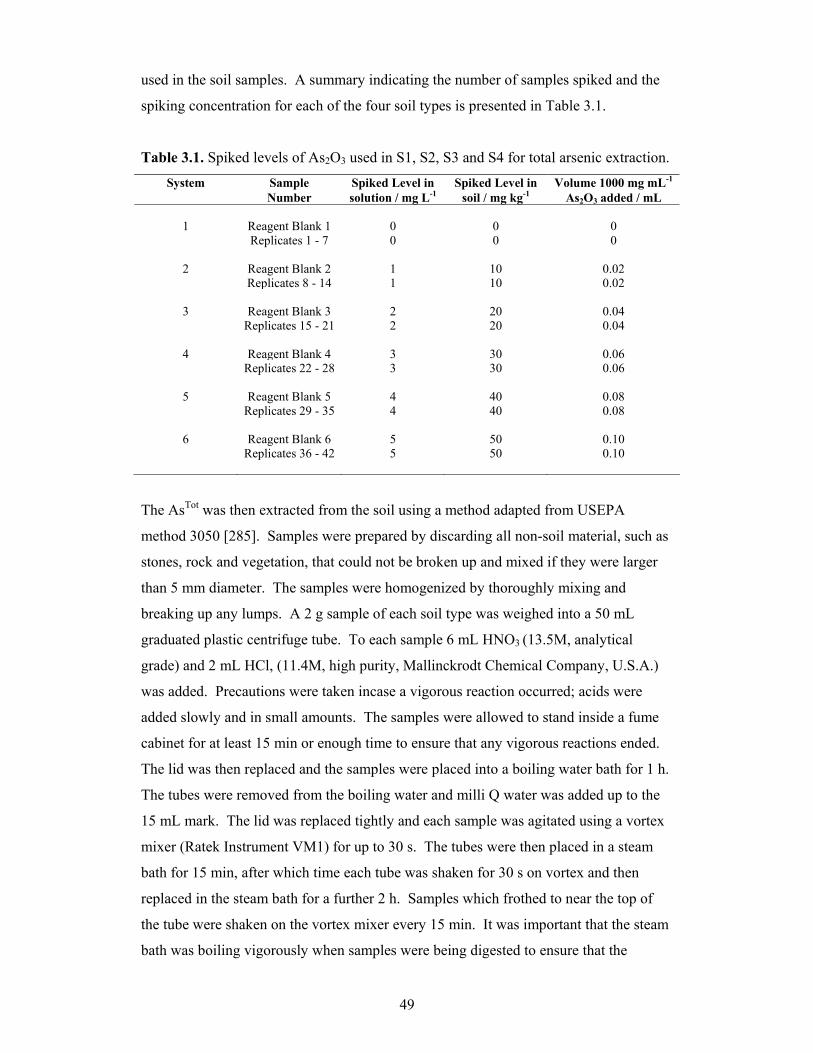
49
used in the soil samples. A summary indicating the number of samples spiked and the
spiking concentration for each of the four soil types is presented in Table 3.1.
Table 3.1. Spiked levels of As2O3 used in S1, S2, S3 and S4 for total arsenic extraction.
System Sample Spiked Level in Spiked Level in Volume 1000 mg mL-1 Number solution / mg L-1 soil / mg kg-1 As2O3 added / mL
1 Reagent Blank 1 0 0 0 Replicates 1 - 7 0 0 0
2 Reagent Blank 2 1 10 0.02 Replicates 8 - 14 1 10 0.02
3 Reagent Blank 3 2 20 0.04 Replicates 15 - 21 2 20 0.04
4 Reagent Blank 4 3 30 0.06 Replicates 22 - 28 3 30 0.06
5 Reagent Blank 5 4 40 0.08 Replicates 29 - 35 4 40 0.08
6 Reagent Blank 6 5 50 0.10 Replicates 36 - 42 5 50 0.10
The AsTot was then extracted from the soil using a method adapted from USEPA
method 3050 [285]. Samples were prepared by discarding all non-soil material, such as
stones, rock and vegetation, that could not be broken up and mixed if they were larger
than 5 mm diameter. The samples were homogenized by thoroughly mixing and
breaking up any lumps. A 2 g sample of each soil type was weighed into a 50 mL
graduated plastic centrifuge tube. To each sample 6 mL HNO3 (13.5M, analytical
grade) and 2 mL HCl, (11.4M, high purity, Mallinckrodt Chemical Company, U.S.A.)
was added. Precautions were taken incase a vigorous reaction occurred; acids were
added slowly and in small amounts. The samples were allowed to stand inside a fume
cabinet for at least 15 min or enough time to ensure that any vigorous reactions ended.
The lid was then replaced and the samples were placed into a boiling water bath for 1 h.
The tubes were removed from the boiling water and milli Q water was added up to the
15 mL mark. The lid was replaced tightly and each sample was agitated using a vortex
mixer (Ratek Instrument VM1) for up to 30 s. The tubes were then placed in a steam
bath for 15 min, after which time each tube was shaken for 30 s on vortex and then
replaced in the steam bath for a further 2 h. Samples which frothed to near the top of
the tube were shaken on the vortex mixer every 15 min. It was important that the steam
bath was boiling vigorously when samples were being digested to ensure that the
50
digesting process was working in the approved manner. The solutions were made up to
the 20 mL mark with Milli Q water and mixed by shaking. All samples were then
centrifuged for 10 min at 1500 r.p.m. The As Tot content of each sample was
determined using an ICP-AES, Perkin Elmer, Optima 4300 DV with CETAC
Technologies ASX – 500 model No. 510 auto-sampler). The ICP-AES used an Rf
power of 1400 W, outer gas flow of 15 L min-1, intermediate gas flow of 0.5 L min-1,
nebulizer gas flow of 0.65 L min-1 using argon gas, sample flow rate of 1.5 mL min-1,
instrument operating pressure was at normal atmospheric pressure (760 mm Hg) and the
temperature was maintained at 21°C.
Total Fe and Al were also extracted from the soil samples using the same method
described above [285]. The extracted Fe and Al concentrations were obtained from the
preliminary As2O3 spiking experiment for the samples which did not contain any spiked
As2O3. The extracted Fe and Al were also used to characterize each of the soil types.
An additional AsTot soil sorption test method was also conducted using the four soil
types – (S1, S2, S3 and S4), however, a different spiking method was used for this
experiment. A 10 mg L-1 stock solution of arsenic trioxide (As2O3, 99.8%, Hopkin &
Williams Limited) solution was made up in a 1 L volumetric flask with analytical grade
milli Q water. A 2 g sample of each of the soil types (each conducted in duplicate) was
weighed into a 50 mL graduated plastic centrifuge tube and made up to the 20 mL mark
with the As2O3 stock solution. Each of the samples was mixed for 30 min on a rotating
mixer and then left to soak for 168 h. Each sample was centrifuged for 15 min at 3000
r.p.m. after which the supernatant solution was decanted and discarded. The soil
samples were washed with 20 mL of milli Q water, mixed for 5 min on a rotating mixer
and then centrifuged for 15 min at 3000 r.p.m. The same washing procedure was
repeated a second time. The soil samples were then extracted using the method adapted
from USEPA method 3050 [285] to determine the AsTot sorbed by the soil. The
extraction and determination (using ICP-AES) procedure are both described above.
3.2.2 Temporal Studies of the Sorption of Arsenic
A temporal AsTot soil sorption test method was also conducted using soil type - S2. A
10 mg L-1 stock solution of As2O3 solution was made up in a 1 L volumetric flask and
made up to the mark with analytical grade milli Q water. Samples (2 g) of type S2 soil
51
were weighed into four separate 50 mL graduated plastic centrifuge tubes and each
made up to the 20 mL mark with the As2O3 stock solution. Each of the samples was
mixed for 30 min on a rotating mixer and then left to soak for 0.5, 24, 48 or 168 h.
Each sample was then centrifuged for 15 min at 3000 r.p.m. after which the supernatant
solution was decanted and discarded. The soil samples were washed with 20 mL of
milli Q water, mixed for 5 min on a rotating mixer and then centrifuged for 15 min at
3000 r.p.m. The same washing procedure was repeated a second time. The soil
samples were then extracted using the method adapted from USEPA method 3050 [285]
to determine the AsTot sorbed by the soil. The extraction and determination (using ICP-
AES) procedure are both described in Section 3.2.1.
3.3 Bioavailability using Geophagy Method
An experiment was conducted to estimate the proportion of AsTot that would be
potentially made available (i.e. bioavailable) to the human body. The bioavailability
method used in this experiment is adapted from the geophagy digestion or “gut”
simulation method [134-135] that has been used in the past to determine the nutrients
made available to humans from eating clay. The bioavailability experiment was
conducted on the same four soil types as specified previously in Section 3.2 – S1, S2,
S3 and S4. The experiment involved spiking each of the soil types at various arsenic
concentrations using a 1000 µg mL-1 As2O3 (99.99%, Perkin Elmer Australia) aqueous
solution. The spiking was conducted by adding a quantity of As2O3 into the soil sample
using an auto-pipette. Each soil type was spiked using six different As2O3 solutions (0,
1, 2, 3, 4 and 5 mg L-1) with each concentration conducted in seven replicates. Six
reagent blank spikes were also prepared and consisted of samples containing no soil that
were spiked at the same As2O3 concentrations as those used in the soil samples. A
summary indicating the number of samples spiked and the spiking concentration for
each of the four soil types is presented in Table 3.2.
The bioavailable AsTot was then extracted from the soil using the adapted geophagy
“gut” simulation method [134-135]. Samples were prepared by discarding all non-soil
material, such as, stones, rock and vegetation that was larger than 5 mm diameter and
that could not be broken up and mixed. Any large matter that remained in the samples
was broken up and the samples were homogenized by thoroughly mixing. A 0.5 g
sample of each soil type was weighed into a 50 mL graduated plastic centrifuge tube.
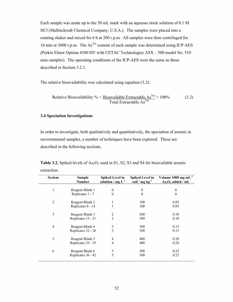
52
Each sample was made up to the 50 mL mark with an aqueous stock solution of 0.1 M
HCl (Mallinckrodt Chemical Company, U.S.A.). The samples were placed into a
rotating shaker and mixed for 6 h at 200 r.p.m. All samples were then centrifuged for
10 min at 3000 r.p.m. The AsTot content of each sample was determined using ICP-AES
(Perkin Elmer Optima 4300 DV with CETAC Technologies ASX – 500 model No. 510
auto-sampler). The operating conditions of the ICP-AES were the same as those
described in Section 3.2.1.
The relative bioavailability was calculated using equation (3.2):
Relative Bioavailability % = Bioavailable Extractable AsTot × 100% (3.2) Total Extractable AsTot
3.4 Speciation Investigations
In order to investigate, both qualitatively and quantitatively, the speciation of arsenic in
environmental samples, a number of techniques have been explored. These are
described in the following sections.
Table 3.2. Spiked levels of As2O3 used in S1, S2, S3 and S4 for bioavailable arsenic
extraction. System Sample Spiked Level in Spiked Level in Volume 1000 mg mL-1
Number solution / mg L-1 soil / mg kg-1 As2O3 added / mL
1 Reagent Blank 1 0 0 0 Replicates 1 - 7 0 0 0
2 Reagent Blank 2 1 100 0.05 Replicates 8 - 14 1 100 0.05
3 Reagent Blank 3 2 200 0.10 Replicates 15 - 21 2 200 0.10
4 Reagent Blank 4 3 300 0.15 Replicates 22 - 28 3 300 0.15
5 Reagent Blank 5 4 400 0.20 Replicates 29 - 35 4 400 0.20
6 Reagent Blank 6 5 500 0.25 Replicates 36 - 42 5 500 0.25
53
3.4.1 Electrospray Mass Spectrometry of Phosphorus and Arsenic Species
Investigations were performed to explore the utility of ESI-MS for the characterization
of arsenic species in solution. Parallel investigations were also undertaken on
phosphorus species as a benchmark, since the chemistries of arsenic and phosphorus are
closely related and phosphorus chemistry is better characterized in the literature [286-
288]. Aqueous stock solutions of the sodium salts of arsenate, arsenite and phosphate
were made up at concentrations of 20 mg L-1 in three separate 1 L volumetric flasks.
Each of the volumetric flasks was made up to the mark with analytical grade Milli-Q
water. The arsenate and arsenite stock solutions were made up using di-sodium
hydrogen arsenate heptahydrate (Na2HAsO4.7H2O, 98.0%, Sigma Chemical Company)
and sodium meta arsenite (NaAsO2, 99.0%, Sigma Chemical Company) respectively.
Anhydrous di-sodium hydrogen orthophosphate (Na2HPO4, 98 to 100.5%, BDH
Chemicals Ltd) was used for the phosphate stock solution.
Each of the stock solutions was further diluted to 1 mg L-1 with Milli-Q water for use in
the ESI-MS. The 1 mg L-1 aqueous solutions of arsenate, arsenite and phosphate were
individually injected directly into the ESI-MS using a 50 µL glass syringe with a
stainless steel needle. Mass analysis was performed using a Micromass Platform II
8326E Electrospray Mass-Spectrometer using a Windows NT version 3.51 running on a
personal computer. The software used was the Masslynx NT, version 2.22. The ESI-
MS source temperature was 20°C, turbo pressure 1.0 x 10⁻⁶ mBar; nitrogen was used as
the nebulizing gas (10 L h-1). The electrospray potential was set to 3 kV in both positive
and negative ion modes and the extraction cone voltage was usually 30 V unless stated
otherwise. It has been demonstrated that lower cone voltages (i.e. ≤ 30 V) are required
to preserve dissolved-phase interactions [289]. The 50 µL aliquots were introduced into
a mobile phase of 90% v/v tetrahydrofuran (THF, 99.0%, Sigma Chemical Company) at
a flow rate of 20 µL min-1. Mass spectral acquisition was usually performed from m/z =
0 to m/z = 250 in 10 s.
3.4.2 Computer Modelling of ESI-MS Identified Phosphorus and Arsenic Species
The equilibrium geometries and relative energies of all relevant phosphorus and arsenic
species identified in the ESI-MS spectra (see Table 4.7) were calculated under high
level density functional theory (DFT); namely B3LYP, using the diffuse basis set 6-
54
311+G** [290]. This level of calculation was chosen since the individual calculated
energies have been employed to determine the energies for postulated reactions
involving a number of these species and it is therefore important for the effects of
electron correlation to be taken into account. The diffuse basis set was chosen since
most of the species under investigation are anionic for which a description of electron
distributions far away from atomic positions should be accommodated [290]. The
software used was Spartan ‘04 Windows (Version 1.0.1, Wavefunction Inc., 18401
Von, Irvine CA 92612 USA). All calculations were performed on standard laptop
computers (Toshiba Satellite Pro and P20). From the calculations, a variety of
additional information on these species may be obtained, including, molecular
structures, formation energies, bond angles, bond lengths, conventional space-filling
volume and area, weight, energy of the highest occupied molecular orbital (EHOMO),
energy of the lowest unoccupied molecular orbital (ELUMO), dipole, electrostatic charge
structures, electrostatic potential energy maps, HOMO structures and LUMO structures
(see Table 4.7, Chart 4.1, 4.2, 4.4 and 4.5). The output files for these calculations are
available on the attached CD.
3.4.3 Selective Organic Phase Extraction of AsIII from Soil
The arsenic speciation method utilized in this investigation was chosen because it was
desirable to quantitatively speciate all of the arsenic present in selected soil samples
using a simple procedure. The method involves extracting the arsenic from the soil with
concentrated hydrochloric acid and to speciate using solvent extractions. The method
works on the premise that AsIII can be selectively extracted into an organic phase from a
strongly acidic phase and is then back-extracted into water for analysis [29,264-265]. It
has been shown that inorganic arsenic in solution is most stable in its hydrolysed form
[263], however, in the presence of an excess of hydrochloric acid, chlorination of
arsenic will occur, yielding arsenic trichloride and arsenic pentachloride. It has also
been shown that arsenic trichloride is a covalent molecule while arsenic pentachloride
most likely exists as the complex ions, [AsCl4]+ or [AsCl6]¯ [263]. The arsenic
trichloride can be extracted into an organic phase such as chloroform or benzene, while
AsV is excluded owing to its ionic properties. The AsIII contained in the organic phase
can be easily recovered by back extraction with water, since inorganic arsenic is most
stable in solution in its hydrolysed form. When the AsIII comes into contact with water,
hydrolysis occurs, excluding the arsenic from the organic phase [32].
55
This arsenic speciation method was first implemented to standardize an arsenite sample
and then used to determine the amount of AsIII sorbed onto soil at different pH levels.
3.4.3.1 Method for the Standardisation of Arsenite Sample
Three separate aqueous stock solutions were made-up containing the following arsenic
species: (i) 76.7 mg L-1 AsIII as NaAsO2, (ii) 55.1 mg L-1 AsV as Na2AsO4.7H2O, and
(iii) 50% v/v mixture of the AsIII and AsV stock solutions. Analytical grade milli-Q
water was used to dilute each of the solutions. Determination of AsIII was conducted in
the following way. A 10 mL aliquot of each of the stock solutions was transferred into
three separate 100 mL separating funnels and 80 mL of 10 M HCl (high purity,
Mallinckrodt Chemical Company, U.S.A.) was then added to each separating funnel to
adjust the acid concentration to greater than 9 M. This was followed by extraction of
the AsIII into chloroform with 4 × 10 mL washings. At that stage the strongly acidic
aqueous phase (i.e. top layer) was discarded. The AsIII was then back-extracted from
the organic phase into 2 × 20 mL aliquots of water and diluted to 100 mL. Each of the
three samples were analyzed using an ICP-AES, Perkin Elmer Optima 4300 DV with
CETAC Technologies ASX – 500 model No. 510 auto-sampler). The ICP-AES
analysis used an Rf power of 1400 W, outer gas flow of 15 L min-1, intermediate gas
flow of 0.5 L min-1, nebulizer gas flow of 0.65 L min-1 using argon gas, sample flow
rate of 1.5 mL min-1, instrument operating pressure at normal atmospheric pressure (760
mm Hg) and the temperature was maintained at 21°C.
The AsTot was also determined by running the three aqueous stock solutions individually
through the ICP-AES. The concentration of AsV was calculated by subtracting the AsIII
concentration from the AsTot. A percent difference from the AsTot was calculated by
taking the difference of AsTot from AsIII and then dividing by the AsTot concentration.
The percent difference is the amount of arsenic which most likely relates to the
oxidative impurities present in the sample container.
3.4.3.2 Method for Arsenite Sorbed onto Soil at Different pH Values
The first part of this experiment involves allowing the sorption of arsenic onto soil
samples. This was achieved using the same three stock solutions that were prepared in
56
Section 3.4.3.1. The pH of the stock solution was adjusted by pouring 50 mL of the
NaAsO2 aqueous stock solution into 5 separate beakers and adjusting the pH in each of
the beakers to pH values of approximately 2, 4, 6.5, 9 and 12 respectively using 0.1 to
1.0 M H2SO4 and 0.1 to 1.0 M NaOH. Where appropriate, throughout this work, pH
measurements were made repeatedly to ensure that the pH of the medium remained
constant.
A 5 g soil sample (light clay - S2) was placed into six separate plastic 50 mL centrifuge
tubes. Five of these centrifuge tubes containing the pre-weighed soil sample were made
up to the 50 mL mark using the pH-adjusted stock solutions. The sixth centrifuge tube
was made up to the 50 mL mark with analytical grade milli-Q water (blank H2O). The
contents of each of the six tubes was mixed on a rotating mixer for 30 min and then left
to soak for 7 days. The samples were centrifuged for 15 min at 3000 r.p.m. and
decanted. The supernatant liquid from the decanting was retained for later use. Each
soil sample was washed with 20 mL milli-Q water, mixed for 5 min on a rotating mixer,
centrifuged for 15 min at 3000 r.p.m. and decanted. The washing procedure was
repeated a second time.
The next part of the experiment involved the extraction of AsTot from the soil. This
involved treating each of the six samples with a 20 mL aliquot of 10 M HCl, and
shaking it vigorously for 30 min. Each sample tube was centrifuged for 5 min at 3000
r.p.m. and poured into a 100 mL volumetric flask. The AsTot extraction procedure was
repeated two more times (i.e. another 2 × 20 mL of 10 M HCl). The soil sample was
then washed into filter paper (Whatman 44) with milli-Q water and diluted to the 100
mL mark. The concentration of the AsIII species was determined in each sample by
taking a 10 mL aliquot of the AsTot extract and transferring it to a 100 mL separating
funnel where 80 mL of 10 M HCl was added. The AsIII was extracted with 4 × 10 mL
washings of chloroform. The acidic aqueous phase was discarded. The AsIII was then
back-extracted from the organic phase using 2 × 20 mL aliquots of milli-Q water and
diluted to the 100 mL mark in a volumetric flask. Each of the 6 samples was then
analysed by ICP-AES.
The final part of the experiment involved determining the AsIII concentration in the
supernatant liquid for each of the six samples. The AsIII concentration was determined
by taking a 10 mL aliquot of each of the supernatant liquids and transferring each
57
aliquot to a 100 mL separating funnel. To each of the tubes, 80 mL of 10 M HCl was
added. The AsIII was extracted using 4 × 10 mL washings of chloroform. The acidic
aqueous phase was discarded. The AsIII was back-extracted from the organic phase
using 2 × 20 mL aliquots of milli-Q water and diluted to the 100 mL mark in a
volumetric flask. Each of the supernatant liquid samples was then analysed by ICP-
AES.
The whole procedure was repeated two more times, changing the original 76.7 mg L-1
AsIII as NaAsO2 aqueous stock solution to: (i) the previously prepared aqueous stock
solution of 55.1 mg L-1 AsV as Na2AsO4.7H2O; and (ii) the previously prepared aqueous
stock solution containing 50% v/v mixture of the AsIII and AsV stock solutions.
In Sections 3.2, 3.3 and 3.4, where time and resources permitted, replicates and
reference soil material were used for QA/QC purposes. Results for QA/QC have been
included on the appended CD. The preparation of fresh stock solutions of particular
arsenic species was carried out for each experimental section in order to minimize
possible transformation of arsenic between different forms.
58
4.0 Results and Discussion
4.1 Inorganic Background Soil Data
A summary of results for inorganic background soil data is presented in Appendix B.
The summary comprises a table that includes the statistical data calculated for each
constituent in each of the different geological units encountered in the environmental
audit reports that were used to construct the database. The statistical results for six
metals (As, Cr, Cu, Pb, Ni and Zn) within various geological units from the database are
presented and discussed. The nine geological units include: Quaternary Aeolian (Qpw),
Quaternary Coode Island Silt (Qpy), Quaternary Fluvial (Qrc), Quaternary Paludal
(Qrm), Quaternary Newer Volcanics (Qvn), Silurian Anderson Creek Formation (Sla),
Silurian Dargile Formation (Sud), Tertiary Brighton Group (Tpb), and Older Volcanics
(Tvo).
4.1.1 Arsenic
In Figure 4.1, the median arsenic concentration has been summarised within the nine
different geological units located within Melbourne, Australia1. The data were obtained
from the computer database software. The results in Figure 4.1 indicate the geological
unit Sla has the highest median arsenic concentration at 6.4 mg kg-1 with a maximum of
21.0 mg kg-1. The second highest median arsenic concentration occurs in Sud at 6.0
mg kg-1 with a maximum of 20.0 mg kg-1. Both of these geological units formed in the
Silurian age in a sedimentary marine environment and mainly consist of siltstone and
sandstone [291]. Researchers [7,292] suggest that sedimentary rocks are the parent
materials of many different soils and that during the formation of sedimentary rocks,
arsenic is carried down by precipitation of iron hydroxides and sulfides. These
researchers also indicated that arsenic concentrations in soil derived from sedimentary
rocks may contain 20 to 30 mg kg-1 of arsenic. Other sources [71] suggest that
sandstones and limestones often contain arsenic concentrations of anywhere between
less than 1 to 20 mg kg-1.
1 Figures 4.1 to 4.6 are also represented in Appendix C for comparative purposes.
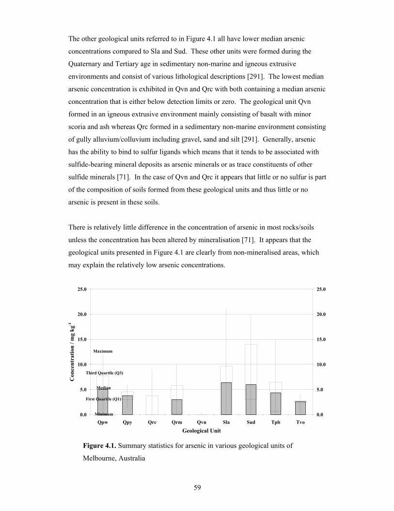
59
The other geological units referred to in Figure 4.1 all have lower median arsenic
concentrations compared to Sla and Sud. These other units were formed during the
Quaternary and Tertiary age in sedimentary non-marine and igneous extrusive
environments and consist of various lithological descriptions [291]. The lowest median
arsenic concentration is exhibited in Qvn and Qrc with both containing a median arsenic
concentration that is either below detection limits or zero. The geological unit Qvn
formed in an igneous extrusive environment mainly consisting of basalt with minor
scoria and ash whereas Qrc formed in a sedimentary non-marine environment consisting
of gully alluvium/colluvium including gravel, sand and silt [291]. Generally, arsenic
has the ability to bind to sulfur ligands which means that it tends to be associated with
sulfide-bearing mineral deposits as arsenic minerals or as trace constituents of other
sulfide minerals [71]. In the case of Qvn and Qrc it appears that little or no sulfur is part
of the composition of soils formed from these geological units and thus little or no
arsenic is present in these soils.
There is relatively little difference in the concentration of arsenic in most rocks/soils
unless the concentration has been altered by mineralisation [71]. It appears that the
geological units presented in Figure 4.1 are clearly from non-mineralised areas, which
may explain the relatively low arsenic concentrations.
0.0
5.0
10.0
15.0
20.0
25.0
Qpw Qpy Qrc Qrm Qvn Sla Sud Tpb Tvo
Geological Unit
Con
cent
ratio
n / m
g kg
-1
0.0
5.0
10.0
15.0
20.0
25.0
Maximum
Minimum
First Quartile (Q1)
Third Quartile (Q3)
Median
Figure 4.1. Summary statistics for arsenic in various geological units of
Melbourne, Australia
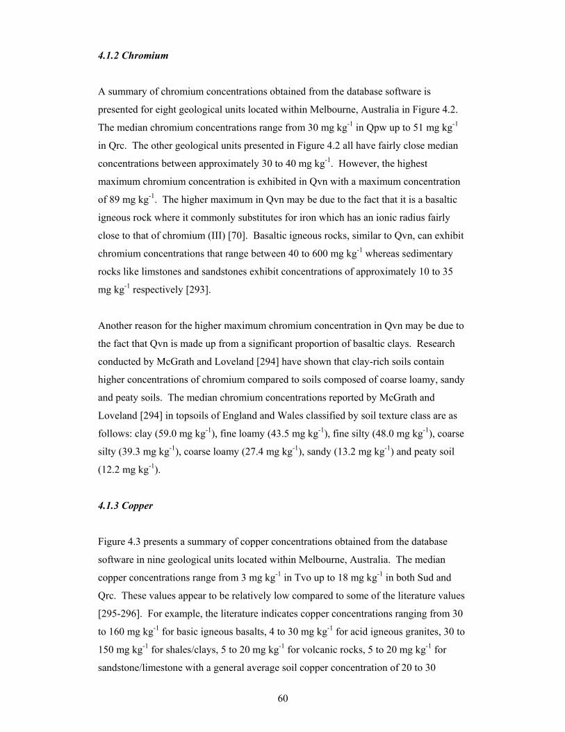
60
4.1.2 Chromium
A summary of chromium concentrations obtained from the database software is
presented for eight geological units located within Melbourne, Australia in Figure 4.2.
The median chromium concentrations range from 30 mg kg-1 in Qpw up to 51 mg kg-1
in Qrc. The other geological units presented in Figure 4.2 all have fairly close median
concentrations between approximately 30 to 40 mg kg-1. However, the highest
maximum chromium concentration is exhibited in Qvn with a maximum concentration
of 89 mg kg-1. The higher maximum in Qvn may be due to the fact that it is a basaltic
igneous rock where it commonly substitutes for iron which has an ionic radius fairly
close to that of chromium (III) [70]. Basaltic igneous rocks, similar to Qvn, can exhibit
chromium concentrations that range between 40 to 600 mg kg-1 whereas sedimentary
rocks like limstones and sandstones exhibit concentrations of approximately 10 to 35
mg kg-1 respectively [293].
Another reason for the higher maximum chromium concentration in Qvn may be due to
the fact that Qvn is made up from a significant proportion of basaltic clays. Research
conducted by McGrath and Loveland [294] have shown that clay-rich soils contain
higher concentrations of chromium compared to soils composed of coarse loamy, sandy
and peaty soils. The median chromium concentrations reported by McGrath and
Loveland [294] in topsoils of England and Wales classified by soil texture class are as
follows: clay (59.0 mg kg-1), fine loamy (43.5 mg kg-1), fine silty (48.0 mg kg-1), coarse
silty (39.3 mg kg-1), coarse loamy (27.4 mg kg-1), sandy (13.2 mg kg-1) and peaty soil
(12.2 mg kg-1).
4.1.3 Copper
Figure 4.3 presents a summary of copper concentrations obtained from the database
software in nine geological units located within Melbourne, Australia. The median
copper concentrations range from 3 mg kg-1 in Tvo up to 18 mg kg-1 in both Sud and
Qrc. These values appear to be relatively low compared to some of the literature values
[295-296]. For example, the literature indicates copper concentrations ranging from 30
to 160 mg kg-1 for basic igneous basalts, 4 to 30 mg kg-1 for acid igneous granites, 30 to
150 mg kg-1 for shales/clays, 5 to 20 mg kg-1 for volcanic rocks, 5 to 20 mg kg-1 for
sandstone/limestone with a general average soil copper concentration of 20 to 30
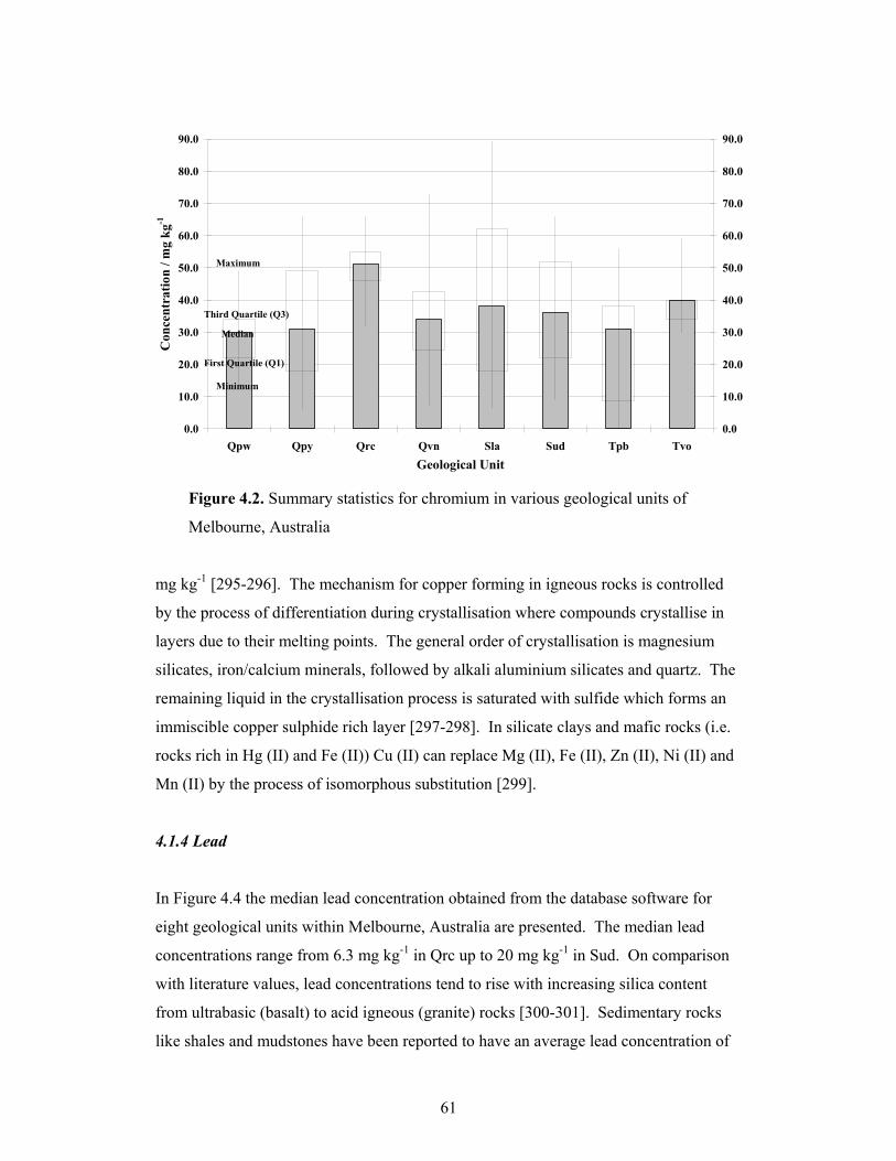
61
0.0
10.0
20.0
30.0
40.0
50.0
60.0
70.0
80.0
90.0
Qpw Qpy Qrc Qvn Sla Sud Tpb TvoGeological Unit
Con
cent
ratio
n / m
g kg
-1
0.0
10.0
20.0
30.0
40.0
50.0
60.0
70.0
80.0
90.0
Maximum
Third Quartile (Q3)
Median
First Quartile (Q1)
Minimum
Figure 4.2. Summary statistics for chromium in various geological units of
Melbourne, Australia
mg kg-1 [295-296]. The mechanism for copper forming in igneous rocks is controlled
by the process of differentiation during crystallisation where compounds crystallise in
layers due to their melting points. The general order of crystallisation is magnesium
silicates, iron/calcium minerals, followed by alkali aluminium silicates and quartz. The
remaining liquid in the crystallisation process is saturated with sulfide which forms an
immiscible copper sulphide rich layer [297-298]. In silicate clays and mafic rocks (i.e.
rocks rich in Hg (II) and Fe (II)) Cu (II) can replace Mg (II), Fe (II), Zn (II), Ni (II) and
Mn (II) by the process of isomorphous substitution [299].
4.1.4 Lead
In Figure 4.4 the median lead concentration obtained from the database software for
eight geological units within Melbourne, Australia are presented. The median lead
concentrations range from 6.3 mg kg-1 in Qrc up to 20 mg kg-1 in Sud. On comparison
with literature values, lead concentrations tend to rise with increasing silica content
from ultrabasic (basalt) to acid igneous (granite) rocks [300-301]. Sedimentary rocks
like shales and mudstones have been reported to have an average lead concentration of
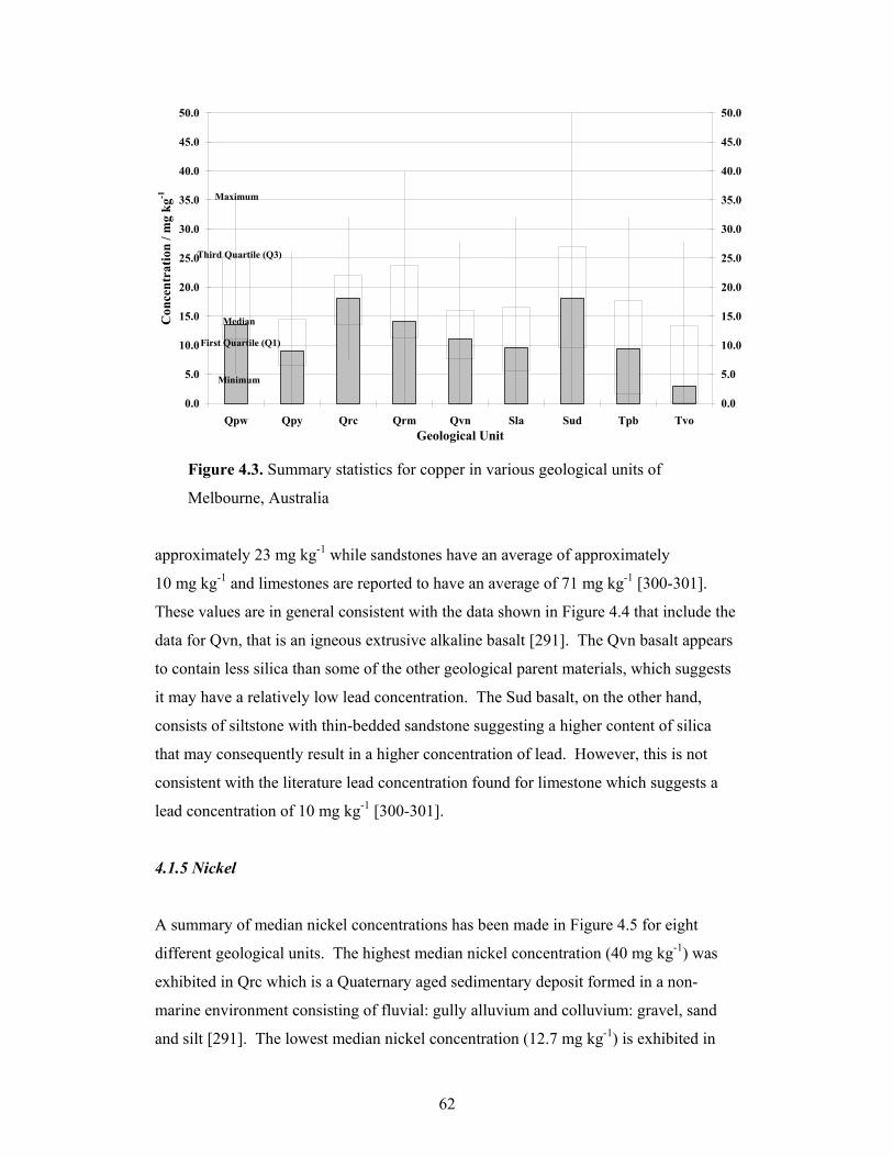
62
0.0
5.0
10.0
15.0
20.0
25.0
30.0
35.0
40.0
45.0
50.0
Qpw Qpy Qrc Qrm Qvn Sla Sud Tpb TvoGeological Unit
Con
cent
ratio
n / m
g kg
-1
0.0
5.0
10.0
15.0
20.0
25.0
30.0
35.0
40.0
45.0
50.0
Maximum
Third Quartile (Q3)
Median
First Quartile (Q1)
Minimum
Figure 4.3. Summary statistics for copper in various geological units of
Melbourne, Australia
approximately 23 mg kg-1 while sandstones have an average of approximately
10 mg kg-1 and limestones are reported to have an average of 71 mg kg-1 [300-301].
These values are in general consistent with the data shown in Figure 4.4 that include the
data for Qvn, that is an igneous extrusive alkaline basalt [291]. The Qvn basalt appears
to contain less silica than some of the other geological parent materials, which suggests
it may have a relatively low lead concentration. The Sud basalt, on the other hand,
consists of siltstone with thin-bedded sandstone suggesting a higher content of silica
that may consequently result in a higher concentration of lead. However, this is not
consistent with the literature lead concentration found for limestone which suggests a
lead concentration of 10 mg kg-1 [300-301].
4.1.5 Nickel
A summary of median nickel concentrations has been made in Figure 4.5 for eight
different geological units. The highest median nickel concentration (40 mg kg-1) was
exhibited in Qrc which is a Quaternary aged sedimentary deposit formed in a non-
marine environment consisting of fluvial: gully alluvium and colluvium: gravel, sand
and silt [291]. The lowest median nickel concentration (12.7 mg kg-1) is exhibited in
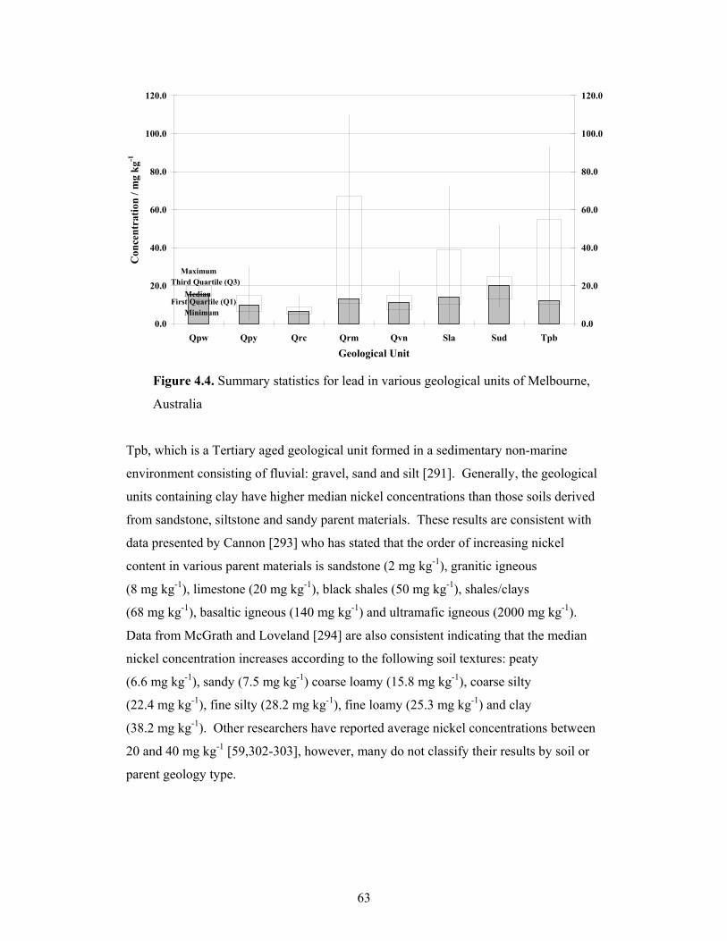
63
0.0
20.0
40.0
60.0
80.0
100.0
120.0
Qpw Qpy Qrc Qrm Qvn Sla Sud Tpb
Geological Unit
Con
cent
ratio
n / m
g kg
-1
0.0
20.0
40.0
60.0
80.0
100.0
120.0
MaximumThird Quartile (Q3)
MedianFirst Quartile (Q1)
Minimum
Figure 4.4. Summary statistics for lead in various geological units of Melbourne,
Australia
Tpb, which is a Tertiary aged geological unit formed in a sedimentary non-marine
environment consisting of fluvial: gravel, sand and silt [291]. Generally, the geological
units containing clay have higher median nickel concentrations than those soils derived
from sandstone, siltstone and sandy parent materials. These results are consistent with
data presented by Cannon [293] who has stated that the order of increasing nickel
content in various parent materials is sandstone (2 mg kg-1), granitic igneous
(8 mg kg-1), limestone (20 mg kg-1), black shales (50 mg kg-1), shales/clays
(68 mg kg-1), basaltic igneous (140 mg kg-1) and ultramafic igneous (2000 mg kg-1).
Data from McGrath and Loveland [294] are also consistent indicating that the median
nickel concentration increases according to the following soil textures: peaty
(6.6 mg kg-1), sandy (7.5 mg kg-1) coarse loamy (15.8 mg kg-1), coarse silty
(22.4 mg kg-1), fine silty (28.2 mg kg-1), fine loamy (25.3 mg kg-1) and clay
(38.2 mg kg-1). Other researchers have reported average nickel concentrations between
20 and 40 mg kg-1 [59,302-303], however, many do not classify their results by soil or
parent geology type.

64
0.0
10.0
20.0
30.0
40.0
50.0
60.0
70.0
80.0
Qpw Qpy Qrc Qvn Sla Sud Tpb TvoGeological Unit
Con
cent
ratio
n / m
g kg
-1
0.0
10.0
20.0
30.0
40.0
50.0
60.0
70.0
80.0
Maximum
Third Quartile (Q3)
Median
First Quartile (Q1)
Minimum
Figure 4.5. Summary statistics for nickel in various geological units of Melbourne,
Australia
4.1.6 Zinc
The median zinc concentrations in nine geological units of Melbourne, Australia range
from 19 to 42 mg kg-1 and the concentrations are summarised in Figure 4.6. The highest
zinc concentration occurs in Qpw which is a Quaternary Pleistocene aged material
which formed in a sedimentary non-marine environment consisting of Aeolian dune
deposits: sand, clay and calcareous sand [291]. The lowest median zinc concentration is
exhibited in Tvo, which is a Tertiary aged material formed in an igneous extrusive
environment consisting of tholeiitic and minor alkaline basalts [291]. Median zinc
concentrations do not vary greatly within the nine geological units and appear to have
relatively low concentrations compared to literature values. Mean zinc contents vary
from 40 mg kg-1 in acid rocks (granites) to 100 mg kg-1 in basaltic rocks [304]. In
sedimentary rocks, the highest zinc contents are found in shales and clayey sediments
(80 to 120 mg kg-1), whereas sandstones, limestones and dolomites generally have lower
contents, ranging from 10 to 30 mg kg-1 [296]. The results summarised in Figure 4.6
appear to be consistent with literature values for sandy materials like sandstones and
limestones [296], however, results for clayey sediments appear to be lower than
expected [296].
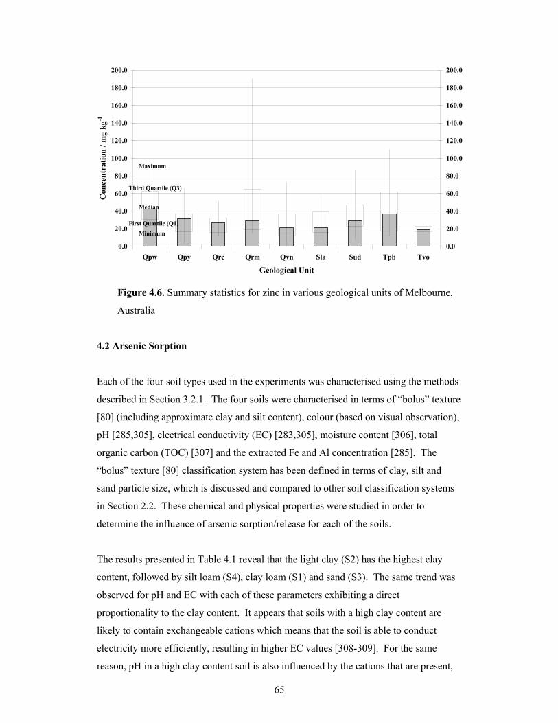
65
0.0
20.0
40.0
60.0
80.0
100.0
120.0
140.0
160.0
180.0
200.0
Qpw Qpy Qrc Qrm Qvn Sla Sud Tpb Tvo
Geological Unit
Con
cent
ratio
n / m
g kg
-1
0.0
20.0
40.0
60.0
80.0
100.0
120.0
140.0
160.0
180.0
200.0
Maximum
Third Quartile (Q3)
Median
First Quartile (Q1)
Minimum
Figure 4.6. Summary statistics for zinc in various geological units of Melbourne,
Australia
4.2 Arsenic Sorption
Each of the four soil types used in the experiments was characterised using the methods
described in Section 3.2.1. The four soils were characterised in terms of “bolus” texture
[80] (including approximate clay and silt content), colour (based on visual observation),
pH [285,305], electrical conductivity (EC) [283,305], moisture content [306], total
organic carbon (TOC) [307] and the extracted Fe and Al concentration [285]. The
“bolus” texture [80] classification system has been defined in terms of clay, silt and
sand particle size, which is discussed and compared to other soil classification systems
in Section 2.2. These chemical and physical properties were studied in order to
determine the influence of arsenic sorption/release for each of the soils.
The results presented in Table 4.1 reveal that the light clay (S2) has the highest clay
content, followed by silt loam (S4), clay loam (S1) and sand (S3). The same trend was
observed for pH and EC with each of these parameters exhibiting a direct
proportionality to the clay content. It appears that soils with a high clay content are
likely to contain exchangeable cations which means that the soil is able to conduct
electricity more efficiently, resulting in higher EC values [308-309]. For the same
reason, pH in a high clay content soil is also influenced by the cations that are present,
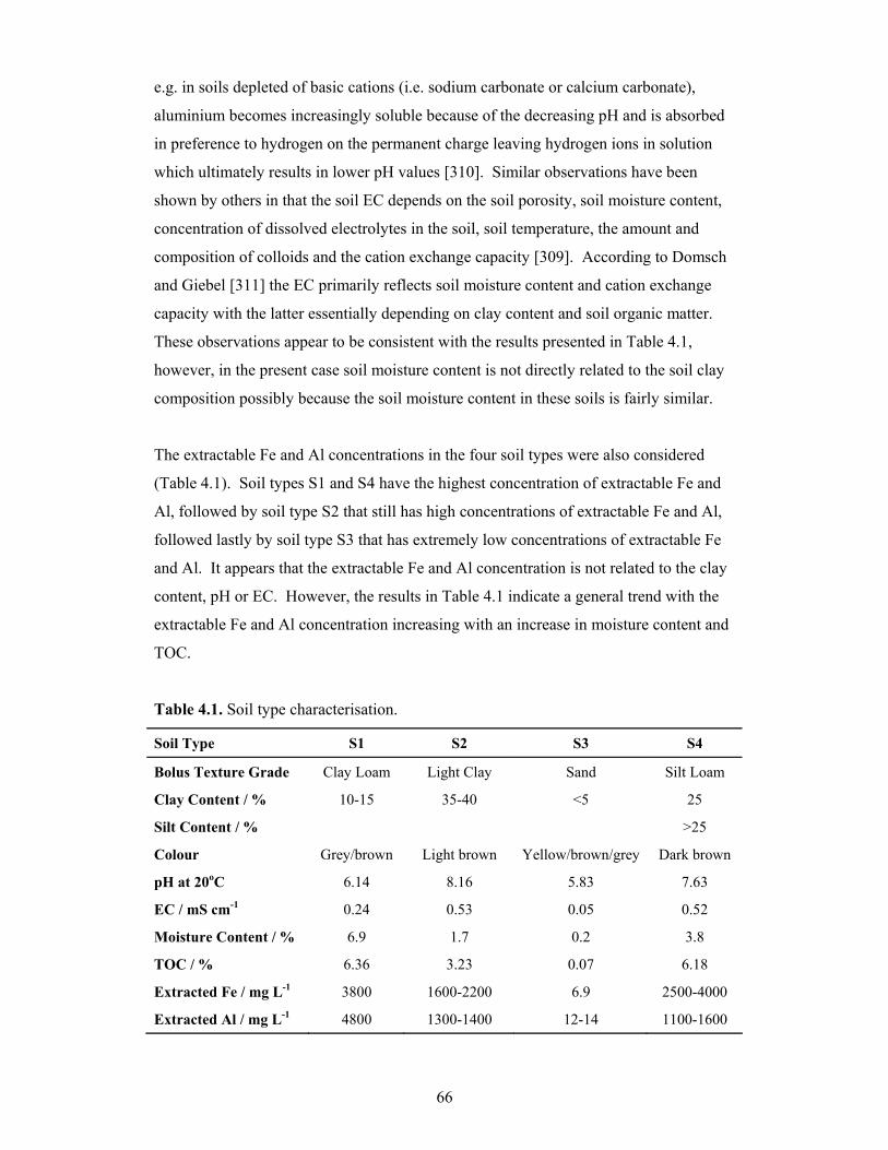
66
e.g. in soils depleted of basic cations (i.e. sodium carbonate or calcium carbonate),
aluminium becomes increasingly soluble because of the decreasing pH and is absorbed
in preference to hydrogen on the permanent charge leaving hydrogen ions in solution
which ultimately results in lower pH values [310]. Similar observations have been
shown by others in that the soil EC depends on the soil porosity, soil moisture content,
concentration of dissolved electrolytes in the soil, soil temperature, the amount and
composition of colloids and the cation exchange capacity [309]. According to Domsch
and Giebel [311] the EC primarily reflects soil moisture content and cation exchange
capacity with the latter essentially depending on clay content and soil organic matter.
These observations appear to be consistent with the results presented in Table 4.1,
however, in the present case soil moisture content is not directly related to the soil clay
composition possibly because the soil moisture content in these soils is fairly similar.
The extractable Fe and Al concentrations in the four soil types were also considered
(Table 4.1). Soil types S1 and S4 have the highest concentration of extractable Fe and
Al, followed by soil type S2 that still has high concentrations of extractable Fe and Al,
followed lastly by soil type S3 that has extremely low concentrations of extractable Fe
and Al. It appears that the extractable Fe and Al concentration is not related to the clay
content, pH or EC. However, the results in Table 4.1 indicate a general trend with the
extractable Fe and Al concentration increasing with an increase in moisture content and
TOC.
Table 4.1. Soil type characterisation.
Soil Type S1 S2 S3 S4
Bolus Texture Grade Clay Loam Light Clay Sand Silt Loam
Clay Content / % 10-15 35-40 <5 25
Silt Content / % >25
Colour Grey/brown Light brown Yellow/brown/grey Dark brown
pH at 20oC 6.14 8.16 5.83 7.63
EC / mS cm-1 0.24 0.53 0.05 0.52
Moisture Content / % 6.9 1.7 0.2 3.8
TOC / % 6.36 3.23 0.07 6.18
Extracted Fe / mg L-1 3800 1600-2200 6.9 2500-4000
Extracted Al / mg L-1 4800 1300-1400 12-14 1100-1600
67
4.2.1 The Effect of Soil Type on As2O3 Sorption
A number of experiments were conducted to determine the effect of soil type on As2O3
sorption. In the first instance a preliminary study was conducted and this is discussed in
Section 4.2.1.1. Further analyses were conducted in Section 4.2.1.2 which involved
altering the spiking method to allow a greater exposure time for the soil to sorb As2O3.
4.2.1.1 Preliminary Study on the Effect of Soil Type on As2O3 Sorption
Having characterized each of the four soil types it was possible to determine in a
preliminary sense, the effect of soil type on the sorption of As2O3. Each of the soil
types was spiked with As2O3 in replicate as described in Section 3.2.1. At each of the
six different spiking levels, the recoverable total arsenic, AsTot, was determined for the
blank sample, AsBlk, as well as the average total arsenic concentration, AsAve, calculated
from seven replicates for each of the four soil types. The standard deviation, AsSt. Dev.,
and the adjusted sample concentration, AsAdj, (i.e. AsAve minus the background
concentration) were calculated. In addition, the percentage of arsenic sorbed by each
soil type, AsTot(sorb), was calculated using Equation 4.1.
%AsTot(sorb) = AsBlk – AsAdj AsBlk
× 100 (4.1)
The average percentage of total arsenic sorbed by each soil type was also calculated by
averaging each of the %AsTot(sorb) values in each of the six systems. The average
percentage %AsTot(sorb) values clearly show that each of the soil types sorbs a different
amount of As2O3 with S1, S2 and S4 having a %AsTot(sorb) of approximately 19.6%,
2.9% and 38.2% respectively. For soil type S3 the value of %AsTot(sorb) is below the
method detection limit. The results for each of the soil types are presented in Table 4.2
and are represented graphically in Figures 4.7 to 4.10 with each discussed in detail
below2.
Figure 4.7 is a plot of the recoverable AsTot concentration versus the spiked As2O3
concentration for soil type S1 and the corresponding blank which contains no soil. It
can be seen that when S1 and the blank are spiked at the same concentration, the clay
2 Figures 4.7 to 4.10 are also represented in Appendix C for comparative purposes.

68
Table 4.2. Effect of soil type on As2O3 sorption.
System Spiked Recoverable Recoverable Recoverable Recoverable [As2O3] AsTot in S1 AsTot in S2 AsTot in S3 AsTot in S4 1 AsBlk / mg L-1 0 0.01 ND 0.01 ND AsAve / mg L-1 0 0.59 0.53 0.04 0.11 AsSt. Dev. / mg L-1 0.08 0.07 0.02 0.05 AsAdj / mg L-1 ND ND ND ND %AsTot(sorb) ND ND ND ND 2 AsBlk / mg L-1 1 0.85 1.04 0.91 1.06 AsAve / mg L-1 1 1.43 1.53 1.15 0.57 AsSt. Dev. / mg L-1 0.18 0.12 0.11 0.08 AsAdj / mg L-1 0.84 0.99 1.11 0.46 %AsTot(sorb) 2.2 4.3 ND 56.8 3 AsBlk / mg L-1 2 2.07 1.99 2.11 1.74 AsAve / mg L-1 2 2.21 2.54 2.20 1.23 AsSt. Dev. / mg L-1 0.09 0.06 0.05 0.09 AsAdj / mg L-1 1.62 2.01 2.16 1.12 %AsTot(sorb) 21.7 ND ND 35.3 4 AsBlk / mg L-1 3 3.15 3.05 3.07 2.99 AsAve / mg L-1 3 2.94 3.54 3.25 2.15 AsSt. Dev. / mg L-1 0.16 0.11 0.08 0.13 AsAdj / mg L-1 2.34 3.01 3.21 2.05 %AsTot(sorb) 25.5 1.5 ND 31.4 5 AsBlk / mg L-1 4 4.26 3.91 4.06 4.13 AsAve / mg L-1 4 3.71 4.55 4.28 2.82 AsSt. Dev. / mg L-1 0.10 0.09 0.13 0.13 AsAdj / mg L-1 3.12 4.02 4.24 2.72 %AsTot(sorb) 26.6 ND ND 34.2 6 AsBlk / mg L-1 5 5.16 4.87 5.02 5.33 AsAve / mg L-1 5 4.61 5.45 5.29 3.66 AsSt. Dev. / mg L-1 0.09 0.20 0.23 0.09 AsAdj / mg L-1 4.02 4.92 5.25 3.56 %AsTot(sorb) 22.1 ND ND 33.3 Average %AsTot(sorb) 19.6 2.9 ND 38.2
Notes: AsTot = total arsenic, AsBlk = arsenic concentration in blank, AsAve = average of the
total arsenic concentration in seven replicates, AsAdj = adjusted AsAve (i.e. AsAve minus
background concentration), AsTot(sorb) = total arsenic sorbed and ND = not detected.
loam has a lower AsTot compared to that of the blank. In addition, as the concentration
of the spike is increased the AsTot concentration in the clay loam decreases compared to
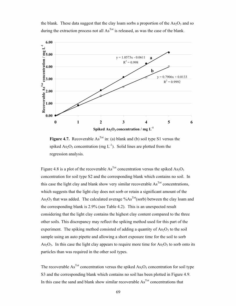
69
the blank. These data suggest that the clay loam sorbs a proportion of the As2O3 and so
during the extraction process not all AsTot is released, as was the case of the blank.
y = 1.0573x - 0.0611R2 = 0.998
y = 0.7906x + 0.0133R2 = 0.9992
0.00
1.00
2.00
3.00
4.00
5.00
6.00
0 1 2 3 4 5 6Spiked As2O3 concentration / mg L-1
Rec
over
able
AsT
ot c
once
ntra
tion
/ mg
L-1
a
b
Figure 4.7. Recoverable AsTot in: (a) blank and (b) soil type S1 versus the
spiked As2O3 concentration (mg L-1). Solid lines are plotted from the
regression analysis.
Figure 4.8 is a plot of the recoverable AsTot concentration versus the spiked As2O3
concentration for soil type S2 and the corresponding blank which contains no soil. In
this case the light clay and blank show very similar recoverable AsTot concentrations,
which suggests that the light clay does not sorb or retain a significant amount of the
As2O3 that was added. The calculated average %AsTot(sorb) between the clay loam and
the corresponding blank is 2.9% (see Table 4.2). This is an unexpected result
considering that the light clay contains the highest clay content compared to the three
other soils. This discrepancy may reflect the spiking method used for this part of the
experiment. The spiking method consisted of adding a quantity of As2O3 to the soil
sample using an auto pipette and allowing a short exposure time for the soil to sorb
As2O3. In this case the light clay appears to require more time for As2O3 to sorb onto its
particles than was required in the other soil types.
The recoverable AsTot concentration versus the spiked As2O3 concentration for soil type
S3 and the corresponding blank which contains no soil has been plotted in Figure 4.9.
In this case the sand and blank show similar recoverable AsTot concentrations that
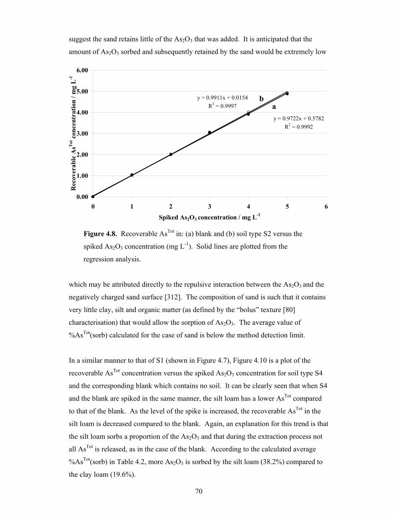
70
suggest the sand retains little of the As2O3 that was added. It is anticipated that the
amount of As2O3 sorbed and subsequently retained by the sand would be extremely low
y = 0.9722x + 0.5782R2 = 0.9992
y = 0.9911x + 0.0154R2 = 0.9997
0.00
1.00
2.00
3.00
4.00
5.00
6.00
0 1 2 3 4 5 6
Spiked As2O3 concentration / mg L-1
Rec
over
able
AsT
ot c
once
ntra
tion
/ mg
L-1
ab
Figure 4.8. Recoverable AsTot in: (a) blank and (b) soil type S2 versus the
spiked As2O3 concentration (mg L-1). Solid lines are plotted from the
regression analysis.
which may be attributed directly to the repulsive interaction between the As2O3 and the
negatively charged sand surface [312]. The composition of sand is such that it contains
very little clay, silt and organic matter (as defined by the “bolus” texture [80]
characterisation) that would allow the sorption of As2O3. The average value of
%AsTot(sorb) calculated for the case of sand is below the method detection limit.
In a similar manner to that of S1 (shown in Figure 4.7), Figure 4.10 is a plot of the
recoverable AsTot concentration versus the spiked As2O3 concentration for soil type S4
and the corresponding blank which contains no soil. It can be clearly seen that when S4
and the blank are spiked in the same manner, the silt loam has a lower AsTot compared
to that of the blank. As the level of the spike is increased, the recoverable AsTot in the
silt loam is decreased compared to the blank. Again, an explanation for this trend is that
the silt loam sorbs a proportion of the As2O3 and that during the extraction process not
all AsTot is released, as in the case of the blank. According to the calculated average
%AsTot(sorb) in Table 4.2, more As2O3 is sorbed by the silt loam (38.2%) compared to
the clay loam (19.6%).

71
y = 1.0142x - 0.0034R2 = 0.9988
y = 1.0479x + 0.041R2 = 0.9998
0.00
1.00
2.00
3.00
4.00
5.00
6.00
0 1 2 3 4 5 6Spiked As2O3 concentration / mg L-1
Rec
over
able
AsT
ot c
once
ntra
tion
/ mg
L-1
a
b
Figure 4.9. Recoverable AsTot in: (a) blank and (b) soil type S3 versus the
spiked As2O3 concentration (mg L-1). Solid lines are plotted from the
regression analysis.
y = 1.0604x - 0.108R2 = 0.9936
y = 0.728x - 0.169R2 = 0.9921
-1.00
0.00
1.00
2.00
3.00
4.00
5.00
6.00
0 1 2 3 4 5 6
Spiked As2O3 concentration / mg L-1
Rec
over
able
AsT
ot c
once
ntra
tion
/ mg
L-1
a
b
Figure 4.10. Recoverable AsTot in: (a) blank and (b) soil type S4 versus the
spiked As2O3 concentration (mg L-1). Solid lines are plotted from the
regression analysis.
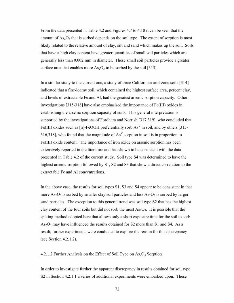
72
From the data presented in Table 4.2 and Figures 4.7 to 4.10 it can be seen that the
amount of As2O3 that is sorbed depends on the soil type. The extent of sorption is most
likely related to the relative amount of clay, silt and sand which makes up the soil. Soils
that have a high clay content have greater quantities of small soil particles which are
generally less than 0.002 mm in diameter. These small soil particles provide a greater
surface area that enables more As2O3 to be sorbed by the soil [313].
In a similar study to the current one, a study of three Californian arid-zone soils [314]
indicated that a fine-loamy soil, which contained the highest surface area, percent clay,
and levels of extractable Fe and Al, had the greatest arsenic sorption capacity. Other
investigations [315-318] have also emphasised the importance of Fe(III) oxides in
establishing the arsenic sorption capacity of soils. This general interpretation is
supported by the investigations of Fordham and Norrish [317,319], who concluded that
Fe(III) oxides such as [α]-FeOOH preferentially sorb AsV in soil, and by others [315-
316,318], who found that the magnitude of AsV sorption in soil is in proportion to
Fe(III) oxide content. The importance of iron oxide on arsenic sorption has been
extensively reported in the literature and has shown to be consistent with the data
presented in Table 4.2 of the current study. Soil type S4 was determined to have the
highest arsenic sorption followed by S1, S2 and S3 that show a direct correlation to the
extractable Fe and Al concentrations.
In the above case, the results for soil types S1, S3 and S4 appear to be consistent in that
more As2O3 is sorbed by smaller clay soil particles and less As2O3 is sorbed by larger
sand particles. The exception to this general trend was soil type S2 that has the highest
clay content of the four soils but did not sorb the most As2O3. It is possible that the
spiking method adopted here that allows only a short exposure time for the soil to sorb
As2O3 may have influenced the results obtained for S2 more than S1 and S4. As a
result, further experiments were conducted to explore the reason for this discrepancy
(see Section 4.2.1.2).
4.2.1.2 Further Analysis on the Effect of Soil Type on As2O3 Sorption
In order to investigate further the apparent discrepancy in results obtained for soil type
S2 in Section 4.2.1.1 a series of additional experiments were embarked upon. These
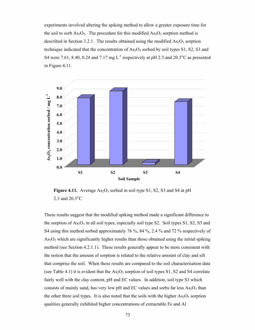
73
experiments involved altering the spiking method to allow a greater exposure time for
the soil to sorb As2O3. The procedure for this modified As2O3 sorption method is
described in Section 3.2.1. The results obtained using the modified As2O3 sorption
technique indicated that the concentration of As2O3 sorbed by soil types S1, S2, S3 and
S4 were 7.61, 8.40, 0.24 and 7.17 mg L-1 respectively at pH 2.3 and 20.3°C as presented
in Figure 4.11.
0.0
1.0
2.0
3.0
4.0
5.0
6.0
7.0
8.0
9.0
As 2
O3 c
once
ntra
tion
sorb
ed /
mg
L-1
S1 S2 S3 S4Soil Sample
Figure 4.11. Average As2O3 sorbed in soil type S1, S2, S3 and S4 at pH
2.3 and 20.3°C
These results suggest that the modified spiking method made a significant difference to
the sorption of As2O3 in all soil types, especially soil type S2. Soil types S1, S2, S3 and
S4 using this method sorbed approximately 76 %, 84 %, 2.4 % and 72 % respectively of
As2O3 which are significantly higher results than those obtained using the initial spiking
method (see Section 4.2.1.1). These results generally appear to be more consistent with
the notion that the amount of sorption is related to the relative amount of clay and silt
that comprise the soil. When these results are compared to the soil characterisation data
(see Table 4.1) it is evident that the As2O3 sorption of soil types S1, S2 and S4 correlate
fairly well with the clay content, pH and EC values. In addition, soil type S3 which
consists of mainly sand, has very low pH and EC values and sorbs far less As2O3 than
the other three soil types. It is also noted that the soils with the higher As2O3 sorption
qualities generally exhibited higher concentrations of extractable Fe and Al
74
concentrations, however, this relationship was not directly related as was the case in the
preliminary experiment (Section 4.2.1.1).
4.2.2 Time Dependency of As2O3 Sorption on Soil
An experiment was conducted to determine the effect of time on the sorption of As2O3
by soil. For this experiment soil type S2 was selected and left to soak in an aqueous
As2O3 solution (10 mg L-1) for time periods 0, 0.5, 24, 48 and 168 h as described in
Section 3.2.2. The results for this experiment indicate that the As2O3 sorption
concentration starts at zero and increases rapidly to 4.74 mg L-1 (C1) after approximately
30 min. After the first 30 min the As2O3 sorption process appears to slow down and
As2O3 continues to be slowly sorbed, approaching a maximum sorption concentration
(C∞). From these observations it is suggested that the sorption process is in fact a two-
step process as represented in Figure 4.12.
0.00
1.00
2.00
3.00
4.00
5.00
6.00
7.00
8.00
9.00
0 20 40 60 80 100 120 140 160 180
Time / h
Sorb
ed A
s 2O
3 / m
g L
-1
a
b
C∞
C1
Figure 4.12. Plot of the sorbed As2O3 versus time showing: (a) the rapid
first-step sorption process and (b) the slower second-step sorption process.
It was decided to test the slower second-step sorption process for first-order kinetic
behaviour. In order to do this it was justifiably assumed that the first sorption process
occurs instantaneously compared with the second process and so the latter process can
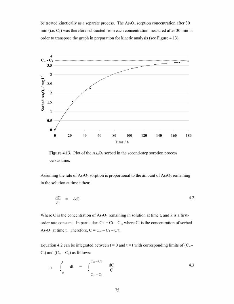
75
be treated kinetically as a separate process. The As2O3 sorption concentration after 30
min (i.e. C1) was therefore subtracted from each concentration measured after 30 min in
order to transpose the graph in preparation for kinetic analysis (see Figure 4.13).
0
0.5
1
1.5
2
2.5
3
3.5
4
0 20 40 60 80 100 120 140 160 180
Time / h
Sorb
ed A
s 2O
3 / m
g L
-1
C∞ - C1
Figure 4.13. Plot of the As2O3 sorbed in the second-step sorption process
versus time.
Assuming the rate of As2O3 sorption is proportional to the amount of As2O3 remaining
in the solution at time t then:
dC dt
= -kC 4.2
Where C is the concentration of As2O3 remaining in solution at time t, and k is a first-
order rate constant. In particular: C′t = Ct – C1, where Ct is the concentration of sorbed
As2O3 at time t. Therefore, C = C∞ – C1 – C′t.
Equation 4.2 can be integrated between t = 0 and t = t with corresponding limits of (C∞–
Ct) and (C∞ – C1) as follows:
-k t
∫ 0
dt = C∞ – Ct
∫ C∞ – C1
dC C
4.3
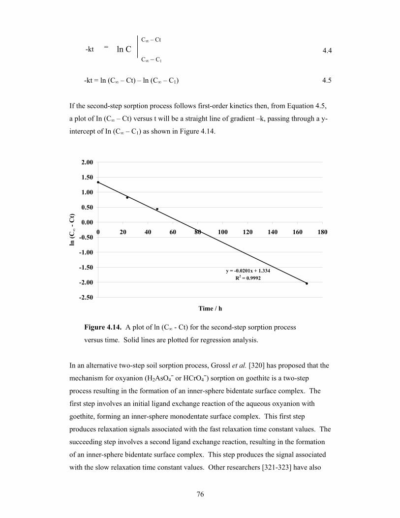
76
-kt = ln C C∞ – Ct
C∞ – C1
4.4
-kt = ln (C∞ – Ct) – ln (C∞ – C1) 4.5
If the second-step sorption process follows first-order kinetics then, from Equation 4.5,
a plot of In (C∞ – Ct) versus t will be a straight line of gradient –k, passing through a y-
intercept of In (C∞ – C1) as shown in Figure 4.14.
y = -0.0201x + 1.334R2 = 0.9992
-2.50
-2.00
-1.50
-1.00
-0.50
0.00
0.50
1.00
1.50
2.00
0 20 40 60 80 100 120 140 160 180
Time / h
ln (C
∞ -
Ct)
Figure 4.14. A plot of ln (C∞ - Ct) for the second-step sorption process
versus time. Solid lines are plotted for regression analysis.
In an alternative two-step soil sorption process, Grossl et al. [320] has proposed that the
mechanism for oxyanion (H2AsO4¯ or HCrO4¯) sorption on goethite is a two-step
process resulting in the formation of an inner-sphere bidentate surface complex. The
first step involves an initial ligand exchange reaction of the aqueous oxyanion with
goethite, forming an inner-sphere monodentate surface complex. This first step
produces relaxation signals associated with the fast relaxation time constant values. The
succeeding step involves a second ligand exchange reaction, resulting in the formation
of an inner-sphere bidentate surface complex. This step produces the signal associated
with the slow relaxation time constant values. Other researchers [321-323] have also

77
reported the formation of inner-sphere bidentate binuclear complexes with the sorption
of HAsO42¯ on iron oxide surfaces analogous to the HPO4
2¯ anion [324]. It would
appear that these results [320] are consistent with the results presented in Figure 4.12 of
the current study.
Raven et al. [95] and Fuller et al. [103] also reported the slow sorption kinetics of
arsenate on ferrihydrite after an initial rapid sorption of 5 min. It was suggested [95]
that the different relative reaction rates at low and high initial arsenic concentrations for
arsenate sorption could relate to Extended X-ray Absorption Fine Structure (EXAFS)
results [322,325-326], which have provided evidence that, at low surface coverage,
arsenate is retained mainly by the formation of monodentate complexes on the iron
oxide surface, and at high surface coverage arsenate binds to the surface mainly by the
formation of bidentate binuclear and bidentate mononuclear complexes. It is possible
that formation of the bidentate complexes at high surface coverage is slower than the
predominantly monodentate reactions at low surface coverage. Raven et al. [95]
indicated that the arsenic sorption kinetic data were generally best described by the
parabolic diffusion equation. The results suggest that the reactions between arsenic and
ferrihydrite were diffusion-controlled. Fuller et al. [103] reported that the time
dependence of arsenate sorption on ferrihydrite could be described by a general model
for diffusion into a sphere if a subset of surface sites located near the exterior of
aggregates is assumed to attain equilibrium rapidly. Orthophosphate diffusion
(analogous to H2AsO4¯) into ferrihydrite particles has been verified by electron
microprobe analysis [327], however, the diffusion of arsenic into ferrihydrite particles
has not been verified.
In a similar experiment [328], it was shown that the removal of AsV, from solution to
soil, increases with time and attains saturation in approximately 35 min for hematite and
approximately 60 min for feldspars with removal occurring rapidly in the initial stages
and decreasing with time. The sorption of AsV onto hematite/feldspar was determined
using mathematical modelling based on first-order kinetics. The same observation was
reported by Smith et al. [329] who indicated that various soils were able to remove AsV
rapidly and attain equilibrium in 1 h and that after the initial rapid removal, sorption of
AsV continued at a slow and steady rate for the 72 h investigation. Other researchers
have also reported similar findings for AsV sorption [316] and AsIII sorption [315,330].
78
4.3 Bioavailability of Arsenic
The bioavailability of AsTot was determined in each of the four soil types as described in
Section 3.4. The method used was adapted from the geophagy digestion method [134-
135] that has been used in the past to determine the nutrients made available to humans
from eating clay. The results for the bioavailability experiment are presented in Table
4.3.
The results indicate that as the concentration of the As2O3 spike increases, the
% AsBioavailability also increases until it reaches a maximum value. Each soil type has
different physical and chemical properties (shown in Table 4.1) which controls the
amount of AsTot bound by the soil. Clearly, the amount of AsTot that is not tightly bound
by the soil is the amount of AsTot that is bioavailable. This applies for soil types S1, S2,
S3 and S4 with the % AsBioavailability approaching approximately 32%, 80%, 100% and
60% respectively. These results show that the composition of soils greatly affects the
% AsBioavailability which means that a 100% AsBioavailability does not occur in the case of
many soils. Studies investigating the sorption of soluble arsenic ingested by humans
suggest that close to 100% of soluble arsenic is sorbed from the gastrointestinal tract
[16,123]. However, arsenic in soils generally exists as mineral forms or soil-arsenic
complexes that will be incompletely solubilised during transit through the
gastrointestinal tract. Research indicates that arsenic must be dissolved in order to be
completely sorbed [124] which means that far less sorption of arsenic will occur from
soil.
It is noted in System 1 of Table 4.3, where no As2O3 spike was added, that the results do
not fit well with the rest of the data. Two plausible explanations for this irregularity are:
(i) the total and bioavailable arsenic concentrations presented in Table 4.2 and Table 4.3
respectively are measured at very low concentrations which are close to the limit of the
ICP-AES detection limit. These values may not be reliable for data analysis purposes
and ultimately may affect the calculated % AsBioavailability; and (ii) that the arsenic present
is the background concentration which may exist as a different species to that of As2O3.
This may affect the % AsBioavailability calculation and, as a result, System 1 data (from
Table 4.3) were not used in data analyses.
79
The results in Table 4.3 indicate that the sorption process is not an equilibrium process
because the calculated ratio (R) of the % AsBioavailability to the % AsNon-bioavailability varies
with the concentration of the As2O3 spike. If these ratios were partition coefficients
they would be expected to remain constant. In particular, the relationship between
% AsBioavailability versus the concentration of As2O3 spike, s, is derived in Equations 4.6
and 4.7.
Let b = % AsBioavailability
Then b/(s – b) = K (4.6)
whence b = [K/(1 + K)] s (4.7)
Thus a plot of % AsBioavailability versus s should give a straight line with slope equal to
K/(1 + K).
A plot of % AsBioavailability versus s for the four soil types has been presented in Figure
4.15. A linear relationship is not obtained (see Figure 4.15) suggesting that the amount
of As2O3 tightly bound to the soil is less than that which occurs at lower spiked
concentrations. This could be due to competition for sorption sites on the soil at higher
As2O3 concentrations.
Moreover, tangents at s = 0 on the plot of % AsBioavailability versus s can be used to
estimate the values of the partition coefficients. The calculated tangent m = K/(1 + K),
so that K = m/(1 – m).
The estimated tangent and the calculated partition coefficient at s = 0 are shown in
Table 4.4.
A study conducted by Oomen et al. [133] compared five in vitro digestion models using
three different soil types to assess the bioaccessibility of As, Pb and Cd. One of the
digestive models evaluated (called the ‘SBET’ method) is similar to the geophagy
digestion method [134-135] in that they both simulate a stomach (gastric) digestion
system that does not take into account the intestinal compartment. These methods are
quite significant for bioavailability studies because they provide an extremely simple
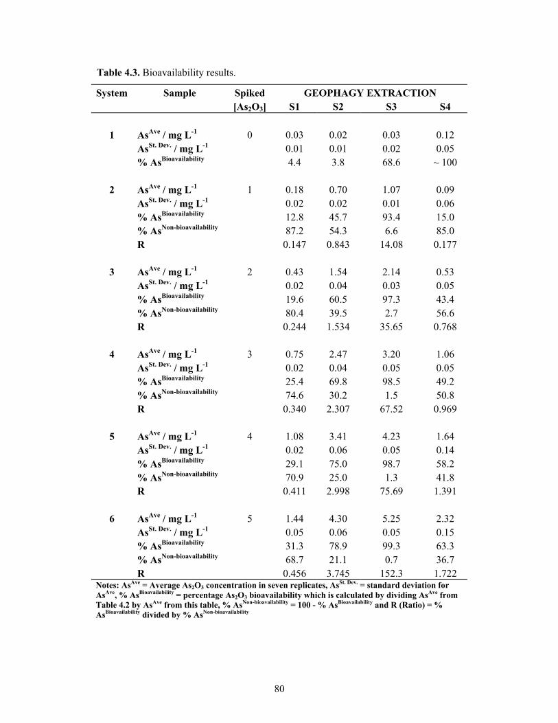
80
Table 4.3. Bioavailability results.
System Sample Spiked GEOPHAGY EXTRACTION [As2O3] S1 S2 S3 S4 1 AsAve / mg L-1 0 0.03 0.02 0.03 0.12 AsSt. Dev. / mg L-1 0.01 0.01 0.02 0.05 % AsBioavailability 4.4 3.8 68.6 ~ 100 2 AsAve / mg L-1 1 0.18 0.70 1.07 0.09 AsSt. Dev. / mg L-1 0.02 0.02 0.01 0.06 % AsBioavailability 12.8 45.7 93.4 15.0 % AsNon-bioavailability 87.2 54.3 6.6 85.0 R 0.147 0.843 14.08 0.177 3 AsAve / mg L-1 2 0.43 1.54 2.14 0.53 AsSt. Dev. / mg L-1 0.02 0.04 0.03 0.05 % AsBioavailability 19.6 60.5 97.3 43.4 % AsNon-bioavailability 80.4 39.5 2.7 56.6 R 0.244 1.534 35.65 0.768 4 AsAve / mg L-1 3 0.75 2.47 3.20 1.06 AsSt. Dev. / mg L-1 0.02 0.04 0.05 0.05 % AsBioavailability 25.4 69.8 98.5 49.2 % AsNon-bioavailability 74.6 30.2 1.5 50.8 R 0.340 2.307 67.52 0.969 5 AsAve / mg L-1 4 1.08 3.41 4.23 1.64 AsSt. Dev. / mg L-1 0.02 0.06 0.05 0.14 % AsBioavailability 29.1 75.0 98.7 58.2 % AsNon-bioavailability 70.9 25.0 1.3 41.8 R 0.411 2.998 75.69 1.391 6 AsAve / mg L-1 5 1.44 4.30 5.25 2.32 AsSt. Dev. / mg L-1 0.05 0.06 0.05 0.15 % AsBioavailability 31.3 78.9 99.3 63.3 % AsNon-bioavailability 68.7 21.1 0.7 36.7 R 0.456 3.745 152.3 1.722
Notes: AsAve = Average As2O3 concentration in seven replicates, AsSt. Dev. = standard deviation for AsAve, % AsBioavailability = percentage As2O3 bioavailability which is calculated by dividing AsAve from Table 4.2 by AsAve from this table, % AsNon-bioavailability = 100 - % AsBioavailability and R (Ratio) = % AsBioavailability divided by % AsNon-bioavailability
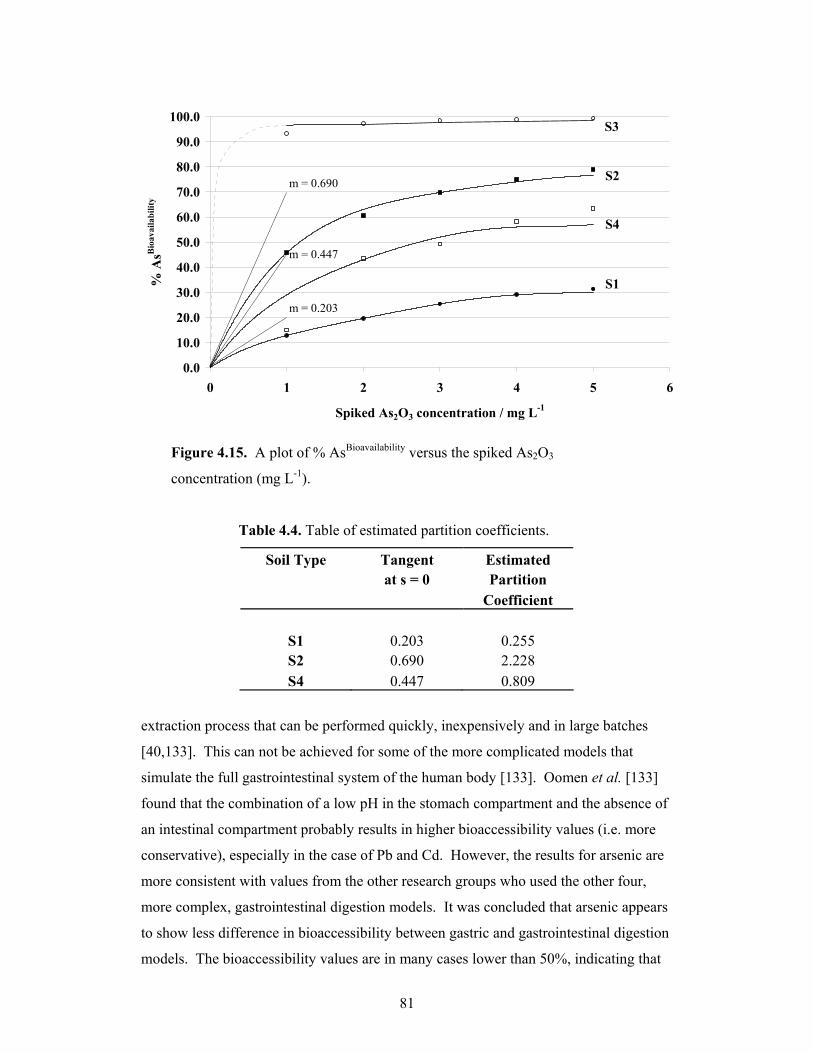
81
0.0
10.0
20.0
30.0
40.0
50.0
60.0
70.0
80.0
90.0
100.0
0 1 2 3 4 5 6
Spiked As2O3 concentration / mg L-1
% A
sBio
avai
labi
lity
S1
S4
S2
S3
m = 0.690
m = 0.447
m = 0.203
Figure 4.15. A plot of % AsBioavailability versus the spiked As2O3
concentration (mg L-1).
Table 4.4. Table of estimated partition coefficients.
Soil Type Tangent Estimated at s = 0 Partition Coefficient
S1 0.203 0.255 S2 0.690 2.228 S4 0.447 0.809
extraction process that can be performed quickly, inexpensively and in large batches
[40,133]. This can not be achieved for some of the more complicated models that
simulate the full gastrointestinal system of the human body [133]. Oomen et al. [133]
found that the combination of a low pH in the stomach compartment and the absence of
an intestinal compartment probably results in higher bioaccessibility values (i.e. more
conservative), especially in the case of Pb and Cd. However, the results for arsenic are
more consistent with values from the other research groups who used the other four,
more complex, gastrointestinal digestion models. It was concluded that arsenic appears
to show less difference in bioaccessibility between gastric and gastrointestinal digestion
models. The bioaccessibility values are in many cases lower than 50%, indicating that
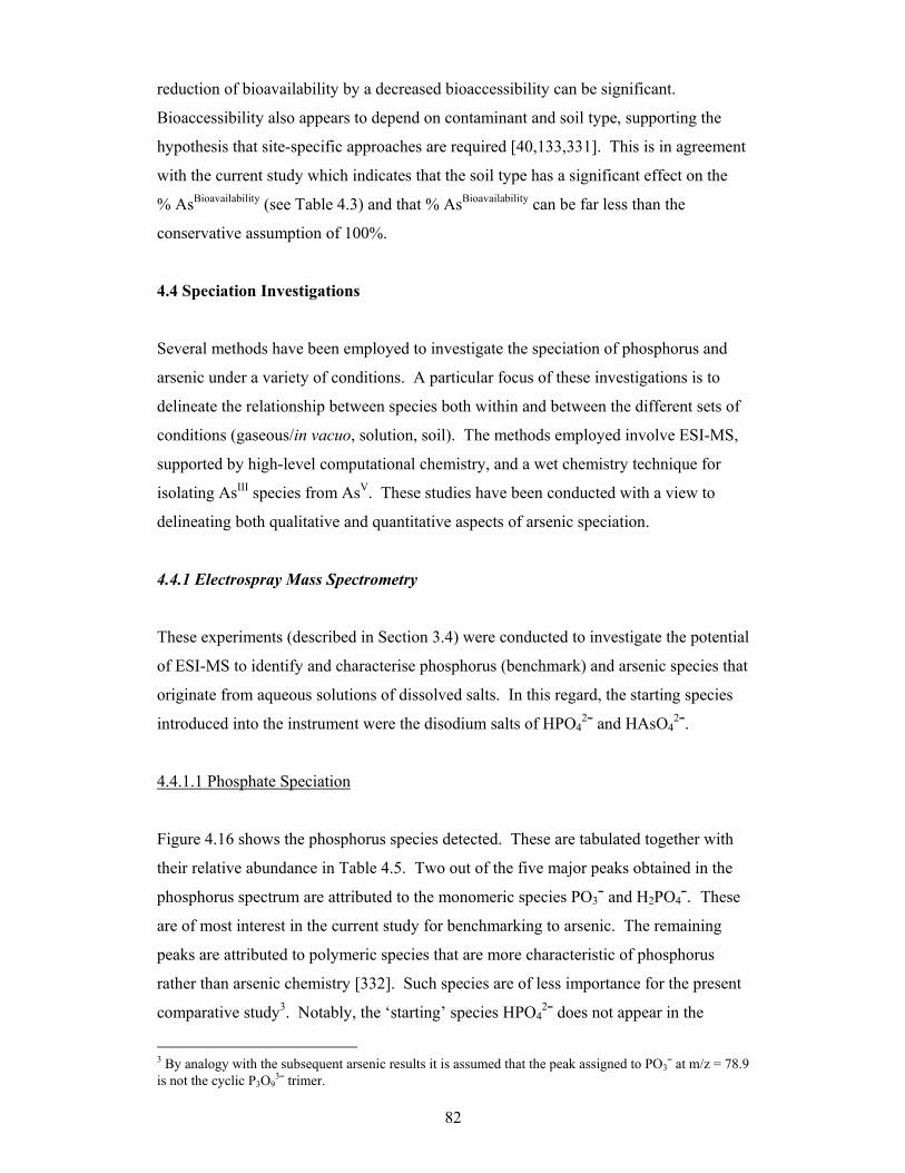
82
reduction of bioavailability by a decreased bioaccessibility can be significant.
Bioaccessibility also appears to depend on contaminant and soil type, supporting the
hypothesis that site-specific approaches are required [40,133,331]. This is in agreement
with the current study which indicates that the soil type has a significant effect on the
% AsBioavailability (see Table 4.3) and that % AsBioavailability can be far less than the
conservative assumption of 100%.
4.4 Speciation Investigations
Several methods have been employed to investigate the speciation of phosphorus and
arsenic under a variety of conditions. A particular focus of these investigations is to
delineate the relationship between species both within and between the different sets of
conditions (gaseous/in vacuo, solution, soil). The methods employed involve ESI-MS,
supported by high-level computational chemistry, and a wet chemistry technique for
isolating AsIII species from AsV. These studies have been conducted with a view to
delineating both qualitative and quantitative aspects of arsenic speciation.
4.4.1 Electrospray Mass Spectrometry
These experiments (described in Section 3.4) were conducted to investigate the potential
of ESI-MS to identify and characterise phosphorus (benchmark) and arsenic species that
originate from aqueous solutions of dissolved salts. In this regard, the starting species
introduced into the instrument were the disodium salts of HPO42¯ and HAsO4
2¯.
4.4.1.1 Phosphate Speciation
Figure 4.16 shows the phosphorus species detected. These are tabulated together with
their relative abundance in Table 4.5. Two out of the five major peaks obtained in the
phosphorus spectrum are attributed to the monomeric species PO3¯ and H2PO4¯. These
are of most interest in the current study for benchmarking to arsenic. The remaining
peaks are attributed to polymeric species that are more characteristic of phosphorus
rather than arsenic chemistry [332]. Such species are of less importance for the present
comparative study3. Notably, the ‘starting’ species HPO42¯ does not appear in the
3 By analogy with the subsequent arsenic results it is assumed that the peak assigned to PO3¯ at m/z = 78.9 is not the cyclic P3O9
3¯ trimer.
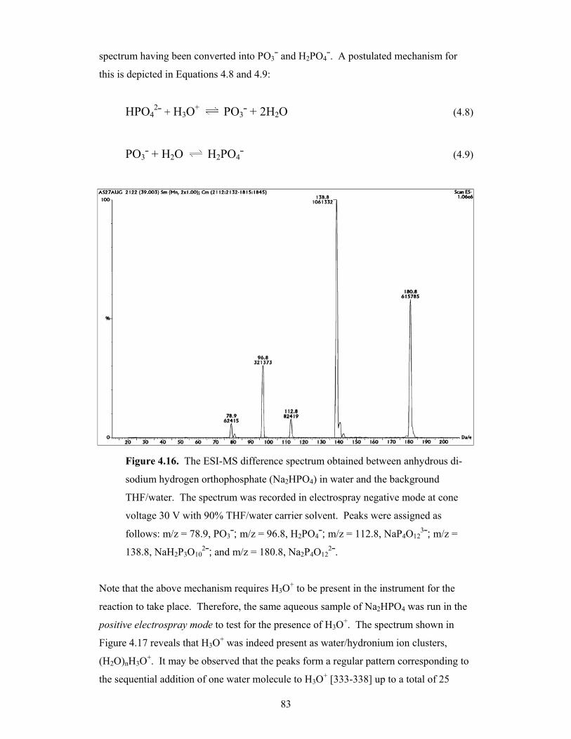
83
spectrum having been converted into PO3¯ and H2PO4¯. A postulated mechanism for
this is depicted in Equations 4.8 and 4.9:
HPO42¯ + H3O+ PO3¯ + 2H2O (4.8)
PO3¯ + H2O H2PO4¯ (4.9)
Figure 4.16. The ESI-MS difference spectrum obtained between anhydrous di-
sodium hydrogen orthophosphate (Na2HPO4) in water and the background
THF/water. The spectrum was recorded in electrospray negative mode at cone
voltage 30 V with 90% THF/water carrier solvent. Peaks were assigned as
follows: m/z = 78.9, PO3¯; m/z = 96.8, H2PO4¯; m/z = 112.8, NaP4O123¯; m/z =
138.8, NaH2P3O102¯; and m/z = 180.8, Na2P4O12
2¯.
Note that the above mechanism requires H3O+ to be present in the instrument for the
reaction to take place. Therefore, the same aqueous sample of Na2HPO4 was run in the
positive electrospray mode to test for the presence of H3O+. The spectrum shown in
Figure 4.17 reveals that H3O+ was indeed present as water/hydronium ion clusters,
(H2O)nH3O+. It may be observed that the peaks form a regular pattern corresponding to
the sequential addition of one water molecule to H3O+ [333-338] up to a total of 25
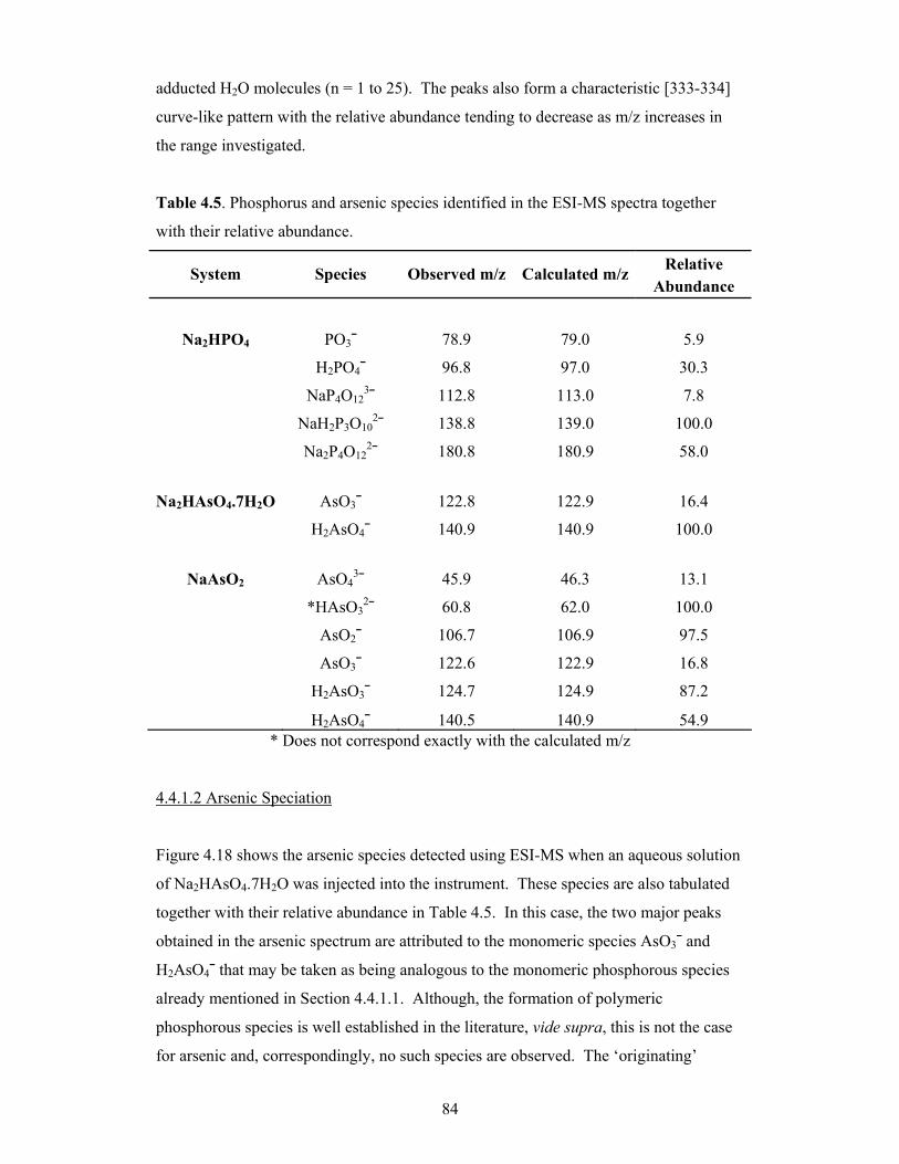
84
adducted H2O molecules (n = 1 to 25). The peaks also form a characteristic [333-334]
curve-like pattern with the relative abundance tending to decrease as m/z increases in
the range investigated.
Table 4.5. Phosphorus and arsenic species identified in the ESI-MS spectra together
with their relative abundance.
Relative System Species Observed m/z Calculated m/zAbundance
Na2HPO4 PO3¯ 78.9 79.0 5.9
H2PO4¯ 96.8 97.0 30.3
NaP4O123¯ 112.8 113.0 7.8
NaH2P3O102¯ 138.8 139.0 100.0
Na2P4O122¯ 180.8 180.9 58.0
Na2HAsO4.7H2O AsO3¯ 122.8 122.9 16.4
H2AsO4¯ 140.9 140.9 100.0
NaAsO2 AsO43¯ 45.9 46.3 13.1
*HAsO32¯ 60.8 62.0 100.0
AsO2¯ 106.7 106.9 97.5
AsO3¯ 122.6 122.9 16.8
H2AsO3¯ 124.7 124.9 87.2
H2AsO4¯ 140.5 140.9 54.9 * Does not correspond exactly with the calculated m/z
4.4.1.2 Arsenic Speciation
Figure 4.18 shows the arsenic species detected using ESI-MS when an aqueous solution
of Na2HAsO4.7H2O was injected into the instrument. These species are also tabulated
together with their relative abundance in Table 4.5. In this case, the two major peaks
obtained in the arsenic spectrum are attributed to the monomeric species AsO3¯ and
H2AsO4¯ that may be taken as being analogous to the monomeric phosphorous species
already mentioned in Section 4.4.1.1. Although, the formation of polymeric
phosphorous species is well established in the literature, vide supra, this is not the case
for arsenic and, correspondingly, no such species are observed. The ‘originating’
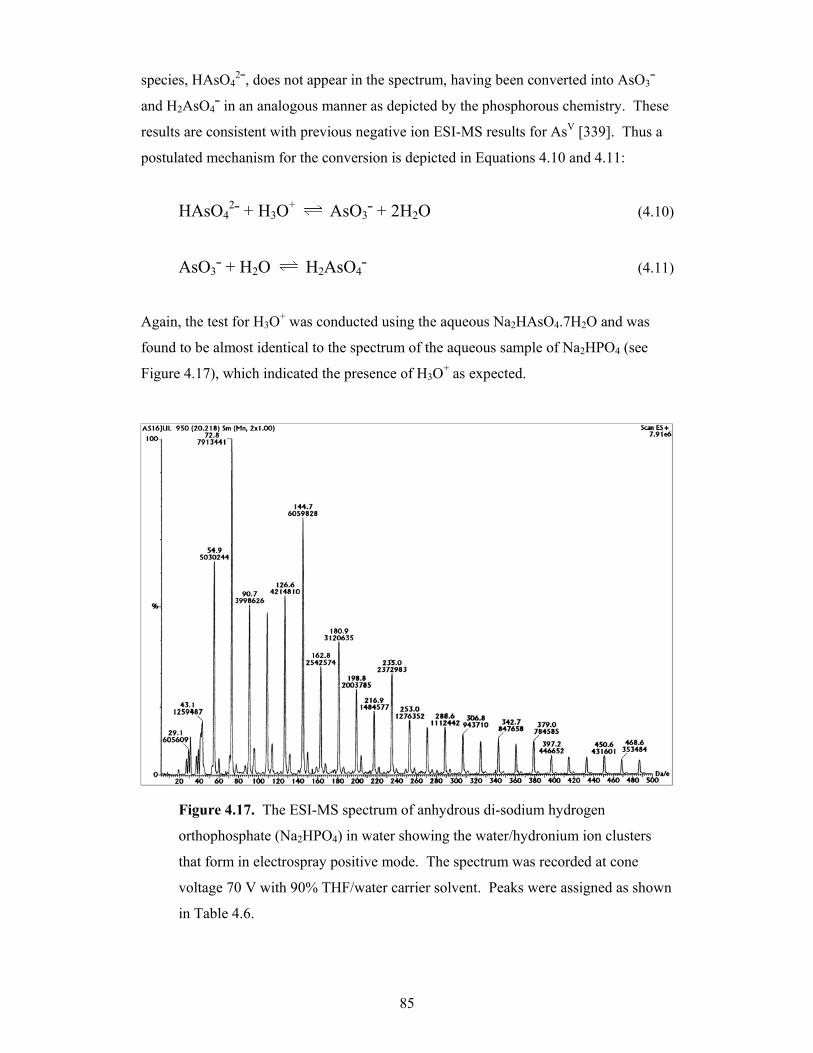
85
species, HAsO42¯, does not appear in the spectrum, having been converted into AsO3¯
and H2AsO4¯ in an analogous manner as depicted by the phosphorous chemistry. These
results are consistent with previous negative ion ESI-MS results for AsV [339]. Thus a
postulated mechanism for the conversion is depicted in Equations 4.10 and 4.11:
HAsO42¯ + H3O+ AsO3¯ + 2H2O (4.10)
AsO3¯ + H2O H2AsO4¯ (4.11)
Again, the test for H3O+ was conducted using the aqueous Na2HAsO4.7H2O and was
found to be almost identical to the spectrum of the aqueous sample of Na2HPO4 (see
Figure 4.17), which indicated the presence of H3O+ as expected.
Figure 4.17. The ESI-MS spectrum of anhydrous di-sodium hydrogen
orthophosphate (Na2HPO4) in water showing the water/hydronium ion clusters
that form in electrospray positive mode. The spectrum was recorded at cone
voltage 70 V with 90% THF/water carrier solvent. Peaks were assigned as shown
in Table 4.6.
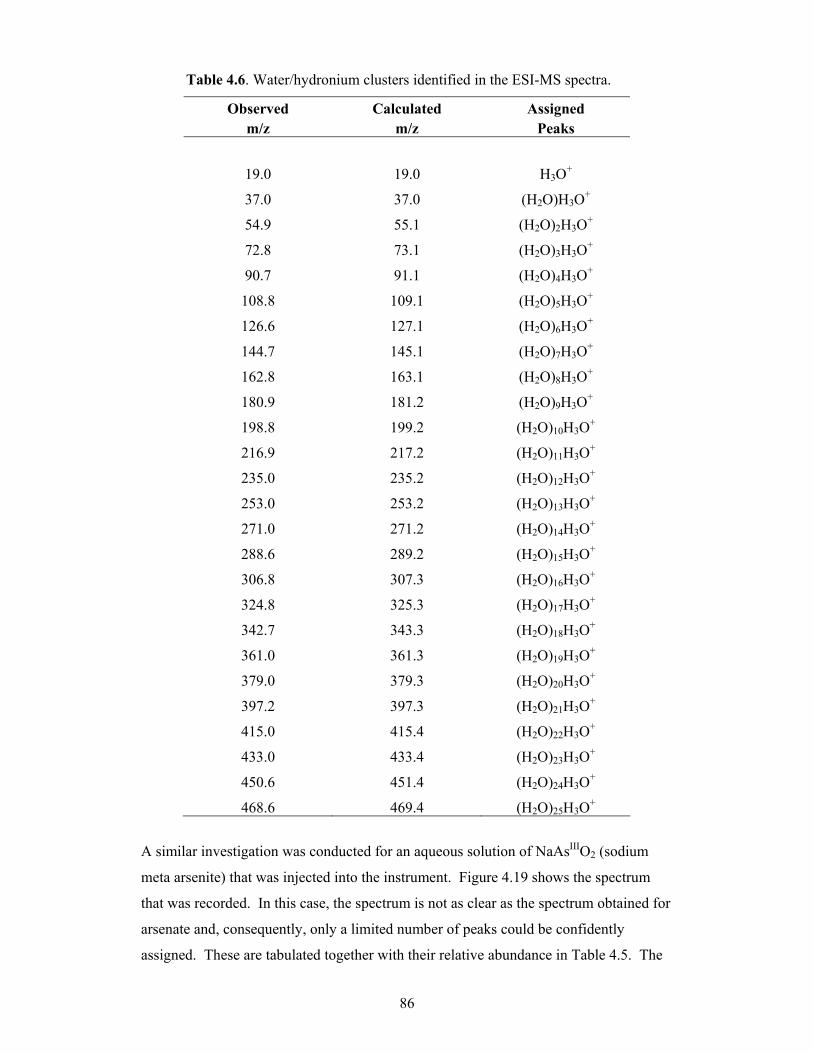
86
Table 4.6. Water/hydronium clusters identified in the ESI-MS spectra.
Observed Calculated Assigned m/z m/z Peaks
19.0 19.0 H3O+
37.0 37.0 (H2O)H3O+
54.9 55.1 (H2O)2H3O+
72.8 73.1 (H2O)3H3O+
90.7 91.1 (H2O)4H3O+
108.8 109.1 (H2O)5H3O+
126.6 127.1 (H2O)6H3O+
144.7 145.1 (H2O)7H3O+
162.8 163.1 (H2O)8H3O+
180.9 181.2 (H2O)9H3O+
198.8 199.2 (H2O)10H3O+
216.9 217.2 (H2O)11H3O+
235.0 235.2 (H2O)12H3O+
253.0 253.2 (H2O)13H3O+
271.0 271.2 (H2O)14H3O+
288.6 289.2 (H2O)15H3O+
306.8 307.3 (H2O)16H3O+
324.8 325.3 (H2O)17H3O+
342.7 343.3 (H2O)18H3O+
361.0 361.3 (H2O)19H3O+
379.0 379.3 (H2O)20H3O+
397.2 397.3 (H2O)21H3O+
415.0 415.4 (H2O)22H3O+
433.0 433.4 (H2O)23H3O+
450.6 451.4 (H2O)24H3O+
468.6 469.4 (H2O)25H3O+
A similar investigation was conducted for an aqueous solution of NaAsIIIO2 (sodium
meta arsenite) that was injected into the instrument. Figure 4.19 shows the spectrum
that was recorded. In this case, the spectrum is not as clear as the spectrum obtained for
arsenate and, consequently, only a limited number of peaks could be confidently
assigned. These are tabulated together with their relative abundance in Table 4.5. The
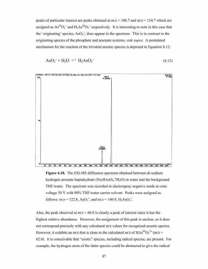
87
peaks of particular interest are peaks obtained at m/z = 106.7 and m/z = 124.7 which are
assigned as AsIIIO2¯ and H2AsIIIO3¯ respectively. It is interesting to note in this case that
the ‘originating’ species, AsO2¯, does appear in the spectrum. This is in contrast to the
originating species of the phosphate and arsenate systems, vide supra. A postulated
mechanism for the reaction of the trivalent arsenic species is depicted in Equation 4.12:
AsO2¯ + H2O H2AsO3¯ (4.12)
Figure 4.18. The ESI-MS difference spectrum obtained between di-sodium
hydrogen arsenate heptahydrate (Na2HAsO4.7H2O) in water and the background
THF/water. The spectrum was recorded in electrospray negative mode at cone
voltage 30 V with 90% THF/water carrier solvent. Peaks were assigned as
follows: m/z = 122.8, AsO3¯; and m/z = 140.9, H2AsO4¯.
Also, the peak observed at m/z = 60.8 is clearly a peak of interest since it has the
highest relative abundance. However, the assignment of this peak is unclear, as it does
not correspond precisely with any calculated m/z values for recognized arsenic species.
However, it exhibits an m/z that is close to the calculated m/z of HAsIIIO32¯ (m/z =
62.0). It is conceivable that “exotic” species, including radical species, are present. For
example, the hydrogen atom of the latter species could be abstracted to give the radical
88
dianion (AsIIIO3˙)2¯ (for which m/z = 61.5 – and is closer to the experimental value).
However, it is beyond the scope of this thesis to pursue such species further.
Other peaks assigned at m/z = 45.9 (AsVO43¯), 122.6 (AsVO3¯), 124.7 (H2AsVO3¯) and
m/z = 140.5 (H2AsVO4¯) appear to provide evidence of the formation of oxidative
contaminants or products. Such species may have been produced in the bottle
containing the solid sample or in the aqueous stock solution. The former situation
would appear to be more likely considering that AsIII is susceptible to aerobic oxidation.
However, AsIII may persist in aerated water due to slow oxidation kinetics [340]. It is
also possible that oxidation of AsIII could have taken place on entering the ESI-MS
ionisation chamber. However, a low cone voltage was used (i.e. 30 V) to reduce the
likelihood of such oxidation. It has been demonstrated that lower cone voltages (i.e. ≤
30 V) tend to preserve dissolved-phase speciation [341]. In light of the above findings,
it is possible that ESI-MS may prove to be a suitable method to routinely assay the
“oxidative purity” of such samples.
4.4.2 Computer Modelling of Phosphate, Arsenate and Arsenite
All species detected by the ESI-MS were modelled by high-level density functional
calculations (see Section 3.4). The primary imperative is to provide supporting
evidence for the reaction mechanisms proposed in Section 4.4.1 in terms of the relative
energies of the species involved and the calculated reaction energies. However, in the
course of these calculations, a considerable amount of further information on these
species has been obtained and documented in this thesis (see Section 4.4.2.2).
4.4.2.1 Energies of Species and Reaction Energies
The calculated energies for each of the species detected in the ESI-MS experiments are
given in Table 4.7. The reaction energies were calculated in each case for the
phosphate, arsenate and arsenite systems by subtracting the reactant energies from the
product energies.
In the case of the phosphate system, the suggested mechanism consists of the two
processes that are represented by Equations 4.8 and 4.9. The reaction energy for each of
these equations has been calculated as indicated below:
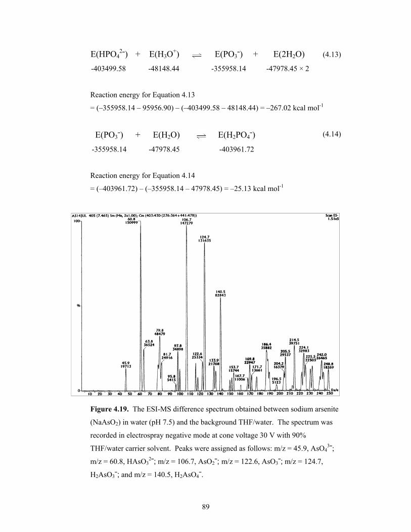
89
E(HPO42¯) + E(H3O+) E(PO3¯) + E(2H2O) (4.13)
-403499.58 -48148.44 -355958.14 -47978.45 × 2
Reaction energy for Equation 4.13
= (–355958.14 – 95956.90) – (–403499.58 – 48148.44) = –267.02 kcal mol-1
E(PO3¯) + E(H2O) E(H2PO4¯) (4.14)
-355958.14 -47978.45 -403961.72
Reaction energy for Equation 4.14
= (–403961.72) – (–355958.14 – 47978.45) = –25.13 kcal mol-1
Figure 4.19. The ESI-MS difference spectrum obtained between sodium arsenite
(NaAsO2) in water (pH 7.5) and the background THF/water. The spectrum was
recorded in electrospray negative mode at cone voltage 30 V with 90%
THF/water carrier solvent. Peaks were assigned as follows: m/z = 45.9, AsO43¯;
m/z = 60.8, HAsO32¯; m/z = 106.7, AsO2¯; m/z = 122.6, AsO3¯; m/z = 124.7,
H2AsO3¯; and m/z = 140.5, H2AsO4¯.
90
In Equation 4.13, the negative reaction energy, –267.02 kcal mol-1, indicates that the
reaction favours the right hand side, i.e. the formation of the products PO3¯ and H2O.
The reaction proceeds further as shown in Equation 4.14 which, similarly, has the
negative reaction energy, –25.13 kcal mol-1, favouring the formation of the product
H2PO4¯. These results support the postulated mechanism for the formation of the
monomeric phosphate species detected in the ESI-MS spectrum.
Using the phosphate system as a benchmark, analogous reaction energy calculations
were carried out for the arsenate system. Thus using analogous calculations to those
depicted in Equations 4.10 and 4.11, the calculated reaction energies for the arsenate
system are –265.10 kcal mol-1 and –22.30 kcal mol-1 respectively. These reaction
energies support the postulated reaction mechanism for the formation of the arsenic
species detected in the ESI-MS spectrum. The magnitudes are also very similar to those
for the phosphorous system. It is also of interest to note that when the relative energies
of the phosphorus and arsenic species are compared it is evident that both AsO3¯ and
H2AsO4¯ are more stable than their phosphorous analogues, PO3¯ and H2PO4¯.
Similar reaction energy calculations were carried out for the arsenite system. The
postulated mechanism is shown in Equation 4.12. Here, the calculated reaction energy
is –70.84 kcal mol-1. Similar to the other systems already discussed, this reaction
energy indicates that the equation favours the formation of the product H2AsO3¯, hence
supporting the postulated mechanism.
Estimates for the equilibrium constants for reactions 4.3, 4.5 and 4.6 may be obtained in
each case by taking the ratio of the relative energies of product to reactant. For
example, a ratio for the energy of the two monomeric phosphate species detected in the
ESI-MS was calculated by dividing the energy of H2PO4¯ by the energy of PO3¯ as
shown in Equation 4.15. The ratio gives a constant (K) equal to 1.13 indicating that the
H2PO4¯ species is slightly favoured over the PO3¯ species within the ESI-MS
environment.
E(H2PO4¯) -403961.72 E(PO3¯)
= -355958.14
= 1.13 (4.15)
91
Similarly, an energy ratio calculation was made for the two arsenate species detected in
the ESI-MS (see Equation 4.16). In this case a value of K = 1.03 suggests that the
H2AsO4¯ species is slightly favored over the AsO3¯ species.
E(H2AsO4¯) -1592719.36 E(AsO3¯)
= -1544718.61
= 1.03 (4.16)
The above estimates for the relative equilibrium constants (1.13 compared to 1.03 for
phosphorous and arsenic respectively) reflect the relative abundances of the phosphorus
species (30.3/5.9 = 5.14) compared to the arsenic species (54.9/16.8 = 1.13), Table 4.5.
It must be born in mind, however, that this comparison is complicated by the presence
of polymeric species in the case of phosphorus, presumably derived from PO3¯.
4.4.2.2 Geometries
As part of the species energy and reaction energy calculations a number of geometries
and other molecular information emerged for each of the phosphorus and arsenic
species detected in the ESI-MS. These are clearly of interest and are presented, and
compared to reported crystallographic data, in Table 4.7.
A feature of the computed PO3¯ species is that it forms a trigonal planar structure that is
perfectly symmetrical with all bond angles at 120° and all bond lengths at 1.503 Å.
This might be, naively, unexpected - when one considers the valence bond
representation where PO3¯ is represented with two double P=O bonds and one single P-
O bond, see Chart 4.1. Therefore, the computed structure suggests that PO3¯ is a
resonance structure with delocalised electrons, where the double and single bonds
effectively average out. Thus the three computed P-O (hybrid) bond lengths of 1.503 Å
are very close to the computed P=O and P-O¯ bond lengths (both 1.500 Å) of the trans
isomer of the H2PO4¯ species (that is also a monoanion4) and are essentially an average
(1.500 Å) of the computed P=O and P-O¯ bond lengths of 1.513 Å and 1.491 Å
respectively for the cis isomer of H2PO4¯, Table 4.7. The possibility of cis and trans
isomers for the latter species and the implications of this are discussed in more detail
4 It is found that, for phosphorus and arsenic species, the P(As) - O bond lengths increase with an increase in charge. This is discussed further in the text.
92
later. This resonance is also reflected in the electrostatic potential energy map, Chart
4.1, as discussed later.
The AsO3¯ species is entirely analogous to PO3¯ in terms of its perfect trigonal
symmetry and delocalised electrons, Chart 4.2. Thus the three bond lengths in AsO3¯
are identical at 1.655 Å. They are also considerably longer than the corresponding bond
lengths in PO3¯. Furthermore, the three As-O (hybrid) bond lengths of 1.655 Å are
almost identical to the As=O and As-O¯ bond lengths (both 1.654 Å) for the trans
isomer of the H2AsO4¯ species and are essentially an average (1.655 Å) of the computed
P=O and P-O¯ bond lengths of 1.644 Å and 1.665 Å respectively for the cis isomer of
H2AsO4¯, Table 4.7.
The computed geometries for the species HXO42¯ (X = P, As) show distorted tetrahedral
geometries with O-X-O angles ranging from 102.19 – 116.13° and 102.01 – 116.60°
respectively, Table 4.7. These compare favourably with the crystallographic data [342]
for these species of 102.7 – 114.2° and 102.7 – 113.7° respectively. The comparative
X-OH, X=O and the X-O¯ bond lengths in the computed species tend to be longer than
the crystallographic values. This is particularly pronounced for X-OH. This is perhaps,
not unexpected, given that the computed values are in vacuo and the crystallographic
geometries are subject to crystal packing forces such as intermolecular hydrogen
bonding. This argument is also true with respect to angles. In this regard, the computed
structures for HXO42¯ have a plane of symmetry that is broken in the crystal structures
as reflected in the values for angles O=X-O¯ and O¯-X-OH in Table 4.7. For example,
the computed values for the two O=P-O¯ angles in HPO42¯ are both identically 116.13°,
whereas the corresponding angles in the crystal structure are 112.2° and 114.2°.
The computed geometries for the species H2XO4¯ (X = P, As) also show distorted
tetrahedral geometries, with O-X-O angles, including both cis and trans isomers,
ranging from 100.91 – 126.25° and 100.00 – 128.67° respectively, Table 4.7. The upper
values represent considerable distortion of the O=X-O¯ angles in all cases and reflect
the presence of strong intramolecular hydrogen bonds in the computed structures, as
indicated in Chart 4.3. Notably, in the crystal structure of H2XO42¯ the range of O-X-O
angles is 106.5 – 115.5° [342] and 105.1 – 116.5° [343] respectively. The relief in
distortion is probably due to the presence of competing intermolecular hydrogen
bonding in the crystal structure. The computed X-OH, X=O and the X-O¯ bond lengths

93
in the monoanions are shorter than in the previous HXO42¯ dianions. This bond length
dependency on formal charge has also been observed experimentally upon going from
the dianion to the neutral H3PO4 [342]. For this reason the bond lengths and angles for
the latter species have also been included in Table 4.7. The computed P-OH bond
lengths are longer than in the crystal structure. Again, this is attributed to the presence
of crystal packing forces, particularly intermolecular hydrogen bonding, in the latter
case.
The two arsenite species, AsIIIO2¯ and H2AsIIIO3¯, detected in the ESI-MS, exhibit
interesting computed geometries as depicted in Chart 4.4. The AsO2¯ species forms a
linear structure with equivalent As-O bond lengths of 1.721 Å. This appears to be
elongated with respect to both the As=O and As-O¯ bonds in H2AsVO4¯. However, it
should be realized that arsenic species in the +III oxidation state are intuitively expected
to exhibit a contraction of bond lengths with increasing oxidation state. Like PO3¯ and
AsO3¯, vide supra, AsO2¯ displays a delocalised electron configuration where the double
and single bonds are effectively averaged out.
The H2AsO3¯ species forms an interesting pyramidal shape, Chart 4.4, analogous to the
shape of H3PO3, that is proposed to be in equilibrium with its tetrahedral tautomer [287],
i.e.:
In the latter structure, a proton has transferred from an oxygen atom to the phosphorus
atom. Here, the tetrahedral structure is computed to be 11.11 kcal mol-1 more stable
than the pyramidal. This is consistent with the tetrahedral structure being reported [286-
287] as the favoured equilibrium species. In this regard the pyramidal tautomer of the
arsenic species is computed to be 27.68 kcal mol-1 more stable than the tetrahedral,
Table 4.7. Therefore, whereas the tetrahedral species is the more stable for phosphorus,
the pyramidal is the more stable for arsenic. It is clear from the HOMO representation
of the pyramidal structure of H2AsO3¯, Chart 4.4, that a lone pair is available to receive
a proton from one of the hydroxyl groups. This is also true for phosphorus (not
represented here).
94
It should be pointed out that, for H2AsO3¯, a structure that is intermediate in energy
between the pyramidal and the tetrahedral may also be satisfactorily computed, Table
4.7. This has an unusual T-shaped structure with the O-H groups cis to one another,
Chart 4.5. The trans configuration is also possible but is higher in energy than the other
three isomers. For the phosphorous analogues, only the trans-T-shaped structure can be
computed and this is considerably higher in energy than the pyramidal and the
tetrahedral (-35668.5 > -356705.2 > -356716.3 kcal mol-1). The cis configuration tends
to revert to the pyramidal upon refinement and is therefore postulated not to exist.
The bond lengths and angles for the four arsenic isomers of H2AsO3¯ (pyramidal, cis-T-
shaped, tetrahedral and trans-T-shaped) are given Table 4.7. The respective As-OH
bond lengths are 1.901, 2.022, 1.853 and 2.019/2.053 Å. Notably the pyramidal and
tetrahedral bond lengths are shorter than those in the cis/trans isomers suggesting that
flattening out the structures brings about an elongation of this type of bond. The
respective As-O bond lengths are 1.683, 1.664, 1.667 and 1.651 Å and, as observed
previously, are shorter that the As-OH bonds. The bond lengths of H2AsIIIO3¯ are also
observed to be elongated with respect to similar types of bonds in the monoanionic
H2AsVO4¯ species. This is consistent with the notion that, for the same type of bond, a
lower oxidation state results in bond lengthening. The As=O bond length in the
tetrahedral isomer is 1.657 Å. This is consistent with corresponding bond lengths in
other arsenic species. The As-H bond length in the tetrahedral isomer is 1.536 Å. From
the data in Table 4.7 it is possible to estimate that the average bond lengthening in
vacuo compared to the crystal structure data (where crystal packing forces are in effect)
is approximately 3.5%. This would result in a “corrected” As-H distance of 1.48 Å that
is comparable to the sum of the respective covalent radii, 1.49 Å [344]. Notably, in the
H3PO3 tetrahedral analogue this hydrogen is not considered to be available and the
species is considered to be dibasic only [286-287]. This is also expected to be the case
for arsenic. Indeed, the LUMO representation of the tetrahedral H2AsO3¯ shows this
hydrogen to be non-acidic.
The O-As-OH bond angles for the pyramidal, cis-T-shape, tetrahedral and trans-T-
shape isomers are 100.23°, 94.04°, 103.81° and 94.71/94.42° respectively with the T-
shaped isomers exhibiting smaller bond angles as a result of their flattened structure,
vide supra. The OH-As-OH bond angles for the pyramidal, cis-T-shape and trans-T-
95
shape isomers are 98.59°, 171.93° and 170.87° with the T-shaped structures showing
larger bond angles compared to the pyramidal isomer. The O=As-O¯ and O=As-OH
bond angles in the tetrahedral isomer are observed to be slightly less distorted with
respect to similar types of bonds in the monoanionic H2AsVO4¯ species. Attempts to
find crystal structure information for the arsenite species proved to be unsuccessful.
This has also been noted by others [345] for the H3AsO3 species. However, crystal
structure information was reported for an AsO2OH fragment present in a
(C3H12N2)2[H2As6Mo4O22].2H2O [345] structure. In that particular fragment species the
reported crystal structure distance for an As-O bond is 1.801 Å. This is longer than the
modelled H2AsO3¯ species but would appear to be consistent with the expected
elongation of dianion species compared to monoanion and neutral species, vide supra,
see Table 4.7.
4.4.2.3 Electrostatic potential energy calculations
The electrostatic potential energy maps were also calculated for each of the phosphorus
and arsenic species, along with calculated energies for the highest occupied molecular
orbital (EHOMO) and lowest unoccupied molecular orbital (ELUMO). Both qualitative and
graphical representations are provided. The EHOMO and ELUMO values are given in Table
4.7 and the electrostatic potential energy maps along with the HOMO and LUMO
graphics are presented in Charts 4.1, 4.2, 4.4 and 4.5.
The EHOMO is of particular interest because it gives an indication of the reactivity of the
species of interest, with higher EHOMO values indicating more reactivity [346]. It has
been reported that the value of EHOMO could be a first approximation to the
nucleophilicity of the compound [346-347]. Generally speaking, the HOMO of these
phosphorus and arsenic species are likely to form bonds with the LUMO of other
species that might be present (i.e. possibly in soil or water). The calculated LUMO
energy of the phosphorus and arsenic species also provide useful information because
any further electrons that enter the system will be accommodated in the LUMO, the
energetically most accessible unfilled molecular orbital. Hence, the LUMO may be
thought of as demarking the location of positive charge in a molecule [290]. It has also
been suggested that the ELUMO could also be a first approximation to the electrophilicity
of the compound [346-347].

96
Table 4.7. Geometries and further information for phosphorus and arsenic species.
PO3¯ HPO42¯ HPO4
2¯ trans H2PO4¯ cis H2PO4¯ H2PO4¯ H3PO4 Modelled Modelled Crystal Modelled Modelled Crystal Crystal Structure [342] Structure [342] Structure [342] Bond Angle / ° O=X-O¯ 120.00 116.13 112.2, 114.2 126.25 125.93 115.5 O=X-OH 102.19 102.7 106.80, 106.66 107.52 110.4, 108.4 112.0, 113.2, 113.0 O¯-X-OH 102.80 106.9, 107.5 106.65, 106.80 105.95 107.2 , 108.5 OH-X-OH 100.91 101.35 106.5 105.6, 107.3, 104.9 X-O-H 102.31 106.72 106.25 O=X=O 120.00 O¯-X-O¯ 113.89 112.5 H-X-O¯ H-X-OH Bond Length / Å X-OH 1.783 1.618 1.680 1.679 1.572, 1.556 1.545, 1.548, 1.545 O-H 0.962 0.963 0.962 X=O 1.503 1.537 1.535 1.500 1.491 1.504 1.496 X-O¯ 1.503 1.548 1.522, 1.529 1.500 1.513 1.515 X-H O¯ - - H (H bonding) Energy / kcal mol-1 -355958.14 -403499.58 -403961.72 -403960.78 ∆E(Ecis - Etrans) / kcal mol-1 0.94 CPKVOLUME / Å3 49.02 61.15 63.06 CPKAREA / Å2 72.26 88.99 91.48 WEIGHT / g mol-1 78.971 95.978 96.986 EHOMO / kcal mol-1 -51.44 91.46 -56.60 ELUMO / kcal mol-1 76.70 175.40 78.48 DIPOLE / Debye 0 5.85 5.69
X denotes the element phosphorus or arsenic for the respective phosphorus or arsenic species
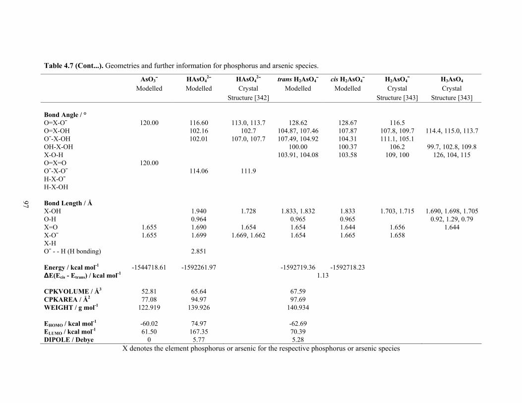
97
Table 4.7 (Cont...). Geometries and further information for phosphorus and arsenic species.
AsO3¯ HAsO42¯ HAsO4
2¯ trans H2AsO4¯ cis H2AsO4¯ H2AsO4¯ H3AsO4 Modelled Modelled Crystal Modelled Modelled Crystal Crystal Structure [342] Structure [343] Structure [343] Bond Angle / ° O=X-O¯ 120.00 116.60 113.0, 113.7 128.62 128.67 116.5 O=X-OH 102.16 102.7 104.87, 107.46 107.87 107.8, 109.7 114.4, 115.0, 113.7O¯-X-OH 102.01 107.0, 107.7 107.49, 104.92 104.31 111.1, 105.1 OH-X-OH 100.00 100.37 106.2 99.7, 102.8, 109.8 X-O-H 103.91, 104.08 103.58 109, 100 126, 104, 115 O=X=O 120.00 O¯-X-O¯ 114.06 111.9 H-X-O¯ H-X-OH Bond Length / Å X-OH 1.940 1.728 1.833, 1.832 1.833 1.703, 1.715 1.690, 1.698, 1.705O-H 0.964 0.965 0.965 0.92, 1.29, 0.79 X=O 1.655 1.690 1.654 1.654 1.644 1.656 1.644 X-O¯ 1.655 1.699 1.669, 1.662 1.654 1.665 1.658 X-H O¯ - - H (H bonding) 2.851 Energy / kcal mol-1 -1544718.61 -1592261.97 -1592719.36 -1592718.23 ∆E(Ecis - Etrans) / kcal mol-1 1.13 CPKVOLUME / Å3 52.81 65.64 67.59 CPKAREA / Å2 77.08 94.97 97.69 WEIGHT / g mol-1 122.919 139.926 140.934 EHOMO / kcal mol-1 -60.02 74.97 -62.69 ELUMO / kcal mol-1 61.50 167.35 70.39 DIPOLE / Debye 0 5.77 5.28
X denotes the element phosphorus or arsenic for the respective phosphorus or arsenic species
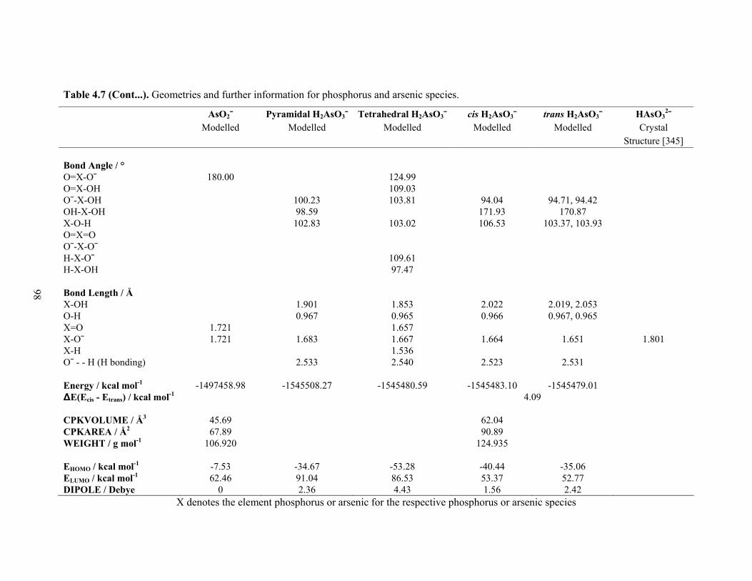
98
Table 4.7 (Cont...). Geometries and further information for phosphorus and arsenic species.
AsO2¯ Pyramidal H2AsO3¯ Tetrahedral H2AsO3¯ cis H2AsO3¯ trans H2AsO3¯ HAsO32¯
Modelled Modelled Modelled Modelled Modelled Crystal Structure [345] Bond Angle / ° O=X-O¯ 180.00 124.99 O=X-OH 109.03 O¯-X-OH 100.23 103.81 94.04 94.71, 94.42 OH-X-OH 98.59 171.93 170.87 X-O-H 102.83 103.02 106.53 103.37, 103.93 O=X=O O¯-X-O¯ H-X-O¯ 109.61 H-X-OH 97.47 Bond Length / Å X-OH 1.901 1.853 2.022 2.019, 2.053 O-H 0.967 0.965 0.966 0.967, 0.965 X=O 1.721 1.657 X-O¯ 1.721 1.683 1.667 1.664 1.651 1.801 X-H 1.536 O¯ - - H (H bonding) 2.533 2.540 2.523 2.531 Energy / kcal mol-1 -1497458.98 -1545508.27 -1545480.59 -1545483.10 -1545479.01 ∆E(Ecis - Etrans) / kcal mol-1 4.09 CPKVOLUME / Å3 45.69 62.04 CPKAREA / Å2 67.89 90.89 WEIGHT / g mol-1 106.920 124.935 EHOMO / kcal mol-1 -7.53 -34.67 -53.28 -40.44 -35.06 ELUMO / kcal mol-1 62.46 91.04 86.53 53.37 52.77 DIPOLE / Debye 0 2.36 4.43 1.56 2.42
X denotes the element phosphorus or arsenic for the respective phosphorus or arsenic species
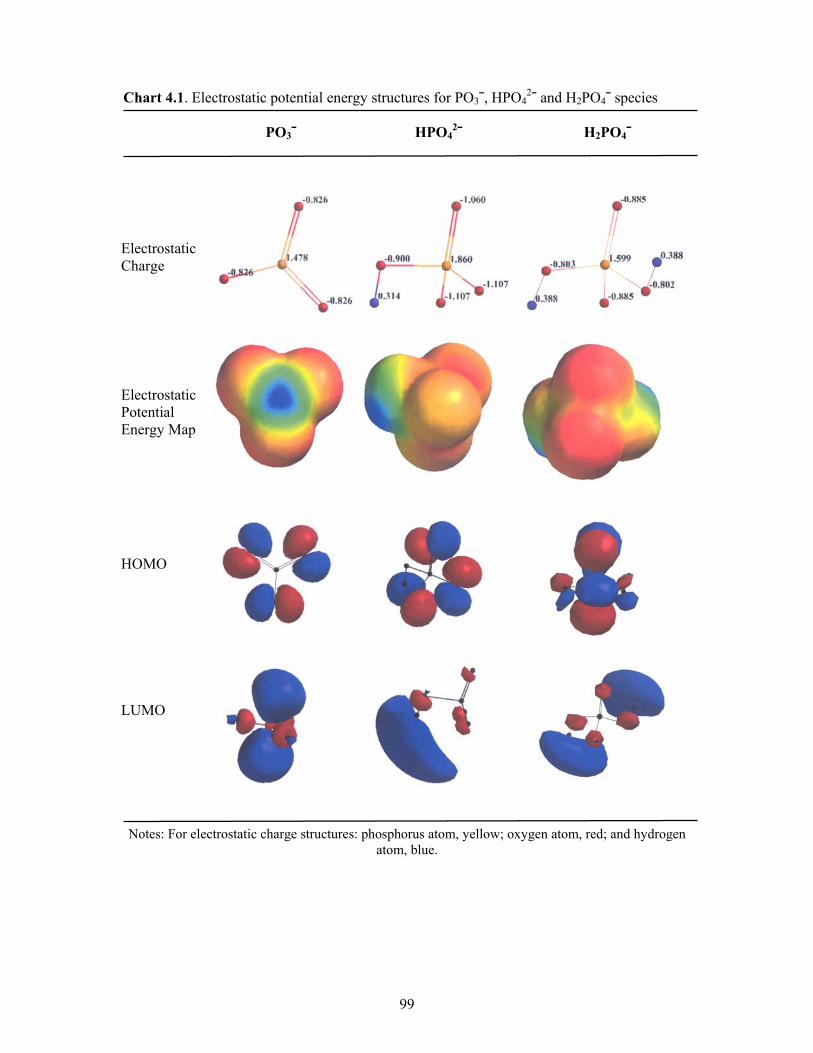
99
Chart 4.1. Electrostatic potential energy structures for PO3¯, HPO42¯ and H2PO4¯ species
PO3¯ HPO4
2¯ H2PO4¯
Notes: For electrostatic charge structures: phosphorus atom, yellow; oxygen atom, red; and hydrogen
atom, blue.
Electrostatic Potential Energy Map
Electrostatic Charge
HOMO
LUMO
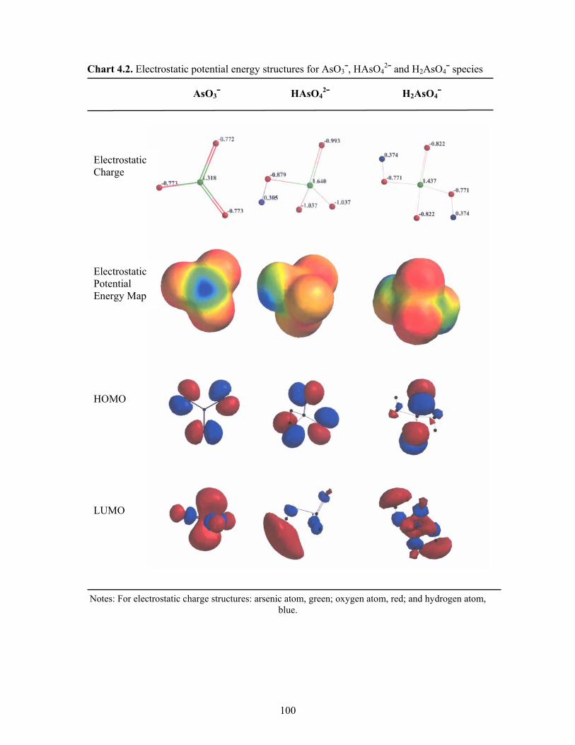
100
Chart 4.2. Electrostatic potential energy structures for AsO3¯, HAsO42¯ and H2AsO4¯ species
AsO3¯ HAsO4
2¯ H2AsO4¯
Notes: For electrostatic charge structures: arsenic atom, green; oxygen atom, red; and hydrogen atom,
blue.
Electrostatic Potential Energy Map
Electrostatic Charge
HOMO
LUMO
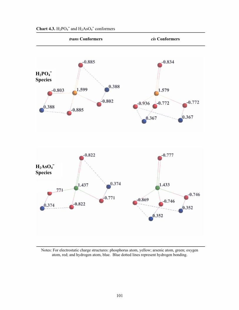
101
Chart 4.3. H2PO4¯ and H2AsO4¯ conformers trans Conformers cis Conformers
Notes: For electrostatic charge structures: phosphorus atom, yellow; arsenic atom, green; oxygen atom, red; and hydrogen atom, blue. Blue dotted lines represent hydrogen bonding.
H2PO4¯
Species
H2AsO4¯
Species
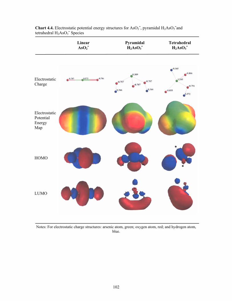
102
Chart 4.4. Electrostatic potential energy structures for AsO2¯, pyramidal H2AsO3¯and tetrahedral H2AsO3¯ Species Linear Pyramidal Tetrahedral AsO2¯ H2AsO3¯ H2AsO3¯
Notes: For electrostatic charge structures: arsenic atom, green; oxygen atom, red; and hydrogen atom,
blue.
Electrostatic Potential Energy Map
Electrostatic Charge
HOMO
LUMO
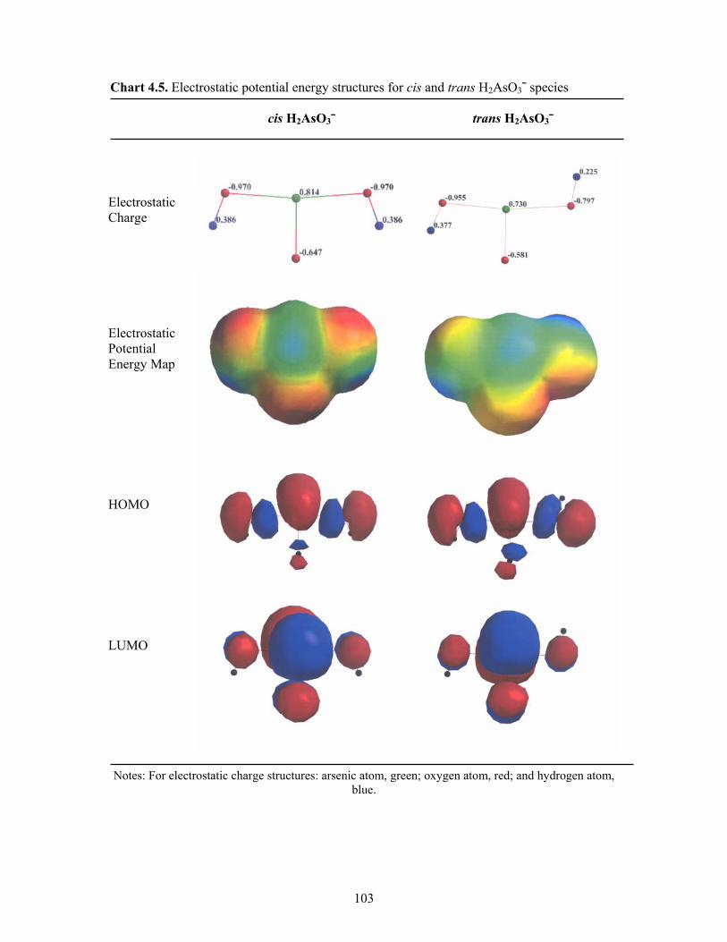
103
Chart 4.5. Electrostatic potential energy structures for cis and trans H2AsO3¯ species cis H2AsO3¯ trans H2AsO3¯
Notes: For electrostatic charge structures: arsenic atom, green; oxygen atom, red; and hydrogen atom,
blue.
Electrostatic Potential Energy Map
Electrostatic Charge
HOMO
LUMO

104
-80.00
-60.00
-40.00
-20.00
0.00
20.00
40.00
60.00
80.00
100.00
Species
EH
OM
O /
kcal
mol
-1
MostNucleophilic
LeastNucleophilic
PO3¯ HPO42¯ H2PO4¯ AsO3¯ HAsO4
2¯ H2AsO4¯ AsO2¯ H2AsO3¯
Figure 4.20. Relative computed EHOMO values.
0.00
20.00
40.00
60.00
80.00
100.00
120.00
140.00
160.00
180.00
200.00
Species
EL
UM
O /
kcal
mol
-1
LeastElectrophilic
MostElectrophilic
PO3¯ HPO42¯ H2PO4¯ AsO3¯ HAsO4
2¯ H2AsO4¯ AsO2¯ H2AsO3¯
Figure 4.21. Relative computed ELUOMO values.
The order of highest to lowest EHOMO for the phosphorus and arsenic species
investigated are: HPO42¯ > HAsO4
2¯ > AsO2¯ > H2AsO3¯ >PO3¯ > H2PO4¯ > AsO3¯ >
H2AsO4¯ which indicates that the HPO42¯ and HAsO4
2¯ are the most reactive phosphorus
and arsenic species respectively (see Table 4.7). This is consistent with the reactions

105
that are observed in the ESI-MS. The relative EHOMO values for all species detected by
ESI-MS are shown in Figure 4.20. Similarly, the relative ELUMO values are shown in
Figure 4.21.
The electrostatic potential energy maps for the PO3¯/HPO42¯/H2PO4¯ species, the
AsO3¯/HAsO42¯/H2AsO4¯ species, the AsO2¯/pyramidal H2AsO3¯/ tetrahedral H2AsO3¯
and the cis and trans H2AsO3¯ species respectively are presented in Charts 4.1, 4.2, 4.4
and 4.5. These maps give the electrostatic potential at locations on a particular surface,
most commonly a surface of electron density corresponding to overall molecular size
[290]. Colours are used in the electrostatic potential energy maps to designate values of
the potential. Colours close to red represent large negative values of potential, while
colours close to blue represent large positive values. Orange, yellow and green
represent intermediate values of potential. The electrostatic potential energy maps serve
to quickly characterise various regions in a molecule as electron rich or electron poor, or
neither rich nor poor [290]. In the planar PO3¯ and AsO3¯ species the areas near the
surface oxygen atoms are shown in red indicating large negative potential values
associated with electron rich areas. Whereas, the central phosphorus or arsenic atoms
are shown in blue which represent a positive potential value associated with an electron
poor area. The electrostatic potential energy maps for PO3¯ and AsO3¯ species are of
particular interest because they clearly illustrate the delocalised electron configuration.
As expected, the tetrahedral HXO42¯ and H2XO4¯ species display negative potential
values (i.e. electron rich areas) on the oxygen atoms and exhibit positive potential
values (i.e. electron poor areas) on the X and hydrogen atoms. In the H2XO4¯ species, it
is of interest to compare the effect of cis/trans isomerism on the electrostatics, Chart
4.3. For both phosphorus and arsenic trans isomers the intramolecular H-bonding
arrangement results in an effective delocalisation of electrons over the O=X-O¯ bond.
This is reflected in the fact that the X=O and the X-O¯ bond lengths are identical in
these isomers, Table 4.7. This is not the case for the cis isomers. This is consistent
with the trans isomers being more stable than the cis by approx. 1 kcal mol-1. This is an
example of where an alternative intramolecular hydrogen bonding arrangement within a
molecule can result in additional stabilization.
The AsO2¯ and H2AsO3¯ species exhibit interesting structures and electrostatic potential
energy maps. In the case of AsO2¯ the structure has a linear shape with a delocalised
106
electron configuration that leads to electron rich areas located at either end of the
molecule and an electron poor area in the middle. The isomeric H2AsO3¯ species
display pyramidal, tetrahedral and unusual planar T-shape structures that, as expected,
exhibit electron rich areas on the oxygen atoms and electron poor areas on the hydrogen
atoms and the central arsenic atoms.
4.4.3 Extraction of Arsenite from Soil
The quantification of arsenite in soil was performed using a chloroform extraction
technique [32] that is described in Section 3.4.3. The technique was first used to
quantify the purity of the arsenite sample utilized in experimental work (see Section
4.4.3.1) and then used to determine the amount of AsIII sorbed onto soil at different pH
(see Section 4.4.3.2).
4.4.3.1 Standardisation of Arsenite Sample
An examination of the ESI-MS spectrum (Section 4.4.1.2) of an aqueous solution of the
arsenite “standard” that was made up, suggested the presence of oxidative impurities.
These were, originally, thought to have formed either in the ESI-MS ionisation chamber
or in the aqueous stock solution after being made up. However, both of these ideas
were subsequently dismissed for the reasons discussed in Section 4.4.1.2. It was
concluded that the presence of these impurities originated with the supplied arsenite
salt. In order to quantify the amount of AsIII present and to gain more insight into the
nature of such purported oxidative processes, the chloroform extraction technique was
implemented as follows:
Three different aqueous stock solutions containing the following arsenic species: (i)
AsIII as NaAsO2; (ii) AsV as Na2AsO4.7H2O; and (iii) 50% v/v mixture of AsIII and AsV
stock solutions were prepared. The AsTot was determined in each case. The measured
AsIII and AsTot were compared to calculated AsIII and AsTot concentrations as shown in
Table 4.8. The results indicate that the aqueous stock solution of NaAsO2 contained
65.9 mg L-1 as AsIII and 76.7 mg L-1 as AsTot. It is noted, in these results, that the
concentration of AsIII is approximately 14% lower than the AsTot concentration. This is
consistent with the likelihood of oxidative impurities suggested by the ESI-MS. The
calculated concentration, of both AsIII and AsTot, assuming a pure aqueous stock
107
solution of NaAsO2 is 83.6 mg L-1. The fact that this is higher than the 76.7 mg L-1
measured for AsTot reflects the presence of such (oxidized) species in the salt. The
identity of such possible contaminants can be deduced from the ESI-MS as given in
Table 4.5. Such contaminants would be expected to be of a higher molecular weight
(MW) than the NaAsO2 and this would result in a lower value of the measured AsTot –
as observed. The following calculations have been made to support the theory that the
oxidative impurities have a higher molecular weight:
The concentration of AsIII in the first aqueous stock solution was determined to be
0.0659 g L-1 (Section 4.4.3.1, Table 4.8) which means that the required mass of pure
NaAsO2 to give such an answer can be calculated as follows:
Mass(NaAsO2) = 0.0659 g AsIII × [MW(NaAsO2)/MW(As)]
= 0.1143 g as NaAsO2 (4.17)
However, the mass of NaAsO2 actually added to the stock solution was 0.1450 g, so the
mass of the oxidative impurities can be calculated by subtracting the amount calculated
in Equation 4.17 from the actual mass added:
Mass of oxidative impurity = 0.1450 – 0.1143 = 0.0307 g (4.18)
The effective molecular weight of the oxidative impurities can be calculated by using
the concentration difference between the measured AsTot and AsIII (i.e. 0.0108 g L-1 -
values shown in Table 4.8) as follows:
MW(Oxidative impurities) = MW(As) × 0.0307 g / 0.0108 g = 213.2 g mol-1 (4.19)
Thus, it can be seen from Equation 4.19 that the effective molecular weight of the
oxidative impurities is in the vicinity of 213.2 g mol-1 that may correspond to the
Na3AsO4 species with a molecular weight of 207.89 g mol-1. This is in good agreement
with the ESI-MS results that suggests that the dominant oxidative species present is the
AsO43¯ species.
The chloroform extraction method results for the aqueous Na2AsO4.7H2O solution show
virtually no AsIII is present. The AsTot in this case is 55.1 mg L-1. The calculated

108
concentrations for AsIII and AsTot of 0 mg L-1 and 54.3 mg L-1 respectively, are therefore
consistent with the experimental values. An estimation of the error associated with the
data presented in Table 4.8 has been calculated using the 95% confidence limit (i.e.
t 0.05,6 = 1.943) of the arithmetic average concentration based on experimental data used
in Section 4.2.1 (see Table 4.2) that are based on seven replicates. The maximum error
calculated was ± 0.2 mg L-1 without dilution or ± 2 mg L-1 with dilution.
The 50% v/v mixture of AsIII and AsV stock solution also indicated consistent results
compared to the NaAsO2 solution which also exhibited lower than expected AsIII and
AsTot concentrations. The results for the aqueous stock solution of NaAsO2 (from Table
4.8) were subsequently used to standardise the NaAsO2 sample for further calculations
made in quantitative experimental work.
Table 4.8. Purity of Arsenite sample.
Measured stock Percent Calculated stock Species in solution conc. difference solution conc. aqueous stock solution AsIII AsTot from AsTot AsIII AsTot / mg L-1 / mg L-1 / % / mg L-1 / mg L-1
AsIII as NaAsO2 65.9 76.7 14.1 83.6 83.6 AsV as Na2AsO4.7H2O 0.2 55.1 0 54.3 50% v/v AsIII and AsV stock solutions 33.3 65.5 41.8 69.0
Note: Estimated error calculation based on 95% confidence level for seven replicates: ± 2 mg L-1
4.4.3.2 Arsenite Sorbed onto Soil at Different pH Values
The method for this experiment is described in Section 3.4.3.2 and the results are
presented in Table 4.9. This experiment was conducted in order to provide insight into
the behaviour of AsIII species when taken up in soil. A number of aspects are of
interest: (i) the nature of the species in the soil (a light clay), (ii) possible redox
processes that might occur, and (iii) the pH dependency of such processes.
The chloroform extraction technique was used to determine the amount of AsIII sorbed
onto soil type S2 at different pH values. The concentration of any AsV present was
calculated in each case by subtracting AsIII from AsTot. The supernatant concentrations
109
of AsIII and AsTot were determined in order to undertake mass balance calculations to
trace all AsIII and AsTot species. A number of checks and balances have been included
in the results (Table 4.9) which include a sum of the S2 extracted AsTot and supernatant
liquid AsTot to monitor AsTot in the system. In addition, a blank H2O was also run for
each of the systems to ensure that the technique worked correctly. The results of this
experiment are considered as three separate systems:
System 1
In System 1 of Table 4.9, S2 was soaked in aqueous stock solutions of NaAsO2 that
were each adjusted to five different pH values. It was expected that the amount of AsIII
sorbed onto the soil and subsequently extracted from the soil would be reflected in the
amount of AsIII added in the aqueous stock solutions. Any AsIII that was not sorbed and
extracted was expected to remain in the supernatant liquid as AsIII. However, the results
reveal that only a portion of AsIII is sorbed and extracted from the soil, ranging from
approximately 17 to 33 % depending on the pH. It was assumed that the remaining AsIII
(approximately 67 to 83 %) would stay in the supernatant liquid as AsIII. Interestingly,
this assumption proved to be incorrect. An explanation for the observed results is that
when the aqueous stock solution of NaAsO2 is allowed to soak with the soil, some of
the AsIII is sorbed by the soil onto specific sorption sites while the rest is oxidised by the
soil. Some of the oxidised AsIII (i.e. AsV) is also sorbed by the soil, however,
approximately 32 to 59 % of the AsV remains in the supernatant liquid. The amount of
sorption and oxidation that takes place is influenced by the pH of the system.
Generally, when the pH is high the percent AsIII sorbed and extracted by the soil is
highest. The opposite is observed for oxidation, with more AsIII being oxidised at lower
pH, as reflected in the soil extract and the supernatant.
Some of the data from System 1 of Table 4.9 have been plotted to show the percent AsIII
(Figure 4.22) and percent AsV (Figure 4.23) sorbed and extracted from the soil. Figure
4.22 indicates that in the NaAsO2 system the maximum AsIII sorption and extraction
from soil takes place at pH ~ 7.6 and has a minimum sorption and extraction at pH ~
2.8. The sorption and extraction of AsIII at pH greater than approximately 10.5 appears
to increase again, however, this does not appear to be representative since at extremely
high pH the clay lattice may become damaged or destroyed. In the HAsO42¯ system the
maximum AsIII sorption and extraction occurs at pH ~ 9.7 and has a minimum sorption
110
and extraction at pH < 2. In the system that contains 50% v/v mixture of AsIII and AsV
stock solutions the maximum AsIII sorption and extraction occurs at pH ~ 9.5 and has a
minimum sorption and extraction also at pH < 2. In Figure 4.23, the NaAsO2 system
shows that the maximum and minimum AsV sorption and extraction occur at pH ~ 3.2
and pH ~ 7.6 respectively. For the H2AsO42¯ system the maximum and minimum AsV
sorption and extraction occur at pH < 2 and pH ~ 10.2 respectively.
According to Oscarson et al. [348] the oxidation of AsIII by FeIII (e.g. goethite) should
be favorable at low pH values. At low pH, any AsV oxyanions produced from the
oxidation of AsIII in solution can be sorbed selectively by goethite and enriched in the
solid phase [108]. However, the oxidation of AsIII on goethite would not be expected to
occur at high pH [349]. These observations made by others appear to fit well with the
current study, suggesting that FeIII could oxidize the AsIII to AsV. It is not likely that
oxygen present in the system is responsible for the oxidation of AsIII. It has been shown
that AsIII in distilled de-mineralized water exposed to air is very stable and that no
oxidation of AsIII was observed after 37 days [350]. Eary and Schramke [351] reported
a half-life of 1 year for AsIII oxidation in distilled water by atmospheric oxygen.
Spectroscopic evidence [108] indicates that the goethite surface plays an important role
in oxidation either as a catalyst or as a direct oxidant that may be responsible for the
observed results of System 1 in Table 4.9.
Other AsIII oxidants that could be present in the soil of the current study are manganese
oxides, as birnessite, which is one of the most common Mn oxides in terrestrial and
aquatic environments [19-20,352]. Scott and Morgan [353] described the mechanism
of AsIII oxidation by birnessite as a surface reaction with three steps: (i) AsIII adsorption,
(ii) oxidation of AsIII to AsV, and (iii) desorption of AsV. These three steps appear to be
similar to the observed process that has taken place in the systems of the current study.
This notion is also considered plausible bearing in mind that the S2 soil contains total
manganese concentrations ranging between 26 to 38 mg kg-1 based on a relatively weak
total extraction using 10 M HCl. Unlike iron oxides, manganese oxides are capable of
AsIII oxidation over a wide pH range in natural waters [353]. The oxidation of AsIII to
AsV by oxygen is favored by high pH values, whereas low pH values favor the
oxidation of AsIII by Fe and Mn oxides in solution [108] that is likely to be the case with
the results from System 1 (Table 4.9).
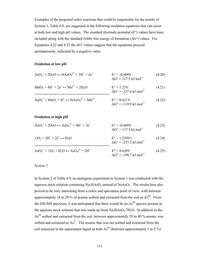
111
Examples of the proposed redox reactions that could be responsible for the results of
System 1, Table 4.9, are suggested in the following oxidation equations that can occur
at both low and high pH values. The standard electrode potential (E°) values have been
included along with the standard Gibbs free energy of formation (∆G°) values. For
Equations 4.22 and 4.25 the ∆G° values suggest that the equations proceed
spontaneously, indicated by a negative value.
Oxidation at low pH
AsO2¯ + 2H2O ↔ HAsO4
2¯ + 3H+ + 2e¯ E° = -0.609V (4.20) ∆G° = 117.5 kJ mol-1 MnO2 + 4H+ + 2e¯ ↔ Mn2+ + 2H2O E° = 1.23V (4.21) ∆G° = -237.4 kJ mol-1 AsO2¯ + MnO2 + H+ ↔ HAsO4
2¯ + Mn2+ E° = 0.621V (4.22) ∆G° = -119.9 kJ mol-1 Oxidation at high pH AsO2¯ + 2H2O ↔ AsO4
3¯ + 4H+ + 2e¯ E° = -0.609V (4.23) ∆G° = 117.5 kJ mol-1 ½O2 + 2H+ + 2e¯ ↔ H2O E° = 1.229V) (4.24) ∆G° = -237.2 kJ mol-1 AsO2¯ + ½O2 + H2O ↔ AsO4
3¯ + 2H+ E° = 0.620V (4.25) ∆G° = -199.7 kJ mol-1
System 2
In System 2 of Table 4.9, an analogous experiment to System 1 was conducted with the
aqueous stock solution containing Na2HAsO4 instead of NaAsO2. The results here also
proved to be very interesting from a redox and speciation point of view, with between
approximately 18 to 29 % of arsenic sorbed and extracted from the soil as AsIII. From
the ESI-MS spectrum, it was anticipated that there would be no AsIII species present in
the aqueous stock solution that was made up from Na2HAsO4.7H2O. In addition to the
AsIII sorbed and extracted from the soil, between approximately 29 to 40 % arsenic was
sorbed and extracted as AsV. The arsenic that was not sorbed and extracted from the
soil remained in the supernatant liquid as both AsIII (between approximately 1 to 5 %)
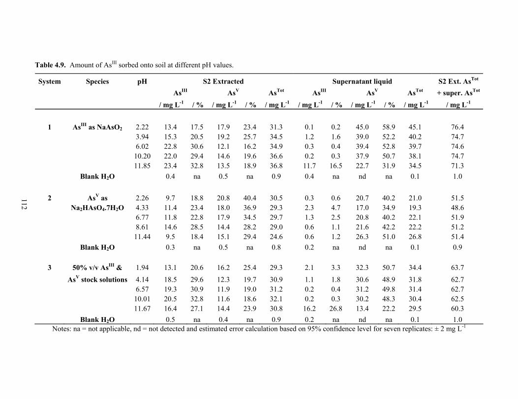
112
Table 4.9. Amount of AsIII sorbed onto soil at different pH values.
System Species pH S2 Extracted Supernatant liquid S2 Ext. AsTot AsIII AsV AsTot AsIII AsV AsTot + super. AsTot
/ mg L-1 / % / mg L-1 / % / mg L-1 / mg L-1 / % / mg L-1 / % / mg L-1 / mg L-1
1 AsIII as NaAsO2 2.22 13.4 17.5 17.9 23.4 31.3 0.1 0.2 45.0 58.9 45.1 76.4 3.94 15.3 20.5 19.2 25.7 34.5 1.2 1.6 39.0 52.2 40.2 74.7 6.02 22.8 30.6 12.1 16.2 34.9 0.3 0.4 39.4 52.8 39.7 74.6 10.20 22.0 29.4 14.6 19.6 36.6 0.2 0.3 37.9 50.7 38.1 74.7 11.85 23.4 32.8 13.5 18.9 36.8 11.7 16.5 22.7 31.9 34.5 71.3 Blank H2O 0.4 na 0.5 na 0.9 0.4 na nd na 0.1 1.0
2 AsV as 2.26 9.7 18.8 20.8 40.4 30.5 0.3 0.6 20.7 40.2 21.0 51.5 Na2HAsO4.7H2O 4.33 11.4 23.4 18.0 36.9 29.3 2.3 4.7 17.0 34.9 19.3 48.6 6.77 11.8 22.8 17.9 34.5 29.7 1.3 2.5 20.8 40.2 22.1 51.9 8.61 14.6 28.5 14.4 28.2 29.0 0.6 1.1 21.6 42.2 22.2 51.2 11.44 9.5 18.4 15.1 29.4 24.6 0.6 1.2 26.3 51.0 26.8 51.4 Blank H2O 0.3 na 0.5 na 0.8 0.2 na nd na 0.1 0.9
3 50% v/v AsIII & 1.94 13.1 20.6 16.2 25.4 29.3 2.1 3.3 32.3 50.7 34.4 63.7 AsV stock solutions 4.14 18.5 29.6 12.3 19.7 30.9 1.1 1.8 30.6 48.9 31.8 62.7 6.57 19.3 30.9 11.9 19.0 31.2 0.2 0.4 31.2 49.8 31.4 62.7 10.01 20.5 32.8 11.6 18.6 32.1 0.2 0.3 30.2 48.3 30.4 62.5 11.67 16.4 27.1 14.4 23.9 30.8 16.2 26.8 13.4 22.2 29.5 60.3 Blank H2O 0.5 na 0.4 na 0.9 0.2 na nd na 0.1 1.0 Notes: na = not applicable, nd = not detected and estimated error calculation based on 95% confidence level for seven replicates: ± 2 mg L-1

113
0.0
5.0
10.0
15.0
20.0
25.0
30.0
35.0
40.0
0.00 1.00 2.00 3.00 4.00 5.00 6.00 7.00 8.00 9.00 10.00 11.00 12.00 13.00
pH
% A
sIII e
xtra
cted
from
S2
a
b
c
Figure 4.22. A plot of % AsIII extracted from S2 versus pH: (a) AsIII as NaAsO2
species, (b) AsV as Na2HAsO4 species and (c) 50% v/v mixture of AsIII and AsV
stock solutions.
0.0
5.0
10.0
15.0
20.0
25.0
30.0
35.0
40.0
45.0
0.00 1.00 2.00 3.00 4.00 5.00 6.00 7.00 8.00 9.00 10.00 11.00 12.00 13.00
pH
% A
sV e
xtra
cted
from
S2
c
a
b
Figure 4.23. A plot of % AsV extracted from S2 versus pH: (a) AsIII as NaAsO2
species, (b) AsV as Na2HAsO4 species and (c) 50% v/v mixture of AsIII and AsV
stock solutions.
114
and AsV (between approximately 35 to 51 %). The detection of AsIII sorbed and
extracted from the soil suggests that something in the soil causes the AsV to be reduced
to AsIII. This phenomenon does not take place in the absence of soil as shown in the
results in Table 4.8.
An explanation for the results of System 2, Table 4.9, is that under oxic conditions,
arsenic is primarily found as AsV, which sorbs strongly to Fe and Al (hydr)oxides
[322,326,354-356]. Surface-bound arsenic is released into solution under slightly
reducing conditions through the reductive dissolution of the Fe (hydr)oxides [357-359].
Arsenate reduction to highly toxic AsIII may accompany its release into solution [360-
362].
Postulated reduction equations at low and high pH values, in the presence of FeIII and
sulfides, are suggested below. The E° and ∆G° values have been included to support
the notion that the equations proceed spontaneously.
Reduction at low pH 4x (HAsO4
2¯ + 3H+ + 2e¯ ↔ AsO2¯ + 2H2O) E° = 4 (0.609V) = 2.436V (4.26) ∆G° = -1880.3 kJ mol-1 S2¯ + 4H2O ↔ SO4
2¯ + 8H+ + 8e¯ E° = -0.149V (4.27) ∆G° = 115.0 kJ mol-1 4HAsO4
2¯ + 4H+ + S2¯ ↔ 4AsO2¯ + SO42¯ + 4H2O E° = 2.287V (4.28)
∆G° = -1765.3 kJ mol-1 Reduction at high pH AsO4
3¯ + 4H+ + 2e¯ ↔ AsO2¯ + 2H2O E° = 0.609V (4.29) ∆G° = -117.5 kJ mol-1 2x (Fe3+ + e- ↔ Fe2+) E° = 2(0.770V) = 1.54V (4.30) ∆G° = -297.2 kJ mol-1 Equation 4.29 and Equation 4.30 can be added together as follows: AsO4
3¯ + 4H+ + 4e¯ + 2Fe3+ ↔ AsO2¯ + 2H2O + 2Fe2+ E° = 2.149V (4.31) ∆G° = -414.7 kJ mol-1 If Equation 4.31 is multiplied by 2 it can be reduced using the following equation:
115
S2¯ + 4H2O ↔ SO42¯ + 8H+ + 8e¯ E° = -0.149V (4.32)
∆G° = 115.0 kJ mol-1 2AsO4
3¯ + S2¯ + 2Fe3+ ↔ 2AsO2¯ + SO42¯ + 4Fe2+ E° = 4.149V (4.33)
∆G° = -3202.6 kJ mol-1
System 3
In System 3 of Table 4.9, the aqueous stock solution contained a 50% v/v mixture of
AsIII and AsV stock solutions. Not surprisingly, the results for System 3 are found to be
consistent with those of System 1, in that, when the pH is high the percentage AsIII
sorbed and extracted by the soil is generally highest. The opposite is observed for
oxidation, with more AsIII being oxidised at lower pH, as reflected in the soil extract and
more particularly in the supernatant.
In summary, both oxidative and reductive processes have been established as a result of
exposure of AsIII/AsV to a light clay in aqueous media over a range of pH values. It is
evident that specific sorption sites on the light clay are able to sorb, oxidise/reduce and
desorb AsIII/AsV species in varying amounts according to the pH of the system.
Generally, the maximum sorption and extraction of AsIII occurs at an almost neutral pH
for NaAsO2 compared to a relatively basic pH for Na2HAsO4 species. On the other
hand, the maximum sorption and extraction of AsV generally occurs at relatively low pH
values.

116
5.0 Conclusions & Future Directions
5.1 Conclusions
A statistical analysis of data entered into a database revealed the relative abundances of
metals and, in particular, arsenic within soils of various geological units. These units
included the Quaternary Aeolian (Qpw, highest concentration of zinc, lowest
concentration of chromium) the Quaternary Fluvial (Qrc, highest chromium and nickel
concentrations, equal highest copper, lowest lead and equal lowest arsenic
concentrations); the Quaternary Newer Volcanics (Qvn, equal lowest arsenic
concentration); Silurian Anderson Creek Formation (Sla, highest arsenic concentration);
Silurian Dargile Formation (Sud, highest lead and equal highest copper concentrations);
Tertiary Brighton Group (Tpb, lowest nickel concentration) and Older Volcanics (Tvo,
lowest copper and zinc concentrations).
A detailed review of the current literature has exposed a number of limitations in
conducting comparisons between different inorganic background soil constituent data.
Namely, issues associated with non-standardised sampling strategies (i.e. single versus
bulked/composited samples), varying sampling depths, differing soil sampling
intensities, sampling location strategies which vary randomly or systematically, and data
obtained using different analytical techniques, were identified. In particular, it was
found that most studies present chemical constituent data as a total concentration that
provides limited information about the chemical species that are present and the
bioavailability of those species. A particular limitation of inorganic background soil
data in the literature includes the failure to relate the data to targeted geological regions.
Initial arsenic soil sorption experiments revealed that the average percentage AsTot
sorbed depends on the soil type. Thus clay loam, light clay and silt loam were found to
sorb approximately 19.6%, 2.9% and 38.2% respectively, whereas the sand sorbed
negligible arsenic, with concentrations below the method detection limit. A second
sorption study that allowed for a longer exposure time revealed optimum arsenic
sorption concentrations. Under these conditions the clay loam, light clay, sand and silt
loam sorbed approximately 76 %, 84 %, 2.4 % and 72 % respectively. These results
were found to relate to the clay content, pH and EC values. This is consistent with
literature data confirming that the material substrate plays a vital role in the sorption of

117
arsenic (i.e. higher clay content soils sorb the most arsenic) with the pH of the system
also playing a significant role in determining the amount of arsenic sorbed. The results
of the current study also confirm that soils with higher arsenic sorption qualities
generally exhibit higher concentrations of extractable Fe and Al. Iron present in these
soils is likely to be in the form of iron (hydr)oxides that has been extensively identified
in the literature as being a most suitable sorption material for arsenic.
The experimental results obtained in the present work revealed that the extent of
sorption of arsenic in soils is highly dependent on the time of sorption. The
concentration of sorbed arsenic increases rapidly in the first 30 min and then continues
to increase more slowly thereafter, approaching a maximum sorption concentration.
The sorption has been modelled using a two-step kinetic process.
An in vitro bioavailability technique was evaluated to assess its applicability in
determining the relative bioavailability of arsenic when sorbed onto four different soil
types. The technique demonstrated a clear differentiation in the relative bioavailabilities
of the four soil types and illustrated the dependence of arsenic bioavailability on the
physical and chemical properties of the soil. For the clay loam, light clay, sand and silt
loam the relative arsenic bioavailability was determined to be approximately 32%, 80%,
100% and 60% respectively. The sorption process in these studies was not an
equilibrium process since the ratio for the percentage arsenic bioavailability to the
percentage arsenic non-bioavailability varied with the spiked concentration. The
calculated ratios cannot be considered to be partition coefficients since they do not
remain constant with various spike concentrations. A plot of the percentage arsenic
bioavailability versus the concentration of arsenic delivered in the spike reveals that the
bioavailability is limited in a non-linear way by the loading capacity of the soil. These
plots also illustrate that different soil types result in different bioavailability profiles. A
novel technique was implemented to estimate, for each soil type, the apparent partition
coefficient that is obtained as the concentration of arsenic in the spike approaches zero.
The apparent limiting partition coefficients for the clay loam, light clay and silt loam are
0.255, 2.228 and 0.809 respectively.
The observation that (except for sand) the maximum percentage bioavailability ranged
from approximately 32 to 80 % is in contrast with a number of studies in the literature
that assume that close to 100% of soluble arsenic is sorbed by the human
118
gastrointestinal tract. This tacit assumption is questionable given that arsenic in soil is
expected to be incompletely extracted during transit through the gastrointestinal tract.
In a global sense, a simple gastric relative bioavailability technique provides a valuable
estimation for the bioavailability characteristics of a given soil. Such a technique
provides quick and readily available information on the relative bioavailability of
arsenic in soils without the need for conducting ethically questionable, expensive and
time-consuming in vivo bioavailability experiments. Simple models, like the one used
in this study, rely on the fact that although arsenic is sorbed through the intestinal
epithelium, the rate-controlling step in arsenic sorption is dissolution in the stomach.
As a result, complicated gastrointestinal models do not necessarily estimate relative
bioavailability better than the simpler gastric models.
Several techniques were employed to investigate and evaluate the speciation of
phosphorus (as a benchmark) and arsenic under a variety of conditions, including
gaseous/in vacuo, solution and soil. The utility of ESI-MS for the qualitative and
quantitative assessment of arsenic and phosphorus speciation in solution was evaluated
to identify and characterize these species. The technique demonstrated considerable
potential for the study of both phosphorus and arsenic speciation, particularly for
qualitative speciation analyses in solution. From the qualitative data, various postulates
were formulated for the interaction between different species. For the speciation of
phosphorus using ESI-MS, HPO42¯ in the presence of hydronium ions was postulated to
form PO3¯ and water. The continued reaction of PO3¯ to form H2PO4¯ was also
proposed to account for the experimental observations. A similar mechanism to that of
phosphorus was also proposed to account for the experimental observations made on the
analogous arsenic species. In this case, ESI-MS was also used to identify and
characterise arsenite species in solution. From these results, a mechanism for the
formation of the H2AsO3¯ species from AsO2¯ in the presence of water was postulated.
In the process of ESI-MS speciation analyses, a novel technique was developed to assay
the “oxidative purity” of an aqueous arsenite sample. The ESI-MS results revealed that
the supplied arsenite salt contained the following oxidative impurities: AsO43¯, AsO3¯,
H2AsO3¯ and H2AsO4¯. The ESI-MS technique proved to be a most suitable technique
for identification of such oxidative impurities in an aqueous sample and can be
recommended to be used for this purpose in future investigations of this nature.
119
The species identified in ESI-MS were modelled using high-level density functional
calculations with the aim of providing supporting evidence for the postulated reaction
mechanisms. The reaction energies for the two phosphorus mechanisms were -267.02
and -25.13 kcal mol-1 indicating an equilibrium shift to the right-hand side in both cases,
favouring the PO3¯ and H2PO4¯ species in their respective reactions. Using analogous
calculations to those of phosphorus, the calculated reaction energies for the arsenate
systems were -265.10 and -22.30 kcal mol-1, with the equilibrium shift in both cases
towards the right-hand side, favouring the AsO3¯ and H2AsO4¯ species. For the arsenite
system the calculated reaction energy was -70.84 kcal mol-1, favouring the formation of
the H2AsO3¯ species. These novel, modelled reaction energy calculations proved in all
cases to be a favourable method in supporting the postulated mechanisms arising from
the ESI-MS results.
As part of the species energy and reaction energy calculations, a number of computer-
generated geometries for the phosphorus and arsenic species were obtained and were
found to compare favourably with reported crystallographic data. Along with these
computer-generated geometries, structures for each of the identified ESI-MS
phosphorus and arsenic species were also modelled. The computer-generated structures
for XO3¯ (X = P, As) indicated perfect trigonal planar geometries with a delocalize
electron configuration. For HXO42¯ and H2XO4¯ species the structures exhibited
varying degrees of distorted tetrahedral geometries. In light of the computer-generated
structures, it was discovered that the H2XO4¯ species exhibited isomers, predicated on
the existence of strong intramolecular hydrogen bonds, with the hydrogen atoms located
in either cis or trans positions relative to each other. In the case of the arsenite species,
computer structures for AsO2¯ and H2AsO3¯ proved to be extremely interesting. The
structure of AsO2¯ exhibited a linear geometry with a delocilised electron configuration.
Whereas, the structure for H2AsO3¯ exhibited four possible isomeric structures with
increasing energies in the following order: pyramidal H2AsO3¯ < cis-T-shaped (planar)
H2AsO3¯ < tetrahedral H2AsO3¯ (with one hydrogen directly bonded to the central
arsenic atom) < trans-T-shaped (planar) H2AsO3¯. These isomers seem not to have been
reported previously in the literature and represent significant finds with respect to
arsenic speciation.
Modelled HOMO and LUMO data revealed the order of decreasing reactivity for the
phosphorus and arsenic species investigated: HPO42¯ > HAsO4
2¯ > AsO2¯ > H2AsO3¯
120
>PO3¯ > H2PO4¯ > AsO3¯ > H2AsO4¯. It is postulated that the HOMO of each of these
phosphorus and arsenic species is likely to form bonds with the LUMO of other species
that might be present in the soil or water environments. In this regard, the more reactive
species are likely to sorb to soil particles. This facilitates hypotheses to be proposed for
the distribution of such species in solution and also provides insight into how these
species may be taken up into a clay structure. The computer modelled calculations also
yielded electrostatic potential energy maps for each of the phosphorus and arsenic
species which serve to quickly characterise various regions within a molecular species
as being electron rich, electron poor, or neither rich nor poor, based on a colour scale.
A novel technique was adopted to quantify the purity of an AsIII sample and to
determine the amount of AsIII sorbed onto soil under different pH conditions. The
technique is based on a previously reported speciation technique that utilizes the known
preference of halogenated AsIII to be extracted into chloroform. The purity of the AsIII
sample, using this technique, was demonstrated to be approximately 86 % with the
remaining 14 % corresponding to the “oxidative impurities” that were qualitatively
identified using ESI-MS. Using this extraction technique, the quantitative amount of
AsIII sorbed onto soil under different pH conditions was also measured in order to
provide insight into the behaviour of AsIII species when taken up by the soil. The
results for an AsIII sample revealed that approximately 17 to 33 % of AsIII was sorbed
and extracted by the soil with < 1 to 16.5 % AsIII remaining in the supernatant liquid.
The remainder of the AsIII was oxidized (possibly by manganese oxides or by aerobic
oxidation processes) to AsV and was either sorbed and extracted by the soil (~16 to 26
%) or remained oxidized in the supernatant liquid (~32 to 59 %). The sorption and
oxidation characteristics taking place in the soil were found to be pH dependent, with
higher AsIII sorption taking place at higher pH. For the oxidation process, more AsIII is
oxidised at lower pH.
For the AsV system, approximately 18 to 29 % was sorbed and extracted as AsIII, with
approximately 1 to 5 % AsIII remaining in the supernatant liquid. The remainder of the
AsV was either sorbed and extracted by the soil (~28 to 40 %) or remained in the
supernatant liquid (~35 to 51 %) as AsV. The detection of AsIII in a soil soaked in an
AsV solution suggests that the soil is capable of reducing some of the AsV into AsIII. It
was proposed that such a reduction could be facilitated by the presence of FeIII and
sulfides that are present in the soil. From these results it is evident that specific sorption
121
sites on the clay are able to sorb, oxidize/reduce and desorb AsIII/AsV species in varying
amounts according to the pH of the system. It was found that the maximum sorption
and extraction of AsIII occurs at almost neutral pH and that the sorption and extraction
of AsV occurs at a relatively low pH. These experimental results thus provide valuable
information on the nature of the species in the soil, the possible redox processes taking
place and the pH dependency of such processes.
5.2 Future Directions
The research has created new pathways that can be explored to continue the quest to
elucidate the complex nature of arsenic sorption in, and bioavailability from, soils. It is
anticipated that further research in the following areas could be undertaken in the future:
(i) The determination of the relationship between the kinetics described in Section 4.2
with the bioavailability (Section 4.3) and speciation (Section 4.4). Such work could
provide valuable information as to whether arsenic is kinetically bioavailable to humans
and also provide an insight into the speciation kinetics.
(ii) The determination of arsenic speciation using ESI-MS is a promising method that
could be investigated further by the development of soil extraction techniques and by
the optimization of instrumental parameters to enable the instrumental speciation to
reflect, as accurately as possible, the actual speciation in the extract. In addition, it is
envisaged that techniques involving ESI-MS could also be developed for the
quantitative analysis of individual arsenic species derived from soil matrices.
(iii) A continuation of computer modelling investigations for phosphorus and arsenic
species, especially those identified by ESI-MS, is an area of ongoing interest. The
existence of various isomers is of particular interest since little is known about how this
relates to their (environmental) chemistry and biochemistry. It is also desirable for such
isomers to be isolated in the laboratory for experimental evaluation.
122
6.0 References [1] San Juan, C., (1994), Natural Background Soil Metal Concentrations in
Washington State. Publication No. 94 – 115, October 1994. The United States
Geological Survey and the Washington State Department of Ecology.
[2] Duchaufour, P., (1977). Pedology. George Allen & Unwin, London.
[3] Kabata-Pendias, A., Dudka, S., Chlopecka, A. and Gawinowska, T., (1992).
Background levels and environmental influences on trace metals in soils of the
temperate humid zone of Europe, In: Biogeochemistry of trace metals, Ed.
Adriano, D. C., Lewis Publishers, U.S.A.
[4] National Environment Protection (Assessment of Site Contamination) Measure
1999, Schedule B(1) – Guideline on Investigation Levels for Soil and
Groundwater, Section 5.2 Background Variation, pp 7.
[5] Australian and New Zealand Environment and Conservation Council
(ANZECC) and National Health and Medical Research Council (NHMRC).
(1992). Australian and New Zealand Guidelines for the Assessment and
Management of Contaminated Sites.
[6] McKeague, J. A. and Wolynetz, M. S., (1980). Background levels of minor
elements in some Canadian soils, Geoderma, 24, 299-307.
[7] Yan-Chu, H., (1994). Arsenic distribution in soils, In: Arsenic in the
environment, Part 1: Cycling and characterisation, Ed. Nriagu, J. O., John Wiley
& Sons, New York, pp 17-49.
[8] Sadiq, M., Zaidi, T. H. and Main, A., (1983). Environmental behaviour of
arsenic in soils: Theoretical, Water, Air, Soil Pollut., 20 (4), 369-377.
[9] Li, S. Z., Wang, W. X., Li, E. G. and Dun, S. Q., (1981). A preliminary study of
the fixation of methanearsonate herbicides in Hutuo river drainage soils, China
123
Environ. Sci., 1, 41-45.
[10] Li, X. G., (1982). Chemical forms and content of arsenic in some soils of China,
Turang Xuebao, 19 (4), 360-366.
[11] Koyama, T. and Shibuya, M., (1976). Soil-plant relation studies on arsenic. II.
Correlation between easily extractable arsenate in soils and the response of rice
plants, Nippon Dojo Hiryogaku Zasshi, 47 (3), 93-98.
[12] Norimoto, W., and Osamu, H., (1982). Adsorption of arsenite and arsenate by
soils and charcoal, Kankyo Gijutsu, 11 (8), 565-571.
[13] Xu, H., Allard, B. and Grimvall, A., (1988). Influence of pH and organic
substances on the absorption of arsenic(V) on geological materials, Water, Air,
Soil Pollut., 40 (3-4), 293-305.
[14] Galba, J. and Polacek, S., (1973). Sorption of arsenates under kinetic conditions
in selected soil types, Acta Fytotech., 28, 187-197.
[15] Micheal, B. A. and Russell, J. L., (1976). Chemical distribution and gaseous
evolution of arsenic-74 added to soils arsenic-74-labeled DSMA, Soil Sci. Soc.
Am. J., 40 (5), 655-658.
[16] Ruby, M. V., Davis, A., Schoof, R., Eberle, S. and Sellstone, C. M., (1996).
Estimation of Lead and Arsenic Bioavailability Using a Physiologically Based
Extraction Test, Environ. Sci. Technol., 30, 422-430.
[17] Walsh, L. M. and Keeney, D. R., (1975). Behaviour and phytotoxicity of
inorganic arsenicals in soils, ACS Symp. Ser. 7, 35-52.
[18] Xie, Z. M., Zhu, Z. X., Yuan, K. N. and Huang, C. Y., (1989). Effect of
birnessite (δ-MnO2) on oxidation of arsenic(III) in soils, Huanjing Huaxue, 8 (2),
1-6.
[19] Tournassat, C., Charlet, L., Bosbach, D. and Manceau, A., (2002). Arsenic(III)
124
oxidation by birnessite and precipitation of manganese(II) arsenate, Environ.
Sci. Technol., 36, 493-500.
[20] Oscarson, D. W., Huang, P. M., Defosse, C. and Herbillion, A., (1981).
Oxidative power of Mn(IV) and Fe(III) oxides with respect to As(III) in
terrestrial and aquatic environments, Nature, 191, 50-51.
[21] Helgesen, H and Larsen, E. H., (1998). Bioavailability and speciation of arsenic
in carrots grown in contaminated soil, Analyst, 123, 791-796.
[22] Hayes, K. F. and Traina, S. J., (1998). In: Soil Chemistry and Ecosystem Health,
Special Publication 52, Soil Science Society of America.
[23] Huang, P. M. and Fujii, R., (1998). In: Chemical Methods. Methods of Soil
Analysis, Part 3, Book Series No. 5, Soil Science Society of America.
[24] Bissen, M. and Frimmel, F. H., (2000). Speciation of As(III), As(V), MMA and
DMA in contaminated soil extracts by HPLC-ICP/MS, Fresenius J. Anal.
Chem., 367, 51-55.
[25] Ferguson, and Gavis, (1972). A review of the arsenic cycle in natural waters,
Water Res., 6 (11), 1259-1274.
[26] Webb, J. L. (Ed.), (1976). Enzyme and metabolic inhibitors, Academic Press,
New York.
[27] Deuel, L. E. and Swoboda, A. R., (1972). Arsenic solubility in a reduced
environment, Soil Sci. Soc. Am. Pro., 36, 276-278.
[28] Cullen, W. R. and Reimer, K. J., (1989). Arsenic speciation in the environment,
Chem. Rev., 89, 713–764.
[29] Takamatsu, T., Aoki, H. and Yoshida, T., (1982). Determination of arsenate,
arsenite, monomethylarsenate, and dimethylarsenate in soil polluted with
arsenic, Soil Sci., 133, 239-246.

125
[30] Pohl, B., and Bächmann, K., (1986). Fresenius J. Anal. Chem., 323, 859-865.
[31] Bhumbla, D. K. and Keefer, R. F., (1994). Arsenic mobilization and
bioavailability in soils, In: Arsenic in the environment, Part 1: Cycling and
characterisation, Ed. Nriagu, J. O., John Wiley & Sons, New York, pp 51-82.
[32] Chappell, J., Chiswell, B. and Olszowy, H., (1995). Speciation of arsenic in a
contaminated soil by solvent extraction, Talanta, 42 (3), 323-329.
[33] Pongratz, R., (1998). Arsenic speciation in environmental samples of
contaminated soil, Sci. Tot. Environ., 224, 133-141.
[34] Pantsar-Kallio, M. and Manninen, P. K. G., (1997). Speciation of mobile arsenic
in soil samples as a function of pH, Sci. Tot. Environ., 204, 193-200.
[35] Landrum, P. F., Hayton, W. L., et al., (1992), Bioavailability: Physical,
Chemical and Biological Interactions, Session 6, Chapter 3, Synopsis of
discussion session on the kinetics behind environmental bioavailability,
Thirteenth Pellston Workshop, Pellston, Michigan, August 17-22, Lewis
Publishers.
[36] Newman, M. C. and Jagoe, C. H., (1992), Bioavailability: Physical, Chemical
and Biological Interactions, Session 3, Chapter 1, Ligands and the bioavailability
of metals in aquatic environments, Thirteenth Pellston Workshop, Pellston,
Michigan, August 17-22, Lewis Publishers.
[37] Benson, W. H. and Alberts, J. J., (1992), Bioavailability: Physical, Chemical
and Biological Interactions, Session 3, Chapter 2, Synopsis of discussion session
on the bioavailability of inorganic contaminants, Thirteenth Pellston Workshop,
Pellston, Michigan, August 17-22, Lewis Publishers.
[38] Peijnenburg, W. J. G. M., Posthuma, L., Eijsackers, H. J. P. and Allen H. E.,
(1997), A Conceptual Framework for Implementation of Bioavailability of
Metals for Environmental Management Purposes, Ecotoxicol. Environ. Saf., 37,
126
163-172.
[39] Ruby, M. V., Schoof, W. B, Brattin, W., Goldade, M., Post, G., Harnois, M.,
Mosby, D. E., Casteel, S. W., Berti, W., Carpenter, M., Edwards, D., Cragin, D.
and Chappell, W., (1999). Advances in Evaluating the Oral Bioavailability of
Inorganics in Soil for Use in Human Health Risk Assessment, Environ. Sci.
Technol., 33, 3697-3705.
[40] Williams, T. M., Rawlins, B. G., Smith, B. and Breward, N., (1998). In-Vitro
Determination of Arsenic Bioavailability in Contaminated Soil and Mineral
Beneficiation Waste from Ron Phibun, Southern Thailand: A Basis for Improved
Human Risk Assessment, Environ. Geochem. Health., 20, 169-177.
[41] Ruby, M. V., Davis, A., Link, T. E., Schoof, R., Chaney, R. L., Freeman, G. B.
and Bergstrom, P., (1993). Development of an in vitro screening test to evaluate
the in vivo bioaccessibility of ingested mine-waste lead, Environ. Sci. Technol.,
27 (13), 2870-2877.
[42] Ng, J. C., Kratzmann, S. M., Qi, L., Crawley, H., Chiswell, B. and Moore, M.
R., (1998). Speciation and absolute bioavailability: risk assessments of arsenic-
contaminated sites in a residential suburb in Canberra, Analyst, 123, 889-892.
[43] Das, A. K., Chakraborty, R., Cervera, M. L. and de la Guardia, M., (1995).
Metal speciation in solid matrices, Talanta, 42, 1007-1030.
[44] de la Guardia, M., (1996). Non-Chromatographic Methods for the Element
Speciation by Atomic Spectrometry, In: Element Speciation in Bioinorganic
Chemistry, Ed. Caroli, S., Wiley-Interscience.
[45] Kot, A. and Namiesnil, J., (2000). The role of speciation in analytical chemistry,
Trends Anal. Chem., 19 (2-3), 69-79.
[46] Templeton, D. M., Ariese, F., Cornelis, R., Danielsson, L. G., Huntan, H., Van
Leeuwen, H. P., (2000). Guidelines for terms related to chemical speciation and
fractionation of elements. Definitions, structural aspects, and methodological
127
approaches (IUPAC Recommendations 2000), Pure Appl. Chem., 72 (8), 1453-
1470.
[47] Bradley, R. I., (1980). Trace Elements in Soils around Llechryd, Dyfed, Wales,
Geoderma, 24, 17-23.
[48] Davies, B. E., (1985). Baseline Survey of Metals in Welsh Soils, Environmental
Geochemistry and Health, I. Thornton, Ed., London, p 16-17.
[49] McGrath, S. P., (1987). Computerized Quality Control, Statistics and Regional
Mapping of the Concentrations of Trace and Major Elements in the Soils of
England and Wales, Soil Use and Management, 3, 31-38.
[50] McGrath, S. P., Cunliffe, C. H. and Pope, A. J., (1985). Lead, Zinc, Cadmium,
Copper, Nickel Concentrations in the Topsoils of England and Wales,
Environmental Geochemistry and Health, I. Thornton, Ed., London, p 16-17.
[51] Archer, F. C. and Hodgson, J. H., (1987). Total and Extractable Trace Element
Contents of Soils in England and Wales, J. Soil Sci., 38, 421-431.
[52] Thornton, I., (1991). Metal contamination of soils in urban areas, In Soils in the
urban environment, Ed. Bullock, P., Blackwell Scientific Publications, 1991,
Chapter 4, pp 47-75.
[53] Aubert, M. and Pinta, M., (1977). Trace Elements in Soils, Amsterdam: Elsevier,
pp 395.
[54] Chen, T. B., Wong, J. W. C., Zhou, H. Y. and Wong, M. H., (1996). Assessment
of Trace Metal Distribution and Contamination in Surface Soils of Hong Kong,
Environ. Pollut., 96 (1), 61-68.
[55] Bini, C., Dall’Aglio, M., Ferretti, O. and Gragnani, R., (1988). Background
Levels of Microelements in Soils of Italy, Environ. Geochem. Health, 10 (2), 63-
69.
128
[56] Angelone, M. and Bini, C., (1992). Trace Elements Concentrations in Soils and
Plants of Western Europe, Printed in Biogeochemistry of Trace Metals, Ed.
Domey C. Adriano, Lewis Publishers, Chapter Two, pp 19-60.
[57] Aller, A. J. and Deban, L., (1989). Total and Extractable Contents of Trace
Metals in Agricultural Soils of the Valderas Area, Spain, Sci. Total Environ., 79,
253-270.
[58] Shacklette, H. T., Hamilton, J. C., Boerngen, J. C. and Bowles, J. M., (1971).
Elemental Composition of Surficial Material in the United States, U.S. Geol.
Surv. Prof. Pap., 574D.
[59] Vinogradov, A. P., (1959). The Geochemistry of Rare and Dispersed Chemical
Elements in Soils, 2nd Edition, Consultants Bureau, New York, N.Y.
[60] Tiller, K. G., de Vries, M. P. C., Spouncer, L. R., Smith, L. H., and Zarcinas, B.,
(1976). Environmental pollution of the Port Pirie region, Metal contamination of
home gardens with city and then vegetable produce, CSIRO Division of Soils
Div. Rep. No. 15.
[61] Smith, L. H. and Tiller, K. G., (year unknown). Unpublished work referred to in
Tiller, K. G., (1992), Urban Soil Contamination in Australia, Aust. J. Soil Res.,
30, 937-957.
[62] Tiller, K.G., (1992). Urban Soil Contamination in Australia, Table 4
‘Background’ Concentrations of Heavy Metals in Urban Soils from Non-
industrial Sites, Aust. J. Soil Res., 30, 944-957.
[63] Olszowy, H., Torr, P., and Imray, P., (1995). Trace Element Concentrations in
Soils from Rural and Urban Areas of Australia, Contaminated Sites Monograph
Series No. 4, South Australian Health Commission, pp 1-11.
[64] Lawrie, R. A., Keneally, J. P. and Stevens, M. L., (1992). Background Trace
Elements in Soils around Sydney, Fourth National Soils Conference – Soil
Protection and Productivity, Adelaide, South Australia, pp 19-23.
129
[65] Torr, P., and Alphen, M., (1993). Background Urban Levels of Heavy Metals in
Surface Soils, Contaminated Sites Monograph Series No. 4, South Australian
Health Commission, pp 65-87.
[66] Davis, A., Sherwin, D., Ditmars, R. and Hoenke, A., (2001). An Analysis of
Soil Arsenic Records of Decision, Environ. Sci. Technol., 35 (12), 2401-2406.
[67] Davies, B. E., (1992). Trace Metals in the Environment: Retrospect and
Prospect, In Biogeochemistry of Trace Metals, Ed. Adriano, D. C., Lewis
Publishers, Chelsea,
MI., U.S.A.
[68] Alloway, B. J., (1995), The Origins of Heavy Metals in Soils. In: Heavy Metals
in Soils, Ed. Alloway, B. J., Blackie Academic & Professional, 1995. Chapter 3,
pp 38-57.
[69] Dragun, J. and Chekiri, K., (2005). Elements in North American Soils, Amherst
Scientific Publishers, Amherst, Massachusetts, U.S.A.
[70] McGrath, S. P., (1995). Chromium and Nickel, Chapter 7, In: Heavy Metals in
Soils, Ed. Alloway, B. J., Blackie Academic & Professional, pp 152-178.
[71] O’Neill, P., (1995). Arsenic, Chapter 5, In: Heavy Metals in Soils, Ed. Alloway,
B. J., Blackie Academic & Professional, London, pp 105-121.
[72] Lottermoser, B., (1997). Heavy metal pollution of Australian soils, Search, 28
(3), 91-93.
[73] U.S. Department of Agriculture, Natural Resources Conservation Service,
(2003). National Soil Survey Handbook, Title 430-VI [Online –
www.soils.usda.gov/technical/handbook].
[74] Unified Soil Classification System, USCS, (2000), American Society for Testing
and Materials, D2487-00 Standard Classification of Soils for Engineering

130
Purposes.
[75] Holtz, R.D. and Kovacs, W.D. (1981). An Introduction to Geotechnical
Engineering, Chapter 3, Prentice Hall.
[76] American Association of State Highways and Transportation (AASHTO)
(1978). Standard specifications for transportation materials and methods of
sampling and testing. AASHTO Designation: M 145-73, 12th ed. Washington,
D.C.: AASHTO.
[77] Federal Aviation Administration (FAA) (1967). Airport Paving. Washington
D.C.: FAA.
[78] American Society for Testing and Materials, (2002). D422-63(2002) Standard
Test Method for Particle-Size Analysis of Soils.
[79] Lambe, T. W., and Whitman, R. V., (1969). Soil Mechanics, Massachusetts
Institute of Technology, John Wiley & Sons, New York, NY.
[80] Northcote, K. H., (1971). A Factual Key for the Recognition of Australian Soils,
3rd Edition, Rellim Technical Publications.
[81] Singh, D.B., Prasad, G. and Rupainwar, D.C., (1996). Adsorption technique for
the treatment of As(V)-rich effluents, Colloids Surfaces A: Physicochem. Eng.
Aspects 111, 49-56.
[82] Singh, D. B., Gupta, G. S., Rupainwar, D. C. and Prasad, G., (1993). J. Environ.
Sci. Health, Part 1, 28, 1813.
[83] Genc-Fuhrman, H., Tjell, J. C. and McConchie, D., (2004). Adsorption of
Arsenic from Water Using Activated Neutralized Red Mud, Environ. Sci.
Technol., 38, 2428-2434
[84] Matis, K. A., Zouboulis, A. I., Zamboulis, D. and Valtadorou, V., (1999).
Sorption of As(V) by Goethite Particles and Study of their Flocculation, Water,
131
Air, and Soil Pollution, 111, 297-316.
[85] Genc, H., Tjell, J. C., McConchie, D. and Schuiling, O., (2003). Adsorption of
arsenate from water using neutralized red mud, J. Colloid Interface Sci., 264(2),
327-334.
[86] Zeng, L., (2003). A method for preparing silica-containing iron(III) oxide
adsorbents for arsenic removal, Water Research, 37, 4351-4358
[87] Singh, D.B., Prasad, G., Rupainwar, D.C. and Singh, V.N., (1988). As(III)
Removal from Aqueous Solution by Adsorption, Water, Air & Soil Pollut., 42,
337-386.
[88] Mckay, G., El Geundi, M. and Nassar, M. M., (1988). External mass transport
processes during the adsorption of dyes onto bagasse pith, Water Res., 22, 1527-
1533.
[89] Gupta, G.S., Prasad, G. and Singh, V.N., (1988). J. Environ. Sci. Health, A23,
205.
[90] Stumm, W., (1992). Chemistry of the Solid Water Interface, Wiley & Sons, New
York.
[91] Altundogan, H. S., Altundogan, S., Tumen, F. and Bildik, M., (2000). Arsenic
removal from aqueous solutions by adsorption on red mud, Waste Manage., 20,
761-767.
[92] Arai, Y., Elzinga, E. J. and Sparks, D., (2001). X-ray Absorption Spectroscopic
Investigation of Arsenite and Arsenate Adsorption at the Aluminum Oxide–
Water Interface, J. Colloid Interface Sci., 235, 80-88.
[93] Goldberg, S. and Johnston C. T., (2001). Mechanisms of Arsenic Adsorption on
Amorphous Oxides Evaluated Using Macroscopic Measurements, Vibrational
Spectroscopy, and Surface Complexation Modeling, J. Colloid Interface Sci.,
234, 204-216.
132
[94] Yang, J. K., Barnett, M., Jardine, P. M. and Casteel, S. W., (2002). Adsorption,
Sequestration, and Bioaccessibility of As(V) in Soils, Environ. Sci. Technol., 36,
4562-4569
[95] Raven, K. P., Jain, A., Loeppert, R. H., (1998). Arsenite and Arsenate
Adsorption on Ferrihydrite: Kinetics, Equilibrium, and Adsorption Envelopes,
Environ. Sci. Technol., 32, 344-349.
[96] Prasad, G., (1994). In Arsenic in the Environment, Part I: Cycling and
Characterization, Nriagu, J. O. (Ed.), Removal of Arsenic(V) from aqueous
system by adsorption onto some geological materials, Wiley and Sons, New
York.
[97] Stumm, W., (1987). Aquatic Surface Chemistry – Chemical Processes at the
Particle-Water Interface, Wiley and Sons, New York.
[98] Zhang, J. and Stanforth, R., (2005). Slow Adsorption Reaction between Arsenic
Species and Goethite (r-FeOOH): Diffusion or Heterogeneous Surface Reaction
Control, Langmuir, 21, 2895-2901
[99] Jain, A., Raven, K. P. and Loeppert, R. H., (1999). Arsenite and Arsenate
Adsorption on Ferrihydrite: Surface Charge Reduction and Net OH- Release
Stoichiometry, Environ. Sci. Technol., 33, 1179-1184.
[100] Arai, Y., Sparks, D. L. and Davis, J. A., (2004). Effects of Dissolved Carbonate
on Arsenate Adsorption and Surface Speciation at the Hematite-Water Interface,
Environ. Sci. Technol., 38, 817-824.
[101] Sun, X. H. and Doner, H. E., (1996). An Investigation of Arsenate and Arsenite
Bonding Structures on Goethite by FTIR, Soil Sci., 161, 865.
[102] Cornell, R. M. and Schwertmann, U., (2003). The Iron Oxides: Structure,
Properties, Reactions, Occurrence and Uses, 2nd ed., Wiley-VCH: Weinheim,
Germany.
133
[103] Fuller, C. C., Davis, J. A. and Waychunas, G. A., (1993). Surface chemistry of
ferrihydrite: Part 2. Kinetics of arsenate adsorption and coprecipitation,
Geochim. Cosmochim. Acta, 57, 2271-2282.
[104] O’Reilly, S. E., Strawn, D. G. and Sparks, D. L., (2001). Residence time effects
on arsenate adsorption/desorption mechanisms on goethite, Soil Sci. Soc. Am. J.,
65, 67-78.
[105] Waltham, C. A. and Eick, M. J., (2002). Kinetics of arsenic adsorption on
goethite in the presence of sorbed silicic acid, Soil Sci. Soc. Am. J., 66, 818-826.
[106] Woolson, E. A., Axley, J. H. and Kearney, P. C., (1971). Soil Sci. Soc. Am.
Proc., 35, 101.
[107] Wauchope, R. D., and McDowell, L. L., (1984). J. Environ. Qual., 13, 499.
[108] Sun, X. and Doner, H. E., (1998). Adsorption and oxidation of arsenite on
goethite, Soil Sci., 163 (4), 278–287.
[109] Theis, T. L., Iyer, R. and Ellis, S. K., (1992). Evaluating a new granular iron
oxide for removing lead from drinking water, J. Am. Water Works Assoc., 84,
101-105.
[110] Anderson, P. and Benjamin, M. M., (1985). Effects of silicon on the
crystallization and adsorption properties of ferric oxides, Environ. Sci. Technol.,
19, 1048-1053.
[111] Swedlund, P. J. and Webster, J. G., (1999). Adsorption and polymerization of
silicic acid on ferrihydrite, and its effect on arsenic adsorption, Water Res., 33
(16), 3413-3422.
[112] Manning, B. A. and Goldberg, S., (1996). Clay Clay Miner., 44 (5), 609-623.
[113] Gao, Y. and Mucci, A., (2001). Acid base reactions, phosphate and arsenate
134
complexation, and their competitive adsorption at the surface of goethite in 0.7
M NaCl solution, Geochim. Cosmochim. Acta., 65 (14), 2361-2378.
[114] Wilkie, J. A. and Hering, J. G., (1996). Adsorption of arsenic onto hydrous
ferric oxide: effects of adsorbate/adsorbent ratios and co-occurring solutes,
Colloids Surf., A, 107, 97-110.
[115] Holm, T. R., (2002). Effects of CO32-/bicarbonate, Si, and PO43¯ on arsenic
sorption to HFO, J. Am. Water Works Assoc., 94 (4), 174-181.
[116] Redman, A. D., Macalady, D. L. and Ahmann, D., (2002). Natural Organic
Matter Affects Arsenic Speciation and Sorption onto Hematite, Environ. Sci.
Technol., 36, 2889-2896.
[117] Genc¸ H. and Tjell, J. C., (2003). J. Phys. IV, 107, 537-540.
[118] Gregor, J., (2001). Arsenic removal during conventional aluminium-based
drinking-water treatment, Water Res., 35 (7), 1659-1664.
[119] Edwards, M., (1994). J. Am. Water Works Assoc., 86 (9), 64-78.
[120] Bajpai, S. and Chaudhuri, M., (1999). Removal of Arsenic from Ground Water
by Manganese Dioxide-Coated Sand, J. Environ. Engin., 125 (8), 782-784.
[121] Kanel, S. R., Manning, B., Charlet, L. and Choi, H., (2005). Removal of
Arsenic(III) from Groundwater by Nanoscale Zero-Valent Iron, Environ. Sci.
Technol., 39, 1291-1298.
[122] Tseng, W. P., (1977). Effects and dose-response relationships of skin cancer and
blackfoot disease with arsenic, Environ. Health Perspect., 19, 109-119.
[123] U.S. EPA. (1992). Relative absorption factors for risk assessment. U.S.
Environmental Protection Agency, Exposure Assessment Group, Washington,
DC.
135
[124] Freeman, G. B., Schoof, R. A., Ruby, M. V., Davis, A. O., Dill, J. A., Liao, S.
C., Lapin, C. A. and Bergstrom, P. D., (1996). Bioavailability of arsenic in soil
and house dust impacted by smelter activities following oral administration in
Cynomolgus monkeys, Fund. Appl. Toxicol., 28 (2), 215-222.
[125] Sarkar, D., and Datta, R., (2003). New initiatives: A modified in-vitro method
to assess bioavailable arsenic in pesticide-applied soil, Environ. Pollut., 126,
363-366.
[126] Basta, N. T., Rodriguez, R. R and Casteel, S. W., (2002). Bioavailability and
risk of arsenic exposure by the soil ingestion pathway, Chapter 5, In
Environmental Chemistry of Arsenic, Edi. Frankenberger, W. T., Marcel Dekker
Inc., New York.
[127] Davis, A., Ruby, M. V., Bloom, M., Schoof, R., Freeman, G. and Bergstrom, P.
D., (1996). Mineralogic Constraints on the Bioavailability of Arsenic in Smelter-
Impacted Soils, Environ. Sci. Technol., 30, 392-399.
[128] Davis, A., V. Ruby, M. V. and Bergstrom, P. D., (1992). Bioavailability of
Arsenic and Lead in Soils from the Butte, Montana, Mining District, Environ.
Sci. Technol., 26, 461-468.
[129] Rodriguez, R. R., Basta, N. T., Casteel, S. and Pace, L., (1999). An In Vitro
Gastrointestinal Method to Estimate Bioavailable Arsenic in Contaminated Soils
and Solid Media, Environ. Sci. Technol., 33, 642-649.
[130] Freeman, G. B., Johnson, J. D., Killinger, J. M., Liao, S. C., Davis, A. O., Ruby,
M. V., Chaney, R. L., Lovre, S. C., Bergstrom, P. D. (1993). Fundam. Appl.
Toxicol., 21, 83-88.
[131] Freeman, G. B., Johnson, J. D., Liao, S. C., Feder, P. I., Davis, A. O., Ruby, M.
V., Schoof, R. A., Chaney, R. L. and Bergstrom, P. D., (1994). Toxicology, 91,
151-163.
[132] Sarkar, D., and Datta, R., (2003). New initiatives: A modified in-vitro method
136
to assess bioavailable arsenic in pesticide-applied soil, Environ. Pollut., 126,
363-366.
[133] Oomen, A. G., Hack, A., Minekus, M., Zeijdner, E., Cornelis, C., Schoeters, G.,
Verstraete, W., Van De Wiele, T., Wragg, J., Rompelberg, C. J. M., Sips, A. J.
A. M. and Van Wijnen, J. H., (2002). Comparison of five in vitro digestion
models to study the bioaccessibility of soil contaminants, Environ. Sci. Technol.,
36, 3326-3334.
[134] Hunter, J. M., (1973). Geophagy in Africa and in the United States: A culture-
nutrient hypothesis, Geographical Review, 63 (2), 170-195.
[135] Drover, D. P. and Borrell, W., (1980). Analysis of two edible clays from East
Sepik, Papua New Guinea, Science in New Guinea, 7 (1), 6-11.
[136] Lake, D.L., Kirk, P.W.W. and Lester, J.N., (1984). Fractionation,
characterisation, and speciation of heavy metals in sewage sludge and sludge-
amended soils: A review, J. Environ. Qual., 13, 175-183.
[137] Gong, Z., Lu, X., Ma, M., Watt, C. and Le, C., (2002). Arsenic speciation
analysis, Talanta, 58, 77-96.
[138] Zhang, H., Davison, W., Miller, S. and Tych, W., (1995). In situ high resolution
measurements of fluxes of Ni, Cu, Fe and Mn and concentrations of Zn and Cd
in porewaters by DGT, Geochim. Cosmochim. Acta, 59, 4181-4191.
[139] Zhang, H., Davison, W., Knight, B. and McGrath, S., (1998). In situ
measurements of solution concentrations and fluxes of trace metals in soils using
DGT, Environ. Sci. Technol., 32, 704-710.
[140] Hooda, P. S., Zhang, H., Davison, W. and Edwards, A. C., (1999). Measuring
bioavailable trace metals by diffusive gradients in thin films (DGT): soil
moisture effects on its performance in soils, Eur. J. Soil Sci., 50, 285-294.
[141] Zhang, H., Zhao, F., Sun, B., Davison, W. and McGrath, S. P., (2001). A new
137
method to measure effective soil solution concentration predicts copper
availability to plants, Environ. Sci. Technol., 35, 2602-2607.
[142] Jones, A. D., Supplement 5: Partition Equilibria: Henry’s Law and Octanol-
water Partition Equilibria important concepts for environmental chemistry,
Review Materials for Chemistry 402, The Pennsylvania State University.
[143] IUPAC Compendium of Chemical Terminology, Second Edition (1993). 65,
2385.
[144] Perin, G., Fabris, R., Manente, S., Rebello Wagener, A., Hamacher, C. and
Scotto, S., (1997). A five-year study on the heavy-metal pollution of Guanabara
Bay sediments (Rio De Janeiro, Brazil) and evaluation of the metal
bioavailability by means of geochemical speciation, Water Res., 31, 3017-3028.
[145] Hansch, C. and Fujita, T., (1964). p-σ-π Analysis. A Method for the correlation
of biological activity and chemical structure, J. Am. Chem. Soc., 86, 1616-1625.
[146] Leo, A., Hansch, C. and Elkins, D., (1971). Partition Coefficients and their Uses,
Chem. Rev., 71, 525-616.
[147] Hansch, C. and Leo, A., (1979). Substituent Constants for Correlation Analysis
in Chemistry and Biology, Wiley, New York.
[148] Chou, J. T. and Jurs, P. C., (1979). Computer-assisted computation of partition
coefficient from molecular structures using fragment constants. J. Chem. Inf.
Comput. Sci., 19, 172-178.
[149] Leo, A., (1990). In Comprehensive Medicinal Chemistry, Hansch, C. (Ed),
Pergamon: Oxford, 4, 295-319.
[150] Rekker, R. F. (1977). The Hydrophobic Fragment Constant, Elsevier: New
York.
[151] Suzuki, T. and Kudo, Y., (1990). Automatic log P estimation based on combined
138
additive modeling methods, J. Comput.-Aided Mol. Des., 4, 155-198.
[152] Klopman, G. and Wang, S., (1991). A Computer Automated Structure
Evaluation (CASE) Approach to Calculation of Partition Coefficient, J. Comput.
Chem., 12, 1025-1032.
[153] Klopman, G, Li, J., Wang, S. and Dimayuga, M., (1994). Computer Automated
log P Calculations Based on an Extended Group Approach, J. Chem. Inf.
Comput. Sci., 34, 752-781.
[154] Broto, P., Moreau, G. and Vandycke, C., (1984). Molecular structures:
perception, autocorrelation descriptor and SAR studies, Eur. J. Med. Chem., 19,
71-78.
[155] Ghose, A. K. and Crippen, G. M., (1986). Atomic Physicochemical Parameters
for Three-Dimensional Structure-Directed Quantitative Structure-Activity
Relationships. I. Partition Coefficients as a Measure of Hydrophobicity, J.
Comput. Chem., 7, 565-577.
[156] Ghose, A. K., Pritchett, A. and Crippen, G. M., (1988). Atomic Physicochemical
Parameters for Three-Dimensional Structure-Directed Quantitative Structure-
Activity Relationships. III. Modelling Hydrophobic Interactions, J. Comput.
Chem., 9, 80-90.
[157] Klopman, G. and Iroff, L. D., (1981). Calculation of Partition Coefficients by the
Charge Density Method, J. Comput.Chem., 2, 157-160.
[158] Bodor, N., Gabanyi, Z. and Wong, C. K., (1989). A New Method for the
Estimation of Partition Coefficient, J. Am. Chem. Soc., 111, 3783-3786.
[159] Wang, R., Fu, Y. and Lai, L., (1997). A New Atom-Additive Method for
Calculating Partition Coefficients, J. Chem. Inf. Comput. Sci., 37 (3), 615-621.
[160] Liang, J. and Schoenau, J. J., (1996). Speciation in metal contaminated soils as
revealed by an ion exchange resin membrane fractionation procedure, Commun.
139
Soil Sc. Plant Anal., 27 (18 – 20), 3013-3026.
[161] Lebourg, A., Sterckeman, T., Ciesielski, H. and Proix, N., (1998). Trace metal
speciation in three unbuffered salt solutions used to assess their bioavailability in
soil, J. Environ. Qual., 27, 584-590.
[162] Conder, J. M., Lanno, R. P. and Basta, N. T., (2001). Assessment of metal
availability in smelter soil using earthworms and chemical extractions, J.
Environ. Qual., 30 (4), 1231-1238.
[163] Corbisier, P., Van der Lelie, D., Borremans, B., Provoost, A., De Lorenzo, V.,
Brown, N. L., Lloyd, J. R., Hobman, J. L., Csoregi, E., Johansson, G. and
Mattiasson, B., (1999). Whole cell- and protein-based biosensors for the
detection of bioavailable heavy metals in environmental samples, Anal. Chim.
Acta, 387, 235-244.
[164] Agemian, H. and Chau, A. s., (1976). Evaluation of extraction techniques for the
determination of metals in aquatic sediments, Analyst, 101, 761-767.
[165] Tessier, A., Campbell, P. G. and Bisson, M., (1979). Sequential extraction
procedure for the speciation of particulate trace metals, Anal. Chem., 51, 844-
851.
[166] Gatehouse, S., Russel, D.W. and van Moort, J.C., (1977). Sequential soil
analysis in exploration geochemistry, J. Geochem. Explor., 8, 483-494.
[167] Sposito, G., Lund, L.J. and Chang, A.C., (1982). Trace metal chemistry in arid-
zone field soils amended with sewage sludge: I. Fractionation of Ni, Cu, Zn, Cd,
and Pb in solid phases, Soil. Sci. Soc. Am. J., 46, 260-264.
[168] Miller, W.P., and McFee, W.W., (1983). Distribution of Cd, Zn, Cu, and Pb in
soils of industrial northwestern Indiana, J. Environ. Qual., 12, 29-33.
[169] Bermond, A., Yousfi, I. and Ghestem, J., (1998). Kinetic approach to the
chemical speciation of trace metals in soils, Analyst, 123, 785-789.
140
[170] Marin, B., Valladon, M., Polve, M. and Monaco, A., (1997). Reproducibility
testing of a sequential extraction scheme for the determination of trace metal
speciation in a marine reference sediment by inductively coupled plasma-mass
spectrometry, Anal. Chim. Acta, 342, 91-112.
[171] Psenner, R., Pucsko, R. and Sager, M., (1984). Arch. Hydro-biol. Suppl., 70,
111-115.
[172] Shuman, L.M. and Hargrove, W.L., (1985). Effect of tillage on the distribution
of manganese, copper, iron, and zinc in soil fractions, Soil. Sci. Soc. Am. J., 49,
1117-1121.
[173] Kersten, M. and Forstner, U., (1986). Chemical fractionation of heavy metals in
anoxic estuarine and coastal sediments, Water Sci. Technol., 18, 121-130.
[174] Zeien, H. and Brummer, G.W., (1989). Mitt. Dt. Bodenkundl. Ges., 59, 505-
510.
[175] Hirner, A.V., Kritsotakis, K. and Tobschall, H.J., (1990). Metal-organic
associations in sediments. Comparison of unpolluted recent and ancient
sediments and sediments affected by anthropogenic pollution, Appl. Geochem.,
5, 491-505.
[176] Chester, R. and Huges, M. J., (1967). A chemical technique for the separation of
ferro-manganese minerals, carbonate minerals and adsorbed trace elements from
pelagic sediments, Chem. Geol., 2, 249-262.
[177] Ho, M. D. and Evans, G. J., (1997). Operational speciation of cadmium, copper,
lead and zinc in the NIST standard reference material 2710 and 2711 (Montana
soil) by the BCR sequential extraction procedure and flame atomic absorption
spectrometry, Anal. Commun., 34, 363-364.
[178] Adriano, D. C., (2001). Trace Elements in Terrestrial Environments, 2nd Edition,
Springer, New York.
141
[179] Wenzel, W. W., Kirchbaumer, N., Prohaska, T., Stingeder, G., Lombi, E. and
Adriano, D. C., (2001). Arsenic fractionation in soils using an improved
sequential extraction procedure, Anal. Chim. Acta, 436, 309-323.
[180] Shiowatana, J., McLaren, R. G., Chanmekha, N. and Samphao, A., (2001).
Fractionation of arsenic in soil by a continuous-flow sequential extraction
method, J. Environ. Qual., 30 (6), 1940-1949.
[181] Johnston, S. E. and Barnard, W. M., (1979). Comparative effectiveness of
fourteen solutions for extracting As from four western New York soils, Soil Sci.
Soc. Am. J., 43, 304.
[182] Polyak, K. and Hlavay, J., (1999). Environmental mobility of trace metals in
sediments collected in the Lake Balaton, Fresenius J. Anal. Chem., 363, 587-
593.
[183] Marin, A., Lopez-Gonzalvez, A., and Barbas, C., (2001). Development and
validation of extraction methods for determination of zinc and arsenic speciation
in soils using focused ultrasound: Application to heavy metal study in mud and
soils, Anal. Chim. Acta, 442, 305-318.
[184] Szpunar, J., (2000). Bio-inorganic speciation analysis by hyphenated techniques,
Analyst, 15, 963-988.
[185] Guerin, T., Astruc, A., and Astruc, M., (1999). Review Speciation of arsenic and
selenium compounds by HPLC hyphenated to specific detectors: a review of the
main separation techniques, Talanta, 50, 1-24.
[186] Timberbaev, A. R., (2000). Review Element speciation analysis by capillary
electrophoresis, Talanta, 52, 573-606.
[187] Kolbl, G., Kalcher, K, and Irgolic, K., (1993). Ion chromatography
determination of selenite and selenate-specific detection by flame and graphite
furnace atomic absorption spectrometry, Anal. Chim. Acta, 284, 301-310.
142
[188] Szpunar-Lobinska, J., Witte, C., Lobinski, R., and Adams, F., (1995). Fresenius
J. Anal. Chem., 351, 351.
[189] Beauchemin, D., Siu, K., McLaren, J., Berman, S., (1989). Determination of
arsenic species by high-performance liquid chromatography-inductively coupled
plasma mass spectrometry, J. Anal. At. Spectrom., 4 (3), 285-289.
[190] Cai, Y., Cabanas, M., Fernandez-Turiel, J., Abalos, M., and Boyona, J., (1995).
On-line preconcentration of selenium(IV) and selenium(VI) in aqueous matrices
followed by liquid chromatography-inductively coupled plasma mass
spectrometry determination, Anal. Chim. Acta, 314, 183.
[191] Li, K., Li, S. F. Y., (1995). Speciation of selenium and arsenic compounds in
natural waters by capillary zone electrophoresis after on-column
preconcentration with field-amplified injection, Analyst, 120, 361-366.
[192] Naidu, R., Smith, J., McLaren, R. G., Stevens, D. P., Sumner, M. E. and
Jackson, P. E., (2000). Application of capillary electrophoresis to anion
speciation in soil water extracts: II. Arsenic, Soil Sci. Soc. Am. J., 64, 122.
[193] Tomlinson, M. J., Lin, L. and Caruso, J. A., (1995). Plasma mass spectrometry
as a detector for chemical speciation studies, Analyst, 120, 583-589.
[194] Morita, M., Uehiro, T. and Fuwa, K., (1981). Determination of arsenic
compounds in biological samples by liquid chromatography with inductively
coupled argon plasma-atomic emission spectrometric detection, Anal. Chem.,
53, 1806.
[195] Tye, C. T., Haswell, S. J., O’Neill, P. and Bancroft, K. C. C., (1985). High
performance liquid chromatography with hydride generation/atomic absorption
spectrometry for the determination of arsenic species with application to some
water samples, Anal. Chim. Acta, 169, 195.
143
[196] Morita, M. and Shibata, Y., (1987). Speciation of arsenic compounds in marine
life by high performance liquid chromatography combined with inductively
coupled argon plasma atomic emission spectrometry, Anal. Sci., 3, 575.
[197] Maitani, T., Uchiyama, S. and Saito, Y., (1987). Hydride generation-flame
atomic-absorption spectrometry as an arsenic detector for high-performance
liquid chromatography, J. Chromatogr. A, 391, 161-168.
[198] Shiomi, K., Orii, M., Yamanaka, H. and Kikuchi, T., (1987). Nippon Suisan
Gakkaishi, 53, 103.
[199] Heitkemper, D., Creed, J., Caruso, J. and Fricke, F. L., (1989). Speciation of
arsenic in urine using high-performance liquid chromatography with inductively
coupled plasma mass spectrometric detection, J. Anal. At. Spectrom., 4 (3), 279-
284.
[200] Ricci, G. R., Shepard, L. S., Colovos, G. and Hester, N. E., (1981). Ion
chromatography with atomic absorption spectrometric detection for
determination of organic and inorganic arsenic species, Anal. Chem., 53 (4),
610-613.
[201] Brinckman, F. E., Jewett, K. L., Iverson, W. P., Irgolic, K. J., Ehrhardt, K. C.
and Stockton, R. A., (1980). Graphite furnace atomic absorption
spectrophotometers as automated element-specific detectors for high-pressure
liquid chromatography: The determination of arsenite, arsenate, methylarsonic
acid and dimethylarsinic acid, J. Chromatogr. A, 191, 31-46.
[202] Kurosawa, S., Yasuda, K., Tagushi, M., Yamazaki, S., Toda, S., Morita, M.,
Uehiro, T. and Fuwa, K., (1980). Agric. Biol. Chem., 44, 1993.
[203] Iadevaia, R., Aharonson, N. and Woolson, E. A., (1980). J. Assoc. Off. Anal.
Chem., 63, 742.
144
[204] Roychowdhury, S. B. and Koropchak, J. A., (1990). Thermospray enhanced
inductively coupled plasma atomic emission-spectroscopy detection for liquid
chromatography, Anal. Chem., 62 (5), 484-489.
[205] Spall, W. D., Lynn, J. G., Andersen, J. L., Valdez, J. G. and Gurley, L. R.,
(1986). High-performance liquid chromatographic separation of biologically
important arsenic species utilizing on-line inductively coupled argon plasma
atomic emission spectrometric detection, Anal. Chem., 58, 1340.
[206] Branch, S., Bancroft, K. C. C., Ebdon, L. and O’Neill, P., (1989). Anal. Proc.,
26, 73.
[207] Shibata, Y. and Morita, M., (1989). Speciation of arsenic by reverse-phase high
performance liquid chromatography-inductively coupled plasma mass
spectrometry, Anal. Sci., 5, 107.
[208] Beauchemin, D., Bednas, M. E., Berman, S. S., McLaren, J. W., Siu, K. W. M.
and Sturgeon, R. E., (1988). Identification and quantitation of arsenic species in
a dogfish muscle reference material for trace elements, Anal, Chem., 60 (20),
2209-2212.
[209] Francesconi, K. A., Micks, P., Stockton, R. A., and Irgolic, K. J., (1985).
Quantitative determination of arsenobetaine, the major water-soluble arsenical in
three species of crab, using high pressure liquid chromatography and an
inductively coupled argon plasma emission spectrometer as the arsenic-specific
detector, Chemosphere, 14 (10), 1443.
[210] Stocktan, R. A., and Irgolic, K. J., (1979). Int. J. Environ. Anal. Chem., 6, 313.
[211] Nisamaneepong, W., Ibrahim, M., Gilbert, W., and Caruso, J. A., (1984). J.
Chromatogr. Sci., 22, 473.
[212] Low, G.K.-C., Batley, G. E., and Buchanan, S. J., (1986). Application of column
switching in high-performance liquid chromatography to arsenic speciation
145
analysis with inductively coupled argon plasma spectrometric detection, J.
Chromatogr., 368, 423.
[213] Wangkarn, S. and Pergantis, S. A., (2000). High-speed separation of arsenic
compounds using narrow-bore high-performance liquid chromatography on-line
with inductively coupled plasma mass spectrometry, J. Anal. At. Spectrom., 15,
627-633.
[214] Do, B., Robinet, S., Pradeau, D. and Guyon, F., (2001). Speciation of arsenic
and selenium compounds by ion-pair reversed-phase chromatography with
electrothermic atomic absorption spectrometry: Application of experimental
design for chromatographic optimisation, J. Chromatogr. A, 918, 87-98.
[215] Manning, B. A. and Martens, D. A., (1997). Speciation of Arsenic(III) and
Arsenic(V) in Sediment Extracts by High-Performance Liquid Chromatography-
Hydride Generation Atomic Absorption Spectrophotometry, Environ. Sci.
Technol., 31 (1), 171-177.
[216] Howard, A. G. and Hunt, L. E., (1993). Coupled photooxidation-hydride AAS
detector for the HPLC of arsenic compounds, Anal. Chem., 65, 2995-2998.
[217] Capelo, J., Lavilla, I. and Bendicho, C., (2001). Ultrasonic Extraction Followed
by Sonolysis-Ozonolysis as a Sample Pretreatment Method for Determination of
Reactive Arsenic toward Sodium Tetrahydroborate by Flow Injection-Hydride
Generation AAS, Anal. Chem., 73, 3732-3736.
[218] Carrero, P., Malave, A., Luis Burguera, J., Burguera, M. and Rondon, C.,
(2001). Determination of various arsenic species by flow injection hydride
generation atomic absorption spectrometry: investigation of the effects of the
acid concentration of different reaction media on the generation of arsines, Anal.
Chim. Acta, 438, 195-204.
[219] Shraim, A., Chiswell, B. and Olszowy, H., (2000). Use of perchloric acid as a
reaction medium for speciation of arsenic by hydride generation–atomic
absorption spectrometry, Analyst, 125, 949-953.
146
[220] Ebdon, L., Hill, S. and Ward, R. W., (1987). Directly coupled chromatography-
atomic spectroscopy. Part 1. Directly coupled gas chromatography-atomic
spectroscopy. A review, Analyst, 111, 1113-1138.
[221] Blais, J.-S., Momplaisir, G.-M., and Marshall, W. D., (1990). Determination of
arsenobetaine, arsenocholine, and tetramethylarsonium cations by HPLC
thermochemical hydride generation-atomic absorption spectrometry, Anal.
Chem., 62 (11), 1161-1166.
[222] Bermejo-Barrera, P., Barciela-Alonso, C., Ferron-Novais, M and Bermejo-
Barrera, A., (1995). Speciation of arsenic by the determination of total arsenic
and arsenic(III) in marine sediment samples by electrothermal atomic absorption
spectrometry, J. Anal. At. Spectrom., 10, 247-252.
[223] Chausseau, M., Roussel, C., Gilon, N. and Mermet, J. M., (2000). Optimization
of HPLC-ICP-AES for the determination of arsenic species, Fresenius’ J. Anal.
Chem., 366, 476-480.
[224] Weeger, W., Lievremont, D., Perret, M., Lagarde, F., Hubert, J. C., Leroy, M.
and Lett, M. C., (1999). Oxidation of arsenite to arsenate by a bacterium isolated
from an aquatic environment, Biometals, 12, 141-149.
[225] Rauret, G., Rubio, R. and Padro, A., (1991). Fresenius’ J. Anal. Chem., 340,
157.
[226] Rubio, R., Padro, A., Alberti, J. and Rauret, G., (1992). Mikrochim. Acta, 109,
39-44.
[227] Gettar, R. T., Garavaglia, R. N., Gautier, E. A. and Batistoni, D. A., (2000).
Determination of inorganic and organic anionic arsenic species in water by ion
chromatography coupled to hydride generation–inductively coupled plasma
atomic emission spectrometry, J. Chromatogr. A, 884, 211-221.
147
[228] Do, B., Alet, P., Pradeau, D., Poupon, J., Guilley-Gaillot, M. and Guyon, F.,
(2000). On-line reversed-phase liquid chromatography hydride generation
emission spectrometry: speciation of arsenic in urine of patients intravenously
treated with As2O3, J. Chromatogr. B, 740, 179-186.
[229] Thompson, J. J., and Houk, R. S., (1986). Inductively coupled plasma mass
spectrometric detection for multielement flow injection analysis and elemental
speciation by reversed-phase liquid chromatography, Anal. Chem., 58 (12),
2541-2548.
[230] Yehl, P., and Tyson, J. F., (1997). Towards Speciation of Arsenic in a Standard
Reference River Sediment by High-performance Ion Chromatography Coupled
With Plasma Source Mass Spectrometry, Anal. Commun., 34 (2), 49-51.
[231] Geiszinger, A., Goessler, W., Kuehnelt, D., Francesconi, K. and Kosmus, W.,
(1998). Determination of Arsenic Compounds in Earthworms, Environ. Sci.
Technol., 32 (15), 2238-2243.
[232] Byrdy, F. A. and Caruso, J. A., (1995). Trace metals speciation by HPLC with
plasma source mass spectrometry detection, Environ. Health Perspect. Suppl.,
103 (1), 21.
[233] Vela, N. P. and Caruso, J. A., (1993). The potential of LC-ICP-MS for trace
metal speciation, J. Anal. At. Spectrom., 8, 787-794.
[234] Zybin, A., Schaldach, G., Berndt, H. and Niemax, K., (1998). Metal speciation
in the ppt range by HPLC and diode laser atomic absorption spectrometry in a
flame, Anal. Chem., 70, 5093-5096.
[235] Van Holderbeke, M., Zhao, Y., Vanhaecke, F., Moens, L., Dams, R. and Sandra,
P., (1999). Speciation of six arsenic compounds using capillary electrophoresis-
inductively coupled plasma mass spectrometry, J. Anal. At. Spectrom., 14, 229-
234.
148
[236] Magnuson, M.L., Creed, M. T. and Brockhoff, C. A., (1997). Speciation of
Arsenic Compounds in Drinking Water by Capillary Electrophoresis with
Hydrodynamically Modified Electroosmotic Flow Detected Through Hydride
Generation Inductively Coupled Plasma Mass Spectrometry With a Membrane
Gas–Liquid Separator, J. Anal. At. Spectrom., 12, 689-695.
[237] Prange, A. and Schaumloffel, D., (1999). Determination of element species at
trace levels using capillary electrophoresis-inductively coupled plasma sector
field mass spectrometry, J. Anal. At. Spectrom., 14, 1329-1332.
[238] Le, X. C., Lu, X., Ma, M., Cullen, W. R., Aposhian, H. V. and Zheng, B.,
(2000). Speciation of Key Arsenic Metabolic Intermediates in Human Urine,
Anal. Chem., 72, 5172-5177.
[239] Le, X. C. and Ma, M., (1998). Short-Column Liquid Chromatography with
Hydride Generation Atomic Fluorescence Detection for the Speciation of
Arsenic Anal. Chem. 70, 1926-1933.
[240] Bohari, Y., Astruc, A., Astruc, M. and Cloud, J., (2001). Improvements of
hydride generation for the speciation of arsenic in natural freshwater samples by
HPLC-HG-AFS, J. Anal. At. Spectrom., 16, 774-778.
[241] Vilano, M., Padro, A. and Rubio, R., (2000). Coupled techniques based on liquid
chromatography and atomic fluorescence detection for arsenic speciation, Anal.
Chim. Acta, 411, 71-79.
[242] Corr, J. J. and Larsen, E. H., (1996). Arsenic speciation by liquid
chromatography coupled with ionspray tandem mass spectrometry, J. Anal. At.
Spectrom., 11, 1215-1224.
[243] Shibata, Y. and Morita, M., (1989). Exchange of comments on identification and
quantitation of arsenic species in a dogfish muscle reference material for trace
elements, Anal. Chem., 61, 2116-2118.
149
[244] Corr, J. J., (1997). Measurement of Molecular Species of Arsenic and Tin Using
Elemental and Molecular Dual Mode Analysis by Ionspray Mass Spectrometry,
J.Anal. At. Spectrom., 12, 537-546.
[245] Pergantis, S. A., Winnik, W. and Betowski, D., (1997). Determination of Ten
Organoarsenic Compounds Using Microbore High-performance Liquid
Chromatography Coupled With Electrospray Mass Spectrometry-Mass
Spectrometry, J. Anal. At. Spectrom., 12, 531-536.
[246] Inoue, Y., Date, Y., Sakai, T., Shimizu, N., Yoshida, K., Chen, H., Kuroda, K.
and Endo, G., (1999). Identification and quantification by LC-MS and LC-ICP
MS of arsenic species in urine of rats chronically exposed to dimethylarsinic
acid (DMAA), Appl. Organomet. Chem., 13, 81-89.
[247] Florencio, M. H., Duarte, M. F., De Bettencourt, A. M. M., Gomes, M. L. and
Vilas, L. F., (1997). Electrospray Mass Spectra of Arsenic Compounds, Rapid
Commun. Mass Spectrom., 11, 469-473.
[248] Pedersen, S. N. and Francesconi, K. A., (2000). Liquid chromatography
electrospray mass spectrometry with variable fragmentor voltages gives
simultaneous elemental and molecular detection of arsenic compounds, Rapid
Commun. Mass Spectrom. 14, 641-645.
[249] McSheehy, S. and Szpunar, J., (2000). Speciation of arsenic in edible algae by
bi-dimensional size-exclusion anion exchange HPLC with dual ICP-MS and
electrospray MS/MS detection, J. Anal. At. Spectrom., 15, 79-87.
[250] Mcsheehy, S., Pohl, P., Lobinski, R. and Szpunar, J., (2001). Investigation of
arsenic speciation in oyster test reference material by multidimensional HPLC-
ICP-MS and electrospray tandem mass spectrometry (ES-MS-MS), Analyst,
126, 1055-1062.
[251] Gallagher, P. A., Wei, X., Shoemaker, J. A., Brockhoff, C. A. and Creed, J. T.,
(1999). Detection of arsenosugars from kelp extracts via IC-electrospray
150
ionization-MS-MS and IC membrane hydride generation ICP-MS, J. Anal. At.
Spectrom., 14, 1829-1834.
[252] Pergantis, S. A., Wangkarn, S., Francesconi, K. A. and Thomas-Oates, J. E.,
(2000). Identification of Arsenosugars at the Picogram Level Using
Nanoelectrospray Quadrupole Time-of-Flight Mass Spectrometry, Anal. Chem.,
72 (2), 357-366.
[253] Madsen, A. D., Goessler, W., Pedersen, S. N. and Francesconi, K. A., (2000).
Characterization of an algal extract by HPLC-ICP-MS and LC-electrospray MS
for use in arsenosugar speciation studies, J. Anal. At. Spectrom. 15, 657-662.
[254] Gallagher, P. A., Shoemaker, J. A., Wei, X., Brockhoff-Schwegel, C. A. and
Creed, J. T., (2001). Extraction and detection of arsenicals in seaweed via
accelerated solvent extraction with ion chromatographic separation and ICP-MS
detection, Fresenius’ J. Anal. Chem., 369, 71-80.
[255] Wang, J. and Marshall, W. D., (1994). Metal speciation by supercritical fluid
extraction with on-line detection by atomic absorption spectrometry, Anal.
Chem., 66, 3900-3907.
[256] Deng, B. and Chan, W., (2001). Metal speciation using capillary electrophoresis
– inductively coupled plasma atomic emission spectrometry and
polytetrafluoroethylene capillaries, Electrophoresis, 22, 2186-2191.
[257] Barnowski, C., Jakubowski, N., Stuewer, D., and Broekaert, J. A. C., (1997).
Speciation of chromium by direct coupling of ion exchange chromatography
with inductively coupled plasma mass spectrometry, J. Anal. At. Spectrom., 12,
1155-1161.
[258] Kalcher, K., Lintschinger, J., Gossler, W., Kolbl, G. and Novic, M., (1995).
Fresenius’ J. Anal. Chem., 351, 604.
[259] Tomlinson, M. J. and Caruso, J. A., (1996). Speciation of chromium using
thermospray nebulization as sample introduction into inductively coupled
151
plasma mass spectrometry, Anal. Chim. Acta, 322 (1), 1-9.
[260] Pantsar-Kallio, M. and Manninen, P. K. G., (1996). Speciation of chromium in
aquatic samples by coupled column ion chromatography-inductively coupled
plasma-mass spectrometry, Anal. Chim. Acta, 318 (3), 335-343.
[261] Forehand, T. J., Dupuy, A. E. and Tal, H., (1976). Determination of arsenic in
sandy soils, Anal. Chem., 48 (7), 999-1001.
[262] Beard, H. C. and Lyerly, L. A., (1961). Separation of arsenic from antimony and
bismuth by solvent extraction, Anal. Chem., 33 (12), 1781-1782.
[263] Greenwood, N. N. and Earnshaw, A., (1984). Chemistry of the Elements,
Pergamon Press, Oxford, pp 650-665.
[264] Holak, W. and Specchio, J. J., (1991). Determination of total arsenic, As(III) and
As(V) in foods by atomic absorption spectrometry, At. Spectrosc., 12 (4), 105-
108.
[265] Maher, W. A., (1981). Determination of inorganic and methylated arsenic
species in marine organisms and sediments, Anal. Chim. Acta, 126, 157-165.
[266] Maher, W. A., (1984). Mode of occurrence and speciation of arsenic in some
pelagic and estuarine sediments, Chem. Geol, 47, 333-345.
[267] Hansen, S. H., Larsen, E. h., Pritzl, G. and Cornett, C., (1992). Separation of
Seven Arsenic Compounds by High-performance Liquid Chromatography With
On-line Detection by Hydrogen-Argon Flame Atomic Absorption Spectrometry
and Inductively Coupled Plasma Mass Spectrometry, J. Anal. At. Spectrom., 7,
629-634.
[268] Hirner, A. V., (1992). Trace element speciation in soils and sediments using
sequential chemical extraction methods, Int. J. Environ. Anal. Chem., 46, 77-85.
[269] Foster, A. L., Brown, G. E. (Jr.), Tingle, T. N. and Parks, G. A., (1998).
152
Quantitative arsenic speciation in mine tailings using X-ray absorption
spectroscopy, Am. Mineral., 83, 553-568.
[270] Larsen, E. H., (1995). Fresenius’ J. Anal. Chem., 352, 582.
[271] Vergara Gallardo, M., Bohari, Y., Astruc, A., Potin-Gautier, M. and Astruc, M.,
(2001). Speciation analysis of arsenic in environmental solids Reference
Materials by high-performance liquid chromatography–hydride generation–
atomic fluorescence spectrometry following orthophosphoric acid extraction,
Anal. Chim. Acta, 441, 257-268.
[272] Demesmay, C. and Ollé, M., (1997). Application of microwave digestion to the
preparation of sediment samples for arsenic speciation, Fresenius J. Anal.
Chem., 357, 1116.
[273] Thomas, P., Finnie, J. K. and Williams, J. G., (1997). Feasibility of
Identification and Monitoring of Arsenic Species in Soil and Sediment Samples
by Coupled High-performance Liquid Chromatography - Inductively Coupled
Plasma Mass Spectrometry, J. Anal. Atom. Spectrom., 12, 1367-1372.
[274] Garcia-Manyes, S., Jimenez, G., Padro, A., Rubio, R. and Rauret, G., (2002).
Arsenic speciation in contaminated soils, Talanta, 58, 97-109.
[275] Pizarro, I., Gomez, M., Camara, C. and Palacios, M. A., (2003). Arsenic
speciation in environmental and biological samples Extraction and stability
studies, Anal.Chim. Acta, 495, 85-98.
[276] Diomides, C. J., (2000). Background Soil Quality Study for the Western Suburbs
of Melbourne, Masters Thesis completed at Victoria University.
[277] Melway, Greater Melbourne, Street Directory (1999). Melway Publishing Pty
Ltd.
[278] National Environment Protection (Assessment of Site Contamination) Measure
1999, Schedule B (1), Table 5-A – Soil Investigation Levels - Background
153
Ranges, pp 9.
[279] ANZECC/NHMRC (1992). Guidelines for the Assessment and Management of
Contaminated Sites, Table 2 – Environmental Soil Quality Guidelines, pp 40-41.
[280] Moore, D. S. and McCabe, G.P., (1993). Introduction to the Practice of
Statistics, Second Edition, W. H. Freeman and Company, New York.
[281] Preparation and Determination of Moisture Content in Soils, (1998). National
Measurement Institute (NMI), Method VL237, Issue 2.
[282] Rayment, G. E. and Higginson, F. R., (1992). Australian Laboratory Handbook
of Soil and Water Chemical Company Methods. Soil pH, Reed International
Books Australia Ltd, Melbourne, Australia, pp 17-23.
[283] Attiwell, S. and Worral, R., (1996). “Soil Sub-Sampling.” Draft Public Interest
Project 479, Australian Government Analytical Laboratories (AGAL), Perth,
Western Australia.
[284] Rayment, G. E. and Higginson, F. R., (1992). Australian Laboratory Handbook
of Soil and Water Chemical Company Methods. Organic carbon, Reed
International Books Australia Ltd, Melbourne, Australia, pp 29-37.
[285] Edgell, K., (1988). USEPA Method Study 37 - SW-846 Method 3050 Acid
Digestion of Sediments, Sludges, and Soils. EPA Contract No. 68-03-3254.
[286] Corbridge, D. E. C., (1974). The Structural Chemistry of Phosphorus, Elsevier
Scientific Publishing Company, Amsterdam, Netherlands.
[287] Corbridge, D. E. C., (1980). Studies in Inorganic Chemistry 2 – Phosphorus, An
Outline of its Chemistry, Biochemistry and Technology, 2nd Edi., Elsevier
Scientific Publishing Company, Amsterdam, Netherlands.
[288] Emsley, J. and Hall, D., (1976). The Chemistry of Phosphorus, Environmental,
organic, inorganic, biochemical and spectroscopic aspects, Harper & Row Ltd,

154
London.
[289] Ross, A. R. S, Ikonomou, M. G., Thompson, J. A. J and Orians, K. J., (1998).
Determination of Dissolved Metal Species by Electrospray Ionization Mass
Spectrometry, Analyt. Chem., 70, 2225.
[290] Hehre, W. J., (2003). A Guide to Molecular Mechanics and Quantum Chemical
Calculations, Wavefunction, Inc., 18401 Von Karman Ave., Suite 370, Irvine,
CA 92612, U.S.A., ISBN 1-890661-19-X.
[291] Geological Survey of Victoria, (1997). 1:250000 Geological Map Series,
Melbourne Sheet, Second Edition.
[292] Zou, B. J., (1986). Arsenic in Soil, Turangxue Jinzhan, 14 (2), 8.
[293] Cannon, H. L., (1978). Report of the workshop at South Seas Plantation, Captiva
Island, Florida, Geochemistry and the Environment, 3, 17-31.
[294] McGrath, S. P. and Loveland, P. J., (1992). The Soil Geochemical Atlas of
England and Wales, Blackie Academic and Professional, London.
[295] Adrinao, D. C., (1986). Trace Elements in the Terrestrial Environment,
Springer-Verlag, New York.
[296] Kabata-Pendias, A. K. and Pendias, H., (1984). Trace Elements in Soils and
Plants, CRC Press, Inc. Boca Taton, Florida.
[297] Cox, D. P., (1979). In: Copper in the Environment, Part I: Ecological Cycling,
Ed. Nriagu, J. O., Wiley, New York, pp. 19-42.
[298] Baker, D. E. and Senft, J. P., (1995). Copper, Chapter 8, In: Heavy Metals in
Soils, Ed. Alloway, B. J., Blackie Academic & Professional, London, pp. 179-
205.
[299] McBride, M. B., (1981). In: Copper in Soils and Plants, Ed. Loneragan, J. F.,
155
Robson, A. D. and Graham, R. D., Academic Press, New York, , pp. 25-45.
[300] Davies, B. E., (1995). Lead, Chapter 9, In: Heavy Metals in Soils, Ed. Alloway,
B. J., Blackie Academic & Professional, London, pp. 206-223.
[301] Nriagu, J. O., (1978). In: The Biogeochemistry of Lead, Ed. Nriagu, J. O.,
Elsevier Biomedical Press, Amsterdam, pp. 18-88.
[302] Ure, A. M. and Berrow, M. L., (1982). In: Environmental Chemistry, Vol. 2,
Chapter 3, Royal Society of Chemistry, London.
[303] Berrow, M. L. and Reaves, G. A., (1986), Total chromium and nickel contents of
Scottish soils, Geoderma, 37, 15-27.
[304] Kiekens, L, (1995). Zinc, Chapter 13, In: Heavy Metals in Soils, Ed. Alloway,
B. J., Blackie Academic & Professional, London, pp. 284-305.
[305] Rayment, G. E. and Higginson, F. R., (1992). Australian Laboratory Handbook
of Soil and Water Chemical Company Methods. Soil pH, Reed International
Books Australia Ltd, Melbourne, Australia, pp. 17-23.
[306] Preparation and Determination of Moisture Content in Soils (1998). National
Measurement Institute (NMI), Method VL237, Issue 2.
[307] Rayment, G. E. and Higginson, F. R., (1992). Australian Laboratory Handbook
of Soil and Water Chemical Company Methods. Organic carbon, Reed
International Books Australia Ltd, Melbourne, Australia, pp. 29-37.
[308] Hartsock, N. J., Mueller, T. G., Thomas, G. W., Barnhisel, R. I., Wells, K. L.
and Shearer, S.A., (2000). Soil Electrical Conductivity Variability. In. P.C.
Robert et al. (ed.) Proc. 5th international conference on precision Agriculture.
ASA Misc. Publ., ASA, CSSA, and SSSA, Madison, WI.
156
[309] McNeill, J. D., (1980). Electrical conductivity of soils and rocks (Geonics Ltd.,
Mississauga, Ontario, Canada, Technical Note TN-5). In: Precision Agriculture,
5, 389-409.
[310] FitzPatrick, E. A., (1980), Soils. Their formation, classification and distribution,
Chapter 4, Longman Inc., New York.
[311] Domsch, H. and Giebel, A. (2004). Estimation of Soil Textural Features from
Soil Electrical Conductivity Recorded Using the EM38, Precision Agriculture, 5,
389–409
[312] Sabhapondit, A., Borthakur, A. and Haque, I., (2003). Adsorption behaviour of
Poly(n,N-dimethylacrylamide-co-Na 2-acrylamido-2-methylpropanesulfonate)
on sand surface, J. Appl. Polym. Sci., 91, 2482.
[313] Gupta, G. S., Prasad, G. and Singh, V. N., (1988). Removal of chrome dye from
carpet effluents using coal. II, Environ. Technol. Lett., 9, 1413-1422.
[314] Manning, B. A., and Goldberg, S., (1997). Arsenic(III) and Arsenic (V)
Adsorption on three California Soils, Soil Sci., 162 (12), 886-895.
[315] Elkhatib, E. A., Bennett, O. L. and Wright, R. J., (1984). Arsenite sorption and
desorption in soils, Soil Sci. Soc. Am. J., 48, 1025-1030.
[316] Livesey, N. T. and Huang, P. M., (1981). Adsorption of arsenate by soils and its
relation to selected chemical properties and anions, Soil. Sci., 131, 88-94.
[317] Fordham, A. W., and Norrish, K., (1979). Arsenate-73 uptake by components of
several acid soils and its implications for phosphate retention, Aust. J. Soil Res.,
17, 307-316.
[318] Jacobs L. W., Syers, J. K. and Keeney, D. R., (1970). Arsenic sorption by soils,
Soil Sci. Soc. Am. Proc., 34, 750-754.

157
[319] Fordham, A. W. and Norrish, K., (1974). Direct measurement of the
composition of soil components which retain added arsenate, Aust. J. Soil Res.,
12, 165-172.
[320] Grossl, P. R., Eick, M., Sparks, D. L., Goldberg, S. and Ainsworth, C. C.,
(1997). Arsenate and Chromate Retention Mechanisms on Goethite. 2. Kinetic
Evaluation Using A pressure – Jump Relaxation Technique, Environ. Sci.
Technol., 31, 321-326.
[321] Sun, X. and Doner, H. E., (1996). An investigation of arsenate and arsenite
bonding structures on goethite by FTIR, Soil Sci., 161, 865-872.
[322] Waychunas, G. A., Rea, B. A., Fuller, C. C. and Davis, J. A., (1993). Surface
chemistry of ferrihydrite: Part 1. EXAFS studies of the geometry of
coprecipitated and adsorbed arsenate, Geochim. Cosmochim. Acta, 57, 2251-
2269.
[323] Lumsdon, D. G., Fraser, A. R., Russell, J. D. and Livesey, N. T., (1984). New
infrared band assignments for the arsenate ion adsorbed on synthetic goethite
([alpha]-FeOOH), J. Soil Sci., 35, 381-386.
[324] Parfitt, R. L., Russell, J. D. and Farmer, V. C., (1976). Confirmation of the
surface structures of goethite ([alpha]-FeOOH) and phosphated goethite by
infrared spectroscopy, J. Chem. Soc. Faraday Trans. I, 172, 1082-1087.
[325] Manceau, A., (1995). Geochim. Cosmochim. Acta, 59, 3647-3653.
[326] Fendorf, S. E., Eick, M. J., Grossl, P. and Sparks D. L., (1997). Arsenate and
chromate retention mechanisms on goethite. 1. Surface structure. Environ. Sci.
Technol., 31, 315-320.
[327] Willett I. R., Chartres, C. J. and Nguyen, T. T., (1988). J. Soil Sci., 39, 275-282.
[328] Prasad, G. (1994), Removal of Arsenic(V) from Aqueous Systems by
Adsorption onto some Geological Materials, In: Arsenic in the Environment,
158
Part 1, Ed. Nriagu. J., Wiley, New York, pp. 133-154.
[329] Smith, E., Naidu, R. and Alston, A. M., (1999). Chemistry of Arsenic in Soils:
I. Sorption of Arsenate and Arsenite by Four Australian Soils, J. Environ. Qual.,
28, 1719-1726.
[330] Pierce, M. L. and Moore, C. B., (1980). Adsorption of arsenite and arsenate on
amorphous iron hydroxide from dilute aqueous solutions, Environ. Sci.
Technol., 14, 214-216.
[331] Davis, A., Ruby, M. V., Bloom M., Schoof, R., Freeman, G. and Bergstrom, P.
D., (1996). Mineralogic Constraints on the Bioavailability of Arsenic in
Smelter-Impacted Soils, Environ. Sci. Technol., 30, 932-399.
[332] Cotton, F. A. and Wilkinson, G., (1988). Advanced Inorganic Chemistry, 5th
Ed., Wiley, Canada.
[333] Ledman, D. W., and Fox, R. O., (1997). Water Cluster Calibration Reduces
Mass Error in Electrospray Ionization Mass Spectrometry of Proteins, J. Am.
Soc. Mass Spectrom., 8, 1158-1164.
[334] Konig, S. and Fales, H. M., (1998). Formation and Decomposition of Water
Clusters as Observed in a Triple Quadrupole Mass Spectrometer, J. Am. Soc.
Mass Spectrom., 9, 814-822.
[335] Chowdhury, S. K. and Chait, B. T., (1991). Method for the Electrospray
Ionization of Highly Conductive Aqueous Solutions, Anal. Chem., 63 (15),
1660-1664.
[336] Wei, S., Shi, Z. and Castleman, A. W. (Jr), (1991). Mixed Cluster Ions as
Structure Probe: Experimental Evidence for Clathrate Structure of (H2O)20H+
and (H2O)21H+, J. Chem. Phys. 94 (4), 3268-3270.
[337] Nagashima, U., Shinohara, H., Nishi, N. and Tanaka, H., (1985). Enhanced
Stability of Ion-clathrate Structures for Magic Number Water Cluster, J. Chem.
159
Phys. 84 (1), 209-214.
[338] Lau, Y. K., Ikuta, S. and Kebarle, P., (1982). Thermodynamics and Kinetics of
the Gas-Phase Reactions: H3O+(H2O)n-1 + H2O = H3O+(H2O)n, J. Am. Chem.
Soc. 104, 1462-1469.
[339] Florncio, M. H., Duarte, M. F., De Bettencourt, A. M. M., Gomes, M. L. and
Vilas Boas, L. F., (1997). Electrospray Mass Spectra of Arsenic Compounds,
Rapid Commun. Mass Spectrom., 11, 469-473.
[340] Driehaus, W., Seith, R. and Jekel, M., (1995). Oxidation of Arsenate(III) with
Manganese Oxides in Water Treatment, War. Res., 29 (1), 297-305.
[341] Ross, A. R. S, Ikonomou, M. G., Thompson, J. A. J and Orians, K. J., (1998),
Determination of Dissolved Metal Species by Electrospray Ionization Mass
Spectrometry, Anal. Chem., 70, 2225.
[342] Baur, W. H. and Khan, A. A., (1970). On the Crystal Chemistry of Salt
Hydrates. VI. The Crystal Structures of Disodium Hydrogen Orthoarsenate
Heptahydrate and of Disodium Hydrogen Orthophoosphate Heptahydrate, Acta
Cryst., B26, 1548-1596.
[343] Ratajczak, H., Barycki, J., Pietraszko, A, Baran, J., Debrus, S., May, M. and
Venturini, J., (2000). Preparation and structural study of a novel nonlinear
molecular material: the L-histidinum dihydrogenarsenate orthophosphate acid
crystal, J. Mol. Struct., 526, 269-278.
[344] Cotton, F. A. and Wilkinson, G., (1966). Advanced Inorganic Chemistry: A
Comprehensive Text, 2nd Ed., John Wiley & Sons, United States of America, pp.
105.
[345] Sokolov, M. N., Virovets, A. V., Dybtsev, D. N., Chubarova, E. V., Fedin, V. P.
and Fenske, D., (2001). Phosphorus acid and arsenious acid ligands, Inorg.
Chem., 40, 4816-4817.

160
[346] Fleming, I., (1976). Frontier Orbitals and Organic Chemical Reactions, Chapter
2 – Molecular Orbitals and Frontier Orbitals, John Wiley & Sons, London, pp 5-
32.
[347] Yuriev, E. and Orbell, J. D., (1996). Modelling Steric Effects in DNA-Binding
Platinum(II)-am(m)ine Complexes, J. Cmput. -Aided Mol. Des., 10, 589-606.
[348] Oscarson, D. W., Huang, P. M. and Liaw, W. K., (1980). The oxidation of
arsenite by aquatic sediment. J. Environ. Qual., 9, 700-703.
[349] Scott, M. J., (1991). Kinetics of adsorption and redox processes on iron and
manganese oxides: Reactions of As(III) and Se(IV) at goethite and birnessite
surfaces. Environmental Quality Laboratory. EQL Report No. 33. California
Institute of Technology, Pasadena, CA.
[350] Tallman, D. E., and Shaikh, A. U., (1980). Redox stability of inorganic
arsenic(III) and arsenic(V) in aqueous solution. Anal. Chem., 52, 196-199.
[351] Eary, L. E., and Schramke, J. A., (1990). Rates of inorganic oxidation reactions
involving dissolved oxygen. In: Chemical modeling of aqueous systems II. D. C.
Ed. Melchior and R. L. Basset, ACS Symp. Ser. 416, 379-396.
[352] Moore, J. N., Walker, J. R. and Hayes, T. H., (1990). Reaction scheme for the
oxidation of As(III) to As(V) by birnessite. Clays Clay Miner., 38, 549-555.
[353] Scott, M. J., and Morgan, J. J., (1995). Reactions at oxide surface. 1. Oxidation
of As(III) by synthetic birnessite. J. Environ. Qual., 29, 1898-1905.
[354] Anderson, M. A., Ferguson, J. F. and Gavis, J., (1976). Arsenate adsorption on
amorphous aluminum hydroxide. J. Colloid Interface Sci., 54, 391-399.
[355] Manning, B. A. and Goldberg, S., (1996). Modeling competitive adsorption of
arsenate with phosphate and molybdate on oxide minerals. Soil Sci. Soc. Am J.,
60, 121-131.
161
[356] Hiemstra, T. and Van Riemsdijk, W. H., (1999). Surface structural adsorption
modeling of competitive binding of oxyanions by metal (hydr)oxides. J. Colloid
Interface Sci., 210, 182-193.
[357] Cummings, D. E., Caccavo, F., Fendorf, S. and Rosenzweig, R. F., (1999).
Arsenic mobilization by the dissimilatory Fe(III)-reducing bacterium Shewanella
alga BrY. Environ. Sci. Technol., 33, 723-729.
[358] Nickson, R. T., McArthur, J. M., Ravenscroft, P., Burgess, W. G. and Ahmed,
K. M., (2000). Mechanism of arsenic release to groundwater, Bangladesh and
West Bengal. Appl. Geochem., 15, 403-413.
[359] Zobrist, J., Dowdle, P. R., Davis, J. A. and Oremland, R. S., (2000).
Mobilization of arsenite by dissimilatory reduction of adsorbed arsenate.
Environ. Sci. Technol., 34, 4747-4753.
[360] Nickson, R., McArthur, J., Burgess, W., Ahmed, K. M., Ravenscroft, P. and
Rahman, M., (1998). Arsenic poisoning of Bangladesh groundwater. Nature,
395, 338.
[361] Acharyya, S. K., Chakraborty, P., Lahiri, S., Raymahashay, B. C., Guha, S. and
Bhowmik, A., (1999). Arsenic poisoning in the Ganges Delta. Nature, 401, 545.
[362] Langner, H. W. and Inskeep, W. P., (2000). Microbial reduction of arsenate in
the presence of ferrihydrite. Environ. Sci. Technol., 34, 3131-3136.

162
APPENDIX A
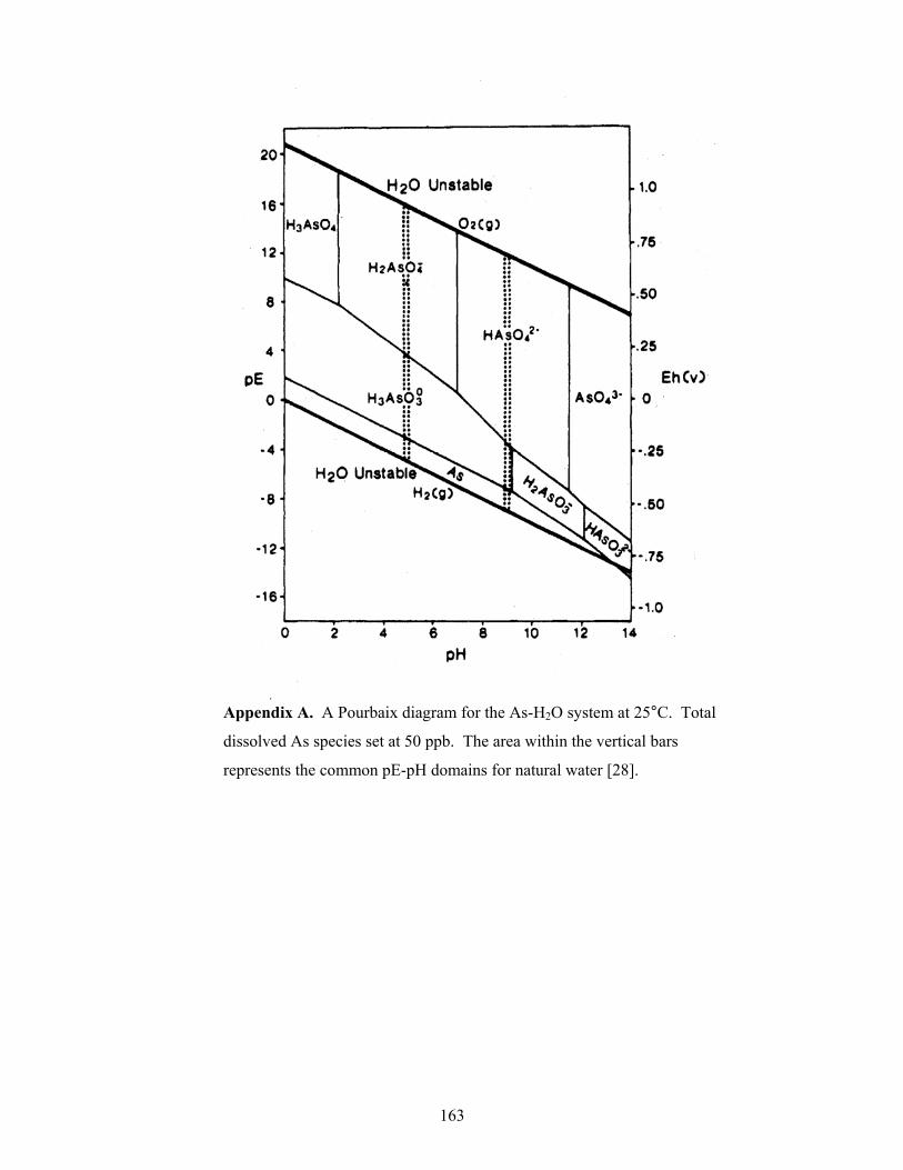
163
Appendix A. A Pourbaix diagram for the As-H2O system at 25°C. Total
dissolved As species set at 50 ppb. The area within the vertical bars
represents the common pE-pH domains for natural water [28].

164
APPENDIX B
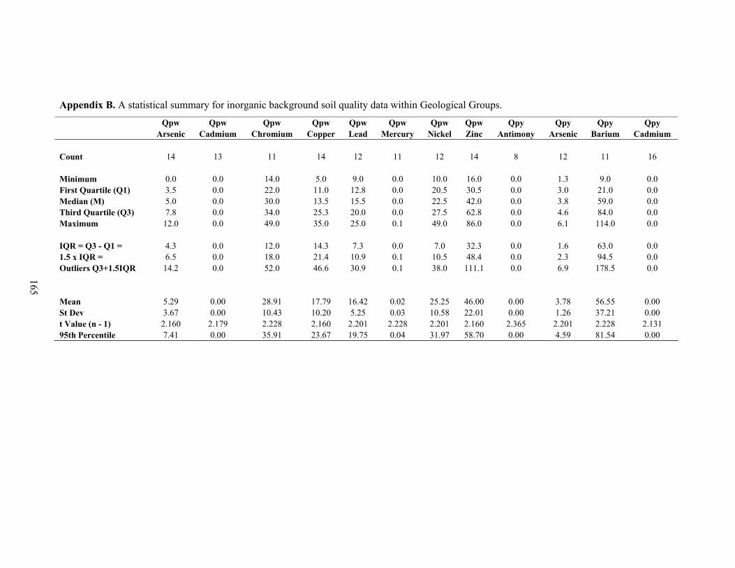
165
Appendix B. A statistical summary for inorganic background soil quality data within Geological Groups.
Qpw Qpw Qpw Qpw Qpw Qpw Qpw Qpw Qpy Qpy Qpy Qpy Arsenic Cadmium Chromium Copper Lead Mercury Nickel Zinc Antimony Arsenic Barium Cadmium
Count 14 13 11 14 12 11 12 14 8 12 11 16 Minimum 0.0 0.0 14.0 5.0 9.0 0.0 10.0 16.0 0.0 1.3 9.0 0.0 First Quartile (Q1) 3.5 0.0 22.0 11.0 12.8 0.0 20.5 30.5 0.0 3.0 21.0 0.0 Median (M) 5.0 0.0 30.0 13.5 15.5 0.0 22.5 42.0 0.0 3.8 59.0 0.0 Third Quartile (Q3) 7.8 0.0 34.0 25.3 20.0 0.0 27.5 62.8 0.0 4.6 84.0 0.0 Maximum 12.0 0.0 49.0 35.0 25.0 0.1 49.0 86.0 0.0 6.1 114.0 0.0 IQR = Q3 - Q1 = 4.3 0.0 12.0 14.3 7.3 0.0 7.0 32.3 0.0 1.6 63.0 0.0 1.5 x IQR = 6.5 0.0 18.0 21.4 10.9 0.1 10.5 48.4 0.0 2.3 94.5 0.0 Outliers Q3+1.5IQR 14.2 0.0 52.0 46.6 30.9 0.1 38.0 111.1 0.0 6.9 178.5 0.0 Mean 5.29 0.00 28.91 17.79 16.42 0.02 25.25 46.00 0.00 3.78 56.55 0.00 St Dev 3.67 0.00 10.43 10.20 5.25 0.03 10.58 22.01 0.00 1.26 37.21 0.00 t Value (n - 1) 2.160 2.179 2.228 2.160 2.201 2.228 2.201 2.160 2.365 2.201 2.228 2.131 95th Percentile 7.41 0.00 35.91 23.67 19.75 0.04 31.97 58.70 0.00 4.59 81.54 0.00

166
Appendix B (Cont…). A statistical summary for inorganic background soil quality data within Geological Groups.
Qpy Qpy Qpy Qpy Qpy Qpy Qpy Qpy Qrc Qrc Qrc Qrc Qrc Chromium Copper Lead Mercury Nickel Soil pH Tin Zinc Arsenic Cadmium Chromium Copper Lead
Count 20 20 19 16 18 9 9 16 11 11 9 11 10 Minimum 5.9 0.0 2.0 0.0 4.0 3.2 0.0 3.0 0.0 0.0 32.0 7.4 0.0 First Quartile (Q1) 18.0 6.5 6.5 0.0 22.3 6.4 0.0 16.8 0.0 0.0 46.0 13.5 5.0 Median (M) 31.0 9.0 10.0 0.0 27.5 7.7 0.0 31.5 0.0 0.0 51.0 18.0 6.3 Third Quartile (Q3) 49.3 14.5 15.0 0.0 37.3 8.3 0.0 37.0 3.8 0.0 55.0 22.0 8.8 Maximum 66.0 26.0 30.0 0.1 42.0 9.3 0.0 66.0 9.0 0.0 66.0 32.0 15.0 IQR = Q3 - Q1 = 31.3 8.1 8.5 0.0 15.0 1.9 0.0 20.3 3.8 0.0 9.0 8.5 3.8 1.5 x IQR = 46.9 12.1 12.8 0.0 22.5 2.9 0.0 30.4 5.6 0.0 13.5 12.8 5.6 Outliers Q3+1.5IQR 96.1 26.6 27.8 0.1 59.8 11.2 0.0 67.4 9.4 0.0 68.5 34.8 14.4 Mean 33.94 11.18 12.66 0.02 28.06 7.08 0.00 28.94 2.22 0.00 50.89 18.04 6.79 St Dev 19.92 7.01 8.17 0.03 11.22 1.89 0.00 16.83 2.98 0.00 9.73 7.02 4.29 t Value (n - 1) 2.093 2.093 2.101 2.131 2.110 2.306 2.306 2.131 2.228 2.228 2.306 2.228 2.262 95th Percentile 43.26 14.46 16.60 0.03 33.63 8.53 0.00 37.90 4.22 0.00 58.37 22.75 9.86
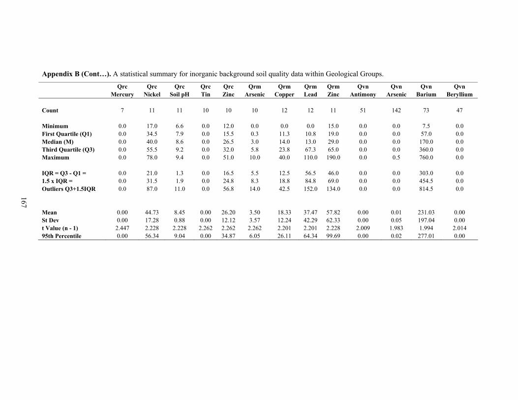
167
Appendix B (Cont…). A statistical summary for inorganic background soil quality data within Geological Groups.
Qrc Qrc Qrc Qrc Qrc Qrm Qrm Qrm Qrm Qvn Qvn Qvn Qvn Mercury Nickel Soil pH Tin Zinc Arsenic Copper Lead Zinc Antimony Arsenic Barium Beryllium
Count 7 11 11 10 10 10 12 12 11 51 142 73 47 Minimum 0.0 17.0 6.6 0.0 12.0 0.0 0.0 0.0 15.0 0.0 0.0 7.5 0.0 First Quartile (Q1) 0.0 34.5 7.9 0.0 15.5 0.3 11.3 10.8 19.0 0.0 0.0 57.0 0.0 Median (M) 0.0 40.0 8.6 0.0 26.5 3.0 14.0 13.0 29.0 0.0 0.0 170.0 0.0 Third Quartile (Q3) 0.0 55.5 9.2 0.0 32.0 5.8 23.8 67.3 65.0 0.0 0.0 360.0 0.0 Maximum 0.0 78.0 9.4 0.0 51.0 10.0 40.0 110.0 190.0 0.0 0.5 760.0 0.0 IQR = Q3 - Q1 = 0.0 21.0 1.3 0.0 16.5 5.5 12.5 56.5 46.0 0.0 0.0 303.0 0.0 1.5 x IQR = 0.0 31.5 1.9 0.0 24.8 8.3 18.8 84.8 69.0 0.0 0.0 454.5 0.0 Outliers Q3+1.5IQR 0.0 87.0 11.0 0.0 56.8 14.0 42.5 152.0 134.0 0.0 0.0 814.5 0.0 Mean 0.00 44.73 8.45 0.00 26.20 3.50 18.33 37.47 57.82 0.00 0.01 231.03 0.00 St Dev 0.00 17.28 0.88 0.00 12.12 3.57 12.24 42.29 62.33 0.00 0.05 197.04 0.00 t Value (n - 1) 2.447 2.228 2.228 2.262 2.262 2.262 2.201 2.201 2.228 2.009 1.983 1.994 2.014 95th Percentile 0.00 56.34 9.04 0.00 34.87 6.05 26.11 64.34 99.69 0.00 0.02 277.01 0.00

168
Appendix B (Cont…). A statistical summary for inorganic background soil quality data within Geological Groups.
Qvn Qvn Qvn Qvn Qvn Qvn Qvn Qvn Qvn Qvn Qvn Boron Cadmium Chromium Cobalt Copper Lead Manganese Mercury Molybdenum Nickel Selenium
Count 13 185 191 105 200 189 15 117 43 174 54 Minimum 0.0 0.0 7.3 0.0 0.0 0.0 0.0 0.0 0.0 0.0 0.0 First Quartile (Q1) 0.0 0.0 24.5 11.0 7.7 7.4 122.0 0.0 0.0 14.0 0.0 Median (M) 0.0 0.0 34.0 16.0 11.0 11.0 260.0 0.0 0.0 21.0 0.0 Third Quartile (Q3) 8.0 0.0 42.5 20.0 16.0 15.0 405.0 0.0 0.0 32.0 0.0 Maximum 19.0 0.0 73.0 30.0 28.0 28.0 560.0 0.0 0.0 62.0 0.0 IQR = Q3 - Q1 = 8.0 0.0 18.0 9.0 8.3 7.6 283.0 0.0 0.0 18.0 0.0 1.5 x IQR = 12.0 0.0 27.0 13.5 12.5 11.4 424.5 0.0 0.0 27.0 0.0 Outliers Q3+1.5IQR 20.0 0.0 69.5 33.5 28.5 26.4 829.5 0.0 0.0 59.0 0.0 Mean 4.19 0.00 35.02 15.26 11.75 11.35 260.67 0.00 0.00 23.24 0.00 St Dev 6.92 0.00 14.47 6.69 6.17 6.34 190.67 0.00 0.00 12.91 0.00 t Value (n - 1) 2.179 1.982 1.982 1.984 1.982 1.982 2.145 1.984 2.019 1.982 2.006 95th Percentile 8.37 0.00 37.09 16.55 12.61 12.26 366.27 0.00 0.00 25.18 0.00
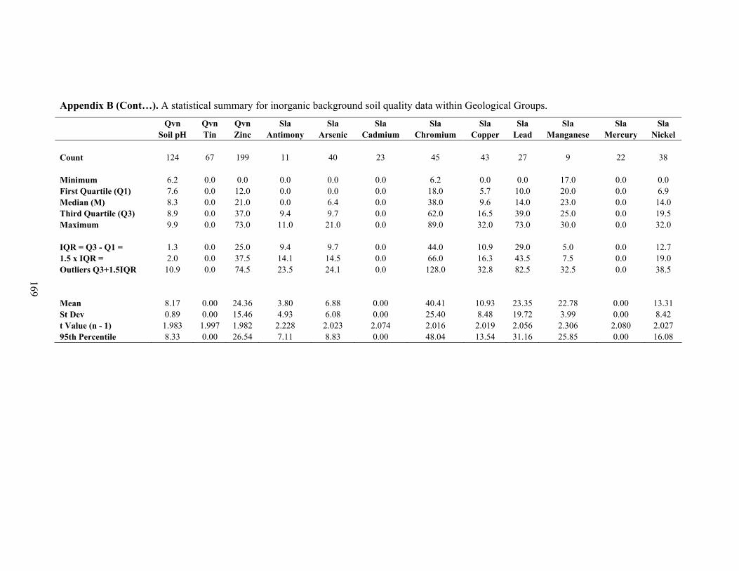
169
Appendix B (Cont…). A statistical summary for inorganic background soil quality data within Geological Groups.
Qvn Qvn Qvn Sla Sla Sla Sla Sla Sla Sla Sla Sla Soil pH Tin Zinc Antimony Arsenic Cadmium Chromium Copper Lead Manganese Mercury Nickel
Count 124 67 199 11 40 23 45 43 27 9 22 38 Minimum 6.2 0.0 0.0 0.0 0.0 0.0 6.2 0.0 0.0 17.0 0.0 0.0 First Quartile (Q1) 7.6 0.0 12.0 0.0 0.0 0.0 18.0 5.7 10.0 20.0 0.0 6.9 Median (M) 8.3 0.0 21.0 0.0 6.4 0.0 38.0 9.6 14.0 23.0 0.0 14.0 Third Quartile (Q3) 8.9 0.0 37.0 9.4 9.7 0.0 62.0 16.5 39.0 25.0 0.0 19.5 Maximum 9.9 0.0 73.0 11.0 21.0 0.0 89.0 32.0 73.0 30.0 0.0 32.0 IQR = Q3 - Q1 = 1.3 0.0 25.0 9.4 9.7 0.0 44.0 10.9 29.0 5.0 0.0 12.7 1.5 x IQR = 2.0 0.0 37.5 14.1 14.5 0.0 66.0 16.3 43.5 7.5 0.0 19.0 Outliers Q3+1.5IQR 10.9 0.0 74.5 23.5 24.1 0.0 128.0 32.8 82.5 32.5 0.0 38.5 Mean 8.17 0.00 24.36 3.80 6.88 0.00 40.41 10.93 23.35 22.78 0.00 13.31 St Dev 0.89 0.00 15.46 4.93 6.08 0.00 25.40 8.48 19.72 3.99 0.00 8.42 t Value (n - 1) 1.983 1.997 1.982 2.228 2.023 2.074 2.016 2.019 2.056 2.306 2.080 2.027 95th Percentile 8.33 0.00 26.54 7.11 8.83 0.00 48.04 13.54 31.16 25.85 0.00 16.08
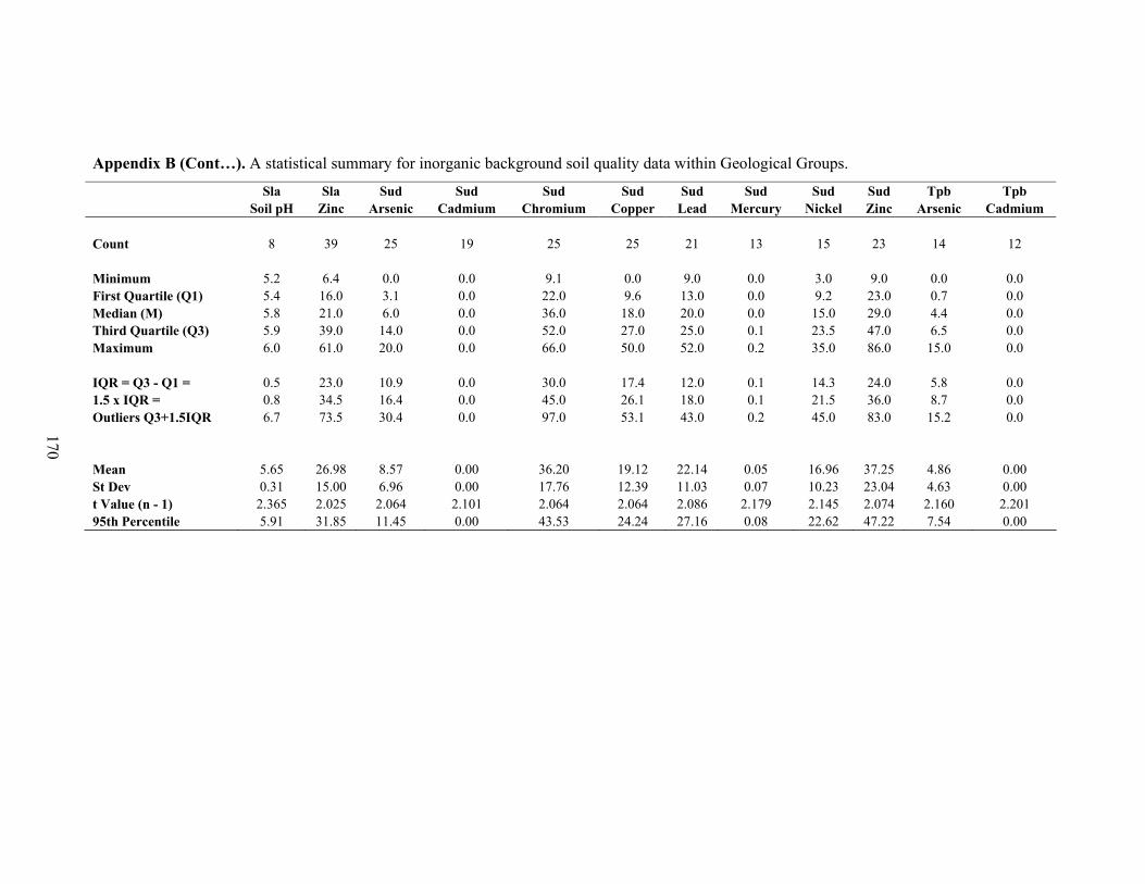
170
Appendix B (Cont…). A statistical summary for inorganic background soil quality data within Geological Groups.
Sla Sla Sud Sud Sud Sud Sud Sud Sud Sud Tpb Tpb Soil pH Zinc Arsenic Cadmium Chromium Copper Lead Mercury Nickel Zinc Arsenic Cadmium
Count 8 39 25 19 25 25 21 13 15 23 14 12 Minimum 5.2 6.4 0.0 0.0 9.1 0.0 9.0 0.0 3.0 9.0 0.0 0.0 First Quartile (Q1) 5.4 16.0 3.1 0.0 22.0 9.6 13.0 0.0 9.2 23.0 0.7 0.0 Median (M) 5.8 21.0 6.0 0.0 36.0 18.0 20.0 0.0 15.0 29.0 4.4 0.0 Third Quartile (Q3) 5.9 39.0 14.0 0.0 52.0 27.0 25.0 0.1 23.5 47.0 6.5 0.0 Maximum 6.0 61.0 20.0 0.0 66.0 50.0 52.0 0.2 35.0 86.0 15.0 0.0 IQR = Q3 - Q1 = 0.5 23.0 10.9 0.0 30.0 17.4 12.0 0.1 14.3 24.0 5.8 0.0 1.5 x IQR = 0.8 34.5 16.4 0.0 45.0 26.1 18.0 0.1 21.5 36.0 8.7 0.0 Outliers Q3+1.5IQR 6.7 73.5 30.4 0.0 97.0 53.1 43.0 0.2 45.0 83.0 15.2 0.0 Mean 5.65 26.98 8.57 0.00 36.20 19.12 22.14 0.05 16.96 37.25 4.86 0.00 St Dev 0.31 15.00 6.96 0.00 17.76 12.39 11.03 0.07 10.23 23.04 4.63 0.00 t Value (n - 1) 2.365 2.025 2.064 2.101 2.064 2.064 2.086 2.179 2.145 2.074 2.160 2.201 95th Percentile 5.91 31.85 11.45 0.00 43.53 24.24 27.16 0.08 22.62 47.22 7.54 0.00

171
Appendix B (Cont…). A statistical summary for inorganic background soil quality data within Geological Groups.
Tpb Tpb Tpb Tpb Tpb Tpb Tvo Tvo Tvo Tvo Tvo Tvo Chromium Copper Lead Mercury Nickel Zinc Arsenic Chromium Copper Mercury Nickel Zinc
Count 16 14 13 10 10 12 7 7 8 8 8 6 Minimum 0.0 0.0 0.0 0.0 0.0 12.0 0.0 30.0 0.0 0.0 24.0 15.0 First Quartile (Q1) 8.8 1.5 10.0 0.0 8.1 17.5 2.4 34.0 0.0 0.0 31.3 16.5 Median (M) 31.0 9.4 12.0 0.0 12.7 37.0 2.6 40.0 3.0 0.0 34.0 19.0 Third Quartile (Q3) 38.0 17.8 55.0 0.1 24.8 61.5 2.8 40.0 13.4 0.0 39.0 23.0 Maximum 56.0 32.0 93.0 0.2 43.0 110.0 4.0 59.0 28.0 0.0 42.0 26.0 IQR = Q3 - Q1 = 29.2 16.2 45.0 0.1 16.7 44.0 0.5 6.0 13.4 0.0 7.8 6.5 1.5 x IQR = 43.8 24.3 67.5 0.2 25.1 66.0 0.7 9.0 20.1 0.0 11.6 9.8 Outliers Q3+1.5IQR 81.8 42.1 122.5 0.3 49.8 127.5 3.5 49.0 33.5 0.0 50.6 32.8 Mean 25.99 10.74 30.54 0.06 17.01 46.25 2.41 39.57 8.64 0.00 34.13 19.83 St Dev 17.44 9.62 31.56 0.07 13.29 35.61 1.21 9.43 11.85 0.00 6.66 4.40 t Value (n - 1) 2.131 2.160 2.179 2.262 2.262 2.201 2.447 2.447 2.365 2.365 2.365 2.571 95th Percentile 35.28 16.29 49.61 0.11 26.52 68.88 3.53 48.29 18.54 0.00 39.70 24.45
Notes: Qpw (also called Qpd) – Quaternary, Pleistocene: Description: Aeolian: Dune deposits: sand, clay, calcareous sand; Qpy - Quaternary, Pleistocene (Coode Island Silt): Paludal: lagoon deposits: black silt, clay; Qrc – Quaternary, Mostly Holocene: Fluvial: “gully” alluvium, colluvium: gravel, sand, silt; Qrm – Quaternary, Mostly Holocene: Paludal: lagoon and swamp deposits: silt, clay; Qvn – Quaternary/Tertiary, Holocene to Pliocene (Newer Volcanics): Extrusive: tholeiitic to alkaline basalts, minor scoria and ash; Sla – Silurian, Lower (Anderson Creek Formation): Marine: sandstone, thick to thin bedded, siltstone, minor conglomerate; Sud – Silurian, Upper (Dargile Formation): Marine: siltstone, thick bedded, sandstone; Tpb – Tertiary, Pliocene to Miocene (Brighton Group): Fluvial: gravel, sand, silt; Tvo – Tertiary, Eocene to Oligocene (Older Volcanics): Extrusive: tholeiitic and minor alkaline basalts.

172
APPENDIX C
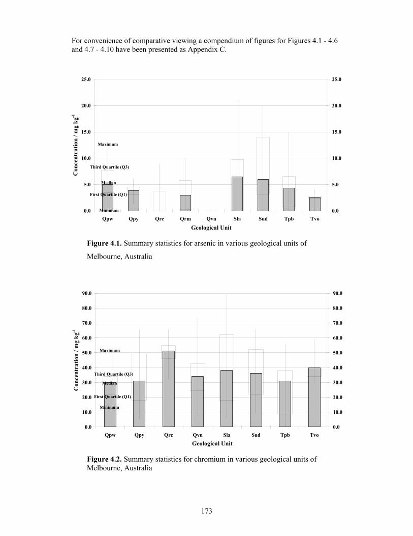
173
For convenience of comparative viewing a compendium of figures for Figures 4.1 - 4.6 and 4.7 - 4.10 have been presented as Appendix C.
0.0
5.0
10.0
15.0
20.0
25.0
Qpw Qpy Qrc Qrm Qvn Sla Sud Tpb Tvo
Geological Unit
Con
cent
ratio
n / m
g kg
-1
0.0
5.0
10.0
15.0
20.0
25.0
Maximum
Minimum
First Quartile (Q1)
Third Quartile (Q3)
Median
Figure 4.1. Summary statistics for arsenic in various geological units of
Melbourne, Australia
0.0
10.0
20.0
30.0
40.0
50.0
60.0
70.0
80.0
90.0
Qpw Qpy Qrc Qvn Sla Sud Tpb TvoGeological Unit
Con
cent
ratio
n / m
g kg
-1
0.0
10.0
20.0
30.0
40.0
50.0
60.0
70.0
80.0
90.0
Maximum
Third Quartile (Q3)
Median
First Quartile (Q1)
Minimum
Figure 4.2. Summary statistics for chromium in various geological units of Melbourne, Australia
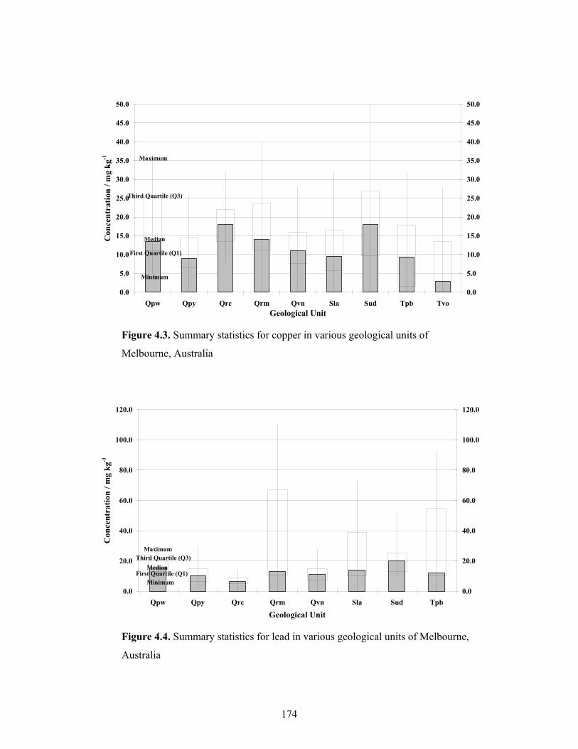
174
0.0
5.0
10.0
15.0
20.0
25.0
30.0
35.0
40.0
45.0
50.0
Qpw Qpy Qrc Qrm Qvn Sla Sud Tpb TvoGeological Unit
Con
cent
ratio
n / m
g kg
-1
0.0
5.0
10.0
15.0
20.0
25.0
30.0
35.0
40.0
45.0
50.0
Maximum
Third Quartile (Q3)
Median
First Quartile (Q1)
Minimum
Figure 4.3. Summary statistics for copper in various geological units of
Melbourne, Australia
0.0
20.0
40.0
60.0
80.0
100.0
120.0
Qpw Qpy Qrc Qrm Qvn Sla Sud Tpb
Geological Unit
Con
cent
ratio
n / m
g kg
-1
0.0
20.0
40.0
60.0
80.0
100.0
120.0
MaximumThird Quartile (Q3)
MedianFirst Quartile (Q1)
Minimum
Figure 4.4. Summary statistics for lead in various geological units of Melbourne,
Australia
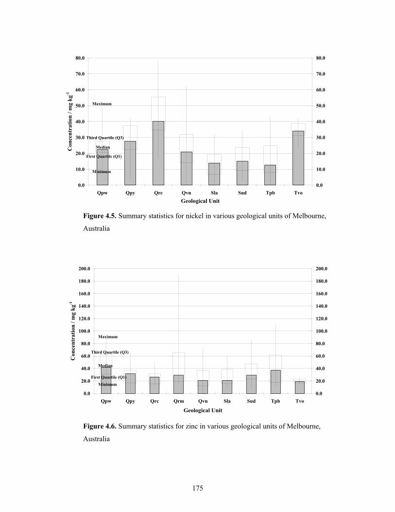
175
0.0
10.0
20.0
30.0
40.0
50.0
60.0
70.0
80.0
Qpw Qpy Qrc Qvn Sla Sud Tpb TvoGeological Unit
Con
cent
ratio
n / m
g kg
-1
0.0
10.0
20.0
30.0
40.0
50.0
60.0
70.0
80.0
Maximum
Third Quartile (Q3)
Median
First Quartile (Q1)
Minimum
Figure 4.5. Summary statistics for nickel in various geological units of Melbourne,
Australia
0.0
20.0
40.0
60.0
80.0
100.0
120.0
140.0
160.0
180.0
200.0
Qpw Qpy Qrc Qrm Qvn Sla Sud Tpb Tvo
Geological Unit
Con
cent
ratio
n / m
g kg
-1
0.0
20.0
40.0
60.0
80.0
100.0
120.0
140.0
160.0
180.0
200.0
Maximum
Third Quartile (Q3)
Median
First Quartile (Q1)Minimum
Figure 4.6. Summary statistics for zinc in various geological units of Melbourne,
Australia
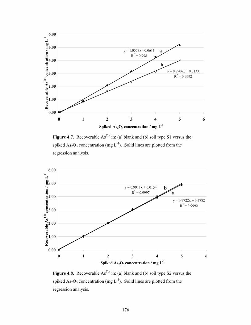
176
y = 1.0573x - 0.0611R2 = 0.998
y = 0.7906x + 0.0133R2 = 0.9992
0.00
1.00
2.00
3.00
4.00
5.00
6.00
0 1 2 3 4 5 6Spiked As2O3 concentration / mg L-1
Rec
over
able
AsT
ot c
once
ntra
tion
/ mg
L-1
a
b
Figure 4.7. Recoverable AsTot in: (a) blank and (b) soil type S1 versus the
spiked As2O3 concentration (mg L-1). Solid lines are plotted from the
regression analysis.
y = 0.9722x + 0.5782R2 = 0.9992
y = 0.9911x + 0.0154R2 = 0.9997
0.00
1.00
2.00
3.00
4.00
5.00
6.00
0 1 2 3 4 5 6
Spiked As2O3 concentration / mg L-1
Rec
over
able
AsT
ot c
once
ntra
tion
/ mg
L-1
ab
Figure 4.8. Recoverable AsTot in: (a) blank and (b) soil type S2 versus the
spiked As2O3 concentration (mg L-1). Solid lines are plotted from the
regression analysis.
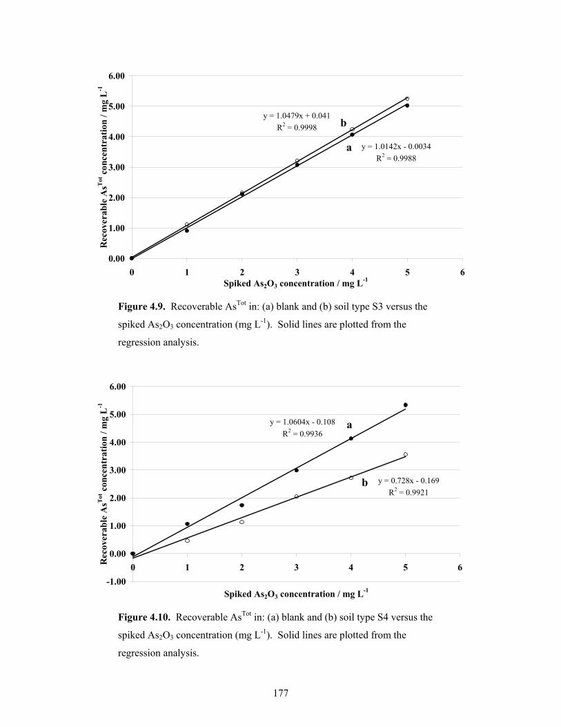
177
y = 1.0142x - 0.0034R2 = 0.9988
y = 1.0479x + 0.041R2 = 0.9998
0.00
1.00
2.00
3.00
4.00
5.00
6.00
0 1 2 3 4 5 6Spiked As2O3 concentration / mg L-1
Rec
over
able
AsT
ot c
once
ntra
tion
/ mg
L-1
a
b
Figure 4.9. Recoverable AsTot in: (a) blank and (b) soil type S3 versus the
spiked As2O3 concentration (mg L-1). Solid lines are plotted from the
regression analysis.
y = 1.0604x - 0.108R2 = 0.9936
y = 0.728x - 0.169R2 = 0.9921
-1.00
0.00
1.00
2.00
3.00
4.00
5.00
6.00
0 1 2 3 4 5 6
Spiked As2O3 concentration / mg L-1
Rec
over
able
AsT
ot c
once
ntra
tion
/ mg
L-1
a
b
Figure 4.10. Recoverable AsTot in: (a) blank and (b) soil type S4 versus the
spiked As2O3 concentration (mg L-1). Solid lines are plotted from the
regression analysis.