Analog Circuits and Systems Prof. K Radhakrishna Rao

Lecture 25: Active Filters

1

Review

�  Inductor Simulation �  To convert RLC filters to Active RC filters �  Gyrator – Inductor Simulator (L=CR2) �  Active and Passive - Parameter Sensitivities in Active RC filters �  Effect of finite gain and finite gain bandwidth product on inductor

simulated �  f0Q<<Gain Bandwidth Product

2

Review (contd.,)

3

of the inductor simulated =

of the filter simulated =

0

0 0

a

a 0 a

0

AQ2 A1GBQQ

Q 2 Q1A GB

ω⎛ ⎞−⎜ ⎟⎝ ⎠

⎛ ⎞ω+ −⎜ ⎟⎝ ⎠

Q-enhancement- Sallen and Key

�  The quality factor Qp of a second order passive RC filter is always less than 0.5

�  Qp < 0.5 is unacceptable for a general filter design �  Sallen and Key proposed use of negative and positive feedback, and

active devices to enhance Q �  Several topologies similar to Sallen and Key filters are possible

4

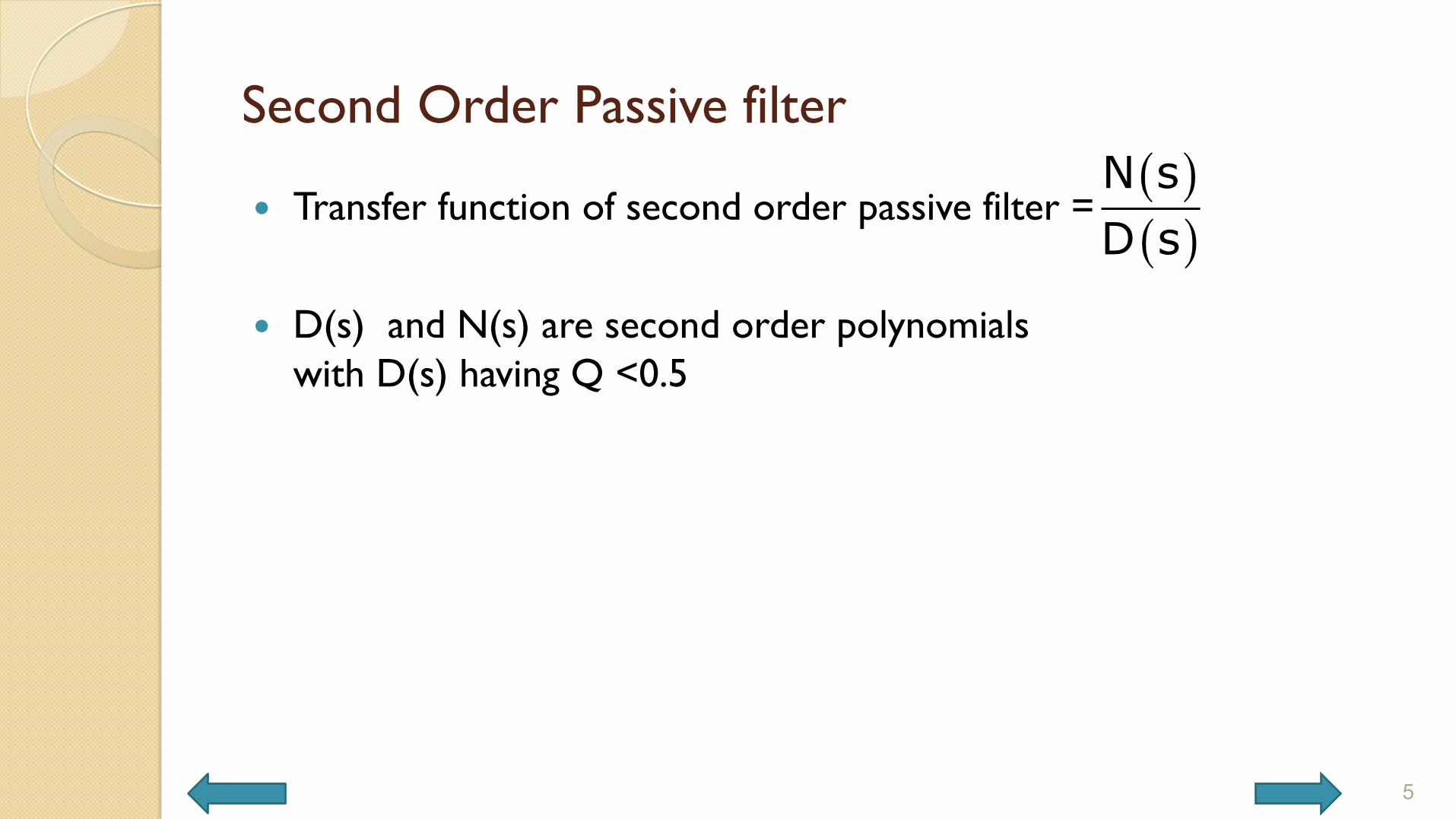
Second Order Passive filter

�  Transfer function of second order passive filter =

�  D(s) and N(s) are second order polynomials with D(s) having Q <0.5

5

( )( )N sD s

Use of feedback to enhance Q

6

( ) ( )( ) ( )

( )( ) ( )

o

i

-K N s D s -KN sVV D s KN s1 K N s D s

⎡ ⎤⎣ ⎦= =+⎡ ⎤+ ⎣ ⎦

where K is the gain of the active device

Use of feedback to enhance Q (contd.,)

7

p

For a general second-order passive RC/RL filter

where is the natural frequency of the passive RC filter

is quality factor of the passive second-order RC/RL

2

2pp

2

2p pp

p

s sm n pN(s)D(s) s s 1

Q

Q

⎡ ⎤+ +⎢ ⎥ωω⎢ ⎥⎣ ⎦=

⎡ ⎤+ +⎢ ⎥ωω⎢ ⎥⎣ ⎦

ω

filter

Quality Factor

8

is always < 0.5p

2

2p po

2i

2p p p

0 p

pa

Q

s s-K m n pVV s s(1 mK) (1 nK) (1 pK)

Q

1 pK1 mKQ

Q (1 pK) (1 mK)(1 nK)

⎡ ⎤+ +⎢ ⎥ω ω⎢ ⎥⎣ ⎦=

⎡ ⎤+ + + + +⎢ ⎥ω ω⎢ ⎥⎣ ⎦+ω = ω+

= + ++

If K is positive, m and p are positive, and for all values of n it is a negative feedback system If K is negative m and p are positive, all positive values of n it is a positive feedback system

Enhancement of Qa

�  Qa can be enhanced by increasing pK >0 with m = n =0, mK>0 with p=n=0, pK>0 and mK>0 with n =0. These make use of negative feedback.

�  Qa can also be enhanced by making nK<0 and 0<|nK|<1. This constitutes using positive feedback.

�  All types of filters can be designed using any of the Q-enhancement methods.

9

Second-order low-pass RC filter

10

with and

and

p1 1 2 2

p1 1 2 2 1

2 2 1 1 2

1 2 1 2

p p

1R C R C

1QC R C R R1C R C R R

R R R C C C1 1QRC 3

ω =

=⎛ ⎞

+ +⎜ ⎟⎝ ⎠

= = = =

ω = =

( ) ( )( )21 1 2 2 1 1 2 1 2

N(s) 1D(s) C R C R s C R C R R s 1

=+ + + +

Active Low Pass Filter

11

The natural frequency of the active filter is now higher

can be increased to the required value through

suitable selection of .Low-

o2

i2

p pp

0 p a p

a

m 0, n 0 and p 1V -KV s s (1 K)

Q

1 K ; Q Q 1 KQ

K

= = =

=⎡ ⎤

+ + +⎢ ⎥ωω⎢ ⎥⎣ ⎦

ω = ω + = +

pass passive filter with amplifier gain - and feedbackK

and 1 2 1 2R R R C C C= = = =

Structure of Active Low Pass filter

�  Addition required between feedback signal and the input �  In order to get 2Vo the gain of VCVS will have to be made 2K �  A VCVS with gain -K can be realized by having buffer stage

followed by inverting amplifier

12

Structure of Active Low Pass filter (contd.,)

13

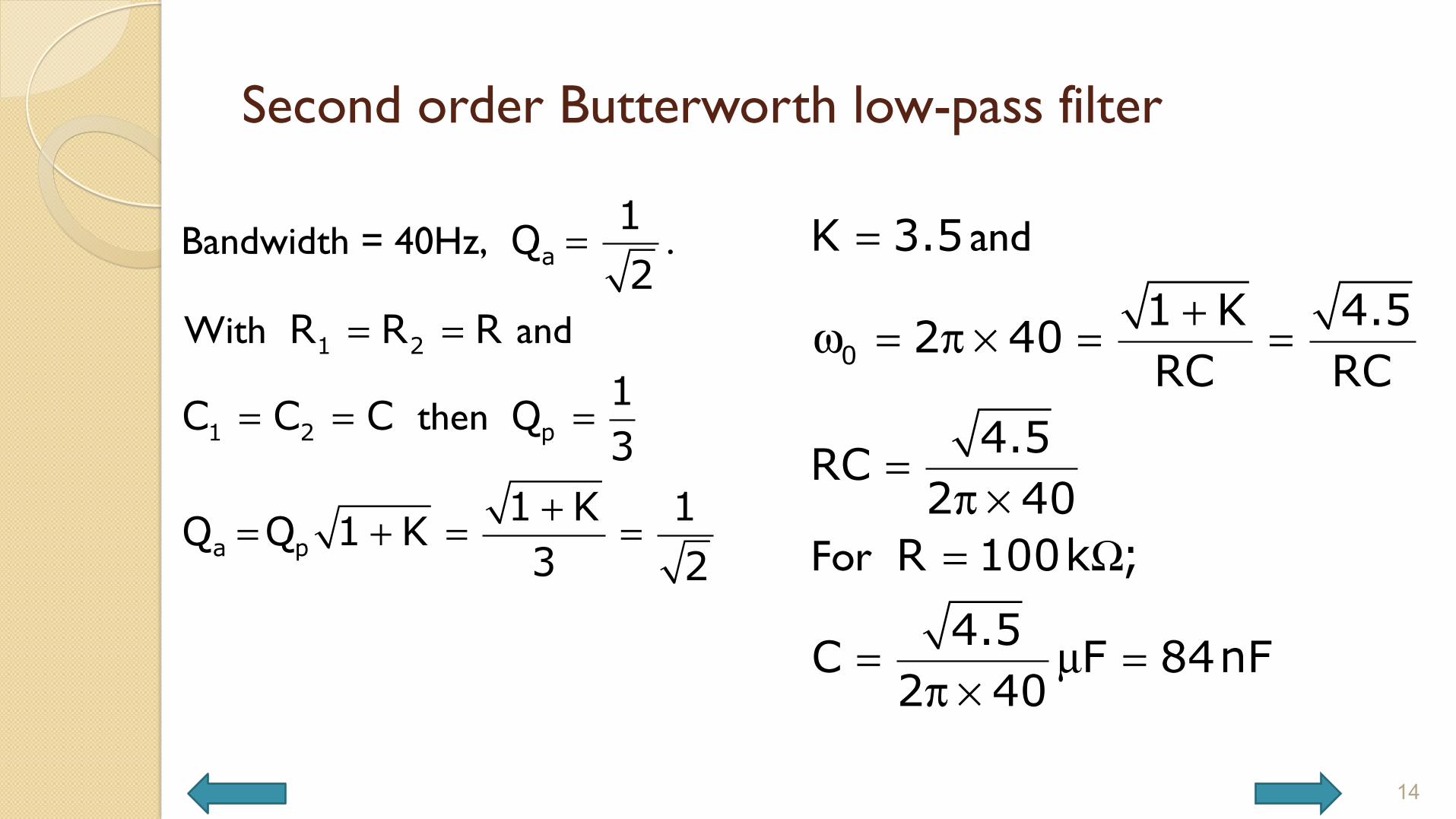
Second order Butterworth low-pass filter

14

Bandwidth = 40Hz, .

With and

then

a

1 2

1 2 p

a p

1Q2

R R R1C C C Q3

1 K 1Q Q 1 K3 2

=

= =

= = =

+= + = =

and

For

0

K 3.5

1 K 4.52 40RC RC

4.5RC2 40R 100k ;

4.5C F 84nF2 40

=

+ω = π × = =

=π ×= Ω

= µ =π ×

Frequency Response of the Butterworth LP filter

15

Transient Response of the Butterworth LP filter

16

Frequency response of Low Pass Filter

17

with Q =5 and f0 = 40 Hz R=100k; C=0.6mF; K=224

Frequency response of Low Pass Filter

18

with Q =5 and f0 = 400 Hz C = 60 nF Finite GB of the Op.Amp

Finite GB of the Op.Amp

Transient response of Low-pass Filter

19

with Q =5 and f0 = 400 Hz C = 60 nF

Q-Enhancement due to Finite GB

Low-pass Filter

20

with Q =5 and f0 = 600 Hz C = 40 nF

Q-Enhancement due to Finite GB

Observations

�  Q increases from the specified value �  The natural frequency reduces slightly from the specified value �  At higher natural frequencies the transient responses are more

oscillatory indicating Q enhancement �  Beyond a certain natural frequency the system becomes unstable

and goes into oscillations at the natural frequency �  These deviations from the expected behavior are due to finite gain

bandwidth product of the active devices used.

21

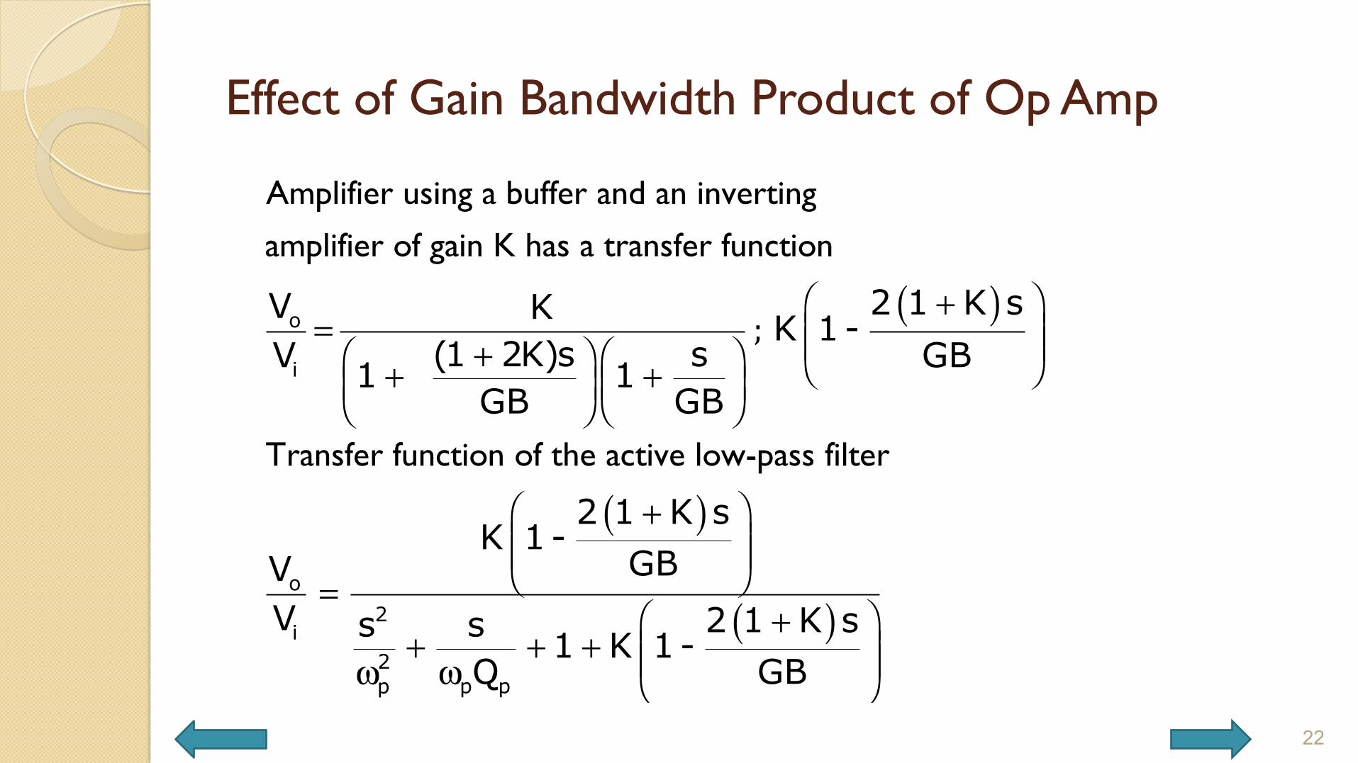
Effect of Gain Bandwidth Product of Op Amp

( )

( )

⎛ ⎞+= ⎜ ⎟⎜ ⎟+⎛ ⎞ ⎛ ⎞ ⎝ ⎠+ +⎜ ⎟ ⎜ ⎟⎝ ⎠ ⎝ ⎠

+

=

Amplifier using a buffer and an inverting

amplifier of gain K has a transfer function

Transfer function of the active low-pass filter

o

i

o

i

2 1 K sV K K 1-(1 2K)s sV GB1 1GB GB

2 1 K sK 1-

GVV

;

( )

⎛ ⎞⎜ ⎟⎜ ⎟⎝ ⎠

⎛ ⎞++ + + ⎜ ⎟⎜ ⎟ωω ⎝ ⎠

2

2p pp

B2 1 K ss s 1 K 1-

Q GB

22

Effect of GB Product of Op Amp (contd.,)

( )

( )

( )

Normalizing

(due to GB)

o2

i20 0 p

pa

0 p

2 1 K sK 1-1 K GBV

V 2K 1 K ss s - 1GB(1 K)Q 1 K

Q 1 KQ

2K 1 K Q1-

1 KGB

⎛ ⎞+⎜ ⎟⎜ ⎟+ ⎝ ⎠=

⎛ ⎞++ +⎜ ⎟⎜ ⎟+ω ω + ⎝ ⎠

+=⎛ ⎞+ ω⎜ ⎟⎜ ⎟+⎝ ⎠

23

( )GB should be large enough

to make 0 p

0 a

2K 1 K Q1 KGB

2K Q 1GB

+ ω

+ω

= =

Examples

24

Ex:1

(specified) and Hz and

(due to GB)

a 0

pa

0 a

Q 5 f 40 K 3.5

Q 1 KQ 5.23

2K Q1-GB

= = =

+= =

ω⎛ ⎞⎜ ⎟⎝ ⎠

Ex:2

(specified)=5 and Hz and

(due to GB)

a 0

pa

0 a

Q f 400 K 224

Q 1 KQ 48

2K Q1-GB

= =

+= =

ω⎛ ⎞⎜ ⎟⎝ ⎠

Limitations of GB

for the filter to be stable in case inductance simulation

for the filter to be stable in case of filter using feedback

0 a

0 a

2f Q 1GB

2Kf Q 1GB

=

=

25

Fourth-order Butterworth Low-pass Filter

26

2 2

2 20 00 0

1s s s s1 0.765 1 1.848

⎡ ⎤ ⎡ ⎤+ + + +⎢ ⎥ ⎢ ⎥ω ωω ω⎢ ⎥ ⎢ ⎥⎣ ⎦ ⎣ ⎦

Effect of finite GB

27

�  Taking GB into account with f0 = 3.3 kHz (speech filter)

�  Using 741 Op Amp having a GB of 1 MHz

�  Q of the 2nd second-order filter changes by 1%

�  Q of the first second-order filter changes by about 12.4%

High Pass Filter

28

( )

( )

and p

Natural frequency of the

active filter

2

2po

2i

2p pp

p0

m 1, n 0 0s-K

VV s s1 K 1

Q

1 K

= = =

ω=⎡ ⎤

+ + +⎢ ⎥ωω⎢ ⎥⎣ ⎦

ωω =

+

Natural frequency of the

active filter decreases by

a factor

The quality factor of the

active filter can be increased

to the required value through

suitable selection of

a p

1 K

Q Q 1 KQ

K.

+

= +

Passive HP filter

29

Active HP filter

30

Active HP Filter (contd.,)

31

( )

( ) ( )( ) ( )( )

where and

Required is obtained by selecting .

is determined for a specified and

2

2 2 po 0p 02

i 1 1 2 22

00

a p

1 1 2 2 2 2 1 1 1 2

a

p 0

s-KV 1 ;V C R C Rs s 1 K1

Q

1 KQ Q 1 KC R C R C R C R 1 R R

Q KK.

ωω= ω = ω =

++ +ωω

+= = ++ +

ω ω

Topology of active HP filter

32

Example If the lower cut off frequency is selected as 0.4 Hz.

Assuming and

for maximally flat response

For

1 2 1 2 p

a

a p

0

1C C C R R R; Q3

1Q2

1 K 1Q Q 1 K ;K 3.53 21 1 12 0.4 ;RC

RC 1 K RC 4.5 2 0.4 4.51R 100k ;C

0.8

= = = = =

=

+= + = = =

ω = π × = = =+ π ×

= Ω =π

1.8 F4.5

= µ

33

Simulation

34

Single Op Amp Topology

�  Buffer amplifier can be removed by suitable adjustment of the resistances

35

R1 = R = R3//R4 and C1 = C2 = C

Q of active filters

36

( )

of the circuit gets enhanced by a factor of

in case of low-pass and high-pass active filters

Natural frequency of the active low-pass filter

Natural frequency of the active high-pass filt

0 p

Q 1 K

1 K

+

ω = + ω

( )er p0

1 K

ωω =

+

Effect of finite GB

�  High Pass filter with f0 = 400 Hz and Q = 5 �  Q = 5 gives K = 224 �  For f0=400 Hz and R = 100 kW gives C = 265 pF

37

Effect of finite GB (contd.,)

( )

( )

( )

( )

⎡ ⎤+⇒ ⎢ ⎥

⎢ ⎥⎣ ⎦⎡ ⎤+⎢ ⎥ ω⎣ ⎦=

⎡ ⎤⎛ ⎞+⎧ ⎫+ + +⎢ ⎥⎨ ⎬⎜ ⎟ ωω⎩ ⎭⎢⎝ ⎠ ⎥⎣ ⎦⎡ ⎤+⎢ ⎥ ω⎣ ⎦=

⎡ ⎤ω⎛ ⎞+ + + +⎢ ⎥⎜ ⎟ωω ⎝ ⎠⎢ ⎥⎣ ⎦

K changes because of finite GB to

2

2po

2i

2p pp

2

2po

2i 0 a

2p pp

2 1 K sK K 1-

GB

2 1 K s s-K 1-GBV

V 2(1 K)s s s1 K 1- 1GB Q

2 1 K s s-K 1-GBV

V 2K Qs s1 K 1 1Q GB

38

Q of the high-pass filter simulated using 741 Op Amp having a GB of 1 MHz changes to 2.63 that is by 48%

Conclusion

39

Conclusion

40