Embed Size (px)
Citation preview

Analyzing Misclassified Data: Randomized
Response and Post Randomization

ISBN 90-393-3788-8

Analyzing Misclassified Data: Randomized
Response and Post Randomization
Over de analyse van misgesclassificeerde data: randomized responseen post randomization
(met een samenvatting in het Nederlands)
Proefschrift
ter verkrijging van de graad van doctoraan de Universiteit Utrecht
op het gezag van de Rector Magnificus, Prof. dr. W. H. Gispen,ingevolge het besluit van het College voor Promoties
in het openbaar te verdedigenop vrijdag 24 september 2004, des middags te 16.15 uur
door
Arie Daniel Leo van den Hout
geboren op 8 maart 1968, te Dirksland

Promotoren: Prof. dr. P.G.M. van der HeijdenFaculteit der Sociale WetenschappenUniversiteit Utrecht
Prof. dr. ir. P. KooimanFaculteit der Economische WetenschappenErasmus Universiteit Rotterdam
Dit proefschrift werd mede mogelijk gemaakt met financiele steun van deNederlandse Organisatie voor Wetenschappelijk Onderzoek.

Acknowledgements
I would like to thank my supervisors Peter van der Heijden and Peter Kooiman fordiscussion, encouragement, and the joint work that is presented in this Ph.D. thesis.Chapter 2 and 3 is joint work with Peter van der Heijden, Chapter 5 is joint workwith Peter Kooiman.
Several persons helped me with their comments and suggestions. Some of theirremarks will be used in future research, some are used in this book. I would liketo thank Wicher Bergsma, Antonio Forcina, Jacques Hagenaars, Cor Kraaikamp,Gerty Lensvelt-Mulders, Don Rubin, Jeroen Vermunt, Leon Willenborg, and Peter-Paul de Wolf. I would especially like to thank Elsayed Elamir for the joint workthat is presented in Chapter 6.
Most of the Ph.D. research was done at the Department of Methodology andStatistics, Faculty of Social Sciences, Utrecht University. I would like to thank mycolleagues for a pleasant and inviting place to work. Special thanks are due to OlavLaudy for discussion and computer help.
I would like to thank Marije Altorf for assistance regarding the English languageand for being around.

Contents
1 Introduction 1
1.1 Randomized Response . . . . . . . . . . . . . . . . . . . . . . . . . . 1
1.2 Post Randomization Method . . . . . . . . . . . . . . . . . . . . . . . 4
1.3 Outline of the Subsequent Chapters . . . . . . . . . . . . . . . . . . . 5
1.4 Assumptions and Choices . . . . . . . . . . . . . . . . . . . . . . . . 7
2 Proportions and the Odds Ratio 9
2.1 Introduction . . . . . . . . . . . . . . . . . . . . . . . . . . . . . . . . 9
2.2 Protecting Privacy Using PRAM . . . . . . . . . . . . . . . . . . . . 12
2.3 Moment Estimator . . . . . . . . . . . . . . . . . . . . . . . . . . . . 15
2.3.1 Point Estimation . . . . . . . . . . . . . . . . . . . . . . . . . 15
2.3.2 Covariances . . . . . . . . . . . . . . . . . . . . . . . . . . . . 17
2.4 Maximum Likelihood Estimator . . . . . . . . . . . . . . . . . . . . . 17
2.4.1 Point Estimation . . . . . . . . . . . . . . . . . . . . . . . . . 18
2.4.2 Covariances . . . . . . . . . . . . . . . . . . . . . . . . . . . . 22
2.5 The MLE Compared to the Moment Estimate . . . . . . . . . . . . . 23
2.6 Odds Ratio . . . . . . . . . . . . . . . . . . . . . . . . . . . . . . . . 26
2.6.1 Point Estimation . . . . . . . . . . . . . . . . . . . . . . . . . 26
2.6.2 Variance . . . . . . . . . . . . . . . . . . . . . . . . . . . . . . 28
2.7 Example . . . . . . . . . . . . . . . . . . . . . . . . . . . . . . . . . . 29
2.7.1 Frequencies . . . . . . . . . . . . . . . . . . . . . . . . . . . . 29
2.7.2 Odds Ratio . . . . . . . . . . . . . . . . . . . . . . . . . . . . 32
2.8 Conclusion . . . . . . . . . . . . . . . . . . . . . . . . . . . . . . . . . 33
Appendix 2.A . . . . . . . . . . . . . . . . . . . . . . . . . . . . . . . 33
Appendix 2.B . . . . . . . . . . . . . . . . . . . . . . . . . . . . . . . 35
3 Loglinear Analysis 37
3.1 Introduction . . . . . . . . . . . . . . . . . . . . . . . . . . . . . . . . 37
3.2 The Randomized Response Design . . . . . . . . . . . . . . . . . . . . 38
3.3 Chi-Square Test of Independence . . . . . . . . . . . . . . . . . . . . 40
3.4 The Loglinear Model . . . . . . . . . . . . . . . . . . . . . . . . . . . 43
3.5 Estimating The Loglinear Model . . . . . . . . . . . . . . . . . . . . . 48
3.6 Boundary Solutions . . . . . . . . . . . . . . . . . . . . . . . . . . . . 53
3.7 Conclusion . . . . . . . . . . . . . . . . . . . . . . . . . . . . . . . . . 56
Appendix 3.A . . . . . . . . . . . . . . . . . . . . . . . . . . . . . . . 57
4 Randomized Response in a 2 × 2 Factorial Design 59
4.1 Introduction . . . . . . . . . . . . . . . . . . . . . . . . . . . . . . . . 59
4.2 The Survey . . . . . . . . . . . . . . . . . . . . . . . . . . . . . . . . 61
4.3 Misclassification . . . . . . . . . . . . . . . . . . . . . . . . . . . . . . 62
4.4 Loglinear Analysis . . . . . . . . . . . . . . . . . . . . . . . . . . . . 62
4.4.1 The Likelihood . . . . . . . . . . . . . . . . . . . . . . . . . . 63
4.4.2 The Latent Class Analysis Link . . . . . . . . . . . . . . . . . 65
4.5 Example . . . . . . . . . . . . . . . . . . . . . . . . . . . . . . . . . . 65
4.5.1 Hypothesis Testing and Estimation . . . . . . . . . . . . . . . 66
4.5.2 Power Analysis . . . . . . . . . . . . . . . . . . . . . . . . . . 67
4.6 Conclusion . . . . . . . . . . . . . . . . . . . . . . . . . . . . . . . . . 69
Appendix 4.A . . . . . . . . . . . . . . . . . . . . . . . . . . . . . . . 70
Appendix 4.B . . . . . . . . . . . . . . . . . . . . . . . . . . . . . . . 71
5 The Linear Regression Model 73
5.1 Introduction . . . . . . . . . . . . . . . . . . . . . . . . . . . . . . . . 73
5.2 The Randomized Response Model . . . . . . . . . . . . . . . . . . . . 74
5.3 Linear Regression . . . . . . . . . . . . . . . . . . . . . . . . . . . . . 76
5.4 An EM Algorithm . . . . . . . . . . . . . . . . . . . . . . . . . . . . 78
5.5 Simulation Example . . . . . . . . . . . . . . . . . . . . . . . . . . . 81
5.5.1 Necessity of Adjustment . . . . . . . . . . . . . . . . . . . . . 81
5.5.2 Adjusting for Randomized Response . . . . . . . . . . . . . . 83
5.6 Conclusion . . . . . . . . . . . . . . . . . . . . . . . . . . . . . . . . . 84
6 Variants of PRAM and Measures for Disclosure Risk 876.1 Introduction . . . . . . . . . . . . . . . . . . . . . . . . . . . . . . . . 876.2 Framework and Notation . . . . . . . . . . . . . . . . . . . . . . . . . 896.3 Frequency Estimation for PRAM Data . . . . . . . . . . . . . . . . . 906.4 Calibration Probabilities . . . . . . . . . . . . . . . . . . . . . . . . . 916.5 Misclassification Proportions . . . . . . . . . . . . . . . . . . . . . . . 936.6 Disclosure Risk . . . . . . . . . . . . . . . . . . . . . . . . . . . . . . 95
6.6.1 The Measure Theta . . . . . . . . . . . . . . . . . . . . . . . . 956.6.2 Spontaneous Recognition . . . . . . . . . . . . . . . . . . . . . 96
6.7 Information Loss . . . . . . . . . . . . . . . . . . . . . . . . . . . . . 976.8 Simulation Examples . . . . . . . . . . . . . . . . . . . . . . . . . . . 98
6.8.1 Disclosure Risk and the Measure Theta . . . . . . . . . . . . . 986.8.2 Disclosure risk and Spontaneous Recognition . . . . . . . . . . 996.8.3 Information Loss in Frequency Estimation . . . . . . . . . . . 102
6.9 Conclusion . . . . . . . . . . . . . . . . . . . . . . . . . . . . . . . . . 105
Appendix 6.A . . . . . . . . . . . . . . . . . . . . . . . . . . . . . . . 106Appendix 6.B . . . . . . . . . . . . . . . . . . . . . . . . . . . . . . . 107Appendix 6.C . . . . . . . . . . . . . . . . . . . . . . . . . . . . . . . 107
References 109
Summary in Dutch 115
Curriculum Vitae 117

Chapter 1
Introduction
This book is about the analysis of randomized response data and the analysis ofdata that are subject to the post randomization method (PRAM). The followingintroduces randomized response and PRAM, provides an outline of the subsequentchapters, and describes important assumptions and choices that are made through-out the book.
1.1 Randomized Response
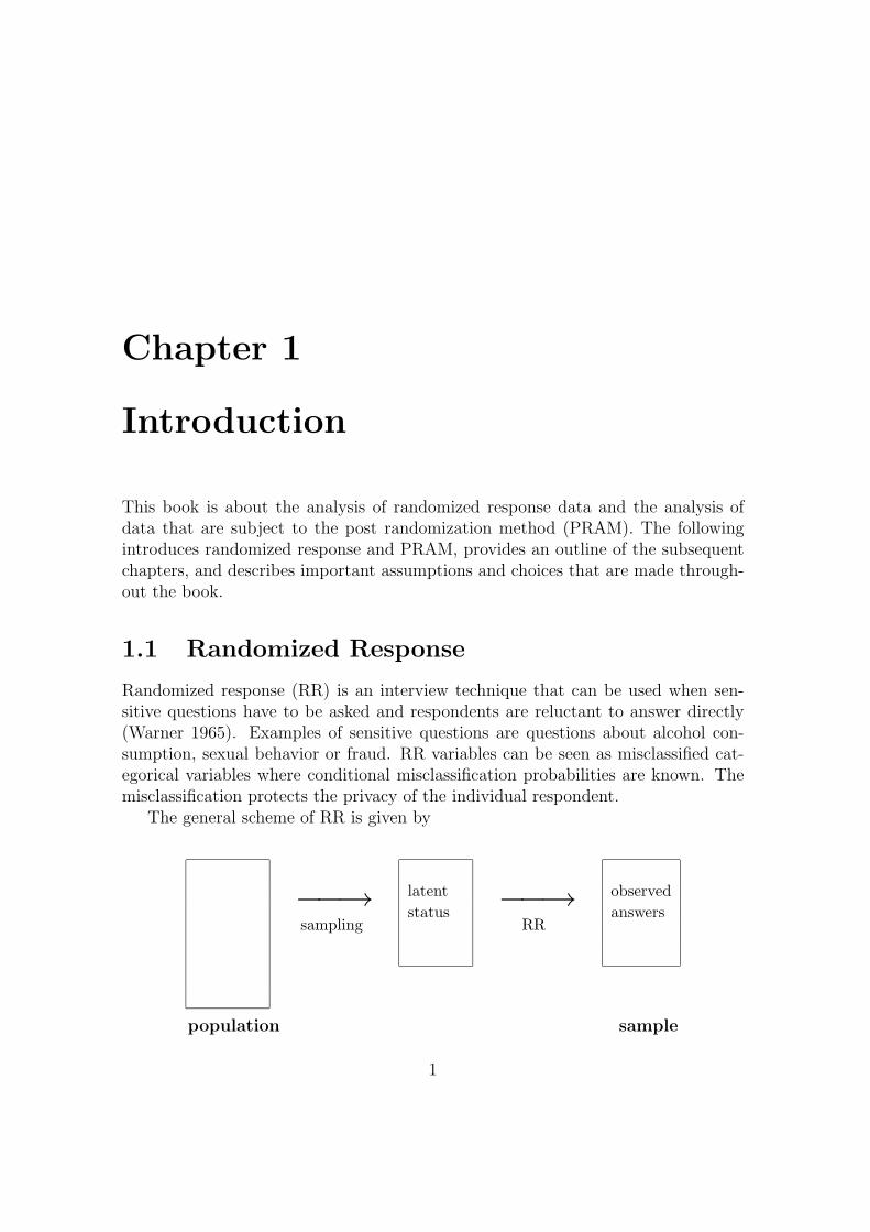
Randomized response (RR) is an interview technique that can be used when sen-sitive questions have to be asked and respondents are reluctant to answer directly(Warner 1965). Examples of sensitive questions are questions about alcohol con-sumption, sexual behavior or fraud. RR variables can be seen as misclassified cat-egorical variables where conditional misclassification probabilities are known. Themisclassification protects the privacy of the individual respondent.
The general scheme of RR is given by
−−→sampling
latentstatus −−→
RR
observedanswers
population sample
1
2 Chapter 1. Introduction
Assume that a researcher wants to assess a sensitive item and that he uses a ques-tion to which the answer is either yes or no. After the sample is drawn from thepopulation, the RR design is applied to the selected respondents. The latent statusof the respondents with respect to the sensitive item are unknown. Observed dataconsist of observed answers after RR is applied.
A possible choice of a RR design is the forced response design (Boruch 1971).In this design, the respondent throws two dice after the sensitive question is asked.The outcome of the dice is hidden from the interviewer. If the outcome is 2, 3 or 4,the respondent answers yes. If the outcome 5, 6, 7, 8, 9 or 10, he answers accordingto the truth. If the outcome 11 or 12, he answers no.
The RR design can be seen as a misclassification design. Assume that the sensi-tive question concerns fraud and that respondent Z indeed committed fraud. Whenthe question ”Did you commit fraud?” is asked in a direct response situation, thetruthful answer of Z is yes. Assume next that the forced response design is applied.When Z throws the dice and the outcome is 2, 3, 4, 5, 6, 7, 8, 9 or 10, he answersyes and he is correctly classified as a person that committed fraud. When the out-come is 11 or 12, the answer of Z is no and Z is misclassified as a person that didnot commit fraud. The misclassification probability conditional on the fact that Zcommitted fraud can be computed using the distribution of the outcome of the diceand is given by
IP ( Z is misclassified| Z committed fraud) = 1/12. (1.1)
When Z did not commit fraud, the misclassification probability is given by
IP ( Z is misclassified| Z did not commit fraud) = 1/6.
Since the interviewer does not know the outcome of the dice, the interviewer doesnot know whether the observed answer corresponds with the latent status of Z. Inother words, an observed yes does not necessarily mean that Z committed fraud.Hence the privacy of Z is protected.
Probability (1.1) is rather small and one might wonder whether the respondent issatisfied with the privacy protection that is offered. However, Moriarty and Wiseman(1976) showed that respondents tend to overestimate (1.1) due to an inaccurate ideaof the distribution of the outcome of the two dice.
More formally, let X be the binary RR variable that models the latent status,X∗ the binary variable that models the observed answer, and yes ≡ 1 and no ≡ 2.Given the forced response design, the distribution of X∗ is the 2-component finite
1.1. Randomized Response 3
mixture given by
IP (X∗ = x∗) =2∑
k=1
IP (X∗ = x∗|X = k)IP (X = k), (1.2)
where x∗ ∈ 1, 2. The conditional probabilities pjk = IP (X∗ = j|X = k) forj, k ∈ 1, 2 are fixed by the forced response design and the known distribution ofthe sum of the two dice. Formulation (1.2) shows that RR variables can be seenas misclassified variables. The transition matrix of X that contains the conditionalmisclassification probabilities pjk for j, k ∈ 1, 2 is given by
P X =
(p11 p12
p21 p22
)=
(11/12 2/121/12 10/12
).
Similar expressions hold for more that two RR variables or RR variables with morethan two categories.
Other RR designs are possible. A second example is the design where the mis-classification is based on drawing playing cards from two stacks (Kuk 1990). Inthis design, the misclassification is based on chosen distributions of the colors in thestacks. By choosing different distributions different misclassification probabilitiescan be determined.
In recent years, RR techniques have been investigated and applied in the Nether-lands. Van der Heijden, Van Gils, Bouts, and Hox (2000) compare two RR designswith face-to-face direct questioning. Boeije and Lensvelt-Mulders (2002) investigatecompliance and non-compliance in RR surveys. Van Gils, Van der Heijden, Laudy,and Ross (2003) report about rule transgression with respect to social benefits. Thetransgression was investigated using the RR design by Boruch (1971). Elffers, Vander Heijden, and Hezemans (2003) use RR to study rule transgression for two Dutchinstrumental laws. RR has also been studied outside the Netherlands. The mono-graph on RR by Chaudhuri and Mukerjee (1988) gives an overview of existing theoryand techniques.
The basic idea of RR is that the perturbation induced by the misclassificationdesign (in the first example, using the dice) protects the privacy of the respondentand that insight into the misclassification design (in the first example, the knowndistribution of the dice) can be used to analyze the data. A researcher who wantsto apply RR should reflect on two issues. The first is about the choice of the RRdesign and efficiency. How much protection does the design offer? Will respondentsunderstand the design? How expensive is the application? And, closely connectedwith cost, how many respondents are necessary? The second issue is connected with
4 Chapter 1. Introduction
the first and is about the analysis of the RR data. It is obvious that one should takecare of the misclassification due to the use of RR. How should that be done?
1.2 Post Randomization Method
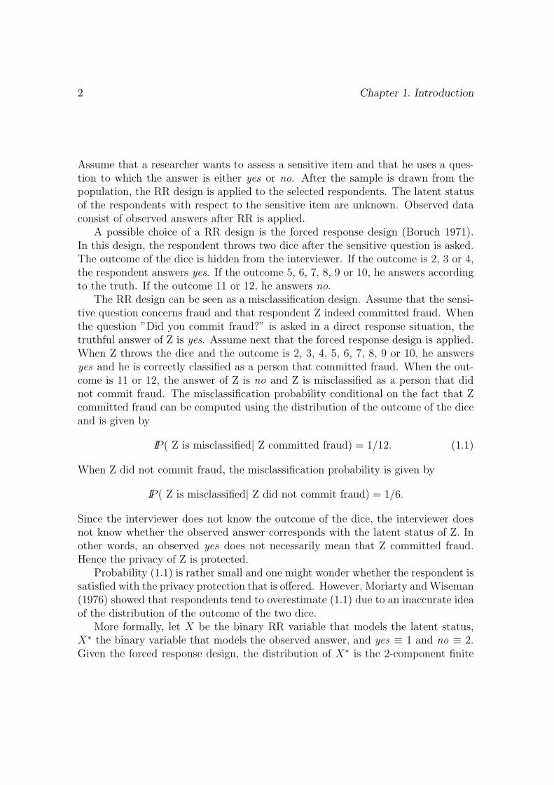
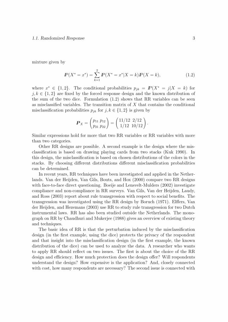
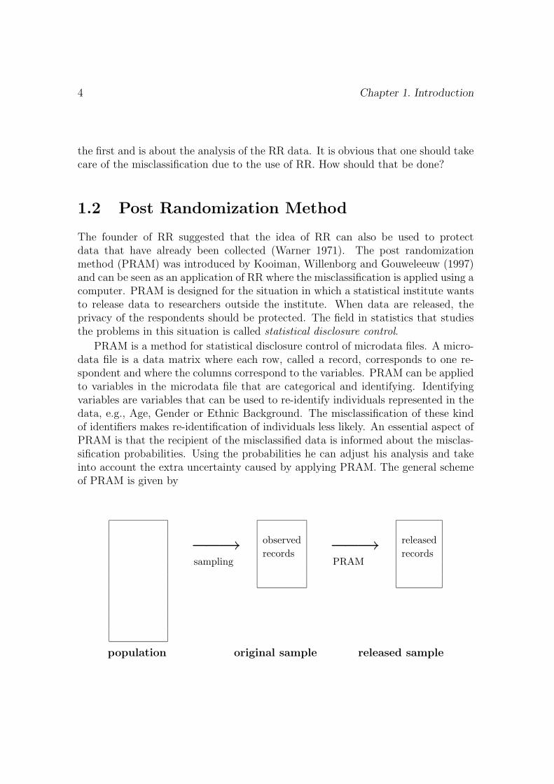
The founder of RR suggested that the idea of RR can also be used to protectdata that have already been collected (Warner 1971). The post randomizationmethod (PRAM) was introduced by Kooiman, Willenborg and Gouweleeuw (1997)and can be seen as an application of RR where the misclassification is applied using acomputer. PRAM is designed for the situation in which a statistical institute wantsto release data to researchers outside the institute. When data are released, theprivacy of the respondents should be protected. The field in statistics that studiesthe problems in this situation is called statistical disclosure control.
PRAM is a method for statistical disclosure control of microdata files. A micro-data file is a data matrix where each row, called a record, corresponds to one re-spondent and where the columns correspond to the variables. PRAM can be appliedto variables in the microdata file that are categorical and identifying. Identifyingvariables are variables that can be used to re-identify individuals represented in thedata, e.g., Age, Gender or Ethnic Background. The misclassification of these kindof identifiers makes re-identification of individuals less likely. An essential aspect ofPRAM is that the recipient of the misclassified data is informed about the misclas-sification probabilities. Using the probabilities he can adjust his analysis and takeinto account the extra uncertainty caused by applying PRAM. The general schemeof PRAM is given by
−−→sampling
observedrecords −−→
PRAM
releasedrecords
population original sample released sample
1.3. Outline of the Subsequent Chapters 5
The need for statistical disclosure control of microdata files is illustrated bythe following example. Assume that a general practitioner in the Netherlands is arespondent in a Dutch survey and that she was born in Bolivia. It is possible thatthis doctor is the only respondent in the sample that has the values (GP, Bolivia)of the combination of variables (Profession, Native Country). This means that herrecord might attract attention when the data are released without protection. Itmight be that a fellow doctor who happens to browse the sample file recognizesa former fellow student. Another more aggressive scenario is that someone triesto match records from the current survey to records from another survey in orderto look for discriminating information. The intentions of such an intruder may beobscure, yet a statistical institute that releases data should take the possibility ofsuch an attack into account. Hence the need for statistical disclosure control.
PRAM is not the only way to protect microdata against disclosure. Willen-borg and De Waal (2001) discuss alternative methods such as global recoding andlocal suppression. At Statistic Netherlands, PRAM was introduced by Kooiman,Willenborg and Gouweleeuw (1997). Subsequent research is presented by De Wolf,Gouweleeuw, Kooiman, and Willenborg (1997), Gouweleeuw, Kooiman, Willenborg,and De Wolf (1998), and Van den Hout (1999). PRAM is also one of the methodsdiscussed by Domingo-Ferrer and Torra (2001) who make a quantitative comparisonof disclosure control methods for microdata.
The two main issues concerning PRAM are comparable to the issues discussed inthe preceding section on RR: First, how to choose the misclassification probabilitiesin order to make the released microdata safe? Second, how should statistical analysisbe adjusted in order to take into account the misclassification? It is not difficult toprotect the privacy of respondents by perturbing data, the problem is to perturbthe data in such a way that the privacy is protected and the released data are usefulfor research.
1.3 Outline of the Subsequent Chapters
The basis of the subsequent chapters consists of five papers that are written forindividual publication. This structure has the advantage that the chapters are self-contained, a disadvantage is that there is some overlap in the discussion, especiallyin the introduction of the chapters. The outline is as follows.
Given the chosen conditional misclassification probabilities in the RR design or
6 Chapter 1. Introduction
the PRAM design, Chapter 2 discusses the estimation of proportions and the esti-mation of the odds ratio. The methods in this chapter can be used for questionslike: What is the percentage of persons that committed fraud? Or: Is there an as-sociation between committing fraud and gender? Moment estimates and maximumlikelihood estimates of the proportions are compared and it is proven that they arethe same in the interior of the parameter space. Special attention is paid to thepossibility of boundary solutions.
Chapter 3 can be seen as a generalization of the discussion in Chapter 2. Themethod in Chapter 3 can be used to investigate more dimensional association pat-terns. For example, a study is possible regarding the association between committingfraud, gender and population size of the place of residence. The chapter describesthe fitting of loglinear models to RR data and PRAM data. The misclassificationis described by a latent class model. Since a latent class model is a loglinear modelwith one or more categorical latent variables, it is possible to investigate relationsbetween misclassified variables. Methods to fit loglinear models for the latent ta-ble are discussed, including an EM algorithm. Again, attention is paid to problemswith boundary solutions. In an example, RR data are analyzed which were collectedusing the RR design by Kuk (1990).
Chapter 4 also discusses the fitting of loglinear models to RR data. There issome overlap with Chapter 3, but the situation is slightly different since a differentRR design is used and the use of RR is a factor in a 2 × 2 factorial design. Someof the respondents used the forced response design (Boruch 1971), others did not.The likelihood for this estimation problem is formulated and it is shown that alsoin this situation latent class software can be used to analyze the data. An exampleincluding a power analysis is discussed. This chapter shows the versatility of themodeling that is presented in Chapter 3.
Chapter 5 is about maximum likelihood estimation of the iid normal linear re-gression model when some of the independent variables are subject to RR or PRAM.An example of an application is the investigation of the relation between misclassi-fied independent variables Age, Gender, and Ethnic Background and non-perturbeddependent variable Income. The likelihood of the linear regression model with mis-classified independent variables is derived and a fast and straightforward EM al-gorithm is developed to obtain maximum likelihood estimates. The basis of thealgorithm consists of elementary weighted least squares steps.
The discussion in Chapter 6 concerns the application of PRAM. The chapterdiscusses two variants of the initial idea of PRAM regarding the information aboutthe misclassification that is given along with the released data. The first variantconcerns calibration probabilities and the second variant concerns misclassification
1.4. Assumptions and Choices 7
proportions. It is shown that the distinction between the univariate case and themultivariate case is important. In addition, the chapter discusses two measures fordisclosure risk when PRAM is applied.
1.4 Assumptions and Choices
The following describes the main assumptions and choices that are made throughoutthe book.
• The emphasis of the book is on analysis of misclassified data. How should weadjust standard statistical models in order to take into account the misclassifi-cation induced by either RR or PRAM? Chapter 6, which explicitly discussesPRAM, is an exception, since one of its topics is the relation between thechoice of the misclassification probabilities and the protection that is offered.
• Throughout the book the assumption is that respondents follow the RR design.This is a rather strong assumption. It is easy to imagine scenarios whererespondents do not follow the design, either because they do not understandit or because they do not trust the protection offered. At the end of Chapter3 this topic is briefly discussed.
• This book contains some real RR data examples. It is assumed that theresearch methods underlying the RR data are proper. Issues as sampling,questionnaires, interviewing, and data editing are not discussed.
• Since this book concerns applied statistics an effort is taken to make the dis-cussion accessible. Especially Chapters 2 and 3 go at some length to introduceconcepts, methods and solutions. Chapters 3 and 4 contain computer pro-grams that can be used to analyze the misclassified data. Another way inwhich the discussion is made more accessible is the linking of RR and PRAMto some well-known issues in social statistics such as the analysis of incompletedata and latent class analysis.

8
Chapter 2
Proportions and the Odds Ratio
2.1 Introduction
When scores on categorical variables are observed, there is a possibility of misclassi-fication. By a categorial variable we mean a stochastic variable which range consistsof a limited number of discrete values called the categories. Misclassification oc-curs when the observed category is i while the true category is j, i = j. Thispaper discusses analysis of categorical data subject to misclassification with knownmisclassification probabilities.
There are four fields in statistics where the misclassification probabilities areknown. The first is randomized response (RR). RR is an interview technique whichcan be used when sensitive questions have to be asked. Warner (1965) introducedthis technique and we use a simple form of the method as an introductory example.Let the sensitive question be ‘Have you ever used illegal drugs?’ The interviewerasks the respondent to roll a dice and to keep the outcome hidden. If the outcomeis 1,2,3 or 4 the respondent is asked to answer question Q, if the outcome is 5 or 6he is asked to answer Qc, where
Q = ‘Have you ever used illegal drugs?’
Qc = ‘Have you never used illegal drugs?’
The interviewer does not know which question is answered and observes only yesor no. The respondent answers Q with probability p = 2/3 and answers Qc withprobability 1 − p. Let π be the unknown probability of observing a yes-response to
1Published as Van den Hout and Van der Heijden (2002). Randomized response, statisticaldisclosure control and misclassification: a review, International Statistical Review 70, 269-288.
9
10 Chapter 2. Proportions and the Odds Ratio
Q. The probability of a yes-response is λ = pπ+(1−p)(1−π). So with the observedproportion as an estimate λ of λ, we can estimate π by
π =λ − (1 − p)
2p − 1. (2.1)
The main idea behind RR is that perturbation by the misclassification design(in this case the dice) protects the privacy of the respondent and that insight in themisclassification design (in this case the knowledge of the value of p) can be used toanalyze the observed data.
It is possible to create RR settings in which questions are asked to get informationon a variable with K > 2 categories (Chaudhuri and Mukerjee 1988, Chapter 3).We restrict ourselves in this paper to those RR designs of the form
λ = Pπ, (2.2)
where λ = (λ1, ..., λK)t is a vector denoting the probabilities of the observed re-sponses with categories 1, ..., K, π = (π1, ..., πK)t is the vector of the probabilitiesof the true responses and P is the K × K transition matrix of conditional misclas-sification probabilities pij, with
pij = IP (category i is observed| true category is j).
Note that this means that the columns of P add up to 1. In the Warner modelabove we have λ = (λ1, 1 − λ1)
t,
P =
(p 1 − p
1 − p p
),
and π = (π1, 1 − π1)t . Further background and more complex randomized response
schemes can be found in Fox and Tracy (1986) and Chaudhuri and Mukerjee (1988).The second field where the misclassification probabilities are known is the post
randomization method (PRAM), see Kooiman, Willenborg and Gouweleeuw (1997).The idea of PRAM is to misclassify the values of categorical variables after the datahave been collected in order to protect the privacy of the respondents by preventingdisclosure of their identities. PRAM can be seen as applying RR after the data havebeen collected. More information about PRAM and a comparison with RR is givenin Section 2.2.
The third field is statistics in medicine and epidemiology. In these disciplines,the probability to be correctly classified as a case given that one is a case is called
2.1. Introduction 11
the sensitivity, and the probability to be correctly classified as a non-case giventhat one is a non-case is called the specificity. In medicine, research concerningthe situation with known sensitivity and specificity is presented in Chen (1989)and Greenland (1980, 1988). In epidemiology, see Magder and Hughes (1997) andCopeland, Checkoway, McMichael, and Holbrook (1977).
The fourth field is the part of statistical astronomy that discusses rectificationand deconvolution problems. Lucy (1974), for instance, considers the estimation ofa frequency distribution where observations might be misclassified and where themisclassification probabilities are presumed known.
To present RR and PRAM as misclassification seems to be a logical approach,but a note must be made on this usage. Misclassification is a well known conceptwithin the analysis of categorical data and different methods to deal with this kindof perturbation have been proposed, see the review paper by Kuha and Skinner(1997), but the situation in which misclassification probabilities are known doesnot often occur. In most situations, these probabilities have to be estimated whichmakes analyses of misclassified data more complex.
The focus of this paper is on RR and PRAM. The discussion is about the analysisof the misclassified data, not about the choice of the misclassification probabilities.The central problem is: Given the data subject to misclassification and given thetransition matrix, how should we adjust standard analysis of frequency tables inorder to get valid results?
Special attention is given to the possibility of boundary solutions. By a boundarysolution we mean an estimated value of the parameter which lies on the boundary ofthe parameter space. For instance, in formula (2.1) the unbiased moment estimateof π is given. It is possible that this estimate is negative and makes no sense. Inthis case the moment estimate differs from the maximum likelihood estimate whichis zero and therefore lies on the boundary of the parameter space. This was alreadynoted by Singh (1976).
The possibility that the moment estimator yields estimates outside the parameterspace is an awkward property, since standard analyses as, e.g., univariate probabil-ities and the odds ratio, are in that case useless. However, negative estimates arelikely to occur when RR used. Typically, RR is applied when sensitive characteristicsare investigated and often sensitivity goes hand in hand with rareness. Therefore,some of the true frequencies in a sample may be low and when these frequenciesare unbiasedly estimated, random error can easily cause negative estimates. Theexample discussed in Section 2.7 illustrates this situation. Regarding PRAM thesame problem can occur, see Section 2.2.
This analysis of misclassified data has also been discussed by other authors, see
12 Chapter 2. Proportions and the Odds Ratio
the references above. Our present aim is to bring together the different fields ofmisclassification, compare the different methods, and propose methods to deal withboundary solutions. Noticeably lacking in some literature is a discussion of theproperties of proposed estimators such as unbiasedness and maximum likelihood.Where appropriate, we try to fill this gap.
Section 2.2 provides more information about PRAM. A comparison with RRis made. Section 2.3 discusses the moment estimator of the true frequency table,i.e., the not-observed frequencies of the correctly classified scores. Point estimatesand estimation of covariances are presented. In Section 2.4, we consider the maxi-mum likelihood estimation of the true frequency table. Again point estimation andvariances are discussed, this time using the EM algorithm. Section 2.5 relates themoment estimator to the maximum likelihood estimator. In Section 2.6, we con-sider the estimation of the odds ratio. In Section 2.7, an example is given with RRdata stemming from research into violating regulations of social benefit. Section 2.8evaluates the results and concludes.
2.2 Protecting Privacy Using PRAM
The post randomization method (PRAM) was introduced by Kooiman et al. (1997)as a method for statistical disclosure control of microdata files. A microdata file isa data matrix where each row, called a record, corresponds to one respondent andwhere the columns correspond to the variables. Statistical disclosure control (SDC)aims at safeguarding the identity of respondents. Because of the privacy protection,data producers, such as national statistical institutes, are able to pass on data to athird party.
PRAM can be applied to variables in the microdata file that are categoricaland identifying. Identifying variables are variables that can be used to re-identifyindividuals represented in the data. The perturbation of these identifiers makes re-identification of individuals less likely. The PRAM procedure yields a new microdatafile in which the scores on certain categorical variables in the original file may bemisclassified into different scores according to a given probability mechanism. Inthis way PRAM introduces uncertainty in the data: The user of the data cannotbe sure that the information in the file is original or perturbed due to PRAM. Inother words, the randomness of the procedure implies that matching a record in theperturbed file to a record of a known individual in the population could, with a highprobability, be a mismatch.
An important aspect of PRAM is that the recipient of the perturbed data is
2.2. Protecting Privacy Using PRAM 13
informed about the misclassification probabilities. Using these probabilities he canadjust his analysis and take into account the extra uncertainty caused by applyingPRAM.
As with RR, the misclassification scheme is given by means of a K×K transitionmatrix P of conditional probabilities pij, with
pij = IP (category i is released|true category is j).
Since national statistical institutes, which are the typical users of SDC methods,prefer model free approaches to their data, PRAM is presented in the form
IE[T ∗|T ] = PT , (2.3)
where T ∗ is the stochastic vector of perturbed frequencies and T is the vector of thetrue frequencies. So instead of using probabilities as in (2.2), frequencies are usedin (2.3) to avoid commitment to a specific parametric model.
PRAM is currently under study and is by far not the only way to protect mi-crodata against disclosure, see, e.g., Willenborg and De Waal (2001). Two commonmethods used by national statistical institutes are global recoding and local suppres-sion. Global recoding means that the number of categories is reduced by pooling,so that the new categories include more respondents than the original categories.This can be necessary when a category in the original file contains just a few re-spondents. For example, in a microdata file where the variable Profession has justone respondent with the value mayor, we can make a new category Working for theGovernment and include in this category not only the mayor, but also the peoplein the original file who have governmental jobs. The identity of the mayor is thenprotected not only by the number of people in the survey with governmental jobs,but also by the number of people in the population with governmental jobs.
Local suppression means protecting identities by making data missing. In theexample above, the identity of the mayor can be protected by making the valuemayor of the variable Profession missing.
When microdata are processed using recoding or suppression, there is always lossof information. This is inevitable: Losing information is intrinsic to SDC. Likewise,there will be loss of information when data are protected by applying PRAM.
PRAM is not meant to replace existing SDC techniques. Using the transitionmatrix with the misclassification probabilities to take into account the perturbationdue to PRAM, requires extra effort and becomes of course more complex whenthe research questions become more complex. This may not be acceptable to allresearchers. Nevertheless, existing SDC methods are also not without problems.
14 Chapter 2. Proportions and the Odds Ratio
Especially global recoding can destroy detail that is needed in the analysis. Forinstance, when a researcher has specific questions regarding teenagers becoming 18years old, it is possible that the data he wants to use is globally recoded before itis released. It is possible that the variable Age is recoded from year of birth to agecategories going from 0 to 5, 5 to 10, 10 to 15 , 15 to 20, etcetera. In that case, theresearcher has lost his object of research.
PRAM can be seen as a SDC method which can deal with specific requestsconcerning released data (such as in the foregoing paragraph) or with data whichare difficult to protect using current SDC methods (meaning the loss of informationis too large). PRAM can of course also be used in combination with other SDCmethods. Further information about PRAM can be found in Gouweleeuw, Kooiman,Willenborg and De Wolf (1998) and Van den Hout (1999).
The two basic research questions concering PRAM are (i) how to choose themisclassification probabilities in order to make the released microdata safe, and(ii) how should statistical analysis be adjusted in order to take into account themisclassification probabilities? As already stated in the introduction, this paperconcerns (ii). Our general objective is not only to present user-friendly methods inorder to make PRAM more user-friendly, but also to show that results in more thanone field in statistics can be used to deal with data perturbed by PRAM. Regarding(i), see Willenborg (2000) and Willenborg and De Waal (2001, Chapter 5).
Comparing (2.2) with (2.3), it can be seen that RR and PRAM are mathemat-ically equivalent. Therefore, PRAM is presented in this paper as a special formof RR. In fact, the idea of PRAM dates back from Warner (1971), the originatorof RR, who mentions the possibilities of the RR procedure to protect data afterthey have been collected. PRAM can be seen as applying RR after the data havebeen collected. Rosenberg (1979, 1980) elaborates the Warner idea and calls itadditive RR contamination (ARRC). PRAM turns out to be the same as ARRC.Rosenberg discusses multivariate analysis of data protected by ARRC, he discussesmultivariate categorical linear models and the chi-square test for contingency tables,in particular.
In the remainder of this section we make some comparisons between PRAM andRR. Since the methods serve different purposes, important differences may occurin practice. First, PRAM will be typically applied to those variables which maygive rise to the disclosure of the identity of a respondent, i.e., covariates as, e.g.,Gender, Age and Race. RR, on the other hand, will be typically applied to responsevariables, since the identifying covariates are obvious from the interview situation.Secondly, the usefulness of the observed response in the RR setting is dependent onthe cooperation of the respondent, whereas applying PRAM is completely mechanic.
2.3. Moment Estimator 15
Although RR may be of help in eliciting sensitive information, the method is not apanacea (Van der Heijden, Van Gils, Bouts, and Hox 2000). The third importantdifference concerns the choice of the transition matrix. When using RR the matrixis determined before the data are collected, but in the case of PRAM the matrixcan be determined conditionally on the original data. This means that the extentof randomness in applying PRAM can be controlled better than in the RR setting(Willenborg 2000).
PRAM is similar to RR regarding the possibility of boundary solutions, seeSection 2.1. PRAM is typically used when there are respondents in the sample withrare combinations of scores. Therefore, some of the true frequencies in a samplemay be low and when PRAM has been applied and these frequencies are unbiasedlyestimated, random error can easily cause negative estimates. So also regardingPRAM, methods to deal with boundary solutions are important.
2.3 Moment Estimator
This section generalizes (2.1) in order to obtain a moment estimator of the truecontingency table. A contingency table is a table with the sample frequencies ofcategorical variables. For example, the 2-dimensional contingency table of two bi-nary variables has four cells, each of which contains the frequency of a compoundedclass of the two variables. Section 2.3.1 presents the moment estimator for a m-dimensional table (m > 1). In Section 2.3.2 formulas to compute covariances arepresented.
2.3.1 Point Estimation
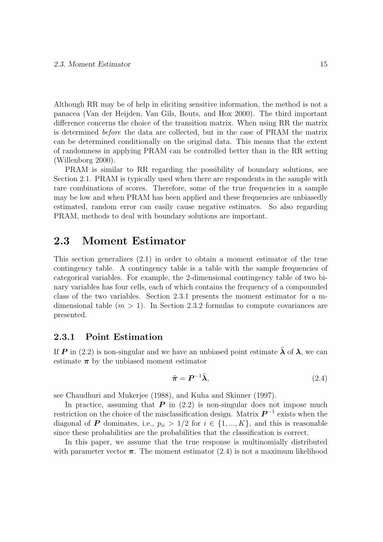
If P in (2.2) is non-singular and we have an unbiased point estimate λ of λ, we canestimate π by the unbiased moment estimator
π = P−1λ, (2.4)
see Chaudhuri and Mukerjee (1988), and Kuha and Skinner (1997).In practice, assuming that P in (2.2) is non-singular does not impose much
restriction on the choice of the misclassification design. Matrix P−1 exists when thediagonal of P dominates, i.e., pii > 1/2 for i ∈ 1, ..., K, and this is reasonablesince these probabilities are the probabilities that the classification is correct.
In this paper, we assume that the true response is multinomially distributedwith parameter vector π. The moment estimator (2.4) is not a maximum likelihood
16 Chapter 2. Proportions and the Odds Ratio
estimator since it is possible that for some i ∈ 1, ..., K, πi is outside the parameterspace (0,1).
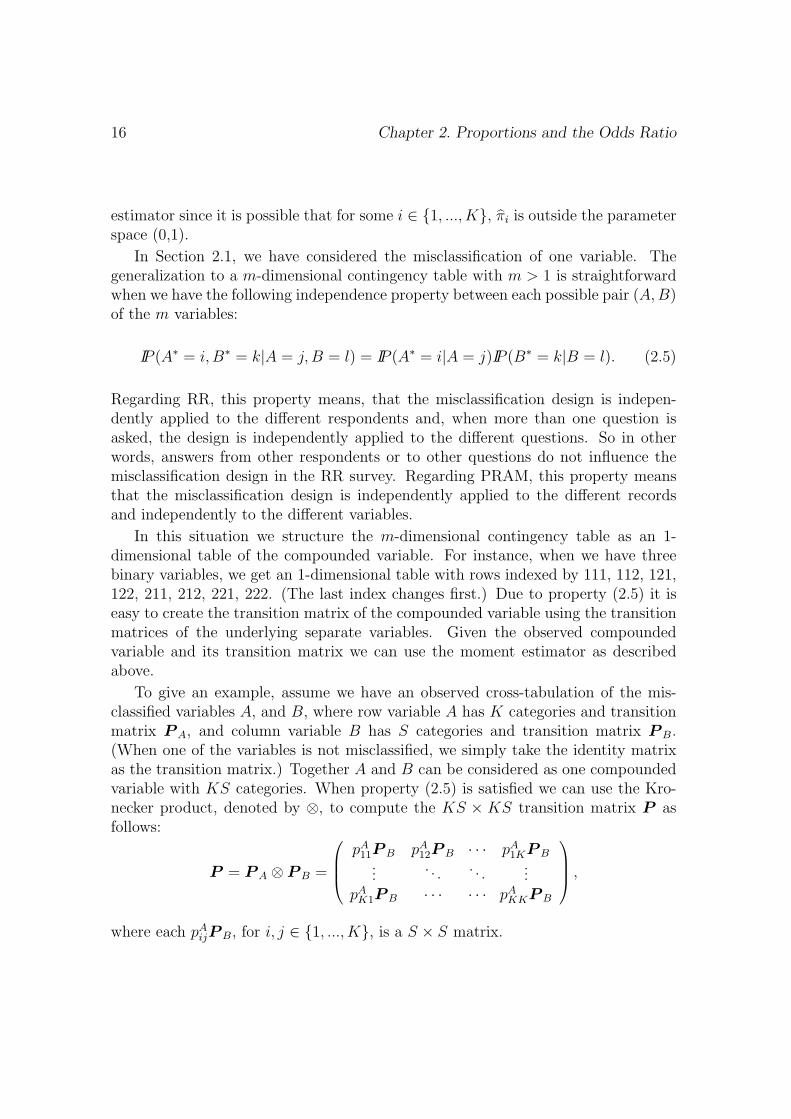
In Section 2.1, we have considered the misclassification of one variable. Thegeneralization to a m-dimensional contingency table with m > 1 is straightforwardwhen we have the following independence property between each possible pair (A,B)of the m variables:
IP (A∗ = i, B∗ = k|A = j, B = l) = IP (A∗ = i|A = j)IP (B∗ = k|B = l). (2.5)
Regarding RR, this property means, that the misclassification design is indepen-dently applied to the different respondents and, when more than one question isasked, the design is independently applied to the different questions. So in otherwords, answers from other respondents or to other questions do not influence themisclassification design in the RR survey. Regarding PRAM, this property meansthat the misclassification design is independently applied to the different recordsand independently to the different variables.
In this situation we structure the m-dimensional contingency table as an 1-dimensional table of the compounded variable. For instance, when we have threebinary variables, we get an 1-dimensional table with rows indexed by 111, 112, 121,122, 211, 212, 221, 222. (The last index changes first.) Due to property (2.5) it iseasy to create the transition matrix of the compounded variable using the transitionmatrices of the underlying separate variables. Given the observed compoundedvariable and its transition matrix we can use the moment estimator as describedabove.
To give an example, assume we have an observed cross-tabulation of the mis-classified variables A, and B, where row variable A has K categories and transitionmatrix P A, and column variable B has S categories and transition matrix P B.(When one of the variables is not misclassified, we simply take the identity matrixas the transition matrix.) Together A and B can be considered as one compoundedvariable with KS categories. When property (2.5) is satisfied we can use the Kro-necker product, denoted by ⊗, to compute the KS × KS transition matrix P asfollows:
P = P A ⊗ P B =
pA
11P B pA12P B · · · pA
1KP B...
. . . . . ....
pAK1P B · · · · · · pA
KKP B
,
where each pAijP B, for i, j ∈ 1, ..., K, is a S × S matrix.
2.4. Maximum Likelihood Estimator 17
2.3.2 Covariances
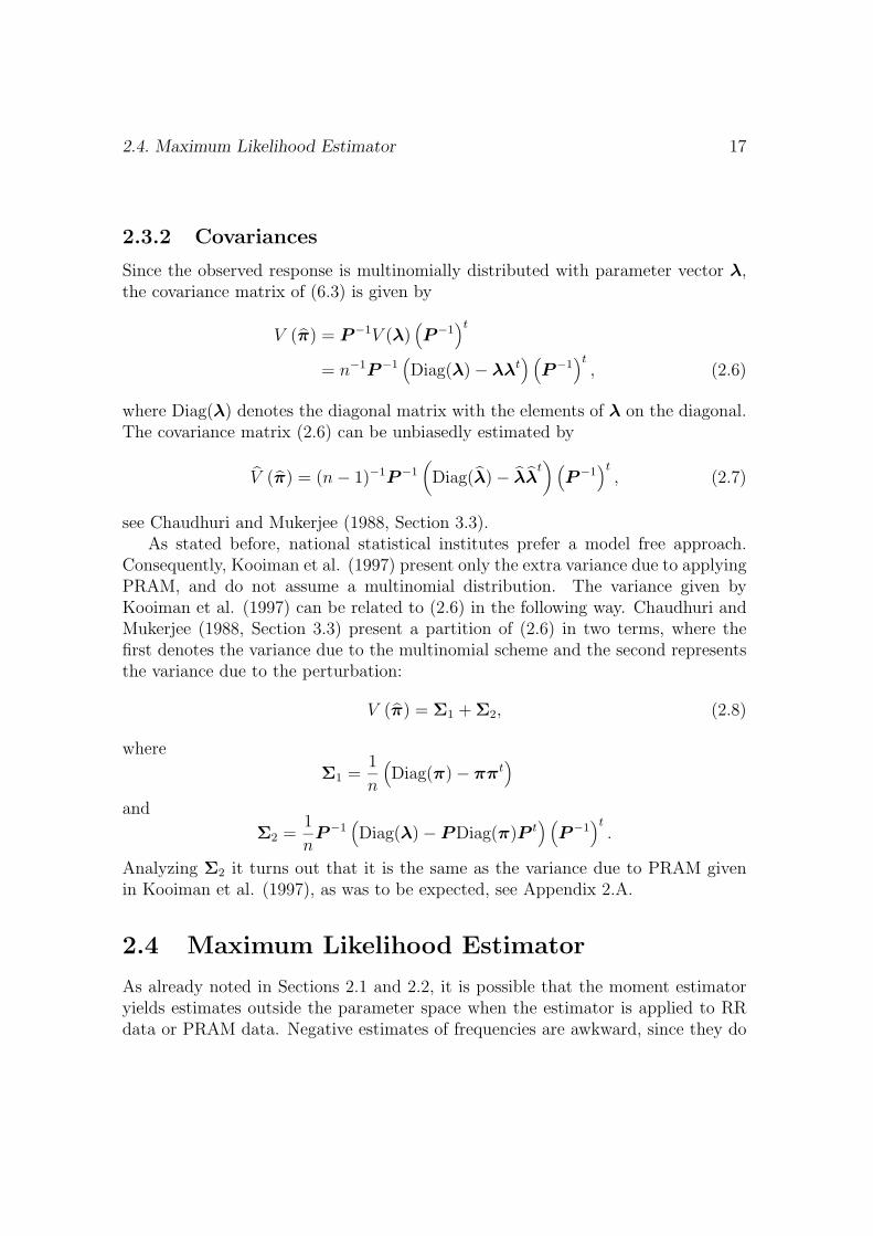
Since the observed response is multinomially distributed with parameter vector λ,the covariance matrix of (6.3) is given by
V (π) = P−1V (λ)(P−1
)t
= n−1P−1(Diag(λ) − λλt
) (P−1
)t, (2.6)
where Diag(λ) denotes the diagonal matrix with the elements of λ on the diagonal.The covariance matrix (2.6) can be unbiasedly estimated by
V (π) = (n − 1)−1P−1(Diag(λ) − λλ
t)(
P−1)t
, (2.7)
see Chaudhuri and Mukerjee (1988, Section 3.3).As stated before, national statistical institutes prefer a model free approach.
Consequently, Kooiman et al. (1997) present only the extra variance due to applyingPRAM, and do not assume a multinomial distribution. The variance given byKooiman et al. (1997) can be related to (2.6) in the following way. Chaudhuri andMukerjee (1988, Section 3.3) present a partition of (2.6) in two terms, where thefirst denotes the variance due to the multinomial scheme and the second representsthe variance due to the perturbation:
V (π) = Σ1 + Σ2, (2.8)
where
Σ1 =1
n
(Diag(π) − ππt
)and
Σ2 =1
nP−1
(Diag(λ) − PDiag(π)P t
) (P−1
)t.
Analyzing Σ2 it turns out that it is the same as the variance due to PRAM givenin Kooiman et al. (1997), as was to be expected, see Appendix 2.A.
2.4 Maximum Likelihood Estimator
As already noted in Sections 2.1 and 2.2, it is possible that the moment estimatoryields estimates outside the parameter space when the estimator is applied to RRdata or PRAM data. Negative estimates of frequencies are awkward, since they do
18 Chapter 2. Proportions and the Odds Ratio
not make sense. Furthermore, when there are more than two categories and thefrequency of one of them is estimated by a negative number, it is unclear how themoment estimate must be adjusted in order to obtain a solution in the parameterspace. This is a reason to look for a maximum likelihood estimate (MLE). Anotherreason to use MLEs is that in general, unbiasedness is not preserved when functionsof unbiased estimates are considered. Maximum likelihood properties on the otherhand, are in general preserved, see Mood, Graybill and Boes (1985).
This section discusses first the estimation of the MLE of the true contingencytable using the EM algorithm and, secondly, in 2.4.2, the covariances of this estimate.
2.4.1 Point Estimation
The expectation-maximization (EM) algorithm (Dempster, Laird and Rubin 1977)can be used as an iterative scheme to compute MLEs when data are incomplete, i.e.,when some observations are missing. The EM algorithm is in that case an alternativeto maximizing the likelihood function using methods as, e.g., the Newton-Raphsonmethod. Two appealing properties of the EM algorithm relative to Newton-Raphsonare its numerical stability and, given that the complete data problem is a standardone, the use of standard software for complete data analysis within the steps ofthe algorithm. These properties can make the algorithm quite user-friendly. Morebackground and recent developments can be found in McLachlan and Krishnan(1997).
We will now see how the EM algorithm can be used in a misclassification setting,see also Bourke and Moran (1988), Chen (1989), and Kuha and Skinner (1997). Forease of exposition we consider the 2×1 frequency table of a binary variable A. Asstated before, we assume multinomial sampling.
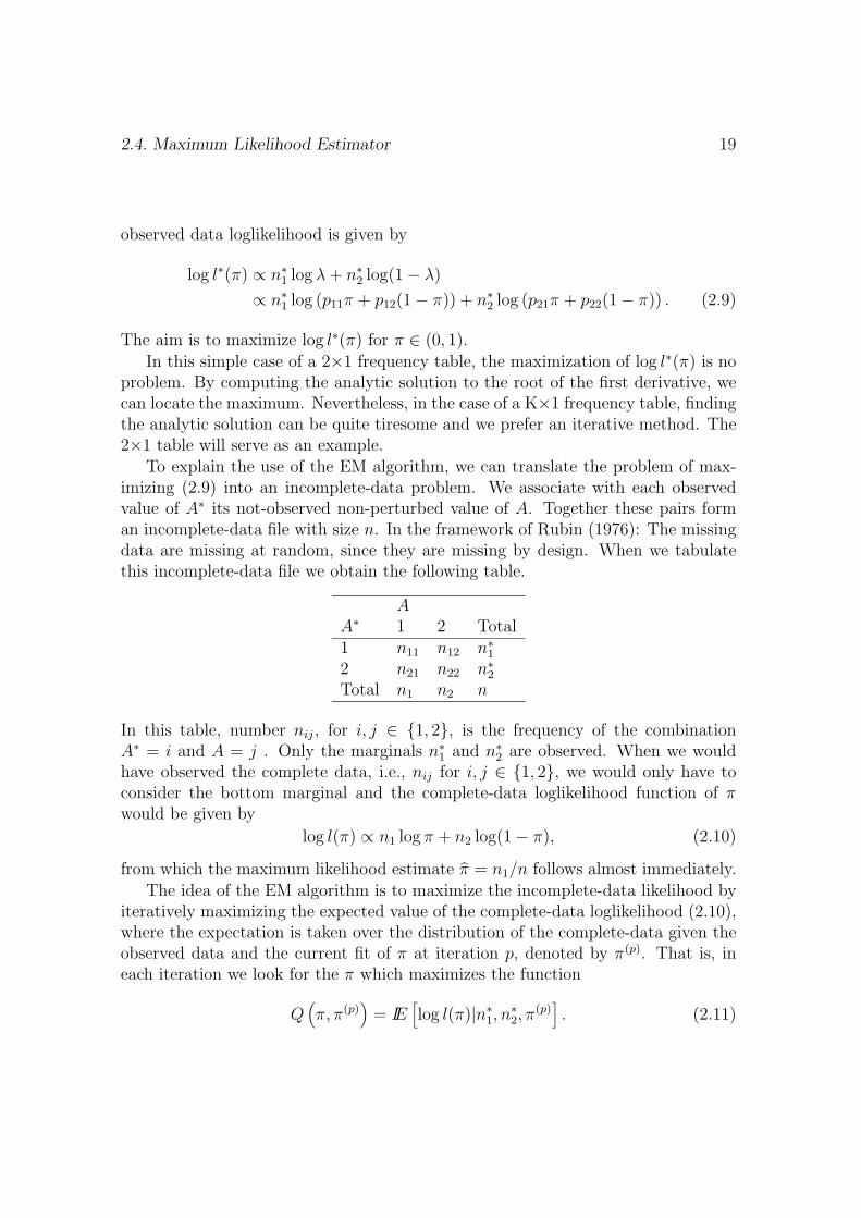
When the variable is subject to misclassification, say with given transition matrixP = (pij), we do not observe values of A, but instead we observe values of aperturbed A, say A∗. Let A∗ be tabulated as follows.
A∗
1 n∗1
2 n∗2
Total n
In this table, number n∗i , for i = 1, 2, is the observed number of values i of A∗
and n∗1 + n∗
2 = n is fixed. Let π = IP (A = 1) and λ = IP (A∗ = 1). When transitionprobabilities are given, we know λ = p11π + p12(1 − π). So ignoring constants, the
2.4. Maximum Likelihood Estimator 19
observed data loglikelihood is given by
log l∗(π) ∝ n∗1 log λ + n∗
2 log(1 − λ)
∝ n∗1 log (p11π + p12(1 − π)) + n∗
2 log (p21π + p22(1 − π)) . (2.9)
The aim is to maximize log l∗(π) for π ∈ (0, 1).In this simple case of a 2×1 frequency table, the maximization of log l∗(π) is no
problem. By computing the analytic solution to the root of the first derivative, wecan locate the maximum. Nevertheless, in the case of a K×1 frequency table, findingthe analytic solution can be quite tiresome and we prefer an iterative method. The2×1 table will serve as an example.
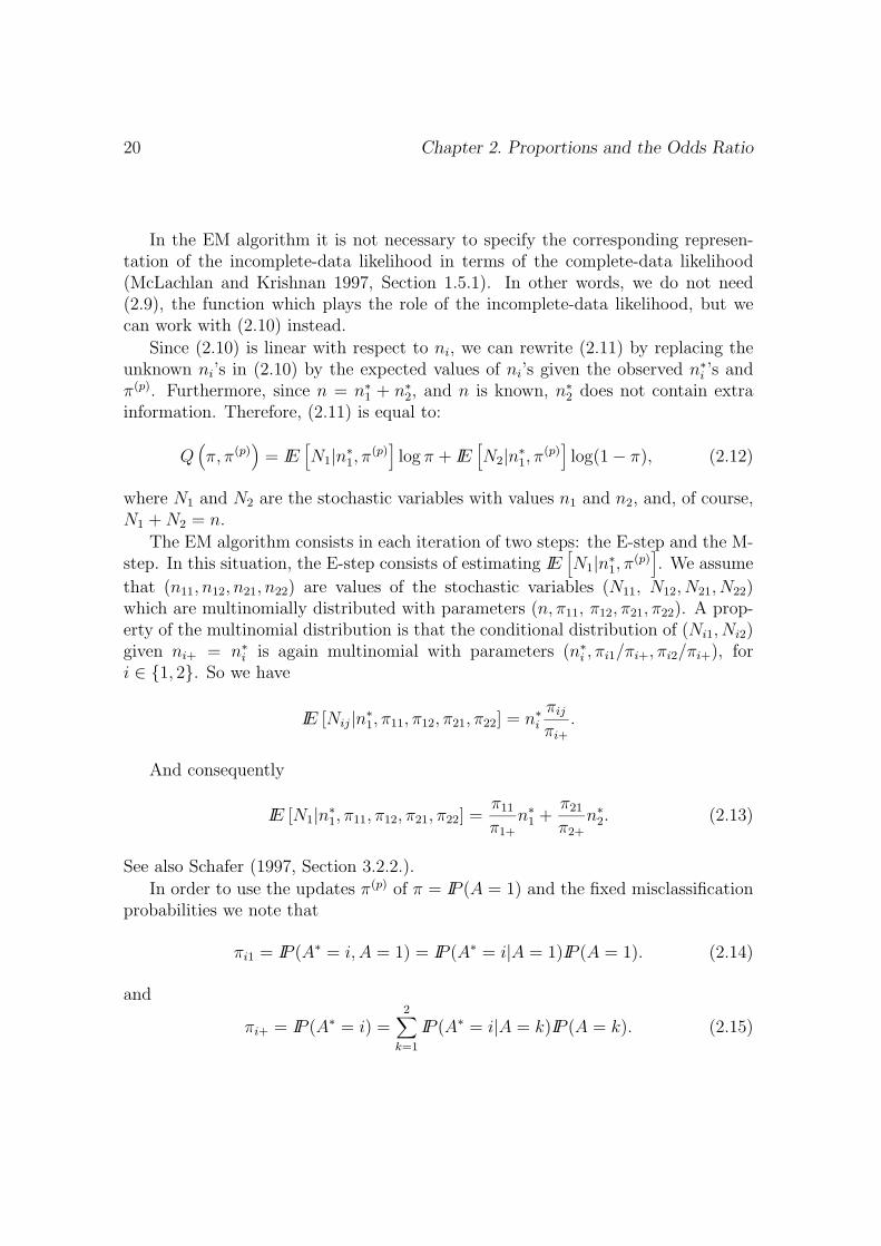
To explain the use of the EM algorithm, we can translate the problem of max-imizing (2.9) into an incomplete-data problem. We associate with each observedvalue of A∗ its not-observed non-perturbed value of A. Together these pairs forman incomplete-data file with size n. In the framework of Rubin (1976): The missingdata are missing at random, since they are missing by design. When we tabulatethis incomplete-data file we obtain the following table.
AA∗ 1 2 Total1 n11 n12 n∗
1
2 n21 n22 n∗2
Total n1 n2 n
In this table, number nij, for i, j ∈ 1, 2, is the frequency of the combinationA∗ = i and A = j . Only the marginals n∗
1 and n∗2 are observed. When we would
have observed the complete data, i.e., nij for i, j ∈ 1, 2, we would only have toconsider the bottom marginal and the complete-data loglikelihood function of πwould be given by
log l(π) ∝ n1 log π + n2 log(1 − π), (2.10)
from which the maximum likelihood estimate π = n1/n follows almost immediately.The idea of the EM algorithm is to maximize the incomplete-data likelihood by
iteratively maximizing the expected value of the complete-data loglikelihood (2.10),where the expectation is taken over the distribution of the complete-data given theobserved data and the current fit of π at iteration p, denoted by π(p). That is, ineach iteration we look for the π which maximizes the function
Q(π, π(p)
)= IE
[log l(π)|n∗
1, n∗2, π
(p)]. (2.11)
20 Chapter 2. Proportions and the Odds Ratio
In the EM algorithm it is not necessary to specify the corresponding represen-tation of the incomplete-data likelihood in terms of the complete-data likelihood(McLachlan and Krishnan 1997, Section 1.5.1). In other words, we do not need(2.9), the function which plays the role of the incomplete-data likelihood, but wecan work with (2.10) instead.
Since (2.10) is linear with respect to ni, we can rewrite (2.11) by replacing theunknown ni’s in (2.10) by the expected values of ni’s given the observed n∗
i ’s andπ(p). Furthermore, since n = n∗
1 + n∗2, and n is known, n∗
2 does not contain extrainformation. Therefore, (2.11) is equal to:
Q(π, π(p)
)= IE
[N1|n∗
1, π(p)]log π + IE
[N2|n∗
1, π(p)]log(1 − π), (2.12)
where N1 and N2 are the stochastic variables with values n1 and n2, and, of course,N1 + N2 = n.
The EM algorithm consists in each iteration of two steps: the E-step and the M-step. In this situation, the E-step consists of estimating IE
[N1|n∗
1, π(p)]. We assume
that (n11, n12, n21, n22) are values of the stochastic variables (N11, N12, N21, N22)which are multinomially distributed with parameters (n, π11, π12, π21, π22). A prop-erty of the multinomial distribution is that the conditional distribution of (Ni1, Ni2)given ni+ = n∗
i is again multinomial with parameters (n∗i , πi1/πi+, πi2/πi+), for
i ∈ 1, 2. So we have
IE [Nij|n∗1, π11, π12, π21, π22] = n∗
i
πij
πi+
.
And consequently
IE [N1|n∗1, π11, π12, π21, π22] =
π11
π1+
n∗1 +
π21
π2+
n∗2. (2.13)
See also Schafer (1997, Section 3.2.2.).
In order to use the updates π(p) of π = IP (A = 1) and the fixed misclassificationprobabilities we note that
πi1 = IP (A∗ = i, A = 1) = IP (A∗ = i|A = 1)IP (A = 1). (2.14)
and
πi+ = IP (A∗ = i) =2∑
k=1
IP (A∗ = i|A = k)IP (A = k). (2.15)
2.4. Maximum Likelihood Estimator 21
Next, we use (2.13), (2.14) and (2.15) to estimate IE[N1|n∗
1, π(p)]
by
n(p)1 =
2∑i=1
pi1π(p)
pi1π(p) + pi2 (1 − π(p))n∗
i ,
which ends the E-step.The M-step gives an update for π, which is the value of π that maximizes (2.12),
using the current estimate of IE[N1|n∗
1, π(p)], which also provides an estimate of
IE[N2|n∗
1, π(p)]
= n−IE[N1|n∗
1, π(p)]. Maximizing is easy due to the correspondence
between the standard form of (2.10) and the form of (2.12): π(p+1) = n(p)1 /n.
The EM algorithm is started with an initial value π(0). The following can bestated regarding the choice of the initial value and convergence of the algorithm.When there is a unique maximum in the interior of the parameter space, the EMalgorithm will find it, see the convergence theorems of the algorithm as discussedin McLachlan and Krishnan (1997, Section 3.4). Furthermore, as will be explainedin Section 2.5, in the RR/PRAM setting, the incomplete-data likelihood is from aregular exponential family and is therefore strictly concave, so finding the maximumshould not pose any difficulties when the starting point is chosen in the interior ofthe parameter space and the maximum is also achieved in the interior.
In general, let A have K categories and for i, j ∈ 1, 2, ..., K, let πj = IP (A = j),let nij denote the cell frequencies in the K × K table of A∗ and A, let nj denotethe frequencies in the K × 1 table of A, and let n∗
i denote the frequencies in theobserved K × 1 table of A∗. The observed data loglikelihood is given by
log l∗(π) =K∑
i=1
n∗i log λi + C (2.16)
where λi =∑K
k=1 pikπk and C is a constant.The EM algorithm in this situation and presented as such in Kuha and Skinner
(1997) is
Initial values: π(0)j =
n∗j
n
E-step: n(p)ij =
pijπ(p)j∑K
k=1 pikπ(p)k
n∗i
n(p)j =
K∑i=1
n(p)ij
22 Chapter 2. Proportions and the Odds Ratio
M-step: π(p+1)j =
n(p)j
n.
Note that π(p)j < 0 is not possible for j ∈ 1, 2, ..., K.
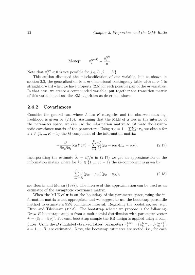
This section discussed the misclassification of one variable, but as shown insection 2.3, the generalization to a m-dimensional contingency table with m > 1 isstraightforward when we have property (2.5) for each possible pair of the m variables.In that case, we create a compounded variable, put together the transition matrixof this variable and use the EM algorithm as described above.
2.4.2 Covariances
Consider the general case where A has K categories and the observed data log-likelihood is given by (2.16). Assuming that the MLE of π lies in the interior ofthe parameter space, we can use the information matrix to estimate the asymp-totic covariance matrix of the parameters. Using πK = 1 −∑K−1
i=1 πi, we obtain fork, l ∈ 1, ..., K − 1 the kl-component of the information matrix:
− ∂
∂πk∂πl
log l∗(π) =K∑
i=1
n∗i
λ2i
(pil − piK)(pik − piK). (2.17)
Incorporating the estimate λi = n∗i /n in (2.17) we get an approximation of the
information matrix where for k, l ∈ 1, ..., K − 1 the kl-component is given by
K∑i=1
n
λi
(pik − piK)(pil − piK), (2.18)
see Bourke and Moran (1988). The inverse of this approximation can be used as anestimator of the asymptotic covariance matrix.
When the MLE of π is on the boundary of the parameter space, using the in-formation matrix is not appropriate and we suggest to use the bootstrap percentilemethod to estimate a 95% confidence interval. Regarding the bootstrap, see, e.g.,Efron and Tibshirani (1993). The bootstrap scheme we propose is the following.Draw B bootstrap samples from a multinomial distribution with parameter vectorπ = (π1, ..., πK)t. For each bootstrap sample the RR design is applied using a com-
puter. Using the B simulated observed tables, parameters πbootb =
(πboot
b1 , ..., πbootbK
)t,
b = 1, ..., B, are estimated. Next, the bootstrap estimates are sorted, i.e., for each
2.5. The MLE Compared to the Moment Estimate 23
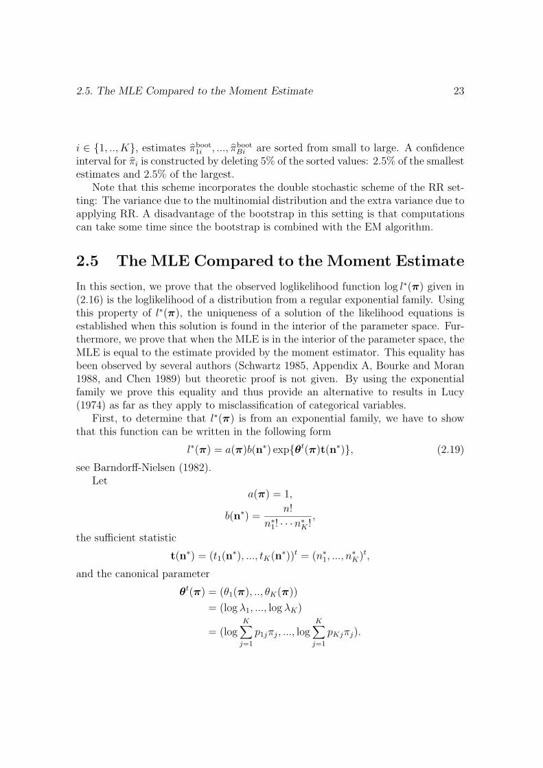
i ∈ 1, .., K, estimates πboot1i , ..., πboot
Bi are sorted from small to large. A confidenceinterval for πi is constructed by deleting 5% of the sorted values: 2.5% of the smallestestimates and 2.5% of the largest.
Note that this scheme incorporates the double stochastic scheme of the RR set-ting: The variance due to the multinomial distribution and the extra variance due toapplying RR. A disadvantage of the bootstrap in this setting is that computationscan take some time since the bootstrap is combined with the EM algorithm.
2.5 The MLE Compared to the Moment Estimate
In this section, we prove that the observed loglikelihood function log l∗(π) given in(2.16) is the loglikelihood of a distribution from a regular exponential family. Usingthis property of l∗(π), the uniqueness of a solution of the likelihood equations isestablished when this solution is found in the interior of the parameter space. Fur-thermore, we prove that when the MLE is in the interior of the parameter space, theMLE is equal to the estimate provided by the moment estimator. This equality hasbeen observed by several authors (Schwartz 1985, Appendix A, Bourke and Moran1988, and Chen 1989) but theoretic proof is not given. By using the exponentialfamily we prove this equality and thus provide an alternative to results in Lucy(1974) as far as they apply to misclassification of categorical variables.
First, to determine that l∗(π) is from an exponential family, we have to showthat this function can be written in the following form
l∗(π) = a(π)b(n∗) expθt(π)t(n∗), (2.19)
see Barndorff-Nielsen (1982).Let
a(π) = 1,
b(n∗) =n!
n∗1! · · ·n∗
K !,
the sufficient statistic
t(n∗) = (t1(n∗), ..., tK(n∗))t = (n∗
1, ..., n∗K)t,
and the canonical parameter
θt(π) = (θ1(π), .., θK(π))
= (log λ1, ..., log λK)
= (logK∑
j=1
p1jπj, ..., logK∑
j=1
pKjπj).
24 Chapter 2. Proportions and the Odds Ratio
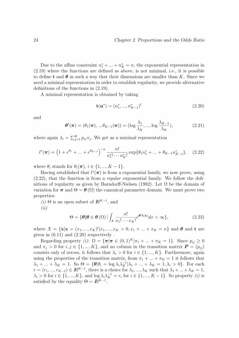
Due to the affine constraint n∗1 + ... + n∗
K = n, the exponential representation in(2.19) where the functions are defined as above, is not minimal, i.e., it is possibleto define t and θ in such a way that their dimensions are smaller than K. Since weneed a minimal representation in order to establish regularity, we provide alternativedefinitions of the functions in (2.19).
A minimal representation is obtained by taking
t(n∗) = (n∗1, ..., n
∗K−1)
t (2.20)
and
θt(π) = (θ1(π), .., θK−1(π)) = (logλ1
λK
, ..., logλK−1
λK
), (2.21)
where again λi =∑K
j=1 pijπj. We get as a minimal representation
l∗(π) =(1 + eθ1 + ... + eθK−1
)−n n!
n∗1! · · ·n∗
K !expθ1n
∗1 + ... + θK−1n
∗K−1, (2.22)
where θi stands for θi(π), i ∈ 1, ..., K − 1.Having established that l∗(π) is from a exponential family, we now prove, using
(2.22), that the function is from a regular exponential family. We follow the defi-nitions of regularity as given by Barndorff-Nielsen (1982). Let Ω be the domain ofvariation for π and Θ = θ (Ω) the canonical parameter domain. We must prove twoproperties:
(i) Θ is an open subset of IRK−1, and
(ii)
Θ = θ|θ ∈ θ (Ω) |∫
X
n!
x1! · · ·xK !eθtt(x)dx < ∞, (2.23)
where X = x|x = (x1, ..., xK)t|x1, ..., xK > 0, x1 + ... + xK = n and θ and t aregiven in (6.11) and (2.20) respectively .
Regarding property (i): Ω = π|π ∈ (0, 1)K |π1 + ... + πK = 1. Since pij ≥ 0and πj > 0 for i, j ∈ 1, ..., K, and no column in the transition matrix P = (pij)consists only of zeroes, it follows that λi > 0 for i ∈ 1, ..., K. Furthermore, againusing the properties of the transition matrix, from π1 + ... + πK = 1 it follows thatλ1 + ... + λK = 1. So Θ = θ|θi = log λiλ
−1K |λ1 + ... + λK = 1, λi > 0. For each
r = (r1, ..., rK−1) ∈ IRK−1, there is a choice for λ1, ..., λK such that λ1 + ...+λK = 1,λi > 0 for i ∈ 1, ..., K, and log λiλ
−1K = ri for i ∈ 1, ..., K − 1. So property (i) is
satisfied by the equality Θ = IRK−1.
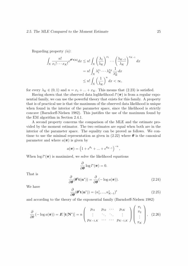
2.5. The MLE Compared to the Moment Estimate 25
Regarding property (ii):∫X
n!
x1! · · · xK !eθtt(x)dx ≤ n!
∫X
(λ1
λK
)x1
· · ·(
λK−1
λK
)xK−1
dx
= n!∫
Xλx1
1 · · ·λxKK
1
λnK
dx
≤ n!∫
X
(1
λK
)n
dx < ∞,
for every λK ∈ (0, 1) and n = x1 + ... + xK . This means that (2.23) is satisfied.Having shown that the observed data loglikelihood l∗(π) is from a regular expo-
nential family, we can use the powerful theory that exists for this family. A propertythat is of practical use is that the maximum of the observed data likelihood is uniquewhen found in the interior of the parameter space, since the likelihood is strictlyconcave (Barndorff-Nielsen 1982). This justifies the use of the maximum found bythe EM algorithm in Section 2.4.1.
A second property concerns the comparison of the MLE and the estimate pro-vided by the moment estimator. The two estimates are equal when both are in theinterior of the parameter space. The equality can be proved as follows. We con-tinue to use the minimal representation as given in (2.22) where θ is the canonicalparameter and where a(π) is given by
a(π) =(1 + eθ1 + ... + eθK−1
)−n,
When log l∗(π) is maximized, we solve the likelihood equations
∂
∂θlog l∗(π) = 0.
That is∂
∂θ(θtt(n∗)) =
∂
∂θ(− log a(π)). (2.24)
We have∂
∂θ(θtt(n∗)) = (n∗
1, ..., n∗K−1)
t (2.25)
and according to the theory of the exponential family (Barndorff-Nielsen 1982)
∂
∂θ(− log a(π)) = IE [t(N∗)] = n
p11 p12 · · · p1K...
. . . . . ....
pK−1,K · · · · · · pK−1,K
π1
π2...
πK
, (2.26)
26 Chapter 2. Proportions and the Odds Ratio
where N∗ is the random variable which has value n∗. Combining (2.25) and (2.26)in (2.24) shows that the likelihood equations (2.24) are equal to the equations (2.2)on which the moment estimator is based. So in the interior of the parameter space,the MLE is equal to the ME.
Of course, the above properties of l∗(π) can be derived without references to ex-ponential families. Lucy (1974) discusses the estimation of a frequency distributionwhere observations are subject to measurement error and the error distribution ispresumed known. The difference with our setting is that the observed variable isa continuous one. However, the observations are categorized in intervals and cor-rection of the observations is on the basis of these intervals, so measurement errorcan be easily translated to misclassification of categorical variables. Lucy (1974)advocates an EM algorithm comparable with the EM algorithm given above. Fur-thermore, it is proven that in the interior of the parameter space the MLE is equalto the moment estimate and the maximum of the likelihood is unique. In Appendix2.B we have translated Lucy’s proof regarding the equivalence between the MLEand the moment estimate to our setting.
2.6 Odds Ratio
This section discusses the estimation of the odds ratio when data are perturbedby PRAM or RR. The odds ratio θ is a measure of association for contingencytables. We will not go into the rationale of using the odds ratio, information aboutthis measure can be found in most textbooks on categorical data analysis, see, e.g.,Agresti (2002).
Section 2.6.1 discusses point estimation both in the situation without and withmisclassification. Two estimates of the odds ratio given by different authors are thesame, but are not always the MLE. Section 2.6.2 discusses the variance. Again, itis important whether the estimates of the original frequencies are in the interior ofthe parameter space or not.
2.6.1 Point Estimation
We start with the situation without misclassification. Let πij = IP (A = i, B = j)for i, j ∈ 1, 2 denote the probability that the scores for A and B fall in the cell inrow i and column j, respectively. The odds ratio is defined as
θ =π11π22
π12π21
.
2.6. Odds Ratio 27
With nij the observed frequency in the cell with probability πij. The sample oddsratio equals
θ =n11n22
n12n21
. (2.27)
For multinomial sampling, this is the MLE of the odds ratio (Agresti 1996). Thevalue 1 means independence of A and B. When any nij = 0, the sample odds ratioequals 0 or ∞. The sample odds ratio is not defined if both entries in a row orcolumn are zero.
It is possible to use sample proportions to compute the sample odds ratio. WithpA|B(i|j) = nij/(n1j + n2j) we get
θ =pA|B(1|1)
1 − pA|B(1|1)
(pA|B(1|2)
1 − pA|B(1|2)
)−1
. (2.28)
Next, we consider the situation with misclassification. Two estimates of the oddsratio are proposed in the literature. Let only variable A be subject to misclassifi-cation, and the 2×2 transition matrix be given by P = (pij). First, Magder andHughes (1997) suggest to adjust formula (2.28) as
θ1 =pA∗|B(1|1) − p12
p11 − pA∗|B(1|1)
(pA∗|B(1|2) − p12
p11 − pA∗|B(1|2)
)−1
, (2.29)
where pA∗|B(i|j) = n∗ij/(n
∗1j + n∗
2j) with n∗ij the observed cell frequencies. This
formula can be used only if all the numerators and denominators in the formula arepositive. If one of these is negative, the estimate is 0 or ∞. According to Magderand Hughes (1997), (2.29) is the MLE of θ. Assuming that θ1 is not equal to zeroor infinity, it will always be further from 1 than the odds ratio θ which is computedin the standard way using the observed table. Incorporating the information ofthe transition matrix in the estimation process compensates for the bias towards 1(Magder and Hughes 1997).
Secondly, Greenland (1988) suggests to estimate the probabilities of the truefrequencies using the moment estimator, yielding estimated frequencies nij = nπij,and then estimate the odds ratio using its standard form:
θ2 =n11n22
n12n21
. (2.30)
This procedure can also be used when A and B are both misclassified.In order to compare (2.29) and (2.30), we distinguish two situations concerning
the misclassification of only A. First, the situation where estimated frequencies
28 Chapter 2. Proportions and the Odds Ratio
are in the interior of the parameter space, or, in other words, where the momentestimate of the frequencies is equal to the MLE. In this case, (2.29) and (2.30) areidentical, which can be easily proved by writing out. Furthermore, (2.30), and thus(2.29), is the MLE due to the invariance property of maximum likelihood estimation(Mood et al. 1985).
Secondly, if the moment estimator yields probabilities outside the parameterspace, we should compute (2.30) using the MLE, and consequently (2.29) and (2.30)differ. In fact, (2.29) is not properly defined, since it might be a negative valuecorresponding to the negative cell frequencies estimated by the moment estimator.Therefore, as noted in Magder and Hughes (1997), the estimate of the odds ratioshould be adjusted to be either 0 or ∞.
The advantage of formula (2.29) is that we can use the observed table. A disad-vantage is that (2.29) is not naturally extended to the situation where two variablesare misclassified.
2.6.2 Variance
We now turn to the variance estimator of the odds ratio. First we describe thesituation without misclassification. Since outcomes nij = 0 have positive probability,
the expected value and variance of θ do not exist. It has been shown that
θ =(n11 + 0.5)(n22 + 0.5)
(n12 + 0.5)(n21 + 0.5)
has the same asymptotic normal distribution around θ as θ (Agresti 2002). Notethat θ has a variance. The close relation between θ and θ is the reason we willdiscuss asymptotic standard error (ASE) of log θ, although it is not mathematicallysound to do so.
There are at least two methods available to estimate the ASE of log θ. The firstmethod is using the delta method. The estimated ASE is then given by
ASE(log θ) =(
1
n11
+1
n12
+1
n21
+1
n22
)1/2
,
see Agresti (2002, Sections 3.1.5 and 14.1).The second method to estimate the ASE in the situation without misclassification
is to use the bootstrap. For instance, we can use the bootstrap percentile method toestimate a 95% confidence interval. When we assume the multinomial distribution,we take the vector of observed cell proportions as MLE of the cell probabilities.
2.7. Example 29
With this MLE we simulate a large number of multinomial tables and each timecompute the odds ratio. Then we estimate a 95% confidence interval in the sameway as described in Section 2.4.2.
Next, we consider the situation with misclassification. Along the line of the twomethods described above, we discuss two methods to estimate the variance of theestimate of the odds ratio. First, when the moment estimator is used, the delta-method can be applied to determine the variance of the log odds ratio. Greenland(1988) shows how this can be done when the transition matrix is estimated withknown variances. Our situation is easier, since the transition matrix is given. We usethe multivariate delta method (Bishop, Fienberg and Holland 1975, Section 14.6.3).The random vector is π = (π11, π12, π21, π22)
t with 4 × 4 asymptotic covariance-variance matrix V (π), see Section 2.3. We take the function f to be
f(π) = log(
π11π22
π12π21
),
which has a derivative at π ∈ (0, 1)4. The delta method provides the asymptoticvariance Vf for f(π):
Vf = (Df)tV (π)Df ,
where Df is the gradient vector of f at π and V (π) is given by (2.6).The problem with this method is that it makes use of the moment estimator
which only makes sense when this estimator yields a solution in the interior ofthe parameter space. A second way to estimate the variance is using the bootstrapmethod as explained in Section 2.4.2. in combination with the EM algorithm. Giventhat B is the number of bootstraps, the bootstrap will yield θ boot
1 , .., θ bootB and the
bootstrap percentile method can be used to estimate a 95% confidence interval.
2.7 Example
This section illustrates the foregoing by estimating tables of true frequencies on thebasis of data collected using RR. Also, in Section 2.7.2, an estimate of the oddsratio will be discussed. The example makes clear that boundary solutions can occurwhen RR is applied and that we need to apply methods such as the EM algorithmand the bootstrap.
2.7.1 Frequencies
The RR data we want to analyze stem from a research into violating regulations ofsocial benefit (Van Gils, Van der Heijden, and Rosebeek 2001). Sensitive items were
30 Chapter 2. Proportions and the Odds Ratio
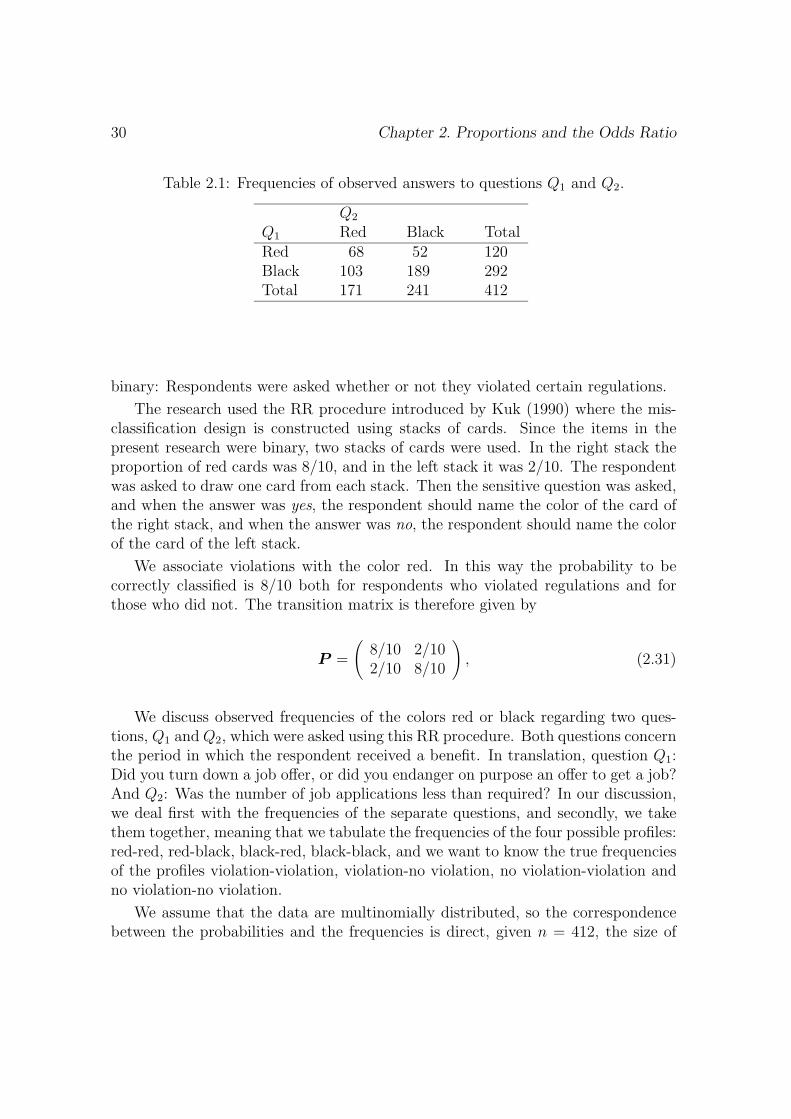
Table 2.1: Frequencies of observed answers to questions Q1 and Q2.
Q2
Q1 Red Black TotalRed 68 52 120Black 103 189 292Total 171 241 412
binary: Respondents were asked whether or not they violated certain regulations.
The research used the RR procedure introduced by Kuk (1990) where the mis-classification design is constructed using stacks of cards. Since the items in thepresent research were binary, two stacks of cards were used. In the right stack theproportion of red cards was 8/10, and in the left stack it was 2/10. The respondentwas asked to draw one card from each stack. Then the sensitive question was asked,and when the answer was yes, the respondent should name the color of the card ofthe right stack, and when the answer was no, the respondent should name the colorof the card of the left stack.
We associate violations with the color red. In this way the probability to becorrectly classified is 8/10 both for respondents who violated regulations and forthose who did not. The transition matrix is therefore given by
P =
(8/10 2/102/10 8/10
), (2.31)
We discuss observed frequencies of the colors red or black regarding two ques-tions, Q1 and Q2, which were asked using this RR procedure. Both questions concernthe period in which the respondent received a benefit. In translation, question Q1:Did you turn down a job offer, or did you endanger on purpose an offer to get a job?And Q2: Was the number of job applications less than required? In our discussion,we deal first with the frequencies of the separate questions, and secondly, we takethem together, meaning that we tabulate the frequencies of the four possible profiles:red-red, red-black, black-red, black-black, and we want to know the true frequenciesof the profiles violation-violation, violation-no violation, no violation-violation andno violation-no violation.
We assume that the data are multinomially distributed, so the correspondencebetween the probabilities and the frequencies is direct, given n = 412, the size of
2.7. Example 31
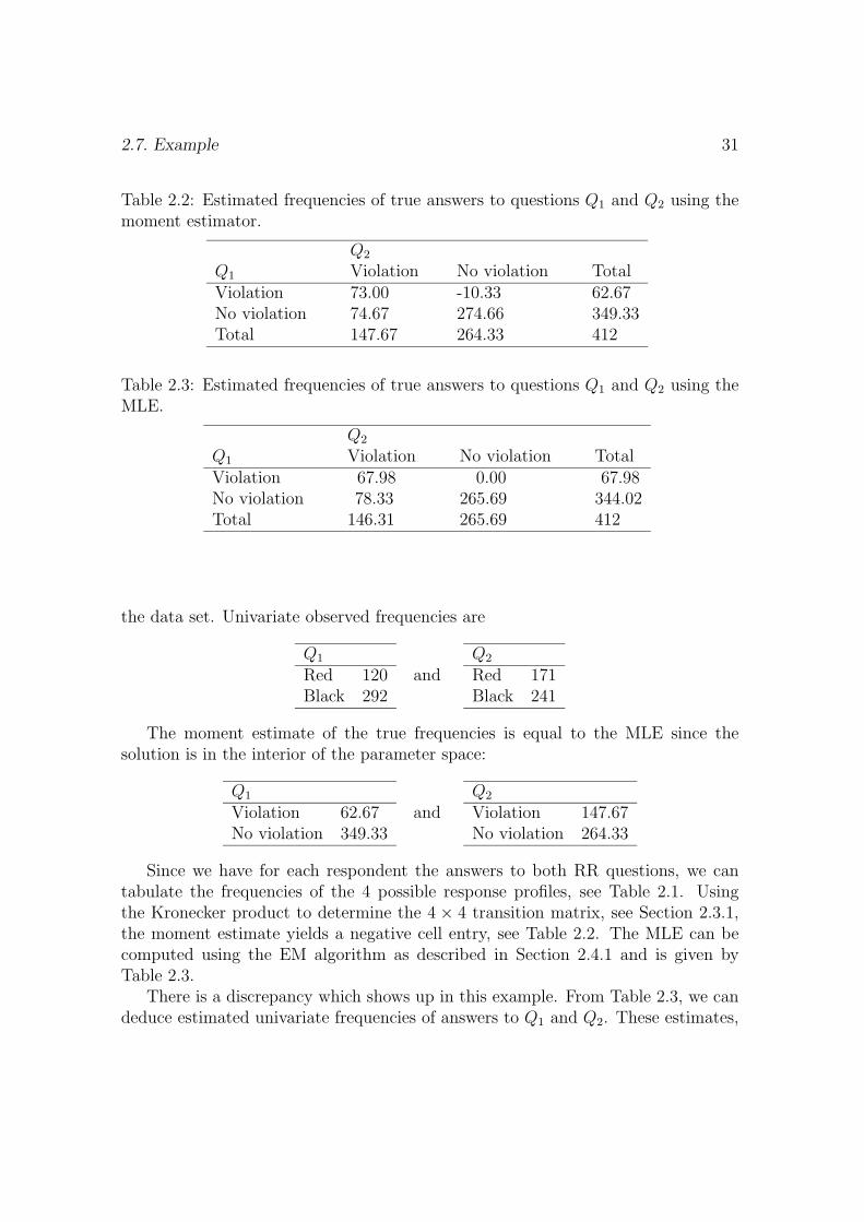
Table 2.2: Estimated frequencies of true answers to questions Q1 and Q2 using themoment estimator.
Q2
Q1 Violation No violation TotalViolation 73.00 -10.33 62.67No violation 74.67 274.66 349.33Total 147.67 264.33 412
Table 2.3: Estimated frequencies of true answers to questions Q1 and Q2 using theMLE.
Q2
Q1 Violation No violation TotalViolation 67.98 0.00 67.98No violation 78.33 265.69 344.02Total 146.31 265.69 412
the data set. Univariate observed frequencies are
Q1
Red 120Black 292
andQ2
Red 171Black 241
The moment estimate of the true frequencies is equal to the MLE since thesolution is in the interior of the parameter space:
Q1
Violation 62.67No violation 349.33
andQ2
Violation 147.67No violation 264.33
Since we have for each respondent the answers to both RR questions, we cantabulate the frequencies of the 4 possible response profiles, see Table 2.1. Usingthe Kronecker product to determine the 4 × 4 transition matrix, see Section 2.3.1,the moment estimate yields a negative cell entry, see Table 2.2. The MLE can becomputed using the EM algorithm as described in Section 2.4.1 and is given byTable 2.3.
There is a discrepancy which shows up in this example. From Table 2.3, we candeduce estimated univariate frequencies of answers to Q1 and Q2. These estimates,
32 Chapter 2. Proportions and the Odds Ratio
which are based on the MLE of the true multivariate frequencies are different fromthe univariate moment estimates which are also MLEs. Differences however aresmall.
Next, we turn to the estimation of variance. First, the univariate case, where weonly discuss question Q1. The estimated probability of violation is π = 62.67/412 =0.152. The estimated standard error of π can be computed using (2.7) and is esti-mated to be 0.037. Secondly, we compute the variance of the four estimated proba-bilities concerning profiles of violation. From Table 2.3 we obtain π = (π1, ..., π4)
t =(0.17, 0.00, 0.19, 0.64)t. Since the MLE is on the boundary of the parameter space,estimating a 95% confidence interval is more useful than estimating standard errors.We use the bootstrap percentile method as explained in Section 2.4.2. and withB = 500 we obtain the four intervals [0.09, 0.23], [0.00, 0.08], [0.11, 0.28], and [0.53,0.72], for π = (π1, ..., π4)
t.
2.7.2 Odds Ratio
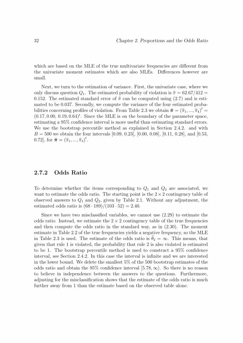
To determine whether the items corresponding to Q1 and Q2 are associated, wewant to estimate the odds ratio. The starting point is the 2×2 contingency table ofobserved answers to Q1 and Q2, given by Table 2.1. Without any adjustment, theestimated odds ratio is (68 · 189)/(103 · 52) = 2.40.
Since we have two misclassified variables, we cannot use (2.29) to estimate theodds ratio. Instead, we estimate the 2× 2 contingency table of the true frequenciesand then compute the odds ratio in the standard way, as in (2.30). The momentestimate in Table 2.2 of the true frequencies yields a negative frequency, so the MLEin Table 2.3 is used. The estimate of the odds ratio is θ2 = ∞. This means, thatgiven that rule 1 is violated, the probability that rule 2 is also violated is estimatedto be 1. The bootstrap percentile method is used to construct a 95% confidenceinterval, see Section 2.4.2. In this case the interval is infinite and we are interestedin the lower bound. We delete the smallest 5% of the 500 bootstrap estimates of theodds ratio and obtain the 95% confidence interval [5.78,∞〉. So there is no reasonto believe in independence between the answers to the questions. Furthermore,adjusting for the misclassification shows that the estimate of the odds ratio is muchfurther away from 1 than the estimate based on the observed table alone.
2.8. Conclusion 33
2.8 Conclusion
The aim of this paper is to review the different fields of misclassification where mis-classification probabilities are known, and to compare estimators of the true con-tingency table and the odds ratio. Special attention goes out to the possibility ofboundary solutions. The matrix based moment estimator is quite elegant, but thereare problems concerning solutions outside the parameter space. We have explainedand illustrated with the example that these problems are likely to occur when ran-domized response or PRAM is applied, since these procedures are often applied toskewed distributions. The maximum likelihood estimator is a good alternative tothe moment estimator but demands more work since the likelihood function is maxi-mized numerically using the EM algorithm. When boundary solutions are obtained,we suggest the bootstrap method to compute confidence intervals.
The proof of the equality of the moment estimate and the maximum likelihoodestimate, when these estimates are in the interior of the parameter space, is interest-ing because it establishes theoretically what was conjectured by others on the basisof numerical output.
Regarding PRAM, the results are useful in the sense that they show that fre-quency analysis with the released data is possible and that there is ongoing researchin the field of RR and misclassification which deals with the problems that are en-countered. This is important concerning the acceptance of PRAM as a SDC method.
Regarding RR, the example illustrates that a boundary solution may be encoun-tered in practice. This possibility was also noted by others but is, as far as we know,not investigated in the multivariate situation with attention to the estimation ofstandard errors.
Appendix 2.A
As stated in Section 2.3.2, V (π) can be partitioned as
V (π) = Σ1 + Σ2, (2.32)
where
Σ1 =1
n
(Diag(π) − ππt
)and
Σ2 =1
nP−1
(Diag(λ) − PDiag(π)P t
) (P−1
)t. (2.33)
34 Chapter 2. Proportions and the Odds Ratio
To understand (2.32):
Σ1 + Σ2 =1
n
(Diag(π) − ππt + P−1Diag(λ)
(P−1
)t − Diag(π))
=1
n
(P−1Diag(λ)
(P−1
)t − ππt)
=1
nP−1
(Diag(λ) − PππtP t
) (P−1
)t
=1
nP−1
(Diag(λ) − λλt
) (P−1
)t
= V (π)
The variance due to PRAM as given in Kooiman et al. (1997) equals
V(T |T
)= P−1V (T ∗|T )
(P−1
)t
= P−1
K∑j=1
T (j)V j
(P−1
)t(2.34)
where for j ∈ 1, ..., K, T (j) is the true frequency of category j, and V j is theK ×K covariance matrix of two observed categories h and i given the true categoryj:
V j(h, i) =
pij(1 − pij) if h = i
−phjpij if h = i, for h, i ∈ 1, ..., K, (2.35)
(Kooiman et al. 1997).In order to compare (2.33) with (6.5), we go from probabilities to frequencies in
the RR data. This is no problem since we assume the RR data to be distributedmultinomially. So we have V
(T |T
)= n2V (π|π) where, analogous to the PRAM
data, T denotes the vector with the true frequencies.In order to prove that n2Σ2 is the same as (6.5), it is sufficient to prove that
K∑j=1
T (j)V j = Diag(T ∗) − PDiag(T )P t
=
∑j p1jT (j) 0 · · · 0
0∑
j p2jT (j)...
.... . . 0
0 · · · 0∑
j pKjT (j)
− PDiag(T ) (P )t ,
which follows by writing out.
Appendix 35
Appendix 2.B
As stated in Section 2.5, Lucy (1974) proves that in the interior of the parameterspace the MLE of the true frequencies is equal to the moment estimate. In thefollowing we have translated this proof to our setting and put in some explanatorysteps.
The function we want to maximize for π ∈ (0, 1)K under the constraint∑K
j=1 πj =1, is
log l∗(π) =K∑
i=1
n∗i log λi + C (2.36)
where n∗i is given, λi =
∑Kk=1 pikπk, for i ∈ 1, ..., K, and C is a constant.
We start by maximizing for π ∈ IRK and we look for the stationary points ofthe function
G(π, µ) =K∑
i=1
n∗i log λi − µ
K∑j=1
πj − 1
(2.37)
where µ is the Lagrange multiplier. Setting the derivatives of G with respect to πj
and µ equal to zero, we obtain
∂
∂πj
G(π, µ) =K∑
i=1
n∗i
pij
λi
+ µ = 0 (2.38)
and∂
∂µG(π, µ) =
K∑j=1
πj − 1 = 0. (2.39)
Multiplying (2.38) with πj and summing over j yields
K∑j=1
K∑i=1
n∗i
pijπj
λi
= −µK∑
j=1
πj.
Using (2.39) we find that µ = −∑Ki=1 n∗
i = −n. With this result it follows that theequality in (2.38) holds if πj for j ∈ 1, ..., K is such that
K∑i=1
λipij
λi
= 1,
where λi = n∗i /n for i ∈ 1, ..., K. Since the transition matrix P has the property
that∑K
i=1 pij = 1, the equality in (2.38) holds if πj, for j ∈ 1, ..., K, is such that
λi = λi for i ∈ 1, ..., K.

36 Chapter 2. Proportions and the Odds Ratio
In other words, a stationary point of (2.37) is found for such π that
λ = Pπ.
To conclude, when (2.36) has one maximum under the constraint∑K
j=1 πj = 1,
this maximum is attained at the moment estimator π = P−1λ.When we include the constraint π ∈ (0, 1)K and we maximize under this extra
constraint, the MLE is not equal to the moment estimate when the moment estimateis outside the parameter space (0, 1)K .
Chapter 3
Loglinear Analysis
3.1 Introduction
Randomized response (RR) is an interview technique that can be used when sensitivequestions have to be asked (Warner 1965; Chaudhuri and Mukerjee 1988). RR datacan be seen as misclassified data where conditional misclassification probabilitiesare known. The main purpose of this paper is to show how research questionsconcerning association patterns in multivariate RR data can be assessed using latentclass models (Haberman 1979; Hagenaars 1993). Describing the RR design by alatent class model (LCM) is an advantage in practice since software to assess LCMsis widely available, e.g, the program EM (Vermunt 1997).
In addition, this paper considers problems with respect to boundary solutions inthe loglinear models that we want to fit. As far as we know, these problems are notdiscussed in the literature. As will be shown by examples, boundary solutions canoccur when analyzing RR data and in that situation one should take care regardingthe formulation of the EM algorithm. We review the discussion in Kuha and Skinner(1997) and Chen (1989), in which the EM algorithm is used for loglinear analysis ofmisclassified data.
As an example, RR data concerning violations of regulations for social benefitare analyzed. Sensitive items were binary: Respondents were asked whether theyhad violated certain regulations (Van Gils, Van der Heijden and Rosebeek 2001).
The outline of the paper is as follows. Section 3.2 introduces the RR designand misclassification designs that are closely related. Section 3.3 discusses the chi-
1Published as Van den Hout and Van der Heijden (2004). The analysis of multivariate misclas-sified data with special attention to randomized response data, Sociological Methods and Research32, 310-336.
37
38 Chapter 3. Loglinear Analysis
square test of independence and introduces some of the techniques that are used inthe following sections. In Section 3.4, the RR design is described by a latent classmodel and consequently loglinear models for RR data are presented and an exampleis given. Section 3.5 presents techniques for fitting the loglinear models to RR data.The likelihood is given, and the EM algorithm in the literature is discussed. InSection 3.6, attention is paid to boundary solutions and bias in RR data. Section3.7 concludes.
3.2 The Randomized Response Design
The research by Van Gils et al. (2001) used the RR design introduced by Kuk(1990). In this design, there are two stacks of cards each containing black and redcards. In the right stack the proportion of red cards is 8/10, and in the left stack2/10. The respondent is asked to draw one card from each stack and to keep thecolor of the cards hidden from the interviewer. Next, the sensitive question is asked.Instead of answering the question directly with yes or no, the respondent namesthe color of the card he took from the related stack, i.e., when the answer is yes,the respondent names the color of the card he or she took from the right stack, andwhen the answer is no, he or she names the color of the card from the left stack.
RR data can be described as misclassified data. We associate violations withthe color red. In this way, the probability to be correctly classified is 8/10 both forrespondents who violated regulations and for those who did not. The RR matrixthat contains the conditional misclassification probabilities
pij = IP (category i is observed| true category is j) (3.1)
is therefore given by
P =
(p11 p12
p21 p22
)=
(8/10 2/102/10 8/10
). (3.2)
The main idea behind RR is that the perturbation induced by the misclassi-fication design (in this case, the red and black cards) protects the privacy of therespondent and that insight in the misclassification design (in this case, the knowl-edge of the proportions red/black) can be used to analyze the observed data.
It is possible to create RR designs in which questions are asked to get informationabout a variable with K > 2 categories, see, e.g., Chaudhuri and Mukerjee (1988,Chapter 3). The general form of the RR designs we discuss is
θ∗ = Pθ, (3.3)
3.2. The Randomized Response Design 39
where θ∗ = (θ∗1, ..., θ∗K)t is a vector denoting the probabilities of the observed answers
with categories 1, ..., K; θ = (θ1, ..., θK)t is the vector of the probabilities of the trueanswers; and P is the K × K transition matrix of conditional misclassificationprobabilities pij, as given in (3.1). Note that this means that the columns of P addup to 1. Further background and more complex randomized response designs canbe found in Chaudhuri and Mukerjee (1988) and Fox and Tracy (1986).
Since we are dealing with the general form of misclassification as given in (3.3),the methods discussed in this paper can also be used in categorical data analysiswhere misclassification occurs and the probabilities given by (3.1) are known. Anexample is known sensitivity and specificity in epidemiologic research, see, e.g.,Magder and Hughes (1997).
There is also a similarity between RR designs and the post randomization method(PRAM), introduced by Kooiman, Willenborg, and Gouweleeuw (1997) as a methodfor statistical disclosure control of data matrices. Statistical disclosure control aimsat safeguarding the identity of respondents. Because of the privacy protection,data producers, such as national statistical institutes, are able to pass on datato a third party. The PRAM procedure yields a new data matrix in which thevalues of certain categorical variables in the original matrix may be misclassified intodifferent values according to a given probability mechanism. In this way, PRAMintroduces uncertainty in the data: The user of the data cannot be sure whetherthe information in the matrix is original or perturbed due to PRAM. As with RR,the misclassification scheme is given by means of a K × K transition matrix P ofconditional probabilities pij, where
pij = IP (category i is released|true category is j).
The role of the transition matrix in the analysis of PRAM data is the same as therole of the transition matrix in the analysis of RR data. More about PRAM andthe similarity with RR can be found in Van den Hout and Van der Heijden (2002).
A third field that may benefit from results regarding misclassification with knownmisclassification probabilities is data mining. In this field, huge amounts of data arecollected from surfers on the web, and privacy concerns initiated research into waysto protect the privacy of surfers by intentional statistical perturbation (Evfimievski,Srikant, Agrawal, and Gehrke 2002).
Specific to the misclassification induced by RR is that it is nondifferential andindependent. Let A and B denote two categorical variables, where A has I categoriesand B has J categories. Let A∗ and B∗ be the misclassified versions of A and B.Misclassification of A is called nondifferential with respect to B if
IP (A∗ = k| A = i, B = j) = IP (A∗ = k| A = i), (3.4)
40 Chapter 3. Loglinear Analysis
where k, i ∈ 1, 2, ..., I and j ∈ 1, 2, ..., J, see Kuha and Skinner (1997). Thenotion of independence is used when there are more than two misclassified variables.The misclassification is independent if
IP (A∗ = k, B∗ = l| A = i, B = j) = IP (A∗ = k| A = i, B = j)
× IP (B∗ = l| A = i, B = j), (3.5)
where k, i ∈ 1, 2, ..., I and l, j ∈ 1, 2, ..., J.If P in (3.3) is non-singular and we have an unbiased estimate θ
∗of θ∗, we can
estimate θ by the unbiased moment estimator
θ = P−1θ∗, (3.6)
(Chaudhuri and Mukerjee 1988; Kuha and Skinner 1997). In practice, assumingthat P in (3.3) is non-singular does not impose much restriction on the choice of themisclassification design. Matrix P−1 exists when the diagonal of P dominates −−that is, pii > 1/2 for i ∈ 1, ..., K −− and this is reasonable since these probabilitiesare the probabilities that the classification is correct.
Due to the fact that the misclassification in a RR design is independent andnondifferential, the generalization to an m-dimensional contingency table with m >1 is straightforward. First, the m-dimensional contingency table is structured asan 1-dimensional table of a compounded variable. For instance, when we havethree binary variables, we obtain an one-dimensional table with rows indexed by111, 112, 121, 122, 211, 212, 221, 222 (the last index changes first). Second, dueto the properties (3.4) and (3.5), it is possible to create the transition matrix ofthe compounded variable using the transition matrices of the underlying variables.Given the observed compounded variable and its transition matrix, we can use themoment estimator as described above.
3.3 Chi-Square Test of Independence
This section discusses testing independence between two categorical variables whereone variable or both variables are subject to misclassification due to a RR designsuch as (3.3).
Consider the cross-tabulation of the variables A and B, which are defined inthe previous section. Let πij = IP (A = i, B = j) for each i ∈ 1, 2, .., I andj ∈ 1, 2, .., J. The data are assumed to be distributed multinomially. The nullhypothesis of independence is H0 : πij = πi+π+j, where the plus sign denotes sum-mation over the related index, e.g., πi+ = πi1 + ... + πiJ . In the standard situation
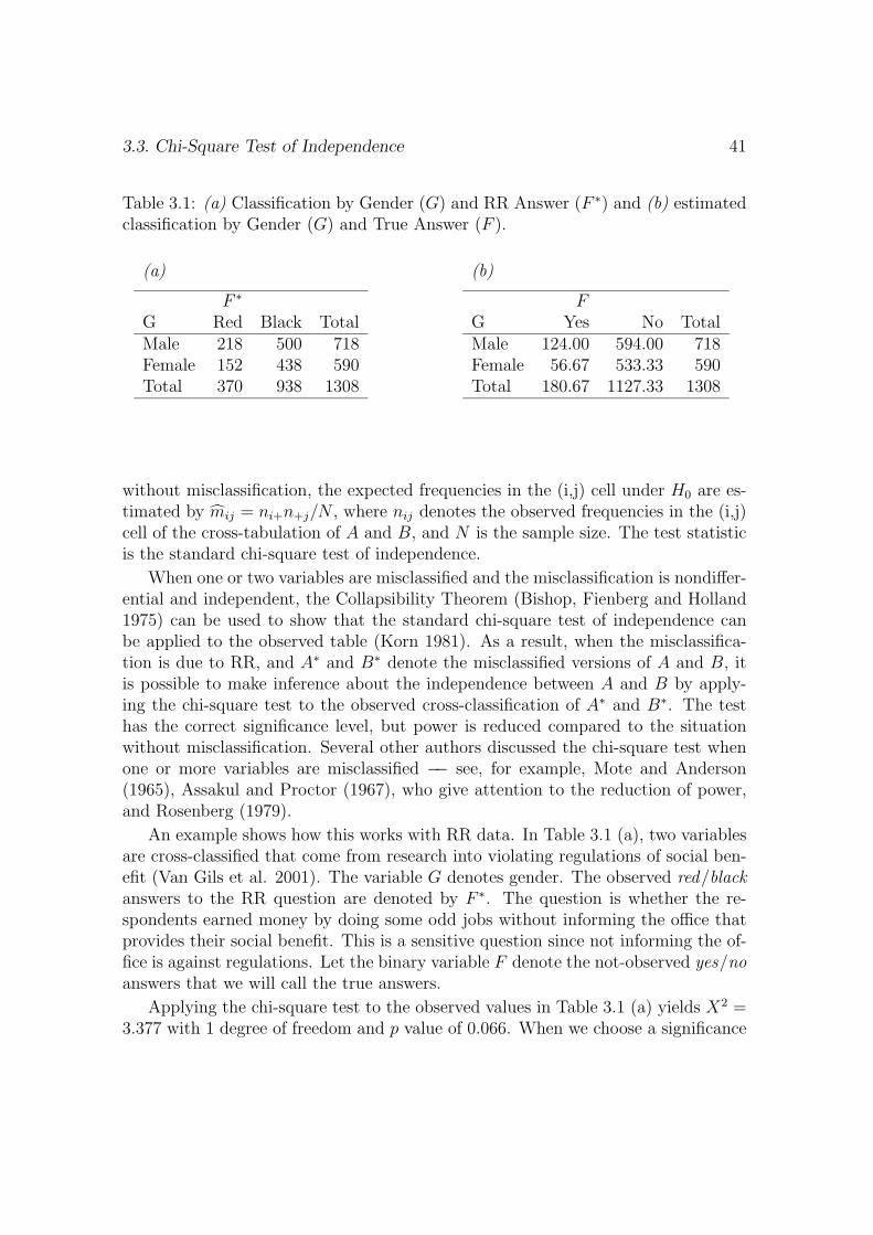
3.3. Chi-Square Test of Independence 41
Table 3.1: (a) Classification by Gender (G) and RR Answer (F ∗) and (b) estimatedclassification by Gender (G) and True Answer (F ).
(a)
F ∗
G Red Black TotalMale 218 500 718Female 152 438 590Total 370 938 1308
(b)
FG Yes No TotalMale 124.00 594.00 718Female 56.67 533.33 590Total 180.67 1127.33 1308
without misclassification, the expected frequencies in the (i,j) cell under H0 are es-timated by mij = ni+n+j/N , where nij denotes the observed frequencies in the (i,j)cell of the cross-tabulation of A and B, and N is the sample size. The test statisticis the standard chi-square test of independence.
When one or two variables are misclassified and the misclassification is nondiffer-ential and independent, the Collapsibility Theorem (Bishop, Fienberg and Holland1975) can be used to show that the standard chi-square test of independence canbe applied to the observed table (Korn 1981). As a result, when the misclassifica-tion is due to RR, and A∗ and B∗ denote the misclassified versions of A and B, itis possible to make inference about the independence between A and B by apply-ing the chi-square test to the observed cross-classification of A∗ and B∗. The testhas the correct significance level, but power is reduced compared to the situationwithout misclassification. Several other authors discussed the chi-square test whenone or more variables are misclassified −− see, for example, Mote and Anderson(1965), Assakul and Proctor (1967), who give attention to the reduction of power,and Rosenberg (1979).
An example shows how this works with RR data. In Table 3.1 (a), two variablesare cross-classified that come from research into violating regulations of social ben-efit (Van Gils et al. 2001). The variable G denotes gender. The observed red/blackanswers to the RR question are denoted by F ∗. The question is whether the re-spondents earned money by doing some odd jobs without informing the office thatprovides their social benefit. This is a sensitive question since not informing the of-fice is against regulations. Let the binary variable F denote the not-observed yes/noanswers that we will call the true answers.
Applying the chi-square test to the observed values in Table 3.1 (a) yields X2 =3.377 with 1 degree of freedom and p value of 0.066. When we choose a significance
42 Chapter 3. Loglinear Analysis
level of α = 0.05, the data do not give a reason to reject the null hypothesis.We now show that ignoring the results of Korn (1981) and taking the misclas-
sification into account leads to the same value of X2. Let n∗ = (n∗11, n
∗12, n
∗21, n
∗22)
t
denote the observed frequencies in Table 3.1 (a). To use the moment estimator (6.3),we first define the transition matrix P GF of the compounded variable. Since theRR design for F is applied with matrix (3.2) and gender (G) is not perturbed, weobtain
P GF =
8/10 2/10 0 02/10 8/10 0 0
0 0 8/10 2/100 0 2/10 8/10
. (3.7)
This matrix is used to estimate frequencies n = (n11, n12, n21, n22)t in the classifica-
tion by G and F byn = P−1
GF n∗,
see Table 3.1 (b). Next, we estimate the expected frequencies in this table, denotedby m= (m11, m12, m21, m22)
t, under the model of independence by mij = ni+n+j/N .Since we want to fit the model of independence, we compute the fitted frequenciesunder this model, denoted by m∗, by
m∗ = P GF m
and compare them with the observed n∗. Again we get X2 = 3.377.When measuring the association between G and F by estimating the odds ratio,
the misclassification should be taken into account explicitly. To show this, we willfirst ignore the misclassification and, second, give the adjusted estimate of the oddsratio.
Using only Table 3.1 (a) to compute an estimate of the odds ratio η in thestandard way, yields η∗ = (218×438)/(500×152) = 1.26. The large-sample standarderror of log η∗ is (1/218 + 1/500 + 1/152 + 1/438)1/2 = 0.12, see Agresti (2002), sothat η∗ has the 95% confidence interval [0.99; 1.61]. This interval includes 1 anddoes therefore not justify rejecting the null hypothesis of independence. However,this estimate of η is biased towards 1 (Magder and Hughes 1997) and is thereforenot trustworthy.
An adjusted estimate can be deduced from Table 3.1 (b): η = (124.00×533.33)/(594.00×56.67) = 1.96. The logarithm of this estimate has a large-sample standarderror of 0.40, so that η has 95% confidence interval [0.90; 4.29], see Greenland (1988)and Van den Hout and Van der Heijden (2002). As expected, the interval is largerthan the interval of η∗ since the extra variance due to the RR design is taken into
3.4. The Loglinear Model 43
account. We see that, in accordance with the chi-square test to the observed valuesin Table 3.1 (a), the adjusted estimation of the odds ratio does not justify rejectingH0.
3.4 The Loglinear Model
This section discusses loglinear analysis where one or more categorical variablesare observed using a RR design such as (3.3). This section can be seen as anextension to Section 3.3 since testing the loglinear model of independence for twovariables is equal to the chi-square test of independence. First, we use the loglinearparameterization of the LCM to show that the RR design can be described by aLCM. Second, we give an example of loglinear analysis where one of the variablesis an RR variable. The link between RR and LCMs is useful since it turns out thatwidely available latent class software can be used to fit loglinear models that containRR variables.
When one or more variables in the standard loglinear model concern observedvalues in a RR design, loglinear analysis using only the observed table may lead towrong inference about the parameters. Consider, for instance, the variables G andF ∗ that are cross-classified in Table 3.1 (a). The standard saturated model (GF ∗)to describe this table is given by
log mgf∗ = λ0 + λGg + λF ∗
f∗ + λGF ∗gf∗ ,
where mgf∗ denotes the expected frequency in the (g, f ∗) cell, and g, f ∗ ∈ 1, 2.The λ terms are restricted by
2∑g=1
λGg =
2∑f∗=1
λF ∗f∗ =
2∑g=1
λGF ∗gf∗ =
2∑f∗=1
λGF ∗gf∗ = 0.
The estimate exp(4λGF ∗11 ) is equal to the estimate of the odds ratio η∗ = 1.26 as
given in Section 3.3 It was already noted that this estimate is biased.
In order to apply loglinear models correctly, we should take into account themisclassification due to the RR design. In the standard application of LCMs thereare two kinds of variables: directly observed manifest variables and indirectly ob-served latent variables. The general idea is that the latent variables explain rela-tionships among the manifest variables. Say we have one latent variable, X, andthree manifest variables, S, T , and U . An important assumption in LCMs is local
44 Chapter 3. Loglinear Analysis
independence: Given the latent variable, manifest variables are independent. Theloglinear parameterization of the LCM is therefore
log mstux = λ0 + λSs + λT
t + λUu + λX
x + λSXsx + λTX
tx + λUXux , (3.8)
where the possible values x of the latent variable X and the number of categoriesof X is not known beforehand. An example of latent class analysis is the situationwhere the manifest variables concern attitudes towards political issues and the latentvariable is binary and indicates political orientation, for instance, left wing vs. rightwing. The idea here is that the latent variable explains dependencies between theattitudes. More about this example and the general LCM can be found Hagenaars(1993).
The RR situation is rather different from the standard latent class situation. Saywe have an observed red/black variable A∗ that is the misclassified version of theyes/no variable A. The relation between the variables is one to one: Manifest vari-able A∗ corresponds to latent variable A, and the assumption of local independencedoes not apply since there are no other manifest variables besides A∗. Furthermore,we do not have to investigate how many categories A has, since the number is equalto the number of categories of A∗. The loglinear parameterization of this LCM is
log ma∗a = λ0 + λA∗a∗ + λA
a + λA∗Aa∗a , (3.9)
where a∗, a ∈ 1, 2. An important property of (3.9) is that λA∗a∗ and λA∗A
a∗a are fixedsince the conditional probabilities IP (A∗ = a∗| A = a) are fixed by the RR design.The relations between these terms and conditional probabilities are, given in, forexample, Heinen (1996, Chapter 2); see also Section 3.5.
Once we have a loglinear parameterization of the RR design, we can add manifestvariables that are not RR variables and investigate different loglinear models. Weelaborate the social benefit example by considering, besides variables F and G, thecategorical variable P , which denotes the population size of the place of residenceand has five levels. Consider Table 3.2, which cross-classifies F ∗ with G and P , andthe loglinear model (FGP, FF ∗), given by
log mf∗gpf = λ0 + λF ∗f∗ + λG
g + λPp + λF
f
+λFGfg + λFP
fp + λGPgp + λF ∗F
f∗f + λFGPfgp , (3.10)
where λF ∗f∗ and λF ∗F
f∗f are fixed by the RR design, and f ∗, g, f ∈ 1, 2, p ∈ 1, .., 5.We call (3.10) the saturated model for the latent table FGP . In what follows,we will assess different loglinear models for the latent table FGP . All the models
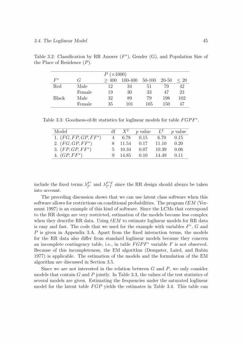
3.4. The Loglinear Model 45
Table 3.2: Classification by RR Answer (F ∗), Gender (G), and Population Size ofthe Place of Residence (P ).
P (×1000)F ∗ G ≥ 400 100-400 50-100 20-50 ≤ 20Red Male 12 34 51 79 42
Female 19 30 33 47 23Black Male 32 89 79 198 102
Female 35 101 105 150 47
Table 3.3: Goodness-of-fit statistics for loglinear models for table FGPF ∗.
Model df X2 p value L2 p value1. (FG,FP,GP, FF ∗) 4 6.78 0.15 6.70 0.152. (FG,GP, FF ∗) 8 11.54 0.17 11.10 0.203. (FP,GP, FF ∗) 5 10.34 0.07 10.39 0.064. (GP,FF ∗) 9 14.85 0.10 14.49 0.11
include the fixed terms λF ∗f∗ and λF ∗F
f∗f since the RR design should always be takeninto account.
The preceding discussion shows that we can use latent class software when thissoftware allows for restrictions on conditional probabilities. The program EM (Ver-munt 1997) is an example of this kind of software. Since the LCMs that correspondto the RR design are very restricted, estimation of the models become less complexwhen they describe RR data. Using EM to estimate loglinear models for RR datais easy and fast. The code that we used for the example with variables F ∗, G andP is given in Appendix 3.A. Apart from the fixed interaction terms, the modelsfor the RR data also differ from standard loglinear models because they concernan incomplete contingency table, i.e., in table FGPF ∗ variable F is not observed.Because of this incompleteness, the EM algorithm (Dempster, Laird, and Rubin1977) is applicable. The estimation of the models and the formulation of the EMalgorithm are discussed in Section 3.5.
Since we are not interested in the relation between G and P , we only considermodels that contain G and P jointly. In Table 3.3, the values of the test statistics ofseveral models are given. Estimating the frequencies under the saturated loglinearmodel for the latent table FGP yields the estimates in Table 3.4. This table can
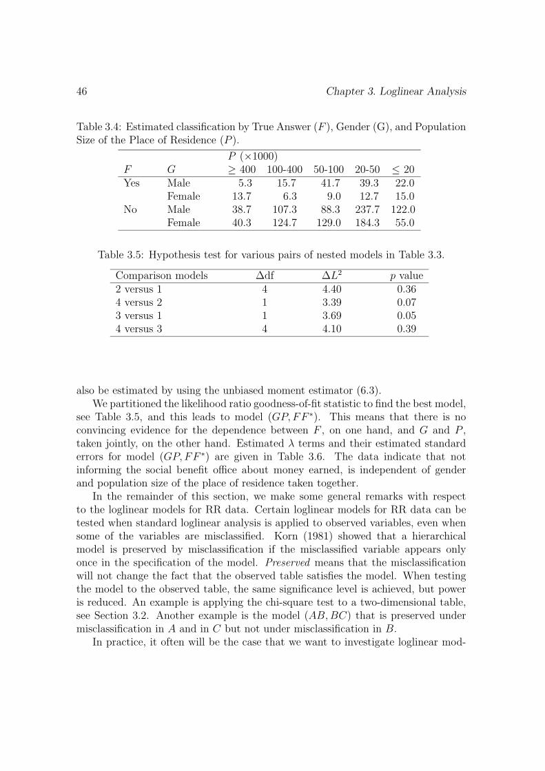
46 Chapter 3. Loglinear Analysis
Table 3.4: Estimated classification by True Answer (F ), Gender (G), and PopulationSize of the Place of Residence (P ).
P (×1000)F G ≥ 400 100-400 50-100 20-50 ≤ 20Yes Male 5.3 15.7 41.7 39.3 22.0
Female 13.7 6.3 9.0 12.7 15.0No Male 38.7 107.3 88.3 237.7 122.0
Female 40.3 124.7 129.0 184.3 55.0
Table 3.5: Hypothesis test for various pairs of nested models in Table 3.3.
Comparison models ∆df ∆L2 p value2 versus 1 4 4.40 0.364 versus 2 1 3.39 0.073 versus 1 1 3.69 0.054 versus 3 4 4.10 0.39
also be estimated by using the unbiased moment estimator (6.3).We partitioned the likelihood ratio goodness-of-fit statistic to find the best model,
see Table 3.5, and this leads to model (GP,FF ∗). This means that there is noconvincing evidence for the dependence between F , on one hand, and G and P ,taken jointly, on the other hand. Estimated λ terms and their estimated standarderrors for model (GP,FF ∗) are given in Table 3.6. The data indicate that notinforming the social benefit office about money earned, is independent of genderand population size of the place of residence taken together.
In the remainder of this section, we make some general remarks with respectto the loglinear models for RR data. Certain loglinear models for RR data can betested when standard loglinear analysis is applied to observed variables, even whensome of the variables are misclassified. Korn (1981) showed that a hierarchicalmodel is preserved by misclassification if the misclassified variable appears onlyonce in the specification of the model. Preserved means that the misclassificationwill not change the fact that the observed table satisfies the model. When testingthe model to the observed table, the same significance level is achieved, but poweris reduced. An example is applying the chi-square test to a two-dimensional table,see Section 3.2. Another example is the model (AB,BC) that is preserved undermisclassification in A and in C but not under misclassification in B.
In practice, it often will be the case that we want to investigate loglinear mod-
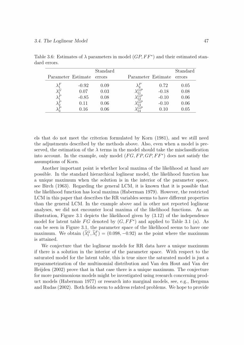
3.4. The Loglinear Model 47
Table 3.6: Estimates of λ parameters in model (GP,FF ∗) and their estimated stan-dard errors.
Parameter EstimateStandarderrors Parameter Estimate
Standarderrors
λF1 -0.92 0.09 λP
4 0.72 0.05λG
1 0.07 0.03 λGP11 -0.18 0.08
λP1 -0.85 0.08 λGP
12 -0.10 0.06λP
2 0.11 0.06 λGP13 -0.10 0.06
λP3 0.16 0.06 λGP
14 0.10 0.05
els that do not meet the criterion formulated by Korn (1981), and we still needthe adjustments described by the methods above. Also, even when a model is pre-served, the estimation of the λ terms in the model should take the misclassificationinto account. In the example, only model (FG,FP,GP, FF ∗) does not satisfy theassumptions of Korn.
Another important point is whether local maxima of the likelihood at hand arepossible. In the standard hierarchical loglinear model, the likelihood function hasa unique maximum when the solution is in the interior of the parameter space,see Birch (1963). Regarding the general LCM, it is known that it is possible thatthe likelihood function has local maxima (Haberman 1979). However, the restrictedLCM in this paper that describes the RR variables seems to have different propertiesthan the general LCM. In the example above and in other not reported loglinearanalyses, we did not encounter local maxima of the likelihood functions. As anillustration, Figure 3.1 depicts the likelihood given by (3.12) of the independencemodel for latent table FG denoted by (G,FF ∗) and applied to Table 3.1 (a). Ascan be seen in Figure 3.1, the parameter space of the likelihood seems to have onemaximum. We obtain (λG
1 , λF1 ) = (0.098,−0.92) as the point where the maximum
is attained.
We conjecture that the loglinear models for RR data have a unique maximumif there is a solution in the interior of the parameter space. With respect to thesaturated model for the latent table, this is true since the saturated model is just areparametrization of the multinomial distribution and Van den Hout and Van derHeijden (2002) prove that in that case there is a unique maximum. The conjecturefor more parsimonious models might be investigated using research concerning prod-uct models (Haberman 1977) or research into marginal models, see, e.g., Bergsmaand Rudas (2002). Both fields seem to address related problems. We hope to provide
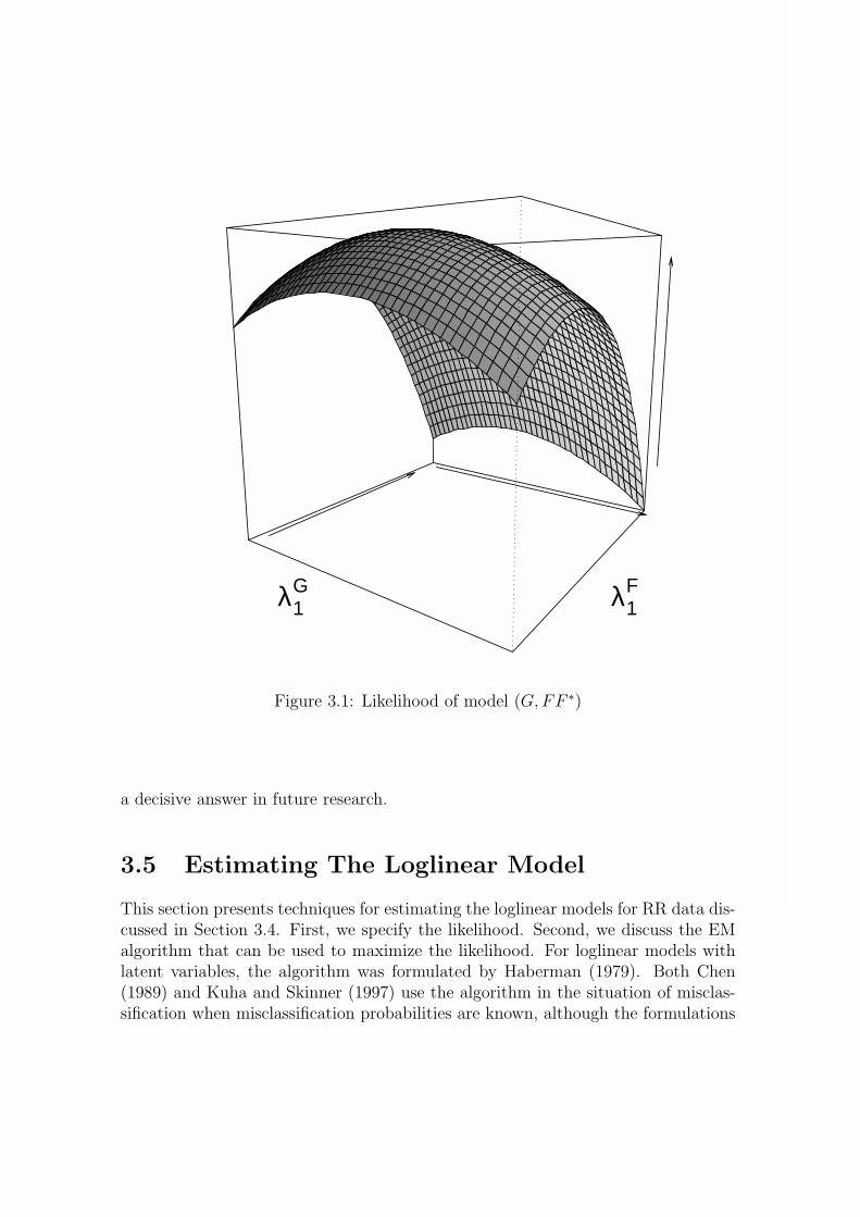
48 Chapter 3. Loglinear Analysis
λ1Fλ1
G
Figure 3.1: Likelihood of model (G,FF ∗)
a decisive answer in future research.
3.5 Estimating The Loglinear Model
This section presents techniques for estimating the loglinear models for RR data dis-cussed in Section 3.4. First, we specify the likelihood. Second, we discuss the EMalgorithm that can be used to maximize the likelihood. For loglinear models withlatent variables, the algorithm was formulated by Haberman (1979). Both Chen(1989) and Kuha and Skinner (1997) use the algorithm in the situation of misclas-sification when misclassification probabilities are known, although the formulations
3.5. Estimating The Loglinear Model 49
of the algorithm differ. Chen (1989) explicitly discusses RR data. We will reviewthe two formulations since the difference is important when a boundary solution isencountered. By a boundary solution, we mean an estimated expected cell frequencyin the latent table that equals zero. Section 3.6 will give examples of RR data whereboundary solutions occur.
To give the general formula of the likelihood, let the latent frequencies n =(n1, ..., nD)t be multinomially distributed with parameters N and θ = (θ1, ..., θD)t.We specify loglinear models by ηd = log θd, d ∈ 1, ..., D, and η = Mλ, whereη = (η1, ..., ηD)t, M is the D × r design matrix that defines the loglinear model,and λ = (λ1, ..., λr)
t is the parameter vector of the model. Ignoring constants, thelikelihood is given by
L(λ|n∗) =D∏
i=1
(θ∗i )n∗
i = expD∑
i=1
n∗i log(pi1e
η1 + .. + piDeηD), (3.11)
where n∗ is the vector with observed frequencies, and pij, i, j ∈ 1, ..., D, are theentries of the transition matrix that describe the misclassification with respect toθ. Since n is assumed to be multinomially distributed, n∗ is also multinomiallydistributed due to the specific form of the transition matrix (Van den Hout and Vander Heijden 2002, Section 5).
As an example, consider the likelihood of the independence model (G,F ) appliedto Table 3.1 (a), given by
L(λ|n∗) =4∏
i=1
(θ∗i )n∗
i = exp4∑
i=1
n∗i log(pi1e
η1 + pi2eη2 + pi3e
η3 + pi4eη4), (3.12)
where n∗ are the frequencies in Table 3.1 (a); pij, i, j ∈ 1, ..., 4, are the entries inP GF given by (3.7); and the non-redundant parameters are λG
1 and λF1 . Note that
parameter λ0 is not a free parameter in the loglinear model −− in this case
λ0 = − log∑gf
exp(λGg + λF
f ),
where g, f ∈ 1, 2.We can maximize (4.6) directly using the Newton-Raphson method, but we can
also maximize it using an EM algorithm. The program EM (Vermunt 1997) usesboth procedures. The program starts with an EM algorithm and uses Newton-Raphson when close to the maximum. The applicability of the EM algorithm to RRdata becomes clear when RR data are viewed as incomplete data. For each respon-dent, we can associate with the observed value of F ∗ the not-observed nonperturbed
50 Chapter 3. Loglinear Analysis
value of F . Together, these pairs form an incomplete data matrix. In the frameworkof Rubin (1976): The missing data are missing at random since they are missing bydesign.
Next we review the formulations of the EM algorithm given by Chen (1989) andKuha and Skinner (1997). We use the example in the preceding section and startwith the formulation by Chen (1989). Say we want to fit model (FGP, FF ∗). Withv = 0, 1, 2... denoting the cycles, the algorithm is given by
Initial estimate: m(0)fgp
E-step: n(v)f∗gpf = nf∗gp
(m
(v)fgpπf∗|f
)/(∑2t=1 m
(v)tgpπf∗|t
)M-step: Fit (FGP, FF ∗) to n
(v)f∗gpf and use estimated
expected frequencies to compute m(v+1)fgp ,
where m(0)fgp is the initial estimate of the frequencies in latent table FGP , nf∗gp
are the observed frequencies in the F ∗GP table, and in each step f ∗, g, f ∈ 1, 2,p ∈ 1, .., 5. The conditional probabilities πf∗|f are fixed and provided for by thetransition matrix for F given by (3.2).
To test the model after convergence, compare m(∞)f∗gp+ with nf∗gp using, for in-
stance, the chi-square test or the likelihood ratio test. The degrees of freedom ofthe chi-square distributions of these test statistics are the number of cells that arecompared minus the number of parameters fitted. For model (FGP, FF ∗), we have20 - 20 = 0 degrees of freedom since the λF ∗
f∗ and λF ∗Ff∗f are fixed due to the RR
design.
Chen (1989) is not explicit with respect to the fixed λ -terms in models such as(FGP, FF ∗). We think that it is important to stress that when fitting a loglinearmodel in the M-step, one should check whether the restrictions due to the RR designare maintained. The relations between λ terms and conditional probabilities in ourexample are
πf∗|f =exp(λF ∗
f∗ + λF ∗Ff∗f )∑
f∗ exp(λF ∗f∗ + λF ∗F
f∗f ), (3.13)
where f ∗, f ∈ 0, 1, and the summation is over values f ∗ ∈ 0, 1, see, e.g., Heinen(1996, Chapter 2). The relation (3.13) is the same for more parsimonious models
3.5. Estimating The Loglinear Model 51
for the latent table FGP . Using (3.13), we obtain
λF ∗1 = −1/4
(log π2|1 − log π1|1 − log π1|2 + log π2|2
)= 0
λF ∗F11 = −1/4
(log π2|1 − log π1|1 + log π1|2 − log π2|2
)= 0.69. (3.14)
When fitting (FGP, FF ∗) in the M-step in a standard way without maintainingthe restrictions, λF ∗
1 and λF ∗F11 converge to the fixed values of λF ∗
1 and λF ∗F11 . However,
when there is a boundary solution, this may not be the case. In Section 3.6, we willgive examples of RR data with boundary solutions. When the restrictions are notmaintained, estimated expected frequencies m
(∞)f∗gp+ are wrong; consequently, the
value of the test statistic is wrong. This means that the formulation of the EMalgorithm in Chen (1989) does not always yield the EM algorithm that we want.
To apply the EM algorithm correctly −− that is, in such a way that it also yieldsthe right estimates in the case of boundary solutions −− there are two possibleadjustments. We will explain these two adjustments and show that they are oneand the same due to the Collapsibility Theorem. First, we can fit (FGP, FF ∗) in theM-step using the fixed values of λF ∗
f∗ and λF ∗Ff∗f , given by (3.14). The disadvantage
is that this is not completely standard loglinear analysis since we should take careof these restrictions in estimating expected frequencies.
Second, we can use the E-step and M-step as given in Kuha and Skinner (1997),who refer to Chen (1989) but nevertheless give a different formulation of the algo-rithm −− namely
E-step: n(v)f∗gpf = nf∗gp
(m
(v)fgpπf∗|f
)/(∑2t=1 m
(v)tgpπf∗|t
)n
(v)fgp = n
(v)+gpf
M-step: Fit (FGP ) to n(v)fgp to obtain estimated
expected frequencies m(v+1)fgp .
The advantage is that the M-step is standard. With respect to the testing of themodel after convergence, Kuha and Skinner (1997) do not explicitly give a procedure,but we suggest doing the following. Structure the estimated frequencies mfgp in thethree-dimensional latent table FGP as a one-dimensional table of a compoundedvariable −− say m −− and compute the fitted frequencies under this model, denoted
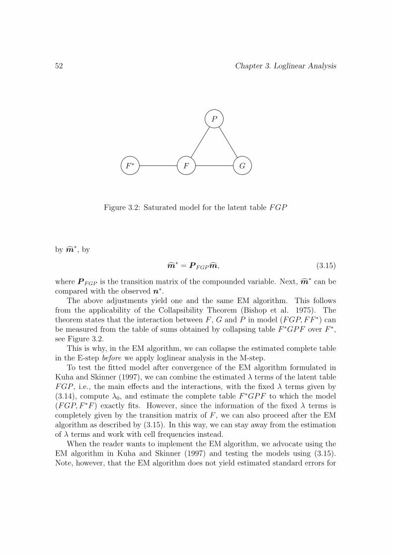
52 Chapter 3. Loglinear Analysis
F ∗ F G
P
Figure 3.2: Saturated model for the latent table FGP
by m∗, by
m∗ = P FGP m, (3.15)
where P FGP is the transition matrix of the compounded variable. Next, m∗ can becompared with the observed n∗.
The above adjustments yield one and the same EM algorithm. This followsfrom the applicability of the Collapsibility Theorem (Bishop et al. 1975). Thetheorem states that the interaction between F , G and P in model (FGP, FF ∗) canbe measured from the table of sums obtained by collapsing table F ∗GPF over F ∗,see Figure 3.2.
This is why, in the EM algorithm, we can collapse the estimated complete tablein the E-step before we apply loglinear analysis in the M-step.
To test the fitted model after convergence of the EM algorithm formulated inKuha and Skinner (1997), we can combine the estimated λ terms of the latent tableFGP , i.e., the main effects and the interactions, with the fixed λ terms given by(3.14), compute λ0, and estimate the complete table F ∗GPF to which the model(FGP, F ∗F ) exactly fits. However, since the information of the fixed λ terms iscompletely given by the transition matrix of F , we can also proceed after the EMalgorithm as described by (3.15). In this way, we can stay away from the estimationof λ terms and work with cell frequencies instead.
When the reader wants to implement the EM algorithm, we advocate using theEM algorithm in Kuha and Skinner (1997) and testing the models using (3.15).Note, however, that the EM algorithm does not yield estimated standard errors for
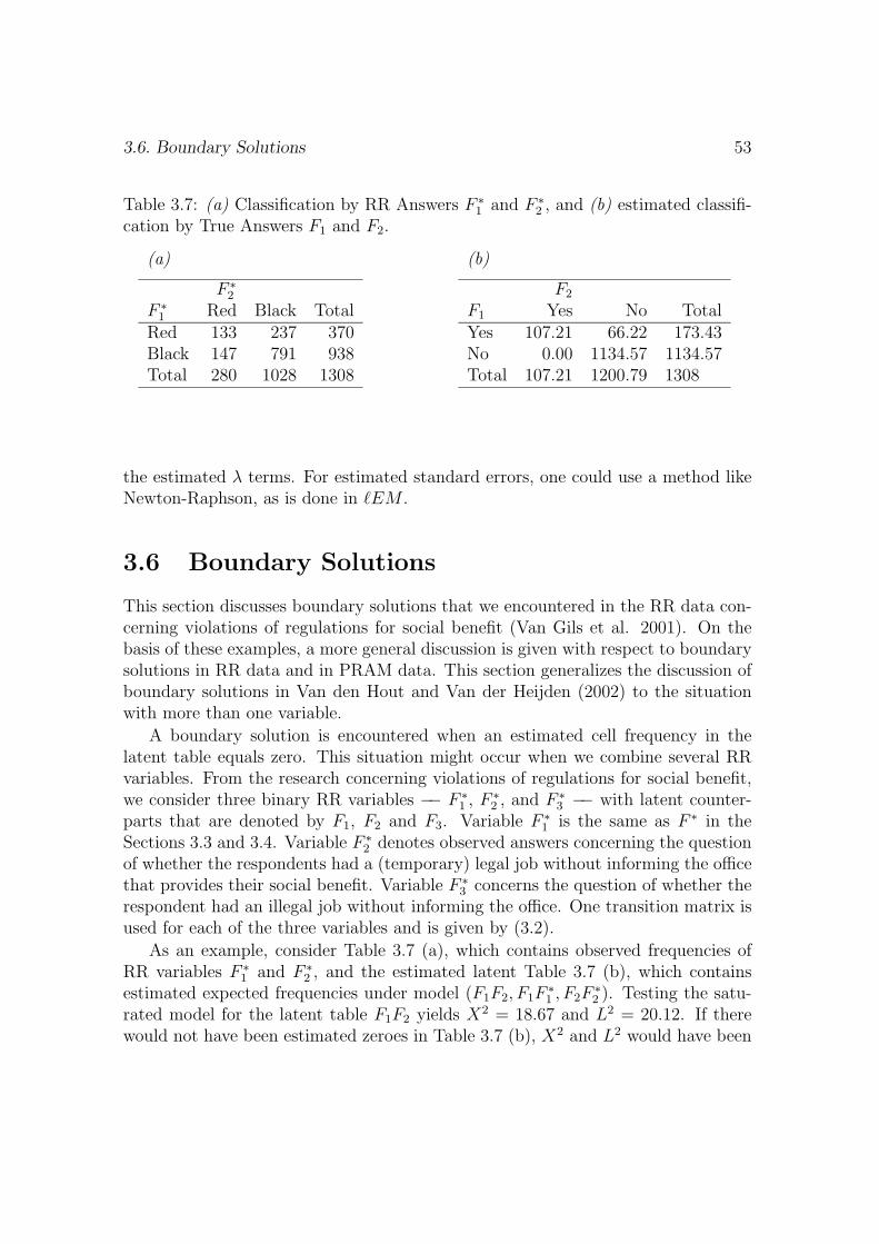
3.6. Boundary Solutions 53
Table 3.7: (a) Classification by RR Answers F ∗1 and F ∗
2 , and (b) estimated classifi-cation by True Answers F1 and F2.
(a)
F ∗2
F ∗1 Red Black Total
Red 133 237 370Black 147 791 938Total 280 1028 1308
(b)
F2
F1 Yes No TotalYes 107.21 66.22 173.43No 0.00 1134.57 1134.57Total 107.21 1200.79 1308
the estimated λ terms. For estimated standard errors, one could use a method likeNewton-Raphson, as is done in EM .
3.6 Boundary Solutions
This section discusses boundary solutions that we encountered in the RR data con-cerning violations of regulations for social benefit (Van Gils et al. 2001). On thebasis of these examples, a more general discussion is given with respect to boundarysolutions in RR data and in PRAM data. This section generalizes the discussion ofboundary solutions in Van den Hout and Van der Heijden (2002) to the situationwith more than one variable.
A boundary solution is encountered when an estimated cell frequency in thelatent table equals zero. This situation might occur when we combine several RRvariables. From the research concerning violations of regulations for social benefit,we consider three binary RR variables −− F ∗
1 , F ∗2 , and F ∗
3 −− with latent counter-parts that are denoted by F1, F2 and F3. Variable F ∗
1 is the same as F ∗ in theSections 3.3 and 3.4. Variable F ∗
2 denotes observed answers concerning the questionof whether the respondents had a (temporary) legal job without informing the officethat provides their social benefit. Variable F ∗
3 concerns the question of whether therespondent had an illegal job without informing the office. One transition matrix isused for each of the three variables and is given by (3.2).
As an example, consider Table 3.7 (a), which contains observed frequencies ofRR variables F ∗
1 and F ∗2 , and the estimated latent Table 3.7 (b), which contains
estimated expected frequencies under model (F1F2, F1F∗1 , F2F
∗2 ). Testing the satu-
rated model for the latent table F1F2 yields X2 = 18.67 and L2 = 20.12. If therewould not have been estimated zeroes in Table 3.7 (b), X2 and L2 would have been
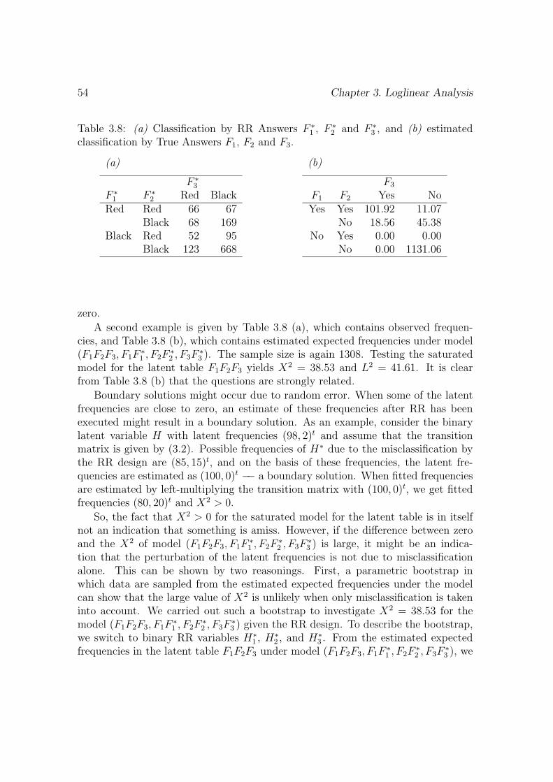
54 Chapter 3. Loglinear Analysis
Table 3.8: (a) Classification by RR Answers F ∗1 , F ∗
2 and F ∗3 , and (b) estimated
classification by True Answers F1, F2 and F3.
(a)
F ∗3
F ∗1 F ∗
2 Red BlackRed Red 66 67
Black 68 169Black Red 52 95
Black 123 668
(b)
F3
F1 F2 Yes NoYes Yes 101.92 11.07
No 18.56 45.38No Yes 0.00 0.00
No 0.00 1131.06
zero.
A second example is given by Table 3.8 (a), which contains observed frequen-cies, and Table 3.8 (b), which contains estimated expected frequencies under model(F1F2F3, F1F
∗1 , F2F
∗2 , F3F
∗3 ). The sample size is again 1308. Testing the saturated
model for the latent table F1F2F3 yields X2 = 38.53 and L2 = 41.61. It is clearfrom Table 3.8 (b) that the questions are strongly related.
Boundary solutions might occur due to random error. When some of the latentfrequencies are close to zero, an estimate of these frequencies after RR has beenexecuted might result in a boundary solution. As an example, consider the binarylatent variable H with latent frequencies (98, 2)t and assume that the transitionmatrix is given by (3.2). Possible frequencies of H∗ due to the misclassification bythe RR design are (85, 15)t, and on the basis of these frequencies, the latent fre-quencies are estimated as (100, 0)t −− a boundary solution. When fitted frequenciesare estimated by left-multiplying the transition matrix with (100, 0)t, we get fittedfrequencies (80, 20)t and X2 > 0.
So, the fact that X2 > 0 for the saturated model for the latent table is in itselfnot an indication that something is amiss. However, if the difference between zeroand the X2 of model (F1F2F3, F1F
∗1 , F2F
∗2 , F3F
∗3 ) is large, it might be an indica-
tion that the perturbation of the latent frequencies is not due to misclassificationalone. This can be shown by two reasonings. First, a parametric bootstrap inwhich data are sampled from the estimated expected frequencies under the modelcan show that the large value of X2 is unlikely when only misclassification is takeninto account. We carried out such a bootstrap to investigate X2 = 38.53 for themodel (F1F2F3, F1F
∗1 , F2F
∗2 , F3F
∗3 ) given the RR design. To describe the bootstrap,
we switch to binary RR variables H∗1 , H∗
2 , and H∗3 . From the estimated expected
frequencies in the latent table F1F2F3 under model (F1F2F3, F1F∗1 , F2F
∗2 , F3F
∗3 ), we
3.6. Boundary Solutions 55
sampled 100 tables H1H2H3 and next simulated 100 tables H∗1H
∗2H
∗3 using the RR
design. For each of these tables H∗1H
∗2H
∗3 the test statistic X2 is computed. The
mean value of the 100 simulated X2’s is 2.00, and the maximum is 9.25. This max-imum is not even close to the X2 = 38.53 of model (F1F2F3, F1F
∗1 , F2F
∗2 , F3F
∗3 ).
Results for the likelihood ratio test L2 are very similar.A second way to investigate whether the RR data can be described by mis-
classification alone is the following. Continuing with the example: Assume thatnone of the respondents committed fraud, or in other words, that the latent scoreis 2 for each variable F1, F2, and F3. Under this assumption, the expected num-ber of respondents with observed score black for each variable F ∗
1 , F ∗2 , and F ∗
3 is(8/10)3 × 1308 = 669.70. The observed number in the survey is 668. This mightsuggest that the assumption is correct and that there are no frauds at all in thesurvey. However, this is contradicted by the 66 respondents who have the scorered for each variable F ∗
1 , F ∗2 , and F ∗
3 −− a frequency that is much higher than theexpected (2/10)3 × 1308 = 10.46 under the assumption of no fraud at all.
The two reasonings show that, given the RR design in the research and theestimated expected frequencies in Table 3.8 (b), it is rather unlikely that Table 3.8(a) is the observed table. However, since the observed data are the starting pointof statistical inference, we should state the conclusion the other way around: GivenTable 3.8 (a) and the RR design, Table 3.8 (b) is probably not a good estimateof the latent frequencies. The cause for this estimation problem is probably thatsome respondents do not always follow the RR design and answer black too often,irrespective of the question asked. A reason for this might be that some respondentsdo not trust the privacy protection offered by the RR design and answer black sinceblack is associated with no. These respondents bring about a second perturbationof the latent frequencies besides the misclassification due to the RR design. In theconclusion, we will return to this problem.
To make the discussion more general, note that when the statistical disclosuremethod PRAM is applied, X2 > 0 for the saturated model for the latent tablecan only occur due to random error since the misclassification is executed by thecomputer. Also, in the case where RR data are not unlikely in the sense as discussedabove, a method is needed to deal with the fact that X2 might be unequal to zero.In the related field of incomplete data it also may occur that X2
0 > 0 (Schafer 1997).We suggest following Schafer (1997), who proposes taking the deviation from thenull as a baseline for assessing nonsaturated models and defines an adjusted teststatistic
X2adj = X2 − X2
0 ,
where X20 is the X2 of the saturated model. The likelihood ratio test is adjusted in
56 Chapter 3. Loglinear Analysis
the same way. The behavior of this adjusted test might be studied using Gelman,Meng and Stern (1996), who use Bayesian analysis to assess model fit in situationswhen X2 > 0 but when X2 is expected to be zero if the model is true.
3.7 Conclusion
This paper discusses loglinear analysis of randomized response data. It is shownthat this kind of analysis can be executed using existing latent class software.
The RR data from the example in this paper are difficult data. The problem isnot the theoretic misclassification due to the RR design since this paper shows thatwe can handle this misclassification. The problem is that some respondents do notfollow the RR design and −− of course −− that we cannot identify these ”cheaters”.To some extent we can use X2
0 , i.e., the test statistic for the saturated model for thelatent table, as a measure of the bias of the RR data but it provides not a decisiveanswer.
Asking sensitive questions will always produce incomplete or biased data. So onemust make do with what one has got, and our idea is that RR performs relatively well(Van der Heijden, Van Gils, Bouts, and Hox 2000). Analysis of RR data in the futuremight profit from research into more methodological aspects of RR designs, seeBoeije and Lensvelt-Mulders (2002), who discuss cheating in RR designs. A possibleform of cheating is when a respondent answers black, irrespective of the questionasked since he or she does not trust the privacy protection. When respondentsunderstand the privacy protection offered by the RR design better, data might beless biased. Another approach might be to add extra parameters to the model inorder to describe cheating behavior. This is not straightforward since it is difficultto model cheating behavior, and also we might run into identifiability problems, see,e.g., Goodman (1974).
The question of how the bias in the data influences the analysis is difficult to an-swer. Obvious is that results should be interpret with care and that cross-classifyingseveral RR questions might increase the bias of the results. We suggest the follow-ing: When the saturated model fits perfectly, i.e., X2
0 = 0, we advocate the loglinearmodeling as described in Section 3.4. When X2
0 > 0, one should be more careful,and the reasonings used in Section 3.6 can be used to assess bias in the RR data dueto the ”cheaters”. When the parametric bootstrap in Section 3.6 makes the value ofX2
0 unlikely, it is unclear how to interpret the results of the loglinear analysis. WhenX2
0 is not too large, i.e., the deviation from the null can be explained by randomerror, an adjusted test statistic can be used to test the fitting of loglinear models.
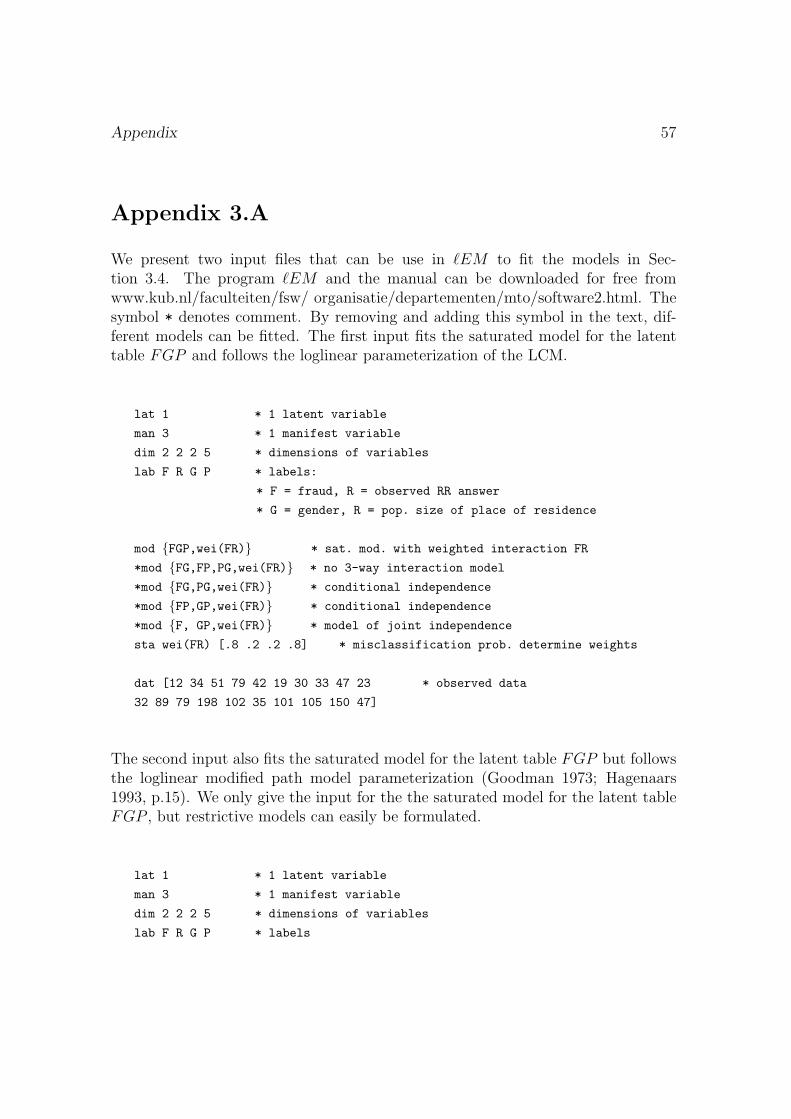
Appendix 57
Appendix 3.A
We present two input files that can be use in EM to fit the models in Sec-tion 3.4. The program EM and the manual can be downloaded for free fromwww.kub.nl/faculteiten/fsw/ organisatie/departementen/mto/software2.html. Thesymbol * denotes comment. By removing and adding this symbol in the text, dif-ferent models can be fitted. The first input fits the saturated model for the latenttable FGP and follows the loglinear parameterization of the LCM.
lat 1 * 1 latent variable
man 3 * 1 manifest variable
dim 2 2 2 5 * dimensions of variables
lab F R G P * labels:
* F = fraud, R = observed RR answer
* G = gender, R = pop. size of place of residence
mod FGP,wei(FR) * sat. mod. with weighted interaction FR
*mod FG,FP,PG,wei(FR) * no 3-way interaction model
*mod FG,PG,wei(FR) * conditional independence
*mod FP,GP,wei(FR) * conditional independence
*mod F, GP,wei(FR) * model of joint independence
sta wei(FR) [.8 .2 .2 .8] * misclassification prob. determine weights
dat [12 34 51 79 42 19 30 33 47 23 * observed data
32 89 79 198 102 35 101 105 150 47]
The second input also fits the saturated model for the latent table FGP but followsthe loglinear modified path model parameterization (Goodman 1973; Hagenaars1993, p.15). We only give the input for the the saturated model for the latent tableFGP , but restrictive models can easily be formulated.
lat 1 * 1 latent variable
man 3 * 1 manifest variable
dim 2 2 2 5 * dimensions of variables
lab F R G P * labels

58
mod FGP FGP * saturated model
R|F wei(RF) * specifying weights
sta wei(RF) [.8 .2 .2 .8] * using misclassification probabilities
dat [12 34 51 79 42 19 30 33 47 23 * observed data
32 89 79 198 102 35 101 105 150 47]

Chapter 4
Randomized Response in a 2 × 2Factorial Design
4.1 Introduction
Randomized response (RR) is an interview technique that can be used when sensitivequestions have to be asked (Warner 1965; Chaudhuri and Mukerjee 1988). Examplesof sensitive questions are questions about alcohol consumption, sexual behavior orfraud. Respondents might be reluctant to answer sensitive questions directly. RRtechniques have in common that the true status of the individual respondent is notrevealed since his observed answer depends not only on his status but also on aspecified probability mechanism.
As an example, assume that the sensitive question is whether the respondent hascommitted fraud. The RR technique introduced by Boruch (1971), the force responsemethod, goes as follows. After the sensitive question is asked, the respondent throwstwo dice and keeps the outcome hidden from the interviewer. If the outcome of thedice is 2, 3 or 4, the respondent answers yes. If the outcome 5, 6, 7, 8, 9 or 10,he answers according to the truth. If the outcome 11 or 12, he answers no. Theobserved answer depends both on the true status of the respondent and on the diceas the probability mechanism. Due to the use of the probability mechanism, theprivacy of the individual respondent is guaranteed. RR techniques have been appliedin the Netherlands (Van Gils, Van der Heijden, Laudy, and Ross 2003; Elffers, Vander Heijden, and Hezemans 2003).
Chen (1989) used the concept of misclassification to describe RR data that arecollected using the RR design by Warner (1965). With each RR variable a transitionmatrix is associated that contains conditional misclassification probabilities. When
59
60 Chapter 4. Randomized Response in a 2 × 2 Factorial Design
the true status regarding the sensitive question is modeled by the discrete stochasticvariable X with sample space 1, 2, ..., J, only the misclassified values of X areobserved. The misclassified version of X is denoted X∗ and it has the same samplespace as X. The distribution of X∗ is the J-component finite mixture given by
IP (X∗ = i) =J∑
j=1
IP (X∗ = i|X = j)IP (A = j), (4.1)
where i = 1, ..., J , and IP (X∗ = i|X = j) for all i, j ∈ 1, 2, ..., J are fixed andgiven by the transition matrix of X.
The basis for this paper is a survey where some respondents were asked sensitivequestions about fraudulent behavior directly and others were asked the same ques-tions using RR. The RR was performed using the forced response method. Besidesthe use of RR as a factor, the use of a PC was a second factor, i.e., some respondentswere asked sensitive questions using a PC and others were asked the same questionswithout the use of a PC. Research questions concern the association between fraudand the PC/RR-classification. For instance, is fraud more easily admitted when RRis used?
Due to the fact that the use of RR induces a misclassification, standard statisticalmodels cannot be used since they do not take into account the misclassification. Thispaper discusses the adjustment of the standard loglinear model so that the modelcan deal with the particulars of the current survey. The approach consists of twosteps. First, the paper shows that the forced response method can be described usinga transition matrix with conditional misclassification probabilities. Understandingthe forced response method as a misclassification design generalizes for instancethe two formulations of the likelihood of the logistic regression model for RR datain Van der Heijden and Van Gils (1996). Second, the paper shows that, with anadaptation regarding the misclassification, the current survey can be analyzed usingthe framework in Van den Hout and Van der Heijden (2004), in which the generalRR design is described by a restrictive latent class model. To illustrate the theory,the paper discusses an example. The example includes a power analysis for testingloglinear models for RR data. The power analysis is important since using RRcauses extra variability in the data and extra variability decreases power.
The outline of the paper is as follows. Section 4.2 introduces the survey. Section4.3 describes the forced response method as a misclassification design. Section 4.4discusses the estimation of loglinear models and shows how the design of the currentsurvey fits into the latent class framework. Section 4.5 illustrates the theory byanalyzing the RR data of the survey, and investigates the power of testing loglinear
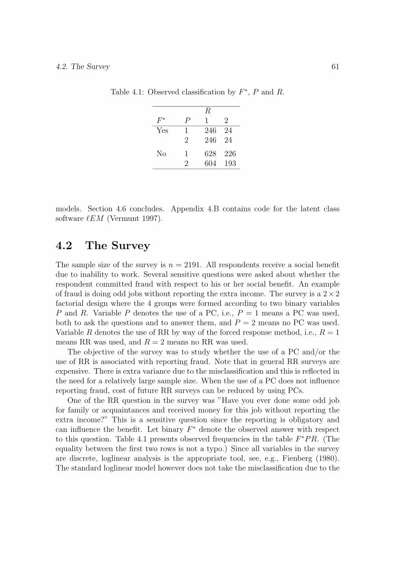
4.2. The Survey 61
Table 4.1: Observed classification by F ∗, P and R.
RF ∗ P 1 2Yes 1 246 24
2 246 24
No 1 628 2262 604 193
models. Section 4.6 concludes. Appendix 4.B contains code for the latent classsoftware EM (Vermunt 1997).
4.2 The Survey
The sample size of the survey is n = 2191. All respondents receive a social benefitdue to inability to work. Several sensitive questions were asked about whether therespondent committed fraud with respect to his or her social benefit. An exampleof fraud is doing odd jobs without reporting the extra income. The survey is a 2×2factorial design where the 4 groups were formed according to two binary variablesP and R. Variable P denotes the use of a PC, i.e., P = 1 means a PC was used,both to ask the questions and to answer them, and P = 2 means no PC was used.Variable R denotes the use of RR by way of the forced response method, i.e., R = 1means RR was used, and R = 2 means no RR was used.
The objective of the survey was to study whether the use of a PC and/or theuse of RR is associated with reporting fraud. Note that in general RR surveys areexpensive. There is extra variance due to the misclassification and this is reflected inthe need for a relatively large sample size. When the use of a PC does not influencereporting fraud, cost of future RR surveys can be reduced by using PCs.
One of the RR question in the survey was ”Have you ever done some odd jobfor family or acquaintances and received money for this job without reporting theextra income?” This is a sensitive question since the reporting is obligatory andcan influence the benefit. Let binary F ∗ denote the observed answer with respectto this question. Table 4.1 presents observed frequencies in the table F ∗PR. (Theequality between the first two rows is not a typo.) Since all variables in the surveyare discrete, loglinear analysis is the appropriate tool, see, e.g., Fienberg (1980).The standard loglinear model however does not take the misclassification due to the
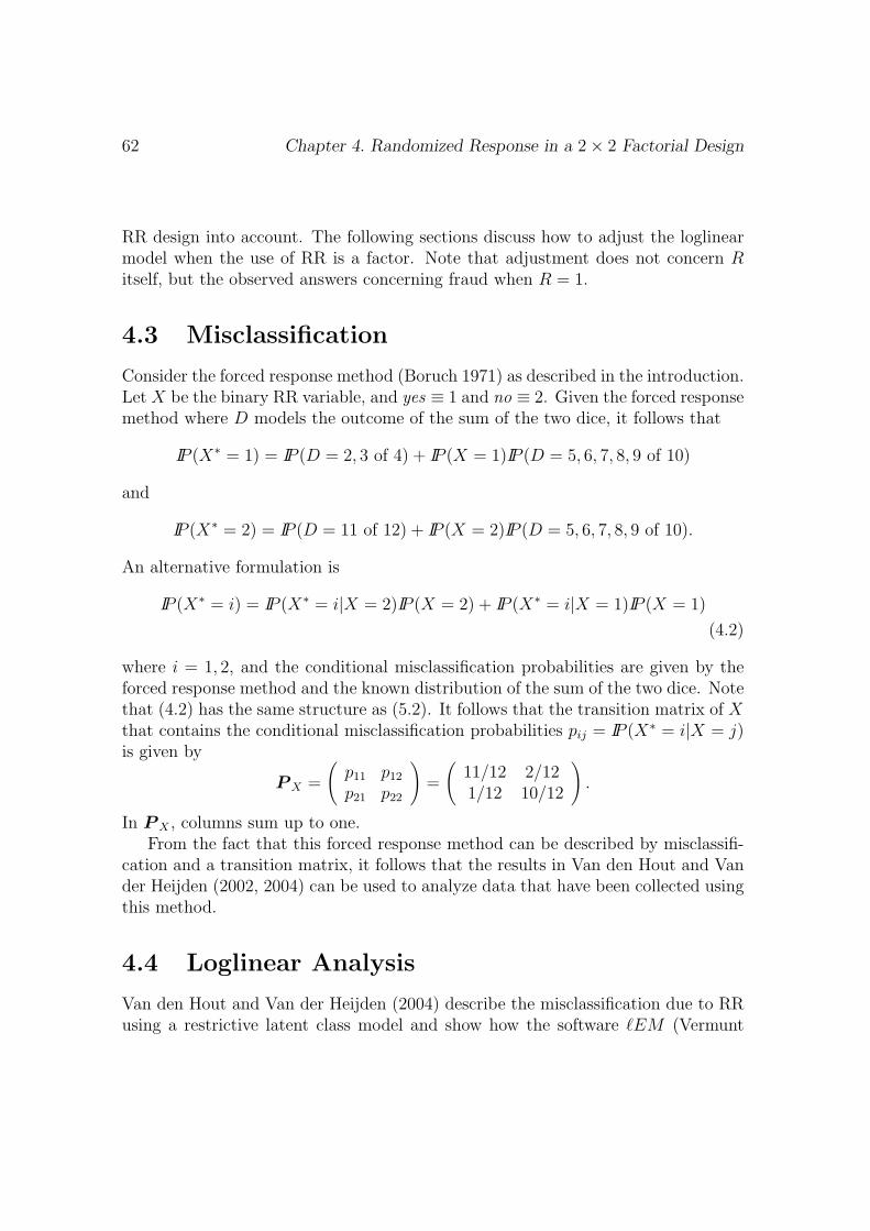
62 Chapter 4. Randomized Response in a 2 × 2 Factorial Design
RR design into account. The following sections discuss how to adjust the loglinearmodel when the use of RR is a factor. Note that adjustment does not concern Ritself, but the observed answers concerning fraud when R = 1.
4.3 Misclassification
Consider the forced response method (Boruch 1971) as described in the introduction.Let X be the binary RR variable, and yes ≡ 1 and no ≡ 2. Given the forced responsemethod where D models the outcome of the sum of the two dice, it follows that
IP (X∗ = 1) = IP (D = 2, 3 of 4) + IP (X = 1)IP (D = 5, 6, 7, 8, 9 of 10)
and
IP (X∗ = 2) = IP (D = 11 of 12) + IP (X = 2)IP (D = 5, 6, 7, 8, 9 of 10).
An alternative formulation is
IP (X∗ = i) = IP (X∗ = i|X = 2)IP (X = 2) + IP (X∗ = i|X = 1)IP (X = 1)
(4.2)
where i = 1, 2, and the conditional misclassification probabilities are given by theforced response method and the known distribution of the sum of the two dice. Notethat (4.2) has the same structure as (5.2). It follows that the transition matrix of Xthat contains the conditional misclassification probabilities pij = IP (X∗ = i|X = j)is given by
P X =
(p11 p12
p21 p22
)=
(11/12 2/121/12 10/12
).
In P X , columns sum up to one.From the fact that this forced response method can be described by misclassifi-
cation and a transition matrix, it follows that the results in Van den Hout and Vander Heijden (2002, 2004) can be used to analyze data that have been collected usingthis method.
4.4 Loglinear Analysis
Van den Hout and Van der Heijden (2004) describe the misclassification due to RRusing a restrictive latent class model and show how the software EM (Vermunt
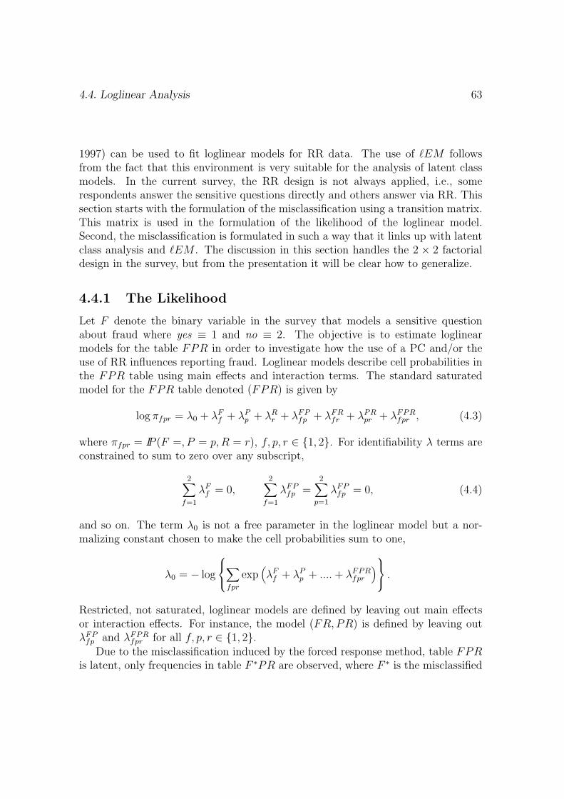
4.4. Loglinear Analysis 63
1997) can be used to fit loglinear models for RR data. The use of EM followsfrom the fact that this environment is very suitable for the analysis of latent classmodels. In the current survey, the RR design is not always applied, i.e., somerespondents answer the sensitive questions directly and others answer via RR. Thissection starts with the formulation of the misclassification using a transition matrix.This matrix is used in the formulation of the likelihood of the loglinear model.Second, the misclassification is formulated in such a way that it links up with latentclass analysis and EM . The discussion in this section handles the 2 × 2 factorialdesign in the survey, but from the presentation it will be clear how to generalize.
4.4.1 The Likelihood
Let F denote the binary variable in the survey that models a sensitive questionabout fraud where yes ≡ 1 and no ≡ 2. The objective is to estimate loglinearmodels for the table FPR in order to investigate how the use of a PC and/or theuse of RR influences reporting fraud. Loglinear models describe cell probabilities inthe FPR table using main effects and interaction terms. The standard saturatedmodel for the FPR table denoted (FPR) is given by
log πfpr = λ0 + λFf + λP
p + λRr + λFP
fp + λFRfr + λPR
pr + λFPRfpr , (4.3)
where πfpr = IP (F =, P = p,R = r), f, p, r ∈ 1, 2. For identifiability λ terms areconstrained to sum to zero over any subscript,
2∑f=1
λFf = 0,
2∑f=1
λFPfp =
2∑p=1
λFPfp = 0, (4.4)
and so on. The term λ0 is not a free parameter in the loglinear model but a nor-malizing constant chosen to make the cell probabilities sum to one,
λ0 = − log
∑fpr
exp(λF
f + λPp + .... + λFPR
fpr
) .
Restricted, not saturated, loglinear models are defined by leaving out main effectsor interaction effects. For instance, the model (FR,PR) is defined by leaving outλFP
fp and λFPRfpr for all f, p, r ∈ 1, 2.
Due to the misclassification induced by the forced response method, table FPRis latent, only frequencies in table F ∗PR are observed, where F ∗ is the misclassified
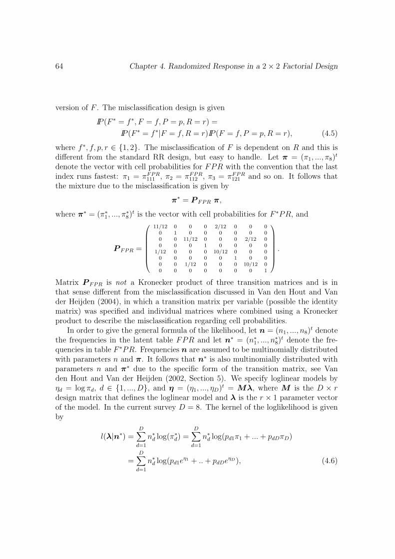
64 Chapter 4. Randomized Response in a 2 × 2 Factorial Design
version of F . The misclassification design is given
IP (F ∗ = f ∗, F = f, P = p,R = r) =
IP (F ∗ = f ∗|F = f,R = r)IP (F = f, P = p,R = r), (4.5)
where f ∗, f, p, r ∈ 1, 2. The misclassification of F is dependent on R and this isdifferent from the standard RR design, but easy to handle. Let π = (π1, ..., π8)
t
denote the vector with cell probabilities for FPR with the convention that the lastindex runs fastest: π1 = πFPR
111 , π2 = πFPR112 , π3 = πFPR
121 and so on. It follows thatthe mixture due to the misclassification is given by
π∗ = P FPR π,
where π∗ = (π∗1, ..., π
∗8)
t is the vector with cell probabilities for F ∗PR, and
P FPR =
11/12 0 0 0 2/12 0 0 00 1 0 0 0 0 0 00 0 11/12 0 0 0 2/12 00 0 0 1 0 0 0 0
1/12 0 0 0 10/12 0 0 00 0 0 0 0 1 0 00 0 1/12 0 0 0 10/12 00 0 0 0 0 0 0 1
.
Matrix P FPR is not a Kronecker product of three transition matrices and is inthat sense different from the misclassification discussed in Van den Hout and Vander Heijden (2004), in which a transition matrix per variable (possible the identitymatrix) was specified and individual matrices where combined using a Kroneckerproduct to describe the misclassification regarding cell probabilities.
In order to give the general formula of the likelihood, let n = (n1, ..., n8)t denote
the frequencies in the latent table FPR and let n∗ = (n∗1, ..., n
∗8)
t denote the fre-quencies in table F ∗PR. Frequencies n are assumed to be multinomially distributedwith parameters n and π. It follows that n∗ is also multinomially distributed withparameters n and π∗ due to the specific form of the transition matrix, see Vanden Hout and Van der Heijden (2002, Section 5). We specify loglinear models byηd = log πd, d ∈ 1, ..., D, and η = (η1, ..., ηD)t = Mλ, where M is the D × rdesign matrix that defines the loglinear model and λ is the r × 1 parameter vectorof the model. In the current survey D = 8. The kernel of the loglikelihood is givenby
l(λ|n∗) =D∑
d=1
n∗d log(π∗
d) =D∑
d=1
n∗d log(pd1π1 + ... + pdDπD)
=D∑
d=1
n∗d log(pd1e
η1 + .. + pdDeηD), (4.6)
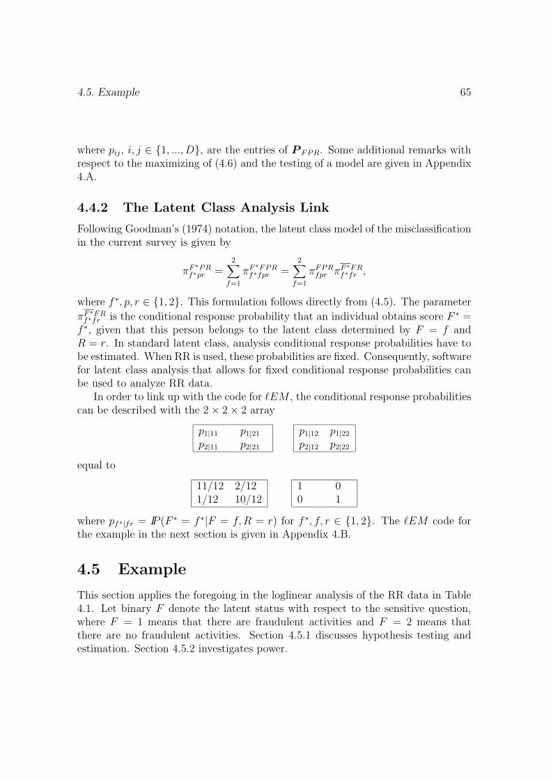
4.5. Example 65
where pij, i, j ∈ 1, ..., D, are the entries of P FPR. Some additional remarks withrespect to the maximizing of (4.6) and the testing of a model are given in Appendix4.A.
4.4.2 The Latent Class Analysis Link
Following Goodman’s (1974) notation, the latent class model of the misclassificationin the current survey is given by
πF ∗PRf∗pr =
2∑f=1
πF ∗FPRf∗fpr =
2∑f=1
πFPRfpr πF ∗FR
f∗fr ,
where f ∗, p, r ∈ 1, 2. This formulation follows directly from (4.5). The parameter
πF ∗FRf∗fr is the conditional response probability that an individual obtains score F ∗ =
f ∗, given that this person belongs to the latent class determined by F = f andR = r. In standard latent class, analysis conditional response probabilities have tobe estimated. When RR is used, these probabilities are fixed. Consequently, softwarefor latent class analysis that allows for fixed conditional response probabilities canbe used to analyze RR data.
In order to link up with the code for EM , the conditional response probabilitiescan be described with the 2 × 2 × 2 array
p1|11 p1|21
p2|11 p2|21
p1|12 p1|22
p2|12 p2|22
equal to
11/12 2/121/12 10/12
1 00 1
where pf∗|fr = IP (F ∗ = f ∗|F = f,R = r) for f ∗, f, r ∈ 1, 2. The EM code forthe example in the next section is given in Appendix 4.B.
4.5 Example
This section applies the foregoing in the loglinear analysis of the RR data in Table4.1. Let binary F denote the latent status with respect to the sensitive question,where F = 1 means that there are fraudulent activities and F = 2 means thatthere are no fraudulent activities. Section 4.5.1 discusses hypothesis testing andestimation. Section 4.5.2 investigates power.
66 Chapter 4. Randomized Response in a 2 × 2 Factorial Design
4.5.1 Hypothesis Testing and Estimation
Goodness-of-fit statistics for different loglinear models for latent table FPR are givenin Table 4.2, where X2 denotes the Pearson chi-square statistic and L2 denotes thelikelihood ratio statistic. Since the 2 × 2 factorial design is an experimental designwhere the 4 groups are formed using P and R, we must include the λPR
pr terms inall the models to be considered (Fienberg 1980, Chapter 6). In other words, weconsider only the loglinear models where the estimated expected marginal totals forP and R are equal to the observed totals fixed by design.
A goodness-of-fit statistic is used to test the current model against the alter-native of a saturated model. The L2 statistic can also be used to compare nestedmodels by partitioning the chi-square (Fienberg 1980, Section 4.3). When we choosesignificance level α equal to 0.10 and use the partitioning, we obtain (FR,PR) asthe best model for latent table FPR (∆df=1, ∆L2 = 0.36, p = 0.55). In the nextsection the choice of α will be motivated.
Interpretation of (FR,PR): There is an association between reporting fraud andthe use of RR, but there is no association between reporting fraud and the use of acomputer. As before, let yes ≡ 1 and no ≡ 2. Probabilities π
F |PR1|pr = IP (F = 1|P =
p,R = r) for the 4 groups can be estimated using the fit of model (FR,PR). Weobtain
π1|11 = π1|21 =π121∑2
f=1 πf21
= 0.158
π1|12 = π1|22 = 0.103.
The estimates show that when RR is used, more fraud is reported.With respect to the interpretation, it is also possible to use a logit model instead
of a loglinear model (Fienberg 1980, Chapter 6). The logit model takes explicitlyinto account that one of the variables is a dependent variable. The estimated logitmodel presents the results of the estimated loglinear model in a different way. Thelogit model that corresponds with the loglinear model (FR,PR) is given by
log(πFPR
1pr
/πFPR
2pr
)= w + wR
r , (4.7)
where p, r ∈ 1, 2. The interpretation of the logit model is straightforward whenthe underlying loglinear model is made identifiable using dummy coding, i.e., theredundant λ terms are set to zero. In the loglinear model this means
λF2 = λP
2 = λR2 = λFR
12 = λFR21 = λFR
22 = λPR12 = λPR
21 = λPR22 = 0.
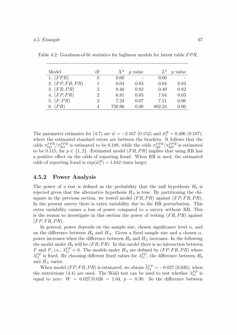
4.5. Example 67
Table 4.2: Goodness-of-fit statistics for loglinear models for latent table FPR.
Model df X2 p value L2 p value1. (FPR) 0 0.00 - 0.00 -2. (FP, FR, PR) 1 0.04 0.83 0.04 0.833. (FR,PR) 2 0.40 0.82 0.40 0.824. (FP, PR) 2 6.81 0.03 7.04 0.035. (F, PR) 3 7.23 0.07 7.51 0.066. (PR) 4 750.96 0.00 802.24 0.00
The parameter estimates for (4.7) are w = −2.167 (0.152) and wR1 = 0.496 (0.187),
where the estimated standard errors are between the brackets. It follows that theodds πFPR
1p1 /πFPR2p1 is estimated to be 0.188, while the odds πFPR
1p2 /πFPR2p2 is estimated
to be 0.115, for p ∈ 1, 2. Estimated model (FR,PR) implies that using RR hasa positive effect on the odds of reporting fraud. When RR is used, the estimatedodds of reporting fraud is exp(wR
1 ) = 1.642 times larger.
4.5.2 Power Analysis
The power of a test is defined as the probability that the null hypothesis H0 isrejected given that the alternative hypothesis HA is true. By partitioning the chi-square in the previous section, we tested model (FR,PR) against (FP, FR, PR).In the present survey there is extra variability due to the RR perturbation. Thisextra variability causes a loss of power compared to a survey without RR. Thisis the reason to investigate in this section the power of testing (FR,PR) against(FP, FR, PR).
In general, power depends on the sample size, chosen significance level α, andon the difference between H0 and HA. Given a fixed sample size and a chosen α,power increases when the difference between H0 and HA increases. In the followingthe model under H0 will be (FR,PR). In this model there is no interaction betweenF and P , i.e., λFP
11 = 0. The models under HA are defined by (FP, FR, PR) whereλFP
11 is fixed. By choosing different fixed values for λFP11 , the difference between H0
and HA varies.When model (FP, FR, PR) is estimated, we obtain λFP
11 = −0.027 (0.026), whenthe restrictions (4.4) are used. The Wald test can be used to test whether λFP
11 isequal to zero: W = 0.027/0.026 = 1.04, p = 0.30. So the difference between
68 Chapter 4. Randomized Response in a 2 × 2 Factorial Design
estimated models (FR,PR) and (FP, FR, PR) is small. Given this small differenceand the fact that power is increased when significance level α is increased, we chosesignificance level α = 0.10.
Simulation will be used to compute the power. Note that RR data are subjectto two stochastic processes: the survey sampling and the misclassification design.Both processes are taken into account in the simulation. Let the model under H0
be denoted M0 and the model under HA be denoted MA. One simulation goes asfollows.
1. Estimate expected frequencies m = (m1, ..., m8)t for latent table
FPR under MA
2. Draw a sample s from a multinomial distribution with parametersπ = m/n and n.
3. Simulate the RR design for s to obtain simulated frequencies oftable F ∗PR.
4. Fit M0 to simulated table F ∗PR and accept or reject M0 usingsignificance level α.
The proportion of times M0 is rejected by the goodness-of-fit test is the power oftesting M0 against MA, given a choice of α. As an illustration of the simulation, Fig-ure 4.1 shows the distribution of the 1000 times simulated goodness-of-fit statistic L2
when M0 = (FR,PR) and MA = (FP, FR, PR). The plotted line is the noncentralchi-square distribution with df = 2 and non-centrality parameter γ = 0.36. FromFigure 4.1 can be concluded that the simulated L2 follows the noncentral chi-squaredistribution, which is according to theory (compare Agresti 2002, Section 6.5.4.).
Next, the power of testing model (FR,PR) against alternative models (FP, FR,PR) with fixed λFP
11 is assessed. Figure 4.2 presents the simulated power curve forvarying choices of λFP
11 , where the goodness of fit is tested using L2. Note that whenλFP
11 = 0, (FR,PR) is tested against itself and the power equals α = 0.10. The blackcircle in Figure 4.2 indicates the power of testing (FR,PR) against (FP, FR, PR)when fixed λFP
11 is equal to λFP11 = −0.027.
From the simulation results it follows that there is adequate power (≥ 0.80) intesting (FR,PR) against (FP, FR, PR) when λFP
11 ≤ −0.13 or 0.13 ≤ λFP11 . Inter-
pretation of λFP11 is via exp(4λFP
11 ) which is the odds ratio between F and P (Fienberg1980, Section 2.5). In model (FR,PR), λFP
11 = 0 and the odds ratio is 1, i.e., thereis no association between F and P . From the power analysis above, it follows thatthere is adequate power (≥ 0.80) in testing (FR,PR) against (FP, FR, PR) whenthe odds ratio between F and P lies outside the interval (0.60,1.68).
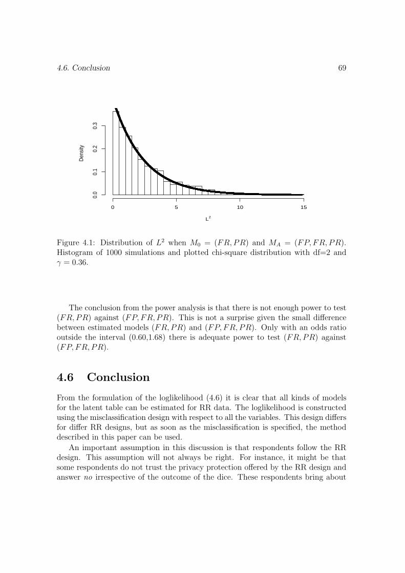
4.6. Conclusion 69
L2
Den
sity
0 5 10 15
0.0
0.1
0.2
0.3
Figure 4.1: Distribution of L2 when M0 = (FR,PR) and MA = (FP, FR, PR).Histogram of 1000 simulations and plotted chi-square distribution with df=2 andγ = 0.36.
The conclusion from the power analysis is that there is not enough power to test(FR,PR) against (FP, FR, PR). This is not a surprise given the small differencebetween estimated models (FR,PR) and (FP, FR, PR). Only with an odds ratiooutside the interval (0.60,1.68) there is adequate power to test (FR,PR) against(FP, FR, PR).
4.6 Conclusion
From the formulation of the loglikelihood (4.6) it is clear that all kinds of modelsfor the latent table can be estimated for RR data. The loglikelihood is constructedusing the misclassification design with respect to all the variables. This design differsfor differ RR designs, but as soon as the misclassification is specified, the methoddescribed in this paper can be used.
An important assumption in this discussion is that respondents follow the RRdesign. This assumption will not always be right. For instance, it might be thatsome respondents do not trust the privacy protection offered by the RR design andanswer no irrespective of the outcome of the dice. These respondents bring about
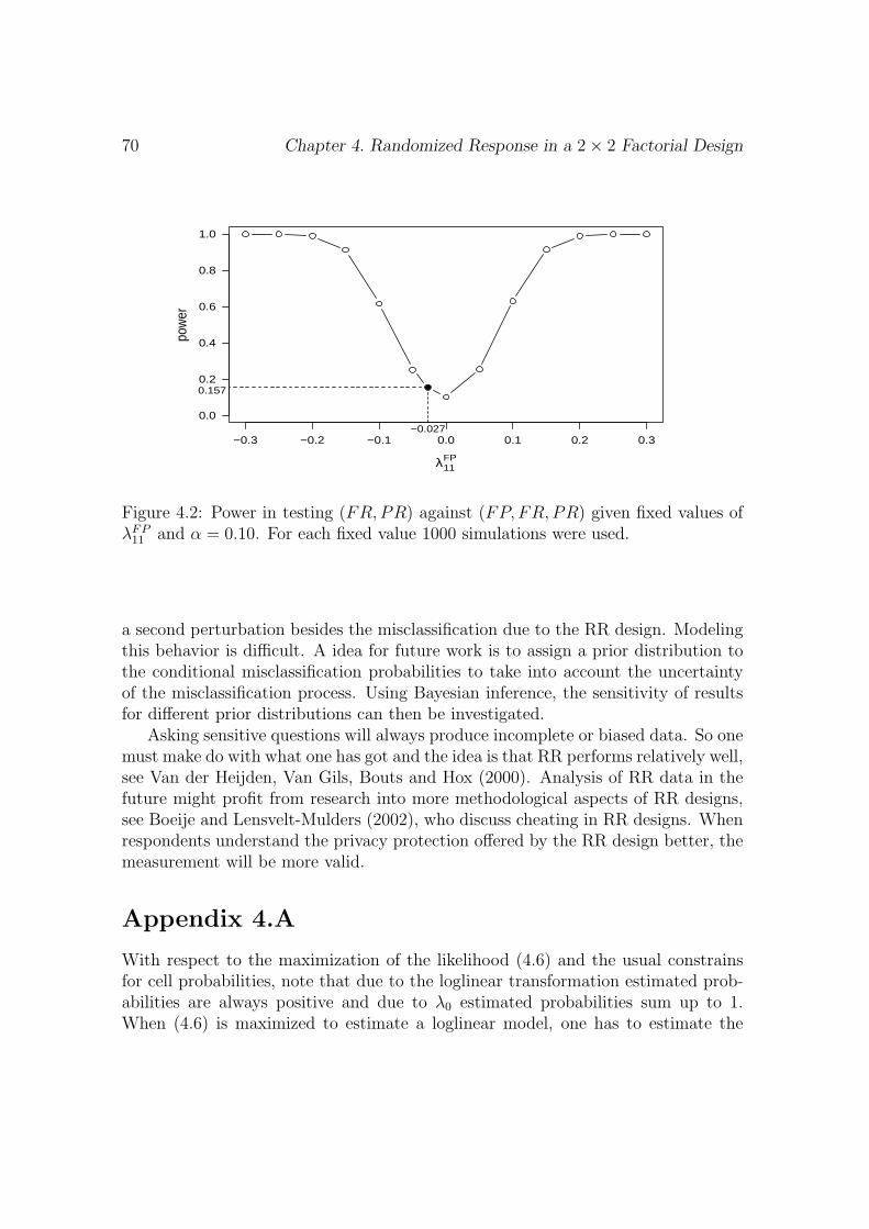
70 Chapter 4. Randomized Response in a 2 × 2 Factorial Design
−0.3 −0.2 −0.1 0.0 0.1 0.2 0.3
0.0
0.2
0.4
0.6
0.8
1.0
λ11FP
pow
er
−0.027
0.157
Figure 4.2: Power in testing (FR,PR) against (FP, FR, PR) given fixed values ofλFP
11 and α = 0.10. For each fixed value 1000 simulations were used.
a second perturbation besides the misclassification due to the RR design. Modelingthis behavior is difficult. A idea for future work is to assign a prior distribution tothe conditional misclassification probabilities to take into account the uncertaintyof the misclassification process. Using Bayesian inference, the sensitivity of resultsfor different prior distributions can then be investigated.
Asking sensitive questions will always produce incomplete or biased data. So onemust make do with what one has got and the idea is that RR performs relatively well,see Van der Heijden, Van Gils, Bouts and Hox (2000). Analysis of RR data in thefuture might profit from research into more methodological aspects of RR designs,see Boeije and Lensvelt-Mulders (2002), who discuss cheating in RR designs. Whenrespondents understand the privacy protection offered by the RR design better, themeasurement will be more valid.
Appendix 4.A
With respect to the maximization of the likelihood (4.6) and the usual constrainsfor cell probabilities, note that due to the loglinear transformation estimated prob-abilities are always positive and due to λ0 estimated probabilities sum up to 1.When (4.6) is maximized to estimate a loglinear model, one has to estimate the

Appendix 71
fitted frequencies in table F ∗PR in order to test the model. In the example inSection 4.5 model (FR,PR) is fitted. In this model, we have D = 8, r = 6,λ = (λ0, λ
F1 , λP
1 , λR1 , λFR
11 , λPR11 )t, and the design matrix is given by
M =
1 1 1 1 1 11 1 1 −1 −1 −11 1 −1 1 1 −11 1 −1 −1 −1 11 −1 1 1 −1 11 −1 1 −1 1 −11 −1 −1 1 −1 −11 −1 −1 −1 1 1
.
Maximizing (4.6) yields λ and the fitted frequencies are given by
m∗ = nP FPR exp(Mλ).
Appendix 4.B
The following presents code for EM that was used for the example in Section 4.5.Text after * is ignored by EM . Different models can be fitted by choosing differentmod-s. This input fits the logit model (FR,PR) with dummy coding.
lat 1 * labels:
man 3 * F = fraud variable question, i.e., the latent variable
dim 2 2 2 2 * P = is PC used?
lab F P R G * R = is RR used?, G = misclassified version of F
* Loglinear models:
* mod FPR FPR * saturated model
* mod FPR FR,FR * conditional independence
* Logit models:
* mod F|PR FPR * saturated model
mod F|PR FR,PR * conditional independence
G|FR wei(GFR) * the misclassification
* Misclassification prob. p111, p112, p211, p212, p121, p122, p221, p222, resp.:
sta wei(GFR) [.91667 0.08333 1 0 0.1666 0.8333 0 1]

72 Chapter 4. Randomized Response in a 2 × 2 Factorial Design
dum 2 2 2 2 * the dummy coding
dat [246 628 24 226 246 604 24 193] * the data
Chapter 5
The Linear Regression Model
5.1 Introduction
Randomized response (RR) is an interview technique that can be used when sensitivequestions have to be asked and respondents are reluctant to answer directly (Warner1965; Chaudhuri and Mukerjee 1988). Examples of sensitive questions are questionsabout alcohol consumption, sexual behavior or fraud. RR variables can be seen asmisclassified categorical variables where conditional misclassification probabilitiesare known. The misclassification protects the privacy of the individual respondent.
This paper applies the ideas in Spiegelman, Rosner, and Logan (2000) to iid nor-mal linear regression models where some of the independent variables are subjectto RR. Spiegelman et al. (2000) discuss the logistic regression model with misclassi-fied independent variables. Their misclassification model, however, is different fromthe misclassification model induced by RR. This paper specifies the misclassifica-tion model of RR and shows how the misclassification can be taken into account inthe maximum likelihood estimation of the linear regression model. Furthermore, asan alternative to Newton-Raphson maximization of the likelihood function an EMalgorithm (Dempster, Laird, and Rubin 1977) is presented.
There is quite some literature about RR and the adjustment for the misclassifi-cation in the analysis, see, e.g., probability estimation in Chaudhuri and Mukerjee(1988), Bourke and Moran (1988), and Moors (1981), the logistic regression modelwith a RR dependent variable in Maddala (1983), and loglinear models in Chen(1989) and Van den Hout and Van der Heijden (2004). RR variables as independent
1This chapter is joint work with Peter Kooiman, CPB Netherlands Bureau for Economic PolicyAnalysis, the Netherlands.
73
74 Chapter 5. The Linear Regression Model
variables, however, have not been dealt with. The possibility to include RR vari-ables in regression models enlarges the possible application of RR. As an example,consider the situation where one variable depends on a second variable that modelssexual behavior. When respondents are reluctant to answer about their behaviordirectly, RR can be used. In that case, a standard regression model is incorrectsince it does not take into account the misclassification due to the use of RR.
A second field that may benefit from the discussion in this paper is statisticaldisclosure control. There is a similarity between RR designs and the post ran-domization method (PRAM) as a method for disclosure control of data matrices,see Gouweleeuw, Kooiman, Willenborg, and De Wolf (1998). Disclosure controlaims at safeguarding the identity of respondents, see, e.g., Bethlehem, Keller, andPannekoek (1990). When privacy is sufficiently protected, data producers, such asnational statistical institutes, can safely pass on data to a third party. The idea ofPRAM is to misclassify some of the categorical variables in the original data matrixand to release the perturbed data together with information about the misclassifi-cation mechanism. In this way PRAM introduces uncertainty in the data, i.e., theuser of the data cannot be sure whether the individual information in the matrixis original or perturbed due to PRAM. Since the variables that are perturbed aretypically independent variables such as, e.g., Gender, Ethnic Group, Region, it isimportant to know how to adjust regression models in order to take into accountthe misclassification. PRAM can be seen as a specific form of RR and the idea touse RR in this way goes back to the founder of RR, see Warner (1971). Similaritiesand differences between PRAM and RR are discussed in Van den Hout and Van derHeijden (2002).
The outline of the paper is as follows. Section 5.2 introduces the RR model.Section 5.3 discusses the linear regression model with RR independent variables. InSection 5.4 an EM algorithm is presented that maximizes the likelihood formulatedin Section 5.3. Section 5.5 discusses the necessity of adjustment for misclassificationand presents some simulation results. Section 5.6 concludes.
5.2 The Randomized Response Model
This section starts with the forced response design (Boruch 1971) as an example ofa RR design and shows how the design can be seen as a misclassification design.Next, the section presents a general model for RR variables. The forced responsedesign has recently been used in a Dutch survey into rule transgression, see Elffers,Van der Heijden, and Hezemans (2003).
5.2. The Randomized Response Model 75
Assume that the sensitive question asks for a yes or a no. The forced responsedesign is as follows. After the sensitive question is asked, the respondent throws twodice and keeps the outcome hidden from the interviewer. If the outcome is 2, 3 or 4,the respondent answers yes. If the outcome 5, 6, 7, 8, 9 or 10, he answers accordingto the truth. If the outcome 11 or 12, he answers no.
Let W be the binary RR variable that models the sensitive item, W ∗ the binaryvariable that models the observed answer, and yes ≡ 1 and no ≡ 2. Given the forcedresponse design where D models the outcome of the sum of the two dice, it followsthat
IP (W ∗ = 1) = IP (D = 2, 3 or 4) + IP (W = 1)IP (D = 5, 6, 7, 8, 9 or 10)
and
IP (W ∗ = 2) = IP (D = 11 or 12) + IP (W = 2)IP (D = 5, 6, 7, 8, 9 or 10).
An alternative formulation is IP (W ∗ = w∗) =∑2
j=1 IP (W ∗ = w∗|W = j)IP (W = j),where w∗ ∈ 1, 2, and the conditional probabilities are given by the forced responsedesign and the known distribution of the sum of the two dice. This formulation showsthat RR variables can be seen as misclassified variables. The transition matrix of Wthat contains the conditional misclassification probabilities pjk = IP (W ∗ = j|W = k)for j, k ∈ 1, 2 is given by
P W =
(p11 p12
p21 p22
)=
(11/12 2/121/12 10/12
). (5.1)
For a general model for RR variables let W ∗ denote the misclassified observedversion of latent W . We assume that both W ∗ and W have the same set of categories,say w1, ..., wJ. Let P W denote the J × J nonsingular transition matrix thatcontains the conditional misclassification probabilities pjk = IP (W ∗ = wj|W = wk),for all j, k ∈ 1, ..., J. Given the RR design, P W is known. The distribution of W ∗
is the J-component finite mixture given by
IP (W ∗ = w∗) =J∑
j=1
IP (W ∗ = w∗|W = wj)IP (W = wj), (5.2)
for w∗ ∈ w1, ..., wJ. Since P W is known, mixture (5.2) is a known componentdensity model, see, e.g., Lindsay (1995). Let π∗
j = IP (W ∗ = wj) and πj = IP (W =wj) for j ∈ 1, ..., J. In matrix notation, we have π∗ = P W π, where π∗ =(π∗
1, ..., π∗J)t and π = (π1, ..., πJ)t.
76 Chapter 5. The Linear Regression Model
Let W(i) denote the variable W for unit i, where i = 1, ..., n. Consider in-dependent drawings W(1), W(2), ...,W(n), and assume
∑Jj=1 πj = 1, where πj =
IP (W(i) = wj), for j ∈ 1, ..., J. Let N = (N1, N2, ..., NJ)t be the frequency vec-tor, i.e., Nj =
∑ni=1 δwj
(W(i)), where δwj(W(i)) = 1 if W(i) = wj and δwj
(W(i)) = 0if W(i) = wj. We assume that N is multinomially distributed with parameters nand π. Next, let N ∗ = (N∗
1 , N∗2 , ..., N∗
J )t be the frequency vector of the misclas-sified variables W ∗
(1), W ∗(2), ..., W ∗
(n), and π∗j = IP (W ∗
(i) = wj). Due to the proper-ties of P W , it follows that N ∗ is multinomially distributed with parameters n andπ∗ = (π∗
1, ..., π∗J)t. The loglikelihood for π is given by
l(π|w∗(1), w
∗(2), ..., w
∗(n)) ∝
J∑j=1
n∗j log
J∑k=1
pjkπk, (5.3)
where∑J
k=1 πk = 1. When a maximum of (5.3) is in the interior of the parameterspace, i.e., π ∈ (0, 1)J , it is a global maximum and it is equal to the moment estimateP−1
W π∗, where π∗ = n−1n∗, see Van den Hout and Van der Heijden (2002).Extensions to more than one RR variable are direct. Say we have two binary vari-
ables W1 and W2 with values in w11, w
12 and w2
1, w22, respectively. Assume that
RR is independently applied to both variables. The above holds for the Cartesianproduct W = (W1,W2) where the transition matrix is given by
P W = P W1 ⊗ P W2 (5.4)
where ⊗ denotes the Kronecker product. This follows from the assumption that therandomization is independent between variables, i.e.,
IP(W ∗ = (w∗
1, w∗2)|W = (w1, w2)
)= IP (W ∗
1 = w∗1|W1 = w1) ×
IP (W ∗2 = w∗
2|W1 = w2).
for w∗1, w1,∈ w1
1, w12 and w∗
2, w2,∈ w21, w
22. Similar expressions hold for more
that two RR variables or RR variables with more than two categories.
5.3 Linear Regression
Without misclassification, the density of the scalar dependent variable Y in thenormal linear regression model is given by the density of the normal distributionwith mean xβ and variance σ2, i.e., by
f(Y |x) =1
σ√
2πexp
(− 1
2
(Y − xβ
σ
)2),
5.3. Linear Regression 77
where x = (x1, ..., xp) and β = (β1, ..., βp)t.
Next, let X = (W ,u), where W = (W1, ...,Wq) and u = (uq+1, ..., up) de-note q RR independent variables and p − q non-RR independent variables, respec-tively, with q < p. Values of W are not observed, instead perturbed values ofW ∗ = (W ∗
1 , ...,W ∗q ) are given. Assume that both W and W ∗ have the same set of
categories, say w1, ...,wJ. Note that J = J1 × ...× Jq, where J1, ..., Jq denote thenumber of categories of W1, ...,Wq, respectively. Using the law of total probabilityit follows that
f(Y |w∗,u) =J∑
j=1
f(Y |wj,u)IP (W = wj|W ∗ = w∗), (5.5)
for w∗ ∈ w1, ...,wJ. Note that we use f(Y |w,w∗,u) = f(Y |w,u). The tacitassumption in (5.5) is that IP (W = w|W ∗ = w∗,u) = IP (W = w|W ∗ = w∗),i.e., u does not bear any information about the misclassification process. The for-mulation of this model is close to the model described in Spiegelman et al. (2000)for logistic regression with misclassified covariates, and following their terminologywe call IP (W = w|W ∗ = w∗) the reclassification model. Using Bayes’ rule thereclassification model can be written as
IP (W = w|W ∗ = w∗) =IP (W ∗ = w∗|W = w)IP (W = w)∑J
j=1 IP (W ∗ = w∗|W = wj)IP (W = wj), (5.6)
for w∗,w ∈ w1, ...,wJ. The conditional probabilities IP (W ∗ = wj|W = wk) forj, k ∈ 1, ..., J are the entries pjk in the transition matrix P W .
In the standard iid normal linear regression model, independent variables arenot stochastic variables. When RR is used, values of the independent variablesW1, ...,Wq are latent and consequently W is a stochastic variable. Let πj = IP (W =wj) for j ∈ 1, ..., J. In this paper, π = (π1, ..., πJ)t is considered as a parameterthat describes the sample distribution of W , it does not describe the distributionof W in the population. Conditional on a sample s, we assume that the frequencyvector N of W (1),W (2), ...,W (n) is multinomially distributed in s with parametersn and π, where πj = IP (W (i) = wj|i ∈ s) for j ∈ 1, ..., J. In the following, theconditioning on the sample will be ignored in the notation.
Let the observed value of W ∗ of unit i in the sample be denoted w∗(i). The
loglikelihood of the regression model with RR independent variables follows from(5.5), (5.6) and (5.3), and is for n iid observations given by
78 Chapter 5. The Linear Regression Model
l(β, σ,π) ∝n∑
i=1
log
J∑
j=1
1
σ√
2πexp
(− 1
2
(yi − xj
iβ
σ
)2)
p(i)jπj∑Jk=1 p(i)kπk
+J∑
j=1
n∗j log
J∑k=1
pjkπk, (5.7)
where xji = (wj,ui), p(i)j = IP (W ∗ = w∗
(i)|W = wj), n∗j denotes the observed
frequency of value w∗j in the sample, and
∑Jk=1 πk = 1.
From loglikelihood (5.7) it is clear that estimating the linear regression modelwith misclassified independent variables becomes rapidly complex when J increases.Especially in the case of PRAM, where often several independent variables are per-turbed, J might be large and, consequently, implementing a straightforward Newton-Raphson algorithm to obtain the maximum of (5.7) will be quite a burden. The nextsection presents an alternative.
5.4 An EM Algorithm
This section presents an EM algorithm (Dempster, Laird, and Rubin 1977) for thelinear regression model with RR independent variables. Loglikelihood (5.7) can bemaximized using standard optimization software based on Newton-Raphson typealgorithms. An alternative is to use an EM algorithm which is a stable algorithmand relatively easy to implement. An EM can also be used to find good startingvalues for a Newton-Raphson type algorithm.
The EM algorithm originates from the analysis of incomplete data. The problemof working with RR variables can be translated into an incomplete-data problem.Each observed value of W ∗ is associated with its not observed not perturbed value ofW . Together these pairs form an incomplete-data file with size n. In the frameworkof Rubin (1976), the missing data are missing at random, since they are missing bydesign. The E-step of EM finds the conditional expectation of the complete-dataloglikelihood, denoted Q(φ|φ(v)), where φ(v) is the current estimate of the parameterof interest. The M-step of EM determines φ(v+1) by maximizing Q(φ|φ(v)) over φ.
The following presents an EM algorithm that maximizes the loglikelihood (5.7)over φ = (β, σ,π). The conditional expectation of the complete-data loglikelihoodconsists of two parts and is given by
Q(φ|φ(v)) ∝ Q1(β, σ|φ(v)) + Q2(π|φ(v)), (5.8)
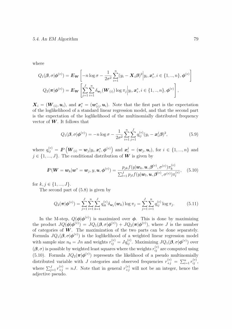
5.4. An EM Algorithm 79
where
Q1(β, σ|φ(v)) = IEW
[−n log σ − 1
2σ2
n∑i=1
(yi − X iβ)2
∣∣∣∣yi,x∗i , i ∈ 1, .., n,φ(v)
]
Q2(π|φ(v)) = IEW
J∑j=1
n∑i=1
δwj(W (i)) log πj
∣∣∣∣yi,x∗i , i ∈ 1, .., n,φ(v)
,
X i = (W (i),ui), and x∗i = (w∗
(i),ui). Note that the first part is the expectationof the loglikelihood of a standard linear regression model, and that the second partis the expectation of the loglikelihood of the multinomially distributed frequencyvector of W . It follows that
Q1(β, σ|φ(v)) = −n log σ − 1
2σ2
n∑i=1
J∑j=1
q(v)ij (yi − xj
iβ)2, (5.9)
where q(v)ij = IP
(W (i) = wj|yi,x
∗i ,φ
(v))
and xji = (wj,ui), for i ∈ 1, ..., n and
j ∈ 1, ..., J. The conditional distribution of W is given by
IP (W = wk|w∗ = wj, y, u,φ(v)) =pjkf(y|wk,u,β(v), σ(v))π
(v)k∑J
l=1 pjlf(y|wl,u,β(v), σ(v))π(v)l
, (5.10)
for k, j ∈ 1, ..., J.The second part of (5.8) is given by
Q2(π|φ(v)) =J∑
j=1
n∑i=1
J∑k=1
q(v)ik δwj
(wk) log πj =J∑
j=1
n∑i=1
q(v)ij log πj. (5.11)
In the M-step, Q(φ|φ(v)) is maximized over φ. This is done by maximizingthe product JQ(φ|φ(v)) = JQ1(β, σ|φ(v)) + JQ2(π|φ(v)), where J is the numberof categories of W . The maximization of the two parts can be done separately.Formula JQ1(β, σ|φ(v)) is the loglikelihood of a weighted linear regression model
with sample size n0 = Jn and weights r(v)ij = Jq
(v)ij . Maximizing JQ1(β, σ|φ(v)) over
(β, σ) is possible by weighted least squares where the weights r(v)ij are computed using
(5.10). Formula JQ2(π|φ(v)) represents the likelihood of a pseudo multinomially
distributed variable with J categories and observed frequencies r(v)+j =
∑ni=1 r
(v)ij ,
where∑J
j=1 r(v)+j = nJ . Note that in general r
(v)+j will not be an integer, hence the
adjective pseudo.
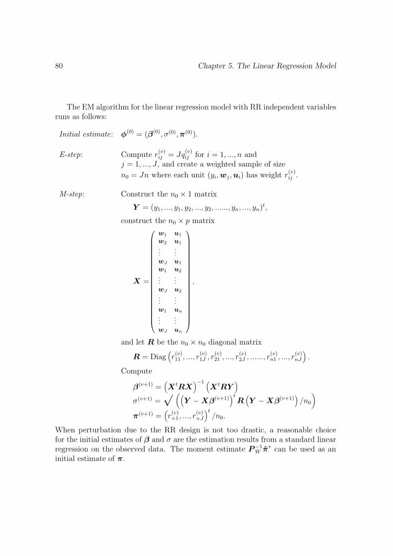
80 Chapter 5. The Linear Regression Model
The EM algorithm for the linear regression model with RR independent variablesruns as follows:
Initial estimate: φ(0) = (β(0), σ(0),π(0)).
E-step: Compute r(v)ij = Jq
(v)ij for i = 1, ..., n and
j = 1, ..., J , and create a weighted sample of size
n0 = Jn where each unit (yi,wj,ui) has weight r(v)ij .
M-step: Construct the n0 × 1 matrix
Y = (y1, ..., y1, y2, ..., y2, ......, yn, ..., yn)t,
construct the n0 × p matrix
X =
w1 u1
w2 u1
......
wJ u1
w1 u2
......
wJ u2
......
w1 un
......
wJ un
,
and let R be the n0 × n0 diagonal matrix
R = Diag(r(v)11 , ..., r
(v)1J , r
(v)21 , ..., r
(v)2J , ......, r
(v)n1 , ..., r
(v)nJ
).
Compute
β(v+1) =(X tRX
)−1 (X tRY
)σ(v+1) =
√ ((Y − Xβ(v+1)
)tR
(Y − Xβ(v+1)
)/n0
)π(v+1) =
(r(v)+1 , ..., r
(v)+J
)t/n0.
When perturbation due to the RR design is not too drastic, a reasonable choicefor the initial estimates of β and σ are the estimation results from a standard linearregression on the observed data. The moment estimate P−1
W π∗ can be used as aninitial estimate of π.
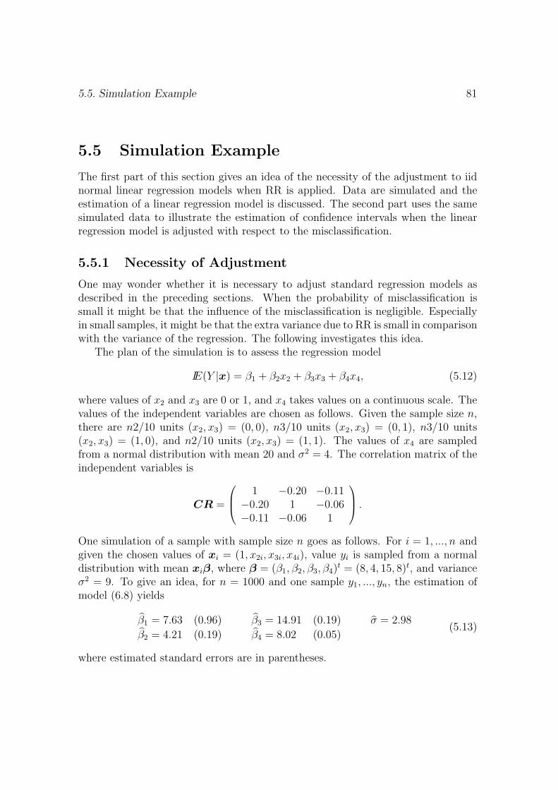
5.5. Simulation Example 81
5.5 Simulation Example
The first part of this section gives an idea of the necessity of the adjustment to iidnormal linear regression models when RR is applied. Data are simulated and theestimation of a linear regression model is discussed. The second part uses the samesimulated data to illustrate the estimation of confidence intervals when the linearregression model is adjusted with respect to the misclassification.
5.5.1 Necessity of Adjustment
One may wonder whether it is necessary to adjust standard regression models asdescribed in the preceding sections. When the probability of misclassification issmall it might be that the influence of the misclassification is negligible. Especiallyin small samples, it might be that the extra variance due to RR is small in comparisonwith the variance of the regression. The following investigates this idea.
The plan of the simulation is to assess the regression model
IE(Y |x) = β1 + β2x2 + β3x3 + β4x4, (5.12)
where values of x2 and x3 are 0 or 1, and x4 takes values on a continuous scale. Thevalues of the independent variables are chosen as follows. Given the sample size n,there are n2/10 units (x2, x3) = (0, 0), n3/10 units (x2, x3) = (0, 1), n3/10 units(x2, x3) = (1, 0), and n2/10 units (x2, x3) = (1, 1). The values of x4 are sampledfrom a normal distribution with mean 20 and σ2 = 4. The correlation matrix of theindependent variables is
CR =
1 −0.20 −0.11−0.20 1 −0.06−0.11 −0.06 1
.
One simulation of a sample with sample size n goes as follows. For i = 1, ..., n andgiven the chosen values of xi = (1, x2i, x3i, x4i), value yi is sampled from a normaldistribution with mean xiβ, where β = (β1, β2, β3, β4)
t = (8, 4, 15, 8)t, and varianceσ2 = 9. To give an idea, for n = 1000 and one sample y1, ..., yn, the estimation ofmodel (6.8) yields
β1 = 7.63 (0.96) β3 = 14.91 (0.19) σ = 2.98
β2 = 4.21 (0.19) β4 = 8.02 (0.05)(5.13)
where estimated standard errors are in parentheses.
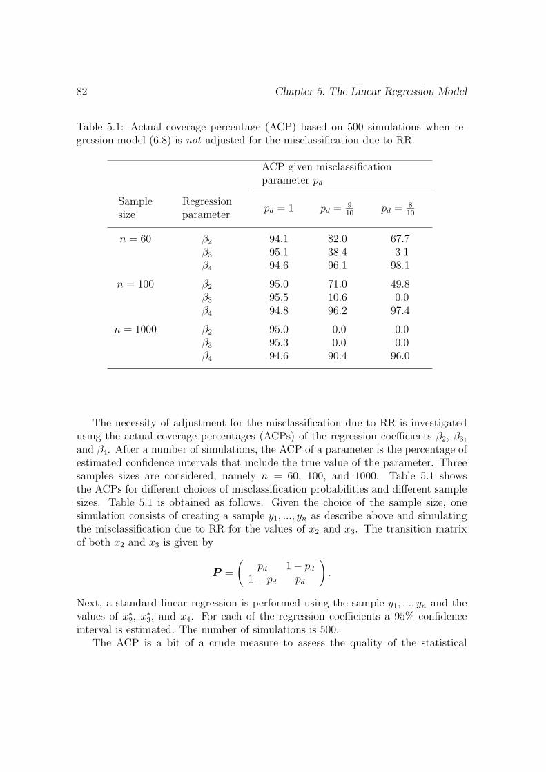
82 Chapter 5. The Linear Regression Model
Table 5.1: Actual coverage percentage (ACP) based on 500 simulations when re-gression model (6.8) is not adjusted for the misclassification due to RR.
ACP given misclassificationparameter pd
Samplesize
Regressionparameter
pd = 1 pd = 910
pd = 810
n = 60 β2 94.1 82.0 67.7β3 95.1 38.4 3.1β4 94.6 96.1 98.1
n = 100 β2 95.0 71.0 49.8β3 95.5 10.6 0.0β4 94.8 96.2 97.4
n = 1000 β2 95.0 0.0 0.0β3 95.3 0.0 0.0β4 94.6 90.4 96.0
The necessity of adjustment for the misclassification due to RR is investigatedusing the actual coverage percentages (ACPs) of the regression coefficients β2, β3,and β4. After a number of simulations, the ACP of a parameter is the percentage ofestimated confidence intervals that include the true value of the parameter. Threesamples sizes are considered, namely n = 60, 100, and 1000. Table 5.1 showsthe ACPs for different choices of misclassification probabilities and different samplesizes. Table 5.1 is obtained as follows. Given the choice of the sample size, onesimulation consists of creating a sample y1, ..., yn as describe above and simulatingthe misclassification due to RR for the values of x2 and x3. The transition matrixof both x2 and x3 is given by
P =
(pd 1 − pd
1 − pd pd
).
Next, a standard linear regression is performed using the sample y1, ..., yn and thevalues of x∗
2, x∗3, and x4. For each of the regression coefficients a 95% confidence
interval is estimated. The number of simulations is 500.The ACP is a bit of a crude measure to assess the quality of the statistical
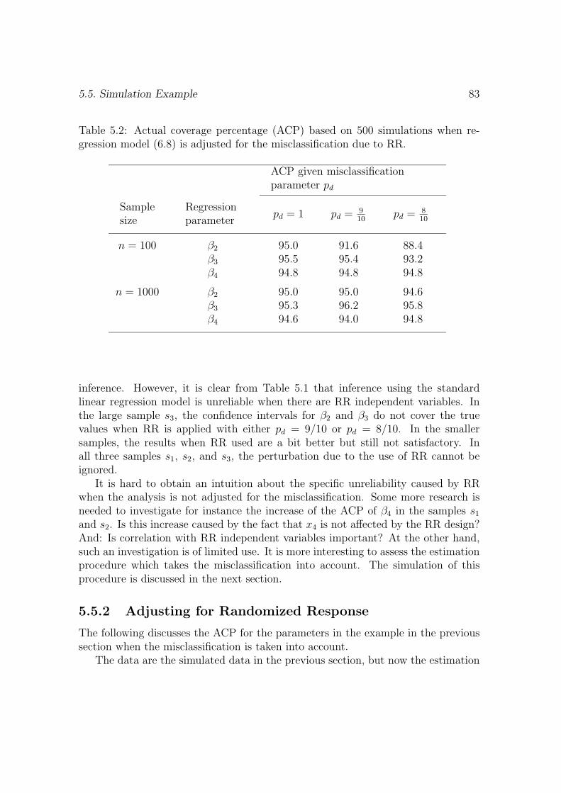
5.5. Simulation Example 83
Table 5.2: Actual coverage percentage (ACP) based on 500 simulations when re-gression model (6.8) is adjusted for the misclassification due to RR.
ACP given misclassificationparameter pd
Samplesize
Regressionparameter
pd = 1 pd = 910
pd = 810
n = 100 β2 95.0 91.6 88.4β3 95.5 95.4 93.2β4 94.8 94.8 94.8
n = 1000 β2 95.0 95.0 94.6β3 95.3 96.2 95.8β4 94.6 94.0 94.8
inference. However, it is clear from Table 5.1 that inference using the standardlinear regression model is unreliable when there are RR independent variables. Inthe large sample s3, the confidence intervals for β2 and β3 do not cover the truevalues when RR is applied with either pd = 9/10 or pd = 8/10. In the smallersamples, the results when RR used are a bit better but still not satisfactory. Inall three samples s1, s2, and s3, the perturbation due to the use of RR cannot beignored.
It is hard to obtain an intuition about the specific unreliability caused by RRwhen the analysis is not adjusted for the misclassification. Some more research isneeded to investigate for instance the increase of the ACP of β4 in the samples s1
and s2. Is this increase caused by the fact that x4 is not affected by the RR design?And: Is correlation with RR independent variables important? At the other hand,such an investigation is of limited use. It is more interesting to assess the estimationprocedure which takes the misclassification into account. The simulation of thisprocedure is discussed in the next section.
5.5.2 Adjusting for Randomized Response
The following discusses the ACP for the parameters in the example in the previoussection when the misclassification is taken into account.
The data are the simulated data in the previous section, but now the estimation
84 Chapter 5. The Linear Regression Model
of the regression model takes into account the misclassification due to RR by max-imizing (5.7). The maximization routine is a combination of two routines. First,20 EM steps are performed. Starting values are obtained by applying the standardlinear regression model to the misclassified data. Next, the result of the EM isused as the starting point of the second routine which is the standard maximiza-tion routine nlm() in the programming environment R. This second routine is aNewton-Raphson type of maximization and yields estimated standard errors.
To give an idea of the increase of the standard errors due to RR, consider thefollowing estimates for a simulated sample. The estimates were obtained by maxi-mizing (5.7).
β1 = 8.03 (1.25) β3 = 14.47 (0.26) σ = 3.09
β2 = 3.90 (0.32) β4 = 8.02 (0.06)(5.14)
These estimates concern the same sample as in (5.13) albeit that this time RR wassimulated with pd = 8/10 for the independent variables x2 and x3. Comparing (5.14)with (5.13) shows that standard errors are increased, but that they stay within areasonable range.
Table 5.2 presents results after 500 simulated samples for different sample sizesand different choices of pd. The overall impression is that the adjustment works wellwhen the sample size is large, see the results for n = 1000. For smaller samples,the simulations show that when pd decreases, the analysis becomes less reliable,see the results for n = 100. Apparently, the sample size has to be large so that theasymptotic properties of the maximum likelihood estimator dominate. Perturbationcaused by the use of RR or PRAM implies that samples sizes have to larger than instandard situations without misclassification.
5.6 Conclusion
This paper presents a method to estimate the iid normal linear regression modelwith RR independent variables. An EM algorithm is presented as an alternative toNewton-Raphson maximization of the loglikelihood. In general, an EM algorithm isconsidered a stable but a somewhat slow maximization routine and when a Newton-Raphson type of algorithm is possible, it is preferred since it is faster and the esti-mation of standard errors is almost automatic. However, the present loglikelihoodcan be quite complex numerically. Especially in the case of PRAM, there might bea large number of perturbed independent variables some of which may have a large
5.6. Conclusion 85
number of categories. Consider a model that includes the variables Gender (2 cate-gories), Ethnic Background (4 categories), and Region (20 categories). Assume thatPRAM is applied. Besides the regression parameters, there are 2× 4× 20− 1 = 159nuisance parameters in the maximization of (5.7).
Using ready-made maximization routines to maximize the loglikelihood is anoption, but these routines will also be sensitive to ill-chosen starting values. Fur-thermore, ready-made routines are blind with respect to the structure of the maxi-mization problem. The EM presented in this paper explicitly uses the structure ofthe linear regression model. Since the maximization in the M-step is of closed form,the EM algorithm is actually quite fast. It is possible to use EM and extend themaximization with a general method that yields estimated standard errors in EMmaximization, see, e.g., the discussion of the supplemented EM in Little and Rubin(2002, Section 9.2).
The simulations in Section 5.5 show that the perturbation caused by using RRor PRAM cannot be ignored. Furthermore, the simulations demonstrate that themethod presented in this paper is feasible and that adjustment for the perturbationis possible. However, sample sizes have to be larger than in the standard situationwithout perturbation. Protecting privacy is not for free.
Estimation of the parameters in the linear regression model is only the first step infitting a linear regression model to data. Future research should address possibilitiesto check some of the assumptions of the model. Can outliers for instance be detectedwhen some of the independent variables are subject to misclassification?
Although this paper only discusses the iid normal linear regression model, itmight be interesting to investigate the approach for more sophisticated regressionmodels. The reclassification model will stay the same, but it might be that a straight-forward EM is not possible anymore.

86

Chapter 6
Variants of PRAM and Measuresfor Disclosure Risk
6.1 Introduction
The post randomization method (PRAM) is discussed in Gouweleeuw, Kooiman,Willenborg, and De Wolf (1998) as a method for statistical disclosure control (SDC).When survey data are released by statistical agencies, SDC protects the identitiesof respondents. SDC tries to prevent that a user of released data can link data of arespondent in the survey to a specific person in the population. See Willenborg andDe Waal (2001) for an introduction into SDC and SDC methods other than PRAM.
There is a close link between PRAM and randomized response, a method to asksensitive questions in a survey, see Warner (1965) and Rosenberg (1979). Van denHout and Van der Heijden (2002) sum up some differences and similarities betweenrandomized response and PRAM.
When SDC is used, there will always be a loss of information. This is inevitablesince SDC tries to determine the information in the data that can lead to the dis-closure of an identity of a respondent, and eliminates this information before dataare released. It is not difficult to prevent disclosure, but it is difficult to preventdisclosure and release data that is still useful for statistical analysis. Applying SDCmeans searching for a balance between disclosure risk and information loss.
The idea of PRAM is to misclassify some of the categorical variables in the sur-vey using fixed misclassification probabilities and to release the partly misclassifieddata together with those probabilities. Say variable X, with categories 1, ..., J,
1This chapter is joint work with Elsayed Elamir, University of Southampton, United Kingdom.
87
88 Chapter 6. Variants of PRAM and Measures for Disclosure Risk
is misclassified into variable X∗. The survey containing X∗ but not X is releasedtogether with conditional probabilities IP (X∗ = k|X = j), for k, j ∈ 1, ..., J. Inthis way, PRAM introduces uncertainty in the data: The user of the released datacannot be sure that the information is original or perturbed due to PRAM and itbecomes harder to establish a correct link between a respondent in the survey anda specific person in the population. Since the user has the misclassification proba-bilities, he can adjust his analysis by taking into account the perturbation due toPRAM.
This paper discusses two ideas to make PRAM more efficient with respect to thebalance between disclosure risk and information loss. First, the paper discusses theuse of calibration probabilities
IP (true category is j|category i is released). (6.1)
in the analysis of released data and compares this with using misclassification prob-abilities
IP (category i is released|true category is j). (6.2)
The idea of using calibration probabilities is discussed by De Wolf, Gouweleeuw,Kooiman, and Willenborg (1997), who refer to the discussion of calibration proba-bilities in misclassification literature, see, e.g., Kuha and Skinner (1997). We willelaborate the discussion and show that the advantage of calibration probabilitiesis limited to the univariate case. Secondly, the paper shows that information losscan be reduced by providing misclassification proportions along with the releaseddata. These proportions inform about the actual change in the survey data due tothe application of PRAM. (Probabilities (6.1) and (6.2) inform about the expectedchange.) In addition, the paper discusses two measures for disclosure risk whenPRAM is applied. The first is an extension of the measure introduced by Skinnerand Elliot (2002). The second measure links up with the SDC practice at StatisticNetherlands. Simulation results are given to illustrate the theory.
The outline of the paper is as follows. Section 6.2 provides the framework andthe notation. Section 6.3 describes frequency estimation for PRAM data. Section6.4 discusses the use of calibration probabilities. In Section 6.5, we introduce the useof misclassification proportions. Section 6.6 discusses measures for disclosure risk,whereas information loss is briefly considered in Section 6.7. Section 6.8 presentssome simulations, and Section 6.9 concludes.

6.2. Framework and Notation 89
6.2 Framework and Notation
In survey data, we distinguish between identifying variables and non-identifyingvariables. Identifying variables are variables that can be used to re-identify individ-uals represented in the data. These variables are assumed to be categorical, e.g.,Gender, Race, Place of Residence. We assume that the sensitive information of re-spondents is contained in the non-identifying variables, see Bethlehem, Keller, andPannekoek (1990), and that we want to protect this information by applying PRAMto (a subset of) the identifying variables.
The notation in this paper is the same as in Skinner and Elliot (2002). Unitsare selected from a finite population U and each selected unit has one record in themicrodata sample s ⊂ U . Let n denote the number of units in s. Let the categoricalvariable formed by cross-classifying (a subset of) the identifying variables be denotedX with values in 1, ..., J. Let Xi denote the value of X for unit i ∈ U . Thepopulation frequencies are denoted
Fj =∑i∈U
I(Xi = j), j ∈ 1, ..., J,
where I(·) is the indicator function: I(A) = 1 if A is true and I(A) = 0 otherwise.The sample frequencies are denoted
fj =∑i∈s
I(Xi = j), j ∈ 1, ..., J.
In the framework of PRAM, we call the sample that is released by the statisticalagency the released microdata sample s∗. Note that unit i ∈ s∗ if and only if i ∈ s.Let X∗ denote the released version of X in s∗. By misclassification of unit i wemean Xi = X∗
i . The released sample frequencies are denoted
f ∗k =
∑i∈s∗
I(X∗i = k), k ∈ 1, ..., J.
Let P X denote the J × J transition matrix that contains the conditional misclas-sification probabilities pkj = IP (X∗ = k|X = j), for k, j ∈ 1, ..., J. Note thatthe columns of P X sum up to one. The distribution of X∗ conditional on s is theJ-component finite mixture given by
IP (X∗i = k|i ∈ s) =
J∑j=1
IP (X∗i = k|Xi = j)IP (Xi = j|i ∈ s), k ∈ 1, ..., J,
90 Chapter 6. Variants of PRAM and Measures for Disclosure Risk
where the component distributions are given by P X and the component weights aregiven by the conditional distribution of X. The conditional distribution of X insample s is given by
IP (Xi = j|i ∈ s) =1
nfj, j ∈ 1, ..., J.
6.3 Frequency Estimation for PRAM Data
When PRAM is applied and some of the identifying variables are misclassified,standard statistical models do not apply to the released data since these models donot take into account the perturbation. This section shows how the misclassificationcan be taken into account in frequency estimation.
We have IE[F ∗|f ] = P Xf , where f = (f1, ..., fJ)t and F ∗ = (F ∗1 , ..., F ∗
J )t is thestochastic vector of the released sample frequencies. An unbiased moment estimatorof f is given by
f = P−1X f ∗, (6.3)
see Kooiman, Willenborg, and Gouweleeuw (1997). In practice, assuming that P X isnon-singular does not impose much restriction on the choice of the misclassificationprobabilities. Matrix P−1
X exists when the diagonal of P X dominates, i.e., pii > 1/2for i ∈ 1, ..., J. An additional assumption in (6.3) is that the dimensions of f andf ∗ are the same.
PRAM is applied to each variable independently and a transition matrix is re-leased per variable. When the user of the released sample assesses a compoundedvariable, he can construct its transition matrix using the transition matrices ofthe individual variables. For instance, consider identifying variables X1, with cat-egories 1, .., J1 and X2, with categories 1, .., J2, and the cross-classificationX = (X1, X2), i.e., the Cartesian product of X1 and X2. Since PRAM is appliedindependently, we have
IP(X∗ = (k1, k2)|X = (j1, j2)
)= IP (X∗
1 = k1|X1 = j1)
× IP (X∗2 = k2|X1 = j2), (6.4)
for k1, j1 ∈ 1, .., J1 and k2, j2 ∈ 1, .., J2. In matrix notation, we have P X =P X1 ⊗P X2 , where ⊗ is the Kronecker product. Note that when one of two variablesis not perturbed by PRAM, the transition matrix of that variable is the identitymatrix.
6.4. Calibration Probabilities 91
The variance of (6.3) equals
V [f |f ] = P−1X V [F ∗|f ](P−1
X )t = P−1X
( J∑j=1
fjV j
)(P−1
X )t (6.5)
where V j is the J × J covariance matrix of two released values given the originalvalue j, i.e.,
V j(k1, k2) =
pk2j(1 − pk2j) if k1 = k2
−pk1jpk2j if k1 = k2
for k1, k2 ∈ 1, ..., J,
see Kooiman et al. (1997). The variance can be estimated by substituting fj for fj
in (6.5), for j ∈ 1, .., J.The variance given by (6.5) is the extra variance due to PRAM and does not
take into account the sampling distribution. The formulas for the latter are givenin Chaudhuri and Mukerjee (1988) for multinomial sampling and compared to (6.5)in Van den Hout and Van der Heijden (2002), see also Appendix 6.B.
6.4 Calibration Probabilities
Literature concerning misclassification shows that calibration probabilities (6.1) aremore efficient in the analysis of misclassified data than misclassification probabil-ities (6.2), see the review paper by Kuha and Skinner (1997). Often, calibrationprobabilities have to be estimated. However, when PRAM is applied, the statisti-cal agency can compute the calibration probabilities using the sample frequencies.The idea of using calibration probabilities for PRAM is mentioned in De Wolf et al.(1997). The following elaborates this idea and makes a comparison with PRAM asexplained in the previous section.
The J×J matrix with calibration probabilities of univariate variable X is denotedby
←−P X and has entries ←−p jk defined by
IP (Xi = j|X∗i = k, i ∈ s) =
pkjfj∑Jj0=1 pkj0fj0
, j, k ∈ 1, ..., J, (6.6)
where pkj are the entries of P X . Matrix←−P X is again a transition matrix; each
column sums up to one. We have
f =←−P XIE[F ∗|f ], (6.7)
92 Chapter 6. Variants of PRAM and Measures for Disclosure Risk
see Appendix 6.A. An unbiased moment estimator of f is therefore given by
f =←−P Xf ∗. (6.8)
In general,←−P X = P−1
X , see Appendix 6.A. The variance of (6.8) is given by (6.5)
where P−1X is replaced by
←−P X and fj is estimated by fj, for j ∈ 1, ..., J.
In the remainder of this section we compare estimators (6.3) and (6.8). Thefirst difference is that (6.3) might yield an estimate where some of the entries arenegative, whereas (6.8) will never yield negative estimates, see, e.g., De Wolf et al.(1997).
Secondly, estimator (6.8) is more efficient than (6.3) in the univariate case. Thisis already discussed in Kuha and Skinner (1997). Consider the case where X hastwo categories. Say we want to know π = IP (X = 1). Let π be the estimate using
P X and π the estimate using←−P X . The efficiency of π relative to π is given by
eff(π, π) =V [p ]
V [p ]= (p11 + p22 − 1)2(←−p 22 −←−p 21)
2 < 1. (6.9)
So π is always more efficient than π. An important difference with the generalsituation of misclassification is that in the situation of PRAM, matrices P X and←−P X are given and do not have to be estimated. Comparison (6.9) is therefore asimple form of the comparison in Kuha and Skinner (1997, Section 28.5.1.3.).
The third comparison is between the maximum likelihood properties of (6.3) and(6.8). Assume that the frequency vector f of X1, ...Xn is multinomially distributedwith parameters n and π = (π1, .., πJ)t. In the framework of misclassification,Hochberg (1977) proves that estimator (6.8) yields an MLE. When (6.3) yieldsan estimate in the interior of the parameter space, the estimate is also an MLE.See Appendix 6.B for the maximum likelihood properties of (6.8) and (6.3). Thelikelihood function corresponding to (6.8) is different from the likelihood functioncorresponding to (6.3), since the information used is different. This explains whyboth can be an MLE despite being different estimators of f .
The fourth comparison is with respect to transition matrices of Cartesian prod-ucts and is less favorable for (6.8). It has already been noted that P X1 ⊗ P X2
is the matrix with misclassification probabilities for the Cartesian product X =(X1, X2), see (6.4). Analogously, given
←−P X1 and
←−P X2 the user can construct ma-
trix←−P X1 ⊗ ←−
P X2 . However, this matrix does not necessarily contain calibrationprobabilities for X. Note that
6.5. Misclassification Proportions 93
IP(Xi = (j1, j2)|X∗
i = (k1, k2), i ∈ s)
=pk1j1pk2j2IP
(Xi = (j1, j2)|i ∈ s
)∑J1
v
∑J2w pk1vpk2wIP
(X1 = (v, w)|i ∈ s
) . (6.10)
It follows that←−P X =
←−P X1 ⊗ ←−
P X2 when X1 and X2 are independent. In general,this independence is not guaranteed and since the user of the released data does nothave the frequencies of X, he cannot construct
←−P X .
The fifth and last comparison is with respect to the creation of subgroups. Con-sider the situation where a user of the released data creates a subgroup by usinga grouping variable that is not part of X. When the number of categories in thesubgroup is smaller than J , estimate (6.8) is not well-defined. When the number ofcategories is equal to J , estimate (6.8) is biased due to the fact that (6.7) does not
hold. Note with respect to (6.7) that the frequencies that are used to construct←−P X
are the frequencies in the whole sample which will differ from the frequencies in thesubgroup, see also Appendix 6.A. Estimator (6.3) is still valid for the subgroup.
Since calibration probabilities contain information about the distribution of thesample s, they perform better than misclassification probabilities regarding the uni-variate case. However, in a multivariate setting this advantage may disappear.Section 6.8 presents some simulation results.
6.5 Misclassification Proportions
Matrices P X and←−P X inform about the expected change due to PRAM. As an alter-
native, we can create transition matrices that inform about the actual change duean application of PRAM. These matrices contain proportions and will be denotedP
X and←−P
X . Matrix P
X contains misclassification proportions and←−P
X contains
calibration proportions. This section shows how P X and
←−P
X are computed and
discusses properties of these matrices.We start with an example. Say that X has categories 1,2. Assume that
applying PRAM yields the cross-classification in Table 6.1. From this table it followsthat the proportion of records with X = 1 that have X∗ = 1 in the released sampleis 300/400=3/4 and that the proportion of records with X∗ = 1 that have X = 1 inthe original sample is 300/500=3/5. Analogously we get the other entries of
P X =
(3/4 1/31/4 2/3
)and
←−P
X =
(3/5 1/52/5 4/5
).
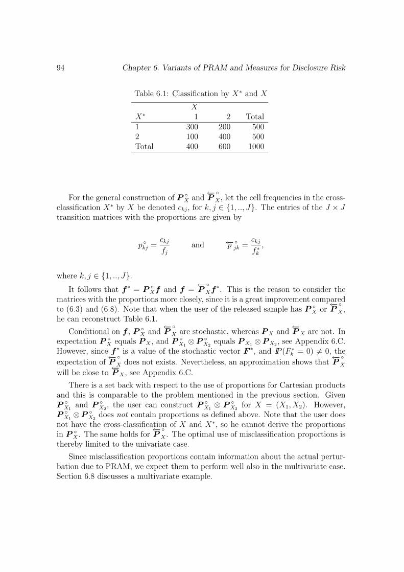
94 Chapter 6. Variants of PRAM and Measures for Disclosure Risk
Table 6.1: Classification by X∗ and X
XX∗ 1 2 Total1 300 200 5002 100 400 500Total 400 600 1000
For the general construction of P X and
←−P
X , let the cell frequencies in the cross-
classification X∗ by X be denoted ckj, for k, j ∈ 1, .., J. The entries of the J × Jtransition matrices with the proportions are given by
p kj =
ckj
fj
and ←−p jk =
ckj
f ∗k
,
where k, j ∈ 1, .., J.It follows that f ∗ = P
Xf and f =←−P
Xf ∗. This is the reason to consider the
matrices with the proportions more closely, since it is a great improvement comparedto (6.3) and (6.8). Note that when the user of the released sample has P
X or←−P
X ,
he can reconstruct Table 6.1.
Conditional on f , P X and
←−P
X are stochastic, whereas P X and
←−P X are not. In
expectation P X equals P X , and P
X1⊗P
X2equals P X1 ⊗P X2 , see Appendix 6.C.
However, since f ∗ is a value of the stochastic vector F ∗, and IP (F ∗k = 0) = 0, the
expectation of←−P
X does not exists. Nevertheless, an approximation shows that
←−P
X
will be close to←−P X , see Appendix 6.C.
There is a set back with respect to the use of proportions for Cartesian productsand this is comparable to the problem mentioned in the previous section. GivenP
X1and P
X2, the user can construct P
X1⊗ P
X2for X = (X1, X2). However,
P X1
⊗P X2
does not contain proportions as defined above. Note that the user doesnot have the cross-classification of X and X∗, so he cannot derive the proportionsin P
X . The same holds for←−P
X . The optimal use of misclassification proportions is
thereby limited to the univariate case.
Since misclassification proportions contain information about the actual pertur-bation due to PRAM, we expect them to perform well also in the multivariate case.Section 6.8 discusses a multivariate example.
6.6. Disclosure Risk 95
6.6 Disclosure Risk
There are several ways to measure disclosure risk (Skinner and Elliot 2002; Domingo-Ferrer and Torra 2001). This section discusses two measures for disclosure risk withrespect to PRAM. Section 6.6.1 discusses an extension of the general measure ofdisclosure risk introduced by Skinner and Elliot (2002). Section 6.6.2 introduces ameasure that links up with the way disclosure risk is assessed at Statistics Nether-lands.
6.6.1 The Measure Theta
The following describes how the general measure for disclosure risk introduced inSkinner and Elliot (2002) can be extended to the situation where PRAM is appliedbefore data are released by the statistical agency. When a disclosure control methodsuch as PRAM has been applied, a measure for disclosure risk is needed to quantifythe protection that is offered by the control method. Scenarios that may lead to adisclosure of the identity of a respondent are about persons that aim at disclosureand that may have data that overlap the released data. A common scenario is thata person has a sample from another source and tries to identify respondents in thereleased sample by matching records. Using an extension of the measure in Skinnerand Elliot (2002) we can investigate how applying PRAM reduces the disclosurerisk.
Under simple random sampling, Skinner and Elliot (2002) introduced the mea-sure of disclosure risk θ = IP (correct match|unique match) as
θ =
∑Jj=1 I(fj = 1)∑J
j=1 Fj I(fj = 1).
The measure θ is the proportion of correct matches among those population unitswhich match a sample unique. The measure is sample dependent and a distribution-free prediction is given by
θ =πn1
πn1 + 2(1 − π)n2
,
where π is the sampling fraction, n1 =∑J
j=1 I(fj = 1) is the number of uniques and
n2 =∑J
j=1 I(fj = 2) is the number of twins in the sample (Skinner and Elliot 2002).Elamir and Skinner (2003) extended θ for the situation where misclassification oc-curs. The extension is given by
θmm =
∑i∈s I(fXi
= 1, X∗i = Xi)∑J
j=1 Fj I(fj = 1)
96 Chapter 6. Variants of PRAM and Measures for Disclosure Risk
and its distribution-free prediction is given by
θmm =π∑J
j=1 I(fj = 1)pjj
πn1 + 2 (1 − π) n2
,
where pjj is the diagonal entry (j, j) of the transition matrix P X which describesthe misclassification.
Section 6.8 presents some simulation results with respect to the measure θ beforeapplying PRAM, and θmm after applying PRAM.
6.6.2 Spontaneous Recognition
Statistics Netherlands releases data in several ways one of which is releasing detailedsurvey data under contract. Data are released under contract to bona fide researchinstitutes that sign an agreement in which they promise not to look for disclosureexplicitly, e.g, by matching the data to other data files. In this situation, SDCconcerns the protection against what is called spontaneous recognition. This sectionintroduces a measure for disclosure risk for PRAM data that is specific to the controlfor spontaneous recognition.
Controlling for spontaneous recognition means that one should prevent that cer-tain records attract attention. A record may attract attention when a low dimen-sional combination of its values has a low frequency. Also, without cross-classifying,a record may attract attention when one of its values is recognized as being veryrare in the population. Combinations of values with low frequencies in the sampleare called unsafe combinations.
Statistics Netherlands uses the rule of thumb that a recognition of a combinationof values of more than three variables is not spontaneous anymore. For this reason,only combinations of three variables are assessed with respect to disclosure controlfor spontaneous recognition.
Note that applying PRAM causes two kinds of modifications in the sample thatmake disclosure more difficult. First, it is possible that unsafe combinations in thesample change into apparently safe ones in the released sample, and, secondly, it ispossible that safe combinations in the sample change into apparently unsafe ones.Since misclassification probabilities are not that large (in order to keep analysis ofthe released sample possible) and the frequency of unsafe combinations is typicallylow, the effect of the first modification is negligible in expectation. The secondmodification is more likely to protect an unsafe combination j when there are alot of combinations k, k = j, which are misclassified into j. This is the reason to
6.7. Information Loss 97
focus, for a given record i with the unsafe combination of scores j, on the calibrationprobability
µ = IP (Xi = j|X∗i = j, i ∈ s).
When there are hardly any k, k = j, misclassified into j, this probability will belarge, and, as a consequence, the released record is unsafe. Note that combinationswith frequency equal to zero are never unsafe.
Measure µ is a simplification since it ignores possible correlation between X andother variables in the sample. Note that X will be a Cartesian product and thatthe statistical agency can compute the calibration probability µ using (6.6) sincethe agency has the frequencies of X.
6.7 Information Loss
Since we stressed in the introduction that SDC means searching for a balance be-tween disclosure risk and information loss, this section indicates ways to investigateinformation loss due to PRAM.
First, the transition matrix P X gives an idea of the loss of information. Themore this matrix resembles the identity matrix, the less information gets lost. Ingeneral, this requires a definition of a distance between two matrices. However, wecan apply PRAM using matrices that are parameterized by one parameter, denotedpd. The idea is as follows. Each time PRAM is applied, the diagonal probabilitiesin a transition matrix are fixed and equal to pd. In the columns, the probabilitymass 1− pd is equally divided over the entries that are not diagonal entries. In thissituation 1 − pd is a measure for the deviation from the identity matrix.
Although transition matrices give an idea of the information loss, it is hard tohave an intuition about how a certain deviation from the identity matrix affectsanalysis of the released data. A second way to investigate information loss is thecomparison of extra variances due to PRAM with respect to frequency estimation.The idea here is that when this extra variance is already substantial, more complexanalyses of the released sample is probably not possible. The variance with respectto frequency estimation can be estimated using (6.5).
The next section will assess information loss due to PRAM using these twoapproaches.
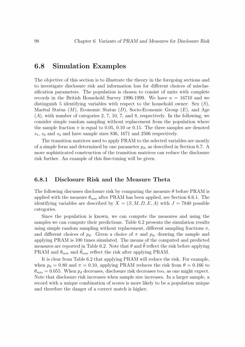
98 Chapter 6. Variants of PRAM and Measures for Disclosure Risk
6.8 Simulation Examples
The objective of this section is to illustrate the theory in the foregoing sections andto investigate disclosure risk and information loss for different choices of misclas-sification parameters. The population is chosen to consist of units with completerecords in the British Household Survey 1996-1999. We have n = 16710 and wedistinguish 5 identifying variables with respect to the household owner: Sex (S),Marital Status (M), Economic Status (D), Socio-Economic Group (E), and Age(A), with number of categories 2, 7, 10, 7, and 8, respectively. In the following, weconsider simple random sampling without replacement from the population wherethe sample fraction π is equal to 0.05, 0.10 or 0.15. The three samples are denoteds1, s2 and s3 and have sample sizes 836, 1671 and 2506 respectively.
The transition matrices used to apply PRAM to the selected variables are mostlyof a simple form and determined by one parameter pd, as described in Section 6.7. Amore sophisticated construction of the transition matrices can reduce the disclosurerisk further. An example of this fine-tuning will be given.
6.8.1 Disclosure Risk and the Measure Theta
The following discusses disclosure risk by comparing the measure θ before PRAM isapplied with the measure θmm after PRAM has been applied, see Section 6.6.1. Theidentifying variables are described by X = (S,M,D,E,A) with J = 7840 possiblecategories.
Since the population is known, we can compute the measures and using thesamples we can compute their predictions. Table 6.2 presents the simulation resultsusing simple random sampling without replacement, different sampling fractions π,and different choices of pd. Given a choice of π and pd, drawing the sample andapplying PRAM is 100 times simulated. The means of the computed and predictedmeasures are reported in Table 6.2. Note that θ and θ reflect the risk before applyingPRAM and θmm and θmm reflect the risk after applying PRAM.
It is clear from Table 6.2 that applying PRAM will reduce the risk. For example,when pd = 0.80 and π = 0.10, applying PRAM reduces the risk from θ = 0.166 toθmm = 0.055. When pd decreases, disclosure risk decreases too, as one might expect.Note that disclosure risk increases when sample size increases. In a larger sample, arecord with a unique combination of scores is more likely to be a population uniqueand therefore the danger of a correct match is higher.
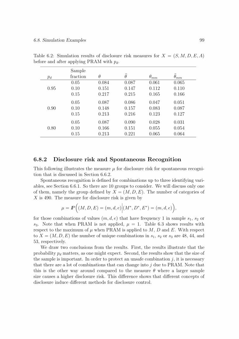
6.8. Simulation Examples 99
Table 6.2: Simulation results of disclosure risk measures for X = (S,M,D,E,A)before and after applying PRAM with pd.
pd
Samplefraction θ θ θmm θmm
0.05 0.084 0.087 0.061 0.0650.95 0.10 0.151 0.147 0.112 0.110
0.15 0.217 0.215 0.165 0.166
0.05 0.087 0.086 0.047 0.0510.90 0.10 0.148 0.157 0.083 0.087
0.15 0.213 0.216 0.123 0.127
0.05 0.087 0.090 0.028 0.0310.80 0.10 0.166 0.151 0.055 0.054
0.15 0.213 0.221 0.065 0.064
6.8.2 Disclosure risk and Spontaneous Recognition
This following illustrates the measure µ for disclosure risk for spontaneous recogni-tion that is discussed in Section 6.6.2.
Spontaneous recognition is defined for combinations up to three identifying vari-ables, see Section 6.6.1. So there are 10 groups to consider. We will discuss only oneof them, namely the group defined by X = (M,D,E). The number of categories ofX is 490. The measure for disclosure risk is given by
µ = IP((M,D,E) = (m, d, e)
∣∣∣∣(M∗, D∗, E∗) = (m, d, e)),
for those combinations of values (m, d, e) that have frequency 1 in sample s1, s2 ors3. Note that when PRAM is not applied, µ = 1. Table 6.3 shows results withrespect to the maximum of µ when PRAM is applied to M , D and E. With respectto X = (M,D,E) the number of unique combinations in s1, s2 or s3 are 48, 44, and53, respectively.
We draw two conclusions from the results. First, the results illustrate that theprobability pd matters, as one might expect. Second, the results show that the size ofthe sample is important. In order to protect an unsafe combination j, it is necessarythat there are a lot of combinations that can change into j due to PRAM. Note thatthis is the other way around compared to the measure θ where a larger samplesize causes a higher disclosure risk. This difference shows that different concepts ofdisclosure induce different methods for disclosure control.
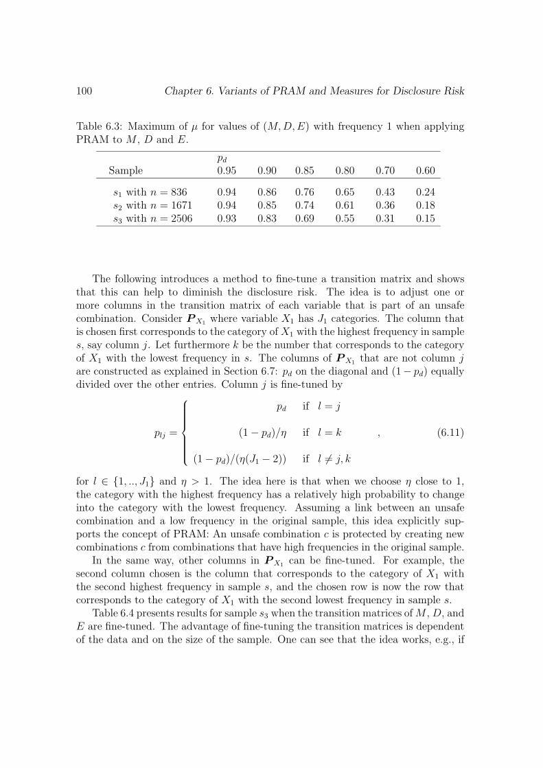
100 Chapter 6. Variants of PRAM and Measures for Disclosure Risk
Table 6.3: Maximum of µ for values of (M,D,E) with frequency 1 when applyingPRAM to M , D and E.
pd
Sample 0.95 0.90 0.85 0.80 0.70 0.60
s1 with n = 836 0.94 0.86 0.76 0.65 0.43 0.24s2 with n = 1671 0.94 0.85 0.74 0.61 0.36 0.18s3 with n = 2506 0.93 0.83 0.69 0.55 0.31 0.15
The following introduces a method to fine-tune a transition matrix and showsthat this can help to diminish the disclosure risk. The idea is to adjust one ormore columns in the transition matrix of each variable that is part of an unsafecombination. Consider P X1 where variable X1 has J1 categories. The column thatis chosen first corresponds to the category of X1 with the highest frequency in samples, say column j. Let furthermore k be the number that corresponds to the categoryof X1 with the lowest frequency in s. The columns of P X1 that are not column jare constructed as explained in Section 6.7: pd on the diagonal and (1− pd) equallydivided over the other entries. Column j is fine-tuned by
plj =
pd if l = j
(1 − pd)/η if l = k ,
(1 − pd)/(η(J1 − 2)) if l = j, k
(6.11)
for l ∈ 1, .., J1 and η > 1. The idea here is that when we choose η close to 1,the category with the highest frequency has a relatively high probability to changeinto the category with the lowest frequency. Assuming a link between an unsafecombination and a low frequency in the original sample, this idea explicitly sup-ports the concept of PRAM: An unsafe combination c is protected by creating newcombinations c from combinations that have high frequencies in the original sample.
In the same way, other columns in P X1 can be fine-tuned. For example, thesecond column chosen is the column that corresponds to the category of X1 withthe second highest frequency in sample s, and the chosen row is now the row thatcorresponds to the category of X1 with the second lowest frequency in sample s.
Table 6.4 presents results for sample s3 when the transition matrices of M , D, andE are fine-tuned. The advantage of fine-tuning the transition matrices is dependentof the data and on the size of the sample. One can see that the idea works, e.g., if
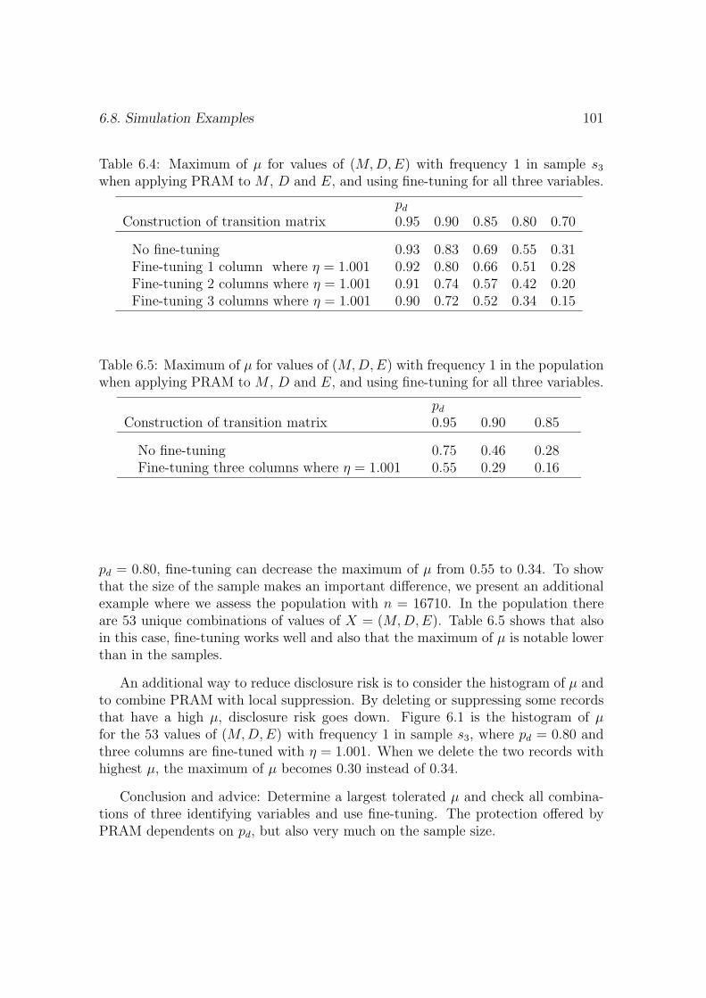
6.8. Simulation Examples 101
Table 6.4: Maximum of µ for values of (M,D,E) with frequency 1 in sample s3
when applying PRAM to M , D and E, and using fine-tuning for all three variables.
pd
Construction of transition matrix 0.95 0.90 0.85 0.80 0.70
No fine-tuning 0.93 0.83 0.69 0.55 0.31Fine-tuning 1 column where η = 1.001 0.92 0.80 0.66 0.51 0.28Fine-tuning 2 columns where η = 1.001 0.91 0.74 0.57 0.42 0.20Fine-tuning 3 columns where η = 1.001 0.90 0.72 0.52 0.34 0.15
Table 6.5: Maximum of µ for values of (M,D,E) with frequency 1 in the populationwhen applying PRAM to M , D and E, and using fine-tuning for all three variables.
pd
Construction of transition matrix 0.95 0.90 0.85
No fine-tuning 0.75 0.46 0.28Fine-tuning three columns where η = 1.001 0.55 0.29 0.16
pd = 0.80, fine-tuning can decrease the maximum of µ from 0.55 to 0.34. To showthat the size of the sample makes an important difference, we present an additionalexample where we assess the population with n = 16710. In the population thereare 53 unique combinations of values of X = (M,D,E). Table 6.5 shows that alsoin this case, fine-tuning works well and also that the maximum of µ is notable lowerthan in the samples.
An additional way to reduce disclosure risk is to consider the histogram of µ andto combine PRAM with local suppression. By deleting or suppressing some recordsthat have a high µ, disclosure risk goes down. Figure 6.1 is the histogram of µfor the 53 values of (M,D,E) with frequency 1 in sample s3, where pd = 0.80 andthree columns are fine-tuned with η = 1.001. When we delete the two records withhighest µ, the maximum of µ becomes 0.30 instead of 0.34.
Conclusion and advice: Determine a largest tolerated µ and check all combina-tions of three identifying variables and use fine-tuning. The protection offered byPRAM dependents on pd, but also very much on the sample size.
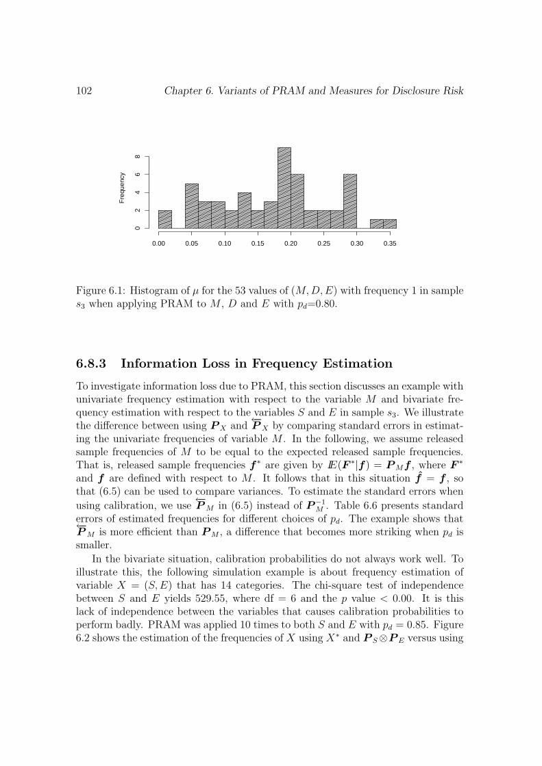
102 Chapter 6. Variants of PRAM and Measures for Disclosure Risk
Fre
quen
cy
0.00 0.05 0.10 0.15 0.20 0.25 0.30 0.35
02
46
8
Figure 6.1: Histogram of µ for the 53 values of (M,D,E) with frequency 1 in samples3 when applying PRAM to M , D and E with pd=0.80.
6.8.3 Information Loss in Frequency Estimation
To investigate information loss due to PRAM, this section discusses an example withunivariate frequency estimation with respect to the variable M and bivariate fre-quency estimation with respect to the variables S and E in sample s3. We illustratethe difference between using P X and
←−P X by comparing standard errors in estimat-
ing the univariate frequencies of variable M . In the following, we assume releasedsample frequencies of M to be equal to the expected released sample frequencies.That is, released sample frequencies f ∗ are given by IE(F ∗|f) = P Mf , where F ∗
and f are defined with respect to M . It follows that in this situation f = f , sothat (6.5) can be used to compare variances. To estimate the standard errors when
using calibration, we use←−P M in (6.5) instead of P−1
M . Table 6.6 presents standarderrors of estimated frequencies for different choices of pd. The example shows that←−P M is more efficient than P M , a difference that becomes more striking when pd issmaller.
In the bivariate situation, calibration probabilities do not always work well. Toillustrate this, the following simulation example is about frequency estimation ofvariable X = (S,E) that has 14 categories. The chi-square test of independencebetween S and E yields 529.55, where df = 6 and the p value < 0.00. It is thislack of independence between the variables that causes calibration probabilities toperform badly. PRAM was applied 10 times to both S and E with pd = 0.85. Figure6.2 shows the estimation of the frequencies of X using X∗ and P S⊗P E versus using
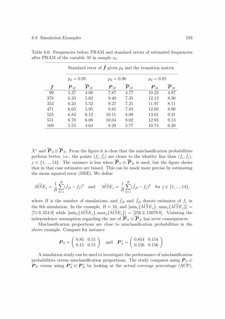
6.8. Simulation Examples 103
Table 6.6: Frequencies before PRAM and standard errors of estimated frequenciesafter PRAM of the variable M in sample s3.
Standard error of f given pd and the transition matrix
pd = 0.95 pd = 0.90 pd = 0.85
f P M←−P M P M
←−P M P M
←−P M
99 5.27 4.08 7.87 4.77 10.23 4.87378 6.33 5.62 9.40 7.35 12.13 8.30353 6.24 5.52 9.27 7.21 11.97 8.11471 6.65 5.95 9.85 7.83 12.69 8.90525 6.83 6.12 10.11 8.08 13.01 9.21551 6.78 6.08 10.04 8.02 12.93 9.13169 5.55 4.64 8.28 5.77 10.74 6.20
X∗ and←−P S ⊗←−
P E. From the figure it is clear that the misclassification probabilitiesperform better, i.e., the points (fj, fj) are closer to the identity line than (fj, fj),
j ∈ 1, ..., 14. The variance is less when←−P S ⊗ ←−
P E is used, but the figure showsthat in that case estimates are biased. This can be made more precise by estimatingthe mean squared error (MSE). We define
MSEj =1
B
B∑b=1
(fjb − fj)2 and MSEj =
1
B
B∑b=1
(fjb − fj)2 for j ∈ 1, ..., 14,
where B is the number of simulations, and fjb and fjb denote estimates of fj in
the bth simulation. In the example, B = 10, and [minjMSEj, maxjMSEj] =
[71.9, 354.9] while [minjMSEj, maxjMSEj] = [256.2, 13079.8]. Violating the
independence assumption regarding the use of←−P S ⊗←−
P E has sever consequences.Misclassification proportions are close to misclassification probabilities in the
above example. Compare for instance
P S =
(0.85 0.150.15 0.15
)and P
S =
(0.854 0.1540.156 0.156
).
A simulation study can be used to investigate the performance of misclassificationprobabilities versus misclassification proportions. The study compares using P S ⊗P E versus using P
S ⊗ P E by looking at the actual coverage percentage (ACP),
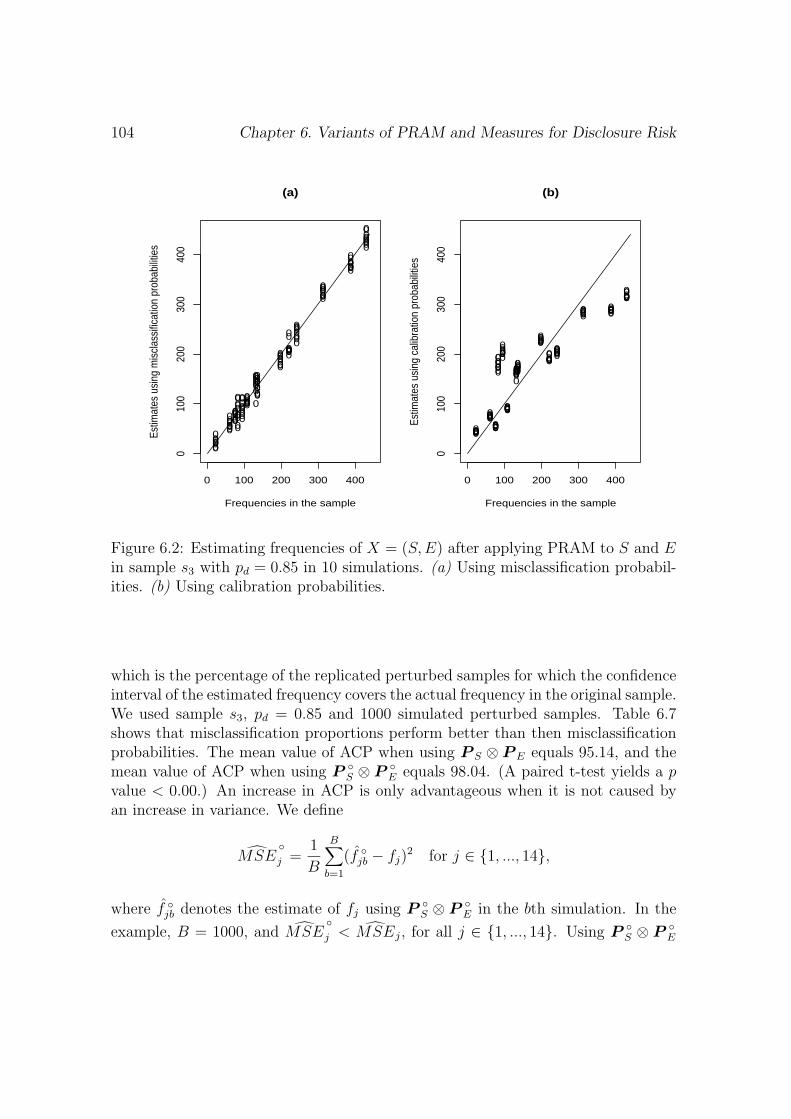
104 Chapter 6. Variants of PRAM and Measures for Disclosure Risk
0 100 200 300 400
010
020
030
040
0
(b)
Frequencies in the sample
Estim
ates
usi
ng c
alib
ratio
n pr
obab
ilitie
s0
0
00
0
0
0
0
00
0
0
0
0
0
0
00
0
0
0
0
0 0
0
0
0
0
0
0
00
0
0
00
0
0
0
0
0
0
0
0
00
0
0
0
0
00
0
0
0
0
0
0
00
0
0
0
0
00
0
0
0
0
0
0
00
0
0
0
0
00
0
0
0
0
0
0
0
0
0
0
0
0
00
0
0
0
0
0
0
00
0
0
00
00
0
0
0
0
0
0
00
0
0
0
0
00
0
0
0
0
0
0
00
0
0
0
0
0 0
0
0
0
0
0 100 200 300 400
010
020
030
040
0(a)
Frequencies in the sample
Estim
ates
usi
ng m
iscl
assi
ficat
ion
prob
abilit
ies
0
0
0
0
0
0
0
0
0
0
0
0
0
0
0
0
0
0
0
0
0
0
0
0
0
0
0
00
0
0
0
0
0
00
0
0
0
0
0
0
0
0
0
0
0
0
0
0
0
0
0
0
0
00
0
0
0
0
0
0
0
0
0
0
0
0
00
0
0
0
0
0
0
0
0
0
0
0
0
00
0
00
0
0
0
0
0
0
0
0
0
0
0
0
0
0
0
0
00
0
0
0
0
0
00
0
0
0
0
0
0
0
0
0
0
0
0
0
0
0
0
0
0
0
0
0
0
0
0
0
0
0
Figure 6.2: Estimating frequencies of X = (S,E) after applying PRAM to S and Ein sample s3 with pd = 0.85 in 10 simulations. (a) Using misclassification probabil-ities. (b) Using calibration probabilities.
which is the percentage of the replicated perturbed samples for which the confidenceinterval of the estimated frequency covers the actual frequency in the original sample.We used sample s3, pd = 0.85 and 1000 simulated perturbed samples. Table 6.7shows that misclassification proportions perform better than then misclassificationprobabilities. The mean value of ACP when using P S ⊗ P E equals 95.14, and themean value of ACP when using P
S ⊗ P E equals 98.04. (A paired t-test yields a p
value < 0.00.) An increase in ACP is only advantageous when it is not caused byan increase in variance. We define
MSEj =
1
B
B∑b=1
(f jb − fj)
2 for j ∈ 1, ..., 14,
where f jb denotes the estimate of fj using P
S ⊗ P E in the bth simulation. In the
example, B = 1000, and MSEj < MSEj, for all j ∈ 1, ..., 14. Using P
S ⊗ P E
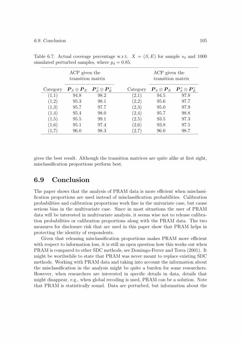
6.9. Conclusion 105
Table 6.7: Actual coverage percentage w.r.t. X = (S,E) for sample s3 and 1000simulated perturbed samples, where pd = 0.85.
ACP given thetransition matrix
ACP given thetransition matrix
Category P S ⊗ P E P S ⊗ P
E Category P S ⊗ P E P S ⊗ P
E
(1,1) 94.8 98.2 (2,1) 94.5 97.8(1,2) 95.3 98.1 (2,2) 95.6 97.7(1,3) 95.7 97.7 (2,3) 95.0 97.9(1,4) 95.4 98.0 (2,4) 95.7 98.8(1,5) 95.5 99.1 (2,5) 93.5 97.3(1,6) 95.1 97.4 (2,6) 93.8 97.5(1,7) 96.0 98.3 (2,7) 96.0 98.7
gives the best result. Although the transition matrices are quite alike at first sight,misclassification proportions perform best.
6.9 Conclusion
The paper shows that the analysis of PRAM data is more efficient when misclassi-fication proportions are used instead of misclassification probabilities. Calibrationprobabilities and calibration proportions work fine in the univariate case, but causeserious bias in the multivariate case. Since in most situations the user of PRAMdata will be interested in multivariate analysis, it seems wise not to release calibra-tion probabilities or calibration proportions along with the PRAM data. The twomeasures for disclosure risk that are used in this paper show that PRAM helps inprotecting the identity of respondents.
Given that releasing misclassification proportions makes PRAM more efficientwith respect to information loss, it is still an open question how this works out whenPRAM is compared to other SDC methods, see Domingo-Ferrer and Torra (2001). Itmight be worthwhile to state that PRAM was never meant to replace existing SDCmethods. Working with PRAM data and taking into account the information aboutthe misclassification in the analysis might be quite a burden for some researchers.However, when researchers are interested in specific details in data, details thatmight disappear, e.g., when global recoding is used, PRAM can be a solution. Notethat PRAM is statistically sound. Data are perturbed, but information about the
106 Chapter 6. Variants of PRAM and Measures for Disclosure Risk
perturbation can be used. Although estimates will have extra variance due to theperturbation, they will be unbiased.
Since the misclassification proportions provide more information about the origi-nal sample than the misclassification probabilities, one should consider the questionwhether providing these proportions increases the disclosure risk. Since the privacyprotection that is offered by PRAM is at the record level, we do not think thatdisclosure risk increases when misclassification proportions are released. With theseproportions, sample frequencies of the identifying variables can be deduced, butthese frequencies are not sensitive information. Note also that when one works withthe measures for disclosure risk discussed in Section 6.6, the risk does not changewhen misclassification proportions are released.
Appendix 6.A
The following shows that f =←−P XIE[F ∗|f ]. First note that IE[F ∗|f ] = P Xf and
that entries ←−p jk of←−P X are defined as ←−p jk = (pkjfj)(
∑Jj0=1 pkj0fj0)
−1 for k, j ∈1, ..., J. For each j ∈ 1, ..., J we have
(←−P XIE[F ∗|f ]
)(j) =
J∑k=1
←−p jk
(IE[F ∗|f ]
)(k)
=J∑
k=1
←−p jk
( J∑j0=1
pkj0fj0
)=
J∑k=1
pkjfj = fj,
since the columns of P X sum up to one. So f =←−P XP Xf and f is an eigenvector
of←−P XP X with eigenvalue 1.
In general,←−P X = P−1
X . To illustrate this, let R =←−P XP X . The entries of R are
rij =∑J
k=1←−p ikpkj, for i, j ∈ 1, ..., J. Assume that the entries of P X are all > 0
and that f j > 0, for j ∈ 1, ..., J. Then ←−p jk > 0, for j, k ∈ 1, ..., J and rij > 0,for i, j ∈ 1, ..., J. In this case, R is not the identity matrix and consequently←−P X = P−1
X . A more intuitive explanation is that←−P X changes when the survey
data change, whereas P X can be determined independently from the data and doesnot necessarily change when the data change. Therefore, it is always possible tocause
←−P X = P−1
X by changing the data.
Appendix 107
Appendix 6.B
The following derives the maximum likelihood properties of (6.3) and (6.8). Thereasoning is the same as in Hochberg (1977), but simpler, since in the PRAM situ-ation calibration probabilities do not have to be estimated. Also, we show that thereasoning applies both to (6.3) and to (6.8).
Assume that the frequency vector of independent X1, ...Xn is multinomially dis-tributed with parameters n and π = (π1, .., πJ)t, where πj > 0 for j ∈ 1, .., J, and∑J
j=1 πj = 1. Consider the transformation π∗ = Pπ, where P is a J × J transitionmatrix, i.e., columns sum up to one and pkj ≥ 0 for k, j ∈ 1, .., J. Assume thatP is nonsingular. Let the distribution of X∗ be given by IP (X∗ = k) = π∗
k, fork ∈ 1, .., J. It follows that the frequency vector of X∗
1 , X∗2 , ..., X
∗n is multinomially
distributed with parameters n and π∗. Indeed, π∗k = pk1π1 + ... + pkJπJ > 0 for
k ∈ 1, .., J and
J∑k=1
π∗k =
( J∑l=1
pl1
)π1 + ... +
( J∑l=1
plJ
)πJ = 1.
The likelihood L∗ for π∗ and observed x∗ = (x∗1, x
∗2, ..., x
∗n)t is well known. Let
f ∗ = (f ∗1 , f ∗
2 , ..., f ∗J )t denote the observed cell frequencies. The MLE is given by
π∗ = f ∗/n and has covariance matrix Ω = [Diag(π∗)−π∗(π∗)t]/n, where Diag(π∗)is the diagonal matrix with the diagonal entries given by the elements of π∗.
Next we can use the invariance property of maximum likelihood. Define thetransformation g(π∗) = P−1π∗. Since g is one-to-one, it follows from L∗(π∗|x∗) andπ = g(π∗) that the likelihood for π is given by L∗(g−1(π)|x∗) which is maximizedfor π = g(π∗) = P−1π∗. Consequently, when π ∈ (0, 1)J , it is the MLE. Since ghas a first order derivative, the covariance matrix of π can be obtained using thedelta-method, see, e.g., Agresti (2002, Chapter 14). We have ∂g(π∗)/∂π∗ = (P−1)t
and the covariance matrix of π is given by n−1P−1Ω(P−1)t.So with respect to (6.3), maximum likelihood properties are proven by taking
P = P X and obtaining π = g(π∗) = P−1X π∗. With respect to (6.8), the misclassi-
fication design is described by π =←−P Xπ∗, so P =
←−P
−1
X and the MLE is given by
π = g(π∗) =←−P Xπ∗.
Appendix 6.C
Let P kj denote the stochastic variable of the kj-th entry of P
X and Ckj the stochasticvariable of the kj-th cell in the cross-classification X∗ by X. It follows that Ckj has
108 Variants of PRAM and Measures for Disclosure Risk
a binomial distribution with parameters fj and pkj. Consequently, IE[P kj|f ] =
IE[Ckj/fj|f ] = fjpkj/fj = pkj and in expectation P X equals P X . Since Ck1j1 and
Ck2j2 are independent given f , it follows that IE[P k1j1
P k2j2
|f ] = pk1j1pk2j2 . So inexpectation, P
X1⊗ P
X equals P X1 ⊗ P X2 .
We define←−P
jk = Ckj/(F
∗k + ε) where ε is a small positive value. Using the delta
method, see, e.g., Rice (1995, Section 4.6), we obtain
IE[←−P
jk|f ] ≈ IE[Ckj|f ]
IE[F ∗k |f ]
+1
IE[F ∗k |f ]2
(V [F ∗
k |f ]IE[Ckj|f ]
IE[F ∗k |f ]
− ρ√
V [Ckj|f ]V [F ∗k |f ]
),
where IE[Ckj|f ] = fjpkj and ρ is the correlation between Ckj and F ∗k . From this we
see that the difference between IE[←−P
jk|f ] and ←−p jk will be small when V [F ∗
k |f ] issmall and IE[F ∗
k |f ] is large.
References
Agresti, A. (1996). An Introduction to Categorical Data Analysis, New York: Wi-ley.
Agresti, A. (2002). Categorical Data Analysis, Second Edition, New York: Wiley.
Assakul, K., and Proctor, C.H. (1967). Testing independence in two-way contin-gency tables with data subject to misclassification, Psychometrika 32, 67-76.
Barndorff-Nielsen, O. (1982). Exponential families, Encyclopedia of Statistical Sci-ences (S. Kotz and N.L. Norman, eds), New York: Wiley.
Bethlehem, J.G., Keller, W.J., and Pannekoek, J. (1990). Disclosure control ofmicrodata, Journal of the American Statistical Association 85, 38-45.
Bishop, Y.M.M., Fienberg, S.E., and Holland, P.W. (1975). Discrete MultivariateAnalysis, Cambridge: MIT Press.
Bergsma, W.P., and Rudas, T. (2002). Marginal models for categorical data, TheAnnals of Statistics 30, 140-159.
Boeije, H., and Lensvelt-Mulders, G. (2002). Honest by chance: a qualitative in-terview study to clarify respondents’ (non-)compliance with computer-assistedrandomized response, Bulletin de Methodologie Sociologique 75, 24-39.
Bourke, P.D. and Moran, M.A. (1988). Estimating proportions from randomizedresponse data using the EM algorithm, Journal of the American StatisticalAssociation 83, 964-968.
Boruch, R.F. (1971). Assuring confidentiality of responses in social research: anote on strategies, The American Sociologist 6, 308-311.
Chaudhuri, A., and Mukerjee, R. (1988). Randomized Response: Theory and Tech-niques, New York: Marcel Dekker.
Chen, T.T. (1989). A review of methods for misclassified categorical data in epi-demiology, Statistics in Medicine 8, 1095-1106.
109
110 References
Copeland, K.T., Checkoway, H., McMichael, A. J., and Holbrook, R. H. (1977).Bias due to misclassification in the estimation of relative risk, American Jour-nal of Epidemiology 105, 488-495.
Dempster, A. P., Laird, N.M. and Rubin, D.B. (1977). Maximum likelihood fromincomplete data via the EM algorithm, Journal of the Royal Statistical SocietyB 39, 1-38.
De Wolf, P.-P., Gouweleeuw, J.M., Kooiman, P., and Willenborg, L.C.R.J (1997).Reflections on PRAM. Research paper no. 9742, Voorburg/ Heerlen: StatisticsNetherlands.
Domingo-Ferrer, J., and Torra, V. (2001). A quantitative comparison of disclosurecontrol methods for microdata, In Confidentiality, Disclosure, and Data Ac-cess, Theory and Practical Application for Statistical Agencies, (P. Doyle, J.Lane, L. Zayatz, and J. Theeuwes, eds.) Amsterdam: North-Holland.
Efron, B, and Tibshirani, R.J (1993). An Introduction to the Bootstrap, New York:Chapman and Hall.
Elamir, E.A.H., and Skinner, C.J. (2003). Disclosure risk assessment for microdata,the treatment of measurement Error, manuscript.
Elffers, E., Van der Heijden, P.G.M., and Hezemans, M. (2003). Explaining regu-latory non-compliance: a survey study of rule transgression for two Dutch in-strumental laws, applying the randomized response method, Journal of Quan-titative Criminology 19, 409-439.
Evfimievski, A., Srikant, R., Agrawal, R., and Gehrke (2002) Privacy preservingmining of association rules, in Proceedings of the 8th ACM SIGKDD Inter-national Conference on Knowledge Discovery in Databases and Data Mining,Edmonton, Alberta, Canada, 2002, 217-228.
Fienberg, S.E. (1980). The Analysis of Cross-Classified Categorical Data, Cam-bridge, MA: MIT Press.
Fox, J.A., and Tracy, P.E. (1986). Randomized Response: A Method for SensitiveSurveys, Newbury Park: Sage.
Gelman, A., Meng, X.L., and Stern, H. (1996). Posterior predictive assessment ofmodel fitness via realized discrepancies, Statistica Sinica 6, 733-807.
111
Goodman, L.A. (1973). The analysis of multidimensional contingency tables whensome variables are posterior to others: a modified path analysis approach,Biometrika 60, 179-192.
Goodman, L.A. (1974). Explanatory latent-structure analysis using both identifi-able and unidentifiable models, Biometrika 61, 251-231.
Gouweleeuw, J.M., Kooiman, P., Willenborg, L.C.R.J., and De Wolf, P.-P. (1998).Post randomisation for statistical disclosure control: theory and implementa-tion, Journal of Official Statistics 14, 463-478.
Greenland, S. (1980). The effect of misclassification in the presence of covariates,American Journal of Epidemiology 112, 564-569.
Greenland, S. (1988). Variance estimation for epidemiologic effect estimates undermisclassification, Statistics in Medicine 7, 745-757.
Haberman, S.J. (1977). Product models for frequency tables involving indirectobservation, The Annals of Statistics 5, 1124-1147.
Haberman, S.J. (1979). Analysis of Qualitative Data: New Developments (Vol.2),New York: Academic Press.
Hagenaars, J.A. (1993). Loglinear Models With Latent Variables, Newbury Park:Sage.
Heinen, T. (1996). Latent Class and Discrete Latent Trait Models: Similarities andDifferences, Thousand Oaks: Sage Publications.
Hochberg, Y. (1977). On the use of double sampling schemes in analyzing cate-gorical data with misclassification errors, Journal of the American StatisticalAssociation 72, 914-921.
Kooiman, P., Willenborg, L.C.R.J., and Gouweleeuw, J.M. (1997). PRAM: amethod for disclosure limitation of microdata, Research paper no. 9705, Voor-burg/Heerlen: Statistics Netherlands.
Korn, E.L. (1981). Hierarchical log-linear models not preserved by classificationerror, Journal of the American Statistical Association 76, 110-113.
Kuha, J., and Skinner, C. (1997). Categorical data analysis and misclassification, inSurvey Measurement and Process Quality, (L. Lyberg, P. Biemer, M. Collins,E. De Leeuw, C. Dippo, N. Schwarz, and D. Trewin, eds.), New York: Wiley.
112 References
Kuk, A.Y.C. (1990). Asking sensitive questions indirectly. Biometrika 77, 436-438.
Lindsay, B.G. (1995). Mixture Models: Theory, Geometry and Applications, NSF-CBMS Regional Conference Series in Probability and Statistics Vol. 5, Hay-ward, California: Institute of Mathematical Statistics.
Little, J.A., and Rubin D.B. (2002). Statistical Analysis With Missing Data, SecondEdition, New York: Wiley.
Lucy, L.B. (1974). An iterative technique for the rectification of observed distri-butions, The Astronomical Journal 79, 745-754.
Maddala, G.S. (1983). Limited Dependent and Qualitative Variables in Economet-rics, Cambridge: Cambridge University Press.
Magder, L. S., and Hughes, J. P. (1997). Logistic regression when the outcome ismeasured with uncertainty, American Journal of Epidemiology 146, 195-203.
McLachlan, G. F., and Krishnan, T. (1997). The EM Algorithm and Extensions,New York: Wiley.
Mood, A.M., Graybill, F.A., and Boes, D.C. (1985). Introduction to the theory ofStatistics, Auckland: McGraw-Hill.
Moors, J.J.A. (1981). Inadmissibility of linearly invariant estimators in truncatedparameter spaces, Journal of the American Statistical Association 76, 910-915.
Moriarty, M., and Wiseman, F. (1976). On the choice of a randomization techniquewith the randomized response model, Proceedings of the social statistics sectionof the American Statistical Association, 624-626.
Mote, V.L., and Anderson, R.L. (1965). An investigation of the effect of mis-classification on the properties of χ2-tests in the analysis of categorical data,Biometrika 52, 95-109.
Rice, J.A. (1995). Mathematical Statistics and Data Analysis, Belmont: DuxburyPress.
Rosenberg, M.J. (1979). Multivariate analysis by a randomized response techniquefor statistical disclosure control, Ph.D. Dissertation, University of Michigan.
113
Rosenberg, M.J. (1980). Categorical data analysis by a randomized response tech-nique for statistical disclosure control, Proceedings of the Survey ResearchMethods Section, American Statistical Association, 311-318.
Rubin, D.B. (1976). Inference and missing data, Biometrika 63, 581-592.
Schafer J.L.(1997). Analysis of Incomplete Multivariate Data, London: Chapmanand Hall.
Schwartz, J.E. (1985). The neglected problem of measurement error in categoricaldata, Sociological Methods and Research 13, 435-466.
Singh, J. (1976). A note on randomized response techniques, Proceedings of thesocial statistics section of the American Statistical Association, 772.
Skinner, C.J., and Elliot, M.J. (2002). A measure of disclosure risk for microdata,Journal of the Royal Statistical Society B 64, 855-867.
Spiegelman, D., Rosner B., and Logan, R. (2000). Estimation and inference forlogistic regression with covariate misclassification and measurement error inmain study/validation study designs, Journal of the American Statistical As-sociation 95, 51-61.
Van den Hout, A. (1999) The Analysis of Data Perturbed by PRAM, WBBM ReportSeries 45, Delft: Delft University Press.
Van den Hout, A., and Van der Heijden, P.G.M (2002). Randomized response,statistical disclosure control and misclassification: a review, International Sta-tistical Review 70, 269-288.
Van den Hout, A., and Van der Heijden, P.G.M (2004). The analysis of multi-variate misclassified data with special attention to randomized response data,Sociological Methods and Research 32, 310-336.
Van der Heijden, P.G.M, and Van Gils, G. (1996). Some logistic regression modelsfor randomized response data, Proceedings of the eleventh international work-shop on statistical modelling, (A. Forcina, G. M. Marchetti, R. Hatzinger andG. Falmacci eds.).
Van der Heijden, P.G.M., Van Gils, G., Bouts, J., and Hox, J.J. (2000). A compar-ison of randomized response, computer-assisted self-interview, and face-to-facedirect questioning, Sociological Methods and Research 28, 505-537.
114 References
Van Gils, G., Van der Heijden, P.G.M., Laudy, O., Ross, R (2003). Regelovertred-ing in de sociale zekerheid, Den Haag: Ministerie van Social Zaken en Werkgele-genheid. (In Dutch)
Van Gils, G., Van der Heijden, P.G.M., and Rosebeek, A. (2001). Onderzoek naarregelovertreding. Resultaten ABW, WAO en WW. Amsterdam: NIPO. (InDutch)
Vermunt, J.K. (1997). LEM: a general program for the analysis of categorical data,user’s manual, Tilburg: Tilburg University.
Warner, S.L. (1965). Randomized response: a survey technique for eliminatinganswer bias, Journal of the American Statistical Association 60, 63-69.
Warner, S.L. (1971). The linear randomized response model, Journal of the Amer-ican Statistical Association 66, 884-888.
Willenborg, L.C.R.J. (2000). Optimality models for PRAM, Proceedings in Com-putational Statistics (J.G. Bethlehem, J.G., and Van der Heijden, P.G.M.,eds.), Heidelberg: Physica-Verlag.
Willenborg, L.C.R.J., and De Waal, T. (2001). Elements of Statistical DisclosureControl, New York: Springer.
Samenvatting
Dit boek gaat over de analyse van randomized response-data en over de ana-lyse van post randomization-data. Randomized response (RR) is een methodedie wordt gebruikt in onderzoek naar sensitieve items (Warner 1965). Voor-beelden van sensitieve items zijn items over fraude, seksueel gedrag of alco-holgebruik. In een situatie waarin vragen over sensitieve items onmiddellijkworden gesteld, kan het zijn dat respondenten niet naar waarheid antwoordenvanwege privacy-overwegingen. De RR-methode zorgt er voor dat de privacywordt gewaarborgd, omdat het antwoord van de respondent op een sensitievevraag deels wordt bepaald door een kansmechanisme. De RR-methode is inNederland toegepast, zie bijvoorbeeld Van Gils, Van der Heijden, Laudy enRoss (2003), en Elffers, Van der Heijden en Hezemans (2003).
Een voorbeeld van een RR-methode is de methode van Boruch (1971). Steldat het antwoord op de sensitieve vraag ja of nee is. In Boruch’s methodekrijgt de respondent twee dobbelstenen. De sensitieve vraag wordt gesteld envoordat de respondent antwoordt, gooit hij met de dobbelstenen. Afhankelijkvan het aantal ogen dat wordt gegooid, bepaalt de respondent zijn antwoord.Als het aantal ogen 2, 3 of 4 is, antwoordt de respondent ja. Als het aantalogen 5, 6, 7, 8, 9, of 10 is, antwoordt de respondent naar waarheid. Als hetaantal ogen 11 of 12 is, antwoordt de respondent nee. In deze methode is hetkansmechanisme het gebruik van de dobbelstenen. Het mechanisme beschermtde privacy, want het aantal ogen dat wordt gegooid, wordt voor de interviewerverborgen gehouden. Omdat we het kansmechanisme goed kennen, kunnen weer rekening mee houden in de analyse van de geobserveerde antwoorden.
De post randomization methode (PRAM) kan worden gezien als een specialetoepassing van de RR-methode (Kooiman, Willenborg en Gouweleeuw 1997).PRAM beschermt data die al is verzameld en die wordt vrijgegeven voor on-derzoekers buiten het instituut dat de data verzamelde. Ook in deze situatie
115
116 Samenvatting
is de bescherming van de privacy nodig. Het kansmechanisme wordt bij PRAMuitgevoerd door een computer. De verstoorde data worden samen met infor-matie over het kansmechanisme, en onder bepaalde voorwaarden, vrijgegeven.
Dit boek beschrijft de verstoring door RR of PRAM met behulp van eenmisclassificatie model. Het eerste hoofdstuk introduceert RR en PRAM.
Hoofdstuk 2 gaat over het schatten van proporties en over het meten vanafhankelijkheid. Met de methoden in dit hoofdstuk kunnen vragen wordenbeantwoord als bijvoorbeeld: Hoeveel mensen hebben er gefraudeerd? en Isfraude plegen afhankelijk van de indeling man/vrouw? Omdat er in het schat-ten rekening moet worden gehouden met het kansmechanisme, is de analysevan de gegevens anders dan in een standaardsituatie zonder RR of PRAM.
Hoofdstuk 3 behandelt het fitten van loglineare modellen voor RR-data ofPRAM-data. Loglineare modellen beschrijven complexe, meer-dimensionalestructuren voor afhankelijkheid. Met de methode in dit hoofdstuk kan bijvoor-beeld de volgende vraag worden beantwoord: Is fraude plegen afhankelijk vanzowel de indeling man/ vrouw alsook van de grootte van de woonplaats?
In hoofdstuk 4 wordt een specifiek onderzoek beschreven waarin sommigerespondenten via RR vragen beantwoordden en andere respondenten directantwoordden. Opnieuw worden loglineare modellen gefit, maar nu wordt erook rekening gehouden met het feit dat niet alle respondenten de RR-methodegebruiken.
Regressiemodellen worden geschat in hoofdstuk 5. In dit hoofdstuk wordtde situatie beschreven waarin RR-variabelen onafhankelijke variabelen in eenstandaard lineair regressiemodel zijn. Een situatie als deze kan ontstaan wan-neer seksueel gedrag met behulp van RR wordt gemeten en het verband meteen afhankelijke variabele wordt onderzocht door een lineair regressiemodel.
Hoofdstuk 6 gaat over PRAM en over de informatie over het kansmechanismedie wordt meegegeven met de verstoorde data. Omdat PRAM wordt toegepastmet behulp van een computer op bestaande data, zijn er meer mogelijkhedenvoor het verstrekken van informatie over het kansmechanisme dan bij RR.Ook worden er in dit hoofdstuk maten gegeven voor de privacybeschermingwanneer PRAM is toegepast.
Het boek laat zien dat, gegeven een aantal assumpties, de analyse van RR-data zeer goed mogelijk is. Het boek laat ook zien, vooral in hoofdstuk 3,dat die assumpties niet altijd houdbaar zijn en dat in sommige gevallen verderonderzoek nodig is voor het beter modelleren van RR-data.

Curriculum Vitae
Ardo van den Hout was born in Dirksland, the Netherlands, on March 8, 1968.After completing secondary school (VWO) in 1989, he started studying philos-ophy and mathematics at the University of Nijmegen. In 1996, he graduated inphilosophy (cum laude), and in 1997 he graduated in mathematics. From 1997to 1999, he followed a two-year post-Master’s program at the Department ofMathematics and Computer Science at Delft University, which included a one-year work placement at Statistic Netherlands in Voorburg. In 2000, he startedhis Ph.D. research which was a joint project of Statistic Netherlands and theDepartment of Methodology and Statistics of the Faculty of Social Sciences atUtrecht University. Currently, he is employed as a postdoc researcher at theDepartment of Methodology and Statistics at Utrecht University.