Appendix F: File Organizations and Indexeswps.aw.com/wps/media/objects/7095/7265991/appendices/AppendixF… · Chapter 18 require the selection of appropriate file organizations and

APPENDIX

F File Organizations and Indexes

Objectives

In this appendix you will learn:

• The distinction between primary and secondary storage.

• The meanings of file organization and access method.

• How heap files are organized.

• How sequential files are organized.

• How hash files are organized.

• What an index is and how it can be used to speed up database retrievals.

• The distinction between a primary, secondary, and clustered indexes.

• How indexed sequential files are organized.

• How multilevel indexes are organized.

• How B+-trees are organized.

• How bitmap indexes are organized.

• How join indexes are organized.

• How indexed clusters and hash clusters are organized.

• How to select an appropriate file organization.

Steps 4.2 and 4.3 of the physical database design methodology presented inChapter 18 require the selection of appropriate file organizations and indexes forthe base relations that have been created to represent the part of the enterprisebeing modeled. In this appendix we introduce the main concepts regarding thephysical storage of the database on secondary storage devices such as magneticdisks and optical disks. The computer’s primary storage—that is, main memory—is inappropriate for storing the database. Although the access times for primarystorage are much faster than secondary storage, primary storage is not large orreliable enough to store the quantity of data that a typical database might require.Because the data stored in primary storage disappears when power is lost, we referto primary storage as volatile storage. In contrast, the data on secondary storagepersists through power loss, and is consequently referred to as nonvolatile storage.

F-1

F-2 | Appendix F File Organizations and Indexes

In addition, the cost of storage per unit of data is an order of magnitude greaterfor primary storage than for disk storage.

Structure of this Appendix In Section F.1 we introduce the basicconcepts of physical storage. In Sections F.2–F.4 we discuss the main types offile organization: heap (unordered), sequential (ordered), and hash files. InSection F.5 we discuss how indexes can be used to improve the performanceof database retrievals. In particular, we examine indexed sequential files,multilevel indexes, B+-trees, bitmap indexes, and join indexes. Finally, inSection F.6, we provide guidelines for selecting file organizations. Theexamples in this chapter are drawn from the DreamHome case studydocumented in Section 11.4 and Appendix A.

F.1 Basic Concepts

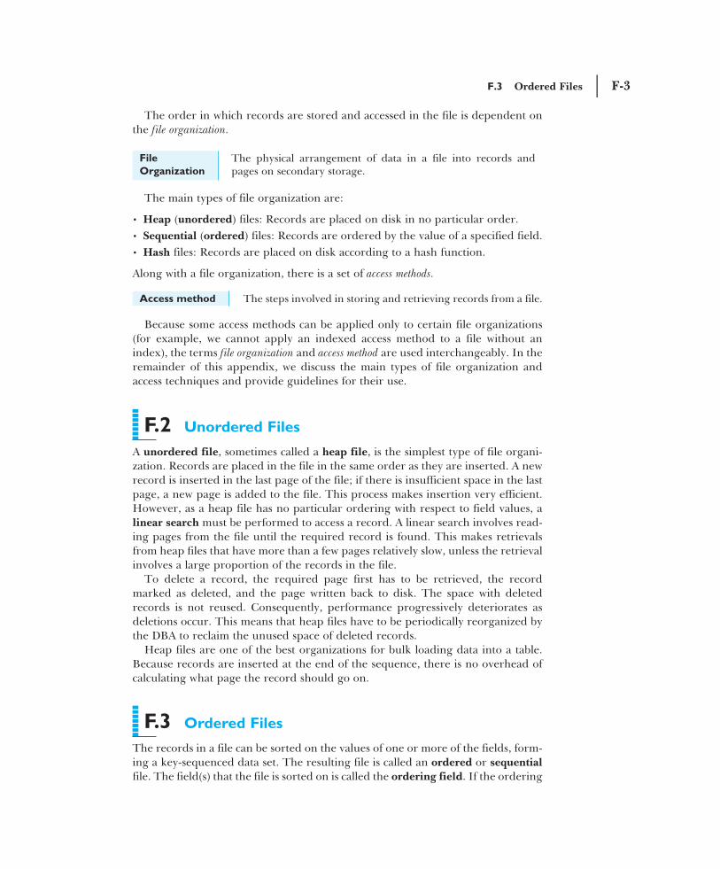
The database on secondary storage is organized into one or more files; each fileconsists of one or more records and each record consists of one or more fields.Typically, a record corresponds to an entity and a field to an attribute. Considerthe reduced Staff relation from the DreamHome case study shown in Figure F.1.

We may expect each tuple in this relation to map to a record in the operatingsystem file that holds the Staff relation. Each field in a record would store oneattribute value from the Staff relation. When a user requests a tuple from theDBMS—for example, Staff tuple SG37—the DBMS maps this logical record on toa physical record and retrieves the physical record into the DBMS buffers in pri-mary storage using the operating system file access routines.

The physical record is the unit of transfer between disk and primary storage, andvice versa. Generally, a physical record consists of more than one logical record,although depending on size, a logical record can correspond to one physical record.It is even possible for a large logical record to span more than one physical record.The terms block and page are sometimes used in place of physical record. In theremainder of this appendix we use the term “page.” For example, the Staff tuplesin Figure F.1 may be stored on two pages, as shown in Figure F.2.

Figure F.1 Reduced Staff relation

from DreamHome case study. Figure F.2 Storage of Staff relation in pages.

F.3 Ordered Files | F-3

The order in which records are stored and accessed in the file is dependent onthe file organization.

File

Organization

The physical arrangement of data in a file into records andpages on secondary storage.

The main types of file organization are:

• Heap (unordered) files: Records are placed on disk in no particular order.• Sequential (ordered) files: Records are ordered by the value of a specified field.• Hash files: Records are placed on disk according to a hash function.

Along with a file organization, there is a set of access methods.

Access method The steps involved in storing and retrieving records from a file.

Because some access methods can be applied only to certain file organizations(for example, we cannot apply an indexed access method to a file without anindex), the terms file organization and access method are used interchangeably. In theremainder of this appendix, we discuss the main types of file organization andaccess techniques and provide guidelines for their use.

F.2 Unordered Files

A unordered file, sometimes called a heap file, is the simplest type of file organi-zation. Records are placed in the file in the same order as they are inserted. A newrecord is inserted in the last page of the file; if there is insufficient space in the lastpage, a new page is added to the file. This process makes insertion very efficient.However, as a heap file has no particular ordering with respect to field values, alinear search must be performed to access a record. A linear search involves read-ing pages from the file until the required record is found. This makes retrievalsfrom heap files that have more than a few pages relatively slow, unless the retrievalinvolves a large proportion of the records in the file.

To delete a record, the required page first has to be retrieved, the recordmarked as deleted, and the page written back to disk. The space with deletedrecords is not reused. Consequently, performance progressively deteriorates asdeletions occur. This means that heap files have to be periodically reorganized bythe DBA to reclaim the unused space of deleted records.

Heap files are one of the best organizations for bulk loading data into a table.Because records are inserted at the end of the sequence, there is no overhead ofcalculating what page the record should go on.

F.3 Ordered Files

The records in a file can be sorted on the values of one or more of the fields, form-ing a key-sequenced data set. The resulting file is called an ordered or sequentialfile. The field(s) that the file is sorted on is called the ordering field. If the ordering


field is also a key of the file, and therefore guaranteed to have a unique value ineach record, the field is also called the ordering key for the file. For example, con-sider the following SQL query:

SELECT *FROM Staff

ORDER BY staffNo;

If the tuples of the Staff relation are already ordered according to the orderingfield staffNo, it should be possible to reduce the execution time for the query, as nosorting is necessary. (Although in Section 4.2 we stated that tuples are unordered,this applies as an external (logical) property, not as an implementation or physicalproperty. There will always be a first record, second record, and nth record.) If thetuples are ordered on staffNo, under certain conditions we can use a binary searchto execute queries that involve a search condition based on staffNo. For example,consider the following SQL query:

SELECT *FROM Staff

WHERE staffNo = ‘SG37’;

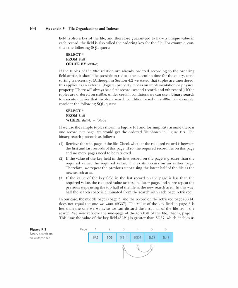
If we use the sample tuples shown in Figure F.1 and for simplicity assume there isone record per page, we would get the ordered file shown in Figure F.3. Thebinary search proceeds as follows:

(1) Retrieve the mid-page of the file. Check whether the required record is betweenthe first and last records of this page. If so, the required record lies on this pageand no more pages need to be retrieved.

(2) If the value of the key field in the first record on the page is greater than therequired value, the required value, if it exists, occurs on an earlier page.Therefore, we repeat the previous steps using the lower half of the file as thenew search area.

(3) If the value of the key field in the last record on the page is less than therequired value, the required value occurs on a later page, and so we repeat theprevious steps using the top half of the file as the new search area. In this way,half the search space is eliminated from the search with each page retrieved.

In our case, the middle page is page 3, and the record on the retrieved page (SG14)does not equal the one we want (SG37). The value of the key field in page 3 is less than the one we want, so we can discard the first half of the file from thesearch. We now retrieve the mid-page of the top half of the file, that is, page 5.This time the value of the key field (SL21) is greater than SG37, which enables us

Figure F.3

Binary search on

an ordered file.

F.4 Hash Files | F-5

to discard the top half of this search space. We now retrieve the mid-page of theremaining search space, that is, page 4, which is the record we want.

In general, the binary search is more efficient than a linear search. However,binary search is applied more frequently to data in primary storage than secondarystorage.

Inserting and deleting records in a sorted file are problematic because the orderof records has to be maintained. To insert a new record, we must find the correctposition in the ordering for the record and then find space to insert it. If there issufficient space in the required page for the new record, then the single page canbe reordered and written back to disk. If this is not the case, then it would be nec-essary to move one or more records on to the next page. Again, the next page mayhave no free space and the records on this page must be moved, and so on.

Inserting a record near the start of a large file could be very time-consuming.One solution is to create a temporary unsorted file, called an overflow (ortransaction) file. Insertions are added to the overflow file, and periodically, the over-flow file is merged with the main sorted file. This makes insertions very efficient,but has a detrimental effect on retrievals. If the record is not found during thebinary search, the overflow file has to be searched linearly. Inversely, to delete arecord we must reorganize the records to remove the now free slot.

Ordered files are rarely used for database storage unless a primary index isadded to the file (see Section F.5.1).

F.4 Hash Files

In a hash file, records do not have to be written sequentially to the file. Instead, ahash function calculates the address of the page in which the record is to be storedbased on one or more fields in the record. The base field is called the hash field,or if the field is also a key field of the file, it is called the hash key. Records in ahash file will appear to be randomly distributed across the available file space. Forthis reason, hash files are sometimes called random, or direct, files.

The hash function is chosen so that records are as evenly distributed as possiblethroughout the file. One technique, called folding, applies an arithmetic function,such as addition, to different parts of the hash field. Character strings are con-verted into integers before the function is applied using some type of code, suchas alphabetic position or ASCII values. For example, we could take the first twocharacters of the staff number, staffNo, convert them to an integer value, then addthis value to the remaining digits of the field. The resulting sum is used as theaddress of the disk page in which the record is stored. An alternative, more popu-lar technique, is the division-remainder hashing. This technique uses the MOD func-tion, which takes the field value, divides it by some predetermined integer value,and uses the remainder of this division as the disk address.

The problem with most hashing functions is that they do not guarantee a uniqueaddress, because the number of possible values a hash field can take is typicallymuch larger than the number of available addresses for records. Each address gen-erated by a hashing function corresponds to a page, or bucket, with slots for mul-tiple records. Within a bucket, records are placed in order of arrival. When thesame address is generated for two or more records, a collision is said to have


occurred (the records are called synonyms). In this situation, we must insert thenew record in another position, because its hash address is occupied. Collisionmanagement complicates hash file management and degrades overall perfor-mance. There are several techniques that can be used to manage collisions:

• open addressing• unchained overflow• chained overflow• multiple hashing

Open addressing

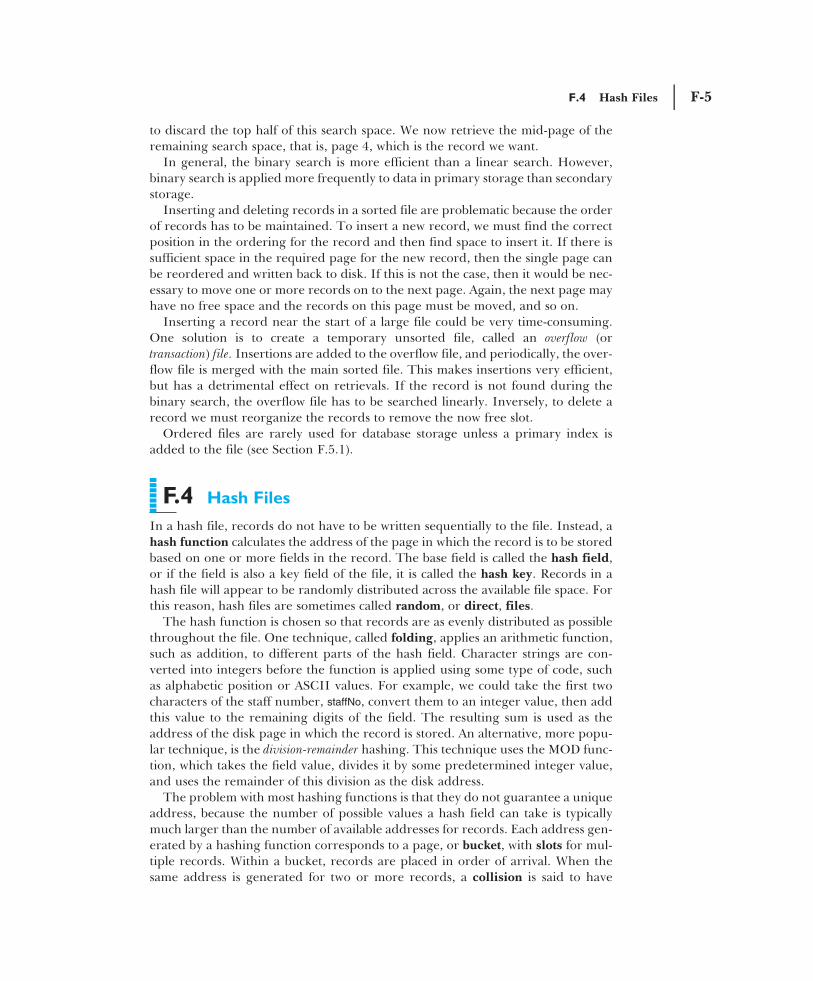
If a collision occurs, the system performs a linear search to find the first availableslot to insert the new record. When the last bucket has been searched, the systemstarts back at the first bucket. Searching for a record employs the same techniqueused to store a record, except that the record is considered not to exist when anunused slot is encountered before the record has been located. For example,assume we have a trivial hash function that takes the digits of the staff numberMOD 3, as shown in Figure F.4. Each bucket has two slots and staff records SG5and SG14 hash to bucket 2. When record SL41 is inserted, the hash function gen-erates an address corresponding to bucket 2. As there are no free slots in bucket 2,it searches for the first free slot, which it finds in bucket 1, after looping back andsearching bucket 0.

Unchained overflow

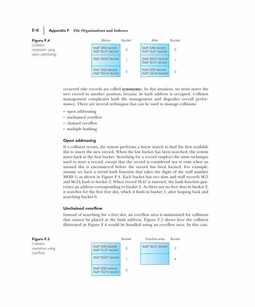
Instead of searching for a free slot, an overflow area is maintained for collisionsthat cannot be placed at the hash address. Figure F.5 shows how the collisionillustrated in Figure F.4 would be handled using an overflow area. In this case,

Figure F.4

Collision

resolution using

open addressing.

Figure F.5

Collision

resolution using

overflow.

instead of searching for a free slot for record SL41, the record is placed in theoverflow area. At first sight, this may appear not to offer much performanceimprovement. However, using open addressing, collisions are located in the firstfree slot, potentially causing additional collisions in the future with records thathash to the address of the free slot. Thus, the number of collisions that occur isincreased and performance is degraded. On the other hand, if we can minimizethe number of collisions, it will be faster to perform a linear search on a smalleroverflow area.

Chained overflow

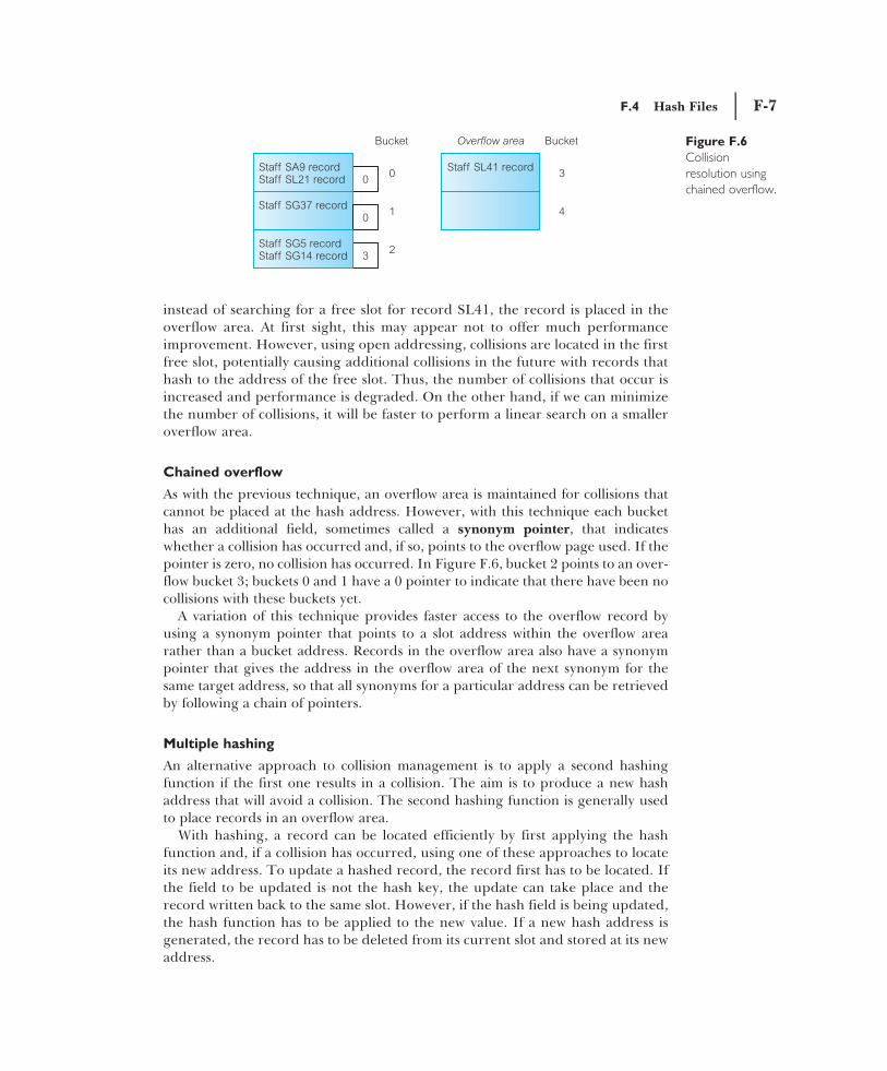
As with the previous technique, an overflow area is maintained for collisions thatcannot be placed at the hash address. However, with this technique each buckethas an additional field, sometimes called a synonym pointer, that indicateswhether a collision has occurred and, if so, points to the overflow page used. If thepointer is zero, no collision has occurred. In Figure F.6, bucket 2 points to an over-flow bucket 3; buckets 0 and 1 have a 0 pointer to indicate that there have been nocollisions with these buckets yet.

A variation of this technique provides faster access to the overflow record byusing a synonym pointer that points to a slot address within the overflow arearather than a bucket address. Records in the overflow area also have a synonympointer that gives the address in the overflow area of the next synonym for thesame target address, so that all synonyms for a particular address can be retrievedby following a chain of pointers.

Multiple hashing

An alternative approach to collision management is to apply a second hashingfunction if the first one results in a collision. The aim is to produce a new hashaddress that will avoid a collision. The second hashing function is generally usedto place records in an overflow area.

With hashing, a record can be located efficiently by first applying the hashfunction and, if a collision has occurred, using one of these approaches to locateits new address. To update a hashed record, the record first has to be located. Ifthe field to be updated is not the hash key, the update can take place and therecord written back to the same slot. However, if the hash field is being updated,the hash function has to be applied to the new value. If a new hash address isgenerated, the record has to be deleted from its current slot and stored at its newaddress.

Figure F.6

Collision

resolution using

chained overflow.

F.4 Hash Files | F-7


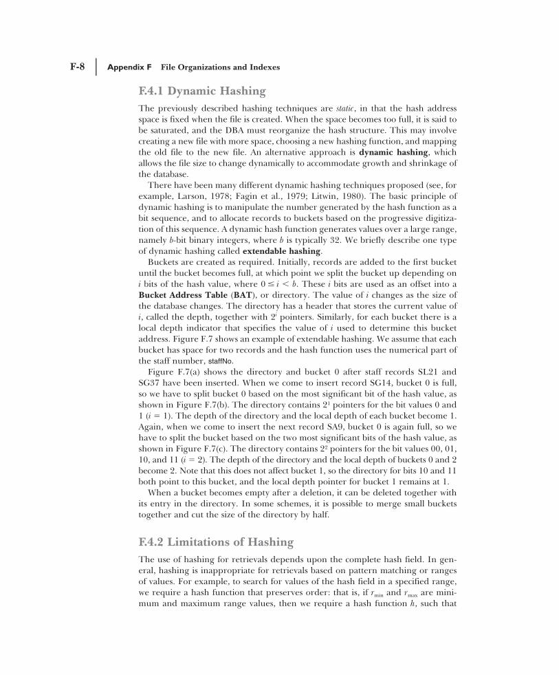
F.4.1 Dynamic HashingThe previously described hashing techniques are static, in that the hash addressspace is fixed when the file is created. When the space becomes too full, it is said tobe saturated, and the DBA must reorganize the hash structure. This may involvecreating a new file with more space, choosing a new hashing function, and mappingthe old file to the new file. An alternative approach is dynamic hashing, whichallows the file size to change dynamically to accommodate growth and shrinkage ofthe database.

There have been many different dynamic hashing techniques proposed (see, forexample, Larson, 1978; Fagin et al., 1979; Litwin, 1980). The basic principle ofdynamic hashing is to manipulate the number generated by the hash function as abit sequence, and to allocate records to buckets based on the progressive digitiza-tion of this sequence. A dynamic hash function generates values over a large range,namely b-bit binary integers, where b is typically 32. We briefly describe one typeof dynamic hashing called extendable hashing.

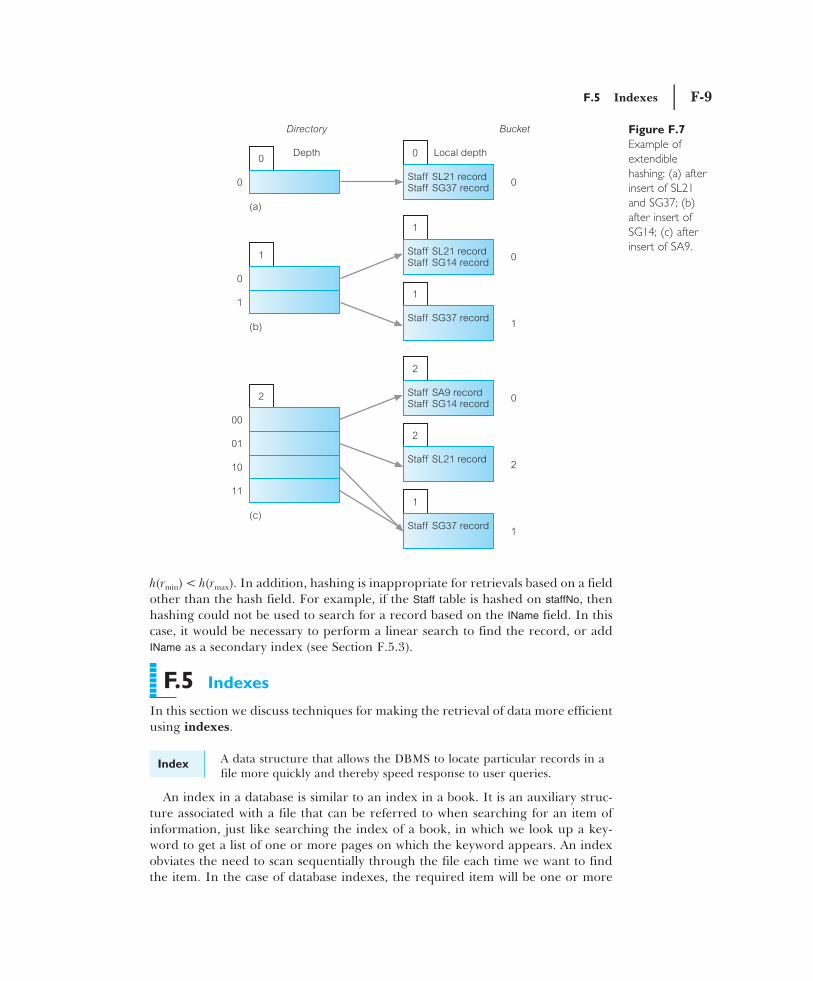
Buckets are created as required. Initially, records are added to the first bucketuntil the bucket becomes full, at which point we split the bucket up depending oni bits of the hash value, where 0 i � b. These i bits are used as an offset into aBucket Address Table (BAT), or directory. The value of i changes as the size ofthe database changes. The directory has a header that stores the current value ofi, called the depth, together with 2i pointers. Similarly, for each bucket there is alocal depth indicator that specifies the value of i used to determine this bucketaddress. Figure F.7 shows an example of extendable hashing. We assume that eachbucket has space for two records and the hash function uses the numerical part ofthe staff number, staffNo.

Figure F.7(a) shows the directory and bucket 0 after staff records SL21 andSG37 have been inserted. When we come to insert record SG14, bucket 0 is full,so we have to split bucket 0 based on the most significant bit of the hash value, asshown in Figure F.7(b). The directory contains 21 pointers for the bit values 0 and1 (i � 1). The depth of the directory and the local depth of each bucket become 1.Again, when we come to insert the next record SA9, bucket 0 is again full, so wehave to split the bucket based on the two most significant bits of the hash value, asshown in Figure F.7(c). The directory contains 22 pointers for the bit values 00, 01,10, and 11 (i � 2). The depth of the directory and the local depth of buckets 0 and 2become 2. Note that this does not affect bucket 1, so the directory for bits 10 and 11both point to this bucket, and the local depth pointer for bucket 1 remains at 1.

When a bucket becomes empty after a deletion, it can be deleted together withits entry in the directory. In some schemes, it is possible to merge small bucketstogether and cut the size of the directory by half.

F.4.2 Limitations of HashingThe use of hashing for retrievals depends upon the complete hash field. In gen-eral, hashing is inappropriate for retrievals based on pattern matching or rangesof values. For example, to search for values of the hash field in a specified range,we require a hash function that preserves order: that is, if rmin and rmax are mini-mum and maximum range values, then we require a hash function h, such that

…

F.5 Indexes | F-9

h(rmin) < h(rmax). In addition, hashing is inappropriate for retrievals based on a fieldother than the hash field. For example, if the Staff table is hashed on staffNo, thenhashing could not be used to search for a record based on the IName field. In thiscase, it would be necessary to perform a linear search to find the record, or addIName as a secondary index (see Section F.5.3).

F.5 Indexes

In this section we discuss techniques for making the retrieval of data more efficientusing indexes.

Figure F.7

Example of

extendible

hashing: (a) after

insert of SL21

and SG37; (b)

after insert of

SG14; (c) after

insert of SA9.

Index A data structure that allows the DBMS to locate particular records in afile more quickly and thereby speed response to user queries.

An index in a database is similar to an index in a book. It is an auxiliary struc-ture associated with a file that can be referred to when searching for an item ofinformation, just like searching the index of a book, in which we look up a key-word to get a list of one or more pages on which the keyword appears. An indexobviates the need to scan sequentially through the file each time we want to findthe item. In the case of database indexes, the required item will be one or more


records in a file. As in the book index analogy, the index is ordered, and eachindex entry contains the item required and one or more locations (record identi-fiers) where the item can be found.

Although indexes are not strictly necessary to use the DBMS, they can have asignificant impact on performance. As with the book index, we could find thedesired keyword by looking through the entire book, but this approach would betedious and time-consuming. Having an index at the back of the book in alpha-betical order of keyword allows us to go directly to the page or pages we want.

An index structure is associated with a particular search key and containsrecords consisting of the key value and the address of the logical record in the filecontaining the key value. The file containing the logical records is called the datafile and the file containing the index records is called the index file. The values inthe index file are ordered according to the indexing field, which is usually based ona single attribute.

F.5.1 Types of IndexThere are different types of index, the main ones being:

• Primary index. The data file is sequentially ordered by an ordering key field(see Section F.3), and the indexing field is built on the ordering key field, whichis guaranteed to have a unique value in each record.

• Clustering index. The data file is sequentially ordered on a non-key field, andthe indexing field is built on this non-key field, so that there can be more thanone record corresponding to a value of the indexing field. The non-key field iscalled a clustering attribute.

• Secondary index. An index that is defined on a non-ordering field of the datafile.

A file can have at most one primary index or one clustering index, and in additioncan have several secondary indexes. In addition, an index can be sparse or dense:a sparse index has an index record for only some of the search key values in thefile; a dense index has an index record for every search key value in the file.

The search key for an index can consist of one or more fields. Figure F.8 illus-trates four dense indexes on the (reduced) Staff table: one based on the salary col-umn, one based on the branchNo column, one based on the composite index (salary,branchNo), and one based on the composite index (branchNo, salary).

F.5.2 Indexed Sequential FilesA sorted data file with a primary index is called an indexed sequential file. Thisstructure is a compromise between a purely sequential file and a purely randomfile, in that records can be processed sequentially or individually accessed using asearch key value that accesses the record via the index. An indexed sequential fileis a more versatile structure, which normally has:

• a primary storage area• a separate index or indexes• an overflow area

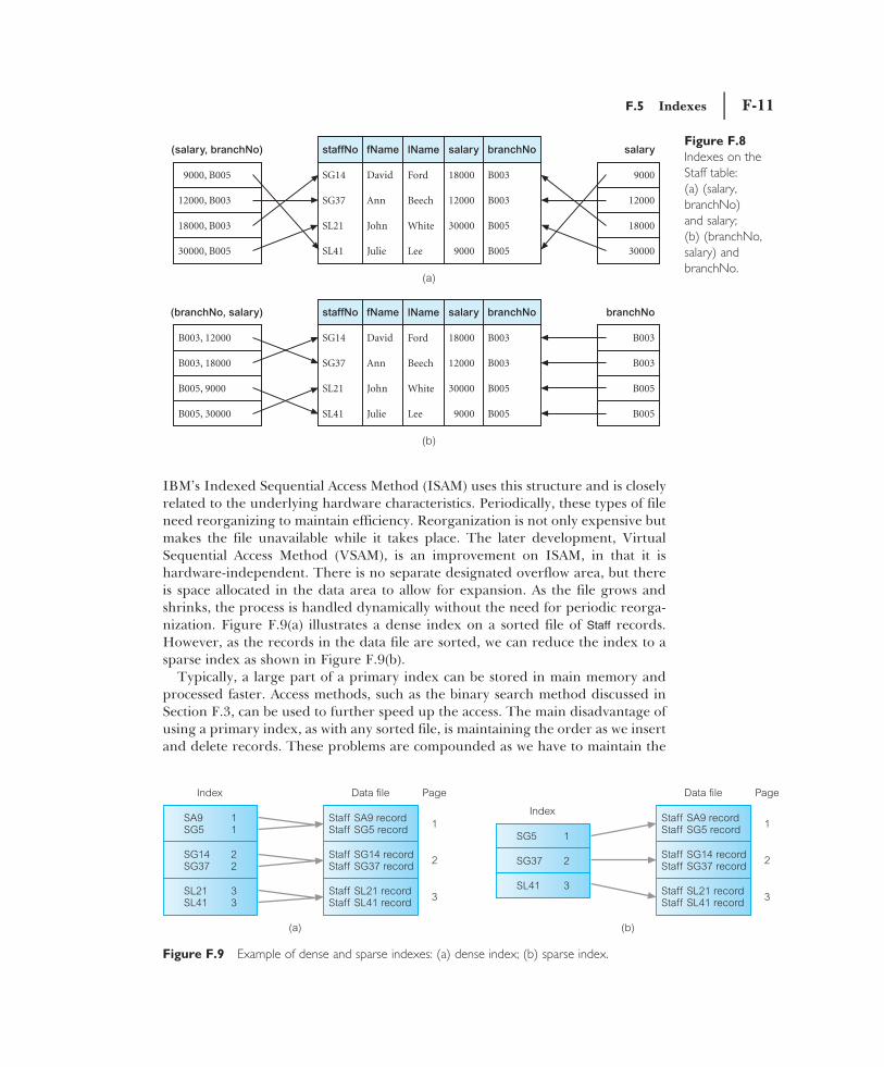
IBM’s Indexed Sequential Access Method (ISAM) uses this structure and is closelyrelated to the underlying hardware characteristics. Periodically, these types of fileneed reorganizing to maintain efficiency. Reorganization is not only expensive butmakes the file unavailable while it takes place. The later development, VirtualSequential Access Method (VSAM), is an improvement on ISAM, in that it ishardware-independent. There is no separate designated overflow area, but thereis space allocated in the data area to allow for expansion. As the file grows andshrinks, the process is handled dynamically without the need for periodic reorga-nization. Figure F.9(a) illustrates a dense index on a sorted file of Staff records.However, as the records in the data file are sorted, we can reduce the index to asparse index as shown in Figure F.9(b).

Typically, a large part of a primary index can be stored in main memory andprocessed faster. Access methods, such as the binary search method discussed inSection F.3, can be used to further speed up the access. The main disadvantage ofusing a primary index, as with any sorted file, is maintaining the order as we insertand delete records. These problems are compounded as we have to maintain the

Figure F.8

Indexes on the

Staff table:

(a) (salary,

branchNo)

and salary;

(b) (branchNo,

salary) and

branchNo.

F.5 Indexes | F-11

Figure F.9 Example of dense and sparse indexes: (a) dense index; (b) sparse index.


sorted order in the data file and in the index file. One method that can be used isthe maintenance of an overflow area and chained pointers, similar to the techniquedescribed in Section F.4 for the management of collisions in hash files.

F.5.3 Secondary IndexesA secondary index is also an ordered file similar to a primary index. However,whereas the data file associated with a primary index is sorted on the index key,the data file associated with a secondary index may not be sorted on the indexingkey. Further, the secondary index key need not contain unique values, unlike aprimary index. For example, we may wish to create a secondary index on thebranchNo column of the Staff table but from Figure F.1 we can see that the values inthe branchNo column are not unique. There are several techniques for handlingnonunique secondary indexes:

• Produce a dense secondary index that maps on to all records in the data file,thereby allowing duplicate key values to appear in the index.

• Allow the secondary index to have an index entry for each distinct key value, butallow the block pointers to be multi-valued, with an entry corresponding to eachduplicate key value in the data file.

• Allow the secondary index to have an index entry for each distinct key value.However, the block pointer would not point to the data file but to a bucket thatcontains pointers to the corresponding records in the data file.

Secondary indexes improve the performance of queries that use attributes otherthan the primary key. However, the improvement to queries has to be balancedagainst the overhead involved in maintaining the indexes while the database is beingupdated. This is part of physical database design and was discussed in Chapter 18.

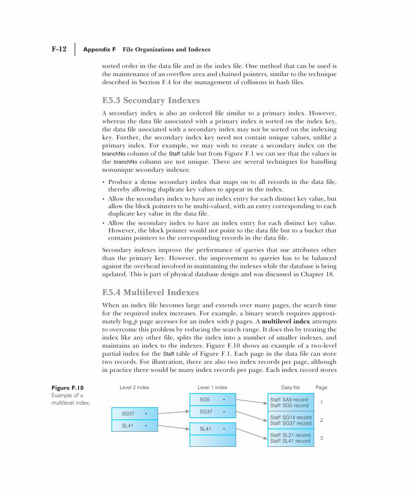
F.5.4 Multilevel IndexesWhen an index file becomes large and extends over many pages, the search timefor the required index increases. For example, a binary search requires approxi-mately log2p page accesses for an index with p pages. A multilevel index attemptsto overcome this problem by reducing the search range. It does this by treating theindex like any other file, splits the index into a number of smaller indexes, andmaintains an index to the indexes. Figure F.10 shows an example of a two-levelpartial index for the Staff table of Figure F.1. Each page in the data file can storetwo records. For illustration, there are also two index records per page, althoughin practice there would be many index records per page. Each index record stores

Figure F.10

Example of a

multilevel index.

an access key value and a page address. The stored access key value is the highestin the addressed page.

To locate a record with a specified staffNo value, say SG14, we start from the second-level index and search the page for the last access key value that is less than or equalto SG14, in this case SG37. This record contains an address to the first-level indexpage to continue the search. Repeating the process leads to page 2 in the data file,where the record is stored. If a range of staffNo values had been specified, we coulduse the same process to locate the first record in the data file corresponding to thelower range value. As the records in the data file are sorted on staffNo, we can findthe remaining records in the range by reading serially through the data file.

IBM’s ISAM is based on a two-level index structure. Insertion is handled byoverflow pages, as discussed in Section F.4. In general, an n-level index can bebuilt, although three levels are common in practice; a file would have to be verylarge to require more than three levels. In the following section we discuss a par-ticular type of multilevel dense index called a B+-tree.

F.5.5 B+-treesMany DBMSs use a data structure called a tree to hold data or indexes. A tree con-sists of a hierarchy of nodes. Each node in the tree, except the root node, has oneparent node and zero or more child nodes. A root node has no parent. A node thatdoes not have any children is called a leaf node.

The depth of a tree is the maximum number of levels between the root nodeand a leaf node in the tree. Depth may vary across different paths from root to leaf,or depth may be the same from the root node to each leaf node, producing a treecalled a balanced tree, or B-tree (Bayer and McCreight, 1972; Comer, 1979). Thedegree, or order, of a tree is the maximum number of children allowed per par-ent. Large degrees, in general, create broader, shallower trees. Because access timein a tree structure depends more often upon depth than on breadth, it is usuallyadvantageous to have “bushy,” shallow trees. A binary tree has order 2 in whicheach node has no more than two children. The rules for a B+-tree are as follows:

• If the root is not a leaf node, it must have at least two children.• For a tree of order n, each node (except the root and leaf nodes) must have between

n/2 and n pointers and children. If n/2 is not an integer, the result is rounded up.• For a tree of order n, the number of key values in a leaf node must be between

(n � 1)/2 and (n � 1) pointers and children. If (n � 1)/2 is not an integer, theresult is rounded up.

• The number of key values contained in a nonleaf node is 1 less than the num-ber of pointers.

• The tree must always be balanced: that is, every path from the root node to a leafmust have the same length.

• Leaf nodes are linked in order of key values.

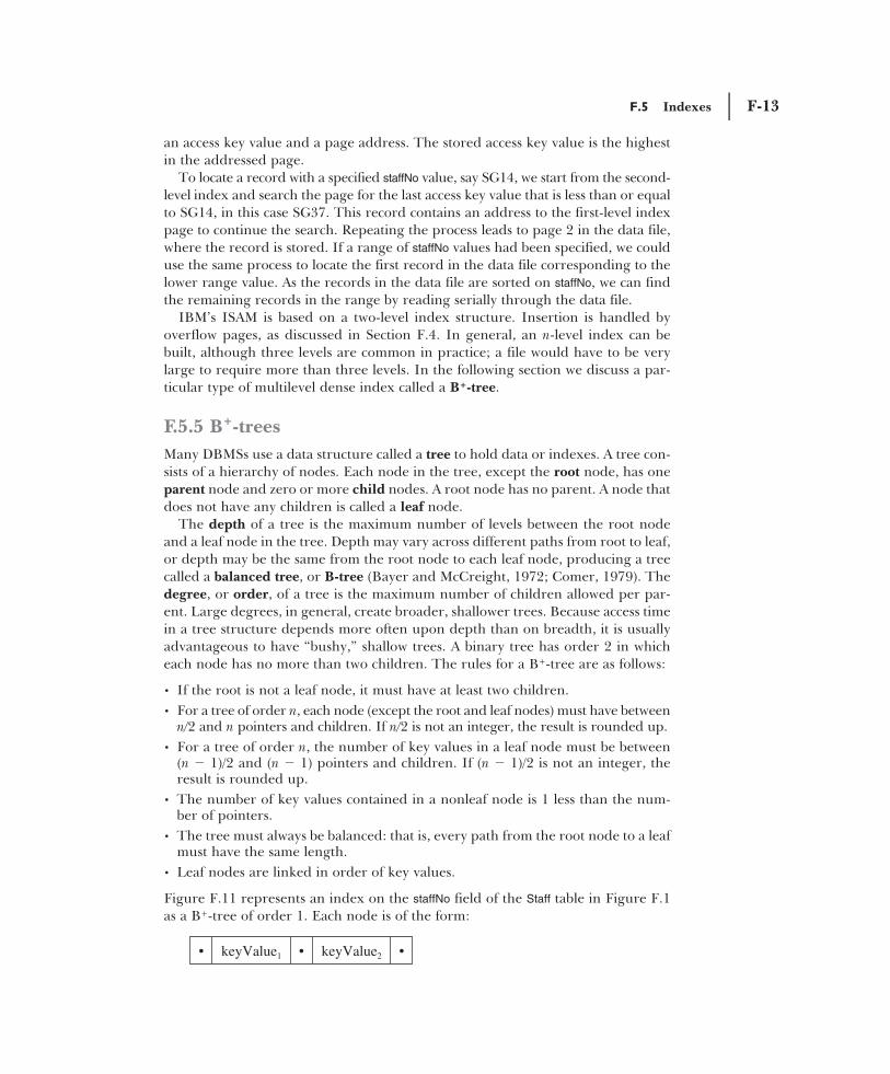
Figure F.11 represents an index on the staffNo field of the Staff table in Figure F.1as a B+-tree of order 1. Each node is of the form:

• keyValue1 • keyValue2 •

F.5 Indexes | F-13


where • can be blank or represent a pointer to another record. If the search keyvalue is less than or equal to key Valuei, the pointer to the left of key Valuei is usedto find the next node to be searched; otherwise, the pointer at the end of the nodeis used. For example, to locate SL21, we start from the root node. SL21 is greaterthan SG14, so we follow the pointer to the right, which leads to the second-levelnode containing the key values SG37 and SL21. We follow the pointer to the leftof SL21, which leads to the leaf node containing the address of record SL21.

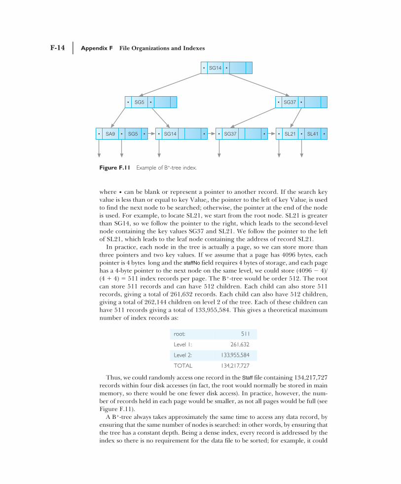
In practice, each node in the tree is actually a page, so we can store more thanthree pointers and two key values. If we assume that a page has 4096 bytes, eachpointer is 4 bytes long and the staffNo field requires 4 bytes of storage, and each pagehas a 4-byte pointer to the next node on the same level, we could store (4096 � 4)/(4 � 4) � 511 index records per page. The B+-tree would be order 512. The rootcan store 511 records and can have 512 children. Each child can also store 511records, giving a total of 261,632 records. Each child can also have 512 children,giving a total of 262,144 children on level 2 of the tree. Each of these children canhave 511 records giving a total of 133,955,584. This gives a theoretical maximumnumber of index records as:

Figure F.11 Example of B+-tree index.

root: 511

Level 1: 261,632

Level 2: 133,955,584

TOTAL 134,217,727

Thus, we could randomly access one record in the Staff file containing 134,217,727records within four disk accesses (in fact, the root would normally be stored in mainmemory, so there would be one fewer disk access). In practice, however, the num-ber of records held in each page would be smaller, as not all pages would be full (seeFigure F.11).

A B+-tree always takes approximately the same time to access any data record, byensuring that the same number of nodes is searched: in other words, by ensuring thatthe tree has a constant depth. Being a dense index, every record is addressed by theindex so there is no requirement for the data file to be sorted; for example, it could

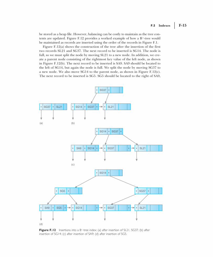
be stored as a heap file. However, balancing can be costly to maintain as the tree con-tents are updated. Figure F.12 provides a worked example of how a B+-tree wouldbe maintained as records are inserted using the order of the records in Figure F.1.

Figure F.12(a) shows the construction of the tree after the insertion of the firsttwo records SL21 and SG37. The next record to be inserted is SG14. The node isfull, so we must split the node by moving SL21 to a new node. In addition, we cre-ate a parent node consisting of the rightmost key value of the left node, as shownin Figure F.12(b). The next record to be inserted is SA9. SA9 should be located tothe left of SG14, but again the node is full. We split the node by moving SG37 toa new node. We also move SG14 to the parent node, as shown in Figure F.12(c).The next record to be inserted is SG5. SG5 should be located to the right of SA9,

F.5 Indexes | F-15

Figure F.12 Insertions into a B+-tree index: (a) after insertion of SL21, SG37; (b) after

insertion of SG14; (c) after insertion of SA9; (d) after insertion of SG5.


but again the node is full. We split the node by moving SG14 to a new node andadd SG5 to the parent node. However, the parent node is also full and has to besplit. In addition, a new parent node has to be created, as shown in Figure F.12(d).Finally, record SL41 is added to the right of SL21, as shown in Figure F.11.

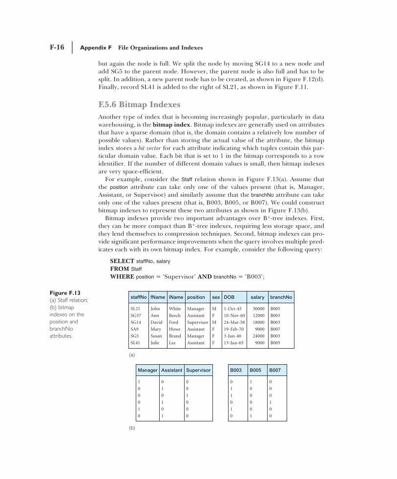
F.5.6 Bitmap IndexesAnother type of index that is becoming increasingly popular, particularly in datawarehousing, is the bitmap index. Bitmap indexes are generally used on attributesthat have a sparse domain (that is, the domain contains a relatively low number ofpossible values). Rather than storing the actual value of the attribute, the bitmapindex stores a bit vector for each attribute indicating which tuples contain this par-ticular domain value. Each bit that is set to 1 in the bitmap corresponds to a rowidentifier. If the number of different domain values is small, then bitmap indexesare very space-efficient.

For example, consider the Staff relation shown in Figure F.13(a). Assume thatthe position attribute can take only one of the values present (that is, Manager,Assistant, or Supervisor) and similarly assume that the branchNo attribute can takeonly one of the values present (that is, B003, B005, or B007). We could constructbitmap indexes to represent these two attributes as shown in Figure F.13(b).

Bitmap indexes provide two important advantages over B+-tree indexes. First,they can be more compact than B+-tree indexes, requiring less storage space, andthey lend themselves to compression techniques. Second, bitmap indexes can pro-vide significant performance improvements when the query involves multiple pred-icates each with its own bitmap index. For example, consider the following query:

SELECT staffNo, salary

FROM Staff

WHERE position = ‘Supervisor’ AND branchNo = ‘B003’;

Figure F.13

(a) Staff relation;

(b) bitmap

indexes on the

position and

branchNo

attributes.

In this case, we can take the third bit vector for position and perform a bitwise ANDwith the first bit vector for branchNo to obtain a bit vector that has a 1 for everySupervisor who works at branch ‘B003’.

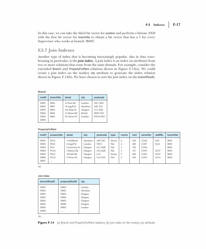
F.5.7 Join IndexesAnother type of index that is becoming increasingly popular, also in data ware-housing in particular, is the join index. A join index is an index on attributes fromtwo or more relations that come from the same domain. For example, consider theextended Branch and PropertyForRent relations shown in Figure F.14(a). We couldcreate a join index on the nonkey city attribute to generate the index relationshown in Figure F.14(b). We have chosen to sort the join index on the branchRowlD,

F.5 Indexes | F-17

Figure F.14 (a) Branch and PropertyForRent relations; (b) join index on the nonkey city attribute.


but it could have been sorted on any of the three attributes. Sometimes two joinindexes are created, one as shown and one with the two rowlD attributes reversed.

This type of query could be common in data warehousing applications whenattempting to find out facts about related pieces of data (in this case, we areattempting to find how many properties come from a city that has an existingbranch). The join index precomputes the join of the Branch and PropertyForRent rela-tions based on the city attribute, thereby removing the need to perform the joineach time the query is run, and improving the performance of the query. Thiscould be particularly important if the query has a high frequency. Oracle combinesthe bitmap index and the join index to provide a bitmap join index.

F.6 Clustered and Nonclustered Tables

Some DBMSs, such as Oracle, support clustered and nonclustered tables. Thechoice of whether to use a clustered or nonclustered table depends on the analysisof the transactions undertaken previously, but the choice can have an impact onperformance. In this section we briefly examine both types of structure.

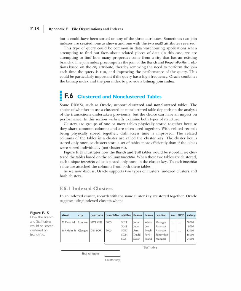
Clusters are groups of one or more tables physically stored together becausethey share common columns and are often used together. With related recordsbeing physically stored together, disk access time is improved. The relatedcolumns of the tables in a cluster are called the cluster key. The cluster key isstored only once, so clusters store a set of tables more efficiently than if the tableswere stored individually (not clustered).

Figure F.15 illustrates how the Branch and Staff tables would be stored if we clus-tered the tables based on the column branchNo. When these two tables are clustered,each unique branchNo value is stored only once, in the cluster key. To each branchNo

value are attached the columns from both these tables.As we now discuss, Oracle supports two types of clusters: indexed clusters and

hash clusters.

F.6.1 Indexed ClustersIn an indexed cluster, records with the same cluster key are stored together. Oraclesuggests using indexed clusters when:

Figure F.15

How the Branch

and Staff tables

would be stored

clustered on

branchNo.

F.6 Clustered and Nonclustered Tables | F-19

• queries retrieve records over a range of cluster key values;• clustered tables may grow unpredictably.

Clusters can improve performance of data retrieval, depending on the data dis-tribution and what SQL operations are most often performed on the data. Inparticular, tables that are joined in a query benefit from the use of clusters,because the records common to the joined tables are retrieved with the same I/Ooperation.

To create an indexed cluster in Oracle called BranchlndexedCluster with the clusterkey column branchNo, we could use the following SQL statement:

CREATE CLUSTER BranchlndexedCluster

(branchNo CHAR(4))SIZE 512STORAGE (INITIAL 100K NEXT 50K PCTINCREASE 10);

The SIZE parameter specifies the amount of space (in bytes) to store all recordswith the same cluster key value. The size is optional and, if omitted, Oraclereserves one data block for each cluster key value. The INITIAL parameter spec-ifies the size (in bytes) of the cluster’s first extent, and the NEXT parameter spec-ifies the size (in bytes) of the next extent to be allocated. The PCTINCREASEparameter specifies the percentage by which the third and subsequent extentsgrow over the preceding extent (default 50). In our example, we have specifiedthat each subsequent extent should be 10% larger than the preceding extent.

F.6.2 Hash ClustersHash clusters also cluster table data in a manner similar to index clusters.However, a record is stored in a hash cluster based on the result of applying a hashfunction to the record’s cluster key value. All records with the same hash key valueare stored together on disk. Oracle suggests using hash clusters when:

• queries retrieve records based on equality conditions involving all cluster keycolumns (for example, return all records for branch B005);

• clustered tables are static or we can determine the maximum number of recordsand the maximum amount of space required by the cluster when it is created.

To create a hash cluster in Oracle called PropertyHashCluster clustered by the columnpropertyNo, we could use the following SQL statement:

CREATE CLUSTER PropertyHashCluster

(propertyNo VARCHAR2(5))HASH IS propertyNo HASHKEYS 300000;

Once the hash cluster has been created, we can create the tables that will be partof the structure. For example:

CREATE TABLE PropertyForRent

(propertyNo VARCHAR2(5) PRIMARY KEY,...)

CLUSTER PropertyHashCluster (propertyNo);


F.7 Guidelines for Selecting File Organizations

As an aid to understanding file organizations and indexes more fully, we provideguidelines for selecting a file organization based on the following types of file:

• Heap• Hash• Indexed Sequential Access Method (ISAM)• B+-tree• Clusters

Heap (unordered)

The heap file organization is discussed in Appendix F.2. Heap is a good storagestructure in the following situations:

(1) When data is being bulk-loaded into the relation. For example, to populate arelation after it has been created, a batch of tuples may have to be inserted intothe relation. If heap is chosen as the initial file organization, it may be moreefficient to restructure the file after the insertions have been completed.

(2) The relation is only a few pages long. In this case, the time to locate any tupleis short, even if the entire relation has to be searched serially.

(3) When every tuple in the relation has to be retrieved (in any order) every time therelation is accessed. For example, retrieve the addresses of all properties for rent.

(4) When the relation has an additional access structure, such as an index key,heap storage can be used to conserve space.

Heap files are inappropriate when only selected tuples of a relation are to be accessed.

Hash

The hash file organization is discussed in Appendix F.4. Hash is a good storagestructure when tuples are retrieved based on an exact match on the hash field value,particularly if the access order is random. For example, if the PropertyForRent relationis hashed on propertyNo, retrieval of the tuple with propertyNo equal to PG36 is efficient.However, hash is not a good storage structure in the following situations:

(1) When tuples are retrieved based on a pattern match of the hash field value.For example, retrieve all properties whose property number, propertyNo, beginswith the characters “PG.”

(2) When tuples are retrieved based on a range of values for the hash field. Forexample, retrieve all properties with a rent in the range 300–500.

(3) When tuples are retrieved based on a field other than the hash field. Forexample, if the Staff relation is hashed on staffNo, then hashing cannot be usedto search for a tuple based on the IName attribute. In this case, it would be nec-essary to perform a linear search to find the tuple, or add IName as a secondaryindex (see Step 4.3).

(4) When tuples are retrieved based on only part of the hash field. For example,if the PropertyForRent relation is hashed on rooms and rent, then hashing cannot

be used to search for a tuple based on the rooms attribute alone. Again, it wouldbe necessary to perform a linear search to find the tuple.

(5) When the hash field is frequently updated. When a hash field is updated, theDBMS must delete the entire tuple and possibly relocate it to a new address (ifthe hash function results in a new address). Thus, frequent updating of thehash field affects performance.

Indexed Sequential Access Method (ISAM)

The indexed sequential file organization is discussed in Appendix F.5.2. ISAM is amore versatile storage structure than hash; it supports retrievals based on exactkey match, pattern matching, range of values, and part key specification. However,the ISAM index is static, created when the file is created. Thus, the performanceof an ISAM file deteriorates as the relation is updated. Updates also cause an ISAMfile to lose the access key sequence, so that retrievals in order of the access key willbecome slower. These two problems are overcome by the B+-tree file organization.However, unlike B+-tree, concurrent access to the index can be easily managed,because the index is static.

B+-tree

The B+-tree file organization is discussed in Appendix F.5.5. Again, B+-tree is amore versatile storage structure than hashing. It supports retrievals based onexact key match, pattern matching, range of values, and part key specification.The B+-tree index is dynamic, growing as the relation grows. Thus, unlikeISAM, the performance of a B+-tree file does not deteriorate as the relation isupdated. The B+-tree also maintains the order of the access key even when thefile is updated, so retrieval of tuples in the order of the access key is more effi-cient than ISAM. However, if the relation is not frequently updated, the ISAMstructure may be more efficient, as it has one fewer level of index than the B+-tree, whose leaf nodes contain pointers to the actual tuples rather than thetuples themselves.

Clustered tables

Some DBMSs, for example Oracle, support clustered tables (see Appendix F.6).The choice of whether to use a clustered or nonclustered table depends on theanalysis of the transactions undertaken previously, but the choice can have animpact on performance. Following, we provide guidelines for the use of clusteredtables. Note in this section, we use the Oracle terminology, which refers to a rela-tion as a table with columns and rows.

Clusters are groups of one or more tables physically stored together becausethey share common columns and are often used together. With related rows beingphysically stored together, disk access time is improved. The related columns ofthe tables in a cluster are called the cluster key. The cluster key is stored only once,so clusters store a set of tables more efficiently than if the tables were stored indi-vidually (not clustered). Oracle supports two types of clusters: indexed clusters andhash clusters.

F.7 Guidelines for Selecting File Organizations | F-21


(a) Indexed clusters In an indexed cluster, rows with the same cluster key arestored together. Oracle suggests using indexed clusters when:

• queries retrieve rows over a range of cluster key values;• clustered tables may grow unpredictably.

The following guidelines may be helpful when deciding whether to cluster tables:

• Consider clustering tables that are often accessed in join statements.• Do not cluster tables if they are joined only occasionally or their common col-

umn values are modified frequently. (Modifying a row’s cluster key value takeslonger than modifying the value in an unclustered table, because Oracle mayhave to migrate the modified row to another block to maintain the cluster.)

• Do not cluster tables if a full search of one of the tables is often required. (Afull search of a clustered table can take longer than a full search of an unclus-tered table. Oracle is likely to read more blocks, because the tables are storedtogether.)

• Consider clustering tables involved in a one-to-many (1:*) relationship if a rowis often selected from the parent table and then the corresponding rows from thechild table. (Child rows are stored in the same data block(s) as the parent row,so they are likely to be in memory when selected, requiring Oracle to performless I/O.)

• Consider storing a child table alone in a cluster if many child rows are selectedfrom the same parent. (This measure improves the performance of queries thatselect child rows of the same parent but does not decrease the performance of afull search of the parent table.)

• Do not cluster tables if the data from all tables with the same cluster key valueexceeds more than one or two Oracle blocks. (To access a row in a clusteredtable, Oracle reads all blocks containing rows with that value. If these rowsoccupy multiple blocks, accessing a single row could require more reads thanaccessing the same row in an unclustered table.)

(b) Hash clusters Hash clusters also cluster table data in a manner similar toindex clusters. However, a row is stored in a hash cluster based on the result ofapplying a hash function to the row’s cluster key value. All rows with the same hashkey value are stored together on disk. Oracle suggests using hash clusters when:

• queries retrieve rows based on equality conditions involving all cluster keycolumns (for example, return all rows for branch B003);

• clustered tables are static or the maximum number of rows and the maximumamount of space required by the cluster can be determined when it is created.

The following guidelines may be helpful when deciding whether to use hash clusters:

• Consider using hash clusters to store tables that are frequently accessed using asearch clause containing equality conditions with the same column(s). Designatethese column(s) as the cluster key.

• Store a table in a hash cluster if it can be determined how much space is requiredto hold all rows with a given cluster key value, both now and in the future.

• Do not use hash clusters if space is scarce and it is not affordable to allocate addi-tional space for rows to be inserted in the future.

Appendix Summary | F-23

• Do not use a hash cluster to store a constantly growing table if the process ofoccasionally creating a new, larger hash cluster to hold that table is impractical.

• Do not store a table in a hash cluster if a search of the entire table is oftenrequired and a significant amount of space must be allocated to the hash clusterin anticipation of the table growing. (Such full searches must read all blocks allo-cated to the hash cluster, even though some blocks may contain few rows.Storing the table alone would reduce the number of blocks read by a full tablesearch.)

• Do not store a table in a hash cluster if the cluster key values are frequentlymodified.

• Storing a single table in a hash cluster can be useful, regardless of whether thetable is often joined with other tables, provided that hashing is appropriate forthe table based on the previous guidelines.

Appendix Summary

• A file organization is the physical arrangement of data in a file into records and pages of secondary storage.

An access method is the steps involved in storing and retrieving records from a file.

• Heap (unordered) files store records in the same order they are inserted. Heap files are good for inserting a

large number of records into the file. They are inappropriate when only selected records are to be retrieved.

• Sequential (ordered) files store records sorted on the values of one or more fields (the ordering fields).

Inserting and deleting records in a sorted file is problematic, because the order of records has to be maintained.

As a result, ordered files are rarely used for database storage unless a primary index is added to the file.

• Hash files are good when retrieval is based on an exact key match. They are not good when retrieval is based

on pattern matching, range of values, part keys, or a column other than the hash field.

• An index is a data structure that allows the DBMS to locate particular records in a file more quickly and thereby

speed response to user queries. There are three main types of index: a primary index, clustering index, and

a secondary index (an index that is defined on a non-ordering field of the data file).

• Secondary indexes provide a mechanism for specifying an additional key for a base relation that can be used

to retrieve data more efficiently. However, there is an overhead involved in the maintenance and use of sec-

ondary indexes that has to be balanced against the performance improvement gained when retrieving data.

• ISAM is more versatile than hashing, supporting retrievals based on exact key match, pattern matching, range of

values, and part key specification. However, the ISAM index is static, so performance deteriorates as the table is

updated. Updates also cause the ISAM file to lose the access key sequence, so retrievals in order of the access

key become slower.

• These two problems are overcome by the B+-tree file organization, which has a dynamic index. However, unlike

B+-tree, because the ISAM index is static, concurrent access to the index can be easily managed. If the relation is

not frequently updated or not very large or likely to be, the ISAM structure may be more efficient as it has one

less level of index than the B+-tree, whose leaf nodes contain record pointers.

• A bitmap index stores a bit vector for each attribute indicating which tuples contain this particular domain

value. Each bit that is set to 1 in the bitmap corresponds to a row identifier. If the number of different domain

values is small, then bitmap indexes are very space efficient.


• A join index is an index on attributes from two or more relations that come from the same domain. The join

index precomputes the join of the two relations based on the specified attribute, thereby removing the need to

perform the join each time the query is run, and improving the performance of the query. This could be par-

ticularly important if the query has a high frequency.

• Clusters are groups of one or more tables physically stored together because they share common columns

and are often used together. With related records being physically stored together, disk access time is improved.

The related columns of the tables in a cluster are called the cluster key. The cluster key is stored only once,

and so clusters store a set of tables more efficiently than if the tables were stored individually (not clustered).

Oracle supports two types of clusters: indexed clusters and hash clusters.

Documents

Appendix F: File Organizations and Indexeswps.aw.com/wps/media/objects/7095/7265991/appendices/AppendixF… · Chapter 18 require the selection of appropriate file organizations and