Appli Cs

7/24/2019 Appli Cs

http://slidepdf.com/reader/full/appli-cs 1/5

MSM1Aa MATHS CORE A: APPLICATIONS OF

DIFFERENTIATION

1. L’Hopital’s Rule for Limits

Fact 1.1. Suppose that x1 < a < x2, that f an g are differentiable on (x1, x2) andthat g(a) = 0. Suppose also that

(1) limx→a

f (x) = limx→a

g(x) = 0 and

(2) limx→a f

(x)g(x) exists.

Then

limx→a

f (x)

g(x) = lim

x→a

f (x)

g(x).

2. Increasing and Decreasing Functions

Definition 2.1. Let f be a real-valued function f of a real variable and let I = (x1, x2)be an interval in dom(f ). Then f is said to be:

(1) increasing (non-decreasing) on I if f (a) ≤ f (b) whenever a, b ∈ I and a < b;(2) strictly increasing on I if f (a) < f (b) whenever a, b ∈ I and a < b;(3) decreasing (non-increasing) on I if f (a) ≥ f (b) whenever a, b ∈ I and a < b;(4) strictly decreasing on I if f (a) > f (b) whenever a, b ∈ I and a < b.

Fact 2.2. Let f be a real-valued function of a real variable that is differentiable onI = (x1, x2).

(1) f (x) ≥ 0 for all x ∈ I if and only if f is non-decreasing on I .(2) If f (x) > 0 for all x ∈ I , then f is strictly increasing on I .(3) f (x) ≤ 0 for all x ∈ I if and only if f is non-increasing on I .

(4) If f

(x) < 0 for all x ∈ I , then f is strictly decreasing on I .

1

7/24/2019 Appli Cs


2 MSM1AA MATHS CORE A: APPLICATIONS OF DIFFERENTIATION

3. Concave Functions and Points of Inflexion

Definition 3.1. Let f be a real-valued function of a real variable that is differentiableon I = (x1, x2).

(1) (The graph of) f is concave up on I if f (x) strictly increasing on I .(2) (The graph of) f is concave down on I if f (x) strictly decreasing on I .(3) A point c ∈ I is a point of inflexion of f if:

(a) either, f is concave up on (x1, c) and concave down on (c, x2);(b) or, f is concave down on (x1, c) and concave up on (c, x2).

From Fact 2.2 we have the following:

Fact 3.2. Let f be a real-valued function of a real variable that is twice differentiableon I = (x1, x2).

(1) If f (x) > 0 for all x ∈ (x1, x2), then f is concave up on (x1, x2).(2) If f (x) < 0 for all x ∈ (x1, x2), then f is concave down on (x1, x2).(3) If c ∈ (x1, x2) is a point of inflexion, then f (c) = 0.(4) If f (c) = 0 and f changes sign at c, then c is a point of inflexion.

Note that if c is a point if inflexion, then f (c) does not have to be 0. To findpoints of inflexion, first identify all points c such that f (c) = 0 and then determineat which of these points f changes sign.

4. Stationary Points and Extrema

Definition 4.1. Let f be a real-valued function of a real variable.

(1) f has a local maximum at c if there is some open interval (x1, x2) containingc such that f (x) f (c) for all x ∈ (x1, x2).

(2) f has a absolute or global maximum at c if f (x) f (c) for all x ∈ dom(f ).(3) f has a local minimum at c if there is some open interval (x1, x2) containing

c such that f (x) f (c) for all x ∈ (x1, x2).(4) f has a absolute or global minimum at c if f (x) f (c) for all x ∈ dom(f ).(5) f has a local (or global) extremum at c if it has either a local (or global)

maximum or minimum at c.

Definition 4.2. Let f be a real-valued function of a real variable. The point c is astationary point of f if f (c) = 0.

Stationary points are often called turning or critical points.

Fact 4.3. Let f : [x1, x2] → R be a continuous function. Then f has a globalmaximum and a global minimum (we say that f attains its bounds). Moreover, eachglobal extremum of f is either:

(1) an end point of the interval [x1, x2]; or(2) a point where the derivative of f does not exist; or(3) a stationary point of f .

7/24/2019 Appli Cs


MSM1Aa MATHS CORE A: APPLICATIONS OF DIFFERENTIATION 3

5. Classifying Stationary Points

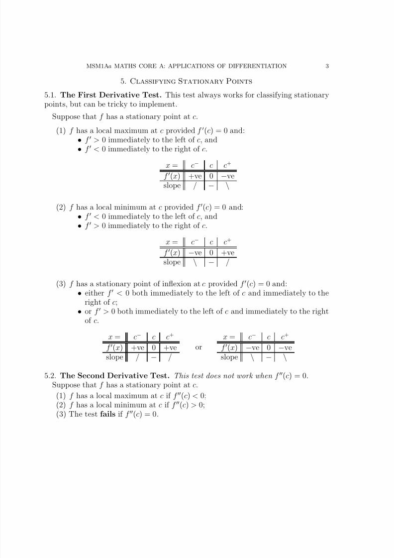
5.1. The First Derivative Test. This test always works for classifying stationarypoints, but can be tricky to implement.

Suppose that f has a stationary point at c.

(1) f has a local maximum at c provided f (c) = 0 and:• f > 0 immediately to the left of c, and• f < 0 immediately to the right of c.

x = c− c c+

f (x) +ve 0 −veslope / − \

(2) f has a local minimum at c provided f (c) = 0 and:• f < 0 immediately to the left of c, and• f > 0 immediately to the right of c.

x = c− c c+

f (x) −ve 0 +veslope \ − /

(3) f has a stationary point of inflexion at c provided f (c) = 0 and:

• either f

< 0 both immediately to the left of c and immediately to theright of c;

• or f > 0 both immediately to the left of c and immediately to the rightof c.

x = c− c c+

f (x) +ve 0 +veslope / − /

or

x = c− c c+

f (x) −ve 0 −veslope \ − \

5.2. The Second Derivative Test. This test does not work when f (c) = 0.Suppose that f has a stationary point at c.

(1) f has a local maximum at c if f (c) < 0;(2) f has a local minimum at c if f (c) > 0;(3) The test fails if f (c) = 0.

7/24/2019 Appli Cs


4 MSM1AA MATHS CORE A: APPLICATIONS OF DIFFERENTIATION

6. Graph Sketching

(1) Use your knowledge of functions.(2) Identify the asymptotic behaviour of y = f (x) as x → ±∞. If y = f (x)approaches a line y = mx + c, then this line is an oblique asymptote. It isalso possible for y = f (x) to be asymptotic to other functions. Try to identifywhether y = f (x) lies above the asymptote or below it. In particular, if f (x) → c as x → ±∞, then there is a horizontal asymptote.

(3) Identify the asymptotic behaviour of y = f (x) near points where y tends to±∞: if f (x) → ±∞ as x → c, what happens at c+ and c−, i.e. just to theright of c and just to the left? It is possible for f to tend to +∞ on one sideof c and −∞ on the other, or for it to tend to +∞ on both sides of c, or −∞on both sides. These are the vertical asymptotes of y = f (x).

(4) Plot easy to calculate key points (x- and y-intercepts, stationary points).(5) Observe whether y is positive or negative in key regions, greater than or

smaller than an asymptote.(6) Calculate f : find and classify the stationary points (if any) and note where

the gradient is positive or negative.(7) Calculate f : find any points of inflexion and note where the function is

concave up and concave down.

7. Tangents, Normals and Inverse Functions

Definition 7.1. Let f : R → R be a function and (a, b) be a point on the graph of f

(so that b = f (a)). The tangent to the graph of f at (a, b) is the straight line passingthrough the point (a, b) which has the same gradient as f at (a, b). The normal tothe graph of f at (a, b) is the straight line passing through (a, b) perpendicular to thetangent at (a, b).

Fact 7.2. The gradient of f at (a, b) is f (a), hence the gradient of the tangent tothe graph at the point (a, b) is f (a).

The gradient of the normal to the graph at (a, b) is −1/f (a).

The equation of the tangent to the graph of f at (a, b) is given by f (a) = y − b

x − a.

The equation of the normal to the graph of f at (a, b) is given by −1

f (a) =

y − b

x−

a,

provided f (a) = 0. If f (a) = 0, then the normal has equation x = a.These equations can be rearranged into the standard form y = cx + d.

The Graph of an Inverse Function

Suppose that f : R → R is a function with an inverse f −1. Then the graph of f is the set of points in R

2 of the form (x, y) where y = f (x) and the graph of f −1 isthe set of points in R

2 of the form (y, x) where x = f −1(y) (note that it does notmatter what letter we use to represent the dependent and independent variables).Now y = f (x) if and only if x = f −1(y) and (x, y) the reflection of (y, x) in the liney = x. Hence the graph of f −1 is the reflection of the graph of f in the line y = x.

7/24/2019 Appli Cs


MSM1Aa MATHS CORE A: APPLICATIONS OF DIFFERENTIATION 5

8. Examples

Example. Determine limx→0(cos x − 1)/x2

.Solution. As x → 0, both cos x − 1 → 0 and x2 → 0, so by l’Hopital’s Rule

limx→0

cos x − 1

x2 = lim

x→0

− sin x

2x .

Again, as x → 0, both − sin x → 0 and 2x → 0, so we can apply l’Hopital’s Rule asecond time to get

limx→0

cos x − 1

x2 = lim

x→0

− sin x

2x = lim

x→0

− cos x

2 = −1

2.

Example. Although f (0) = 0, f (x) = x4 does not have a point of inflexion at 0.

Example. Let f (x) = x3 + 2x2− x − 2, find the regions where f is strictly increasingand strictly decreasing and find the points of inflexion of f .

Solution. f (x) = x3 + 2x2 − x − 2 = (x − 1)(x + 1)(x + 2), f (x) = 3x2 + 4x − 1 andf (x) = 6x + 4. The roots of 3x2 + 4x − 1 are (−2 ± √

7)/3, so f is strictly positive,and hence f is strictly increasing on

−∞, (−2 −√ 7)/3

and on

(−2 +

√ 7)/3, ∞

.

f is strictly negative, so f is strictly decreasing on

(−2 − √ 7)/3, (−2 +

√ 7)/3

.

For the points of inflexion f (x) = 0, when x = −2/3. So x = −2/3 is a possiblepoint of inflexion. If x is lightly less than −2/3, 6x is slightly less than −4, sof (x) < 0. If x is slightly greater than −2/3, then 6x is slightly greater than −4, sothat f (x) > 0. Hence f changes sign at

−2/3, so this is a point of inflexion.

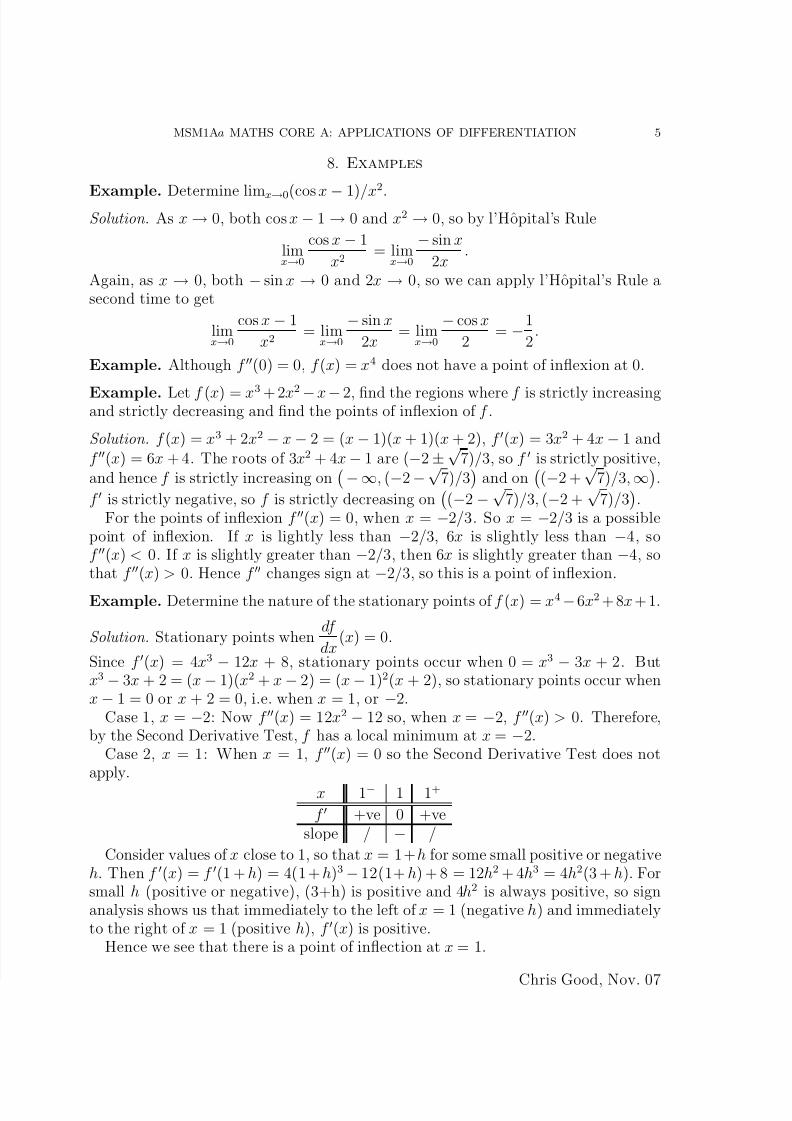
Example. Determine the nature of the stationary points of f (x) = x4−6x2 + 8x + 1.

Solution. Stationary points when df

dx(x) = 0.

Since f (x) = 4x3 − 12x + 8, stationary points occur when 0 = x3 − 3x + 2. Butx3 − 3x + 2 = (x − 1)(x2 + x − 2) = (x − 1)2(x + 2), so stationary points occur whenx − 1 = 0 or x + 2 = 0, i.e. when x = 1, or −2.

Case 1, x = −2: Now f (x) = 12x2 − 12 so, when x = −2, f (x) > 0. Therefore,by the Second Derivative Test, f has a local minimum at x = −2.

Case 2, x = 1: When x = 1, f (x) = 0 so the Second Derivative Test does notapply.

x 1− 1 1+

f +ve 0 +veslope / − /

Consider values of x close to 1, so that x = 1+h for some small positive or negativeh. Then f (x) = f (1 + h) = 4(1 + h)3 − 12(1+ h) + 8 = 12h2 + 4h3 = 4h2(3 + h). Forsmall h (positive or negative), (3+h) is positive and 4h2 is always positive, so signanalysis shows us that immediately to the left of x = 1 (negative h) and immediatelyto the right of x = 1 (positive h), f (x) is positive.

Hence we see that there is a point of inflection at x = 1.

Chris Good, Nov. 07

Documents

Appli Cs