Chapter 4

Application Products of NWP

4.1 Summary

The results of NWP are indispensable elements to weather forecasting both for general public and for specialpurposes, and therefore JMA disseminates them in real time to the local offices of JMA, private companies, andrelated organizations both in Japan and abroad. Although facsimile charts have been the primary means of dis-tributing NWP output for a long time, at the present time dissemination in the form of Grid Point Values (GPV)is the essential method with the progress of telecommunication infrastructure and sophisticated visualizationsystems.

In addition to the raw NWP data, value-added products derived from NWP output are also disseminated.One example of such products is information on parameters not explicitly calculated in NWP models, suchas probabilistic forecasts and turbulence potential for aviation. Another is error-reduced estimation of NWPoutput parameters, with statistics of the relationship between NWP output and the corresponding observation.JMA has been disseminating Very-short-range (6 hour) Forecast of Precipitation and the Hourly Analysis ofhorizontal wind and temperature field, a three-dimensional variational (3D-Var) method is utilized for HourlyAnalysis. To support middle to long-range forecasting, JMA has been disseminating various kind of forecastcharts and Grid Point Value for one-week forecast and one-month and seasonal forecast.

In the following sections, specification of Application Products of NWP and their utilization in the JMAoffices are demonstrated.

4.2 Weather Chart Services

Facsimile chart is a conventional service to disseminate the result of NWP in a graphical form. The JMA’sfacsimile charts are sent to national meteorological services via the Global Telecommunication System (GTS)and to ships via the shortwave radio transmission (call sign JMH).

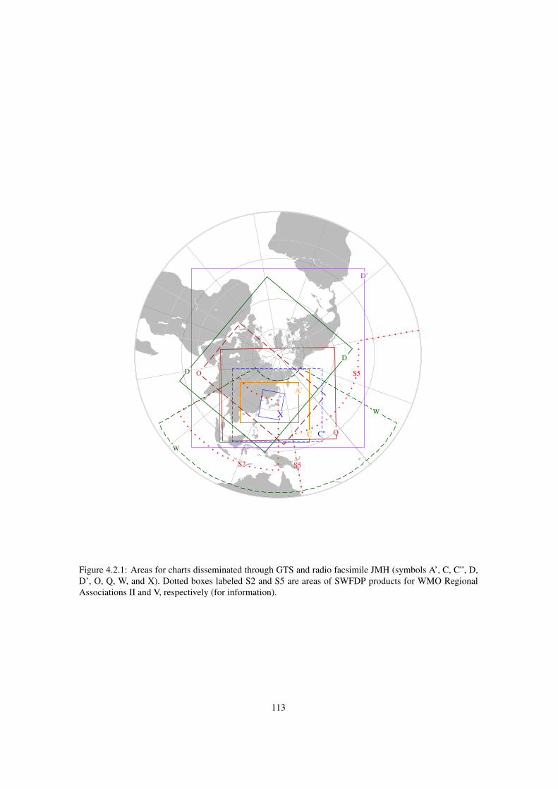
Table 4.2.1 and Figure 4.2.1 give summaries of weather charts easily accessible for international users,namely charts served through GTS and JMH.

The Web is emerging alternative to complement and innovate above services. A number of projects arerunning worldwide. JMA takes part in international projects such as Project on the Provision of City-SpecificNumerical Weather Prediction (NWP) Products to Developing Countries via the Internet in the WMO RegionalAssociation II (RA II) or the Severe Weather Forecast Demonstration Project (SWFDP) in WMO RAs II andV. There are also JMA’s own projects, such as JMA Pilot Project on EPS Products or SATAID Services on theWMO Information System.

111

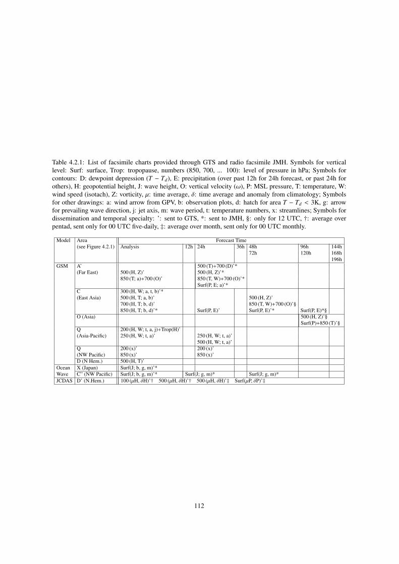
Table 4.2.1: List of facsimile charts provided through GTS and radio facsimile JMH. Symbols for verticallevel: Surf: surface, Trop: tropopause, numbers (850, 700, ... 100): level of pressure in hPa; Symbols forcontours: D: dewpoint depression (T − Td), E: precipitation (over past 12h for 24h forecast, or past 24h forothers), H: geopotential height, J: wave height, O: vertical velocity (ω), P: MSL pressure, T: temperature, W:wind speed (isotach), Z: vorticity, µ: time average, δ: time average and anomaly from climatology; Symbolsfor other drawings: a: wind arrow from GPV, b: observation plots, d: hatch for area T − Td < 3K, g: arrowfor prevailing wave direction, j: jet axis, m: wave period, t: temperature numbers, x: streamlines; Symbols fordissemination and temporal specialty: ’: sent to GTS, *: sent to JMH, §: only for 12 UTC, †: average overpentad, sent only for 00 UTC five-daily, ‡: average over month, sent only for 00 UTC monthly.

Model Area Forecast Time(see Figure 4.2.1) Analysis 12h 24h 36h 48h 96h 144h

72h 120h 168h196h

GSM A’ 500 (T)+700 (D)’*(Far East) 500 (H, Z)’ 500 (H, Z)’*

850 (T; a)+700 (O)’ 850 (T, W)+700 (O)’*Surf(P, E; a)’*

C 300 (H, W; a, t, b)’*(East Asia) 500 (H, T; a, b)’ 500 (H, Z)’

700 (H, T; b, d)’ 850 (T, W)+700 (O)’§850 (H, T; b, d)’* Surf(P, E)’ Surf(P, E)’* Surf(P, E)*§

O (Asia) 500 (H, Z)’§Surf(P)+850 (T)’§

Q 200 (H, W; t, a, j)+Trop(H)’(Asia-Pacific) 250 (H, W; t, a)’ 250 (H, W; t, a)’

500 (H, W; t, a)’Q 200 (x)’ 200 (x)’(NW Pacific) 850 (x)’ 850 (x)’D (N Hem.) 500 (H, T)’

Ocean X (Japan) Surf(J; b, g, m)’*Wave C” (NW Pacific) Surf(J; b, g, m)’* Surf(J; g, m)* Surf(J; g, m)*JCDAS D’ (N.Hem.) 100 (µH, δH)’† 500 (µH, δH)’† 500 (µH, δH)’‡ Surf(µP, δP)’‡

112

A’

C

O

Q

W

W

D

D

C"

D’

X

S2 S5

S5

Figure 4.2.1: Areas for charts disseminated through GTS and radio facsimile JMH (symbols A’, C, C”, D,D’, O, Q, W, and X). Dotted boxes labeled S2 and S5 are areas of SWFDP products for WMO RegionalAssociations II and V, respectively (for information).

113

4.3 GPV ProductsAs a part of JMA’s general responsibility of meteorological information service, the grid point values (GPV)products are distributed to domestic and international users. In conformance to requirement of the WMOInformation System (WIS), this data service utilizes both dedicated and public (i.e. the Internet) networkinfrastructure.

The dedicated infrastructure consists of an international part called GTS, together with domestic partsinside JMA (including the Meteorological Satellite Center and the Meteorological Research Institute) andtoward government agencies and Meteorological Business Support Center, which is in charge of managedservice for general users including the private sector.

The portal to JMA’s international services over the Internet is the website of Global Information SystemCentre (GISC) Tokyo 1. The WMO Distributed Data Bases (DDBs) and RSMC Data Serving System (RSMCDSS) are integrated into GISC Tokyo. Currently the international service of GPV products includes GSM,One-week EPS, and Ocean Wave Model, as listed in Table 4.3.1.

4.4 Very-short-range Forecasting of PrecipitationJMA has been routinely operating a fully automated system for semi-hourly analysis and very-short-rangeforecasting of precipitation since 1988 to provide products for monitoring and forecasting local severe weather.The products are :

1. Analysis of precipitation called the “Radar-Raingauge Analyzed Precipitation” (hereafter R/A) basedon the radar observations operated by JMA and the other organization and the raingauge measurementsoperated by JMA(the Automated Meteorological Data Acquisition System, hereafter AMeDAS) and theother organizations,

2. Semi-hourly forecasts of 1-hour accumulated precipitation called the “Very-Short-Range-Forecasting ofPrecipitation” (hereafter VSRF) based on extrapolation and forecast by the Meso-scale Model (MSM,see Section 3.5). The forecast time of VSRF is from 1 to 6 hour.

The spatial resolution of these products are 1km. These products are made available in about 20 minutesafter observation time every half hour. They are transmitted to local meteorological observatories, and the localgovernments and broadcasting stations which are responsible for disaster prevention.

4.4.1 Analysis of Precipitation (R/A)R/A uses data of 46 radars (JMA 20, the other organization 26) and up to about 10, 000 raingauges (AMeDAS1, 300, the other organizations 8, 700). These data are combined to benefit from advantages of both facili-ties: the advantage of the radar is its high resolution in space and that of raingauge is its high accuracy ofprecipitation measurement.

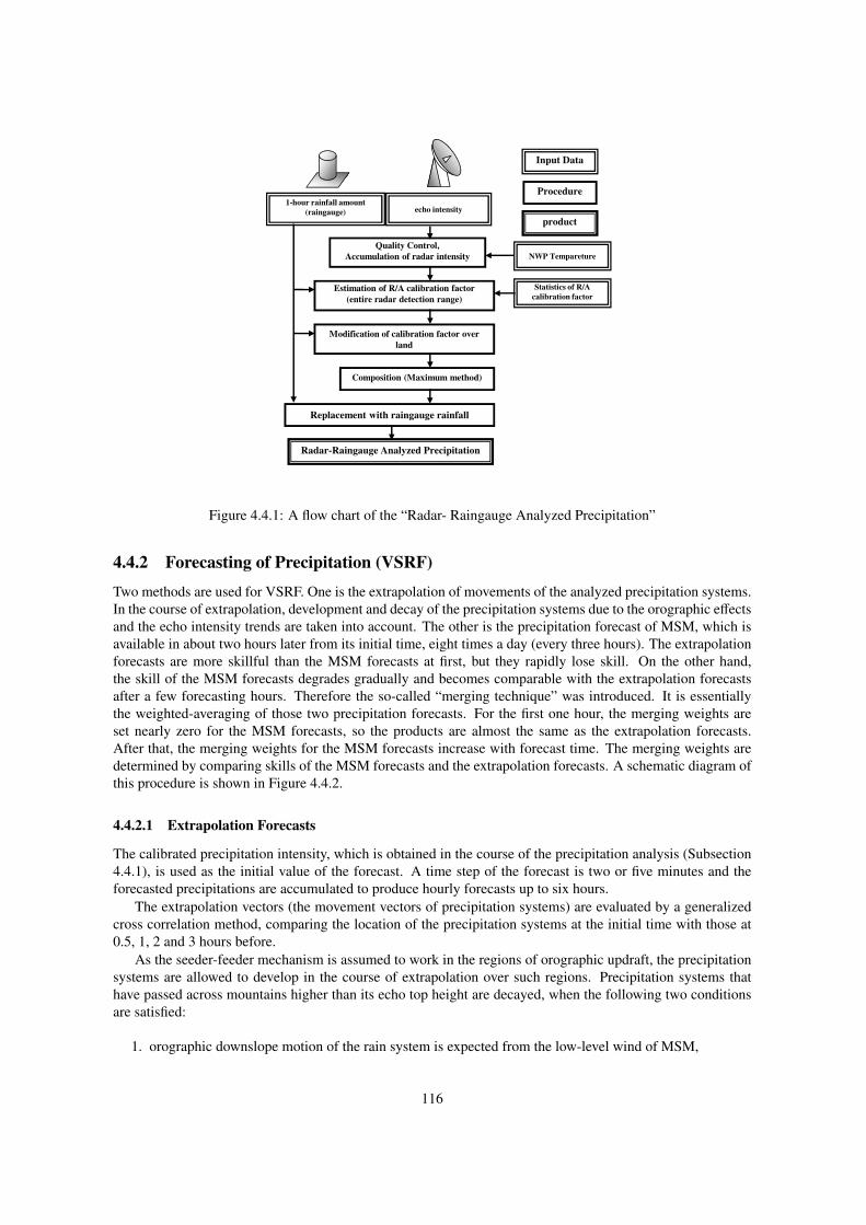
The one-hour accumulated precipitation amounts estimated using radar observation are usually differentfrom those observed with raingauges. The radar precipitation amounts are calibrated into more accurate pre-cipitation using the raingauge precipitation data (Makihara 2000). First, calibration factors over the entiredetection range of each radar are calculated by comparing the radar precipitation of the multiple radars andraingauge data. When comparing radar precipitation, the difference of radar beam height is taken into account.Then the estimated calibration factor is further modified using raingauge data to estimate local heavy precip-itation more accurately at each grid which contains raingauges. For the grid has no raingauges, the modifiedcalibration factors is calculated with weighted interpolation of the calibration factors of the surrounding gridsthat contain raingauges. Composition of all radar’s calibrated precipitation into a nationwide chart is madeby the maximum value method, in which the largest value is selected if a grid has several data observed bymultiple radars. A schematic diagram of this procedure is shown in Figure 4.4.1.

1http://www.wis-jma.go.jp

114

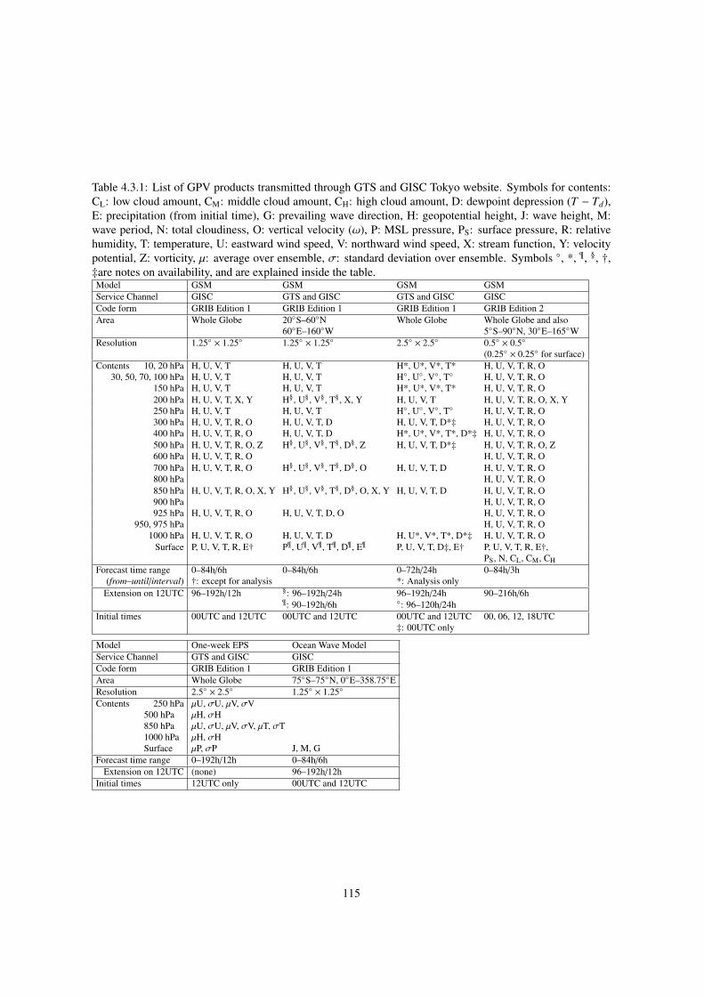
Table 4.3.1: List of GPV products transmitted through GTS and GISC Tokyo website. Symbols for contents:CL: low cloud amount, CM: middle cloud amount, CH: high cloud amount, D: dewpoint depression (T − Td),E: precipitation (from initial time), G: prevailing wave direction, H: geopotential height, J: wave height, M:wave period, N: total cloudiness, O: vertical velocity (ω), P: MSL pressure, PS: surface pressure, R: relativehumidity, T: temperature, U: eastward wind speed, V: northward wind speed, X: stream function, Y: velocitypotential, Z: vorticity, µ: average over ensemble, σ: standard deviation over ensemble. Symbols , *, ¶, §, †,‡are notes on availability, and are explained inside the table.Model GSM GSM GSM GSMService Channel GISC GTS and GISC GTS and GISC GISCCode form GRIB Edition 1 GRIB Edition 1 GRIB Edition 1 GRIB Edition 2Area Whole Globe 20S–60N Whole Globe Whole Globe and also

60E–160W 5S–90N, 30E–165WResolution 1.25 × 1.25 1.25 × 1.25 2.5 × 2.5 0.5 × 0.5

(0.25 × 0.25 for surface)Contents 10, 20 hPa H, U, V, T H, U, V, T H*, U*, V*, T* H, U, V, T, R, O

30, 50, 70, 100 hPa H, U, V, T H, U, V, T H, U, V, T H, U, V, T, R, O150 hPa H, U, V, T H, U, V, T H*, U*, V*, T* H, U, V, T, R, O200 hPa H, U, V, T, X, Y H§, U§, V§, T§, X, Y H, U, V, T H, U, V, T, R, O, X, Y250 hPa H, U, V, T H, U, V, T H, U, V, T H, U, V, T, R, O300 hPa H, U, V, T, R, O H, U, V, T, D H, U, V, T, D*‡ H, U, V, T, R, O400 hPa H, U, V, T, R, O H, U, V, T, D H*, U*, V*, T*, D*‡ H, U, V, T, R, O500 hPa H, U, V, T, R, O, Z H§, U§, V§, T§, D§, Z H, U, V, T, D*‡ H, U, V, T, R, O, Z600 hPa H, U, V, T, R, O H, U, V, T, R, O700 hPa H, U, V, T, R, O H§, U§, V§, T§, D§, O H, U, V, T, D H, U, V, T, R, O800 hPa H, U, V, T, R, O850 hPa H, U, V, T, R, O, X, Y H§, U§, V§, T§, D§, O, X, Y H, U, V, T, D H, U, V, T, R, O900 hPa H, U, V, T, R, O925 hPa H, U, V, T, R, O H, U, V, T, D, O H, U, V, T, R, O

950, 975 hPa H, U, V, T, R, O1000 hPa H, U, V, T, R, O H, U, V, T, D H, U*, V*, T*, D*‡ H, U, V, T, R, O

Surface P, U, V, T, R, E† P¶, U¶, V¶, T¶, D¶, E¶ P, U, V, T, D‡, E† P, U, V, T, R, E†,PS, N, CL, CM, CH

Forecast time range 0–84h/6h 0–84h/6h 0–72h/24h 0–84h/3h(from–until/interval) †: except for analysis *: Analysis only

Extension on 12UTC 96–192h/12h §: 96–192h/24h 96–192h/24h 90–216h/6h¶: 90–192h/6h : 96–120h/24h

Initial times 00UTC and 12UTC 00UTC and 12UTC 00UTC and 12UTC 00, 06, 12, 18UTC‡: 00UTC only

Model One-week EPS Ocean Wave ModelService Channel GTS and GISC GISCCode form GRIB Edition 1 GRIB Edition 1Area Whole Globe 75S–75N, 0E–358.75EResolution 2.5 × 2.5 1.25 × 1.25

Contents 250 hPa µU, σU, µV, σV500 hPa µH, σH850 hPa µU, σU, µV, σV, µT, σT1000 hPa µH, σHSurface µP, σP J, M, G

Forecast time range 0–192h/12h 0–84h/6hExtension on 12UTC (none) 96–192h/12h

Initial times 12UTC only 00UTC and 12UTC

115

Statistics of R/A

calibration factor

1-hour rainfall amount

(raingauge) echo intensity

Quality Control,

Accumulation of radar intensity

Estimation of R/A calibration factor

(entire radar detection range)

Modification of calibration factor over

land

Composition (Maximum method)

Input Data

Procedure

product

NWP Tempareture

Replacement with raingauge rainfall

Radar-Raingauge Analyzed Precipitation

Figure 4.4.1: A flow chart of the “Radar- Raingauge Analyzed Precipitation”

4.4.2 Forecasting of Precipitation (VSRF)

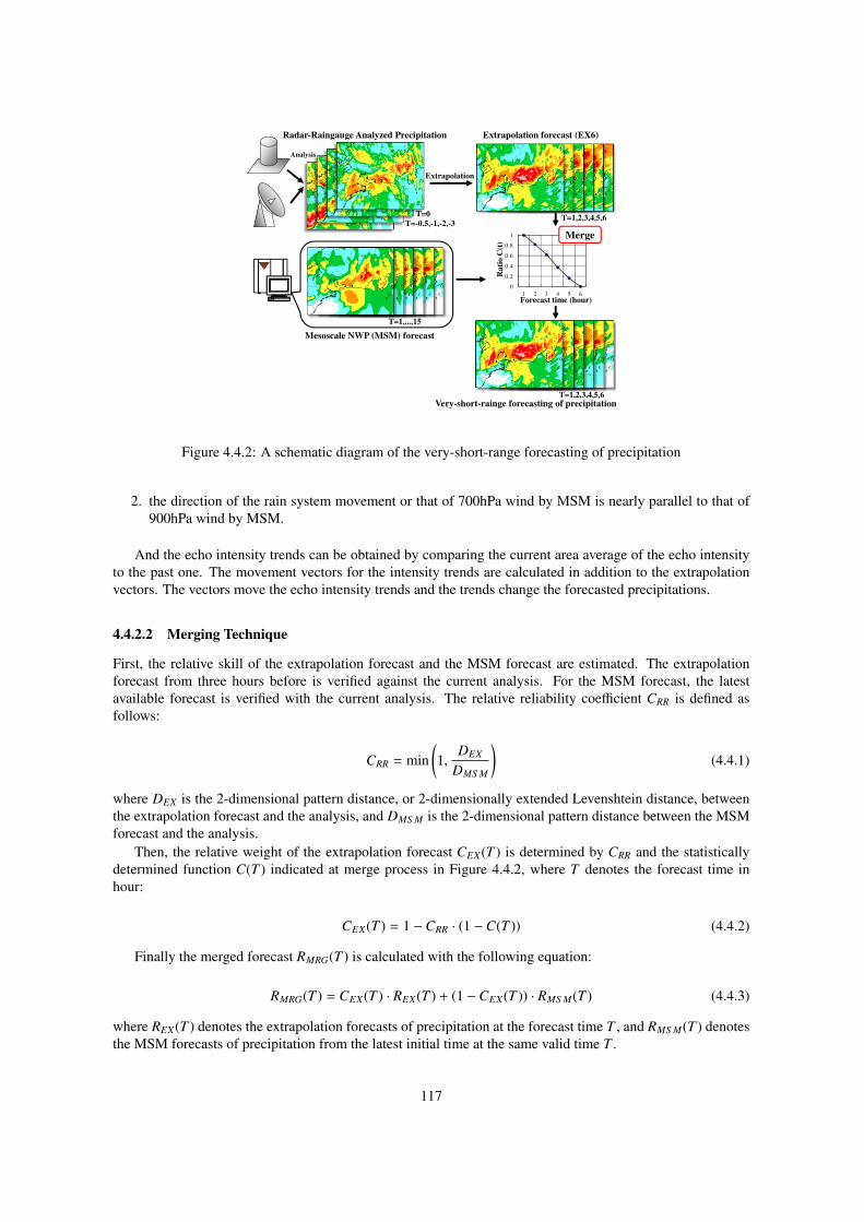
Two methods are used for VSRF. One is the extrapolation of movements of the analyzed precipitation systems.In the course of extrapolation, development and decay of the precipitation systems due to the orographic effectsand the echo intensity trends are taken into account. The other is the precipitation forecast of MSM, which isavailable in about two hours later from its initial time, eight times a day (every three hours). The extrapolationforecasts are more skillful than the MSM forecasts at first, but they rapidly lose skill. On the other hand,the skill of the MSM forecasts degrades gradually and becomes comparable with the extrapolation forecastsafter a few forecasting hours. Therefore the so-called “merging technique” was introduced. It is essentiallythe weighted-averaging of those two precipitation forecasts. For the first one hour, the merging weights areset nearly zero for the MSM forecasts, so the products are almost the same as the extrapolation forecasts.After that, the merging weights for the MSM forecasts increase with forecast time. The merging weights aredetermined by comparing skills of the MSM forecasts and the extrapolation forecasts. A schematic diagram ofthis procedure is shown in Figure 4.4.2.

4.4.2.1 Extrapolation Forecasts

The calibrated precipitation intensity, which is obtained in the course of the precipitation analysis (Subsection4.4.1), is used as the initial value of the forecast. A time step of the forecast is two or five minutes and theforecasted precipitations are accumulated to produce hourly forecasts up to six hours.

The extrapolation vectors (the movement vectors of precipitation systems) are evaluated by a generalizedcross correlation method, comparing the location of the precipitation systems at the initial time with those at0.5, 1, 2 and 3 hours before.

As the seeder-feeder mechanism is assumed to work in the regions of orographic updraft, the precipitationsystems are allowed to develop in the course of extrapolation over such regions. Precipitation systems thathave passed across mountains higher than its echo top height are decayed, when the following two conditionsare satisfied:

1. orographic downslope motion of the rain system is expected from the low-level wind of MSM,

116

0.2

0.4

0.6

0.8

1

Radar-Raingauge Analyzed Precipitation

Analysis

Extrapolation

T=0

T=-0.5,-1,-2,-3

Extrapolation forecast (EX6)

T=1,2,3,4,5,6

Ra

tio

C(t

)

Merge

0

1 2 3 4 5 6

T=1,...,15

Mesoscale NWP (MSM) forecast

Forecast time (hour)

T=1,2,3,4,5,6Very-short-rainge forecasting of precipitation

Figure 4.4.2: A schematic diagram of the very-short-range forecasting of precipitation

2. the direction of the rain system movement or that of 700hPa wind by MSM is nearly parallel to that of900hPa wind by MSM.

And the echo intensity trends can be obtained by comparing the current area average of the echo intensityto the past one. The movement vectors for the intensity trends are calculated in addition to the extrapolationvectors. The vectors move the echo intensity trends and the trends change the forecasted precipitations.

4.4.2.2 Merging Technique

First, the relative skill of the extrapolation forecast and the MSM forecast are estimated. The extrapolationforecast from three hours before is verified against the current analysis. For the MSM forecast, the latestavailable forecast is verified with the current analysis. The relative reliability coefficient CRR is defined asfollows:

CRR = min(1,

DEX

DMS M

)(4.4.1)

where DEX is the 2-dimensional pattern distance, or 2-dimensionally extended Levenshtein distance, betweenthe extrapolation forecast and the analysis, and DMS M is the 2-dimensional pattern distance between the MSMforecast and the analysis.

Then, the relative weight of the extrapolation forecast CEX(T ) is determined by CRR and the statisticallydetermined function C(T ) indicated at merge process in Figure 4.4.2, where T denotes the forecast time inhour:

CEX(T ) = 1 −CRR · (1 −C(T )) (4.4.2)

Finally the merged forecast RMRG(T ) is calculated with the following equation:

RMRG(T ) = CEX(T ) · REX(T ) + (1 −CEX(T )) · RMS M(T ) (4.4.3)

where REX(T ) denotes the extrapolation forecasts of precipitation at the forecast time T , and RMS M(T ) denotesthe MSM forecasts of precipitation from the latest initial time at the same valid time T .

117

4.4.3 Example and Verification ScoreAn example of the R/A and VSRF is shown in Figure 4.4.3. The R/A in the Kyushu region, southwestern areaof Japan at 20UTC 23 June 2012 is shown in the left panel (a), and the 3-hour forecast of VSRF at the samevalid time, i.e. its initial time is at 17UTC 23 June 2012, is shown in the right panel (b). The intense rain bandis well forecasted.

(a) ANAL(R/A) (b) VSRF

1 5 10 20 [mm/h]

Figure 4.4.3: An example of (a) the Radar-Raingauge Analyzed Precipitation at 20UTC 23 June 2012 and (b)the 3-hour forecast of precipitation of VSRF at the same valid time

The accuracy of VSRF has been statistically verified with the Critical Success Index (CSI)2. Forecasts arecompared with precipitation analysis after both fields are averaged in 20km× 20km grids. The threshold valueis set as 1mm/hr. Indices from 1-hour to 6-hour forecasts for June 2012 are shown in Figure 4.4.4, togetherwith those of the extrapolation, MSM, and the persistence forecasts.

It can be seen that the scores get worse as forecast time gets longer. Up to three hours, the extrapolationforecast keeps its superiority to MSM, but the relationship of them becomes reverse after four hours, whileVSRF behaves best performance through all forecast times.

4.5 Hourly AnalysisThe hourly analysis provides grid point value data of three-dimensional temperature and wind analysis everyhour, assisting forecasters in monitoring the atmosphere. Imagery products are also available to users in theaviation sector through a meteorological information web page.

The configuration of the hourly analysis system is listed in Table 4.5.1. The hourly analysis uses an objec-tive analysis scheme of a 3-dimensional variational (3D-Var) method, which is implemented as a part of the“JMA Nonhydrostatic model”-based Variational Analysis Data Assimilation (JNoVA; Honda et al. 2005). Theanalysis uses the latest Meso-scale Model (MSM, Section 3.5) forecast as the first guess (a 2-4 hour forecastdepending on the analysis time). The domain of the hourly analysis is the same as that of the MSM (MA) (Fig-ure 2.6.2), covering Japan and its surrounding area (3,600 km by 2,880 km) at the same horizontal resolutionas that in the MSM (with a grid spacing of 5 km). The hourly analysis has fifty vertical layers defined in thez*-coordinate, with the top of the domain at 21,801 m.

2The CSI is the number of correct “yes” forecasts divided by the total number of occasions on which that event was forecast and/orobserved. It is also cited as “Threat Score”.

118

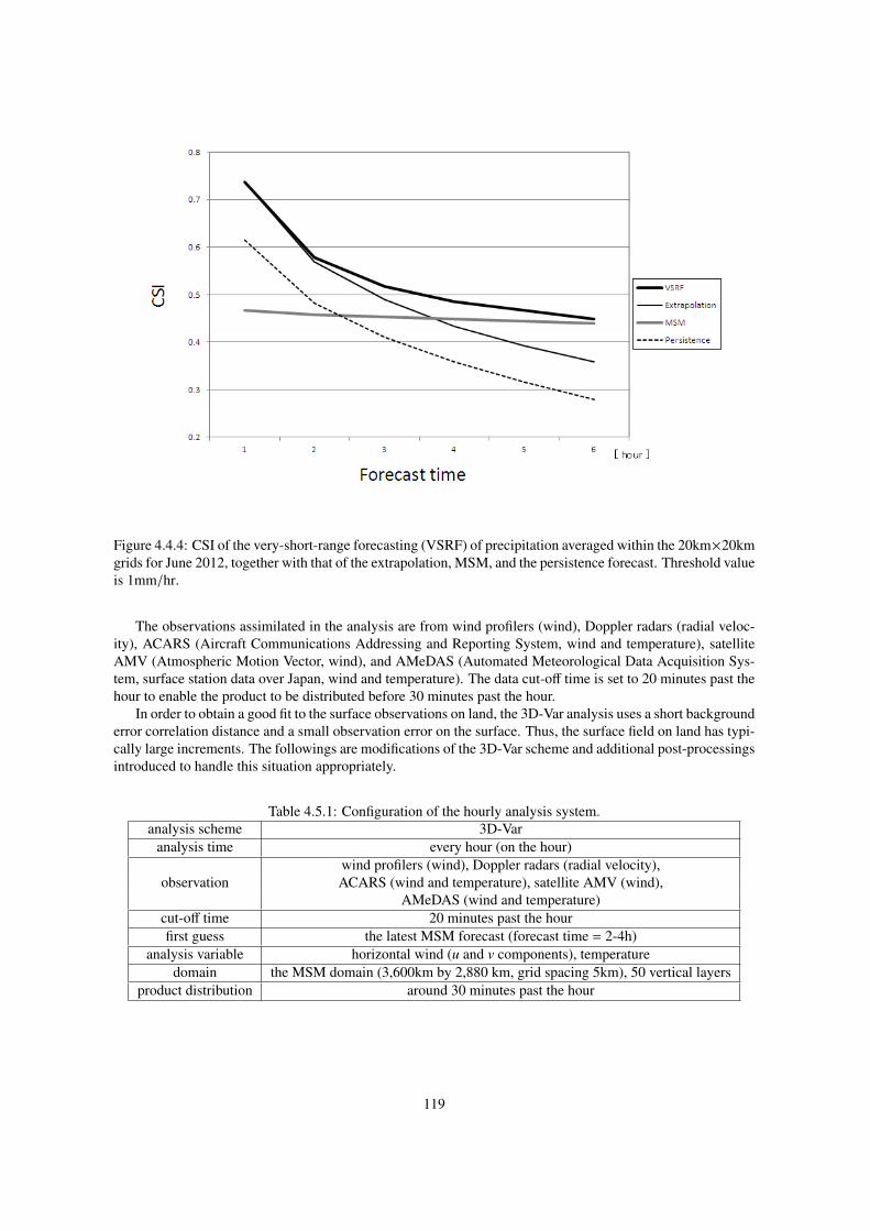
Figure 4.4.4: CSI of the very-short-range forecasting (VSRF) of precipitation averaged within the 20km×20kmgrids for June 2012, together with that of the extrapolation, MSM, and the persistence forecast. Threshold valueis 1mm/hr.

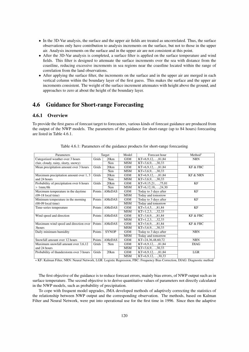
The observations assimilated in the analysis are from wind profilers (wind), Doppler radars (radial veloc-ity), ACARS (Aircraft Communications Addressing and Reporting System, wind and temperature), satelliteAMV (Atmospheric Motion Vector, wind), and AMeDAS (Automated Meteorological Data Acquisition Sys-tem, surface station data over Japan, wind and temperature). The data cut-off time is set to 20 minutes past thehour to enable the product to be distributed before 30 minutes past the hour.

In order to obtain a good fit to the surface observations on land, the 3D-Var analysis uses a short backgrounderror correlation distance and a small observation error on the surface. Thus, the surface field on land has typi-cally large increments. The followings are modifications of the 3D-Var scheme and additional post-processingsintroduced to handle this situation appropriately.

Table 4.5.1: Configuration of the hourly analysis system.analysis scheme 3D-Var

analysis time every hour (on the hour)wind profilers (wind), Doppler radars (radial velocity),

observation ACARS (wind and temperature), satellite AMV (wind),AMeDAS (wind and temperature)

cut-off time 20 minutes past the hourfirst guess the latest MSM forecast (forecast time = 2-4h)

analysis variable horizontal wind (u and v components), temperaturedomain the MSM domain (3,600km by 2,880 km, grid spacing 5km), 50 vertical layers

product distribution around 30 minutes past the hour

119

• In the 3D-Var analysis, the surface and the upper air fields are treated as uncorrelated. Thus, the surfaceobservations only have contribution to analysis increments on the surface, but not to those in the upperair. Analysis increments on the surface and in the upper air are not consistent at this point.• After the 3D-Var analysis is completed, a surface filter is applied on the surface temperature and wind

fields. This filter is designed to attenuate the surface increments over the sea with distance from thecoastline, reducing excessive increments in sea regions near the coastline located within the range ofcorrelation from the land observations.• After applying the surface filter, the increments on the surface and in the upper air are merged in each

vertical column within the boundary layer of the first guess. This makes the surface and the upper airincrements consistent. The weight of the surface increment attenuates with height above the ground, andapproaches to zero at about the height of the boundary layer.

4.6 Guidance for Short-range Forecasting

4.6.1 OverviewTo provide the first guess of forecast target to forecasters, various kinds of forecast guidance are produced fromthe output of the NWP models. The parameters of the guidance for short-range (up to 84 hours) forecastingare listed in Table 4.6.1.

Table 4.6.1: Parameters of the guidance products for short-range forecasting

Parameters Target Model Forecast hour Method∗

Categorized weather over 3 hours Grids 20km GSM KT=6,9,12,. . .,81,84 NRN(fair, cloudy, rainy, sleety, snowy) 5km MSM KT=3,6,9,. . .,30,33Mean precipitation amount over 3 hours Grids 20km GSM KT=6,9,12,. . .,81,84 KF & FBC

5km MSM KT=3,6,9,. . .,30,33Maximum precipitation amount over 1, 3 Grids 20km GSM KT=6,9,12,. . .,81,84 KF & NRNand 24 hours 5km MSM KT=3,6,9,. . .,30,33Probability of precipitation over 6 hours Grids 20km GSM KT=9,15,21,. . .,75,81 KF> 1mm/6h 5km MSM KT=6,12,18,. . .,24,30Maximum temperature in the daytime Points AMeDAS GSM Today to 3 days after KF(09-18 local time) MSM Today and tomorrowMinimum temperature in the morning Points AMeDAS GSM Today to 3 days after KF(00-09 local time) MSM Today and tomorrowTime-series temperature Points AMeDAS GSM KT=3,4,5,. . .,81,84 KF

MSM KT=1,2,3,. . .,32,33Wind speed and direction Points AMeDAS GSM KT=3,6,9,. . .,81,84 KF & FBC

MSM KT=1,2,3,. . .,32,33Maximum wind speed and direction over Points AMeDAS GSM KT=3,6,9,. . .,81,84 KF & FBC3hours MSM KT=3,6,9,. . .,30,33Daily minimum humidity Points SYNOP GSM Today to 3 days after NRN

MSM Today and tomorrowSnowfall amount over 12 hours Points AMeDAS GSM KT=24,36,48,60,72 NRNMaximum snowfall amount over 3,6,12 Grids 5km GSM KT=6,9,12,. . .,81,84 DIAGand 24 hours MSM KT=3,6,9,. . .,30,33Probability of thunderstorm over 3 hours Grids 20km GSM KT=6,9,12,. . .,81,84 LGR

MSM KT=6,9,12,. . .,30,33∗ KF: Kalman Filter, NRN: Neural Network, LGR: Logistic Regression, FBC: Frequency Bias Correction, DIAG: Diagnostic method

The first objective of the guidance is to reduce forecast errors, mainly bias errors, of NWP output such as insurface temperature. The second objective is to derive quantitative values of parameters not directly calculatedin the NWP models, such as probability of precipitation.

To cope with frequent model upgrades, JMA developed methods of adaptively correcting the statistics ofthe relationship between NWP output and the corresponding observation. The methods, based on KalmanFilter and Neural Network, were put into operational use for the first time in 1996. Since then the adaptive

120

methods have been applied to most of the parameters, replacing the formerly used non-adaptive multivariateregression method.

In the following subsections, Kalman Filter and Neural Network used in the guidance system are explainedin Subsection 4.6.2 and Subsection 4.6.3, respectively, and the utilization of the guidance in forecasting officesis summarized in Subsection 4.6.4.

4.6.2 Guidance by Kalman Filter4.6.2.1 Kalman Filter

As a statistical post-processing method of NWP output, Kalman Filter (KF) was developed in JMA on the basisof earlier works of Persson (1991) and Simonsen (1991). The notation of KF, which basically follows that ofPersson (1991), is as follows:

y: predictand (target of forecast)

ccc: predictors (1 × n matrix)

XXX: coefficients (n × 1 matrix)

QQQ: covariance of XXX (n × n matrix)

τ: sequence number of NWP initial times

First, the observation equation, which is a linear model for relating the predictand with the pre-selectedpredictors, and the system equations are given as:

yτ = cccτXXXτ + vτ (4.6.1)XXXτ+1 = AAAτXXXτ + uuuτ (4.6.2)

where vτ is the observational random error whose variance is Dτ, and uuuτ is the random error vector of thesystem, whose covariance matrix is UUUτ. The matrix AAAτ describes the evolution of the coefficients in time andis set to the unit matrix in this case;

AAAτ ≡ III (4.6.3)

The objective of KF is to obtain the most likely estimation of the coefficients XXXτ+1/τ, whose subscriptsdenote that this is an estimate using the observation corresponding to the forecast at τ and used for the predictionat τ + 1. In contrast, single subscripts in Eq. (4.6.1) and Eq. (4.6.2) denote the “true” values at τ. XXXτ+1/τ isobtained from the previous estimate XXXτ/τ−1 and the forecast error:

XXXτ+1/τ = XXXτ/τ (4.6.4)= XXXτ/τ−1 + δτ(yτ − cccτXXXτ/τ−1) (4.6.5)

where

δτ = QQQτ/τ−1cccTτ (cccτQQQτ/τ−1cccT

τ + Dτ)−1 (4.6.6)

QQQ, the covariance of XXX, is updated as follows:

QQQτ+1/τ = QQQτ/τ +UUUτ (4.6.7)= QQQτ/τ−1 − δτcccτQQQτ/τ−1 +UUUτ (4.6.8)

Eq. (4.6.4) and Eq. (4.6.7) are derived from Eq. (4.6.2) and Eq. (4.6.3).Finally, the forecast value is calculated with the updated coefficients and predictors at τ + 1;

121

yτ+1/τ = cccτ+1XXXτ+1/τ (4.6.9)

For some forecast parameters, temperature for example, the predictand y is the difference between the NWPoutput and the observation, while for the others, precipitation amount for example, y is the observation itself.

In the forecast guidance system with KF, Dτ in Eq. (4.6.6) and UUUτ in Eq. (4.6.8) are treated as empiricalparameters of controlling the adaptation speed.

4.6.2.2 Frequency Bias Correction

With KF, the most likely estimation of the predictand which minimizes the expected root-mean-square erroris obtained. However, the output has a tendency of lower frequency of forecasting rare events, such as strongwind and heavy rain, than the actual. To compensate this unfavorable feature, a frequency bias correctionscheme is applied to the KF output of some parameters.

The basic idea is to multiply the estimation of KF, y, by a correction factor F(y) to get the final output yb:

yb = y · F(y)

To determine F(y), a number of thresholds ti are chosen to span the given observation data set first. Thencorresponding thresholds f i for the forecast data set are adjusted so that the number of observation data smallerthan ti should approximate to that of forecast data smaller than f i. Finally the correction factors are computedas follows:

F( f i) = ti/ f i

F(y) for f i < y < f i+1 is linearly interpolated between F( f i) and F( f i+1).

Since KF is an adaptive method, f i is also updated each time the observation yτ corresponding to the estimatesof KF yτ/τ−1 is available. The update procedure is as follows:

f iτ+1 =

f iτ(1 + α) if yτ < ti and yτ/τ−1 > f i

f iτ(1 − α) if yτ > ti and yτ/τ−1 < f i

f iτ otherwise

where α is an empirical parameter to determine the adaptation speed. This frequency bias correction is appliedto the guidance for wind and precipitation amount.

4.6.2.3 An Example of the Guidance by Kalman Filter (3-hour Precipitation Amount)

In this guidance, the predictand is the observed 3-hour accumulated precipitation amount averaged within a20km × 20km square, and the following nine parameters derived from GSM forecast are used as predictors.

1. NW85: NW − SE component of wind speed at 850hPa

2. NE85: NE − SW component of wind speed at 850hPa

3. SSI: Showalter’s stability index

4. OGES: Orographic precipitation index

5. PCWV: Precipitable water contents × wind speed at 850hPa × ascending speed at 850hPa

6. QWX: Σ (Specific humidity × ascending speed × relative humidity) between 1000 and 300hPa

7. EHQ: Σ (Depth of wet layer × specific humidity) between 1000 and 300hPa

8. DXQV: Precipitation index on winter synoptic pattern

122

9. FRR: Precipitation by the model (GSM)

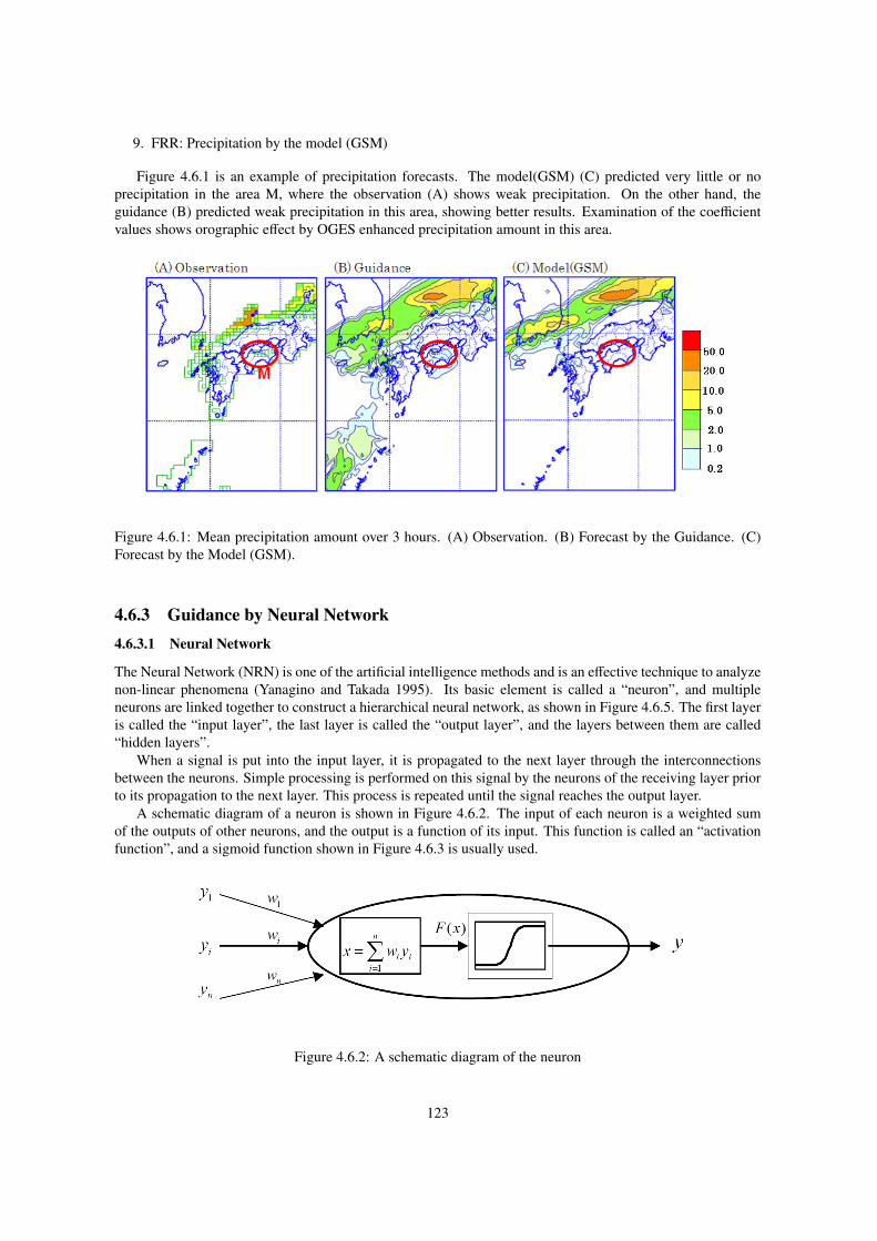
Figure 4.6.1 is an example of precipitation forecasts. The model(GSM) (C) predicted very little or noprecipitation in the area M, where the observation (A) shows weak precipitation. On the other hand, theguidance (B) predicted weak precipitation in this area, showing better results. Examination of the coefficientvalues shows orographic effect by OGES enhanced precipitation amount in this area.

Figure 4.6.1: Mean precipitation amount over 3 hours. (A) Observation. (B) Forecast by the Guidance. (C)Forecast by the Model (GSM).

4.6.3 Guidance by Neural Network4.6.3.1 Neural Network

The Neural Network (NRN) is one of the artificial intelligence methods and is an effective technique to analyzenon-linear phenomena (Yanagino and Takada 1995). Its basic element is called a “neuron”, and multipleneurons are linked together to construct a hierarchical neural network, as shown in Figure 4.6.5. The first layeris called the “input layer”, the last layer is called the “output layer”, and the layers between them are called“hidden layers”.

When a signal is put into the input layer, it is propagated to the next layer through the interconnectionsbetween the neurons. Simple processing is performed on this signal by the neurons of the receiving layer priorto its propagation to the next layer. This process is repeated until the signal reaches the output layer.

A schematic diagram of a neuron is shown in Figure 4.6.2. The input of each neuron is a weighted sumof the outputs of other neurons, and the output is a function of its input. This function is called an “activationfunction”, and a sigmoid function shown in Figure 4.6.3 is usually used.

Figure 4.6.2: A schematic diagram of the neuron

123

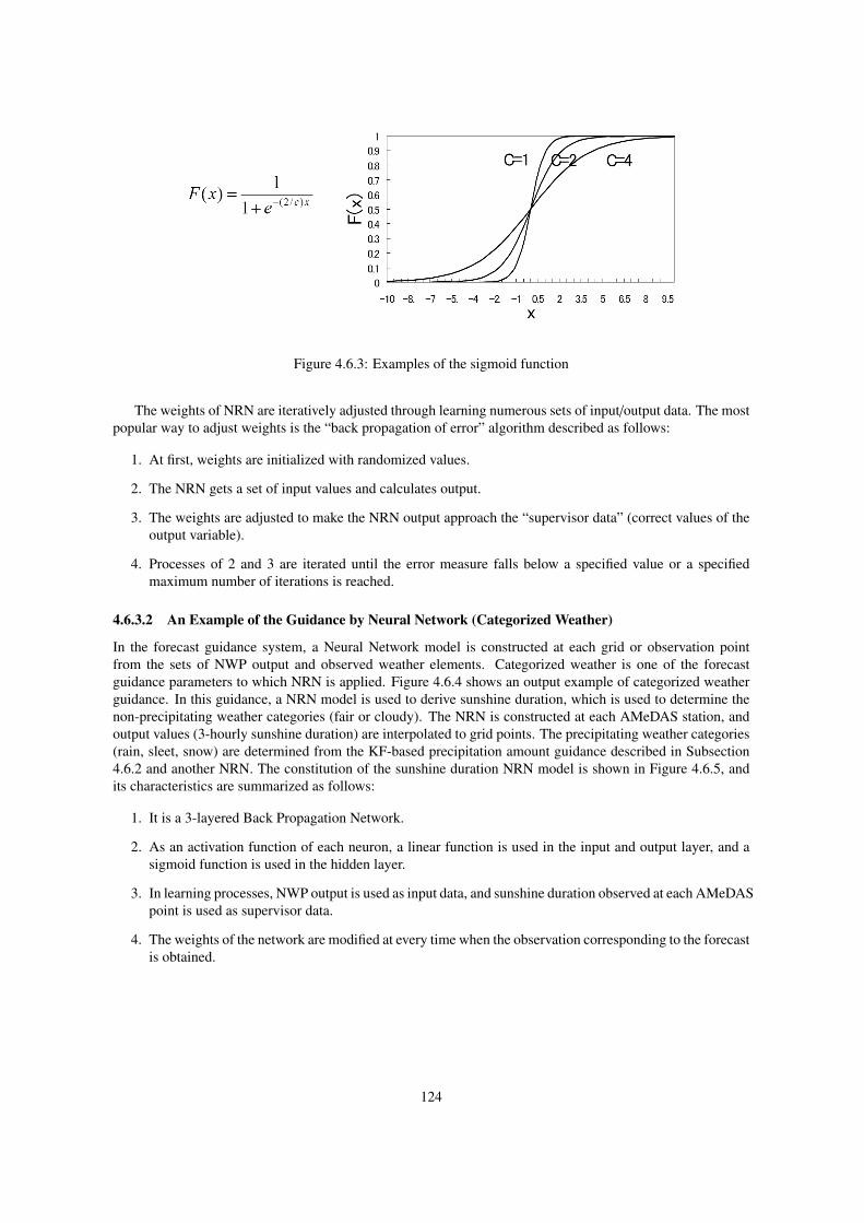
Figure 4.6.3: Examples of the sigmoid function

The weights of NRN are iteratively adjusted through learning numerous sets of input/output data. The mostpopular way to adjust weights is the “back propagation of error” algorithm described as follows:

1. At first, weights are initialized with randomized values.

2. The NRN gets a set of input values and calculates output.

3. The weights are adjusted to make the NRN output approach the “supervisor data” (correct values of theoutput variable).

4. Processes of 2 and 3 are iterated until the error measure falls below a specified value or a specifiedmaximum number of iterations is reached.

4.6.3.2 An Example of the Guidance by Neural Network (Categorized Weather)

In the forecast guidance system, a Neural Network model is constructed at each grid or observation pointfrom the sets of NWP output and observed weather elements. Categorized weather is one of the forecastguidance parameters to which NRN is applied. Figure 4.6.4 shows an output example of categorized weatherguidance. In this guidance, a NRN model is used to derive sunshine duration, which is used to determine thenon-precipitating weather categories (fair or cloudy). The NRN is constructed at each AMeDAS station, andoutput values (3-hourly sunshine duration) are interpolated to grid points. The precipitating weather categories(rain, sleet, snow) are determined from the KF-based precipitation amount guidance described in Subsection4.6.2 and another NRN. The constitution of the sunshine duration NRN model is shown in Figure 4.6.5, andits characteristics are summarized as follows:

1. It is a 3-layered Back Propagation Network.

2. As an activation function of each neuron, a linear function is used in the input and output layer, and asigmoid function is used in the hidden layer.

3. In learning processes, NWP output is used as input data, and sunshine duration observed at each AMeDASpoint is used as supervisor data.

4. The weights of the network are modified at every time when the observation corresponding to the forecastis obtained.

124

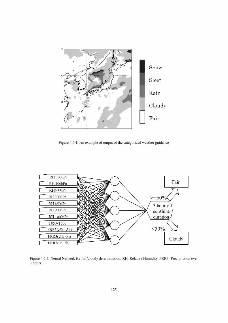
Figure 4.6.4: An example of output of the categorized weather guidance

Figure 4.6.5: Neural Network for fair/cloudy determination. RH: Relative Humidity, FRR3: Precipitation over3 hours.

125

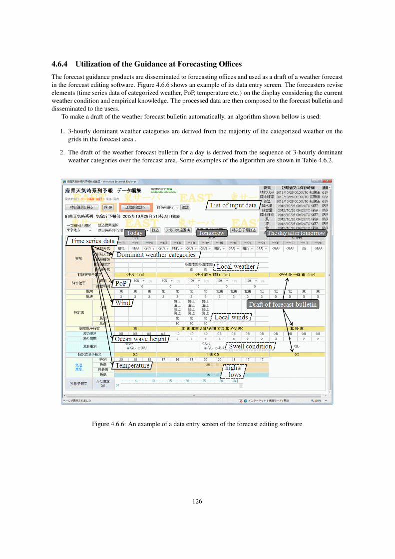
4.6.4 Utilization of the Guidance at Forecasting OfficesThe forecast guidance products are disseminated to forecasting offices and used as a draft of a weather forecastin the forecast editing software. Figure 4.6.6 shows an example of its data entry screen. The forecasters reviseelements (time series data of categorized weather, PoP, temperature etc.) on the display considering the currentweather condition and empirical knowledge. The processed data are then composed to the forecast bulletin anddisseminated to the users.

To make a draft of the weather forecast bulletin automatically, an algorithm shown bellow is used:

1. 3-hourly dominant weather categories are derived from the majority of the categorized weather on thegrids in the forecast area .

2. The draft of the weather forecast bulletin for a day is derived from the sequence of 3-hourly dominantweather categories over the forecast area. Some examples of the algorithm are shown in Table 4.6.2.

Figure 4.6.6: An example of a data entry screen of the forecast editing software

126

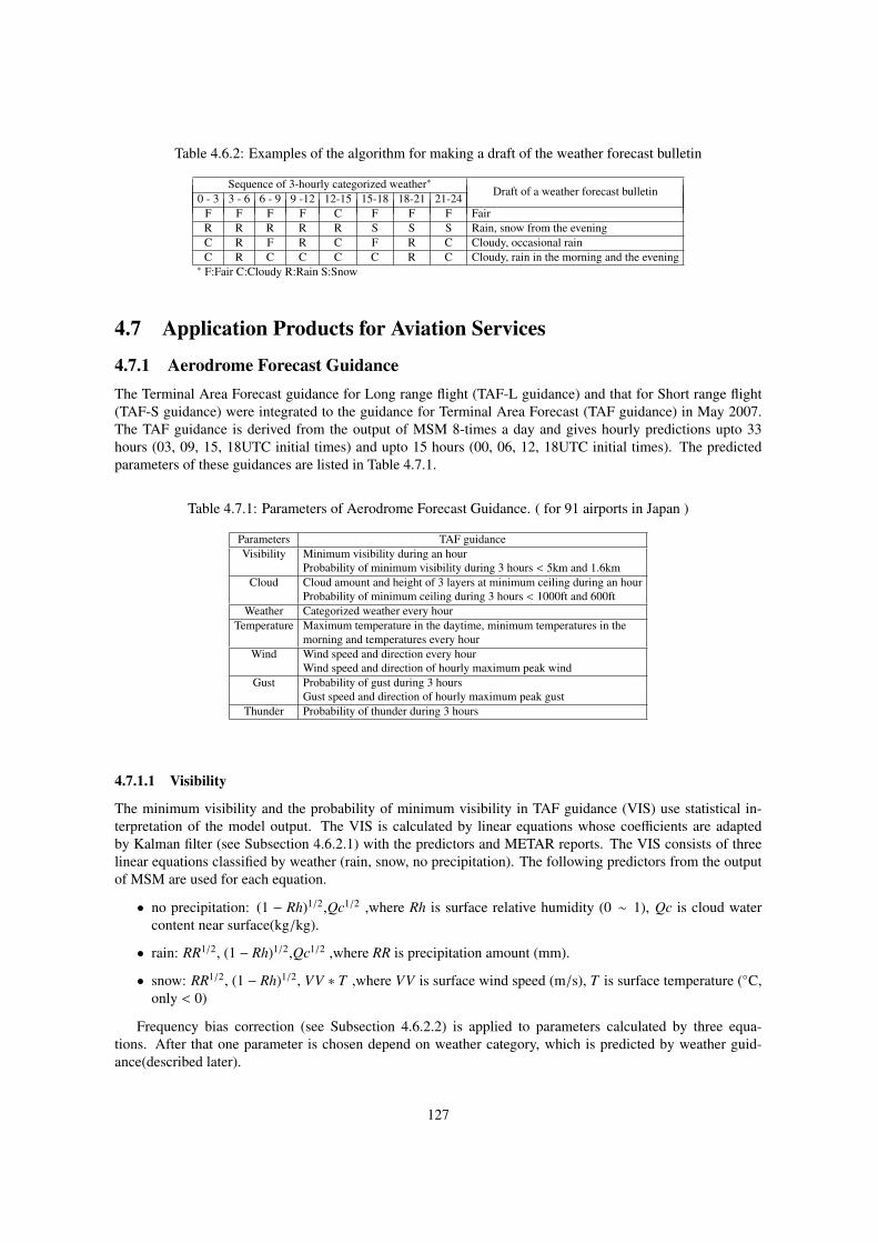
Table 4.6.2: Examples of the algorithm for making a draft of the weather forecast bulletin

Sequence of 3-hourly categorized weather∗Draft of a weather forecast bulletin

0 - 3 3 - 6 6 - 9 9 -12 12-15 15-18 18-21 21-24F F F F C F F F FairR R R R R S S S Rain, snow from the eveningC R F R C F R C Cloudy, occasional rainC R C C C C R C Cloudy, rain in the morning and the evening∗ F:Fair C:Cloudy R:Rain S:Snow

4.7 Application Products for Aviation Services

4.7.1 Aerodrome Forecast GuidanceThe Terminal Area Forecast guidance for Long range flight (TAF-L guidance) and that for Short range flight(TAF-S guidance) were integrated to the guidance for Terminal Area Forecast (TAF guidance) in May 2007.The TAF guidance is derived from the output of MSM 8-times a day and gives hourly predictions upto 33hours (03, 09, 15, 18UTC initial times) and upto 15 hours (00, 06, 12, 18UTC initial times). The predictedparameters of these guidances are listed in Table 4.7.1.

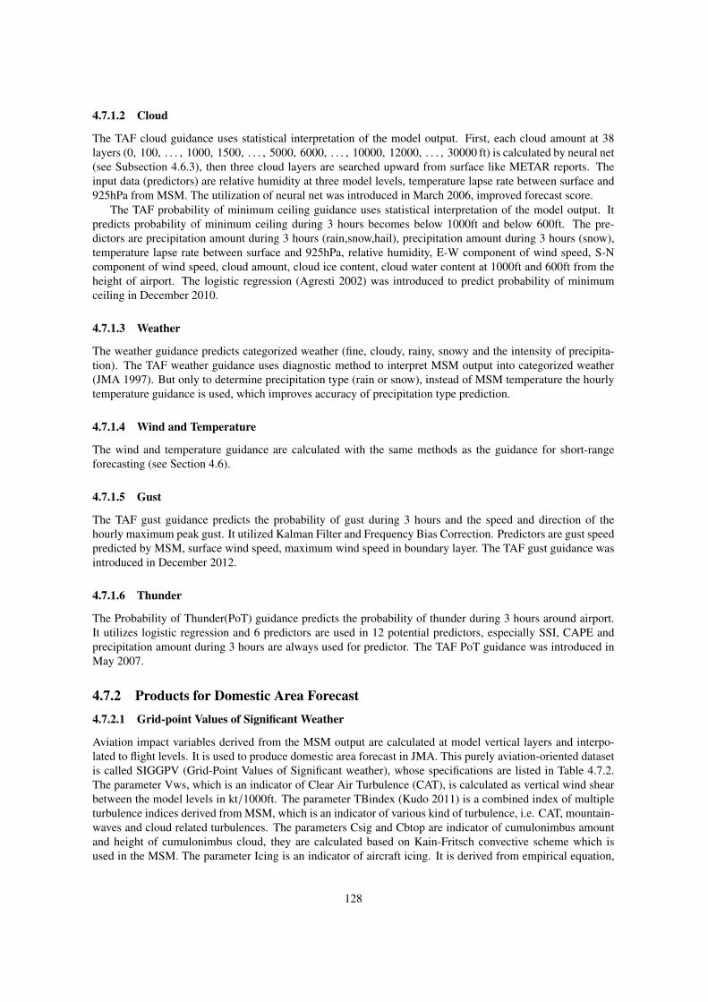
Table 4.7.1: Parameters of Aerodrome Forecast Guidance. ( for 91 airports in Japan )

Parameters TAF guidanceVisibility Minimum visibility during an hour

Probability of minimum visibility during 3 hours < 5km and 1.6kmCloud Cloud amount and height of 3 layers at minimum ceiling during an hour

Probability of minimum ceiling during 3 hours < 1000ft and 600ftWeather Categorized weather every hour

Temperature Maximum temperature in the daytime, minimum temperatures in themorning and temperatures every hour

Wind Wind speed and direction every hourWind speed and direction of hourly maximum peak wind

Gust Probability of gust during 3 hoursGust speed and direction of hourly maximum peak gust

Thunder Probability of thunder during 3 hours

4.7.1.1 Visibility

The minimum visibility and the probability of minimum visibility in TAF guidance (VIS) use statistical in-terpretation of the model output. The VIS is calculated by linear equations whose coefficients are adaptedby Kalman filter (see Subsection 4.6.2.1) with the predictors and METAR reports. The VIS consists of threelinear equations classified by weather (rain, snow, no precipitation). The following predictors from the outputof MSM are used for each equation.

• no precipitation: (1 − Rh)1/2,Qc1/2 ,where Rh is surface relative humidity (0 ∼ 1), Qc is cloud watercontent near surface(kg/kg).

• rain: RR1/2, (1 − Rh)1/2,Qc1/2 ,where RR is precipitation amount (mm).

• snow: RR1/2, (1 − Rh)1/2, VV ∗ T ,where VV is surface wind speed (m/s), T is surface temperature (C,only < 0)

Frequency bias correction (see Subsection 4.6.2.2) is applied to parameters calculated by three equa-tions. After that one parameter is chosen depend on weather category, which is predicted by weather guid-ance(described later).

127

4.7.1.2 Cloud

The TAF cloud guidance uses statistical interpretation of the model output. First, each cloud amount at 38layers (0, 100, . . . , 1000, 1500, . . . , 5000, 6000, . . . , 10000, 12000, . . . , 30000 ft) is calculated by neural net(see Subsection 4.6.3), then three cloud layers are searched upward from surface like METAR reports. Theinput data (predictors) are relative humidity at three model levels, temperature lapse rate between surface and925hPa from MSM. The utilization of neural net was introduced in March 2006, improved forecast score.

The TAF probability of minimum ceiling guidance uses statistical interpretation of the model output. Itpredicts probability of minimum ceiling during 3 hours becomes below 1000ft and below 600ft. The pre-dictors are precipitation amount during 3 hours (rain,snow,hail), precipitation amount during 3 hours (snow),temperature lapse rate between surface and 925hPa, relative humidity, E-W component of wind speed, S-Ncomponent of wind speed, cloud amount, cloud ice content, cloud water content at 1000ft and 600ft from theheight of airport. The logistic regression (Agresti 2002) was introduced to predict probability of minimumceiling in December 2010.

4.7.1.3 Weather

The weather guidance predicts categorized weather (fine, cloudy, rainy, snowy and the intensity of precipita-tion). The TAF weather guidance uses diagnostic method to interpret MSM output into categorized weather(JMA 1997). But only to determine precipitation type (rain or snow), instead of MSM temperature the hourlytemperature guidance is used, which improves accuracy of precipitation type prediction.

4.7.1.4 Wind and Temperature

The wind and temperature guidance are calculated with the same methods as the guidance for short-rangeforecasting (see Section 4.6).

4.7.1.5 Gust

The TAF gust guidance predicts the probability of gust during 3 hours and the speed and direction of thehourly maximum peak gust. It utilized Kalman Filter and Frequency Bias Correction. Predictors are gust speedpredicted by MSM, surface wind speed, maximum wind speed in boundary layer. The TAF gust guidance wasintroduced in December 2012.

4.7.1.6 Thunder

The Probability of Thunder(PoT) guidance predicts the probability of thunder during 3 hours around airport.It utilizes logistic regression and 6 predictors are used in 12 potential predictors, especially SSI, CAPE andprecipitation amount during 3 hours are always used for predictor. The TAF PoT guidance was introduced inMay 2007.

4.7.2 Products for Domestic Area Forecast4.7.2.1 Grid-point Values of Significant Weather

Aviation impact variables derived from the MSM output are calculated at model vertical layers and interpo-lated to flight levels. It is used to produce domestic area forecast in JMA. This purely aviation-oriented datasetis called SIGGPV (Grid-Point Values of Significant weather), whose specifications are listed in Table 4.7.2.The parameter Vws, which is an indicator of Clear Air Turbulence (CAT), is calculated as vertical wind shearbetween the model levels in kt/1000ft. The parameter TBindex (Kudo 2011) is a combined index of multipleturbulence indices derived from MSM, which is an indicator of various kind of turbulence, i.e. CAT, mountain-waves and cloud related turbulences. The parameters Csig and Cbtop are indicator of cumulonimbus amountand height of cumulonimbus cloud, they are calculated based on Kain-Fritsch convective scheme which isused in the MSM. The parameter Icing is an indicator of aircraft icing. It is derived from empirical equation,

128

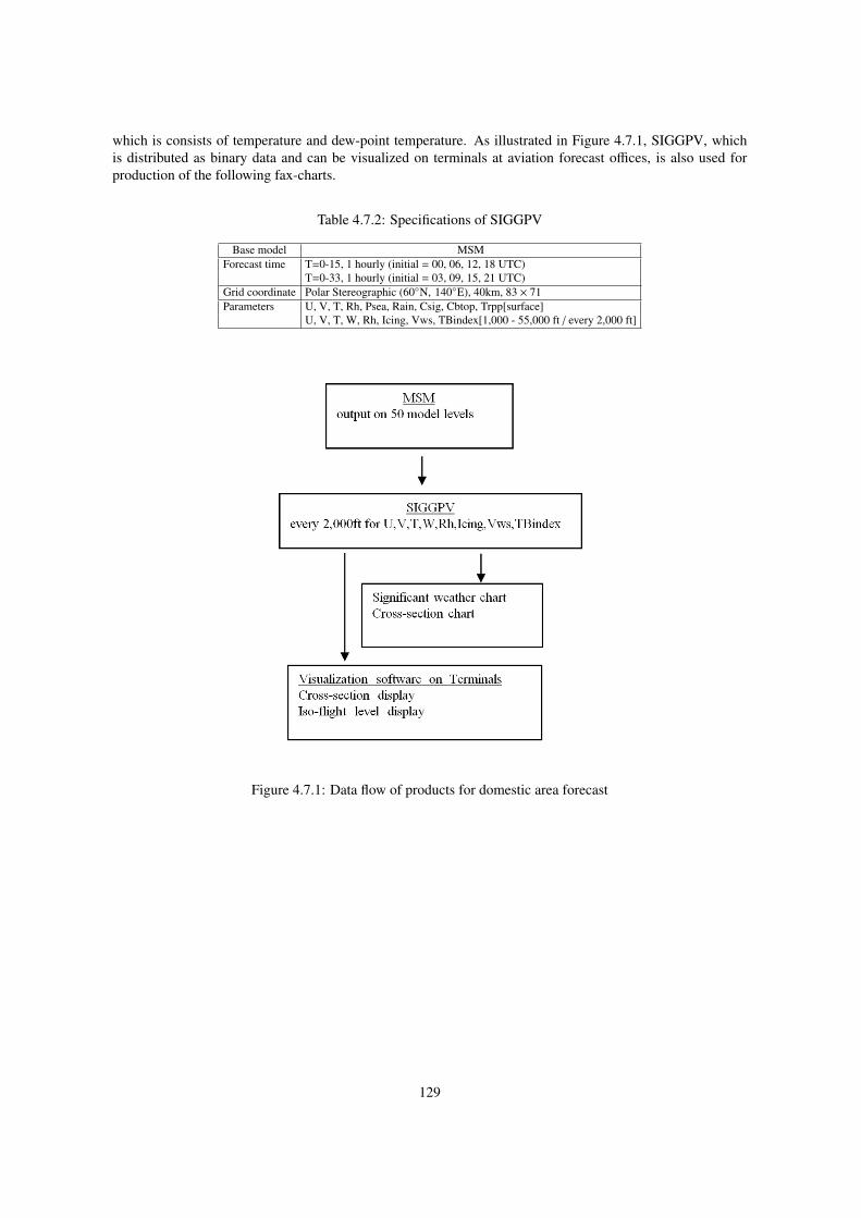
which is consists of temperature and dew-point temperature. As illustrated in Figure 4.7.1, SIGGPV, whichis distributed as binary data and can be visualized on terminals at aviation forecast offices, is also used forproduction of the following fax-charts.

Table 4.7.2: Specifications of SIGGPV

Base model MSMForecast time T=0-15, 1 hourly (initial = 00, 06, 12, 18 UTC)

T=0-33, 1 hourly (initial = 03, 09, 15, 21 UTC)Grid coordinate Polar Stereographic (60N, 140E), 40km, 83 × 71Parameters U, V, T, Rh, Psea, Rain, Csig, Cbtop, Trpp[surface]

U, V, T, W, Rh, Icing, Vws, TBindex[1,000 - 55,000 ft / every 2,000 ft]

Figure 4.7.1: Data flow of products for domestic area forecast

129

4.7.2.2 Domestic Significant Weather Chart

Figure 4.7.2: An example of the domestic significant weather chart

This chart shows 12- hour forecast fields of the parameters listed below in four panels: (Figure 4.7.2)

• Upper-left:

– Jet stream axes.

– Possible CAT areas.

– Possible Cb areas.

• Lower-left:

– Contours of 0C height.

– Possible icing areas at 500, 700 and 850hPa based on the -8 D method (Godske 1957)

• Upper-right:

– Contours of sea level pressure.

– Moist areas at 700 hPa.

– Front parameters DDT = −∇n|∇nT |, where T is mean temperature below 500hPa and ∇n denotesthe horizontal gradient perpendicular to the isotherms.

130

– “NP fronts” drawn along the maxima of DDT .

• Lower-right:

– Cloud indices indicating the low, middle and upper cloud amount.

4.7.2.3 Domestic Cross-section Chart

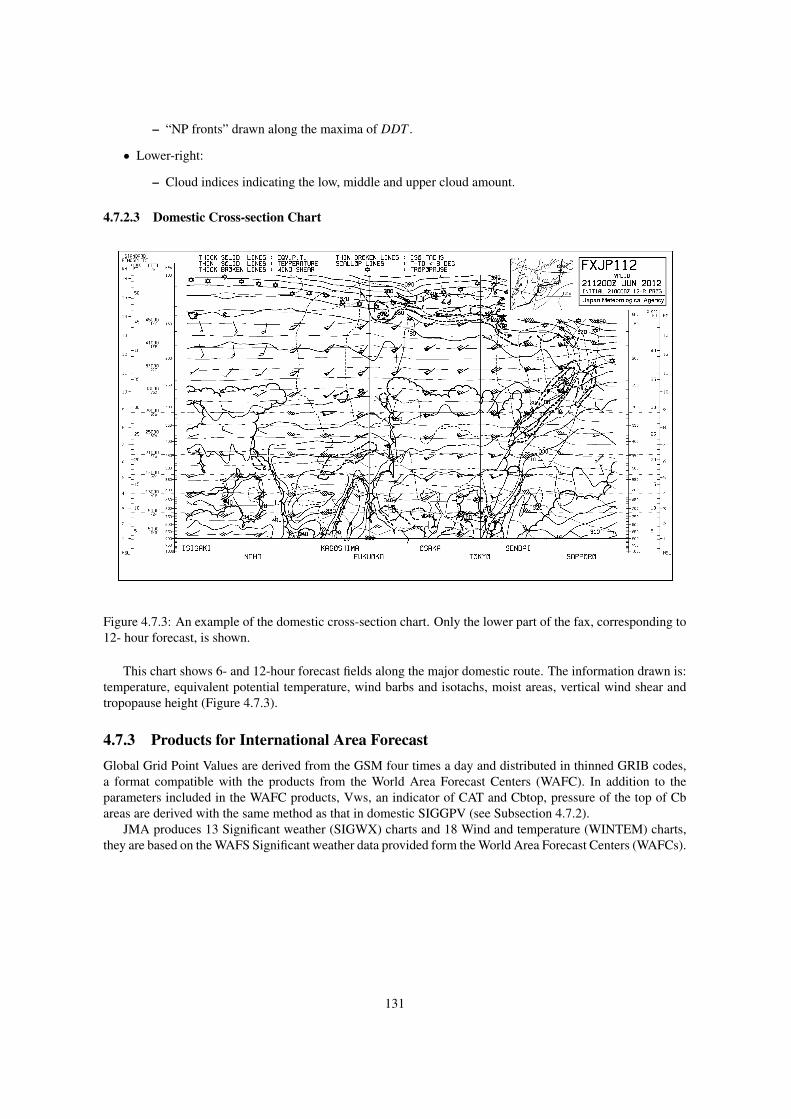
Figure 4.7.3: An example of the domestic cross-section chart. Only the lower part of the fax, corresponding to12- hour forecast, is shown.

This chart shows 6- and 12-hour forecast fields along the major domestic route. The information drawn is:temperature, equivalent potential temperature, wind barbs and isotachs, moist areas, vertical wind shear andtropopause height (Figure 4.7.3).

4.7.3 Products for International Area ForecastGlobal Grid Point Values are derived from the GSM four times a day and distributed in thinned GRIB codes,a format compatible with the products from the World Area Forecast Centers (WAFC). In addition to theparameters included in the WAFC products, Vws, an indicator of CAT and Cbtop, pressure of the top of Cbareas are derived with the same method as that in domestic SIGGPV (see Subsection 4.7.2).

JMA produces 13 Significant weather (SIGWX) charts and 18 Wind and temperature (WINTEM) charts,they are based on the WAFS Significant weather data provided form the World Area Forecast Centers (WAFCs).

131

4.8 Products of Ensemble Prediction System

4.8.1 Products of the EPS for One-week ForecastingTo assist forecasters in issuing one-week weather forecasts, some products of ensemble mean are made fromoutput of the EPS.

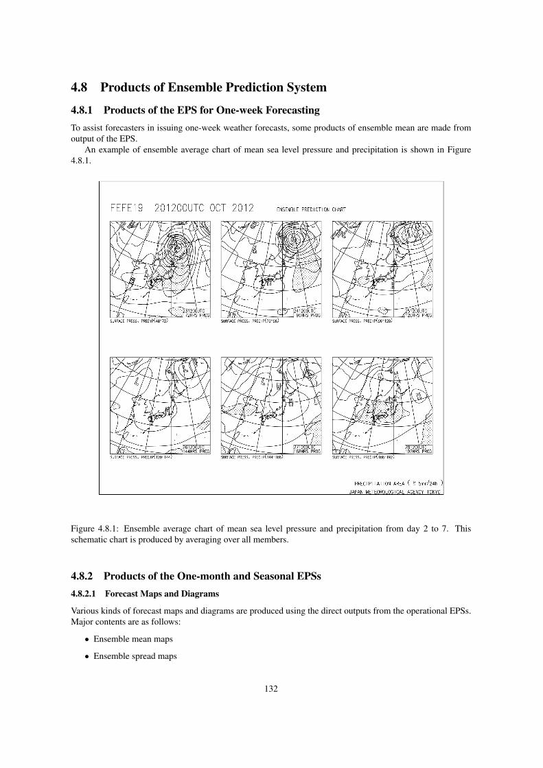
An example of ensemble average chart of mean sea level pressure and precipitation is shown in Figure4.8.1.

Figure 4.8.1: Ensemble average chart of mean sea level pressure and precipitation from day 2 to 7. Thisschematic chart is produced by averaging over all members.

4.8.2 Products of the One-month and Seasonal EPSs4.8.2.1 Forecast Maps and Diagrams

Various kinds of forecast maps and diagrams are produced using the direct outputs from the operational EPSs.Major contents are as follows:

• Ensemble mean maps

• Ensemble spread maps

132

• Diagrams of time series of varies indices calculated from the ensemble mean and the individual memberforecasts (for domestic users only)

• Outlook of sea surface temperature deviations for Nino regions to support monthly El Nino outlook(Figure 4.8.2)

4.8.2.2 Gridded Data

Gridded data of the model output has been provided via the TCC (the Tokyo Climate Center) website. Theproducts are as follows:

• One-month EPS

– Daily mean ensemble statistics

– Daily mean forecast of the individual ensemble member

• Seasonal EPS

– Monthly mean ensemble statistics

– Monthly mean forecast of the individual ensemble member

4.8.2.3 Probabilistic Forecast Products

Probabilistic forecasts of three-category (e.g., above-, near-, below-normal) and probabilistic distribution func-tions are produced using the direct model outputs and hindcast datasets (Figure 4.8.3).

4.8.2.4 Hindcast Dataset and Verification Results

A hindcast is a long set of systematic forecast experiments for past cases, and is performed using forecastmodels identical to the current operational version. JMA provides not only the operational products but alsothe hindcast dataset. The Hindcast datasets are used statistically to calibrate real-time forecasts and to evaluatethe prediction skill of models.

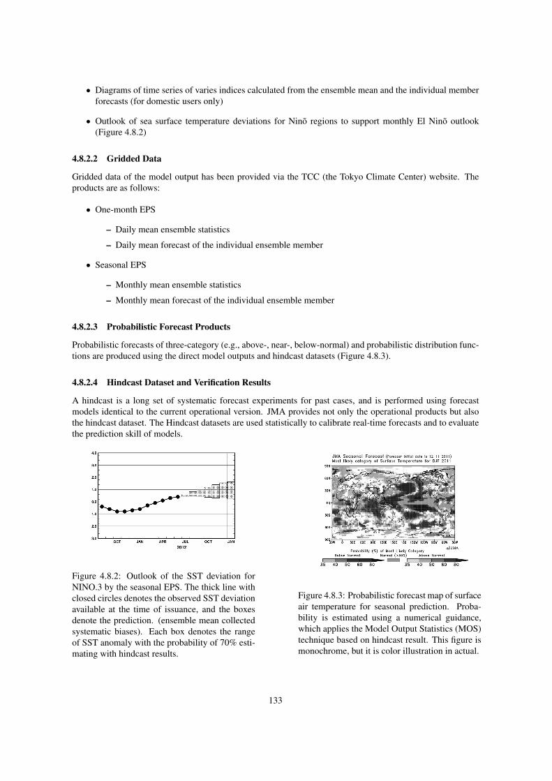
Figure 4.8.2: Outlook of the SST deviation forNINO.3 by the seasonal EPS. The thick line withclosed circles denotes the observed SST deviationavailable at the time of issuance, and the boxesdenote the prediction. (ensemble mean collectedsystematic biases). Each box denotes the rangeof SST anomaly with the probability of 70% esti-mating with hindcast results.

Figure 4.8.3: Probabilistic forecast map of surfaceair temperature for seasonal prediction. Proba-bility is estimated using a numerical guidance,which applies the Model Output Statistics (MOS)technique based on hindcast result. This figure ismonochrome, but it is color illustration in actual.

133

4.9 Atmospheric Angular Momentum FunctionsThe Atmospheric Angular Momentum (AAM) functions were proposed to evaluate the earth rotational varia-tion by precisely estimating the variation of the atmospheric angular momentum. To monitor the atmosphericeffect on the earth rotation, JMA sends the AAM products to NCEP which is the sub-bureau of InternationalEarth Rotation Service (IERS) through GTS. The AAM functions are expressed as follows (Barnes et al. 1983).

χ1 = − 1.00[

r2

(C − A)g

] ∫PS sin φ cos φ cos λ dS

− 1.43[

rΩ(C − A)g

]"(u sin φ cos λ − v sin λ) dPdS , (4.9.1)

χ2 = − 1.00[

r2

(C − A)g

] ∫PS sin φ cos φ sin λ dS

− 1.43[

rΩ(C − A)g

]"(u sin φ sin λ + v cos λ) dPdS , (4.9.2)

χ3 = − 0.70[

r2

Cg

] ∫PS cos2 φ dS − 1.00

[rΩCg

]"u cos φ dPdS . (4.9.3)

In Eq. (4.9.1) to Eq. (4.9.3), P is the pressure,∫

dS is the surface integral over the globe, (φ, λ) are latitudeand longitude, u, v are the eastward and northward components of the wind velocity, PS is the surface pressure,g is the mean acceleration of gravity, r is the mean radius of the earth, C is the polar moment of inertia of thesolid earth, A is the equatorial moment of inertia, and Ω is the mean angular velocity of the earth.

Functions χ1 and χ2 are the equatorial, and function χ3 is the axial component. Every component is non-dimensional. The first term of each component is a pressure-term, which is related to the redistribution ofthe air masses. The second term is a wind-term, which is related to the relative angular momentum of theatmosphere.

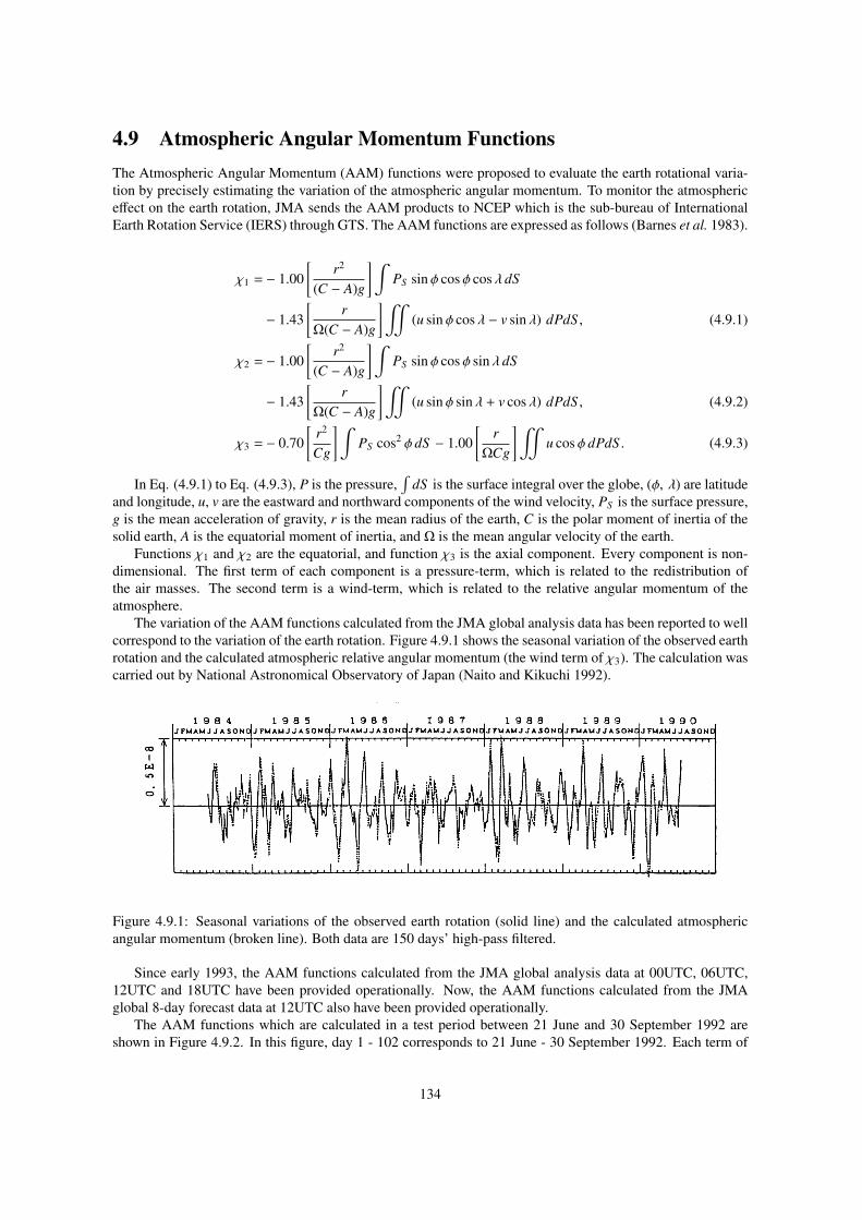
The variation of the AAM functions calculated from the JMA global analysis data has been reported to wellcorrespond to the variation of the earth rotation. Figure 4.9.1 shows the seasonal variation of the observed earthrotation and the calculated atmospheric relative angular momentum (the wind term of χ3). The calculation wascarried out by National Astronomical Observatory of Japan (Naito and Kikuchi 1992).

Figure 4.9.1: Seasonal variations of the observed earth rotation (solid line) and the calculated atmosphericangular momentum (broken line). Both data are 150 days’ high-pass filtered.

Since early 1993, the AAM functions calculated from the JMA global analysis data at 00UTC, 06UTC,12UTC and 18UTC have been provided operationally. Now, the AAM functions calculated from the JMAglobal 8-day forecast data at 12UTC also have been provided operationally.

The AAM functions which are calculated in a test period between 21 June and 30 September 1992 areshown in Figure 4.9.2. In this figure, day 1 - 102 corresponds to 21 June - 30 September 1992. Each term of

134

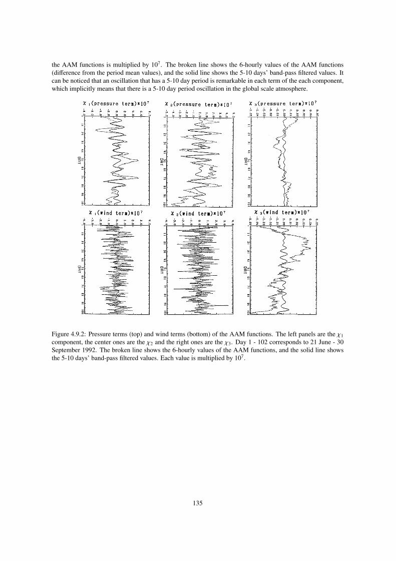
the AAM functions is multiplied by 107. The broken line shows the 6-hourly values of the AAM functions(difference from the period mean values), and the solid line shows the 5-10 days’ band-pass filtered values. Itcan be noticed that an oscillation that has a 5-10 day period is remarkable in each term of the each component,which implicitly means that there is a 5-10 day period oscillation in the global scale atmosphere.

Figure 4.9.2: Pressure terms (top) and wind terms (bottom) of the AAM functions. The left panels are the χ1component, the center ones are the χ2 and the right ones are the χ3. Day 1 - 102 corresponds to 21 June - 30September 1992. The broken line shows the 6-hourly values of the AAM functions, and the solid line showsthe 5-10 days’ band-pass filtered values. Each value is multiplied by 107.

135

136