Embed Size (px)
Citation preview
AQUIFER FLUID MODELLING AND ASSESSMENT OFMINERAL-GAS-LIQUID EQUILIBRIA IN THE
NÁMAFJALL GEOTHERMAL SYSTEM, NE-ICELAND
GEOTHERMAL TRAINING PROGRAMME
Sylvia Joan Malimo
Report 3November 2012
Hot spring at Ölkelduháls in the Hengill area
GEOTHERMAL TRAINING PROGRAMME Reports 2012 Orkustofnun, Grensásvegur 9, Number 3 IS-108 Reykjavík, Iceland
AQUIFER FLUID MODELLING AND ASSESSMENT OF MINERAL-GAS-LIQUID EQUILIBRIA IN THE
NÁMAFJALL GEOTHERMAL SYSTEM, NE-ICELAND
MSc thesis School of Engineering and Natural Sciences
Faculty of Earth Sciences University of Iceland
by
Sylvia Joan Malimo Geothermal Development Company Ltd - GDC
P.O. Box 17700 - 20100 Nakuru
KENYA [email protected], [email protected]
United Nations University Geothermal Training Programme
Reykjavík, Iceland Published in November 2012
ISBN 978-9979-68-322-3
ISSN 1670-7427

ii
This MSc thesis has also been published in April 2012 by the School of Engineering and Natural Sciences,
Faculty of Earth Sciences University of Iceland

iii
INTRODUCTION
The Geothermal Training Programme of the United Nations University (UNU) has operated in Iceland since 1979 with six month annual courses for professionals from developing countries. The aim is to assist developing countries with significant geothermal potential to build up groups of specialists that cover most aspects of geothermal exploration and development. During 1979-2012, 515 scientists and engineers from 53 developing countries have completed the six month courses. They have come from Asia (40%), Africa (32%), Central America (16%), Central and Eastern Europe (12%), and Oceania (0.4%) There is a steady flow of requests from all over the world for the six month training and we can only meet a portion of the requests. Most of the trainees are awarded UNU Fellowships financed by the UNU and the Government of Iceland. Candidates for the six month specialized training must have at least a BSc degree and a minimum of one year practical experience in geothermal work in their home countries prior to the training. Many of our trainees have already completed their MSc or PhD degrees when they come to Iceland, but several excellent students who have only BSc degrees have made requests to come again to Iceland for a higher academic degree. In 1999, it was decided to start admitting UNU Fellows to continue their studies and study for MSc degrees in geothermal science or engineering in co-operation with the University of Iceland. An agreement to this effect was signed with the University of Iceland. The six month studies at the UNU Geothermal Training Programme form a part of the graduate programme.
It is a pleasure to introduce the 31st UNU Fellow to complete the MSc studies at the University of Iceland under the co-operation agreement. Sylvia J. Malimo, BSc in Chemistry and Mathematics, of the Geothermal Development Company – GDC, Kenya, completed the six month specialized training in Chemistry of Thermal Fluids at the UNU Geothermal Training Programme in October 2009. Her research report was entitled: “Interpretation of geochemical well test data for wells OW-903B, OW-904B and OW-909, Olkaria Domes, Kenya”. After one year of geothermal research work in Kenya, she came back to Iceland for MSc studies at the Faculty of Earth Sciences of the University of Iceland in August 2010. In April 2012, she defended her MSc thesis presented here, entitled “Aquifer fluid modelling and assessment of mineral-gas-liquid equilibria in the Námafjall geothermal system, NE-Iceland”. Her studies in Iceland were financed by the Government of Iceland through a UNU-GTP Fellowship from the UNU Geothermal Training Programme. We congratulate her on her achievements and wish her all the best for the future. We thank the Faculty of Earth Sciences at the School of Engineering and Natural Sciences of the University of Iceland for the co-operation, and her supervisors for the dedication. Finally, I would like to mention that Sylvia’s MSc thesis with the figures in colour is available for downloading on our website www.unugtp.is under publications.
With warmest wishes from Iceland,
Ingvar B. Fridleifsson, director United Nations University Geothermal Training Programme

iv
ACKNOWLEDGEMENTS I acknowledge and thank the following for their support and contributions to this study: … Government of Iceland for awarding me this Fellowship through the United Nations University Geothermal Training Programme (UNU-GTP). … UNU-GTP staff: Ingvar Birgir Fridleifsson, Lúdvík S. Georgsson, Thórhildur Ísberg, Ingimar G. Haraldsson, Markús A.G. Wilde and Málfrídur Ómarsdóttir. … Geothermal Development Company Ltd., Kenya for granting me the time off work to pursue this study. … To my supervisors: Dr. Thráinn Fridriksson and Prof. Stefán Arnórsson who have had the enthusiasm and made the time for discussions towards this study. Your views and eagerness to provide me with meticulous comments on the principles in the chapters have been admirable, and certainly contributed to a clearer presentation of ideas. … Landsvirkjun, Orkustofnun, ÍSOR and Kemia Ltd for providing the data on which this study is based. … Dr. Andri Stefánsson and Nicole Keller at the Institute of Earth Sciences, University of Iceland for various inputs and discussions. … Orkustofnun and ÍSOR staff with special thanks to Rósa S. Jónsdóttir, Magnús Ólafsson and Sigrídur Sif Gylfadóttir. My family and friends for their love, support and encouragement.
DEDICATION
For Rhoda James, my "antique" girl.

v
ABSTRACT This study presents a geochemical evaluation of the Námafjall high-temperature geothermal field with respect to the chemical and physical processes that account for the fluid concentrations of volatile and non-volatile components, and the mineral assemblages controlling equilibrium in the aquifer. Aquifer fluid compositions and aqueous species distribution, for 25 samples collected from 7 wet-steam well discharges, were calculated from water- and steam-phase analyses and discharge enthalpies using the WATCH 2.1 speciation program according to the phase segregation model. Phase segregation pressures calculated at ~80% volume fraction of the flowing vapour are selected in view of the fact that liquid saturation at this pressures relate to residual liquid saturation of 0.2. The modelled aquifer fluid compositions were used to assess how closely equilibrium is approached between solution and various minerals. H2S and H2 concentrations were used to evaluate the presence of equilibrium vapour fraction in the initial aquifer fluid, calculated as 0-3.9% by weight with a field average of 0.79% by weight. At inferred Námafjall aquifer temperatures (200-300°C), the concentration of H2S in the initial aquifer fluids is somewhat higher than predicted at equilibrium with hydrothermal mineral assemblage consisting of pyrite, pyrrhotite, prehnite and epidote, while concentration of H2 closely approaches equilibrium for the excess enthalpy wells unlike for the liquid enthalpy wells. With respect to CO2 the calculated chemical compositions of initial aquifer fluid show a close approach to equilibrium (for liquid enthalpy wells) but lower than equilibrium for the excess enthalpy wells with the hydrothermal alteration minerals clinozoisite, calcite, quartz and prehnite. The shallower aquifer at Námafjall are higher in gas (H2S, H2, CO2 and N2) indicating that gaseous steam from deeper aquifers has condensed in the shallower ones signifying that they are, at least partly, steam-heated. The main uncertainty involved in calculating mineral saturation indices, particularly in the case of excess enthalpy well discharges, lies in the model adopted to calculate the aquifer water composition and its aqueous species distribution and in the quality of the thermodynamic data on the aqueous species and the minerals especially those that involve Fe-bearing species. In the deep aquifers, chemical equilibrium has been rather closely approached between dissolved solids, H2S and H2 on one hand and hydrothermal minerals on the other.
vi
TABLE OF CONTENTS Page 1. INTRODUCTION ......................................................................................................................... 1 2. NÁMAFJALL GEOTHERMAL FIELD ....................................................................................... 5 2.1 Geology... ............................................................................................................................. 5 2.2 Hydrology ............................................................................................................................ 7 2.3 Geophysical review.............................................................................................................. 8 2.4 Geochemical review ............................................................................................................ 9 2.5 Reservoir characteristics .................................................................................................... 11 3. METHODOLOGY ....................................................................................................................... 12 3.1 Sampling and analysis ....................................................................................................... 12 3.2 Data handling ..................................................................................................................... 14 3.3 Aquifer fluid modelling ..................................................................................................... 14 3.3.1 ‘Excess’ enthalpy and phase segregation ........................................................... 14 3.3.2 Aquifer fluid temperature ................................................................................... 16 3.3.3 Phase segregation pressure ................................................................................. 19 3.3.4 Thermodynamics of the phase segregation model ............................................. 21 3.4 Equilibrium vapour fraction ............................................................................................... 30 4. MINERAL-GAS-LIQUID EQUILIBRIA ................................................................................... 34 4.1 Alteration mineralogy and thermodynamic data ................................................................ 34 4.2 Mineral-gas equilibria ........................................................................................................ 37 4.2.1 H2S and H2 .......................................................................................................... 38 4.2.2 CO2 ..................................................................................................................... 39 4.3 Mineral-solute equilibria .................................................................................................... 40 4.3.1 Calcite, wollastonite and anhydrite .................................................................... 41 4.3.2 Epidote-clinozoisite, grossular and prehnite ...................................................... 42 4.3.3 Magnetite, pyrite and pyrrhotite ......................................................................... 43 5. SUMMARY AND CONCLUSIONS .......................................................................................... 46 REFERENCES ....................................................................................................................................... 49 APPENDIX I: Temperature profiles of Námafjall wells ...................................................................... 56 APPENDIX II: Fluid/gas characteristics and selected constituent concentrations at 10 bar-a ............. 57 LIST OF FIGURES 1. Simplified geological map of Iceland. ........................................................................................... 1 2. Location of wells in the Námafjall geothermal field. ..................................................................... 3 3. Structural map of Krafla and Námafjall geothermal areas ............................................................. 5 4. Geological map of the Námafjall area ........................................................................................... 6 5. Possible groundwater flow model to Námafjall and Krafla ........................................................... 7 6. General resistivity structure and alteration of basaltic crust in Iceland. ........................................ 8 7. Resistivity structure of Námafjall ................................................................................................. 9 8. Reservoir temperature contours based on geothermometry ........................................................ 10 9. Changes during the production period in the concentrations of Cl, SO4 and SiO2 at 10 bar-a .... 10 10. The basic grid of the Námafjall model ......................................................................................... 11 11. Mass recharge into the reservoir .................................................................................................. 11 12. Relationship between p/T and enthalpy of saturated steam in the range 100-300°C ................... 14
vii
Page 13. Fluid characteristics and concentration of Námafjall wells at 10 bar-a ....................................... 15 14. Discharge enthalpy of wells in Námafjall field ............................................................................ 16 15. Variation in silica content in separated waters and total discharge of excess enthalpy wells ...... 17 16. Relationship between geothermometer temperatures in Námafjall wells .................................... 18 17. Relative permeability functions relating liquid saturation to relative permeability ..................... 20 18. Calculated liquid saturation at segregation pressures considered at ~80% volume fraction ....... 20 19. Relative V , of initial inflowing aquifer fluid as a function ofh , . ............................................ 23 20. Relative calculated concentration of a non-volatile component (m , ) in initial aquifer fluid ..... 24 21. Relative calculated concentration of volatile components (m , ) in initial aquifer fluid .............. 28 22. Calculated SiO2 concentration of excess enthalpy wells in the initial aquifer fluid... ................. 29 23. Calculated concentration of volatiles (CO2, H2S and H2) in the initial aquifer fluid .................... 29 24. Calculated equilibrium vapour fractions (X , ) for Námafjall wells. .................................... 31
25. Calculated equilibrium vapour fractions,X , as a function of selected fluid temperature .. 32 26. Potential mineral buffers controlling H2S gas concentrations in the initial aquifer fluid. ........... 38 27. Potential mineral buffers controlling H2 gas concentrations in the initial aquifer fluid ............... 38 28. Potential mineral buffers controlling CO2 gas concentrations in the initial aquifer fluid. ........... 39 29. Saturation state of aquifer waters with respect to calcite, wollastonite and anhydrite ................. 41 30. Saturation state of calcite, wollastonite and anhydrite as a function of aquifer water pH ........... 42 31. Ca / [H ] activity ratios versus initial aquifer fluid temperature............................................. 42 32. Saturation indices of Ca-Al silicate minerals in the initial aquifer fluid ...................................... 43 33. Saturation indices of Fe-bearing minerals in the initial aquifer fluid........................................... 44 34. Fe(OH) /OH activity ratios versus initial aquifer fluid temperatures ...................................... 45 35. CalculatedH S/H activity ratios at equilibrium with pyr+mag and pyr+pyrr ............................ 45 LIST OF TABLES 1. Boreholes in Námafjall geothermal field. ...................................................................................... 2 2. Measured discharge enthalpies, sampling pressures and analysis of elements ............................ 13 3. Geothermometer equations valid in the range 0-350°C at ................................................... 17 4. Geothermometer temperatures (°C) and aquifer temperature logs for Námafjall wells. ............. 18 5. Conservation equations and equations to calculate individual component concentrations .......... 21 6. Henry‘s law constants and equations ........................................................................................... 25 7. Composition of initial aquifer fluid for Námafjall wells .............................................................. 27 8. Calculated equilibrium vapor fractions for Námafjall wells ........................................................ 31 9. Composition of initial aquifer liquid taking into account the presence of X , ............................ 33 10. Temperature equations for equilibrium constants for individual mineral dissolution reactions .. 35 11. Mineral pairs and assemblage reactions that control activity ratios and gas concentrations ....... 36
viii
ABBREVIATIONS μ Dynamic viscosity of phase i ρ , Liquid density at the point of phase segregation ρ , Vapour density at the point of phase segregation D Distribution coefficient for volatile species sat the point of phase segregation D Distribution coefficient for volatile species sin initial aquifer fluid h , Enthalpy of saturated liquid at sampling pressure SP(kJ/kg) h , Total enthalpy of well discharge (kJ/kg) h , Enthalpy of saturated vapour at sampling pressure SP(kJ/kg) h , Enthalpy of saturated liquid at phase segregation pressure P (kJ/kg) h , Enthalpy of saturated vapour at phase segregation pressure P (kJ/kg) h , Enthalpy of saturated liquid at initial aquifer fluid conditions (kJ/kg) h , Total enthalpy of initial aquifer fluid. If X , is assumed to be 0, h , =h , (kJ/kg) h , Enthalpy of saturated vapour at initial aquifer fluid conditions (kJ/kg) K , Henry’s Law solubility constant for volatile species s k Relative permeability of phase i k Intrinsic permeability m , Concentration of chemical component iin liquid phase at sampling pressure,SP(moles/kg) m , Concentration of chemical component iin total well discharge (moles/kg) m , Concentration of chemical component iin vapour phase at sampling pressure, SP(moles/kg) m , Concentration of chemical component i in liquid phase at phase segregation pressure P (moles/kg) m , Concentration of chemical component i in total fluid immediately before phase segregation
(moles/kg) m , Concentration of chemical component i in vapour phase at phase segregation pressure P (moles/kg) m , Concentration of chemical component i in liquid phase of initial aquifer fluid (moles/kg) m , Concentration of chemical component i in initial aquifer fluid. If X , = 0, m , = m , (moles/kg) m , Concentration of non-volatile rin total well discharge (moles/kg) m , Concentration of non-volatile rin liquid phase at phase segregation pressure P (moles/kg) m , Concentration of non-volatile species, r,in liquid phase of initial aquifer fluid (moles/kg) m , Concentration of non-volatile species, r,in total initial aquifer fluid. If X , = 0, m , = m , m , Concentration of volatile species s in total well discharge (moles/kg) m , Concentration of volatile species sin liquid phase at phase segregation pressureP (moles/kg) m , Concentration of volatile species sin liquid phase of the initial aquifer fluid (moles/kg) m , Concentration of volatile species sin total initial aquifer fluid (moles/kg) M Mass flow of phase i (kg/s) M , Mass flow of liquid in wet-steam well discharge (kg/s) M , Mass flow of liquid and steam in wet-steam well discharge (kg/s) M , Mass flow of steam in wet-steam well discharge (kg/s) M , Mass flow of boiled aquifer liquid which separates from steam flowing into well (kg/s) M , Mass flow of total initial aquifer fluid into well (kg/s) ∆p L⁄ Pressure gradient P Vapour pressure at which phase segregation is assumed to occur (bar-a) P Vapour pressure of the initial aquifer (bar-a) S , Liquid saturation at phase segregation pressure P SP Vapour pressure as read from gauge atop Webre separator (bar-g) T Temperature at phase segregation pressure P (°C) T Selected temperature of initial aquifer fluid (°C) taken as the average of T andT / .

ix
T / Fluid temperature (°C) as determined using the Na/K concentration ratio at equilibrium with pure low-albite and pure microcline according to Arnórsson and Stefánsson (1999) and Arnórsson et al. (2000) T Fluid temperature (°C) based on unionized silica concentration in water initially in equilibrium with quartz after adiabatic boiling to 180°C (10 bar-a vapour pressure) according to Gudmundsson and Arnórsson (2002) V , Relative mass of boiled water retained in aquifer upon phase segregation to well discharge (M , /M , ) V , Relative mass of total inflowing initial aquifer fluid to well discharge (M , /M , ) X , Vapour mass fraction at sampling pressure SP X , Vapour mass fraction immediately prior to phase segregation X , Vapour mass fraction present in the initial aquifer fluid X , Calculated equilibrium vapour fraction assuming equilibrium of H2S concentration in aquifer liquid phase X , Calculated equilibrium vapour fraction assuming equilibrium of H2 concentration in aquifer liquid phase X , Calculated equilibrium vapour fraction assuming equilibrium of H2S and H2 concentrations in aquifer liquid phase

x
1
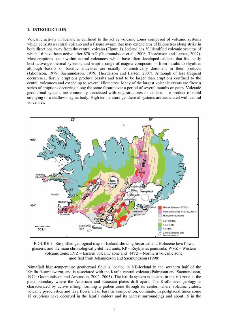
1. INTRODUCTION Volcanic activity in Iceland is confined to the active volcanic zones composed of volcanic systems which consists a central volcano and a fissure swarm that may extend tens of kilometres along strike in both directions away from the central volcano (Figure 1). Iceland has 30 identified volcanic systems of which 16 have been active after 870 AD (Gudmundsson et al., 2008; Thordarson and Larsen, 2007). Most eruptions occur within central volcanoes, which have often developed calderas that frequently host active geothermal systems, and erupt a range of magma compositions from basalts to rhyolites although basalts or basaltic andesites are usually volumetrically dominant in their products (Jakobsson, 1979; Saemundsson, 1979; Thordarson and Larsen, 2007). Although of less frequent occurrence, fissure eruptions produce basalts and tend to be larger than eruptions confined to the central volcanoes and extend up to several kilometres. Many of the largest volcanic events are fires: a series of eruptions occurring along the same fissure over a period of several months or years. Volcanic geothermal systems are commonly associated with ring structures or calderas – a product of rapid emptying of a shallow magma body. High temperature geothermal systems are associated with central volcanoes.
Námafjall high-temperature geothermal field is located in NE-Iceland in the southern half of the Krafla fissure swarm, and is associated with the Krafla central volcano (Pálmason and Saemundsson, 1974; Gudmundsson and Arnórsson, 2002; 2005). The Krafla system is located in the rift zone at the plate boundary where the American and Eurasian plates drift apart. The Krafla area geology is characterized by active rifting, forming a graben zone through its center, where volcanic craters, volcanic pyroclastics and lava flows, all of basaltic composition, dominate. In postglacial times some 18 eruptions have occurred in the Krafla caldera and its nearest surroundings and about 15 in the
FIGURE 1: Simplified geological map of Iceland showing historical and Holocene lava flows, glaciers, and the main chronologically-defined units. RP – Reykjanes peninsula; WVZ – Western
volcanic zone; EVZ – Eastern volcanic zone and NVZ – Northern volcanic zone; modified from Jóhannesson and Saemundsson (1998)
2
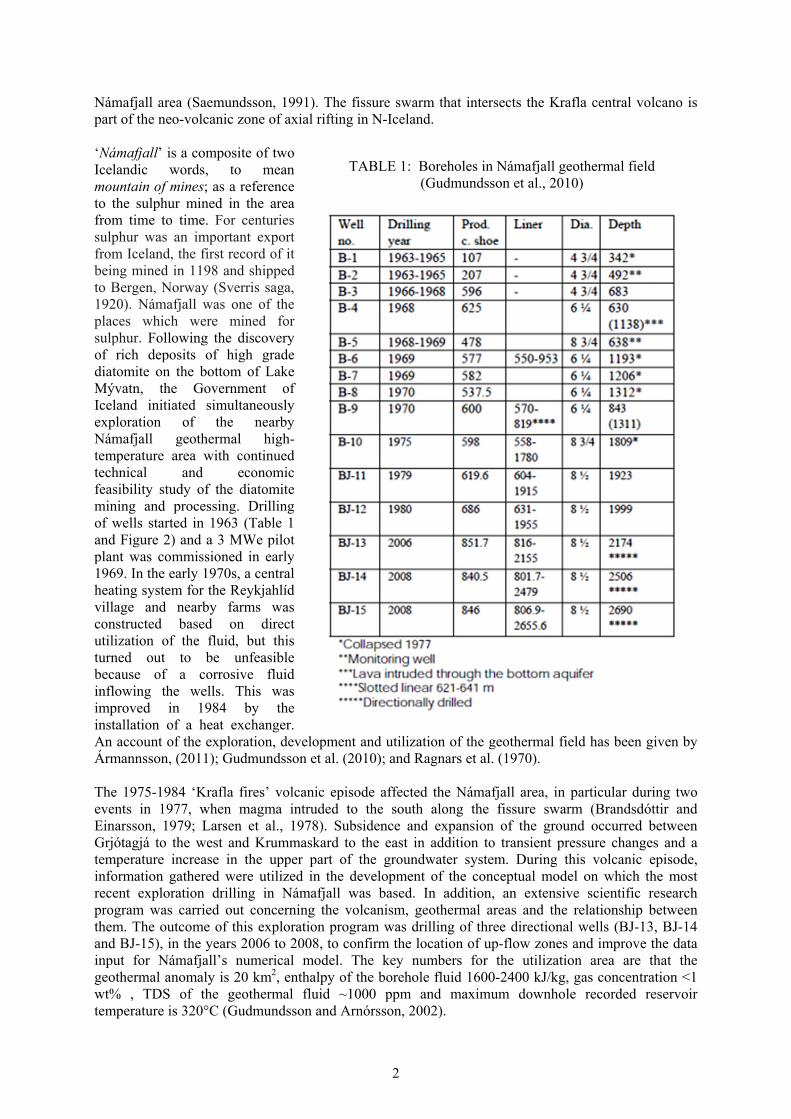
Námafjall area (Saemundsson, 1991). The fissure swarm that intersects the Krafla central volcano is part of the neo-volcanic zone of axial rifting in N-Iceland. ‘Námafjall’ is a composite of two Icelandic words, to mean mountain of mines; as a reference to the sulphur mined in the area from time to time. For centuries sulphur was an important export from Iceland, the first record of it being mined in 1198 and shipped to Bergen, Norway (Sverris saga, 1920). Námafjall was one of the places which were mined for sulphur. Following the discovery of rich deposits of high grade diatomite on the bottom of Lake Mývatn, the Government of Iceland initiated simultaneously exploration of the nearby Námafjall geothermal high-temperature area with continued technical and economic feasibility study of the diatomite mining and processing. Drilling of wells started in 1963 (Table 1 and Figure 2) and a 3 MWe pilot plant was commissioned in early 1969. In the early 1970s, a central heating system for the Reykjahlíd village and nearby farms was constructed based on direct utilization of the fluid, but this turned out to be unfeasible because of a corrosive fluid inflowing the wells. This was improved in 1984 by the installation of a heat exchanger. An account of the exploration, development and utilization of the geothermal field has been given by Ármannsson, (2011); Gudmundsson et al. (2010); and Ragnars et al. (1970). The 1975-1984 ‘Krafla fires’ volcanic episode affected the Námafjall area, in particular during two events in 1977, when magma intruded to the south along the fissure swarm (Brandsdóttir and Einarsson, 1979; Larsen et al., 1978). Subsidence and expansion of the ground occurred between Grjótagjá to the west and Krummaskard to the east in addition to transient pressure changes and a temperature increase in the upper part of the groundwater system. During this volcanic episode, information gathered were utilized in the development of the conceptual model on which the most recent exploration drilling in Námafjall was based. In addition, an extensive scientific research program was carried out concerning the volcanism, geothermal areas and the relationship between them. The outcome of this exploration program was drilling of three directional wells (BJ-13, BJ-14 and BJ-15), in the years 2006 to 2008, to confirm the location of up-flow zones and improve the data input for Námafjall’s numerical model. The key numbers for the utilization area are that the geothermal anomaly is 20 km2, enthalpy of the borehole fluid 1600-2400 kJ/kg, gas concentration <1 wt% , TDS of the geothermal fluid ~1000 ppm and maximum downhole recorded reservoir temperature is 320°C (Gudmundsson and Arnórsson, 2002).
TABLE 1: Boreholes in Námafjall geothermal field (Gudmundsson et al., 2010)
3
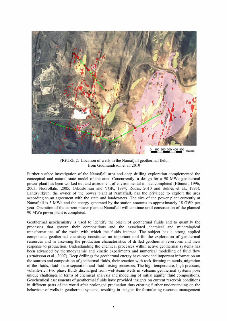
Further surface investigation of the Námafjall area and deep drilling exploration complemented the conceptual and natural state model of the area. Concurrently, a design for a 90 MWe geothermal power plant has been worked out and assessment of environmental impact completed (Hönnun, 1996; 2003; Noorollahi, 2005; Orkustofnun and VGK, 1994; Rodas, 2010 and Sólnes et al., 1995). Landsvirkjun, the owner of the power plant at Námafjall, has the privilege to exploit the area according to an agreement with the state and landowners. The size of the power plant currently at Námafjall is 3 MWe and the energy generated by the station amounts to approximately 18 GWh per year. Operation of the current power plant at Námafjall will continue until construction of the planned 90 MWe power plant is completed. Geothermal geochemistry is used to identify the origin of geothermal fluids and to quantify the processes that govern their compositions and the associated chemical and mineralogical transformations of the rocks with which the fluids interact. The subject has a strong applied component: geothermal chemistry constitutes an important tool for the exploration of geothermal resources and in assessing the production characteristics of drilled geothermal reservoirs and their response to production. Understanding the chemical processes within active geothermal systems has been advanced by thermodynamic and kinetic experiments and numerical modelling of fluid flow (Arnórsson et al., 2007). Deep drillings for geothermal energy have provided important information on the sources and composition of geothermal fluids, their reaction with rock-forming minerals, migration of the fluids, fluid phase separation and fluid mixing processes. The high-temperature, high-pressure, volatile-rich two phase fluids discharged from wet-steam wells in volcanic geothermal systems pose unique challenges in terms of chemical analysis and modelling of initial aquifer fluid compositions. Geochemical assessments of geothermal fluids have provided insights on current reservoir conditions in different parts of the world after prolonged production thus creating further understanding on the behaviour of wells in geothermal systems; resulting in insights for formulating resource management
FIGURE 2: Location of wells in the Námafjall geothermal field; from Gudmundsson et al. 2010
4
strategies (e.g. Angcoy, 2010; Arnórsson et al., 2007, 2010; Gudmundsson and Arnórsson, 2002; 2005; Karingithi, 2010; Scott, 2011). Geochemical monitoring of the Námafjall geothermal field during the last 20–25 years has revealed decreases in the Cl concentrations in the water discharged from most of the wells with more than 10 years production. The suspected cause is enhanced recharge of colder water into the producing aquifers due to depressurization by fluid withdrawal from the geothermal reservoir (Gudmundsson and Arnórsson, 2002). The incursion of cold groundwater into the reservoir was particularly intense subsequent the volcanic-rifting event in the area in 1977. Solute (quartz, Na/K, Na/K/Ca) geothermometry temperatures have decreased significantly in those wells where Cl concentrations have decreased but only to a limited extent in those wells which have remained constant in Cl. Aqueous SO4 concentrations increase as Cl concentrations decrease. Increase in SO4 concentrations is a reflection of cooling as anhydrite has retrograde solubility with respect to temperature. According to Gudmundsson and Arnórsson (2002), H2S-temperatures are similar to the solute geothermometry temperatures for wells with a single feed zone but higher for wells with multiple feeds, if the feed zones have significantly different temperatures. H2-temperatures are anomalously high for most wells due to the presence of equilibrium steam in the producing aquifers. The equilibrium steam fraction has been found to amount 0–2.2 % by weight of the aquifer fluid. The depth level of producing aquifers in individual wells at Námafjall has been evaluated by combining data on temperature and pressure logs and geothermometry results. Encounters with wells whose discharge enthalpies are higher than that of steam-saturated water at the feed zone temperature are common in the Icelandic geothermal experience. Wells with excess discharge enthalpies pose a particular challenge for those interested in modelling aquifer fluid compositions, and several non-isolated system models accounting for the boiling processes between aquifer and wellhead have been developed (Arnórsson et al., 2007; 2010). The excess discharge enthalpies are dominantly attributed to the process of phase segregation, the result of adhesion of liquid water to mineral grain surfaces due to capillary forces. The chemistry of fluids in volcanic geothermal systems should be considered in light of the heat transfer mechanism. The mechanism of heat transfer from the magma heat source of volcanic geothermal systems to the circulating fluid envisages deep circulation of fluid above and to the sides of a magmatic heat source with a thin layer between the magma and the base of fluid circulation, through which heat is transferred conductively. Some heat may also be transferred to the geothermal system by convection of saline fluids in a closed loop between the geothermal system and the magma heat source. Close proximity of the circulating fluid to the magmatic heat source also implies closeness of the circulating fluid to gaseous magma components. At magmatic temperatures, these components include H2O, CO2, SO2, H2, HCl, HF, and many metal-chloride and metal-fluoride species, which upon deposition can form ore deposits (Arnórsson et al., 2007). This study attempts to model the aquifer fluid of the Námafjall geothermal field with respect to geochemistry as aided by discharge fluid (two-phase) analysis, temperature and pressure logs, solute geothermometers, and mineral-gas and mineral-solution equilibria. Modeling will involve evaluating specific mineral-gas and mineral-solution equilibria that may potentially control the concentrations of the prevalent reactive gases (CO2, H2S and H2) in well discharges. The sensitivity of calculated aquifer fluid compositions to assumed phase segregation pressure for 4 out of the 7 wet-steam well discharges sampled at the Námafjall geothermal field since drilling to recent dates will be shown. Literature review of Námafjall geothermal field with production history are dealt with in Chapter 2. Description of phase segregation and its application in modelling aquifer fluid compositions, including physical description, supporting proof for the occurrence of phase segregation in the Námafjall field, a mathematical depiction and the practical procedure that can be used to integrate phase segregation calculations into modelling using WATCH 2.1 are dealt with in Chapter 3. Chapter 4 accounts for the thermodynamic database used to model aquifer mineral-gas-solution equilibria, presents the state of chemical equilibria between the main hydrothermal alteration minerals and solution, and discusses the results obtained from the modelling. Chapter 5 presents my conclusions.

5
2. NÁMAFJALL GEOTHERMAL FIELD 2.1 Geology
As mentioned in the introductory chapter, Námafjall high-temperature geothermal field is located in NE-Iceland about 5 km northeast of Lake Mývatn in the southern half of the Krafla fissure swarm, at an elevation of 300-400 m.a.s.l., and is associated with the Krafla central volcano (Pálmason and Saemundsson, 1974). The Krafla system is located in the rift zone at the plate boundary where the American and Eurasian plates drift apart. The Krafla area geology is characterized by active rifting, forming a graben zone through its center, where volcanic craters, volcanic pyroclastics and lava flows, all of basaltic composition, dominate. In postglacial times some 18 eruptions have occurred in the Krafla caldera and its nearest surroundings and about 15 in the Námafjall area. The fissure swarm that intersects the Krafla central volcano (100 km long and 5 to 8 km wide) is part of the neo-volcanic zone of axial rifting in N-Iceland (Figures 3 and 4, Saemundsson, 1991). Námafjall geothermal system is perceived a parasitic system to the Krafla field (Arnórsson, 1995): magma from the Krafla caldera travelled horizontally in the SSW direction along the fissures and fractures all the way down to Námafjall, serving as the heat source for the hydrothermal system. Supporting evidence for this is that during the Krafla eruption in 1977, well BN-04 in Námafjall discharged magma (Larsen et al., 1978). The 1975-84 volcanic episode suggests that the heat source to the Námafjall geothermal system is characterized by dykes formed by magma intrusion into tensional fissures from the magma body in the roots of the Krafla system. The aquifer rock at Námafjall is the same as at Krafla (basaltic, sub-aerially erupted lavas, sub-glacially erupted hyaloclastites, and small intrusive bodies of basalt, dolerite, gabbro and granophyres) except that silicic rocks are absent. Intrusive formations dominate below about 1500 m depth. The Námafjall field is characterized by the Námafjall ridge - about 2.5 km long and 0.5 km wide - composed of hyaloclastites formed during the last glaciation period as a product of sub-glacial eruptions. The sides of the Námafjall ridge are covered with postglacial basaltic flows, coming from
FIGURE 3: Structural map of Krafla and Námafjall
geothermal areas showing the Krafla caldera and associated fissure swarm. Based on mapping by Saemundsson (1991)
6
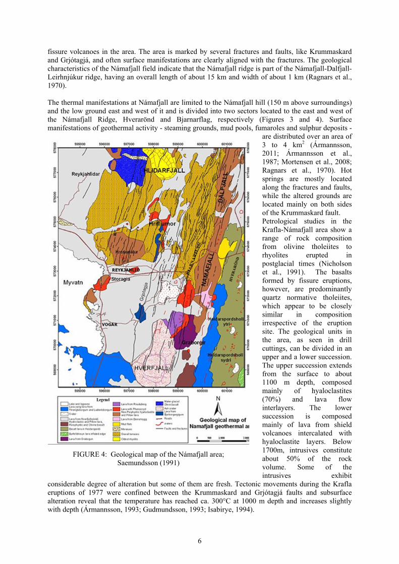
fissure volcanoes in the area. The area is marked by several fractures and faults, like Krummaskard and Grjótagjá, and often surface manifestations are clearly aligned with the fractures. The geological characteristics of the Námafjall field indicate that the Námafjall ridge is part of the Námafjall-Dalfjall-Leirhnjúkur ridge, having an overall length of about 15 km and width of about 1 km (Ragnars et al., 1970). The thermal manifestations at Námafjall are limited to the Námafjall hill (150 m above surroundings) and the low ground east and west of it and is divided into two sectors located to the east and west of the Námafjall Ridge, Hverarönd and Bjarnarflag, respectively (Figures 3 and 4). Surface manifestations of geothermal activity - steaming grounds, mud pools, fumaroles and sulphur deposits -
are distributed over an area of 3 to 4 km2 (Ármannsson, 2011; Ármannsson et al., 1987; Mortensen et al., 2008; Ragnars et al., 1970). Hot springs are mostly located along the fractures and faults, while the altered grounds are located mainly on both sides of the Krummaskard fault. Petrological studies in the Krafla-Námafjall area show a range of rock composition from olivine tholeiites to rhyolites erupted in postglacial times (Nicholson et al., 1991). The basalts formed by fissure eruptions, however, are predominantly quartz normative tholeiites, which appear to be closely similar in composition irrespective of the eruption site. The geological units in the area, as seen in drill cuttings, can be divided in an upper and a lower succession. The upper succession extends from the surface to about 1100 m depth, composed mainly of hyaloclastites (70%) and lava flow interlayers. The lower succession is composed mainly of lava from shield volcanoes intercalated with hyaloclastite layers. Below 1700m, intrusives constitute about 50% of the rock volume. Some of the intrusives exhibit
considerable degree of alteration but some of them are fresh. Tectonic movements during the Krafla eruptions of 1977 were confined between the Krummaskard and Grjótagjá faults and subsurface alteration reveal that the temperature has reached ca. 300°C at 1000 m depth and increases slightly with depth (Ármannsson, 1993; Gudmundsson, 1993; Isabirye, 1994).
FIGURE 4: Geological map of the Námafjall area; Saemundsson (1991)

7
2.2 Hydrology The surface rocks in the study area are highly permeable, consisting of recently formed lava fields where surface runoff is almost negligible. There is hardly any surface water in the area because it is covered by young and porous lava fields and transacted by numerous faults. Almost no creeks and rivers exist and nearly all the precipitation within the area seeps underground. The water is exposed in depressions where the land surface intersects the groundwater table or where aquifers are interrupted by tectonic faults and fissures (Kristmannsdóttir and Ármannsson, 2004). Part of Lake Mývatn is located in the study area. Lake Mývatn is a fresh water lake that was protected by law in 1974, and in 1978 designated to the Ramsar list of wetlands of international importance. Numerous bays and creeks line its coastline and the lake has some fifty islands and islets. The lake has an average depth of 2.5 m, and a maximum depth of 4 m. Moreover there are small lakes and pools in the area which are important for social and environmental reasons. As seen from Figure 4, the area geology indicates that different basaltic lava flows are of postglacial age, and are bound in the north by glacial moraines, in the east by older lava flows and by the Pleistocene hyaloclastites of the Námafjall ridge (Thórarinsson, 1979). The postglacial lava flow act as good aquifers and numerous open fissures and large active faults with a NNE/SSW strike, like Grjótagjá and Stóragjá, add to the already permeable nature of the lavas. From the profiles of the boreholes that have been drilled in the area it can be concluded that the uppermost layer consists mainly of lava to a depth of 20 to 25 m. This layer is underlain by a sequence of scoria layers inter-bedded with lavas, thus acting as aquifers. Ground water will flow preferentially from north to south through the north-south faults and from east to west according to the directions of the lava flows. The scoria layers probably act as more a homogeneous aquifer (De Zeeuw and Gíslason, 1988). The flashed geothermal water at Námafjall enters the shallow groundwater system through active open faults and fissures. From Námafjall the groundwater flow in a southwesterly direction and reaches Lake Mývatn in three main tongues (Figure 5). The relation between the direction of the lava flows and the direction of groundwater flow is probably caused by the fact that fissures, which developed during the cooling of the lava, are mostly parallel to the direction of the lava flow. It might also be due to the general dip of the lava and scoria layers toward the southwest. The large NS faults like Stóragjá and Grjótagjá do not form a barrier to groundwater flow (Thórarinsson, 1979; De Zeeuw and Gislason, 1988; and Noorollahi, 2005). Measurements of the flow velocity in Grjótagjá fissure suggest that the surface flow in the top layer of the groundwater in the fissures is fast, ~3.5 m/s, but at a depth of 2-4 m the flow becomes disturbed and obvious mixing occurs (Thoroddsson and Sigbjarnarson, 1983). The groundwater chemistry studies by De Zeeuw and Gíslason (1988) show that mixing of hot and cold groundwater is only important near the hot and cold water boundary zones. Based on the value of deuterium isotopes, the origin of the geothermal fluid is considered to be precipitation at high elevation, probably in the vicinity of the Vatnajökull glacier to the south (Dyngjujökull glacier). The δ2H values of the aquifer water at Námafjall fall into two distinct groups, at about -88‰ and -100‰. Ármannsson (1993) and Darling and Ármannsson (1989) considered this,
FIGURE 5: Possible groundwater flow model to Námafjall and Krafla; modified from Gudmundsson et al., 2010
8
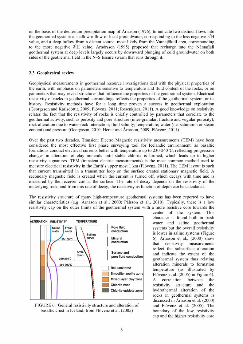
on the basis of the deuterium precipitation map of Árnason (1976), to indicate two distinct flows into the geothermal system: a shallow inflow of local groundwater, corresponding to the less negative δ2H value, and a deep inflow from a distant source, most likely from the Vatnajökull area, corresponding to the more negative δ2H value. Arnórsson (1995) proposed that recharge into the Námafjall geothermal system at deep levels largely occurs by downward plunging of cold groundwater on both sides of the geothermal field in the N–S fissure swarm that runs through it. 2.3 Geophysical review Geophysical measurements in geothermal resource investigations deal with the physical properties of the earth, with emphasis on parameters sensitive to temperature and fluid content of the rocks, or on parameters that may reveal structures that influence the properties of the geothermal system. Electrical resistivity of rocks in geothermal surroundings reflects the properties of the geothermal system, or its history. Resistivity methods have for a long time proven a success in geothermal exploration (Georgsson and Karlsdóttir, 2009; Flóvenz, 2011; Rosenkjaer, 2011). A good knowledge on resistivity relates the fact that the resistivity of rocks is chiefly controlled by parameters that correlate to the geothermal activity, such as porosity and pore structure (inter-granular, fracture and vugular porosity); rock alteration due to water-rock interaction; fluid salinity; temperature; water (i.e. saturation or steam content) and pressure (Georgsson, 2010; Hersir and Árnason, 2009; Flóvenz, 2011). Over the past two decades, Transient Electro Magnetic resistivity measurements (TEM) have been considered the most effective first phase surveying tool for Icelandic environment, as basaltic formations conduct electrical currents better with temperature up to 230-240°C, reflecting progressive changes in alteration of clay minerals until stable chlorite is formed, which leads up to higher resistivity signatures. TEM (transient electric measurements) is the most common method used to measure electrical resistivity in the Earth’s upper most 1 km (Flóvenz, 2011). The TEM layout is such that current transmitted in a transmitter loop on the surface creates stationary magnetic field. A secondary magnetic field is created when the current is turned off, which decays with time and is measured by the receiver coil at the surface. The rate of decay depends on the resistivity of the underlying rock, and from this rate of decay, the resistivity as function of depth can be calculated. The resistivity structure of many high-temperature geothermal systems has been reported to have similar characteristics (e.g. Árnason et al., 2000; Pálsson et al., 2010). Typically, there is a low resistivity cap on the outer limits of the geothermal system with a more resistive core towards the
center of the system. This character is found both in fresh water and saline geothermal systems but the overall resistivity is lower in saline systems (Figure 6). Árnason et al., (2000) show that resistivity measurements reflect the subsurface alteration and indicate the extent of the geothermal system thus relating alteration minerals to formation temperature (as illustrated by Flóvenz et al. (2005) in Figure 6). A correlation between the resistivity structure and the hydrothermal alteration of the rocks in geothermal systems is discussed in Árnason et al. (2000) and Flóvenz et al. (2005). The boundary of the low resistivity cap and the higher resistivity core
FIGURE 6: General resistivity structure and alteration of basaltic crust in Iceland; from Flóvenz et al. (2005)
9
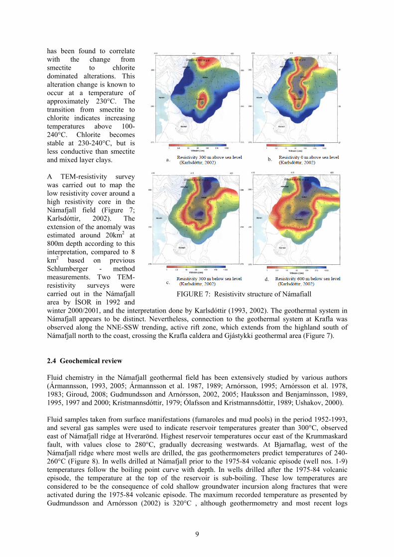
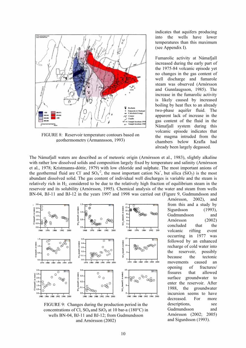
has been found to correlate with the change from smectite to chlorite dominated alterations. This alteration change is known to occur at a temperature of approximately 230°C. The transition from smectite to chlorite indicates increasing temperatures above 100-240°C. Chlorite becomes stable at 230-240°C, but is less conductive than smectite and mixed layer clays. A TEM-resistivity survey was carried out to map the low resistivity cover around a high resistivity core in the Námafjall field (Figure 7; Karlsdóttir, 2002). The extension of the anomaly was estimated around 20km2 at 800m depth according to this interpretation, compared to 8 km2 based on previous Schlumberger - method measurements. Two TEM-resistivity surveys were carried out in the Námafjall area by ÍSOR in 1992 and winter 2000/2001, and the interpretation done by Karlsdóttir (1993, 2002). The geothermal system in Námafjall appears to be distinct. Nevertheless, connection to the geothermal system at Krafla was observed along the NNE-SSW trending, active rift zone, which extends from the highland south of Námafjall north to the coast, crossing the Krafla caldera and Gjástykki geothermal area (Figure 7). 2.4 Geochemical review Fluid chemistry in the Námafjall geothermal field has been extensively studied by various authors (Ármannsson, 1993, 2005; Ármannsson et al. 1987, 1989; Arnórsson, 1995; Arnórsson et al. 1978, 1983; Giroud, 2008; Gudmundsson and Arnórsson, 2002, 2005; Hauksson and Benjamínsson, 1989, 1995, 1997 and 2000; Kristmannsdóttir, 1979; Ólafsson and Kristmannsdóttir, 1989; Ushakov, 2000). Fluid samples taken from surface manifestations (fumaroles and mud pools) in the period 1952-1993, and several gas samples were used to indicate reservoir temperatures greater than 300°C, observed east of Námafjall ridge at Hverarönd. Highest reservoir temperatures occur east of the Krummaskard fault, with values close to 280°C, gradually decreasing westwards. At Bjarnaflag, west of the Námafjall ridge where most wells are drilled, the gas geothermometers predict temperatures of 240-260°C (Figure 8). In wells drilled at Námafjall prior to the 1975-84 volcanic episode (well nos. 1-9) temperatures follow the boiling point curve with depth. In wells drilled after the 1975-84 volcanic episode, the temperature at the top of the reservoir is sub-boiling. These low temperatures are considered to be the consequence of cold shallow groundwater incursion along fractures that were activated during the 1975-84 volcanic episode. The maximum recorded temperature as presented by Gudmundsson and Arnórsson (2002) is 320°C , although geothermometry and most recent logs
FIGURE 7: Resistivity structure of Námafjall
a.
d.c.
b.
10
indicates that aquifers producing into the wells have lower temperatures than this maximum (see Appendix I). Fumarolic activity at Námafjall increased during the early part of the 1975-84 volcanic episode yet no changes in the gas content of well discharge and fumarole steam was observed (Arnórsson and Gunnlaugsson, 1985). The increase in the fumarolic activity is likely caused by increased boiling by heat flux to an already two-phase aquifer fluid. The apparent lack of increase in the gas content of the fluid in the Námafjall system during this volcanic episode indicates that the magma intruded from the chambers below Krafla had already been largely degassed.
The Námafjall waters are described as of meteoric origin (Arnórsson et al., 1983), slightly alkaline with rather low dissolved solids and composition largely fixed by temperature and salinity (Arnórsson et al., 1978; Kristmanns-dóttir, 1979) with low chloride and sulphate. The most important anions of the geothermal fluid are Cl- and SO4
-2, the most important cation Na+, but silica (SiO2) is the most abundant dissolved solid. The gas content of individual well discharges is variable and the steam is relatively rich in H2, considered to be due to the relatively high fraction of equilibrium steam in the reservoir and its solubility (Arnórsson, 1995). Chemical analysis of the water and steam from wells BN-04, BJ-11 and BJ-12 in the years 1997 and 1998 was carried out (Figure 9, Gudmundsson and
Arnórsson, 2002), and from this and a study by Sigurdsson (1993), Gudmundsson and Arnórsson (2002) concluded that the volcanic rifting event occurring in 1977 was followed by an enhanced recharge of cold water into the reservoir, possibly because the tectonic movements caused an opening of fractures/ fissures that allowed surface groundwater to enter the reservoir. After 1988, the groundwater incursion seems to have decreased. For more descriptions, see Gudmundsson and Arnórsson (2002; 2005) and Sigurdsson (1993).
FIGURE 9: Changes during the production period in the concentrations of Cl, SO4 and SiO2 at 10 bar-a (180°C) in
wells BN-04, BJ-11 and BJ-12; from Gudmundsson and Arnórsson (2002)
FIGURE 8: Reservoir temperature contours based on geothermometry (Ármannsson, 1993)
11
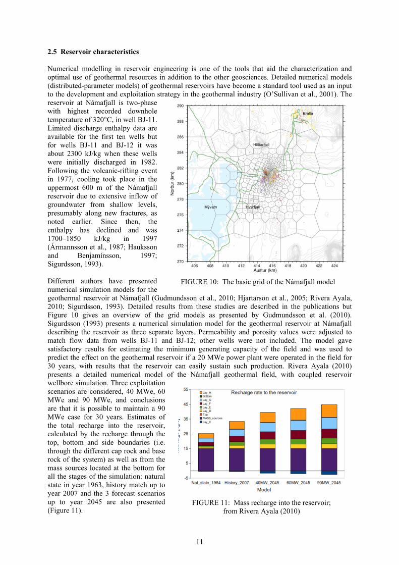
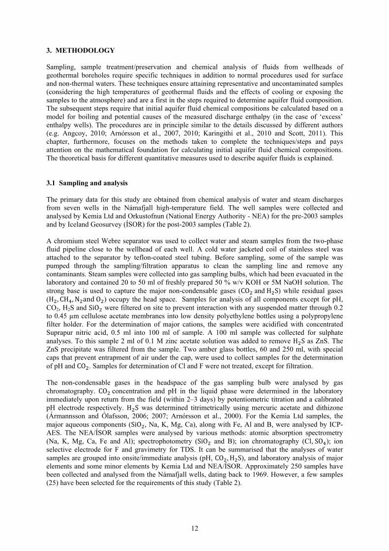
2.5 Reservoir characteristics Numerical modelling in reservoir engineering is one of the tools that aid the characterization and optimal use of geothermal resources in addition to the other geosciences. Detailed numerical models (distributed-parameter models) of geothermal reservoirs have become a standard tool used as an input to the development and exploitation strategy in the geothermal industry (O’Sullivan et al., 2001). The reservoir at Námafjall is two-phase with highest recorded downhole temperature of 320°C, in well BJ-11. Limited discharge enthalpy data are available for the first ten wells but for wells BJ-11 and BJ-12 it was about 2300 kJ/kg when these wells were initially discharged in 1982. Following the volcanic-rifting event in 1977, cooling took place in the uppermost 600 m of the Námafjall reservoir due to extensive inflow of groundwater from shallow levels, presumably along new fractures, as noted earlier. Since then, the enthalpy has declined and was 1700–1850 kJ/kg in 1997 (Ármannsson et al., 1987; Hauksson and Benjamínsson, 1997; Sigurdsson, 1993). Different authors have presented numerical simulation models for the geothermal reservoir at Námafjall (Gudmundsson et al., 2010; Hjartarson et al., 2005; Rivera Ayala, 2010; Sigurdsson, 1993). Detailed results from these studies are described in the publications but Figure 10 gives an overview of the grid models as presented by Gudmundsson et al. (2010). Sigurdsson (1993) presents a numerical simulation model for the geothermal reservoir at Námafjall describing the reservoir as three separate layers. Permeability and porosity values were adjusted to match flow data from wells BJ-11 and BJ-12; other wells were not included. The model gave satisfactory results for estimating the minimum generating capacity of the field and was used to predict the effect on the geothermal reservoir if a 20 MWe power plant were operated in the field for 30 years, with results that the reservoir can easily sustain such production. Rivera Ayala (2010) presents a detailed numerical model of the Námafjall geothermal field, with coupled reservoir wellbore simulation. Three exploitation scenarios are considered, 40 MWe, 60 MWe and 90 MWe, and conclusions are that it is possible to maintain a 90 MWe case for 30 years. Estimates of the total recharge into the reservoir, calculated by the recharge through the top, bottom and side boundaries (i.e. through the different cap rock and base rock of the system) as well as from the mass sources located at the bottom for all the stages of the simulation: natural state in year 1963, history match up to year 2007 and the 3 forecast scenarios up to year 2045 are also presented (Figure 11).
FIGURE 10: The basic grid of the Námafjall model
FIGURE 11: Mass recharge into the reservoir; from Rivera Ayala (2010)
12
3. METHODOLOGY Sampling, sample treatment/preservation and chemical analysis of fluids from wellheads of geothermal boreholes require specific techniques in addition to normal procedures used for surface and non-thermal waters. These techniques ensure attaining representative and uncontaminated samples (considering the high temperatures of geothermal fluids and the effects of cooling or exposing the samples to the atmosphere) and are a first in the steps required to determine aquifer fluid composition. The subsequent steps require that initial aquifer fluid chemical compositions be calculated based on a model for boiling and potential causes of the measured discharge enthalpy (in the case of ‘excess’ enthalpy wells). The procedures are in principle similar to the details discussed by different authors (e.g. Angcoy, 2010; Arnórsson et al., 2007, 2010; Karingithi et al., 2010 and Scott, 2011). This chapter, furthermore, focuses on the methods taken to complete the techniques/steps and pays attention on the mathematical foundation for calculating initial aquifer fluid chemical compositions. The theoretical basis for different quantitative measures used to describe aquifer fluids is explained. 3.1 Sampling and analysis The primary data for this study are obtained from chemical analysis of water and steam discharges from seven wells in the Námafjall high-temperature field. The well samples were collected and analysed by Kemia Ltd and Orkustofnun (National Energy Authority - NEA) for the pre-2003 samples and by Iceland Geosurvey (ÍSOR) for the post-2003 samples (Table 2). A chromium steel Webre separator was used to collect water and steam samples from the two-phase fluid pipeline close to the wellhead of each well. A cold water jacketed coil of stainless steel was attached to the separator by teflon-coated steel tubing. Before sampling, some of the sample was pumped through the sampling/filtration apparatus to clean the sampling line and remove any contaminants. Steam samples were collected into gas sampling bulbs, which had been evacuated in the laboratory and contained 20 to 50 ml of freshly prepared 50 % w/v KOH or 5M NaOH solution. The strong base is used to capture the major non-condensable gases (CO and H S) while residual gases (H , CH , N and O ) occupy the head space. Samples for analysis of all components except for pH, CO2, H2S and SiO were filtered on site to prevent interaction with any suspended matter through 0.2 to 0.45 µm cellulose acetate membranes into low density polyethylene bottles using a polypropylene filter holder. For the determination of major cations, the samples were acidified with concentrated Suprapur nitric acid, 0.5 ml into 100 ml of sample. A 100 ml sample was collected for sulphate analyses. To this sample 2 ml of 0.1 M zinc acetate solution was added to remove H S as ZnS. The ZnS precipitate was filtered from the sample. Two amber glass bottles, 60 and 250 ml, with special caps that prevent entrapment of air under the cap, were used to collect samples for the determination of pH and CO . Samples for determination of Cl and F were not treated, except for filtration. The non-condensable gases in the headspace of the gas sampling bulb were analysed by gas chromatography. CO concentration and pH in the liquid phase were determined in the laboratory immediately upon return from the field (within 2–3 days) by potentiometric titration and a calibrated pH electrode respectively. H S was determined titrimetrically using mercuric acetate and dithizone (Ármannsson and Ólafsson, 2006; 2007; Arnórsson et al., 2000). For the Kemia Ltd samples, the major aqueous components (SiO , Na, K, Mg, Ca), along with Fe, Al and B, were analysed by ICP-AES. The NEA/ÍSOR samples were analysed by various methods: atomic absorption spectrometry (Na, K, Mg, Ca, Fe and Al); spectrophotometry (SiO and B); ion chromatography (Cl, SO ); ion selective electrode for F and gravimetry for TDS. It can be summarised that the analyses of water samples are grouped into onsite/immediate analysis (pH, CO , H S), and laboratory analysis of major elements and some minor elements by Kemia Ltd and NEA/ÍSOR. Approximately 250 samples have been collected and analysed from the Námafjall wells, dating back to 1969. However, a few samples (25) have been selected for the requirements of this study (Table 2).
13
CO
2H
2SB
SiO
2N
aK
Mg
Ca
FC
lSO
4A
lFe
TDS
Gas
(l/k
g)
/ T (2
0o C)
CO
2H
2SH
2O
2C
H4
N2
CO
2H
2SpH
/°CC
O2
H2S
Na
4036
Jun-
9998
3a3.
709.
55/2
1.3
35.2
109.
50.
9554
718
520
.00.
010
4.76
0.79
41.3
37.0
0.69
0.08
092
00.
9787
.41.
34.
96.
324
0495
910
14M
ay-8
610
19a
5.20
9.44
/26.
148
.989
.10.
7547
015
121
.93.
300.
6747
.021
.810
081.
5032
.413
.837
.410
.06.
34.
44/2
6.42
342
20.
4810
12M
ar-7
910
33a
8.10
9.12
/23.
069
.212
5.0
515
149
23.8
2.54
0.72
23.6
22.9
1097
3.80
32.9
13.3
46.7
0.3
6.8
4.30
/23.
541
566
0.78
4034
*Ju
n-07
1014
a11
.89.
03/2
3.2
37.1
122.
70.
7543
213
917
.90.
090
2.60
0.64
37.1
39.0
0.83
0.00
883
71.
7590
.50.
13.
95.
621
8012
7340
08*
Apr
-04
1060
a13
.58.
96/2
1.9
29.7
126.
60.
7754
513
818
.00.
010
2.44
0.72
36.4
71.0
0.92
0.00
697
91.
7291
.10.
33.
55.
124
3113
2940
33M
ay-0
316
2019
.08.
50/2
0.2
2.1
115.
42.
1060
410
117
.00.
010
0.50
0.69
38.4
24.0
2.00
0.01
083
41.
4495
.90.
11.
22.
837
5713
7440
59Ju
l-98
1850
23.5
8.10
/25.
031
.495
.12.
6757
611
816
.20.
001
0.39
0.60
37.4
14.0
0.03
084
81.
3797
.10.
20.
91.
827
5112
9840
35Ju
l-97
1850
23.1
7.97
/25.
729
.495
.01.
9356
087
.014
.50.
010
0.26
0.76
37.7
13.9
0.01
080
01.
4496
.90.
20.
82.
125
5413
2640
13M
ay-9
518
6714
.58.
83/2
5.8
24.2
86.3
1.22
563
121
18.5
0.03
00.
270.
8839
.218
.00.
010
894
1.12
96.1
0.2
0.8
2.9
1779
1213
4024
May
-94
1867
19.0
8.42
/20.
828
.689
.556
694
.014
.80.
050
0.53
0.93
41.8
10.0
0.01
080
81.
3194
.60.
30.
74.
418
9612
9540
22M
ay-9
319
8119
.98.
19/2
0.7
82.9
51.3
542
115
15.4
0.05
00.
260.
7737
.818
.00.
010
1056
1.50
97.8
0.2
1.3
0.7
1453
1538
1034
Jun-
8522
9314
.78.
72/2
4.5
20.6
114.
15.
1742
610
416
.40.
450.
7722
.89.
91.
4283
61.
0620
.121
.257
.30.
31.
14.
35/2
4.26
073
30.
3210
22M
ay-8
323
0916
.28.
60/2
1.0
19.6
110.
444
097
.415
.10.
008
0.68
0.69
22.8
11.2
660
1.96
16.7
19.8
62.3
0.2
1.0
4.51
/21.
217
905
1.70
1050
Aug
-81
2355
18.0
8.20
/26.
050
.795
.941
292
.414
.90.
004
0.79
0.65
25.0
11.3
820
1.20
21.1
25.4
52.2
1.1
0.3
4.45
/26.
130
738
2.36
1024
Jun-
8023
5511
.08.
75/2
5.0
24.7
78.6
436
95.0
13.9
0.01
60.
930.
5629
.810
.563
61.
0416
.315
.866
.70.
21.
05.
52/2
5.25
736
454
.040
34M
ay-0
318
1316
.08.
19/2
0.2
7.4
109.
63.
4058
212
722
.00.
010
0.60
0.52
100
13.0
0.60
0.01
088
32.
0097
.80.
20.
81.
238
6419
2540
13M
ay-9
021
2717
.87.
6/26
.034
.514
3.0
572
153
21.2
0.04
30.
510.
6279
.125
.012
162.
2295
.30.
81.
12.
825
7016
6340
10M
ay-8
921
3815
.97.
89/2
0.0
53.0
133.
062
314
421
.20.
180
0.47
0.62
36.8
31.0
0.10
010
212.
1496
.60.
60.
72.
120
3417
7410
33Se
p-87
2203
19.6
8.43
/19.
042
.013
5.0
521
147
20.2
0.06
00.
650.
5866
.83.
010
252.
1725
.418
.854
.60.
21.
04.
42/1
9.34
468
70.
2510
21M
ay-8
324
0217
.09.
43/2
5.0
25.8
98.5
535
135
18.2
0.00
50.
220.
8824
.57.
210
321.
9223
.318
.357
.20.
10.
21.
04.
42/2
1.34
877
10.
9010
38Ju
l-81
2380
20.2
8.32
/24.
030
.018
9.0
478
135
18.5
0.00
30.
140.
8110
.84.
091
12.
9618
.820
.060
.20.
10.
84.
38/2
4.54
451
20.
3510
05M
ar-8
123
2118
.08.
5/22
.027
.914
7.0
552
143
18.2
0.01
80.
380.
8748
.26.
299
00.
3818
.116
.864
.20.
10.
84.
16/2
2.17
576
80.
32
BJ-1
305
51*
Sep-
0620
2115
.29.
18/2
3.1
5.7
53.3
0.21
766
114
22.4
0.00
51.
110.
8078
.825
.92.
180.
019
1170
0.52
91.4
0.2
8.2
560
526
BJ-1
403
11*
Jul-0
818
0715
.99.
05/2
1.7
4.2
104.
01.
0077
624
049
.60.
004
1.15
1.03
260
19.5
1.53
0.00
916
100.
9883
.91.
314
.657
013
30
BJ-1
503
43*
Aug
-08
1169
a10
.08.
88/1
9.6
161
1.2
0.80
426
160
17.5
0.00
11.
291.
3950
.626
.91.
360.
003
868
2.58
87.3
3.6
9.0
1765
2320
Wel
l N
o.Sa
mpl
e N
o.D
ate
hd,t
(kJ/
kg)
SPb
(bar
-g)
a liq
uid e
ntha
lpy
well
sam
ples
,b Sam
pling
pre
ssur
e (b
ar-g
), hd,
t disc
harg
e en
thal
py (k
J/kg)
, *s
ampl
ed a
nd a
nalys
ed b
y IS
OR,
oth
erw
ise b
y K
emia
Ltd
and
NEA
.
BN-0
9
BJ-1
1
BJ-1
2
pH/°C
Liqu
id c
ompo
nent
s (m
g/kg
)G
as (v
olum
e %
)To
tal
stea
m
(mg/
kg)
Con
dens
ate
(mg/
kg)
BN-0
4
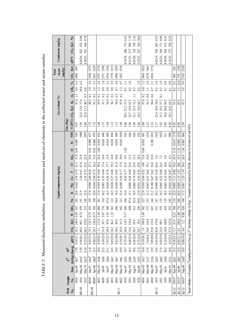
TA
BL
E2:
Mea
sure
ddi
scha
rge
enth
alpi
es,s
ampl
ing
pres
sure
san
dan
alys
isof
elem
ents
inth
eco
llec
ted
wat
eran
dst
eam
sam
ples
14
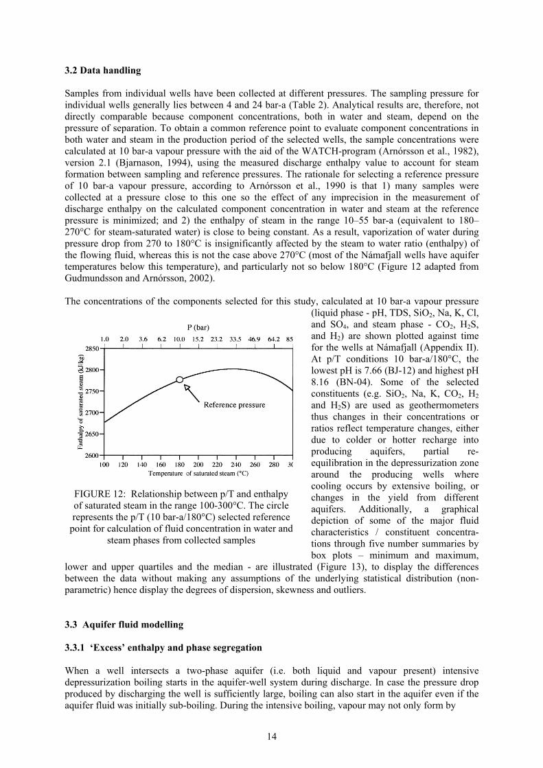
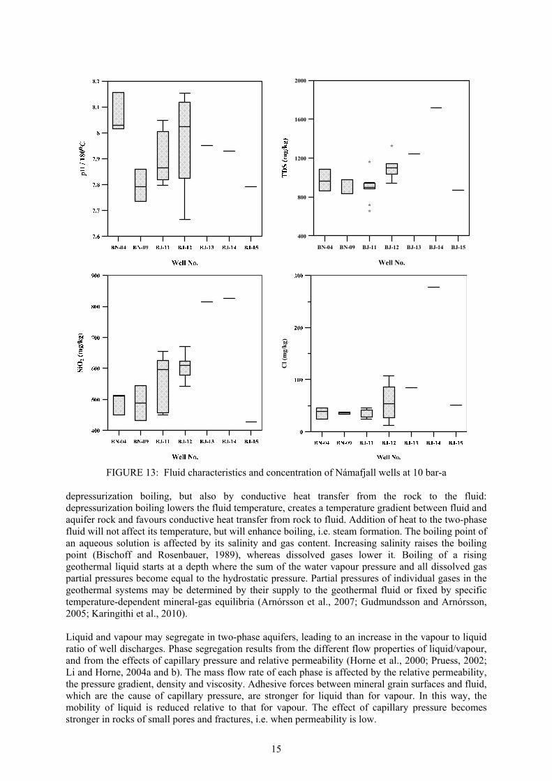
3.2 Data handling Samples from individual wells have been collected at different pressures. The sampling pressure for individual wells generally lies between 4 and 24 bar-a (Table 2). Analytical results are, therefore, not directly comparable because component concentrations, both in water and steam, depend on the pressure of separation. To obtain a common reference point to evaluate component concentrations in both water and steam in the production period of the selected wells, the sample concentrations were calculated at 10 bar-a vapour pressure with the aid of the WATCH-program (Arnórsson et al., 1982), version 2.1 (Bjarnason, 1994), using the measured discharge enthalpy value to account for steam formation between sampling and reference pressures. The rationale for selecting a reference pressure of 10 bar-a vapour pressure, according to Arnórsson et al., 1990 is that 1) many samples were collected at a pressure close to this one so the effect of any imprecision in the measurement of discharge enthalpy on the calculated component concentration in water and steam at the reference pressure is minimized; and 2) the enthalpy of steam in the range 10–55 bar-a (equivalent to 180–270°C for steam-saturated water) is close to being constant. As a result, vaporization of water during pressure drop from 270 to 180°C is insignificantly affected by the steam to water ratio (enthalpy) of the flowing fluid, whereas this is not the case above 270°C (most of the Námafjall wells have aquifer temperatures below this temperature), and particularly not so below 180°C (Figure 12 adapted from Gudmundsson and Arnórsson, 2002). The concentrations of the components selected for this study, calculated at 10 bar-a vapour pressure
(liquid phase - pH, TDS, SiO2, Na, K, Cl, and SO4, and steam phase - CO2, H2S, and H2) are shown plotted against time for the wells at Námafjall (Appendix II). At p/T conditions 10 bar-a/180°C, the lowest pH is 7.66 (BJ-12) and highest pH 8.16 (BN-04). Some of the selected constituents (e.g. SiO2, Na, K, CO2, H2 and H2S) are used as geothermometers thus changes in their concentrations or ratios reflect temperature changes, either due to colder or hotter recharge into producing aquifers, partial re-equilibration in the depressurization zone around the producing wells where cooling occurs by extensive boiling, or changes in the yield from different aquifers. Additionally, a graphical depiction of some of the major fluid characteristics / constituent concentra-tions through five number summaries by box plots – minimum and maximum,
lower and upper quartiles and the median - are illustrated (Figure 13), to display the differences between the data without making any assumptions of the underlying statistical distribution (non-parametric) hence display the degrees of dispersion, skewness and outliers. 3.3 Aquifer fluid modelling 3.3.1 ‘Excess’ enthalpy and phase segregation When a well intersects a two-phase aquifer (i.e. both liquid and vapour present) intensive depressurization boiling starts in the aquifer-well system during discharge. In case the pressure drop produced by discharging the well is sufficiently large, boiling can also start in the aquifer even if the aquifer fluid was initially sub-boiling. During the intensive boiling, vapour may not only form by
FIGURE 12: Relationship between p/T and enthalpy of saturated steam in the range 100-300°C. The circle represents the p/T (10 bar-a/180°C) selected reference
point for calculation of fluid concentration in water and steam phases from collected samples
15
depressurization boiling, but also by conductive heat transfer from the rock to the fluid: depressurization boiling lowers the fluid temperature, creates a temperature gradient between fluid and aquifer rock and favours conductive heat transfer from rock to fluid. Addition of heat to the two-phase fluid will not affect its temperature, but will enhance boiling, i.e. steam formation. The boiling point of an aqueous solution is affected by its salinity and gas content. Increasing salinity raises the boiling point (Bischoff and Rosenbauer, 1989), whereas dissolved gases lower it. Boiling of a rising geothermal liquid starts at a depth where the sum of the water vapour pressure and all dissolved gas partial pressures become equal to the hydrostatic pressure. Partial pressures of individual gases in the geothermal systems may be determined by their supply to the geothermal fluid or fixed by specific temperature-dependent mineral-gas equilibria (Arnórsson et al., 2007; Gudmundsson and Arnórsson, 2005; Karingithi et al., 2010). Liquid and vapour may segregate in two-phase aquifers, leading to an increase in the vapour to liquid ratio of well discharges. Phase segregation results from the different flow properties of liquid/vapour, and from the effects of capillary pressure and relative permeability (Horne et al., 2000; Pruess, 2002; Li and Horne, 2004a and b). The mass flow rate of each phase is affected by the relative permeability, the pressure gradient, density and viscosity. Adhesive forces between mineral grain surfaces and fluid, which are the cause of capillary pressure, are stronger for liquid than for vapour. In this way, the mobility of liquid is reduced relative to that for vapour. The effect of capillary pressure becomes stronger in rocks of small pores and fractures, i.e. when permeability is low.
FIGURE 13: Fluid characteristics and concentration of Námafjall wells at 10 bar-a
400
800
1200
1600
2000
BN-04 BN-09 BJ-11 BJ-12 BJ-13 BJ-14 BJ-15
Well No.
Cl(
mg/
kg)

16
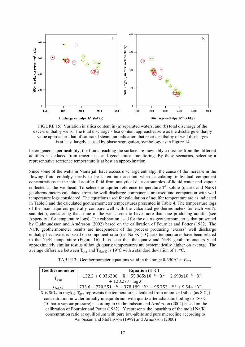
Due to boiling and phase segregation in two-phase aquifers, the discharge enthalpy of wells producing from liquid-dominated geothermal reservoirs is often higher than the enthalpy of the initial aquifer fluid, and it is not uncommon that wells drilled into such systems discharge steam only. Wells with discharge enthalpies higher than that of steam-saturated water at the aquifer temperature have been referred to as “excess enthalpy wells” (Angcoy, 2010; Arnórsson et al., 2007; 2010; Karingithi et al., 2010; Scott, 2011). Some of the excess enthalpy may be due to the presence of vapour in the initial aquifer fluid. However, the effects of conductive heat transfer, phase segregation, or both, generally seem to be more important. To calculate the chemical composition of the initial aquifer liquid and vapour, the relative contributions of the different processes to the excess discharge enthalpy and the initial vapour fraction of the aquifer fluid need to be evaluated. Wells BN-04, BN-09 and BJ-15 in Námafjall field are considered to have liquid enthalpy (Table 2 and Figure 14), i.e. the enthalpy of the discharge is the same (within the limit of measurement error) to that of steam saturated liquid at the aquifer temperature, thus for liquid enthalpy wells, it is a reasonable assumption to take the total well discharge composition to represent the initial aquifer fluid. The other wells (BJ-11, BJ-12, BJ-13 and BJ-14) display variable degrees of ‘excess’ enthalpy although the discharge enthalpy has decreased with time in the wells for which data are available for more than 15 years (Figure 14). For excess enthalpy wells, a model needs to be selected that explains the cause of the elevated well enthalpy by considering the effects of depressurization boiling, possible phase segregation in the depressurization zones around wells, conductive heat transfer from the aquifer rock to the flowing fluid that enhances boiling as well as loss of gaseous steam from the fluid flowing into wells, likely during horizontal flow. Glover et al. (1981) used the chemistry of well discharges in a simple way to distinguish between excess well enthalpy caused by phase segregation from that caused by conductive heat transfer from aquifer rock to fluid. For phase segregation, the concentration of a conservative component that only occupies the liquid is expected to decrease in the total discharge with increasing discharge enthalpy and approach zero as the discharge enthalpy approaches that of saturated steam. For many wet-steam wells, discharge enthalpy may not vary sufficiently with time to make the method of Glover et al. (1981) applicable. In a specific well-field, one may use many wells with a range of discharge enthalpies to determine whether conductive heat transfer or phase segregation dominates the excess enthalpy. If conservative components like Cl vary much across the well field, they may not be a good choice, but if aquifer temperatures are about constant, SiO2 is useful because its concentration is determined almost solely by temperature through its equilibrium with quartz (Figure 15). The observed correlation for SiO2 in the total discharge for the excess enthalpy wells at Námafjall suggests that phase segregation in the producing aquifers is largely the cause of excess well discharge enthalpy. 3.3.2 Aquifer fluid temperature Many chemical and isotopic geothermometers are used to estimate the aquifer temperatures beyond the zone of secondary processes like boiling, cooling and mixing on the basic assumptions that the sampled fluids are representative of the undisturbed aquifers where local equilibrium conditions are achieved. Actual downhole measurements may or may not agree with geothermometers. For fields of
FIGURE 14: Discharge enthalpy of wells in Námafjall field; numbers in the symbols indicate the sample
17
heterogeneous permeability, the fluids reaching the surface are inevitably a mixture from the different aquifers as deduced from tracer tests and geochemical monitoring. By these scenarios, selecting a representative reference temperature is at best an approximation. Since some of the wells in Námafjall have excess discharge enthalpy, the cause of the increase in the flowing fluid enthalpy needs to be taken into account when calculating individual component concentrations in the initial aquifer fluid from analytical data on samples of liquid water and vapour collected at the wellhead. To select the aquifer reference temperature, T , solute (quartz and Na/K) geothermometers calculated from the well discharge components are used and comparison with well temperature logs considered. The equations used for calculation of aquifer temperature are as indicated in Table 3 and the calculated geothermometer temperatures presented in Table 4. The temperature logs of the main aquifers generally compare well with the calculated geothermometers for each well’s sample(s), considering that some of the wells seem to have more than one producing aquifer (see Appendix I for temperature logs). The calibration used for the quartz geothermometer is that presented by Gudmundsson and Arnórsson (2002) based on the calibration of Fournier and Potter (1982). The Na/K geothermometer results are independent of the process producing ‘excess’ well discharge enthalpy because it is based on component ratio (i.e. Na+/K+). Quartz temperatures have been related to the Na/K temperature (Figure 16). It is seen that the quartz and Na/K geothermometers yield approximately similar results although quartz temperatures are systematically higher on average. The average difference between T and T ⁄ is 19°C with a standard deviation of 11°C.
FIGURE 15: Variation in silica content in (a) separated waters, and (b) total discharge of the
excess enthalpy wells. The total discharge silica content approaches zero as the discharge enthalpy value approaches that of saturated steam: an indication that excess enthalpy of well discharges
is at least largely caused by phase segregation, symbology as in Figure 14
a.
1500 1800 2100 2400 2700 3000
Discharge enthalpy, hd,t (kJ/kg)
0
150
300
450
600
4033
40594035
40134024
4022
1034102210501024
4034
40134010
1033
10211038
1005
0551
0311
b.
TABLE 3: Geothermometer equations valid in the range 0-350°C at .
Geothermometer Equation (T°C)
−132.2 + 0.036206 ∙ X + 55.865x10 ∙ X − 2.699x10 ∙ X+ 128.277 ∙ log ⁄ 733.6 − 770.551 ∙ Y + 378.189 ∙ Y − 95.753 ∙ Y + 9.544 ∙ Y X is SiO in mg/kg. T represents the temperature calculated from unionized silica (as SiO )
concentration in water initially in equilibrium with quartz after adiabatic boiling to 180°C (10 bar-a vapour pressure) according to Gudmundsson and Arnórsson (2002) based on the calibration of Fournier and Potter (1982). Y represents the logarithm of the molal Na/K concentration ratio at equilibrium with pure low-albite and pure microcline according to
Arnórsson and Stefánsson (1999) and Arnórsson (2000)
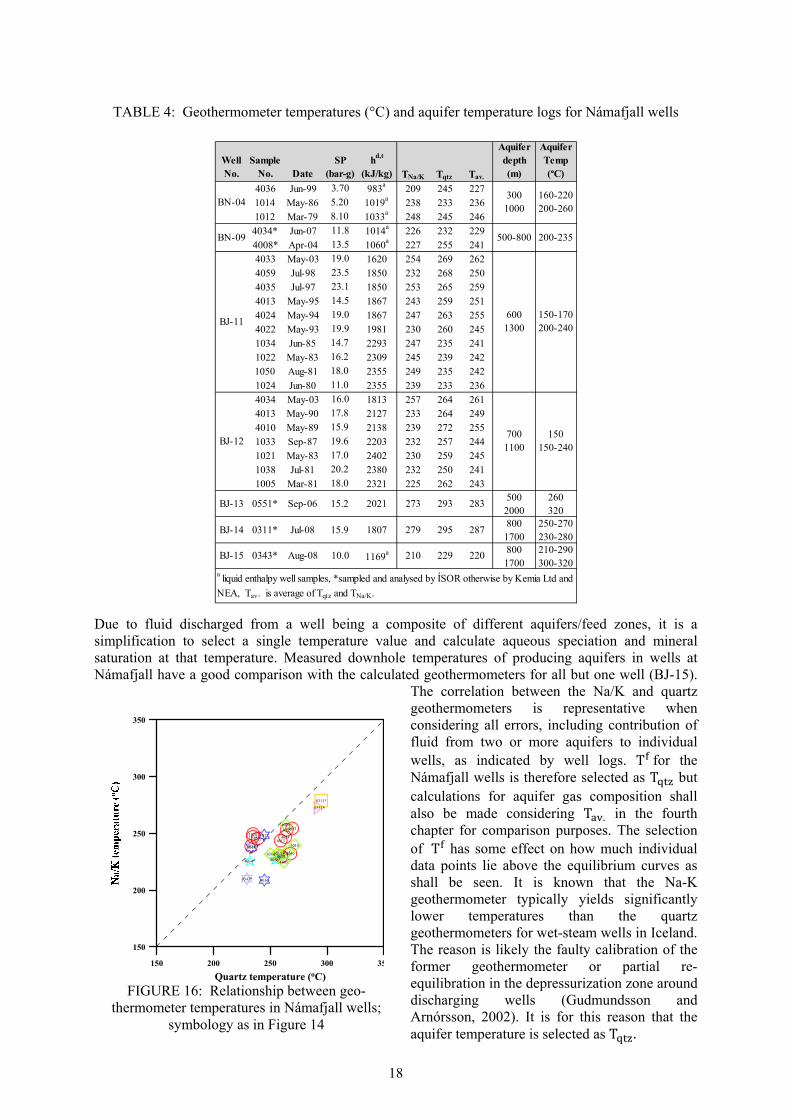
18
Due to fluid discharged from a well being a composite of different aquifers/feed zones, it is a simplification to select a single temperature value and calculate aqueous speciation and mineral saturation at that temperature. Measured downhole temperatures of producing aquifers in wells at Námafjall have a good comparison with the calculated geothermometers for all but one well (BJ-15).
The correlation between the Na/K and quartz geothermometers is representative when considering all errors, including contribution of fluid from two or more aquifers to individual wells, as indicated by well logs. T for the Námafjall wells is therefore selected as T but calculations for aquifer gas composition shall also be made considering T . in the fourth chapter for comparison purposes. The selection of T has some effect on how much individual data points lie above the equilibrium curves as shall be seen. It is known that the Na-K geothermometer typically yields significantly lower temperatures than the quartz geothermometers for wet-steam wells in Iceland. The reason is likely the faulty calibration of the former geothermometer or partial re-equilibration in the depressurization zone around discharging wells (Gudmundsson and Arnórsson, 2002). It is for this reason that the aquifer temperature is selected as T .
TABLE 4: Geothermometer temperatures (°C) and aquifer temperature logs for Námafjall wells
Well No.
Sample No. Date
SP (bar-g)
hd,t
(kJ/kg) TNa/K Tqtz Tav.
Aquifer depth (m)
Aquifer Temp (°C)
4036 Jun-99 3.70 983a 209 245 2271014 May-86 5.20 1019a 238 233 2361012 Mar-79 8.10 1033a 248 245 2464034* Jun-07 11.8 1014a 226 232 2294008* Apr-04 13.5 1060a 227 255 2414033 May-03 19.0 1620 254 269 2624059 Jul-98 23.5 1850 232 268 2504035 Jul-97 23.1 1850 253 265 2594013 May-95 14.5 1867 243 259 2514024 May-94 19.0 1867 247 263 2554022 May-93 19.9 1981 230 260 2451034 Jun-85 14.7 2293 247 235 2411022 May-83 16.2 2309 245 239 2421050 Aug-81 18.0 2355 249 235 2421024 Jun-80 11.0 2355 239 233 2364034 May-03 16.0 1813 257 264 2614013 May-90 17.8 2127 233 264 2494010 May-89 15.9 2138 239 272 2551033 Sep-87 19.6 2203 232 257 2441021 May-83 17.0 2402 230 259 2451038 Jul-81 20.2 2380 232 250 2411005 Mar-81 18.0 2321 225 262 243
BJ-13 0551* Sep-06 15.2 2021 273 293 283500 2000
260 320
BJ-14 0311* Jul-08 15.9 1807 279 295 287800 1700
250-270 230-280
BJ-15 0343* Aug-08 10.0 1169a 210 229 220800 1700
210-290 300-320
BN-09
300 1000
500-800
600 1300
700 1100
BN-04
BJ-11
160-220 200-260
200-235
150-170 200-240
150 150-240
a liquid enthalpy well samples, *sampled and analysed by ÍSOR otherwise by Kemia Ltd and
NEA, Tav. is average of Tqtz and TNa/K.
BJ-12
FIGURE 16: Relationship between geo-thermometer temperatures in Námafjall wells;
symbology as in Figure 14
150 200 250 300 35
Quartz temperature (oC)
150
200
250
300
350
4036
1014
1012
4034* 4008*
4033
4059
4035
40134024
4022
103410221050
1024
4034
4013
4010
103310211038
1005
0551*
0311*
0343*
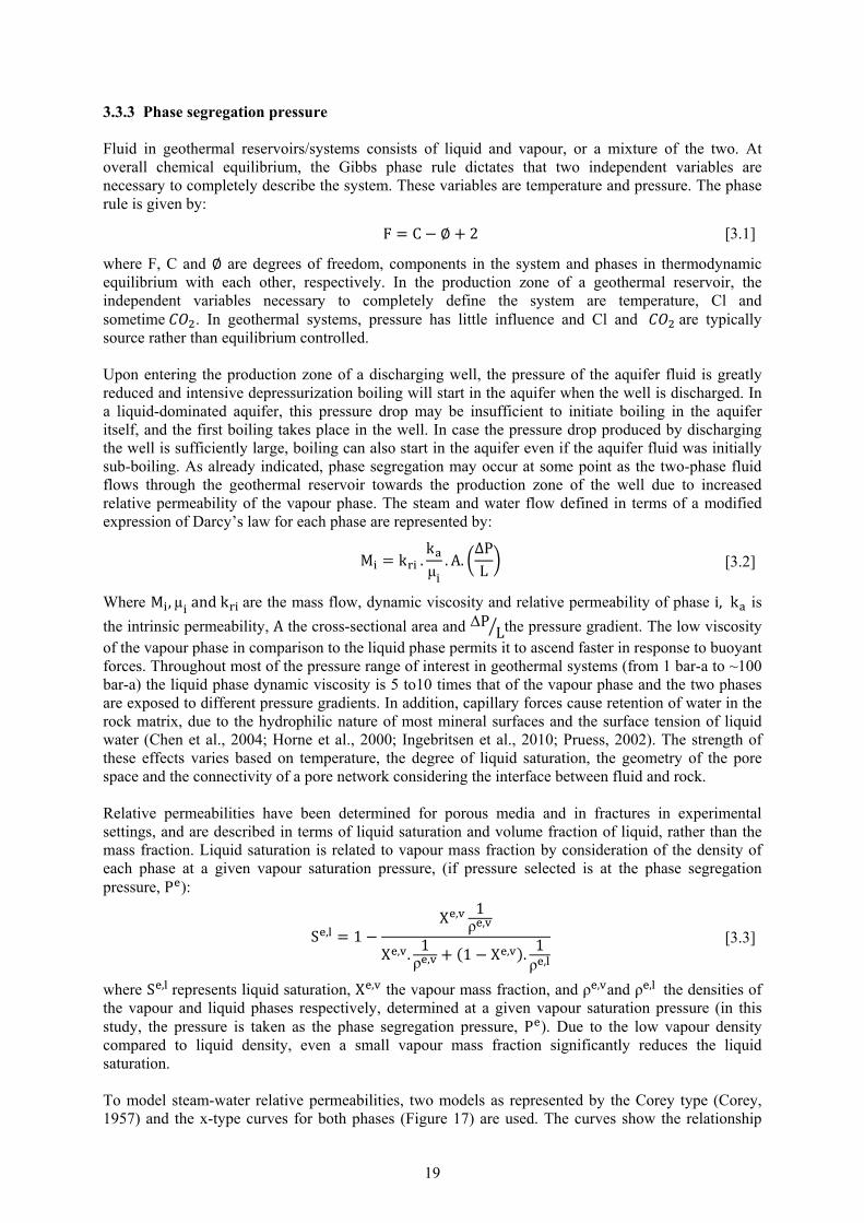
19
3.3.3 Phase segregation pressure Fluid in geothermal reservoirs/systems consists of liquid and vapour, or a mixture of the two. At overall chemical equilibrium, the Gibbs phase rule dictates that two independent variables are necessary to completely describe the system. These variables are temperature and pressure. The phase rule is given by:
F = C − ∅ + 2 [3.1]
where F, C and ∅ are degrees of freedom, components in the system and phases in thermodynamic equilibrium with each other, respectively. In the production zone of a geothermal reservoir, the independent variables necessary to completely define the system are temperature, Cl and sometime . In geothermal systems, pressure has little influence and Cl and are typically source rather than equilibrium controlled. Upon entering the production zone of a discharging well, the pressure of the aquifer fluid is greatly reduced and intensive depressurization boiling will start in the aquifer when the well is discharged. In a liquid-dominated aquifer, this pressure drop may be insufficient to initiate boiling in the aquifer itself, and the first boiling takes place in the well. In case the pressure drop produced by discharging the well is sufficiently large, boiling can also start in the aquifer even if the aquifer fluid was initially sub-boiling. As already indicated, phase segregation may occur at some point as the two-phase fluid flows through the geothermal reservoir towards the production zone of the well due to increased relative permeability of the vapour phase. The steam and water flow defined in terms of a modified expression of Darcy’s law for each phase are represented by:
M = k . kμ
. A. ∆PL [3.2]
Where M , µ and k are the mass flow, dynamic viscosity and relative permeability of phase i, k is
the intrinsic permeability, A the cross-sectional area and ΔP Lthe pressure gradient. The low viscosity of the vapour phase in comparison to the liquid phase permits it to ascend faster in response to buoyant forces. Throughout most of the pressure range of interest in geothermal systems (from 1 bar-a to ~100 bar-a) the liquid phase dynamic viscosity is 5 to10 times that of the vapour phase and the two phases are exposed to different pressure gradients. In addition, capillary forces cause retention of water in the rock matrix, due to the hydrophilic nature of most mineral surfaces and the surface tension of liquid water (Chen et al., 2004; Horne et al., 2000; Ingebritsen et al., 2010; Pruess, 2002). The strength of these effects varies based on temperature, the degree of liquid saturation, the geometry of the pore space and the connectivity of a pore network considering the interface between fluid and rock. Relative permeabilities have been determined for porous media and in fractures in experimental settings, and are described in terms of liquid saturation and volume fraction of liquid, rather than the mass fraction. Liquid saturation is related to vapour mass fraction by consideration of the density of each phase at a given vapour saturation pressure, (if pressure selected is at the phase segregation pressure, P ):
S , = 1 − X , 1ρ ,X , . 1
ρ , + (1 − X , ). 1ρ , [3.3]
where S , represents liquid saturation, X , the vapour mass fraction, and ρ , and ρ , the densities of the vapour and liquid phases respectively, determined at a given vapour saturation pressure (in this study, the pressure is taken as the phase segregation pressure, P ). Due to the low vapour density compared to liquid density, even a small vapour mass fraction significantly reduces the liquid saturation. To model steam-water relative permeabilities, two models as represented by the Corey type (Corey, 1957) and the x-type curves for both phases (Figure 17) are used. The curves show the relationship
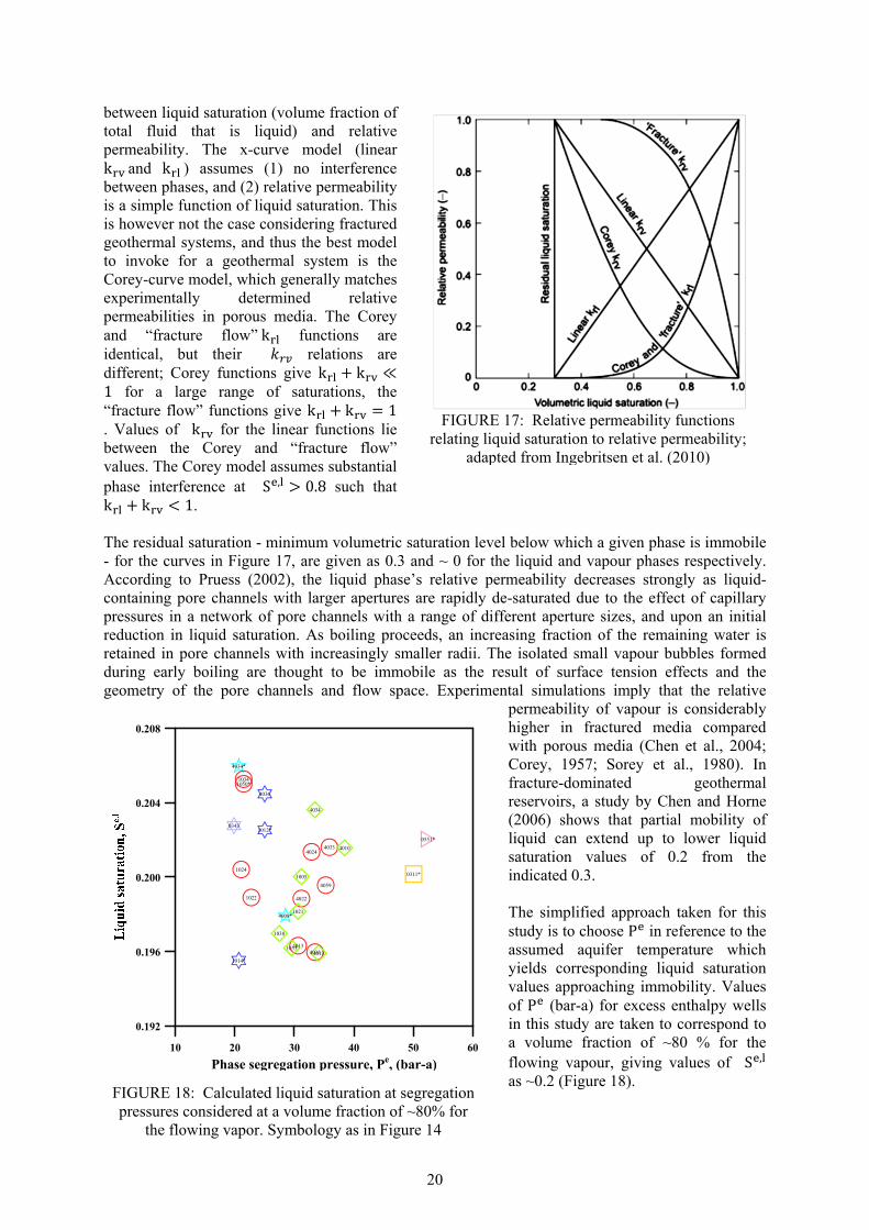
20
between liquid saturation (volume fraction of total fluid that is liquid) and relative permeability. The x-curve model (linear k and k ) assumes (1) no interference between phases, and (2) relative permeability is a simple function of liquid saturation. This is however not the case considering fractured geothermal systems, and thus the best model to invoke for a geothermal system is the Corey-curve model, which generally matches experimentally determined relative permeabilities in porous media. The Corey and “fracture flow” k functions are identical, but their relations are different; Corey functions give k + k ≪1 for a large range of saturations, the “fracture flow” functions give k + k = 1 . Values of k for the linear functions lie between the Corey and “fracture flow” values. The Corey model assumes substantial phase interference at S , 0.8 such that k + k 1. The residual saturation - minimum volumetric saturation level below which a given phase is immobile - for the curves in Figure 17, are given as 0.3 and ~ 0 for the liquid and vapour phases respectively. According to Pruess (2002), the liquid phase’s relative permeability decreases strongly as liquid-containing pore channels with larger apertures are rapidly de-saturated due to the effect of capillary pressures in a network of pore channels with a range of different aperture sizes, and upon an initial reduction in liquid saturation. As boiling proceeds, an increasing fraction of the remaining water is retained in pore channels with increasingly smaller radii. The isolated small vapour bubbles formed during early boiling are thought to be immobile as the result of surface tension effects and the geometry of the pore channels and flow space. Experimental simulations imply that the relative
permeability of vapour is considerably higher in fractured media compared with porous media (Chen et al., 2004; Corey, 1957; Sorey et al., 1980). In fracture-dominated geothermal reservoirs, a study by Chen and Horne (2006) shows that partial mobility of liquid can extend up to lower liquid saturation values of 0.2 from the indicated 0.3. The simplified approach taken for this study is to choose P in reference to the assumed aquifer temperature which yields corresponding liquid saturation values approaching immobility. Values of P (bar-a) for excess enthalpy wells in this study are taken to correspond to a volume fraction of ~80 % for the flowing vapour, giving values of S , as ~0.2 (Figure 18).
FIGURE 18: Calculated liquid saturation at segregation pressures considered at a volume fraction of ~80% for
the flowing vapor. Symbology as in Figure 14
10 20 30 40 50 60
Phase segregation pressure, Pe, (bar-a)
0.192
0.196
0.200
0.204
0.208
4036
1014*
1012*
4034*
4008*
4033
4059
40354013
4024
4022
1034
1022
1050*
1024
4034
4013
4010
1033
1021
1038
1005
0551*
0311*
0343
FIGURE 17: Relative permeability functions
relating liquid saturation to relative permeability; adapted from Ingebritsen et al. (2010)
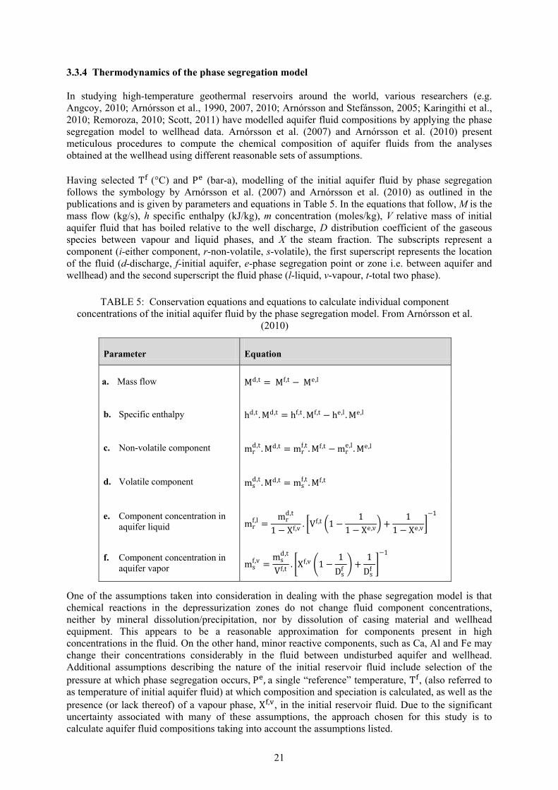
21
3.3.4 Thermodynamics of the phase segregation model In studying high-temperature geothermal reservoirs around the world, various researchers (e.g. Angcoy, 2010; Arnórsson et al., 1990, 2007, 2010; Arnórsson and Stefánsson, 2005; Karingithi et al., 2010; Remoroza, 2010; Scott, 2011) have modelled aquifer fluid compositions by applying the phase segregation model to wellhead data. Arnórsson et al. (2007) and Arnórsson et al. (2010) present meticulous procedures to compute the chemical composition of aquifer fluids from the analyses obtained at the wellhead using different reasonable sets of assumptions. Having selected T (°C) and P (bar-a), modelling of the initial aquifer fluid by phase segregation follows the symbology by Arnórsson et al. (2007) and Arnórsson et al. (2010) as outlined in the publications and is given by parameters and equations in Table 5. In the equations that follow, M is the mass flow (kg/s), h specific enthalpy (kJ/kg), m concentration (moles/kg), V relative mass of initial aquifer fluid that has boiled relative to the well discharge, D distribution coefficient of the gaseous species between vapour and liquid phases, and X the steam fraction. The subscripts represent a component (i-either component, r-non-volatile, s-volatile), the first superscript represents the location of the fluid (d-discharge, f-initial aquifer, e-phase segregation point or zone i.e. between aquifer and wellhead) and the second superscript the fluid phase (l-liquid, v-vapour, t-total two phase).
One of the assumptions taken into consideration in dealing with the phase segregation model is that chemical reactions in the depressurization zones do not change fluid component concentrations, neither by mineral dissolution/precipitation, nor by dissolution of casing material and wellhead equipment. This appears to be a reasonable approximation for components present in high concentrations in the fluid. On the other hand, minor reactive components, such as Ca, Al and Fe may change their concentrations considerably in the fluid between undisturbed aquifer and wellhead. Additional assumptions describing the nature of the initial reservoir fluid include selection of the pressure at which phase segregation occurs, P , a single “reference” temperature, T , (also referred to as temperature of initial aquifer fluid) at which composition and speciation is calculated, as well as the presence (or lack thereof) of a vapour phase, X , , in the initial reservoir fluid. Due to the significant uncertainty associated with many of these assumptions, the approach chosen for this study is to calculate aquifer fluid compositions taking into account the assumptions listed.
TABLE 5: Conservation equations and equations to calculate individual component concentrations of the initial aquifer fluid by the phase segregation model. From Arnórsson et al.
(2010)
Parameter Equation
a. Mass flow
Md,t = Mf,t − Me,l
b. Specific enthalpy
hd,t . Md,t = hf,t . Mf,t − he,l . Me,l
c. Non-volatile component
mrd,t . Md,t = mrf,t . Mf,t − mre,l . Me,l
d. Volatile component
msd,t . Md,t = msf,t . Mf,t
e. Component concentration in aquifer liquid
mrf,l = mrd,t1 − Xf,v . Vf,t 1 − 11 − Xe,v + 11 − Xe,v −1
f. Component concentration in aquifer vapor msf,v = msd,tVf,t . Xf,v 1 − 1Dsf + 1Dsf
−1
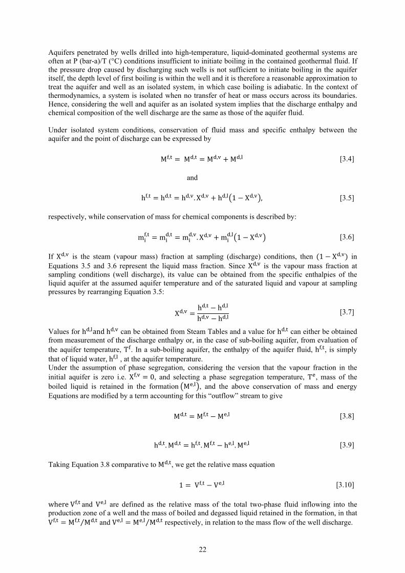
22
Aquifers penetrated by wells drilled into high-temperature, liquid-dominated geothermal systems are often at P (bar-a)/T (°C) conditions insufficient to initiate boiling in the contained geothermal fluid. If the pressure drop caused by discharging such wells is not sufficient to initiate boiling in the aquifer itself, the depth level of first boiling is within the well and it is therefore a reasonable approximation to treat the aquifer and well as an isolated system, in which case boiling is adiabatic. In the context of thermodynamics, a system is isolated when no transfer of heat or mass occurs across its boundaries. Hence, considering the well and aquifer as an isolated system implies that the discharge enthalpy and chemical composition of the well discharge are the same as those of the aquifer fluid. Under isolated system conditions, conservation of fluid mass and specific enthalpy between the aquifer and the point of discharge can be expressed by
and
respectively, while conservation of mass for chemical components is described by:
If X , is the steam (vapour mass) fraction at sampling (discharge) conditions, then (1 − X , ) in Equations 3.5 and 3.6 represent the liquid mass fraction. Since X , is the vapour mass fraction at sampling conditions (well discharge), its value can be obtained from the specific enthalpies of the liquid aquifer at the assumed aquifer temperature and of the saturated liquid and vapour at sampling pressures by rearranging Equation 3.5:
Values for h , and h , can be obtained from Steam Tables and a value for h , can either be obtained from measurement of the discharge enthalpy or, in the case of sub-boiling aquifer, from evaluation of the aquifer temperature, T . In a sub-boiling aquifer, the enthalpy of the aquifer fluid, h , , is simply that of liquid water, h , , at the aquifer temperature. Under the assumption of phase segregation, considering the version that the vapour fraction in the initial aquifer is zero i.e. X , = 0, and selecting a phase segregation temperature, T , mass of the boiled liquid is retained in the formation M , , and the above conservation of mass and energy Equations are modified by a term accounting for this “outflow” stream to give
Taking Equation 3.8 comparative to M , , we get the relative mass equation
where V , and V , are defined as the relative mass of the total two-phase fluid inflowing into the production zone of a well and the mass of boiled and degassed liquid retained in the formation, in that V , = M , M ,⁄ and V , = M , M ,⁄ respectively, in relation to the mass flow of the well discharge.
M , = M , = M , + M , [3.4]
h , = h , = h , . X , + h , 1 − X , , [3.5]
m , = m , = m , . X , + m , 1 − X , [3.6]
X , = h , − h ,h , − h , [3.7]
M , = M , − M , [3.8]
h , . M , = h , . M , − h , . M , [3.9]
1 = V , − V , [3.10]
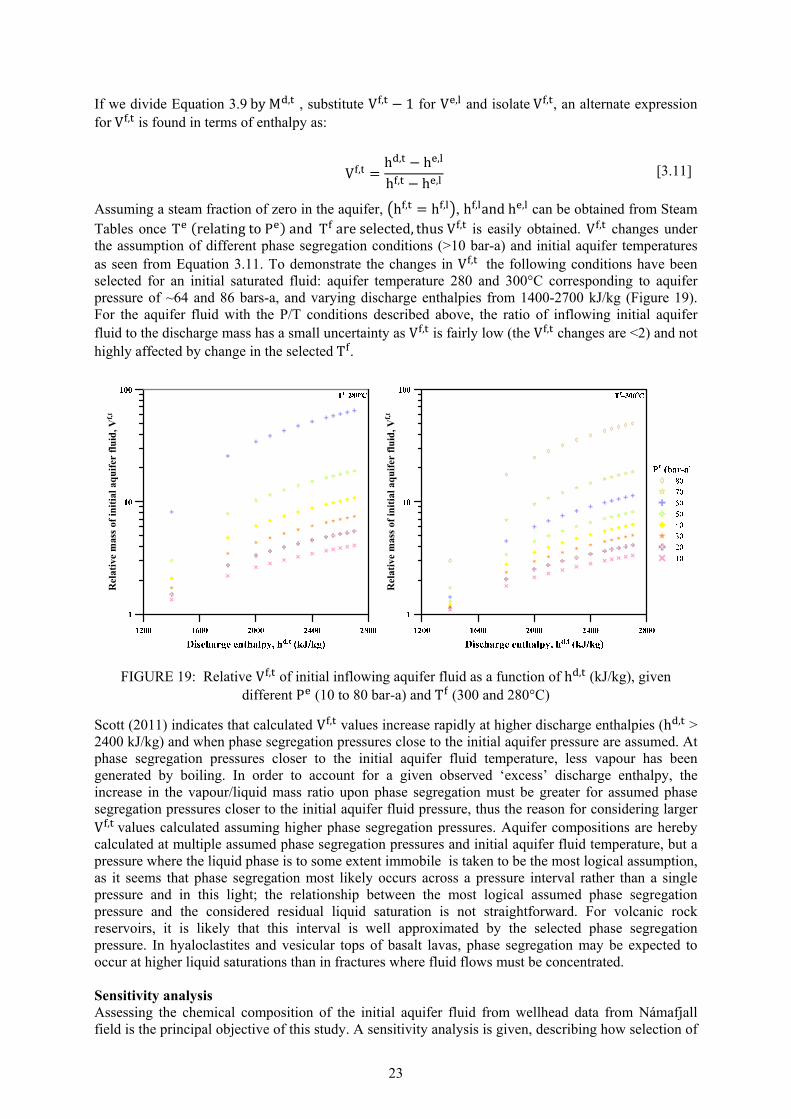
23
If we divide Equation 3.9 by M , , substitute V , − 1 for V , and isolate V , , an alternate expression for V , is found in terms of enthalpy as:
Assuming a steam fraction of zero in the aquifer, h , = h , , h , and h , can be obtained from Steam Tables once T (relating to P ) and T are selected, thus V , is easily obtained. V , changes under the assumption of different phase segregation conditions (>10 bar-a) and initial aquifer temperatures as seen from Equation 3.11. To demonstrate the changes in V , the following conditions have been selected for an initial saturated fluid: aquifer temperature 280 and 300°C corresponding to aquifer pressure of ~64 and 86 bars-a, and varying discharge enthalpies from 1400-2700 kJ/kg (Figure 19). For the aquifer fluid with the P/T conditions described above, the ratio of inflowing initial aquifer fluid to the discharge mass has a small uncertainty as V , is fairly low (the V , changes are <2) and not highly affected by change in the selected T .
Scott (2011) indicates that calculated V , values increase rapidly at higher discharge enthalpies (h , > 2400 kJ/kg) and when phase segregation pressures close to the initial aquifer pressure are assumed. At phase segregation pressures closer to the initial aquifer fluid temperature, less vapour has been generated by boiling. In order to account for a given observed ‘excess’ discharge enthalpy, the increase in the vapour/liquid mass ratio upon phase segregation must be greater for assumed phase segregation pressures closer to the initial aquifer fluid pressure, thus the reason for considering larger V , values calculated assuming higher phase segregation pressures. Aquifer compositions are hereby calculated at multiple assumed phase segregation pressures and initial aquifer fluid temperature, but a pressure where the liquid phase is to some extent immobile is taken to be the most logical assumption, as it seems that phase segregation most likely occurs across a pressure interval rather than a single pressure and in this light; the relationship between the most logical assumed phase segregation pressure and the considered residual liquid saturation is not straightforward. For volcanic rock reservoirs, it is likely that this interval is well approximated by the selected phase segregation pressure. In hyaloclastites and vesicular tops of basalt lavas, phase segregation may be expected to occur at higher liquid saturations than in fractures where fluid flows must be concentrated. Sensitivity analysis Assessing the chemical composition of the initial aquifer fluid from wellhead data from Námafjall field is the principal objective of this study. A sensitivity analysis is given, describing how selection of
V , = h , − h ,h , − h , [3.11]
FIGURE 19: Relative V , of initial inflowing aquifer fluid as a function of h , (kJ/kg), given different P (10 to 80 bar-a) and T (300 and 280°C)
Rel
ativ
em
ass
ofin
itia
laq
uif
erfl
uid
,Vf,
t
Rel
ativ
em
ass
ofin
itia
laq
uif
erfl
uid
,Vf,
t
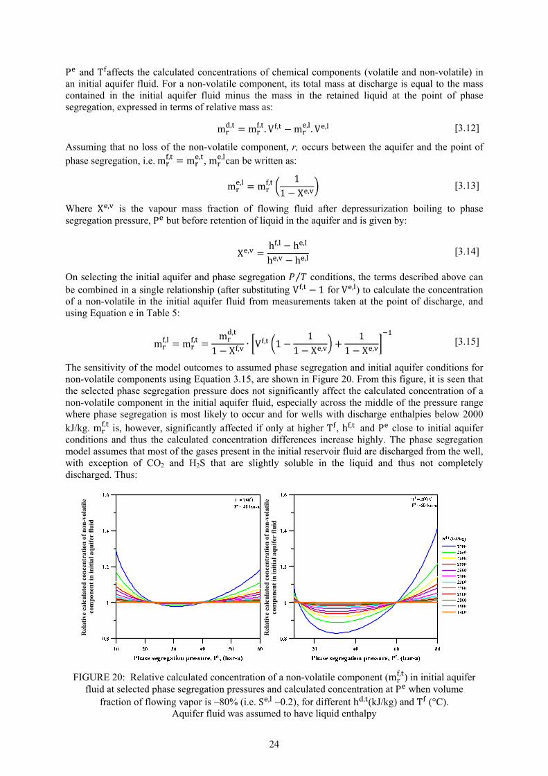
24
P and T affects the calculated concentrations of chemical components (volatile and non-volatile) in an initial aquifer fluid. For a non-volatile component, its total mass at discharge is equal to the mass contained in the initial aquifer fluid minus the mass in the retained liquid at the point of phase segregation, expressed in terms of relative mass as:
Assuming that no loss of the non-volatile component, r, occurs between the aquifer and the point of phase segregation, i.e. m , = m , , m , can be written as:
Where X , is the vapour mass fraction of flowing fluid after depressurization boiling to phase segregation pressure, P but before retention of liquid in the aquifer and is given by:
On selecting the initial aquifer and phase segregation ⁄ conditions, the terms described above can be combined in a single relationship (after substituting V , − 1 for V , ) to calculate the concentration of a non-volatile in the initial aquifer fluid from measurements taken at the point of discharge, and using Equation e in Table 5:
The sensitivity of the model outcomes to assumed phase segregation and initial aquifer conditions for non-volatile components using Equation 3.15, are shown in Figure 20. From this figure, it is seen that the selected phase segregation pressure does not significantly affect the calculated concentration of a non-volatile component in the initial aquifer fluid, especially across the middle of the pressure range where phase segregation is most likely to occur and for wells with discharge enthalpies below 2000 kJ/kg. m , is, however, significantly affected if only at higher T , h , and P close to initial aquifer conditions and thus the calculated concentration differences increase highly. The phase segregation model assumes that most of the gases present in the initial reservoir fluid are discharged from the well, with exception of CO2 and H2S that are slightly soluble in the liquid and thus not completely discharged. Thus:
m , = m , . V , − m , . V , [3.12]
m , = m , 11 − X , [3.13]
X , = h , − h ,h , − h , [3.14]
m , = m , = m ,1 − X , ∙ V , 1 − 11 − X , + 11 − X , [3.15]
FIGURE 20: Relative calculated concentration of a non-volatile component (m , ) in initial aquifer
fluid at selected phase segregation pressures and calculated concentration at P when volume fraction of flowing vapor is ~80% (i.e. S , ~0.2), for different h , (kJ/kg) and T (°C).
Aquifer fluid was assumed to have liquid enthalpy
Rel
ativ
eca
lcu
late
dco
ncen
trat
ion
ofn
on-v
olat
ile
com
pon
ent
inin
itia
laq
uife
rfl
uid
Rel
ativ
eca
lcul
ated
con
cent
rati
onof
non
-vol
atil
eco
mp
onen
tin
init
iala
quif
erfl
uid
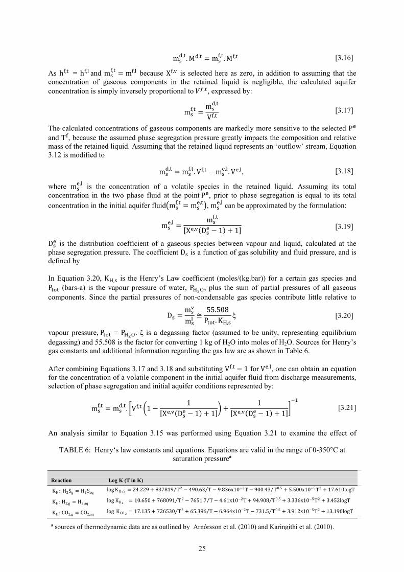
25
m , . M , = m , . M , [3.16]
As h , = h , and m , = m , because X , is selected here as zero, in addition to assuming that the concentration of gaseous components in the retained liquid is negligible, the calculated aquifer concentration is simply inversely proportional to , , expressed by:
The calculated concentrations of gaseous components are markedly more sensitive to the selected P and T , because the assumed phase segregation pressure greatly impacts the composition and relative mass of the retained liquid. Assuming that the retained liquid represents an ‘outflow’ stream, Equation 3.12 is modified to
where m , is the concentration of a volatile species in the retained liquid. Assuming its total concentration in the two phase fluid at the point P , prior to phase segregation is equal to its total concentration in the initial aquifer fluid m , = m , , m , can be approximated by the formulation:
D is the distribution coefficient of a gaseous species between vapour and liquid, calculated at the phase segregation pressure. The coefficient D is a function of gas solubility and fluid pressure, and is defined by In Equation 3.20, K , is the Henry’s Law coefficient (moles/(kg.bar)) for a certain gas species and P (bars-a) is the vapour pressure of water, P , plus the sum of partial pressures of all gaseous components. Since the partial pressures of non-condensable gas species contribute little relative to
vapour pressure, P = P . ξ is a degassing factor (assumed to be unity, representing equilibrium degassing) and 55.508 is the factor for converting 1 kg of H2O into moles of H2O. Sources for Henry’s gas constants and additional information regarding the gas law are as shown in Table 6. After combining Equations 3.17 and 3.18 and substituting V , − 1 for V , , one can obtain an equation for the concentration of a volatile component in the initial aquifer fluid from discharge measurements, selection of phase segregation and initial aquifer conditions represented by:
An analysis similar to Equation 3.15 was performed using Equation 3.21 to examine the effect of
m , = m ,V , [3.17]
m , = m , . V , − m , . V , , [3.18]
m , = m ,[X , (D − 1) + 1] [3.19]
D = mm ≅ 55.508P . K , ξ [3.20]
m , = m , . V , 1 − 1[X , (D − 1) + 1] + 1[X , (D − 1) + 1] [3.21]
TABLE 6: Henry‘s law constants and equations. Equations are valid in the range of 0-350°C at saturation pressureª
Reaction Log K (T in K) KH : H2Sg = H2Saq log KH2S = 24.229 + 837819 T2⁄ − 490.63 T⁄ − 9.836x10⁻²T − 900.43 T0.5⁄ + 5.500x10⁻⁵T2 + 17.610logT KH : H2,g = H2,aq log KH2 = 10.650 + 768091 T2⁄ − 7651.7 T⁄ − 4.61x10⁻²T + 94.908 T0.5⁄ + 3.336x10⁻⁵T2 + 3.452logT KH : CO2,g = CO2,aq log KCO 2 = 17.135 + 726530 T2⁄ + 65.396 T⁄ − 6.964x10⁻²T − 731.5 T0.5⁄ + 3.912x10⁻⁵T2 + 13.190logT
ª sources of thermodynamic data are as outlined by Arnórsson et al. (2010) and Karingithi et al. (2010).

26
assumed phase segregation pressure on calculated initial aquifer fluid gas (H2S, H2 and CO2) concentration (Figure 21). From this figure, a conclusion that the calculated concentration of a gaseous component is quite sensitive to the assumed phase segregation pressure but not so for the selected is made. Equations 3.19 and 3.21 assume that the volatile components are found in the liquid phase as a single species, whose solubility is described by the Henry’s law constant. However, CO2 and H2S can exist as dissociated weak acids; thus, the magnitude of pH change between the initial aquifer fluid and the phase segregation pressure affects the distribution of these components. Modelled initial aquifer fluid compositions In practice WATCH 2.1 (Arnórsson et al., 1982 and Bjarnason, 1994) was used to infer the initial aquifer fluids. WATCH 2.1 is suited to handle geochemical data from wet-steam wells. The program reads the chemical analyses of water and gas samples collected at the wellhead then computes for the chemical composition at the selected reference temperature including pH, aqueous speciation, partial pressure of gases, redox potentials and activity products of mineral dissolution reactions. No mineral precipitation or dissolution is assumed as the fluid is modelled from the aquifer to the surface. To model liquid enthalpy wells the analytical data were input into WATCH 2.1, excluding the measured discharge enthalpy then iterated the selected reference temperature until the total silica concentration in the liquid aquifer was consistent with T . The 1st step in modelling the excess enthalpy wells was done by inputting both analytical data and measured discharge enthalpy then choosing a reference temperature, in this case, T (equivalent to the selected segregation pressure, P ). The output of WATCH 2.1 by this 1st step is picked up to become the input file of the 2nd step. When executing the 2nd step, no enthalpy will be input as it is calculated from the reference temperature, then iterating the input until the total silica concentration in the liquid aquifer is consistent with T . The modelled liquid enthalpy aquifers feeding the Námafjall wells as described by the above procedures are summarized in Table 7. For comparison with Figures 20 and 21, the aquifer fluid concentrations of silica and the main gases (CO2, H2S and H2) at different assumed phase segregation pressures are calculated and shown for a few representative well discharges in Figures 22 and 23, respectively. Figure 22 shows the modelled initial aquifer SiO2 concentration, in mg/kg, of the excess enthalpy wells, considering various selected phase segregation pressures. The computed gas concentrations in the deep liquid in log units as a function of phase segregation pressures are illustrated in Figure 23. From Figure 23 it is evident that the calculated concentration of a gaseous component in the initial aquifer fluid is quite sensitive to the assumed phase segregation pressure, even at relatively low excess discharge enthalpies. The selected phase segregation pressure described in Section 3.3.3 are considered to be reasonable in light of consideration of the liquid saturation after boiling from T (given by pressure P ) to P . It should be noted that the selected phase segregation pressure corresponds to residual liquid saturation of 0.2 which is an extreme limit for liquid immobility (see Section 3.3.3). In this case the pressures lower than the indicated P would be unlikely to select and the calculated values not representative in light of this discussion. Liquid saturation at the phase segregation pressure is fairly consistent; approximately the residual liquid saturation as shown by Corey curves (Figure 17). A slight extent of phase segregation may be expected to take place before the residual liquid saturation has been reached during depressurization boiling. In that case, the selected phase segregation pressure may overestimate the initial aquifer fluid gas concentrations.
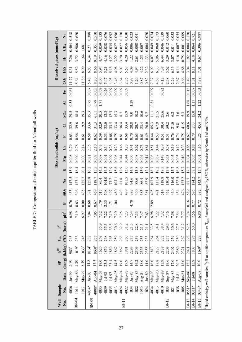
27
BS
iO2
Na
KM
gC
aF
Cl
SO4
Al
FeC
O2
H2S
H2
CH
4N
2
4036
Jun-
993.
7098
3a24
56.
980.
7643
514
7.5
15.9
0.00
83.
790.
6332
.929
.50.
550.
064
11.7
78.
317.
260.
404
0.51
8
1014
May
-86
5.20
1019
a23
37.
190.
6339
612
7.1
18.4
0.00
02.
780.
5639
.618
.45.
645.
523.
720.
986
0.62
0
1012
Mar
-79
8.10
1033
a24
56.
970.
0043
512
5.7
20.1
0.00
02.
140.
6119
.919
.311
.36
8.99
11.6
41.
681
4034
*Ju
n-07
11.8
1014
a23
27.
040.
6839
112
5.8
16.2
0.08
12.
350.
5833
.635
.30.
750.
007
5.48
6.83
6.34
0.27
10.
388
4008
*A
pr-0
413
.510
60a
255
7.05
0.67
469
118.
715
.50.
009
2.10
0.62
31.3
61.1
0.79
0.00
58.
308.
669.
190.
351
0.51
040
33M
ay-0
319
.016
2026
935
.97.
121.
7951
786
.414
.50.
008
0.43
0.59
32.9
20.5
1.71
0.00
98.
005.
944.
770.
059
0.13
840
59Ju
l-98
23.5
1850
268
35.3
7.22
2.35
508
104.
014
.30.
001
0.34
0.53
33.0
12.3
0.02
65.
475.
214.
160.
038
0.07
640
35Ju
l-97
23.1
1850
265
33.5
7.19
1.71
497
77.2
12.9
0.00
90.
230.
6833
.512
.30.
009
4.95
5.15
4.27
0.03
50.
092
4013
May
-95
14.5
1867
259
30.6
7.29
1.04
480
103.
115
.80.
008
0.23
0.75
33.4
15.3
0.00
93.
464.
983.
220.
027
0.09
640
24M
ay-9
419
.018
6726
332
.97.
2549
381
.812
.90.
044
0.46
0.81
36.4
8.7
0.00
93.
645.
073.
700.
027
0.17
040
22M
ay-9
319
.919
8126
031
.27.
2347
910
1.5
13.6
0.04
40.
230.
6833
.415
.90.
009
2.75
5.57
4.20
0.05
60.
030
1034
Jun-
8514
.722
9323
521
.57.
544.
7038
794
.614
.90.
000
0.41
0.70
20.8
9.0
1.29
0.97
4.09
1.22
0.00
60.
023
1022
May
-83
16.2
2309
239
22.8
7.33
400
88.6
13.8
0.00
80.
620.
6320
.710
.21.
204.
942.
610.
008
0.04
110
50A
ug-8
118
.023
5523
521
.57.
4738
586
.413
.90.
004
0.73
0.61
23.4
10.6
0.87
4.22
1.25
0.00
710
24Ju
n-80
11.0
2355
233
21.1
7.63
381
82.9
12.1
0.01
40.
810.
4926
.09.
20.
822.
321.
330.
004
0.02
040
34M
ay-0
316
.018
1326
433
.56.
982.
8949
510
7.9
18.7
0.00
80.
510.
4485
.311
.10.
510.
009
7.37
6.92
6.07
0.04
90.
074
4013
May
-90
17.8
2127
264
34.1
7.22
491
131.
418
.20.
037
0.44
0.53
67.9
21.5
4.68
6.33
5.96
0.06
80.
173
4010
May
-89
15.9
2138
272
38.4
7.32
514
118.
817
.50.
149
0.39
0.51
30.4
25.6
0.08
34.
137.
386.
440.
046
0.13
910
33S
ep-8
719
.622
0325
729
.57.
4646
213
0.4
17.9
0.05
30.
580.
5159
.22.
62.
585.
623.
290.
012
0.06
010
21M
ay-8
317
.024
0225
930
.67.
5846
011
6.0
15.7
0.00
50.
190.
7621
.06.
22.
296.
133.
070.
011
0.05
310
38Ju
l-81
20.2
2380
250
27.5
7.54
434
122.
516
.80.
003
0.12
0.74
9.8
3.6
2.67
6.14
4.16
0.00
70.
055
1005
Mar
-81
18.0
2321
262
31.2
7.77
476
123.
215
.70.
016
0.33
0.75
41.5
5.3
0.66
4.68
0.75
0.00
10.
009
BJ-
1305
51*
Sep
-06
15.2
2021
293
52.5
7.74
0.16
589
87.7
17.2
0.00
40.
850.
6260
.619
.91.
680.
015
1.49
3.04
1.92
0.00
40.
170
BJ-
1403
11*
Jul-
0815
.918
0729
550
.07.
560.
7759
518
4.2
38.1
0.00
30.
880.
7920
015
.01.
170.
007
1.81
8.11
4.18
0.06
40.
721
BJ-
1503
43*
Aug
-08
10.0
1169
a22
96.
800.
7238
214
3.7
15.7
0.00
11.
161.
2545
.424
.21.
220.
003
7.38
7.01
9.67
0.39
60.
987
BJ-
12
pHb
hd,t
(kJ/
kg)
a liq
uid
enth
alpy
wel
l sam
ples
, b pH a
t aqu
ifer t
empe
ratu
re T
qtz,
*sa
mpl
ed a
nd a
naly
sed
by IS
OR
, oth
erw
ise b
y K
emia
Ltd
and
NEA
.
BN
-04
BN
-09
BJ-
11
SP
(b
ar-g
)W
ell
No.
Sam
ple
No.
Dat
eT
qtz
(°C
)Pe
(bar
-a)
Dis
solv
ed s
olid
s (m
g/kg
)D
isso
lved
gas
es (
mm
ol/k
g)
TA
BL
E 7
: C
ompo
siti
on o
f in
itia
l aqu
ifer
flu
id f
or N
ámaf
jall
wel
ls
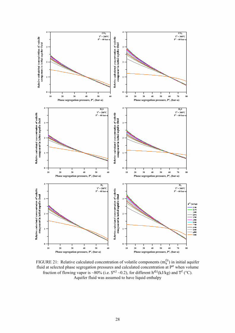
28
FIGURE 21: Relative calculated concentration of volatile components (m , ) in initial aquifer fluid at selected phase segregation pressures and calculated concentration at P when volume
fraction of flowing vapor is ~80% (i.e. S , ~0.2), for different h , (kJ/kg) and T (°C). Aquifer fluid was assumed to have liquid enthalpy
10 20 30 40 50 60
Phase segregation pressure, Pe, (bar-a)
0
1
2
3
4 CO2
Tf = 280oCPe ~ 40 bar-a
10 20 30 40 50 60 70 80
Phase segregation pressure, Pe, (bar-a)
0
1
2
3
4 CO2
Tf = 300oCPe ~ 60 bar-a
10 20 30 40 50 60
Phase segregation pressure, Pe, (bar-a)
0
1
2
3
4 H2S
Tf = 280oCPe ~ 40 bar-a
10 20 30 40 50 60 70 80
Phase segregation pressure, Pe, (bar-a)
0
1
2
3
4 H2S
Tf = 300oCPe ~ 60 bar-a
10 20 30 40 50 60
Phase segregation pressure, Pe, (bar-a)
0
1
2
3
4 H2
Tf = 280oCPe ~ 40 bar-a
10 20 30 40 50 60 70 80
Phase segregation pressure, Pe, (bar-a)
0
1
2
3
4 H2
Tf = 300oCPe ~ 60 bar-a
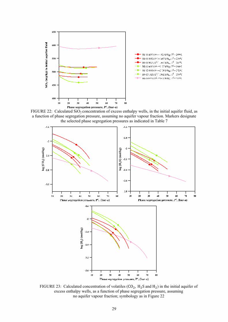
29
FIGURE 23: Calculated concentration of volatiles (CO , H S and H ) in the initial aquifer of
excess enthalpy wells, as a function of phase segregation pressure, assuming no aquifer vapour fraction; symbology as in Figure 22
log
[CO
2](m
ol/k
g)
log
[H2S
](m
ol/k
g)
log
[H2]
(mol
/kg)
FIGURE 22: Calculated SiO2 concentration of excess enthalpy wells, in the initial aquifer fluid, as a function of phase segregation pressure, assuming no aquifer vapour fraction. Markers designate
the selected phase segregation pressures as indicated in Table 7
10 20 30 40 50 60 70 80
Phase segregation pressure, Pe, (bar-a)
400
450
500
550
600
650
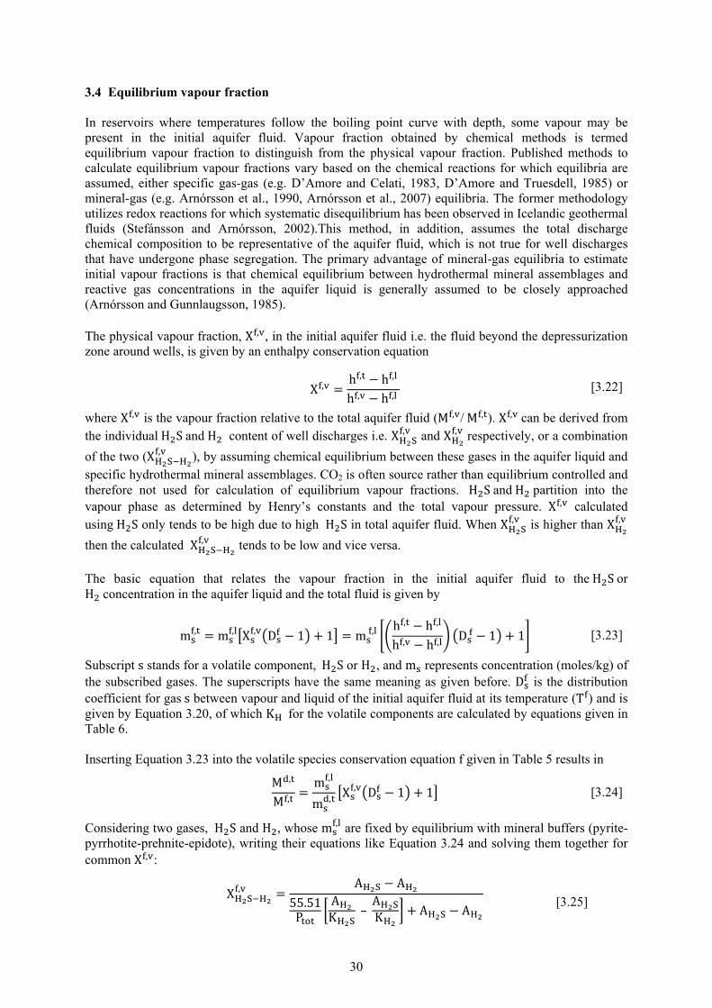
30
3.4 Equilibrium vapour fraction In reservoirs where temperatures follow the boiling point curve with depth, some vapour may be present in the initial aquifer fluid. Vapour fraction obtained by chemical methods is termed equilibrium vapour fraction to distinguish from the physical vapour fraction. Published methods to calculate equilibrium vapour fractions vary based on the chemical reactions for which equilibria are assumed, either specific gas-gas (e.g. D’Amore and Celati, 1983, D’Amore and Truesdell, 1985) or mineral-gas (e.g. Arnórsson et al., 1990, Arnórsson et al., 2007) equilibria. The former methodology utilizes redox reactions for which systematic disequilibrium has been observed in Icelandic geothermal fluids (Stefánsson and Arnórsson, 2002).This method, in addition, assumes the total discharge chemical composition to be representative of the aquifer fluid, which is not true for well discharges that have undergone phase segregation. The primary advantage of mineral-gas equilibria to estimate initial vapour fractions is that chemical equilibrium between hydrothermal mineral assemblages and reactive gas concentrations in the aquifer liquid is generally assumed to be closely approached (Arnórsson and Gunnlaugsson, 1985). The physical vapour fraction, X , , in the initial aquifer fluid i.e. the fluid beyond the depressurization zone around wells, is given by an enthalpy conservation equation
where X , is the vapour fraction relative to the total aquifer fluid (M , / M , ). X , can be derived from the individual H S and H content of well discharges i.e. X , and X , respectively, or a combination
of the two (X , ), by assuming chemical equilibrium between these gases in the aquifer liquid and specific hydrothermal mineral assemblages. CO2 is often source rather than equilibrium controlled and therefore not used for calculation of equilibrium vapour fractions. H S and H partition into the vapour phase as determined by Henry’s constants and the total vapour pressure. X , calculated using H S only tends to be high due to high H S in total aquifer fluid. When X , is higher than X ,
then the calculated X , tends to be low and vice versa. The basic equation that relates the vapour fraction in the initial aquifer fluid to the H S or H concentration in the aquifer liquid and the total fluid is given by
Subscript s stands for a volatile component, H S or H , and m represents concentration (moles/kg) of the subscribed gases. The superscripts have the same meaning as given before. D is the distribution coefficient for gas s between vapour and liquid of the initial aquifer fluid at its temperature (T ) and is given by Equation 3.20, of which K for the volatile components are calculated by equations given in Table 6. Inserting Equation 3.23 into the volatile species conservation equation f given in Table 5 results in
M ,M , = m ,m , X , D − 1 + 1 [3.24]
Considering two gases, H S and H , whose m , are fixed by equilibrium with mineral buffers (pyrite-pyrrhotite-prehnite-epidote), writing their equations like Equation 3.24 and solving them together for common X , :
X , = h , − h ,h , − h , [3.22]
m , = m , X , D − 1 + 1 = m , h , − h ,h , − h , D − 1 + 1 [3.23]
X , = A − A55.51P AK – AK + A − A
[3.25]

31
where A = m , / m , and A = m , /m , ; m , and m , are measured; m , and m , are taken to be known
functions of temperature, T (oC), as are K and K (Henry‘s law coefficients for H S and H respectively). After deriving an equilibrium vapour fraction, X , (Table 8 and Figure 24) the total aquifer fluid enthalpy (h , ) is no longer equal to h , , but can be solved using the relationship given by Equation 3.22. Albeit liquid enthalpy exhibited by some of the wells, X , values for these wells were also calculated, and a phase segregation pressure chosen in the same way as calculated for the ‘excess’ enthalpy wells. From Figure 24a, it is evident that the calculated equilibrium vapour fractions are dependent on the initial aquifer fluid temperature and in turn to the assumed phase segregation pressure. Taking the wells with long production period, the equilibrium vapour fraction seems to be increasing over time (Table 8), but the increase is relatively small e.g. for well BJ-11 a wt. % X , increase from 0.05 to 1.21 has been observed in the time period of about 20 years. An overestimation of the initial aquifer temperature by ±10°C would result in a relatively small overestimation or
FIGURE 24: Calculated equilibrium vapour fractions (X , ) for Námafjall wells as
a function of: (a) aquifer temperature, and (b) time; symbology as in Figure 14
wt.
%X
f,v
a.
wt.
%X
f,v
b.
TABLE 8: Calculated equilibrium vapour fractions for Námafjall wells
Well No.
Sample No
hd,t
(kJ/kg)
Tqtz
(oC)
wt. %
Xf,vH2
wt. %
Xf,vH2S_H2
4036 983a 245 1.85 0.12
1014 1019a 233 0.90 0.03
1012 1033a 245 3.05 0.304034* 1014a 232 1.61 0.08
4008* 1060a 255 2.37 0.314033 1620 269 1.07 1.124059 1850 268 0.90 1.214035 1850 265 0.95 1.084013 1867 259 0.68 0.604024 1867 263 0.79 0.854022 1981 260 0.95 0.761034 2293 235 0.22 0.061022 2309 239 0.59 0.191050 2355 235 0.23 0.051024 2355 233 0.25 0.254034 1813 264 1.46 0.994013 2127 264 1.43 1.614010 2138 272 1.53 2.081033 2203 257 0.71 0.591021 2402 259 0.64 0.611038 2380 250 0.98 0.801005 2321 262 -0.03 0.00
BJ-13 0551* 2021 293 -0.02 3.90BJ-14 0311* 1807 295 0.64 1.89
BJ-15 0343* 1169a 229 2.51 0.161.05 0.79
BN-04
BN-09
BJ-11
BJ-12
Average:a liquid enthalpy well samples, *sampled and analysed by ÍSOR, otherwise by Kemia Ltd and NEA.
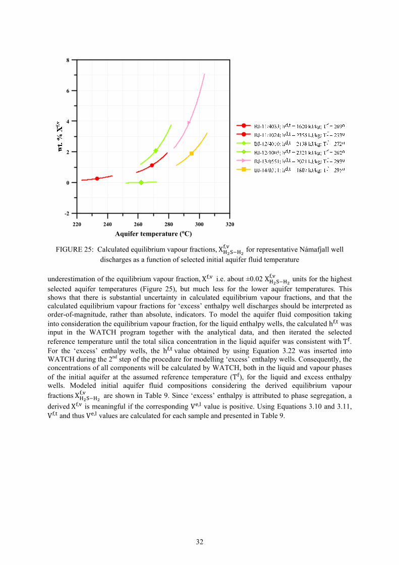
32
underestimation of the equilibrium vapour fraction, X , i.e. about ±0.02 X , units for the highest selected aquifer temperatures (Figure 25), but much less for the lower aquifer temperatures. This shows that there is substantial uncertainty in calculated equilibrium vapour fractions, and that the calculated equilibrium vapour fractions for ‘excess’ enthalpy well discharges should be interpreted as order-of-magnitude, rather than absolute, indicators. To model the aquifer fluid composition taking into consideration the equilibrium vapour fraction, for the liquid enthalpy wells, the calculated h , was input in the WATCH program together with the analytical data, and then iterated the selected reference temperature until the total silica concentration in the liquid aquifer was consistent with T . For the ‘excess’ enthalpy wells, the h , value obtained by using Equation 3.22 was inserted into WATCH during the 2nd step of the procedure for modelling ‘excess’ enthalpy wells. Consequently, the concentrations of all components will be calculated by WATCH, both in the liquid and vapour phases of the initial aquifer at the assumed reference temperature (T ), for the liquid and excess enthalpy wells. Modeled initial aquifer fluid compositions considering the derived equilibrium vapour fractions X , are shown in Table 9. Since ‘excess’ enthalpy is attributed to phase segregation, a
derived X , is meaningful if the corresponding V , value is positive. Using Equations 3.10 and 3.11, V , and thus V , values are calculated for each sample and presented in Table 9.
FIGURE 25: Calculated equilibrium vapour fractions, X , for representative Námafjall well discharges as a function of selected initial aquifer fluid temperature
220 240 260 280 300 320
Aquifer temperature (oC)
-2
0
2
4
6
8
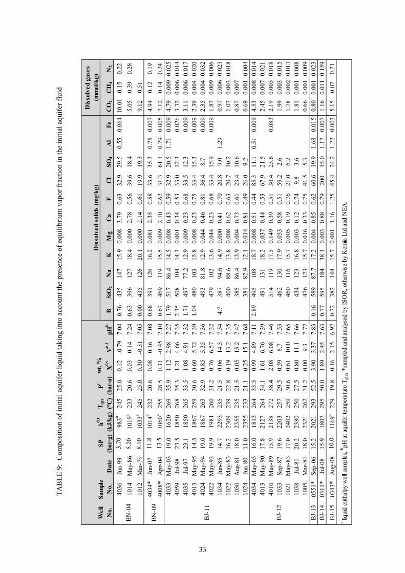
33
BS
iO2
Na
KM
gC
aF
Cl
SO
4A
lF
eC
O2
CH
4N
2
4036
Jun-
993.
7098
3a24
525
.00.
12-0
.79
7.04
0.76
435
147
15.9
0.00
83.
790.
6332
.929
.50.
550.
064
10.0
10.
150.
22
1014
May
-86
5.20
1019
a23
320
.60.
030.
147.
240.
6339
612
718
.40.
000
2.78
0.56
39.6
18.4
5.05
0.39
0.28
1012
Mar
-79
8.10
1033
a24
525
.00.
30-0
.31
7.05
0.00
435
126
20.1
0.00
02.
140.
6119
.919
.39.
120.
51
4034
*Ju
n-07
11.8
1014
a23
220
.60.
080.
167.
080.
6839
112
616
.20.
081
2.35
0.58
33.6
35.3
0.75
0.00
74.
940.
120.
19
4008
*A
pr-0
413
.510
60a
255
28.5
0.31
-0.4
57.
100.
6746
911
915
.50.
009
2.10
0.62
31.3
61.1
0.79
0.00
57.
120.
140.
2440
33M
ay-0
319
.016
2026
935
.91.
122.
987.
271.
7951
786
.414
.50.
008
0.43
0.59
32.9
20.5
1.71
0.00
94.
790.
009
0.02
540
59Ju
l-98
23.5
1850
268
35.3
1.21
4.66
7.35
2.35
508
104
14.3
0.00
10.
340.
5333
.012
.30.
026
3.32
0.00
60.
014
4035
Jul-
9723
.118
5026
533
.51.
084.
917.
321.
7149
777
.212
.90.
009
0.23
0.68
33.5
12.3
0.00
93.
110.
006
0.01
740
13M
ay-9
514
.518
6725
930
.60.
605.
727.
391.
0448
010
315
.80.
008
0.23
0.75
33.4
15.3
0.00
92.
390.
004
0.02
040
24M
ay-9
419
.018
6726
332
.90.
855.
357.
3649
381
.812
.90.
044
0.46
0.81
36.4
8.7
0.00
92.
350.
004
0.03
240
22M
ay-9
319
.919
8126
031
.20.
766.
577.
3247
910
213
.60.
044
0.23
0.68
33.4
15.9
0.00
91.
870.
009
0.00
610
34Ju
n-85
14.7
2293
235
21.5
0.06
14.5
7.54
4.7
387
94.6
14.9
0.00
00.
410.
7020
.89.
01.
290.
970.
006
0.02
310
22M
ay-8
316
.223
0923
922
.80.
1913
.27.
3540
088
.613
.80.
008
0.62
0.63
20.7
10.2
1.07
0.00
30.
018
1050
Aug
-81
18.0
2355
235
21.5
0.05
15.2
7.47
385
86.4
13.9
0.00
40.
730.
6123
.410
.60.
870.
007
1024
Jun-
8011
.023
5523
321
.10.
2515
.17.
6838
182
.912
.10.
014
0.81
0.49
26.0
9.2
0.69
0.00
10.
004
4034
May
-03
16.0
1813
264
33.5
0.99
4.89
7.11
2.89
495
108
18.7
0.00
80.
510.
4485
.311
.10.
510.
009
4.53
0.00
80.
014
4013
May
-90
17.8
2127
264
34.1
1.61
6.76
7.39
491
131
18.2
0.03
70.
440.
5367
.921
.52.
450.
007
0.02
140
10M
ay-8
915
.921
3827
238
.42.
086.
087.
4651
411
917
.50.
149
0.39
0.51
30.4
25.6
0.08
32.
190.
005
0.01
810
33S
ep-8
719
.622
0325
729
.50.
598.
77.
5346
213
017
.90.
053
0.58
0.51
59.2
2.6
1.99
0.00
30.
015
1021
May
-83
17.0
2402
259
30.6
0.61
10.0
7.65
460
116
15.7
0.00
50.
190.
7621
.06.
21.
780.
002
0.01
310
38Ju
l-81
20.2
2380
250
27.5
0.80
11.1
7.66
434
123
16.8
0.00
30.
120.
749.
83.
61.
810.
001
0.00
810
05M
ar-8
118
.023
2126
231
.20.
009.
37.
7747
612
315
.70.
016
0.33
0.75
41.5
5.3
0.66
0.00
10.
009
BJ-
1305
51*
Sep
-06
15.2
2021
293
52.5
3.90
3.37
7.83
0.16
589
87.7
17.2
0.00
40.
850.
6260
.619
.91.
680.
015
0.80
0.00
10.
023
BJ-
1403
11*
Jul-
0815
.918
0729
550
.01.
892.
457.
630.
7759
518
438
.10.
003
0.88
0.79
200
15.0
1.17
0.00
71.
160.
011
0.15
9
BJ-
1503
43*
Aug
-08
10.0
1169
a22
919
.80.
162.
156.
920.
7238
214
415
.70.
001
1.16
1.25
45.4
24.2
1.22
0.00
35.
150.
070.
21
Dis
solv
ed g
ases
(m
mol
/kg)
a liq
uid
enth
alpy
wel
l sam
ples
, b pH a
t aqu
ifer
tem
pera
ture
Tqt
z, *
sam
pled
and
ana
lyse
d by
IS
OR
, oth
erw
ise
by K
emia
Ltd
and
NE
A.
BN
-04
BN
-09
BJ-
11
BJ-
12
Dis
solv
ed s
olid
s (m
g/k
g)W
ell
No.
Sam
ple
No.
Dat
eT
qtz
(°C
)P
e
(bar
-a)
wt.
%
Xf,
vhd,
t
(kJ/
kg)
Ve,
lS
P
(b
ar-g
)pH
b
TA
BL
E 9
: C
ompo
siti
on o
f in
itia
l aqu
ifer
liqu
id ta
king
into
acc
ount
the
pres
ence
of
equi
libr
ium
vap
or f
ract
ion
in th
e in
itia
l aqu
ifer
flu
id
34
4. MINERAL-GAS-LIQUID EQUILIBRIA Appraisal of the chemical evolution of hydrothermal fluids and of the extent to which the fluids have approached equilibrium according to certain chemical reactions is based on the concept of local equilibrium within the larger open geothermal system, analytical data on the composition of well discharges, modelling of aquifer fluid compositions and thermodynamic data on gases, aqueous species and minerals. An emphasis on the underlying assumptions and simplifications before interpreting the equilibrium state of the aquifer fluid at Námafjall is that: the samples collected at the wellhead are taken to represent the deep aquifers feeding the well and no dissolution or precipitation reactions occur between the initial aquifer fluids and wellhead, and that the selection of T , is reasonable. In addition, aqueous speciation distribution of the aquifer fluid uses thermodynamic databases that carry uncertainties. Assuming the concept of local equilibrium within the larger open geothermal system allows the application of thermodynamic principles to assess how closely local equilibrium conditions are approached based on the geochemical data of the modelled aquifers. 4.1 Alteration mineralogy and thermodynamic data Alteration mineralogy in the high-temperature geothermal systems in Iceland has been summarized by Arnórsson (1995). All Icelandic geothermal fields show a zonation with depth reflecting the temperature stability range of the minerals within the system. Calcite is stable but disappears at temperatures above ~ 280°C and pyrite is stable over the whole range of temperature. Chalcedony is stable up to ~180°C but above that temperature quartz is the dominant silica polymorph. Prehnite appears above 200°C and epidote at slightly higher temperature (Hreggvidsdóttir, 1987; Lonker et al., 1993). Albite is common, especially at temperatures above 150°C, whereas K-feldspar (adularia) is scarce, due to the low K content of the host rocks. Hydrothermal sheet silicates are represented by smectite interstratified with chlorite above 200°C, and above 230-240°C discrete chlorite is formed. Garnet, represented by the grossular-andradite solid solution is widely present in high saline fluids (Lonker et al., 1993; Giroud, 2008). Magnetite is mostly present as a primary mineral but is generally unstable in high-temperature geothermal systems. Gudmundsson and Arnórsson (2005), Isabirye (1994) and Kristmannsdóttir (1978) have studied the alteration minerals in the Námafjall geothermal system and indicate the occurrence of albite, calcite, chlorite, epidote, K-feldspar (adularia), prehnite, pyrite, pyrrhotite, quartz and wairakite. Garnet has been reported as a mineral formed by contact metamorphism. Its presence is considered to be the consequence of extensive boiling of the aquifer water in response to intrusion of magma forming small intrusive bodies within the geothermal system. Námafjall waters are under-saturated with respect to anhydrite and Gudmundsson and Arnórsson (2005) conclude that the stability of anhydrite is considered to be linked with that of epidote. Frauke et al., 2008 studied CO fixation by calcite in the Icelandic high-temperature fields and concluded that vast amounts of CO and thus calcite is distributed in the upper 1km of the three fields considered. The thermodynamic database selected for this study plays an essential role for both the speciation calculations performed by WATCH 2.1 and to interpret the saturation state of the aquifer with respect to different mineral-fluid reactions that could potentially control the composition of aquifer fluids. The saturation state of the aquifer liquid is assessed for hydrothermal alteration minerals, and several potential mineral pair and assemblages evaluated for their potential to control selected activity ratios and gas species concentrations in the initial aquifer fluid. The thermodynamic data base used for speciation calculations is that depicted in Arnórsson et al. (1982) with slight modifications. The reactions considered and equations describing the temperature dependence of their equilibrium constants are shown in Tables 10 and 11, for the mineral pairs or assemblages and the individual alteration minerals, respectively. Equilibrium constants for the reactions given in Tables 10 and 11 are based on thermodynamic data (∆G°, S°, V°, C° ) of the minerals from Holland and Powell (1998) except for pyrite, pyrrhotite and calcite. Data on the sulfide minerals were taken from Robie and Hemingway (1995) and calcite

35
M
iner
al
Sym
bol
D
isso
luti
on r
eact
ion
L
og K
(T
in K
)
1.
And
radi
te
and
Ca 3Fe 2Si 3O 12
+4H+ +8H 2O(l)=3C
a+2 +2Fe(OH) 4− +3H 4S
iO 40 +940.2
25−15419.3
T⁄ +0.58092
T −2.971X10⁻⁴ T2 −421.
727logT
2.
Anh
ydri
te*
anh
4=+2 + 4−2
+78.414−32
47.2T⁄−9.03
X10−7 T2 −28.723logT
3.
Cal
cite
ca
l CaCO 3
+2H+ =Ca+2 +H 2O (l)+CO
2 (aq)
−68.271+43
85.24T⁄ −7
.525x10−3 T+25
.856logT
4.
Clin
ozoi
site
cz
o Ca 2Al 3
Si 3O 12(OH) +
12H 2O(l)=2C
a+2 +3Al(OH) 4− +3H 4S
iO 40 +OH− +36.05
2−6854.78
T⁄ +0.13236
T −1.3749X10⁻⁴ T2 +33.5
08logT
5.
Epi
dote
ep
i Al 2FeS
i 3O 12( OH) +1
2H 2O (l)=2Ca
+2 +Fe(OH) 4− +2Al(
OH) 4− +3H 4SiO 40 +OH−
+893.547−2
7077.4T⁄ +0
.154124T−3
.022x10−4 T2 −398.
38logT
6.
Gro
ssul
ar
gro
Ca 3Al 2Si 3O 12
+4H+ +8H 2Ol=3Ca
+2 +2Al(OH) 4− +3H 4S
iO 40 −571.6
62+17623.7
T⁄ −0.14343
T−203.808lo
gT 7.
M
agne
tite
mag
Fe 3O 4+
4H 2O (l)=Fe+2 +2Fe(
OH) 4− +949.9
51−24258.2
T⁄ +0.51474
T−2.402x10⁻⁴ T2 −417.
136logT
8.
Preh
nite
pr
e Ca 2Al 2
Si 3O 10(OH) 2+
10H 2O(l)=2C
a+2 +2Al(OH) 4− +3H 4S
iO 40 +OH− +833.9
5−25642.8
T⁄ +0.5035T
−2.941x10⁻⁴ T2 −369.
297logT
9.
Pyri
te
pyr
FeS 2+2H+ +H 2 (a
q)=Fe+2 +2H 2S
0 (l) −1.397
−461.3T⁄ −
9.128x10⁻⁴ T+1.6
26logT
10.
Pyrr
hoti
te
pyrr
FeS+2
H+ =Fe+2 +H 2S (aq)
−3.043+1579
.06T⁄ −1.987x
10−3 T+0.12logT
11.
Qua
rtz
qtz
SiO 2+2H 2O l
=H 4SiO 40
−34.188+19
7.47T⁄−5.85
1x10⁻⁶ T2 +12.245logT
12.
Wol
last
onit
e w
ol
CaSiO 3+H 2O (
l)+2H+ =Ca+2 +H 4Si
O 40 −127.0
96+8151.38
T⁄ −2.981x1
0−2 T+49.282log
T ª s
ourc
es o
f th
erm
odyn
amic
dat
a ar
e as
out
line
d by
Arn
órss
on a
nd S
tefa
nsso
n (1
999)
and
Kar
ingi
thi e
t al.
(201
0), *
fro
m G
udm
unds
son
and
Arn
órss
on (
2005
).
TA
BL
E 1
0. T
empe
ratu
re e
quat
ions
for
equ
ilib
rium
con
stan
ts f
or in
divi
dual
min
eral
dis
solu
tion
rea
ctio
ns. V
alid
in th
e ra
nge
0-35
0°C
at P
sat.
Uni
t act
ivit
y w
as s
elec
ted
for
all m
iner
als
and
liqu
id w
ater
a
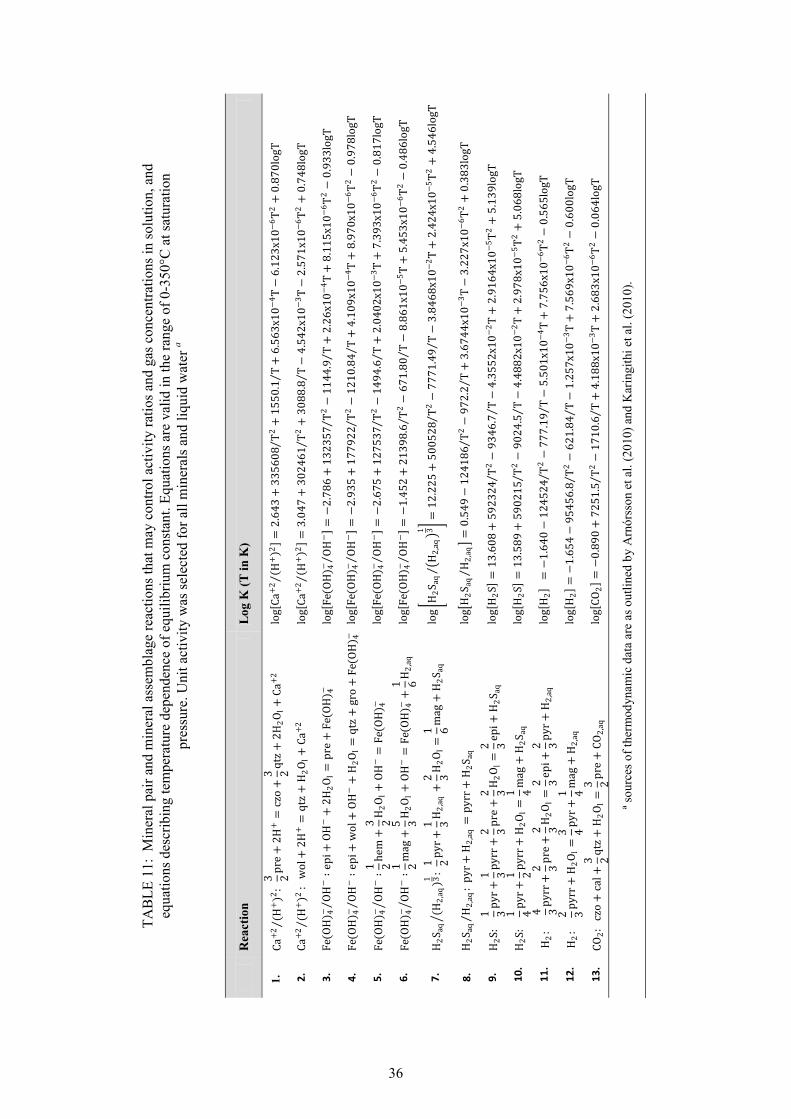
36
Rea
ctio
n
Log
K (
T in
K)
1.
Ca+2 (H+ )2 :
⁄3 2pre+2
H+ =czo+3 2qtz+2
H 2O l+Ca+2
log[ Ca+2 ( H+ )2 ⁄] =2.6
43+335608
T2 ⁄ +1550.1
T⁄ +6.563x1
0−4 T−6.123x10⁻⁶ T2 +0.87
0logT 2.
Ca+2 (H+ )2 ⁄: wol+
2H+ =qtz+H 2O l+
Ca+2 log[ Ca+2 ( H+ )2 ⁄
] =3.047+3
02461T2 ⁄ +
3088.8T⁄ −4
.542x10−3 T−2.5
71x10−6 T2 +0.748logT
3.
Fe(OH)
4− OH− ∶epi+OH− +2H 2O
l=pre+Fe(O
H) 4−⁄
log[ Fe(
OH) 4− OH− ⁄]=−2.7
86+132357
T2 ⁄ −1144.9
T⁄ +2.26x10
−4 T+8.115x10⁻⁶ T2 −0.93
3logT 4.
Fe(OH)4− OH− ∶epi+
wol+OH− +H 2O l
=qtz+gro+F
e(OH) 4−⁄
log[ Fe(
OH) 4− OH− ⁄]=−2.9
35+177922
T2 ⁄ −1210.8
4T⁄ +4.109x
10−4 T+8.970x10⁻⁶ T2 −0.97
8logT 5.
Fe(OH)4− OH− ∶1 2hem+
3 2H 2O l + OH− =Fe(O
H) 4− log[ Fe(
OH) 4− OH− ⁄]=−2.6
75+127537
T2 ⁄ −1494.6
T⁄ +2.0402x
10−3 T+7.393x10⁻⁶ T2 −0.81
7logT 6.
Fe(OH)4− OH− ∶1 2mag+
5 3H 2O l+OH− =Fe(O
H) 4− +1 6H 2,aq log[ Fe(
OH) 4− OH− ⁄]=−1.4
52+21398.6
T2 ⁄ −671.80
T⁄ −8.861x1
0−5 T+5.453x10⁻⁶ T2 −0.48
6logT 7.
H 2S aq(H 2,aq)
1 3 : 1 2pyr+1 3H 2,aq+2 3H 2O l=
1 6mag+H 2S aq
logH 2S aqH
2,aq1 3⁄
=12.225+5
00528T2 ⁄ −
7771.49T⁄ −
3.8468x10⁻² T+2.4
24x10−5 T2 +4.546logT
8.
H 2S aq
H 2,aq: pyr+H
2,aq=pyrr+H
2S aq⁄
logH 2
S aqH 2,aq⁄
=0.549−12
4186T2 ⁄ −
972.2T⁄ +3
.6744x10−3 T−3.2
27x10−6 T2 +0.383logT
9.
H 2S:
1 3pyr+1 3pyrr+2 3pre+2 3H 2O l=
2 3epi+H2S aq
log[ H 2S] =13.
608+59232
4T2 ⁄ −9346.7
T⁄ −4.3552x
10−2 T+2.9164x10
−5 T2 +5.139logT
10.
H 2S:
1 4pyr+1 2pyrr+H 2O l=
1 4mag+H 2S aq
log[ H 2S] =13.
589+59021
5T2 ⁄ −9024.5
T⁄ −4.4882x
10−2 T+2.978x10⁻⁵ T2 +5.06
8logT 11
.
H 2: 4 3pyrr+
2 3pre+2 3H 2O l=2 3epi+2 3pyr+H
2,aq log[ H 2]
=−1.640−
124524T2 ⁄ −
777.19T⁄ −5
.501x10−4 T+7.7
56x10−6 T2 −0.565logT
12.
H 2:
2 3pyrr+H 2O l=
3 4pyr+1 4mag+H 2,aq
log[ H 2]=−1.6
54−95456.8
T2 ⁄ −621.84
T⁄ −1.257x1
0−3 T+7.569x10⁻⁶ T2 −0.60
0logT 13
.
CO 2: czo+ca
l+3 2qtz+H2O l=3 2pre+C
O 2,aq log[ CO
2] =−0.890+
7251.5T2 ⁄ −
1710.6T⁄ +4
.188x10−3 T+2.6
83x10−6 T2 −0.064logT
ª sou
rces
of
ther
mod
ynam
ic d
ata
are
as o
utli
ned
by A
rnór
sson
et a
l. (2
010)
and
Kar
ingi
thi e
t al.
(201
0).
TA
BL
E 1
1: M
iner
al p
air
and
min
eral
ass
embl
age
reac
tion
s th
at m
ay c
ontr
ol a
ctiv
ity
rati
os a
nd g
as c
once
ntra
tion
s in
sol
utio
n, a
nd
equa
tion
s de
scri
bing
tem
pera
ture
dep
ende
nce
of e
quil
ibri
um c
onst
ant.
Equ
atio
ns a
re v
alid
in th
e ra
nge
of 0
-350
°C a
t sat
urat
ion
pres
sure
. Uni
t act
ivit
y w
as s
elec
ted
for
all m
iner
als
and
liqu
id w
ater
a
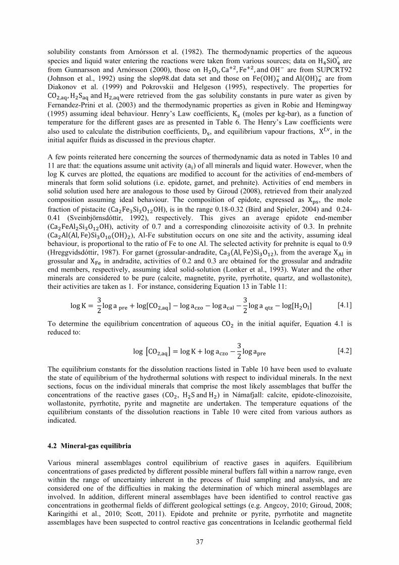
37
solubility constants from Arnórsson et al. (1982). The thermodynamic properties of the aqueous species and liquid water entering the reactions were taken from various sources; data on H SiO° are from Gunnarsson and Arnórsson (2000), those on H O , Ca , Fe , and OH are from SUPCRT92 (Johnson et al., 1992) using the slop98.dat data set and those on Fe(OH) and Al(OH) are from Diakonov et al. (1999) and Pokrovskii and Helgeson (1995), respectively. The properties for CO , , H S and H , were retrieved from the gas solubility constants in pure water as given by Fernandez-Prini et al. (2003) and the thermodynamic properties as given in Robie and Hemingway (1995) assuming ideal behaviour. Henry’s Law coefficients, K (moles per kg-bar), as a function of temperature for the different gases are as presented in Table 6. The Henry’s Law coefficients were also used to calculate the distribution coefficients, D , and equilibrium vapour fractions, X , , in the initial aquifer fluids as discussed in the previous chapter. A few points reiterated here concerning the sources of thermodynamic data as noted in Tables 10 and 11 are that: the equations assume unit activity (a ) of all minerals and liquid water. However, when the log K curves are plotted, the equations are modified to account for the activities of end-members of minerals that form solid solutions (i.e. epidote, garnet, and prehnite). Activities of end members in solid solution used here are analogous to those used by Giroud (2008), retrieved from their analyzed composition assuming ideal behaviour. The composition of epidote, expressed as X , the mole fraction of pistacite (Ca Fe Si O OH), is in the range 0.18-0.32 (Bird and Spieler, 2004) and 0.24-0.41 (Sveinbjörnsdóttir, 1992), respectively. This gives an average epidote end-member (Ca FeAl Si O OH), activity of 0.7 and a corresponding clinozoisite activity of 0.3. In prehnite (Ca Al(Al, Fe)Si O (OH) ), Al-Fe substitution occurs on one site and the activity, assuming ideal behaviour, is proportional to the ratio of Fe to one Al. The selected activity for prehnite is equal to 0.9 (Hreggvidsdóttir, 1987). For garnet (grossular-andradite, Ca (Al, Fe)Si O ), from the average X in grossular and X in andradite, activities of 0.2 and 0.3 are obtained for the grossular and andradite end members, respectively, assuming ideal solid-solution (Lonker et al., 1993). Water and the other minerals are considered to be pure (calcite, magnetite, pyrite, pyrrhotite, quartz, and wollastonite), their activities are taken as 1. For instance, considering Equation 13 in Table 11:
log K = 32 log a + log [CO , ] − log a − log a − 32 log a − log[H O ] [4.1]
To determine the equilibrium concentration of aqueous CO in the initial aquifer, Equation 4.1 is reduced to:
log CO , = log K + log a − 32 log a [4.2]
The equilibrium constants for the dissolution reactions listed in Table 10 have been used to evaluate the state of equilibrium of the hydrothermal solutions with respect to individual minerals. In the next sections, focus on the individual minerals that comprise the most likely assemblages that buffer the concentrations of the reactive gases (CO , H S and H ) in Námafjall: calcite, epidote-clinozoisite, wollastonite, pyrrhotite, pyrite and magnetite are undertaken. The temperature equations of the equilibrium constants of the dissolution reactions in Table 10 were cited from various authors as indicated. 4.2 Mineral-gas equilibria Various mineral assemblages control equilibrium of reactive gases in aquifers. Equilibrium concentrations of gases predicted by different possible mineral buffers fall within a narrow range, even within the range of uncertainty inherent in the process of fluid sampling and analysis, and are considered one of the difficulties in making the determination of which mineral assemblages are involved. In addition, different mineral assemblages have been identified to control reactive gas concentrations in geothermal fields of different geological settings (e.g. Angcoy, 2010; Giroud, 2008; Karingithi et al., 2010; Scott, 2011). Epidote and prehnite or pyrite, pyrrhotite and magnetite assemblages have been suspected to control reactive gas concentrations in Icelandic geothermal field

38
containing dilute geothermal fluids, of which Námafjall is considered to be. However, for the Icelandic geothermal fields with saline aquifer fluids, a mineral assemblage of grossular-quartz-calcite-clinozoisite-wollastonite has been found to control reactive gas concentrations (Arnórsson et al., 2010; Giroud, 2008; Scott 2011). A prominent feature of the mineral assemblage-gas diagrams is that the equilibrium constants for the reactions that could potentially control H S and H , i.e. those which either include prehnite or magnetite in addition to the sulphide minerals (reactions nos. 9 and 10 for H S and nos. 11 and 12 for H , Table 11), are very similar for the selected mineral compositions in the temperature range of the aquifer fluids, 200-300°C (<0.28 log K units). 4.2.1 H2S and H2
The concentration of H S and H in the initial aquifer fluid of Námafjall wells in relation to equilibrium with selected mineral assemblages is depicted in Figures 26 and 27, respectively. The data points for both gases lie above the respective mineral-gas equilibrium curves. This indicates that the
FIGURE 26: Potential mineral buffers controlling H S gas concentrations in the initial aquifer
fluid of Námafjall wells using (a) the average of T / and T to represent T , and (b) T only; numbers in the symbols indicate the sample number
a. b.lo
g[H
2S]
(mol
es/k
g)
FIGURE 27: Potential mineral buffers controlling H gas concentrations in the initial aquifer
fluid of Námafjall wells using (a) the average of T / and T to represent T , and (b) T only; symbology as in Figure 26
a.
200 250 300 350
Temperature (oC)
-5
-4
-3
-2
-1
0
log
[H2]
(mol
es/k
g)
4036
1014 10124034*4008*
40334059 4035
40134024
4022103410221050
1024
4034
40134010
1033
1021
1038
1005 0551*
0311*
0343*
pyrr+pre+epi+pyr (apre= 0.9; aepi= 0.7)
pyrr+pyr+mag
b.
200 250 300 350
Temperature (oC)
-5
-4
-3
-2
-1
0
log
[H2]
(mol
es/k
g)
4036
1014
10124034*
4008*
403340594035
401340244022
103410221050
1024
4034
401340101033
10211038 1005
0551*
0311*
0343*
pyrr+pre+epi+pyr (apre= 0.9; aepi= 0.7)
pyrr+pyr+mag
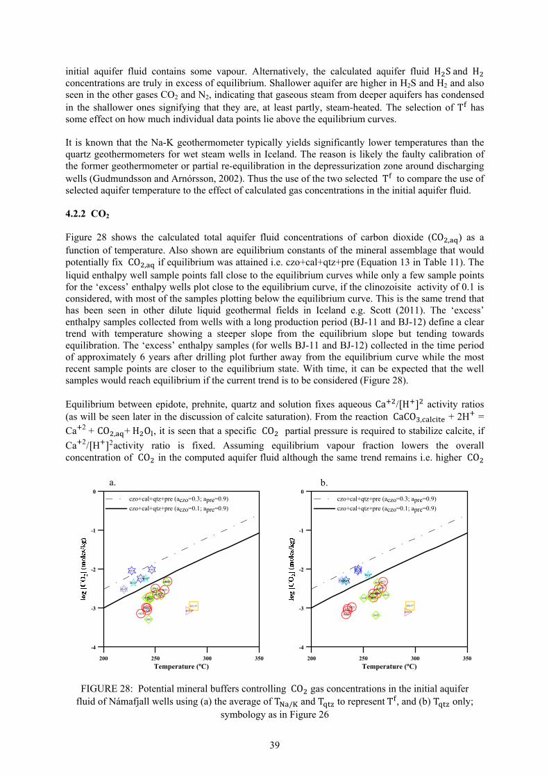
39
initial aquifer fluid contains some vapour. Alternatively, the calculated aquifer fluid H S and H concentrations are truly in excess of equilibrium. Shallower aquifer are higher in H2S and H2 and also seen in the other gases CO2 and N2, indicating that gaseous steam from deeper aquifers has condensed in the shallower ones signifying that they are, at least partly, steam-heated. The selection of T has some effect on how much individual data points lie above the equilibrium curves. It is known that the Na-K geothermometer typically yields significantly lower temperatures than the quartz geothermometers for wet steam wells in Iceland. The reason is likely the faulty calibration of the former geothermometer or partial re-equilibration in the depressurization zone around discharging wells (Gudmundsson and Arnórsson, 2002). Thus the use of the two selected T to compare the use of selected aquifer temperature to the effect of calculated gas concentrations in the initial aquifer fluid. 4.2.2 CO2
Figure 28 shows the calculated total aquifer fluid concentrations of carbon dioxide (CO , ) as a function of temperature. Also shown are equilibrium constants of the mineral assemblage that would potentially fix CO , if equilibrium was attained i.e. czo+cal+qtz+pre (Equation 13 in Table 11). The liquid enthalpy well sample points fall close to the equilibrium curves while only a few sample points for the ‘excess’ enthalpy wells plot close to the equilibrium curve, if the clinozoisite activity of 0.1 is considered, with most of the samples plotting below the equilibrium curve. This is the same trend that has been seen in other dilute liquid geothermal fields in Iceland e.g. Scott (2011). The ‘excess’ enthalpy samples collected from wells with a long production period (BJ-11 and BJ-12) define a clear trend with temperature showing a steeper slope from the equilibrium slope but tending towards equilibration. The ‘excess’ enthalpy samples (for wells BJ-11 and BJ-12) collected in the time period of approximately 6 years after drilling plot further away from the equilibrium curve while the most recent sample points are closer to the equilibrium state. With time, it can be expected that the well samples would reach equilibrium if the current trend is to be considered (Figure 28). Equilibrium between epidote, prehnite, quartz and solution fixes aqueous Ca /[H ] activity ratios (as will be seen later in the discussion of calcite saturation). From the reaction CaCO , + 2H =
Ca 2 + CO , + H O , it is seen that a specific CO partial pressure is required to stabilize calcite, if
Ca 2/[H ]2activity ratio is fixed. Assuming equilibrium vapour fraction lowers the overall concentration of CO in the computed aquifer fluid although the same trend remains i.e. higher CO
FIGURE 28: Potential mineral buffers controlling CO gas concentrations in the initial aquifer fluid of Námafjall wells using (a) the average of T / and T to represent T , and (b) T only;
symbology as in Figure 26
a.
200 250 300 350
Temperature (oC)
-4
-3
-2
-1
0
4036
1014
1012
4034*
4008*4033
4059 4035
401340244022
103410221050
1024
4034
4013
4010103310211038
1005
0551*
0311*
0343*
czo+cal+qtz+pre (aczo=0.3; apre=0.9)
czo+cal+qtz+pre (aczo=0.1; apre=0.9)
b.
200 250 300 350
Temperature (oC)
-4
-3
-2
-1
0
4036
1014
1012
4034*
4008*
4033
40594035
401340244022
10341022
10501024
4034
40134010
103310211038
10050551*
0311*
0343*
czo+cal+qtz+pre (aczo=0.3; apre=0.9)
czo+cal+qtz+pre (aczo=0.1; apre=0.9)

40
in the liquid enthalpy wells as compared to the excess enthalpy wells. CO is affected by supply from source (magma) but also by condensation of steam in relatively shallow sub-boiling aquifers (liquid enthalpy wells). Considering the higher concentration of dissolved acidic gases like CO (which is also shown by the H S and H concentration) in the shallower aquifer wells than the deeper aquifers, it can be suggested that the fluids feeding the aquifers in the liquid enthalpy wells are steam heated waters with the excess enthalpy wells showing degassed aquifer fluid. 4.3 Mineral-solute equilibria If the aqueous concentrations of H S, H and CO are controlled by equilibria with particular mineral assemblages, then the individual minerals in these assemblages should be in equilibrium with the solution. Dissolution reactions of the hydrothermal minerals considered and their corresponding log K-temperature equations are listed in Table 10. For each reaction, departure from equilibrium is expressed as saturation index. The saturation index (SI) is defined as
SI = logQ
K [4.3]
where Q represents activity product of a mineral dissolution reaction and K the equilibrium constant. The activity product (Q) for a mineral or a mineral assemblage is given by
Q = Πiaivi [4.4]
Where Q is the product of all species activities, ai, each raised to the power of its stoichiometric coefficient, vi, which is negative for reactants and positive for products. The activities of aqueous species were obtained with the aid of the WATCH 2.1 program. The activity of water was assumed to be unity. Mineral solid solutions are taken to be ideal. Thus, the activity of end-members of solid solutions were taken to be proportional to their mole fraction raised to the power of the number of exchangeable sites in the crystal lattice, i.e. ai = Xi
n, where X is the mole fraction, ai the activity of the subscribed species and n the number of exchangeable sites. Effect of pH on equilibrium state of aquifer fluid The measured pH of samples affects the calculated initial aquifer pH. For all samples used for this study, pH was measured sometime after the sample was collected and after silica in solution in excess of amorphous silica solubility had polymerized. Precise and immediate onsite measurement of pH of water samples is important for reliable assessment of the state of mineral-solute equilibria in the aquifer and not only for minerals with pH-dependent solubility (e.g. calcite and wollastonite) but also for any mineral–gas equilibria involving CO , and H2Saq because the aquifer water pH affects the relative concentrations of the carbonate and sulphide-bearing species. Measurement of pH sometime after collection appears to be the common practice worldwide, and such measurement may give faulty pH value because silica polymerization may change the water pH depending on what the initial pH was before onset of polymerization (Karingithi et al., 2010). Arnórsson (2000) indicates that the dissociation constant of aqueous silica (silicic acid) changes very much with temperature below 100°C. Silica polymerization changes the pH of water samples by removing the monomeric silica (weak acid) from solution therefore increases pH and by forming oligomers that decrease pH because oligomers are stronger acids than monomers (Tossell and Sahai, 2000). Silica polymerization, at least when pH value is above 9, will cause an increase of the sample value due to the fact that removal of silica monomers dominate the pH change over oligomer formation and at this high pH a significant fraction of the dissolved silica is ionized. The measured pH of the samples is very significant during the WATCH speciation calculations. WATCH initially calculates and sums up the concentrations of all conjugate anions of all acids and OH-bearing species at the temperature at which the pH was measured. This sum (A ) is taken to be constant at all temperatures. The pH at any other temperature is retrieved by iteration until the derived pH satisfies both the value of A and all the dissociation constants for the acids and the OH-bearing species.
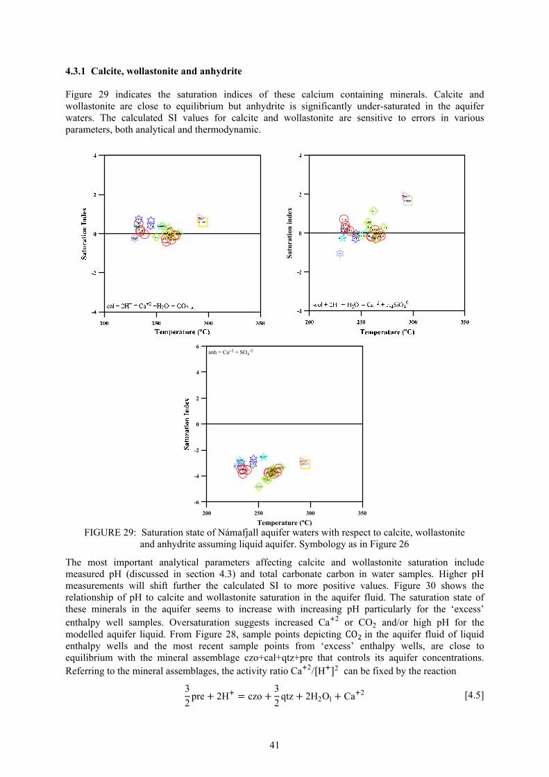
41
4.3.1 Calcite, wollastonite and anhydrite Figure 29 indicates the saturation indices of these calcium containing minerals. Calcite and wollastonite are close to equilibrium but anhydrite is significantly under-saturated in the aquifer waters. The calculated SI values for calcite and wollastonite are sensitive to errors in various parameters, both analytical and thermodynamic.
The most important analytical parameters affecting calcite and wollastonite saturation include measured pH (discussed in section 4.3) and total carbonate carbon in water samples. Higher pH measurements will shift further the calculated SI to more positive values. Figure 30 shows the relationship of pH to calcite and wollastonite saturation in the aquifer fluid. The saturation state of these minerals in the aquifer seems to increase with increasing pH particularly for the ‘excess’ enthalpy well samples. Oversaturation suggests increased Ca 2 or CO2 and/or high pH for the modelled aquifer liquid. From Figure 28, sample points depicting CO in the aquifer fluid of liquid enthalpy wells and the most recent sample points from ‘excess’ enthalpy wells, are close to equilibrium with the mineral assemblage czo+cal+qtz+pre that controls its aquifer concentrations. Referring to the mineral assemblages, the activity ratio Ca 2/[H ]2 can be fixed by the reaction
3
2pre + 2H = czo + 3
2qtz + 2H2Ol + Ca 2 [4.5]
FIGURE 29: Saturation state of Námafjall aquifer waters with respect to calcite, wollastonite
and anhydrite assuming liquid aquifer. Symbology as in Figure 26
Sat
urat
ion
inde
x
200 250 300 350
Temperature (oC)
-6
-4
-2
0
2
4
6
4036
1014 10124034*
4008*
40334059
4035401340244022
1034102210501024 4034
4013 4010
10331021
1038
1005
0551*0311*
0343*
anh = Ca+2 + SO4-2
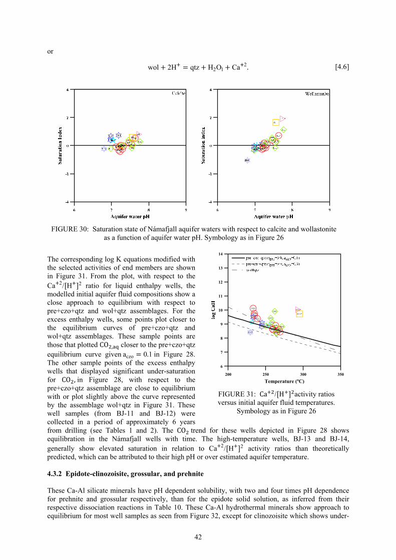
42
or
wol + 2H = qtz + H2Ol + Ca 2. [4.6]
The corresponding log K equations modified with the selected activities of end members are shown in Figure 31. From the plot, with respect to the Ca 2/[H ]2 ratio for liquid enthalpy wells, the modelled initial aquifer fluid compositions show a close approach to equilibrium with respect to pre+czo+qtz and wol+qtz assemblages. For the excess enthalpy wells, some points plot closer to the equilibrium curves of pre+czo+qtz and wol+qtz assemblages. These sample points are those that plotted CO , closer to the pre+czo+qtz equilibrium curve given aczo = 0.1 in Figure 28. The other sample points of the excess enthalpy wells that displayed significant under-saturation for CO , in Figure 28, with respect to the pre+czo+qtz assemblage are close to equilibrium with or plot slightly above the curve represented by the assemblage wol+qtz in Figure 31. These well samples (from BJ-11 and BJ-12) were collected in a period of approximately 6 years from drilling (see Tables 1 and 2). The CO trend for these wells depicted in Figure 28 shows equilibration in the Námafjall wells with time. The high-temperature wells, BJ-13 and BJ-14, generally show elevated saturation in relation to Ca 2/[H ]2 activity ratios than theoretically predicted, which can be attributed to their high pH or over estimated aquifer temperature. 4.3.2 Epidote-clinozoisite, grossular, and prehnite These Ca-Al silicate minerals have pH dependent solubility, with two and four times pH dependence for prehnite and grossular respectively, than for the epidote solid solution, as inferred from their respective dissociation reactions in Table 10. These Ca-Al hydrothermal minerals show approach to equilibrium for most well samples as seen from Figure 32, except for clinozoisite which shows under-
FIGURE 30: Saturation state of Námafjall aquifer waters with respect to calcite and wollastonite
as a function of aquifer water pH. Symbology as in Figure 26
FIGURE 31: Ca /[H ] activity ratios versus initial aquifer fluid temperatures.
Symbology as in Figure 26
200 250 300 350
Temperature (oC)
6
7
8
9
10
11
12
13
14
4036
1014
1012
4034*
4008*
40334059
4035
4013
4024
4022
1034
1022
1050
1024
4034
40134010
1033
1021
1038
10050551*
0311*
0343*
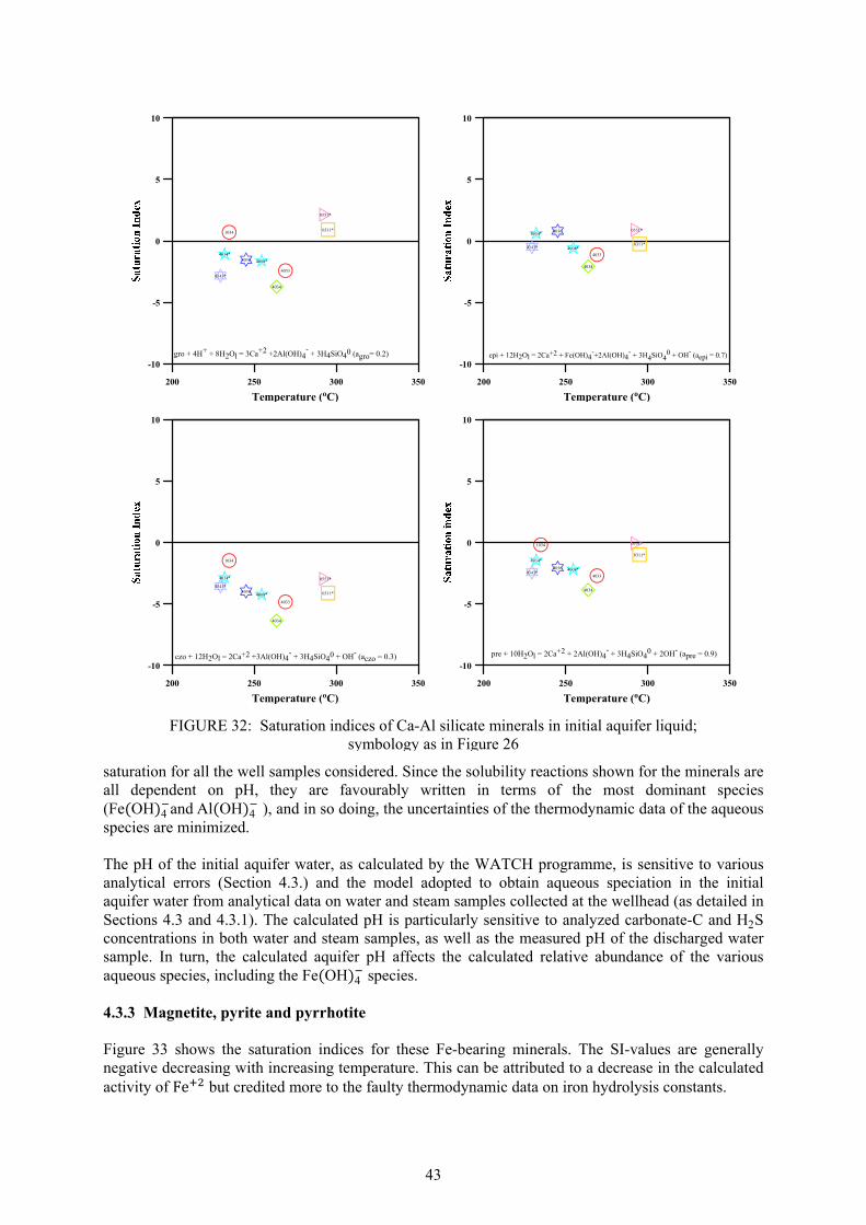
43
saturation for all the well samples considered. Since the solubility reactions shown for the minerals are all dependent on pH, they are favourably written in terms of the most dominant species (Fe(OH)4 and Al(OH)4 ), and in so doing, the uncertainties of the thermodynamic data of the aqueous species are minimized. The pH of the initial aquifer water, as calculated by the WATCH programme, is sensitive to various analytical errors (Section 4.3.) and the model adopted to obtain aqueous speciation in the initial aquifer water from analytical data on water and steam samples collected at the wellhead (as detailed in Sections 4.3 and 4.3.1). The calculated pH is particularly sensitive to analyzed carbonate-C and H2S concentrations in both water and steam samples, as well as the measured pH of the discharged water sample. In turn, the calculated aquifer pH affects the calculated relative abundance of the various aqueous species, including the Fe(OH)4 species. 4.3.3 Magnetite, pyrite and pyrrhotite Figure 33 shows the saturation indices for these Fe-bearing minerals. The SI-values are generally negative decreasing with increasing temperature. This can be attributed to a decrease in the calculated activity of Fe but credited more to the faulty thermodynamic data on iron hydrolysis constants.
FIGURE 32: Saturation indices of Ca-Al silicate minerals in initial aquifer liquid;
symbology as in Figure 26
200 250 300 350
Temperature (oC)
-10
-5
0
5
10
40364034*
4008*
4033
1034
4034
0551*
0311*
0343*
gro + 4H+ + 8H2Ol = 3Ca+2 +2Al(OH)4-
+ 3H4SiO40 (agro= 0.2)
200 250 300 350
Temperature (oC)
-10
-5
0
5
10
40364034*
4008*
4033
4034
0551*
0311*0343*
epi + 12H2Ol = 2Ca+2 + Fe(OH)4-+2Al(OH)4
- + 3H4SiO40 + OH- (aepi = 0.7)
200 250 300 350
Temperature (oC)
-10
-5
0
5
10
4036
4034*
4008*
4033
1034
4034
0551*
0311*
0343*
czo + 12H2Ol = 2Ca+2 +3Al(OH)4- + 3H4SiO40 + OH- (aczo = 0.3)
200 250 300 350
Temperature (oC)
-10
-5
0
5
10
4036
4034*
4008*
4033
1034
4034
0551*
0311*
0343*
pre + 10H2Ol = 2Ca+2 + 2Al(OH)4- + 3H4SiO4
0 + 2OH- (apre = 0.9)
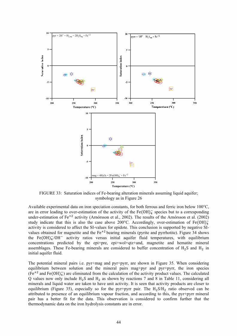
44
Available experimental data on iron speciation constants, for both ferrous and ferric iron below 100°C, are in error leading to over-estimation of the activity of the Fe(OH) species but to a corresponding under-estimation of Fe activity (Arnórsson et al., 2002). The results of the Arnórsson et al. (2002) study indicate that this is also the case above 200°C. Accordingly, over-estimation of Fe(OH) activity is considered to affect the SI-values for epidote. This conclusion is supported by negative SI-values obtained for magnetite and the Fe bearing minerals (pyrite and pyrrhotite). Figure 34 shows the Fe(OH) /OH activity ratios versus initial aquifer fluid temperatures, with equilibrium concentrations predicted by the epi+pre, epi+wol+qtz+and, magnetite and hematite mineral assemblages. These Fe-bearing minerals are considered to buffer concentration of H S and H in initial aquifer fluid. The potential mineral pairs i.e. pyr+mag and pyr+pyrr, are shown in Figure 35. When considering equilibrium between solution and the mineral pairs mag+pyr and pyr+pyrr, the iron species (Fe and Fe(OH) ) are eliminated from the calculation of the activity product values. The calculated Q values now only include H S and H as shown by reactions 7 and 8 in Table 11, considering all minerals and liquid water are taken to have unit activity. It is seen that activity products are closer to equilibrium (Figure 35), especially so for the pyr+pyrr pair. The H S/H ratio observed can be attributed to presence of an equilibrium vapour fraction, and according to this, the pyr+pyrr mineral pair has a better fit for the data. This observation is considered to confirm further that the thermodynamic data on the iron hydrolysis constants are in error.
FIGURE 33: Saturation indices of Fe-bearing alteration minerals assuming liquid aquifer; symbology as in Figure 26
200 250 300 350
Temperature (oC)
-10
-5
0
5
10
40364034*
4008*
40334059
40354013
402440224034 4010
0551*0311*
0343*
pyr + 2H+ + H2,aq = 2H2Saq + Fe+2
Satu
rati
onin
dex
200 250 300 350
Temperature (oC)
-10
-5
0
5
10
4036
4034*
4008*4033
4059
4035401340244022
4034
4010
0551*
0311*
0343*
mag + 4H2Ol = 2Fe(OH)4- + Fe+2
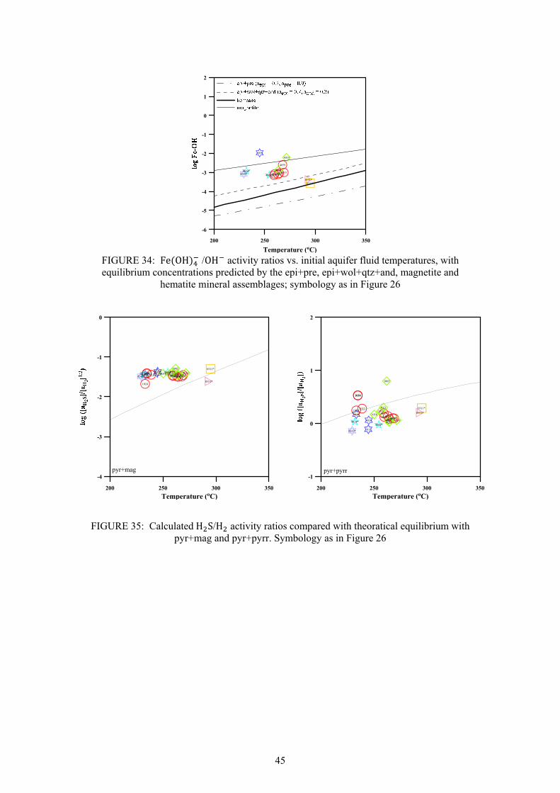
45
FIGURE 35: Calculated H S/H activity ratios compared with theoratical equilibrium with pyr+mag and pyr+pyrr. Symbology as in Figure 26
200 250 300 350
Temperature (oC)
-4
-3
-2
-1
0
40361014
10124034*4008*
403340594035401340244022103410221050
1024
4034401340101033
10211038
1005
0551*
0311*
0343*
pyr+mag
200 250 300 350
Temperature (oC)
-1
0
1
2
4036
1014
1012
4034*4008*
403340594035
401340244022
1034
1022
1050
1024
40344013
4010
10331021
1038
1005
0551*
0311*
0343*
pyr+pyrr
FIGURE 34: Fe(OH) /OH activity ratios vs. initial aquifer fluid temperatures, with equilibrium concentrations predicted by the epi+pre, epi+wol+qtz+and, magnetite and
hematite mineral assemblages; symbology as in Figure 26
200 250 300 350
Temperature (oC)
-6
-5
-4
-3
-2
-1
0
1
2
4036
4034*
4008*4033
4059
4035401340244022
4034
4010
0551*0311*
0343*
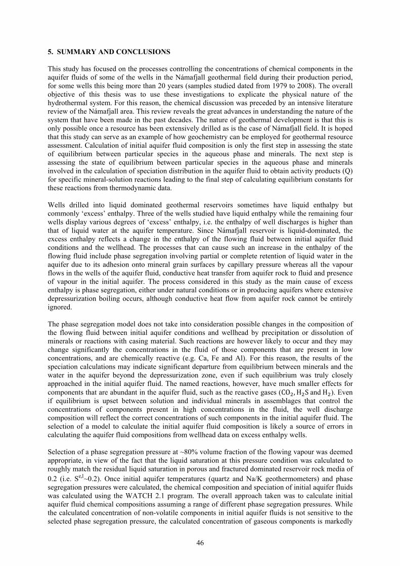
46
5. SUMMARY AND CONCLUSIONS This study has focused on the processes controlling the concentrations of chemical components in the aquifer fluids of some of the wells in the Námafjall geothermal field during their production period, for some wells this being more than 20 years (samples studied dated from 1979 to 2008). The overall objective of this thesis was to use these investigations to explicate the physical nature of the hydrothermal system. For this reason, the chemical discussion was preceded by an intensive literature review of the Námafjall area. This review reveals the great advances in understanding the nature of the system that have been made in the past decades. The nature of geothermal development is that this is only possible once a resource has been extensively drilled as is the case of Námafjall field. It is hoped that this study can serve as an example of how geochemistry can be employed for geothermal resource assessment. Calculation of initial aquifer fluid composition is only the first step in assessing the state of equilibrium between particular species in the aqueous phase and minerals. The next step is assessing the state of equilibrium between particular species in the aqueous phase and minerals involved in the calculation of speciation distribution in the aquifer fluid to obtain activity products (Q) for specific mineral-solution reactions leading to the final step of calculating equilibrium constants for these reactions from thermodynamic data. Wells drilled into liquid dominated geothermal reservoirs sometimes have liquid enthalpy but commonly ‘excess’ enthalpy. Three of the wells studied have liquid enthalpy while the remaining four wells display various degrees of ‘excess’ enthalpy, i.e. the enthalpy of well discharges is higher than that of liquid water at the aquifer temperature. Since Námafjall reservoir is liquid-dominated, the excess enthalpy reflects a change in the enthalpy of the flowing fluid between initial aquifer fluid conditions and the wellhead. The processes that can cause such an increase in the enthalpy of the flowing fluid include phase segregation involving partial or complete retention of liquid water in the aquifer due to its adhesion onto mineral grain surfaces by capillary pressure whereas all the vapour flows in the wells of the aquifer fluid, conductive heat transfer from aquifer rock to fluid and presence of vapour in the initial aquifer. The process considered in this study as the main cause of excess enthalpy is phase segregation, either under natural conditions or in producing aquifers where extensive depressurization boiling occurs, although conductive heat flow from aquifer rock cannot be entirely ignored. The phase segregation model does not take into consideration possible changes in the composition of the flowing fluid between initial aquifer conditions and wellhead by precipitation or dissolution of minerals or reactions with casing material. Such reactions are however likely to occur and they may change significantly the concentrations in the fluid of those components that are present in low concentrations, and are chemically reactive (e.g. Ca, Fe and Al). For this reason, the results of the speciation calculations may indicate significant departure from equilibrium between minerals and the water in the aquifer beyond the depressurization zone, even if such equilibrium was truly closely approached in the initial aquifer fluid. The named reactions, however, have much smaller effects for components that are abundant in the aquifer fluid, such as the reactive gases (CO , H S and H ). Even if equilibrium is upset between solution and individual minerals in assemblages that control the concentrations of components present in high concentrations in the fluid, the well discharge composition will reflect the correct concentrations of such components in the initial aquifer fluid. The selection of a model to calculate the initial aquifer fluid composition is likely a source of errors in calculating the aquifer fluid compositions from wellhead data on excess enthalpy wells. Selection of a phase segregation pressure at ~80% volume fraction of the flowing vapour was deemed appropriate, in view of the fact that the liquid saturation at this pressure condition was calculated to roughly match the residual liquid saturation in porous and fractured dominated reservoir rock media of 0.2 (i.e. Se,l~0.2). Once initial aquifer temperatures (quartz and Na/K geothermometers) and phase segregation pressures were calculated, the chemical composition and speciation of initial aquifer fluids was calculated using the WATCH 2.1 program. The overall approach taken was to calculate initial aquifer fluid chemical compositions assuming a range of different phase segregation pressures. While the calculated concentration of non-volatile components in initial aquifer fluids is not sensitive to the selected phase segregation pressure, the calculated concentration of gaseous components is markedly
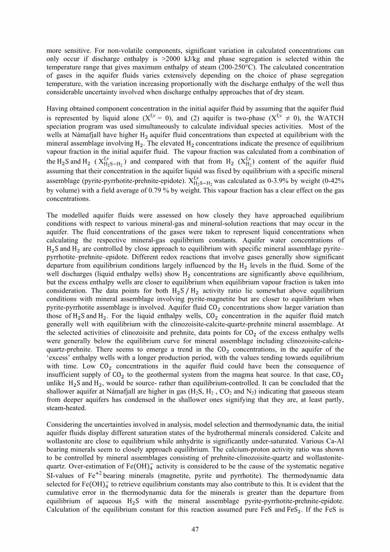
47
more sensitive. For non-volatile components, significant variation in calculated concentrations can only occur if discharge enthalpy is >2000 kJ/kg and phase segregation is selected within the temperature range that gives maximum enthalpy of steam (200-250°C). The calculated concentration of gases in the aquifer fluids varies extensively depending on the choice of phase segregation temperature, with the variation increasing proportionally with the discharge enthalpy of the well thus considerable uncertainty involved when discharge enthalpy approaches that of dry steam. Having obtained component concentration in the initial aquifer fluid by assuming that the aquifer fluid is represented by liquid alone (Xf,v = 0), and (2) aquifer is two-phase (Xf,v ≠ 0), the WATCH speciation program was used simultaneously to calculate individual species activities. Most of the wells at Námafjall have higher H aquifer fluid concentrations than expected at equilibrium with the mineral assemblage involving H . The elevated H concentrations indicate the presence of equilibrium vapour fraction in the initial aquifer fluid. The vapour fraction was calculated from a combination of the H S and H ( XH2S H2 f,v ) and compared with that from H (XH2
f,v ) content of the aquifer fluid assuming that their concentration in the aquifer liquid was fixed by equilibrium with a specific mineral assemblage (pyrite-pyrrhotite-prehnite-epidote). XH2S H2 f,v was calculated as 0-3.9% by weight (0-42% by volume) with a field average of 0.79 % by weight. This vapour fraction has a clear effect on the gas concentrations. The modelled aquifer fluids were assessed on how closely they have approached equilibrium conditions with respect to various mineral-gas and mineral-solution reactions that may occur in the aquifer. The fluid concentrations of the gases were taken to represent liquid concentrations when calculating the respective mineral-gas equilibrium constants. Aquifer water concentrations of H S and H are controlled by close approach to equilibrium with specific mineral assemblage pyrite–pyrrhotite–prehnite–epidote. Different redox reactions that involve gases generally show significant departure from equilibrium conditions largely influenced by the H levels in the fluid. Some of the well discharges (liquid enthalpy wells) show H concentrations are significantly above equilibrium, but the excess enthalpy wells are closer to equilibrium when equilibrium vapour fraction is taken into consideration. The data points for both H S / H activity ratio lie somewhat above equilibrium conditions with mineral assemblage involving pyrite-magnetite but are closer to equilibrium when pyrite-pyrrhotite assemblage is involved. Aquifer fluid CO concentrations show larger variation than those of H S and H . For the liquid enthalpy wells, CO concentration in the aquifer fluid match generally well with equilibrium with the clinozoisite-calcite-quartz-prehnite mineral assemblage. At the selected activities of clinozoisite and prehnite, data points for CO of the excess enthalpy wells were generally below the equilibrium curve for mineral assemblage including clinozoisite-calcite-quartz-prehnite. There seems to emerge a trend in the CO concentrations, in the aquifer of the ‘excess’ enthalpy wells with a longer production period, with the values tending towards equilibrium with time. Low CO concentrations in the aquifer fluid could have been the consequence of insufficient supply of CO to the geothermal system from the magma heat source. In that case, CO unlike H S and H , would be source- rather than equilibrium-controlled. It can be concluded that the shallower aquifer at Námafjall are higher in gas (H2S, H2 , CO2 and N2) indicating that gaseous steam from deeper aquifers has condensed in the shallower ones signifying that they are, at least partly, steam-heated. Considering the uncertainties involved in analysis, model selection and thermodynamic data, the initial aquifer fluids display different saturation states of the hydrothermal minerals considered. Calcite and wollastonite are close to equilibrium while anhydrite is significantly under-saturated. Various Ca-Al bearing minerals seem to closely approach equilibrium. The calcium-proton activity ratio was shown to be controlled by mineral assemblages consisting of prehnite-clinozoisite-quartz and wollastonite-quartz. Over-estimation of Fe(OH)4 activity is considered to be the cause of the systematic negative SI-values of Fe 2 bearing minerals (magnetite, pyrite and pyrrhotite). The thermodynamic data selected for Fe(OH)4 to retrieve equilibrium constants may also contribute to this. It is evident that the cumulative error in the thermodynamic data for the minerals is greater than the departure from equilibrium of aqueous H S with the mineral assemblage pyrite-pyrrhotite-prehnite-epidote. Calculation of the equilibrium constant for this reaction assumed pure FeS and FeS . If the FeS is

48
deficient in iron, the equilibrium curve is shifted to lower values, as does the presence of S 2 in FeS . Sulfide mineral analysis is missing for quantitative estimation of the effect of the iron-sulfide mineral composition on the equilibrium constant. In addition, the uncertainties on the thermodynamic data on these mineral, as given by Robie and Hemingway (1995) may produce an error as high as 0.3 log mol/kg on the equilibrium H S concentration, in addition to the error produced by the silicate minerals, epidote and prehnite.
49
REFERENCES Ármannsson, H., 2011: EIA – example from Bjarnaflag in Iceland. University of Iceland, geothermal resources (JAR218), lecture notes. Ármannsson, H., 2005: Monitoring the effect of geothermal effluent from the Krafla and Bjarnarflag power plants on groundwater in the Lake Mývatn area, Iceland, with particular reference to natural. Proceedings World Geothermal Congress 2005 Antalya, Turkey, 8 pp. Ármannsson, H., 1993: The geothermal system in Námafjall. Geochemical investigation. Orkustofnun, Reykjavik, report 93053/JHD-29B, 30 pp. Ármannsson, H., Benjamínsson, J., Jeffrey, A.W.A., 1989: Gas changes in the Krafla geothermal system, Iceland. Chem. Geol. 76, 175–196. Ármannsson, H., Gudmundsson, Á., Steingrímsson, B.S., 1987: Exploration and development of the Krafla geothermal area. Jökull 37, 13–30. Ármannsson, H. and Ólafsson, M. 2007: Geothermal sampling and analysis. Presented at the Short Course II on “Surface Exploration for Geothermal Resources”, organized by UNU-GTP and KenGen, at Lake Naivasha, Kenya, 2-17 November. Ármannsson, H. and Ólafsson, M. 2006: Collection of geothermal fluids for chemical analysis. ÍSOR, Reykjavík, report ÍSOR-2006/016, 17 pp. Árnason, J. G., Bird, D. K., 1992: Formation of zoned epidote in hydrothermal systems. In: Water-Rock Interaction 7-2, 1473-1476. Árnason, K., Karlsdóttir, R., Eysteinsson, H., Flóvenz, Ó., and Gudlaugsson, S., 2000: The resistivity structure of high-temperature geothermal systems in Iceland. Proceedings of the World Geothermal Congress 2000, Kyushu-Tohoku, Japan, 923-928. Angcoy, E.C. Jr., 2010: Geochemical modelling of the high temperature Mahanagdong geothermal field, Letye, Philippines. University of Iceland, MSc Thesis, UNU-GTP, Iceland, report 1, 71 pp. Arnórsson, S. (ed), 2000: Isotopic and chemical techniques in geothermal exploration, development and use. Sampling methods, data handling and interpretation. International Atomic Energy Agency, Vienna, 351 pp. Arnórsson, S., 1995: Geothermal systems in Iceland: Structure and conceptual models. 1. High-temperature areas. Geothermics, 24, 561-602. Arnórsson, S., Angcoy, Jr., E.C., Bjarnason, J.Ö., Giroud, N., Gunnarsson, I., Kaasalainen, H., Karingithi, C., and Stefánsson, A., 2010: Gas chemistry of volcanic geothermal systems. Proceedings World Geothermal Congress 2010, Bali, Indonesia. Arnórsson, S., Björnsson, S., Muna, Z.W., Bwire-Ojiambo, S., 1990: The use of gas chemistry to evaluate boiling processes and initial steam fractions in geothermal reservoirs with an example from the Olkaria field, Kenya. Geothermics, 19, 497–514. Arnórsson, S., Fridriksson, Th., Gunnarsson, I., 1998: Gas chemistry of the Krafla geothermal field, Iceland. Water Rock Interaction, Proc. Int. Symp. Auckland, New Zealand, 613-616. Arnórsson, S. and Gunnlaugsson, E., 1985: New gas geothermometers for geothermal exploration - calibration and application. Geochim Cosmochim Acta, 49, 1307-1325.

50
Arnórsson, S., Gunnlaugsson, E., and Svavarsson, H., 1983: The chemistry of geothermal waters in Iceland. II. Mineral equilibria and independent variables controlling water compositions. Geochimica et Cosmochimica Acta, 47, 547-566. Arnórsson, S., Sigurdsson, S., and Grönvold, K., 1978: Aquifer chemistry of four geothermal areas in Iceland. Geochem. Cosmocim. Acta, 42, 523-536. Arnórsson, S., Sigurdsson, S., and Svavarsson, H., 1982: The chemistry of geothermal waters in Iceland. I. Calculations of aqueous speciation from 0° to 370°C. Geochim. Cosmochim. Acta, 46, 1513-1532. Arnórsson, S. and Stefánsson, A., 2005: Wet-steam well discharges. II. Assessment of aquifer fluid compositions. World Geothermal Congress, Antalya, Turkey. Arnórsson, S., and Stefánsson, A., 1999: Assessment of feldspar solubility constants in water in the range 0 to 350 °C at vapour saturation pressures. Amer. J. Sci., 299, 173-209. Arnórsson, S., Stefánsson, A., and Bjarnason, J.Ö., 2007: Fluid-fluid interaction in geothermal systems. Reviews in Mineralogy & Geochemistry, 65, 229-312. Bird, D. K., Spieler, A. R., 2004: Epidote in geothermal systems. Reviews in Mineralogy & Geochemistry, 56, 235-300. Bischoff, J.L. and Rosenbauer, R.J., 1989: Salinity variations in submarine hydrothermal systems by double diffusive convection. Journal of Geology, 7, 613-623. Bjarnason, J.Ö., 1994: The speciation program WATCH, version 2.1. Orkustofnun, Reykjavík, 7 pp. Bödvarsson, G.S., Benson, S.M., Sigurdsson, Ó., Stefánsson, V., Elíasson, E.T., 1984a: The Krafla geothermal field, Iceland. 1. Analysis of well test data. Water Resour. Res., 20, 1515-1530. Bödvarsson, G.S., Pruess, K., Stefánsson, V., Elíasson, E.T., 1984b: The Krafla geothermal field Iceland 2. The natural state of the system. Water Resour. Res., 20, 1531–1544. Brandsdóttir, B. and Einarsson, P. 1979: Seismic activity associated with September 1977 deflation of the Krafla central volcano in NE Iceland. J. Volcanol. Geotherm. Res., 6, 197-212. Chen, C.Y., and Horne, R.N., 2006: Two-phase flow in rough-walled fractures: Experiments and a flow structure model. Water Resources Research, 42. Chen, C.Y., Horne, R.N., and Fourar, M., 2004: Experimental study of two-phase flow structure effects on relative permeabilities in a fracture. 29th Workshop on Geothermal Reservoir Engineering, Stanford University, Stanford, CA. Corey, A.T., 1957: Measurement of water and air permeabilities in unsaturated soil. Soil Sci. Soc. Am. Proc., 21, 7–10. D’Amore, F., and Celati, R., 1983: Methodology for calculating steam quality in geothermal reservoirs. Geothermics 12, 129-140 D’Amore, F., and Truesdell, A.H., 1985: Calculation of geothermal reservoir temperatures and steam fractions from gas compositions. Geotherm. Res. Council, Trans., 9, 305-310 Darling, G., Ármannsson, H., 1989: Stable isotopic aspects of fluid flow in the Krafla, Námafjall and Theistareykir geothermal systems of northeast Iceland. Chem., Geol. 79, 197–213.
51
De Zeeuw, E. and Gíslason, G., 1988: The effect of volcanic activity on the groundwater system in the Námafjall geothermal area, NE-Iceland. Orkustofnun, Reykjavík, report OS-88042/JHD-07, 39 pp. Diakonov, I. I., Schott, J., Martin, F., Harrichourry, J. C., Escalier, J., 1999: Iron(III) solubility and speciation in aqueous solutions. Experimental study and modelling: Part 1. Hematite solubility from 60 to 300 degrees C in NaOH-NaCl solutions and thermodynamic properties of Fe(OH)4,aq. Geochim. Cosmochim. Acta, 63, 2247-2261. Fernández-Prini, R., Alvarez, J. L., Harvey, A. H., 2003: Henry's constants and vapour-liquid distribution constants for gaseous solutes in H2O and D2O at high temperatures. Journal of Physical and Chemical Reference Data, 32-2, 903-916. Flóvenz, Ó.G., 2011: Resistivity, magma and geothermal systems. University of Iceland, Geothermal Resources (JAR218), lecture notes. Flóvenz, Ó.G., Spangenberg, E., Kulenkamp, J., Árnason, K., Karlsdóttir, R., Huenges, E., 2005: The role of electrical interface conduction in geothermal exploration. Proceedings World Geothermal Congress 2005 Antalya, Turkey, 24-29. Fournier, R.O., and Potter, R.W.II, 1982: A revised and expanded silica (quartz) geothermometers. Geotherm. Res. Council, Bull., 11, 3-9. Frauke, W., Fridriksson, Th., and Ármannsson, H., 2008: CO2 fixation by calcite in high-temperature geothermal systems in Iceland. ÍSOR, Reykjavík, report 2008/003, 68 pp. Georgsson, L.S., 2010. Geophysical methods used in geothermal exploration. Presented at “Short Course V on Exploration for Geothermal Resources”, organized by UNU-GTP, GDC and KenGen, at Lake Bogoria and Lake Naivasha, Kenya, Oct. 29 – Nov. 19, 2010. Georgsson, L.S. and Karlsdóttir R., 2009: Resistivity methods - DC and TEM with examples and comparison from the Reykjanes peninsula and Öxarfjördur, Iceland. Presented at “Short Course on Surface Exploration for Geothermal Resources”, organized by UNU-GTP and LaGeo, in Ahuachapan and Santa Tecla, El Salvador, 17-30. Giggenbach, W.F., 1980: Geothermal gas equilibria. Geochim. Cosmochim Acta, 44, 2021-2032. Giroud N., 2008: A chemical study of arsenic, boron and gases in high-temperature geothermal fluids in Iceland. University of Iceland, Reykjavík, PhD thesis, 128 pp. Glover, R.B., Lovelock, B., and Ruaya, J.R., 1981: A novel way of using gas and enthalpy. New Zealand Geothermal Workshop, Auckland, New Zealand, 163-169. Gudmundsson, Á. 1993: The alteration formation temperature in the geothermal system in Bjarnarflag. Orkustofnun, Reykjavík, report OS-93065/JHD-31 B (in Icelandic), 21 pp. Gudmundsson, B.T. and Arnórsson, S., 2005: Secondary mineral-fluid equilibria in the Krafla and Namafjall geothermal systems, Iceland. Appl. Geochem., 20, 1607-1625. Gudmundsson, B., and Arnórsson, S., 2002: Geochemical monitoring of the Krafla and Námafjall geothermal areas, N-Iceland. Geothermics, 31, 195-243. Gudmundsson, M.T., Larsen, G., Höskuldsson, Á. and Gylfason, Á.G., 2008: Volcanic hazards in Iceland. Jökull, 58, 251-268.
52
Gudmundsson, Á., Mortensen, A.K., Hjartarson, A., Karlsdóttir, R. and Ármannsson, H. 2010: Exploration and utilization of the Námafjall high temperature area in N-Iceland. Proceedings World Geothermal Congress Bali, Indonesia. Gunnarsson, I., Arnórsson, S., 2000: Amorphous silica solubility and the thermodynamic properties of H4SiO4 degrees in the range of 0 degrees to 350 degrees C at P-sat. Geochim. Cosmochim. Acta, 64-13, 2295-2307. Hauksson, T., and Benjamínsson, J., 1997: Well performance and chemical analysis of water and steam from well discharges. Landsvirkjun - National Power Company, Reykjavík, report (in Icelandic), 70 pp. Hauksson, T., and Benjamínsson, J., 1995: Krafla and Bjarnarflag. Production of wells and chemical composition of fluids from wells and power plant. Landsvirkjun - National Power Company, Reykjavík, report (in Icelandic), 64 pp. Hauksson, T., and Benjamínsson, J., 1989: Krafla and Bjarnarflag. Production of wells and chemical composition of fluids from wells and power plant. Landsvirkjun - National Power Company Reykjavík, report (in Icelandic), 51 pp. Hauksson, T., and Benjamínsson, J., 2000: Krafla and Bjarnarflag. Production of wells and chemical composition of fluids from wells and power plant. National Power Company, report (in Icelandic), 66 pp. Helgeson, H.C., 1967: Thermodynamics of complex dissociation in aqueous solution at elevated temperatures. J. Phys. Chem., 71, 3121-3136. Hersir G.P., and Árnason, K., 2009: Resistivity of rocks. Presented at “Short Course on Surface Exploration for Geothermal Resources”, organized by UNU-GTP and LaGeo, in Ahuachapan and Santa Tecla, El Salvador, 17-30. Hjartarson, A., Sigurdsson Ó., Gudmundsson Á., Ármannsson, H., Karlsdóttir R., 2005: Numerical modeling of the geothermal system in námafjall and response prediction of 30-90 mw electrical generation in Bjarnarflag. ÍSOR, Reykjavík, report ÍSOR 2004/009 (in Icelandic), 123 pp. Hönnun, 2003a: The Bjarnarflag power plant 90 MWe and the 132 kV Bjarnarflag power transmission line 1 in Skútustadahreppur. Environmental Impact Assessment. Landsvirkjun, Reykjavík, report, LV-2003/123, 116 pp. Hönnun, 2003b: The Bjarnarflag power plant up to 90 MWe and the 132 kV Bjarnarflag power transmission line 1 in Skútustadahreppur. Environmental Impact Assessment. Landsvirkjun, Reykjavík, scoping document, LV-2003/052, 46 pp. Hönnun, 2003c: The Bjarnarflag power plant 90 MWe and the 132 kV Bjarnarflag power transmission line 1 in Skútustadahreppur. Environmental Impact Assessment. Landsvirkjun, Reykjavík, LV-2003/123, appendices, 267 pp. Hönnun, 1996: A geothermal power plant at Bjarnarflag. Environmental Impact Assessment. Initial environmental impact assessment for a 2×20 MWe geothermal power plant in Bjarnarflag and a 132 kV high voltage transmission line between the Krafla power plant. Landsvirkjun, Reykjavík, 101 pp. Holland, T. J. B., Powell, R., 1998: An internally consistent thermodynamic data set for phases of petrological interest. Journal of Metamorphic Geology, 16-3, 309-343.
53
Horne, R.N., Satik, C., Mahiya, G., Li., K., Ambuso, W., Tovar, R., Wang, C., and Nassori, N., 2000: Steam-water relative permeability. Proceedings World Geothermal Congress 2000, Kyushu-Tohoku, Japan, 2609-2615. Hreggvidsdóttir, H., 1987: The greenschist to amphibolite facies transition in the Nesjavellir hydrothermal system, Southwest Iceland. University of Stanford, Stanford, MSc thesis. Ingebritsen, S.E., Geiger, S., Hurwitz, S. and Driesner, T., 2010: Numerical simulation of magmatic hydrothermal systems. Reviews of Geophysics, 48, 33 pp. Isabyrie, E., 1994: Borehole geology and hydrothermal alteration in well B-9, Námafjall geothermal field, NE-Iceland. Report 5 in: Geothermal Training in Iceland 1994. UNU-GTP, Iceland, 89-121. Jakobsson, S. P. 1979. Petrology of recent basalts of the Eastern Volcanic Zone, Iceland. Acta Naturalia Islandia, 26, 1-103. Jóhannesson, H. and K. Saemundsson 1998. Geological map of Iceland. Bedrock geology, scale 1:500.000. Nátturufraedistofnun Islands, Reykjavík (2nd edition). Johnson, J. W., Oelkers, E. H., Helgeson, H. C., 1992: SUPCRT92 - A software package for calculating the standard molal thermodynamic properties of minerals, gases, aqueous species, and reactions from 1-bar to 5000-bar and 0-degrees-C to 1000-degrees-C. Computers and Geosciences, 18, 899-947. Karingithi, C. W., Arnórsson, S., and Gronvold, K., 2010: Processes controlling aquifer fluid compositions in the Olkaria geothermal system, Kenya. J. Volcanol. Geoth. Res., 196, 57-76. Karlsdóttir, R., 2002: Námafjall. TEM-resistivity measurements 2001. Orkustofnun, Reykjavík, report OS-2002/057 (in Icelandic), 68 pp. Karlsdóttir, R., 1993: Námafjall. TEM-resistivity measurements 1992. Orkustofnun, Reykjavík, report OS-93022/JHD-12, 34 pp. Kristmannsdóttir, H., 1979: Alteration of basaltic rocks by hydrothermal activity at 100-300°C. In: Mortland, M.M., and Farmer, V.C. (editors), International Clay Conference 1978. Elsevier Scientific Publishing Co., Amsterdam, 359-367. Kristmannsdóttir, H., 1978: Alteration of bedrock in the Krafla geothermal system. Orkustofnun, Reykjavík, report OSJHD 7854 (in Icelandic). Kristmannsdóttir, H. and Ármannsson, H., 2004: Groundwater in the Lake Mývatn area, northern Iceland. Chemistry, Origin and Interaction, Aquatic Ecology, 115-128. Larsen, G., Gronvold, K., and Thorarinsson, S., 1978: Volcanic eruption through a geothermal borehole at Námafjall, Iceland. Nordic Volcanological Institute, Science Institute, Reykjavik, report RH-78-10, 22 pp. Li, K. and Horne, R.N., 2004a: An analytical scaling method for spontaneous imbibitions in gas-water-rock systems. SPEJ, 9-3, 322-329. Li, K. and Horne, R.N., 2004b: Experimental study of gas slippage in two-phase flow. SPEREE, 409-414. Lonker, S. W., Franzson, H., Kristmannsdóttir, H., 1993: Mineral-fluid interactions in the Reykjanes and Svartsengi geothermal systems, Iceland. American Journal of Science, 293, 605-670.
54
Mortensen, A., Egilson, T., Gautason, B., Gunnarsson, H., and Ingólfsson, T., 2008: Bjarnarflag- well BJ-14. 3rd stage: Drilling of production section from 847 m to 2506 m depth. ÍSOR – Iceland GeoSurvey, Reykjavik, report ÍSOR -2008/039 (in Icelandic). Nicholson, H., Condomines, M., Fitton, J.G., Fallick, F.E., Grönvold, K., and Rogers G., 1991: Geochemical and isotopic evidence for crustal assimilation beneath Krafla, Iceland. J. Petrol., 32, 1005-1020. Noorollahi, Y., 2005: Application of GIS and remote sensing in exploration and environmental management of Námafjall geothermal area, N-Iceland. University of Iceland, M.Sc. Thesis, 176 pp. Ólafsson, M., and Kristmannsdóttir, H., 1989: The influence of volcanic activity on groundwater chemistry within the Námafjall geothermal system, North Iceland. In: Miles D.L. (editor), Water-Rock Interaction, WRI-6, Balkema, Rotterdam, 537-540. O’Sullivan, M., Pruess, K., and Lippmann, M., 2001: State of the art of geothermal reservoir simulation. Geothermics, 30-4, 395-429. Orkustofnun and VGK, 1994: A geothermal power plant at Bjarnarflag. Feasibility study. Landsvirkjun, Reykjavík, report, 71 pp. Pálsson, B., Gunnarsson, Á., Ingason, K., Gudmundsson, Á., Hjartarson, H., and Júlíusson, B.M., 2010: Development of the 400 MW Northeast Iceland geothermal project. Proceedings World Geothermal Congress, Bali, Indonesia, 25-29 April 2010. Pálmason, G., and Saemundsson, K., 1974: Iceland in relation to the Mid-Atlantic Ridge. Ann. Rev. Earth Planet. Sci., 2, 25-63. Plummer, L.N., Busenberg, E., 1982: The solubilities of calcite, aragonite and vaterite in CO2–H2O solutions between 0 and 90°C, and evaluation of the aqueous model for the system CaCO3–CO2–H2O. Geochim. Cosmochim. Acta, 46, 1011–1040. Pokrovskii, V. A., Helgeson, H. C., 1995: Thermodynamic properties of aqueous species and the solubilities of minerals at high pressures and temperatures: The system Al2O3-H2O-NaCl. American Journal of Science, 295-10, 1255-1342. Pruess, K., 2002: Mathematical modeling of fluid flow and heat transfer in geothermal systems. UNU-GTP, Reykjavík, Iceland, report 3, 92 pp. Ragnars, K., Saemundsson, K., Benediktsson, S., Einarsson, S.S., 1970: Development of the Námafjall area, northern Iceland. Geothermics, 2, 925-936. Remoroza, A.I., 2010: Calcite mineral scaling potentials of high-temperature geothermal wells. University of Iceland, Reykjavík, Faculty of Science, MSc thesis, 99 pp. Rivera Ayala, M. A. 2010: Coupled geothermal reservoir wellbore simulation with a case study for the Námafjall field, N-Iceland. University of Iceland, Reykjavík, MSc thesis, UNU-GTP, Iceland report 2, 66 pp. Robie, R.A., Hemingway, B.S., 1995: Thermodynamic properties of minerals and related substances at 298.15 K and 1 bar (105 Pascals) pressure and at higher temperatures. U.S. Geol. Survey, Bull. 2131, 461 pp. Rodas, M.A., 2010: Preliminary environmental impact assessment for the geothermal field Chachimbiro in Ecuador. A case comparison with Bjarnarflag geothermal field in Iceland. University of Iceland, Reykjavík, MSc.thesis, 147 pp.
55
Rosenkjaer, G.K., 2011: Electromagnetic methods in geothermal exploration.1D and 3D inversion of TEM and MT data from a synthetic geothermal area and the Hengill geothermal area, SW Iceland. University of Iceland, Faculty of Earth Sciences, Reykjavík, MSc thesis. Saemundsson, K., 1991: The geology of the Krafla system. In: Gardarsson, A., and Einarsson, Á. (eds.), The nature of Lake Mývatn (in Icelandic). The Icelandic Society of Natural Sciences, Reykjavík, 25-95. Saemundsson, K. 1979: Outline of the geology of Iceland. Jökull, 29, 7-28. Scott, S.W., 2011: Gas chemistry of the Hellisheidi geothermal field. University of Iceland, MSc Thesis. REYST report 08-2011, 69 pp. Sigurdsson, Ó., 1993: The geothermal system in Bjarnaflag. Evaluation of temperature, pressure and well productivity. Orkustofnun, Reykjavík, report OS-93016/JHD-08 B, 45 pp (in Icelandic). Sólnes, J., Sigurdsson, T.M. and Einarsson, H. 1995: A geothermal power plant at Bjarnarflag. An overview of environmental impact and a draft initial environmental impact report for a 20 MWe geothermal power plant at Bjarnarflag. Landsvirkjun, Reykjavík, report, 138 pp. Sorey, M.L., Grant, M.A. and Bradford, E., 1980: Nonlinear effects in two-phase flow to wells in geothermal reservoirs. Water Resour. Res., 16, 767-777. Stefánsson, A. and Arnórsson, S., 2002: Gas pressures and redox reactions in geothermal fluids in Iceland. Chem. Geol., 190, 251-271 Sveinsbjörnsdóttir, Á.E., 1992: Composition of geothermal minerals from saline and dilute fluids – Krafla and Reykjanes, Iceland. Lithos, 27, 301-315. Sverris saga, 1920: History of king Sverrir. G. Inderbro, 150 pp. Thórarinsson, S., 1979: The postglacial history of the Mývatn area. Oikos, 32, 17-28. Thórdarson, T. and Larsen G., 2007: Volcanism in Iceland in historical time: Volcano types, eruption styles and eruptive history. J. Geodynamics, 43, 118-152. Thóróddsson Th.F. and Sigbjarnarson G. 1983: The Lake Mývatn diatomite plant. Groundwater studies. Orkustofnun, Reykjavík, report OS-83118/VOD-10 (in Icelandic), 25 pp. Ushakov, S., 2000: Interpretation of geochemical data from fumaroles and wells in the Námafjall geothermal field, Iceland and from fumaroles in the Mutnovsky geothermal field, Kamchatka, Russia. Report 18 in: Geothermal training in Iceland 2000. UNU-GTP, Iceland, 385-398.
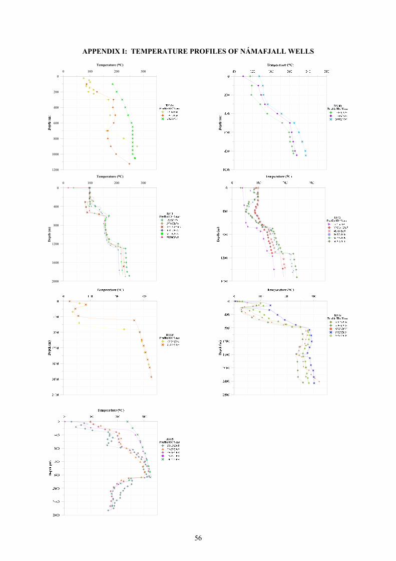
56
APPENDIX I: TEMPERATURE PROFILES OF NÁMAFJALL WELLS
1200
1000
800
600
400
200
0
0 100 200 300
Temperature (oC)
2000
1600
1200
800
400
0
Dep
th(m
)
0 100 200 300
Temperature (oC)
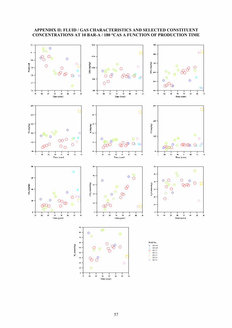
57
APPENDIX II: FLUID / GAS CHARACTERISTICS AND SELECTED CONSTITUENT CONCENTRATIONS AT 10 BAR-A / 180 °CAS A FUNCTION OF PRODUCTION TIME
SiO
2(m
g/k
g)
Na
(mg/
kg)
Cl(
mg/
kg)
CO
2(m
mol
/kg)
75 80 85 90 95 00 05 10
Time (year)
0
10
20
30
40
50
60
70
80
90
H2
(mm
ol/k
g)