Embed Size (px)
Citation preview

Arc Flash Hazards on Photovoltaic Arrays
End of Semester Report, Spring 2013
David Smith
Prepared to Partially Fulfill the Requirements of ECE 402
Department of Electrical and Computer Engineering
Colorado State University
Fort Collins, Colorado 80523
Project Advisor: Dr. George Collins
Industry Sponsor: Dohn Simms, Praxis Corporation
Approved by: Dr George Collins

Abstract
For the second semester of my senior project, I chose to focus on the subject of arc flash
hazards in utility‐scale photovoltaic arrays. As an electrician, this subject combines my
interests in electrical worker safety and the continued rapid pace of the development of
alternative methods of generating electricity. This subject is of great practical interest to
Facility and Project Managers who are responsible for the safety of their workers but must
also balance this concern with the need to maintain a reliable system with minimal
downtime.
An arc flash is a sustained arcing current that propagates through the conductive plasma
created by the breakdown of a gaseous dielectric medium, typically air. Given the right
conditions, the current will continue to flow unabated until interrupted by an upstream
over‐current protective device. Such arcs release enormous energy, resulting in high
temperatures, sound levels, pressures and the ejection of high‐speed molten debris.
Much of the existing research into predicting arc flash energies is specific to alternating
current. The empirically derived equations in the Institute of Electrical and Electronics
Engineer’s ‘Guide to Performing Arc‐Flash Hazard Calculations’ (IEEE Standard 1584) applies
only to arcs in AC systems. Currently, no consensus standard exists for calculating arc
energies in DC systems. However, the 2012 edition of the National Fire Protection
Association’s ‘Standard for Electrical Safety in the Workplace’ (NFPA 70E) references two
papers that offer theoretical and semi‐empirical methods for estimating DC arc energy.
This report presents the results obtained in performing a comparative analysis of these two
methods for predicting DC arc energy as applied to an existing 30 MW photovoltaic array. It
should be noted that no high‐power empirical testing was performed as part of this project;
hence all values provided here are purely theoretical and specific to the San Luis Solar Farm
in Alamosa, Colorado.
In general, fault currents on the array are quite low compared to AC systems, and hence arc
energies are correspondingly low in the short time scale. However, clearing faults on the
array with traditional time‐overcurrent devices is problematic, and under certain conditions
it may be possible for faults to persist for much longer than the 2 second maximum often
assumed in arc flash studies. At 2 seconds, the calculation methods utilized returned values
as high as 17 and 8 calories/cm2, respectively, high enough to present a significant hazard to
electrical workers.

ContentsAbstract ......................................................................................................................................................... 2
Figures ........................................................................................................................................................... 3
Introduction .................................................................................................................................................. 4
System Short Circuit Current ........................................................................................................................ 4
Fault‐Clearing Devices ................................................................................................................................... 6
Arcing Current and Fault Clearing Time ........................................................................................................ 9
Arc Length ................................................................................................................................................... 11
Incident Energy ........................................................................................................................................... 13
Enclosure Multiplying Factor ...................................................................................................................... 14
Comparison of Values between Methods .................................................................................................. 15
Conclusions ................................................................................................................................................. 17
Future Work ................................................................................................................................................ 18
References .................................................................................................................................................. 19
Acknowledgements ..................................................................................................................................... 19
Appendix A: Abbreviations ......................................................................................................................... 20
Appendix B: Project Costs .......................................................................................................................... 20
Appendix C: Additional Materials ............................................................................................................... 21
Figures
Figure 1: Sunpower Module Electrical Data .................................................................................................. 5
Figure 2: Ground Fault .................................................................................................................................. 7
Figure 3: Ground Fault with Pre‐existing Fault ............................................................................................. 8
Figure 4: Positive to Negative Fault .............................................................................................................. 8
Figure 5: Arc Equivalent Circuit ..................................................................................................................... 9
Figure 6: System for Implementing Ammerman Equation (Zg = Arc Gap = 90mm) .................................... 10
Figure 7: Time‐Current Curve of Inverter Fuse ............................................................................................ 10
Figure 8: Arc Power as Function Arc Current .............................................................................................. 11
Figure 9: Arc Resistance as a Function of Arc Gap ...................................................................................... 12
Figure 10: Combiner Box Arc Gap ............................................................................................................... 12
Figure 11: 'k' as a Function of Enclosure Size .............................................................................................. 14
Figure 12: 'a' as a Function of Enclosure Size .............................................................................................. 15
Figure 13: IE Values, MPP and Ammerman ................................................................................................ 16
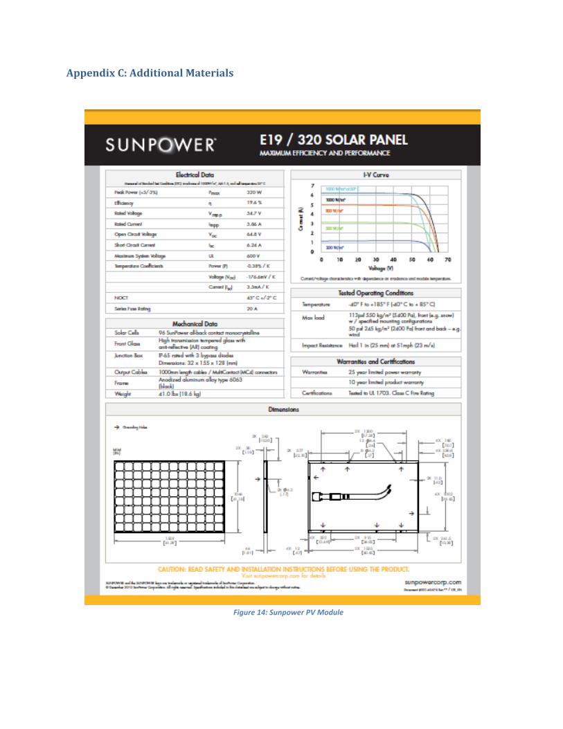
Figure 14: Sunpower PV Module ................................................................................................................. 21
Figure 15: Inverter Fuse Curve .................................................................................................................... 22
Figure 16: String Fuse Curve ........................................................................................................................ 23

IntroductionWith the growth in recent years of utility‐scale solar photovoltaic farms commonly arranged
in arrays that produce between 600 and 1000 volts DC, it is becoming increasingly important
to explore whether dangerous arcs can develop on the DC bus, and if so, to evaluate
methods for predicting the energies workers might be exposed to. Free‐burning arcs of the
sort that can be inadvertently struck by an electrical worker are very complex, difficult to
accurately model and are evaluated from a “black box” perspective in this paper. The two
methods used to predict arc energy on the San Luis Solar Farm, both cited in the 2012
version of the NFPA 70E, are:
Maximum Power Method, developed by Dan Doan in his 2007 paper “Arc Flash
Calculations for Exposures to DC Systems” [1]
Semi‐empirical method, developed by Dr. Ravel Ammerman, et al, in their 2009
paper “DC Arc Models and Incident Energy Calculations” [2]
The maximum power method is essentially a DC version of Lee’s method [3], and relies on
the premise that the maximum power transferred to a resistive load—the arc resistance in
this case—occurs when the load resistance is equal to that of the source. Theoretically, this
method will provide worst case values, but it is a relatively simple approach that computes
arc energy as a function of the system voltage and available bolted fault current only.
The Ammerman method is based on a review of historical laboratory data from several
disparate studies spanning more than a century. Where these data sets could be reasonably
compared, good agreement was generally found in the Volt‐Amp characteristic of the DC
arc. An equation describing the non‐linear nature of arc resistance was developed from one
of the most extensive sets of data, and is the equation used throughout this paper. Unlike
the maximum power method, this relationship incorporates differences in arc length and
offers a way to predict the arc resistance and hence the arcing current.
SystemShortCircuitCurrentAs in any arc flash study, the first step is building an accurate model of the system and
computing the available short circuit current at all worker accessible nodes that would
require an arc flash hazard label. The San Luis facility is composed of over 100,000 320 Watt
modules arranged in series strings of thirteen, with between 222 and 225 strings feeding 38
inverters. The inverters are galvanically isolated power electronic devices that should not be
capable of supplying power from the AC grid to the DC bus. Hence we have treated the farm
as 38 essentially identical, isolated arrays. The only difference between these individual
arrays is the number of strings and some small differences in conductor length due to the
placement of the inverters relative to their associated strings. We have focused on 1‐INV‐A
(222 strings) and 19‐INV‐B (225 strings) in order to capture the full range of currents
available on the farm.
The Volt‐Amp curve of a photovoltaic module is non‐linear, and the cell will act as either a
constant current or a constant voltage source depending on region of operation, which is
determined by the load resistance. The maximum power that can be provided by the module
occurs at the transition between the two regions and is the point at which the maximum
power point tracking system will attempt to hold the array. Current, and voltage to a much
lesser extent, depends on solar irradiance and temperature. Standard Test Conditions for
measuring a module’s Volt‐Amp characteristic are a solar irradiance of 1000 Watts/m2 and
25⁰ Celsius. The manufacturer data for the 320 Watt Sunpower modules used on the San
Luis farm is shown below:
Figure 1: Sunpower Module Electrical Data
Unfortunately, solar irradiance is not constant, nor is 1000 Watts/m2 a maximum possible
value, so predicting the current that may be flowing in the system at fault inception is
difficult. In the interests of providing a worst‐case value, a high‐irradiance factor of 125% has
been applied to all computed currents in the system. This can be a problematic strategy
when faults are cleared by time‐overcurrent devices, since a higher fault current may
indicate a faster clearing time and hence a lower arc energy. However, as will be discussed
later, faults cleared by time‐overcurrent devices on this farm will likely be of such long
duration that this will not be a meaningful issue.
Bus voltage is determined by the 13 series modules and, assuming the farm is operating
anywhere near the maximum power point, will stay within a relatively narrow band over a
large range of solar irradiance values. Further, low impedance faults in the array will sag the
voltage, and push the operating point back into the constant current region of the Volt‐Amp
curve. Hence, the values for calculations throughout this paper are based on a bus voltage of
711 V (54.7 Volts*13 modules) and 125% of the short circuit current rating of n modules,
depending on the location. Accounting for conductor resistance, the range of values are
1,571 A at Combiner Box 1‐A1‐1, and 1,734 A and Inverter 19‐INV‐B.
Fault‐ClearingDevicesUnlike faults in other types of systems, particularly AC systems with rotating machines where
fault currents are typically several times the nominal operating current, the available fault
current in a photovoltaic array is limited by the amount of solar radiation that is currently
falling on the modules, and this current will vary very little over a wide range of operating
voltages. Hence the fault currents in the system are essentially re‐directed operating
currents, and traditional time‐overcurrent devices may not clear faults quickly or at all.
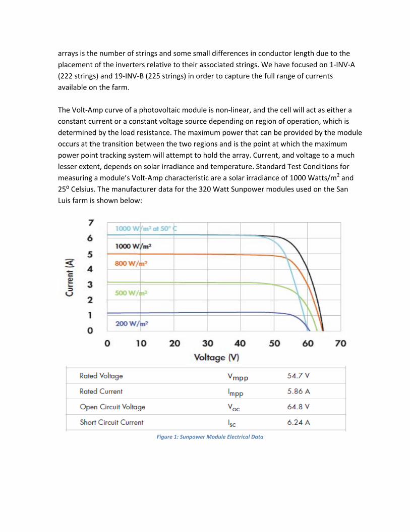
On the San Luis farm, there are 10 A fuses in the combiner boxes at the end of each 13
module string and 315 A fuses in the inverters at the end of each feeder from the combiner
boxes. The positive pole of the array is grounded through calibrated resistors as part of the
Ground Fault Protective Device (GFPD). A rise in voltage across these resistors, indicating
increased current flow above a small, constant “leakage” current, will trigger the device,
rapidly opening the array’s connection to ground and to the AC grid. The GFPD should
operate for any relatively low‐impedance fault, as long as the fault current is in excess of the
normal leakage current that flows from the positive pole to ground through the GFPD
resistors. Figure 1 below shows the fault current path in the event of a ground fault:
Figure 2: Ground Fault
In this case, the current will flow from the grounded positive pole to the fault point, which
has been forced to a lower potential, opening the GFPD and the DC contactor in the inverter,
leaving no available path and clearing the fault.
However, in his 2012 paper, “The Ground‐Fault Protection Blind Spot: A safety Concern For
Larger Photovoltaic Systems In The United States” [4], Bill Brooks identified a scenario under
which the GFPD might fail to clear a ground fault, and postulated that this was the cause of
two recent fires at large solar arrays. In this scenario, a high‐impedance ground fault could
develop and persist indefinitely if the current was below the leakage current previously
referred to. Now if a low impedance ground fault were to occur, the GFPD would trip as
before, but the pre‐existing high‐impedance path could develop into a path capable of
supplying much of the available current to second fault point. This scenario is shown in
Figure 2 below, where points A and B indicate different possible locations for the pre‐
existing fault. If at point A, the second fault would likely trip the string fuse and be cleared
relatively quickly. At point B, the clearing device would be the inverter fuse which requires
more current than is available in the system to operate quickly:
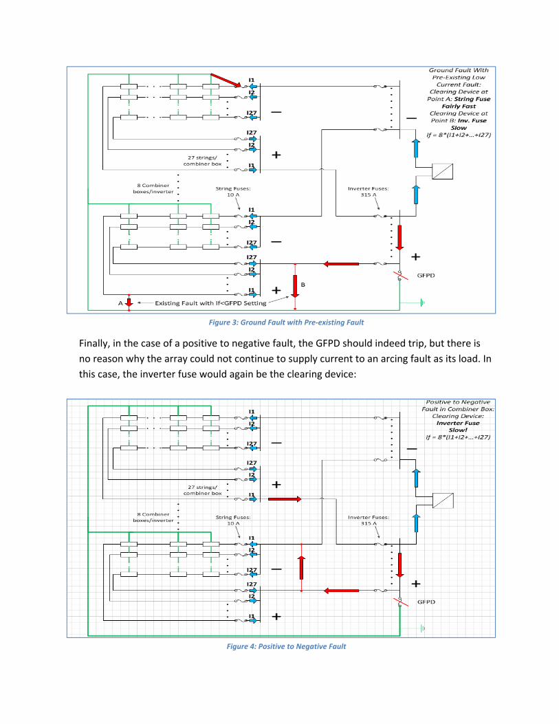
Figure 3: Ground Fault with Pre‐existing Fault
Finally, in the case of a positive to negative fault, the GFPD should indeed trip, but there is
no reason why the array could not continue to supply current to an arcing fault as its load. In
this case, the inverter fuse would again be the clearing device:
Figure 4: Positive to Negative Fault
ArcingCurrentandFaultClearingTimeAs previously mentioned, the lack of significant current rise during a fault on a photovoltaic
array presents a problem when the fault must be cleared by a time‐overcurrent device. Even
assuming a bolted fault at the inverter terminals with the highest available current, 1734 A,
the time‐current characteristics of the inverter fuse are such that it would require
approximately 4.5 seconds to open. Since the total energy in the arc increases linearly with
time, this very long fault clearing time can lead to dangerously high incident energies.
Accurately predicting the potential energy a worker might be exposed to requires the ability
to estimate the arc impedance, and hence the arcing current.
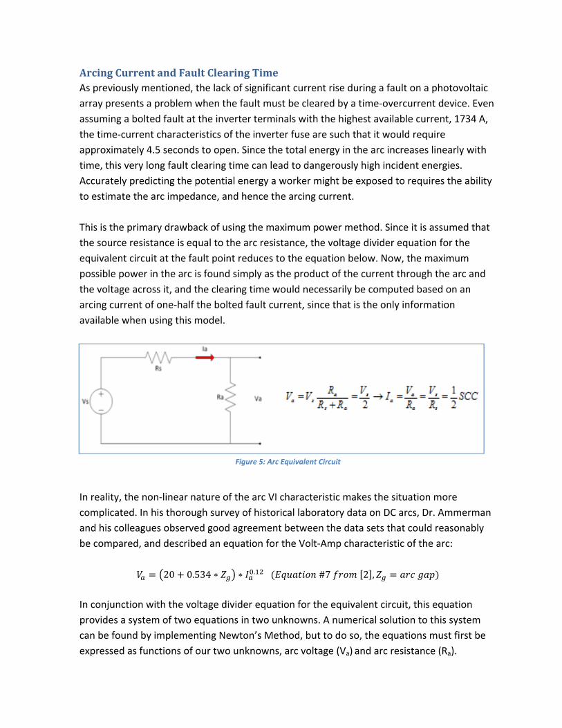
This is the primary drawback of using the maximum power method. Since it is assumed that
the source resistance is equal to the arc resistance, the voltage divider equation for the
equivalent circuit at the fault point reduces to the equation below. Now, the maximum
possible power in the arc is found simply as the product of the current through the arc and
the voltage across it, and the clearing time would necessarily be computed based on an
arcing current of one‐half the bolted fault current, since that is the only information
available when using this model.
Figure 5: Arc Equivalent Circuit
In reality, the non‐linear nature of the arc VI characteristic makes the situation more
complicated. In his thorough survey of historical laboratory data on DC arcs, Dr. Ammerman
and his colleagues observed good agreement between the data sets that could reasonably
be compared, and described an equation for the Volt‐Amp characteristic of the arc:
20 0.534 ∗ ∗ . #7 2 ,
In conjunction with the voltage divider equation for the equivalent circuit, this equation
provides a system of two equations in two unknowns. A numerical solution to this system
can be found by implementing Newton’s Method, but to do so, the equations must first be
expressed as functions of our two unknowns, arc voltage (Va) and arc resistance (Ra).
Depending on an appropriate guess for the initial values of the unknowns, the solution will
converge rapidly:
Figure 6: System for Implementing Ammerman Equation (Zg = Arc Gap = 90mm)
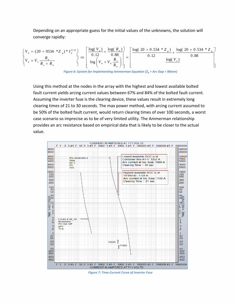
Using this method at the nodes in the array with the highest and lowest available bolted
fault current yields arcing current values between 67% and 84% of the bolted fault current.
Assuming the inverter fuse is the clearing device, these values result in extremely long
clearing times of 21 to 30 seconds. The max power method, with arcing current assumed to
be 50% of the bolted fault current, would return clearing times of over 100 seconds, a worst
case scenario so imprecise as to be of very limited utility. The Ammerman relationship
provides an arc resistance based on empirical data that is likely to be closer to the actual
value.
Figure 7: Time‐Current Curve of Inverter Fuse
)log(88.0
*534.020log(
12.0
)*534.020log(
log
88.0
)log(
12.0
)log(*)*053420( 12.0
s
gg
a
saa
aa
as
asa
aga
V
ZZ
R
RVV
RV
RR
RVV
IZV

ArcLengthAnother advantage provided by Dr. Ammerman’s work over the max power method is the
ability predict arc characteristics based on the estimated arc length. As Dr. Ammerman
observed, the voltage across an arc is almost independent of the arcing current above a
certain ‘transition current’, and is proportional to the length of the arc. The arc resistance
will increase with length, and hence power is greater in a longer arc. Plots of arc power as a
function of arcing current are shown below for different arc gaps inside the maximum power
envelope as given by a fixed system voltage and resistance:
Figure 8: Arc Power as Function Arc Current
The same information presented in terms of arc resistance shows how the power in the arc
increases significantly with arc length:

Figure 9: Arc Resistance as a Function of Arc Gap
While the actual arc length is not exactly the length of the gap between the electrodes,
particularly for horizontal arcs, this gap can at least approximate the length of the arc and
should be accurately measured given the relatively large changes in power for different arc
lengths. In the combiner boxes on the San Luis Farm, the gap between the positive and
negative terminals is approximately 90 mm, much larger than the 32 mm that is often
assumed for AC equipment in the same voltage class:
Figure 10: Combiner Box Arc Gap
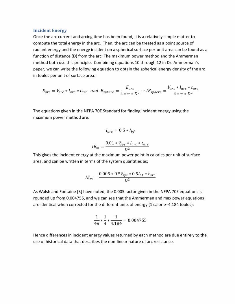
IncidentEnergyOnce the arc current and arcing time has been found, it is a relatively simple matter to
compute the total energy in the arc. Then, the arc can be treated as a point source of
radiant energy and the energy incident on a spherical surface per‐unit area can be found as a
function of distance (D) from the arc. The maximum power method and the Ammerman
method both use this principle. Combining equations 10 through 12 in Dr. Ammerman’s
paper, we can write the following equation to obtain the spherical energy density of the arc
in Joules per unit of surface area:
∗ ∗ 4 ∗ ∗
→∗ ∗4 ∗ ∗
The equations given in the NFPA 70E Standard for finding incident energy using the
maximum power method are:
0.5 ∗
0.01 ∗ ∗ ∗
This gives the incident energy at the maximum power point in calories per unit of surface
area, and can be written in terms of the system quantities as:
0.005 ∗ 0.5 ∗ 0.5 ∗
As Walsh and Fontaine [3] have noted, the 0.005 factor given in the NFPA 70E equations is
rounded up from 0.004755, and we can see that the Ammerman and max power equations
are identical when corrected for the different units of energy (1 calorie=4.184 Joules):
14
∗14∗
14.184
0.004755
Hence differences in incident energy values returned by each method are due entirely to the
use of historical data that describes the non‐linear nature of arc resistance.
EnclosureMultiplyingFactorThe equations above will yield an estimate for the energy radiated equally in all directions by
an arc in open air. However, we are most interested arcs that might develop in the combiner
boxes and at the inverter terminals, as these are the system nodes where technicians are
most likely to be required to perform work on energized parts. Testing performed by the
IEEE 1584 working group [6] on AC arcs demonstrated that the energy of an arc in an
enclosure will reflect off the interior surfaces, resulting in higher incident energy at the
opening of the enclosure. As written in the NFPA 70E Standard [7], the max power method
simply suggests the open air incident energy be increased by a factor of three for arcs in
enclosures of any size. However, using the 1584 data for the three enclosure sizes that were
tested, Robert Wilkins developed an equation for estimating the arc energy in an enclosure
[5]:
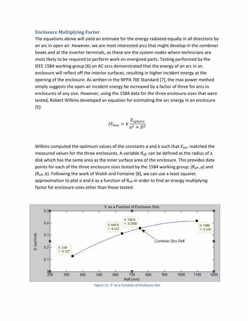
Wilkins computed the optimum values of the constants a and k such that Ebox matched the
measured values for the three enclosures. A variable Reff can be defined as the radius of a
disk which has the same area as the inner surface area of the enclosure. This provides data
points for each of the three enclosure sizes tested by the 1584 working group: (Reff ,a) and
(Reff ,k). Following the work of Walsh and Fontaine [8], we can use a least squares
approximation to plot a and k as a function of Reff in order to find an energy multiplying
factor for enclosure sizes other than those tested:
Figure 11: 'k' as a Function of Enclosure Size
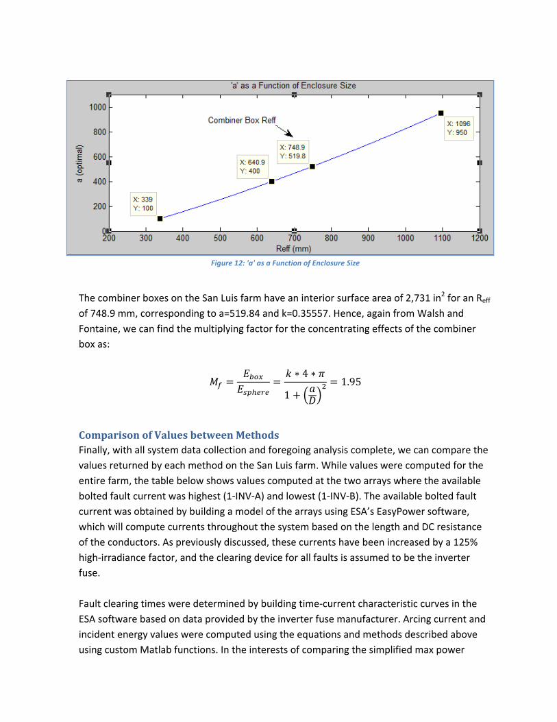
Figure 12: 'a' as a Function of Enclosure Size
The combiner boxes on the San Luis farm have an interior surface area of 2,731 in2 for an Reff
of 748.9 mm, corresponding to a=519.84 and k=0.35557. Hence, again from Walsh and
Fontaine, we can find the multiplying factor for the concentrating effects of the combiner
box as:
∗ 4 ∗
11.95
ComparisonofValuesbetweenMethodsFinally, with all system data collection and foregoing analysis complete, we can compare the
values returned by each method on the San Luis farm. While values were computed for the
entire farm, the table below shows values computed at the two arrays where the available
bolted fault current was highest (1‐INV‐A) and lowest (1‐INV‐B). The available bolted fault
current was obtained by building a model of the arrays using ESA’s EasyPower software,
which will compute currents throughout the system based on the length and DC resistance
of the conductors. As previously discussed, these currents have been increased by a 125%
high‐irradiance factor, and the clearing device for all faults is assumed to be the inverter
fuse.
Fault clearing times were determined by building time‐current characteristic curves in the
ESA software based on data provided by the inverter fuse manufacturer. Arcing current and
incident energy values were computed using the equations and methods described above
using custom Matlab functions. In the interests of comparing the simplified max power
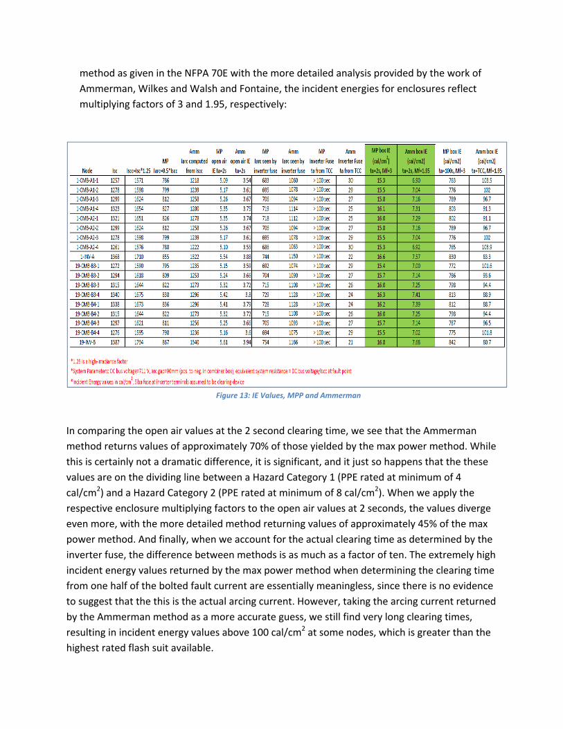
method as given in the NFPA 70E with the more detailed analysis provided by the work of
Ammerman, Wilkes and Walsh and Fontaine, the incident energies for enclosures reflect
multiplying factors of 3 and 1.95, respectively:
Figure 13: IE Values, MPP and Ammerman
In comparing the open air values at the 2 second clearing time, we see that the Ammerman
method returns values of approximately 70% of those yielded by the max power method. While
this is certainly not a dramatic difference, it is significant, and it just so happens that the these
values are on the dividing line between a Hazard Category 1 (PPE rated at minimum of 4
cal/cm2) and a Hazard Category 2 (PPE rated at minimum of 8 cal/cm2). When we apply the
respective enclosure multiplying factors to the open air values at 2 seconds, the values diverge
even more, with the more detailed method returning values of approximately 45% of the max
power method. And finally, when we account for the actual clearing time as determined by the
inverter fuse, the difference between methods is as much as a factor of ten. The extremely high
incident energy values returned by the max power method when determining the clearing time
from one half of the bolted fault current are essentially meaningless, since there is no evidence
to suggest that the this is the actual arcing current. However, taking the arcing current returned
by the Ammerman method as a more accurate guess, we still find very long clearing times,
resulting in incident energy values above 100 cal/cm2 at some nodes, which is greater than the
highest rated flash suit available.
Section B.1.2 in Annex B of the IEEE 1584 [5] Standard allows for the use of 2 seconds as the
maximum clearing time, based entirely on the idea that a person exposed to an arc flash will
move away quickly if it is “physically possible,” and this principle is generally accepted
throughout the industry. However, as noted in the 1584 Standard, “a person who is in a bucket
truck or a person who has crawled into equipment will require more time to get away.” There
are at least two significant problems with this principle: first, how do we reasonably quantify
how much “more time” is enough time for workers who are working in a non‐optimal position?
Second, it is not uncommon for victims of arc flashes and blasts to be knocked unconscious and
hence be incapable of moving away from the arc. Further, if system conditions are found to be
such that clearing times are likely to be in excess of 2 seconds, this is a serious design deficiency
that could result in catastrophic damage to equipment as well as posing a hazard to workers.
ConclusionsPotential incident energy on the DC bus of the San Luis Solar Farm at worker accessible nodes
as computed by the two methods is high enough to merit concern, and in some cases may be
above the level that can realistically be mitigated by PPE . As expected, the semi‐empirical
Ammerman method returns lower incident energy values in all cases.
It is important to note again that the methods used to obtain the values presented in this paper
are suggested by the NFPA 70E Standard, and that there is currently no codified methodology
based on empirical test results for computing DC arc energies, such as the IEEE 1584 standard
for AC systems. Further, wide deployment of utility‐scale photovoltaic arrays is a relatively
recent development, so there is a dearth of recorded incidents on solar farms from which to
draw conclusions about the likelihood and potential severity of arc flashes and blasts on the DC
bus. As such, good engineering judgment and a conservative approach should be taken in
evaluating DC arc flash hazards until comprehensive testing can be conducted.
That said, requiring workers to don overly burdensome protective gear can lower productivity,
limit movement and vision and even potentially increase the chances of initiating a fault. Given
the consistency of the historical data presented by Dr. Ammerman and his co‐authors, it is
reasonable to use the method presented in that paper as a less conservative and likely more
accurate approach. Further, the ability to compute arcing current and hence arcing time is a
major improvement over the maximum power method.
Available fault currents on the San Luis farm are relatively low compared to those found in AC
systems since they are essentially redirected line currents, so incident energy values for short‐
duration faults will be correspondingly low. While the Ground Fault Protective Device should
detect most low‐impedance faults on the array and operate very quickly, it is only capable of
disconnecting the array from the inverter and the positive pole of the array from earth ground.
Under certain conditions, the GFPD may not interrupt the flow of fault current and the inverter
fuse would have to be the clearing device. In these cases, the low fault current could lead to
long clearing times and correspondingly high incident energy. Deciding to use the “2 second
rule” or any clearing time other than that given by the time‐current characteristics of the
inverter fuse is problematic and should be done only after careful consideration of the tasks
that may be performed on energized equipment.
FutureWorkThere is a lot of uncertainty inherent in any Arc Flash Study, even those conducted on AC
systems using the empirical formulas given by the IEEE 1584 Standard, but that uncertainty is
greater here. There is a need for comprehensive testing in a high‐power lab under a variety of
test setups. In particular, attempts should be made to create free‐burning arcs when the DC
voltage is relatively high (600V‐1000V) and the available fault current is relatively low in order
duplicate the conditions found on a typical photovoltaic array. Further, it is generally assumed
that DC arcs will be less susceptible to self‐extinction than AC arcs since there are no zero‐
crossings; investigation into whether long‐duration arcs can be sustained at these relatively low
fault currents would be valuable.
While there is a rapidly growing selection of fuses designed specifically for photovoltaic
applications, and reducing clearing times with judicious fuse changes may be a possibility, it
seems likely that low fault currents relative to nominal currents will continue to make
traditional time‐overcurrent devices problematic on solar farms. Investigation into novel
system protections schemes beyond time‐overcurrent and ground fault devices could be
fruitful. Differential relaying and fiberoptic light detectors are methods that have been used in
other applications and might be applied here. However, it is interruption, rather than detection,
that is the main problem. What is needed is an interrupting device in series with the inverter
fuses that can be opened based on a trip signal from whatever overcurrent detection scheme is
used.

References[1] DC Arc Models and Incident Energy Calculations, Ammerman, Gammon, Sen, Nelson, 2009
[2] Arc Flash Calculations for Exposures to DC Systems, Daniel R. Doan, 2007
[3] The other Electrical Hazard: Electric Arc Blast Burns, Ralph H. Lee, 1982
[4] The Ground‐Fault Protection Blind Spot: A Safety Concern for Larger Photovoltaic Systems In
the United States, Bill Brooks, 2012
[5] Simple Improved Equations for Arc Flash Hazard Analysis, Robert Wilkins, 2004
[6] Guide for Performing Arc Flash Hazard Calculations, IEEE 1584‐2002, 2002
[7] Standard for Electrical Safety in the Workplace, NFPA 70E, 2012
[8] DC Arc Flash Calculations‐Arc‐in‐Open‐Air & Arc‐in‐a‐Box‐Using a Simplified Approach
(Multiplication Factor Method), Michael Fontaine and Peter Walsh, 2012
AcknowledgementsI would like to thank Mr. Simms and Dr. Collins for their guidance throughout the semester and
for their patience as I slowly learned the background material necessary for understanding this
subject. I would also like to thank John Kolak for his constant optimism and tireless
encouragement when it was most needed.

AppendixA:AbbreviationsIEEE: Institute of Electrical and Electronics Engineers
NFPA: National Fire Protections Association
SCC: Short Circuit Current
IE: Incident Energy
TCC: Time‐Current Curve
XFMR: Power Transformer
AppendixB:ProjectCostsTravel:
– 2 trips to Alamosa for data collection. 255 miles each way
• At $0.555/mi (gsa.gov)
• 255*4*$0.555=$566.10
Research paper costs:
– $10 each from IEEE explore
• 6 total for $60
E‐days poster:
– $20
Total expenses: $646.10
AppendixC:AdditionalMaterials
Figure 14: Sunpower PV Module
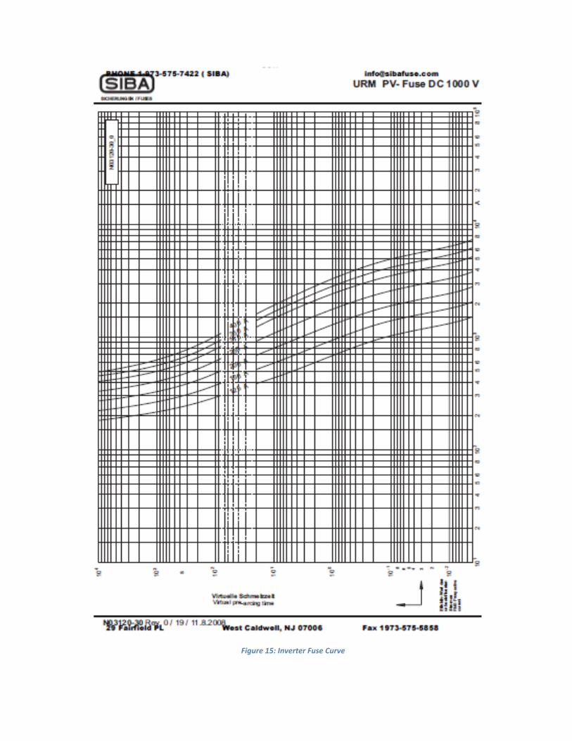
Figure 15: Inverter Fuse Curve

Figure 16: String Fuse Curve