Embed Size (px)
Citation preview
Informed Search
Introduction to informed search
The A* search algorithm
Designing good admissible heuristics
(AIMA Chapter 3.5.1, 3.5.2, 3.6)
Outline – Informed Search
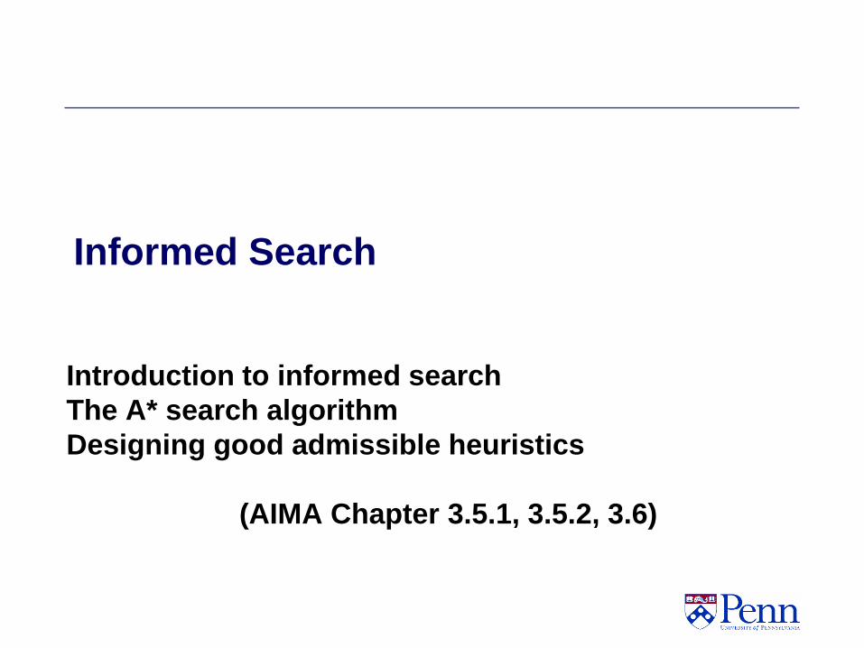
PART I - Today
Informed = use problem-specific knowledge
Best-first search and its variants
A* - Optimal Search using Knowledge
Proof of Optimality of A*
A* for maneuvering AI agents in games
Heuristic functions?
How to invent them
PART II Local search and optimization
• Hill climbing, local beam search, genetic algorithms,…
Local search in continuous spaces
Online search agents
2CIS 391 - Intro to AI
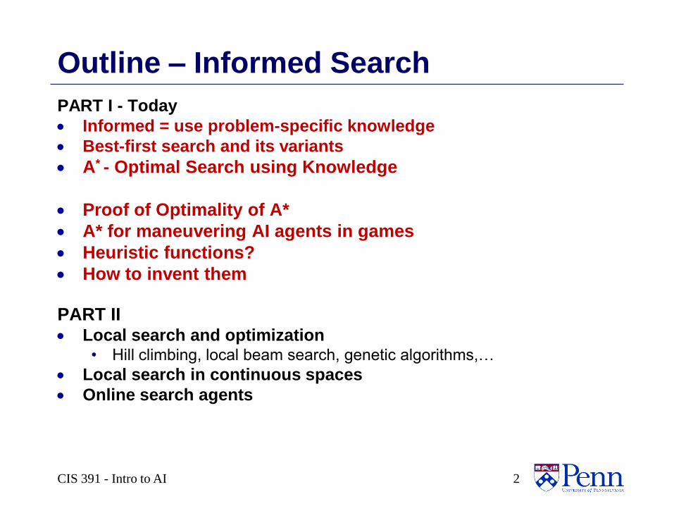
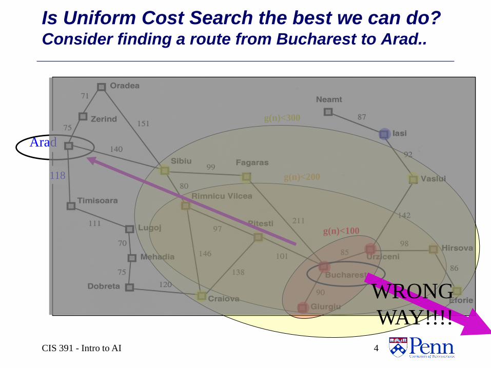
Is Uniform Cost Search the best we can do? Consider finding a route from Bucharest to Arad..
Arad
118
3CIS 391 - Intro to AI
g(n)<100
g(n)<300
g(n)<200
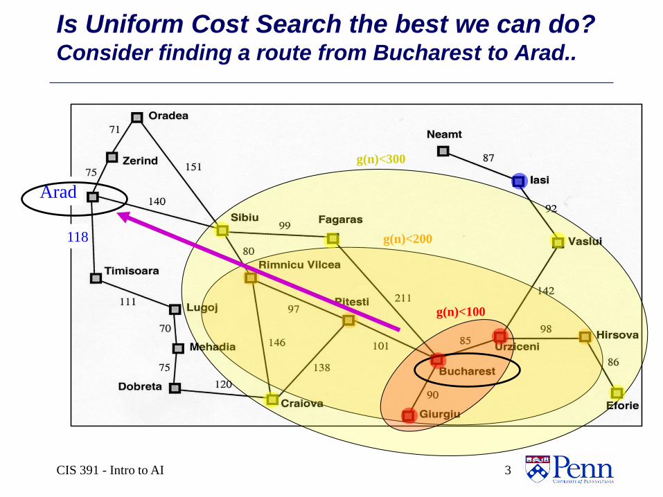
Is Uniform Cost Search the best we can do? Consider finding a route from Bucharest to Arad..
Arad
118
4
g(n)<300
CIS 391 - Intro to AI
g(n)<100
g(n)<200
WRONG
WAY!!!!
A Better Idea…
Node expansion based on an estimate which
includes distance to the goal
General approach of informed search:
• Best-first search: node selected for expansion based
on an evaluation function f(n)
—f(n) includes estimate of distance to goal (new
idea!)
Implementation: Sort frontier queue by this new f(n).
• Special cases: greedy search, A* search
5CIS 391 - Intro to AI
Arad
118
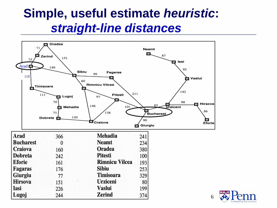
Simple, useful estimate heuristic:
straight-line distances
6CIS 391 - Intro to AI
Heuristic (estimate) functions
Heureka! ---Archimedes
[dictionary]“A rule of thumb, simplification, or educated guess that reduces or limits the search for solutions in domains that are difficult and poorly understood.”
Heuristic knowledge is useful, but not necessarily correct.
Heuristic algorithms use heuristic knowledge to solve a problem.
A heuristic function h(n) takes a state n and returns an estimate of the distance from n to the goal.
(graphic: http://hyperbolegames.com/2014/10/20/eureka-moments/)
CIS 391 - Intro to AI 7
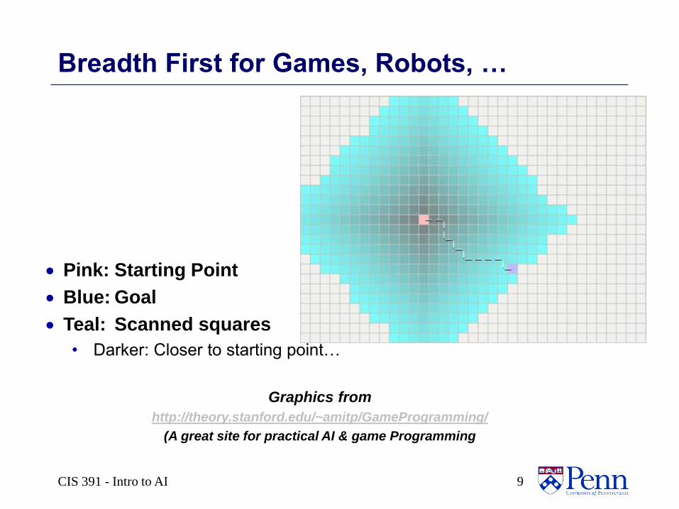
Breadth First for Games, Robots, …
Pink: Starting Point
Blue: Goal
Teal: Scanned squares
• Darker: Closer to starting point…
Graphics from
http://theory.stanford.edu/~amitp/GameProgramming/
(A great site for practical AI & game Programming
9CIS 391 - Intro to AI
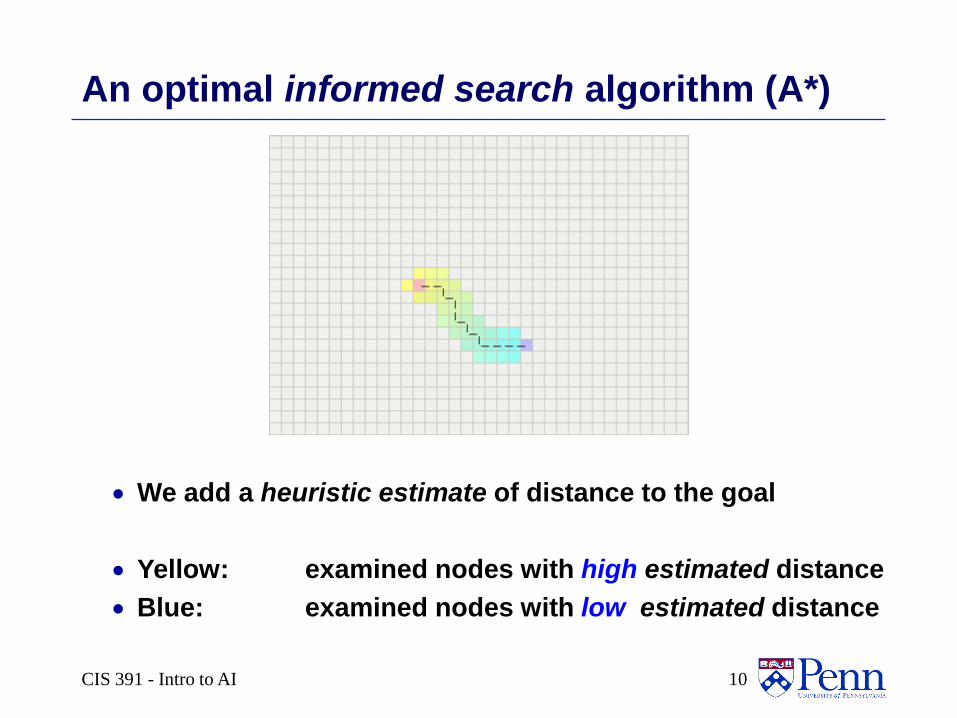
An optimal informed search algorithm (A*)
We add a heuristic estimate of distance to the goal
Yellow: examined nodes with high estimated distance
Blue: examined nodes with low estimated distance
10CIS 391 - Intro to AI
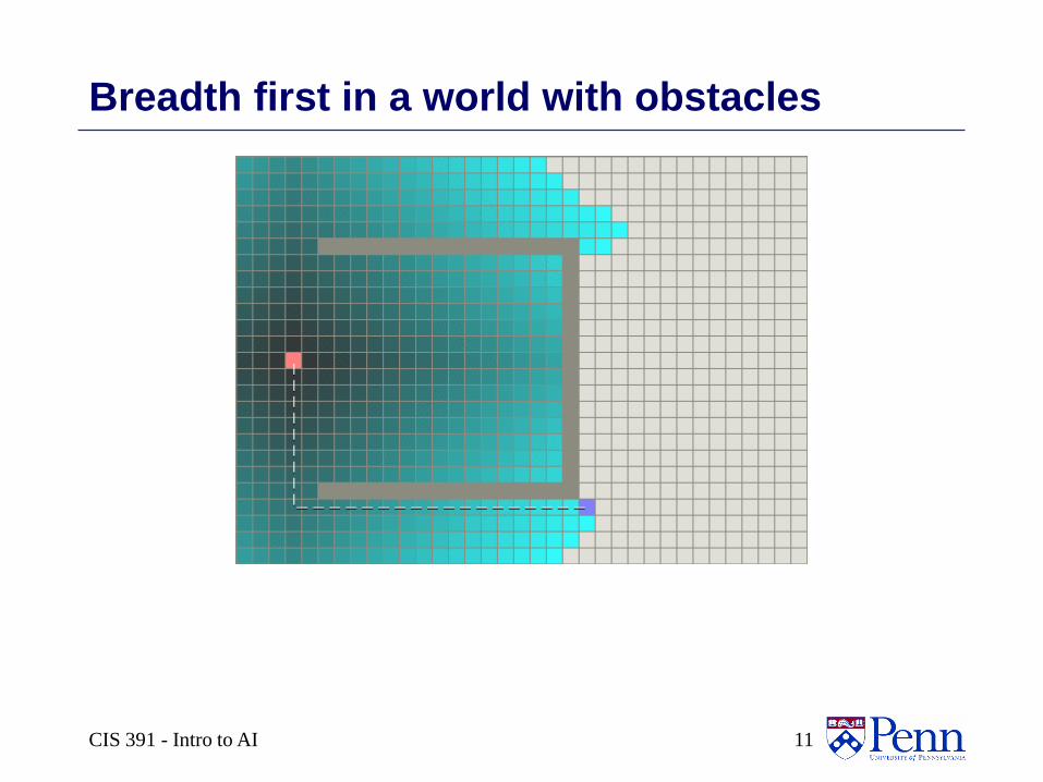
Breadth first in a world with obstacles
11CIS 391 - Intro to AI
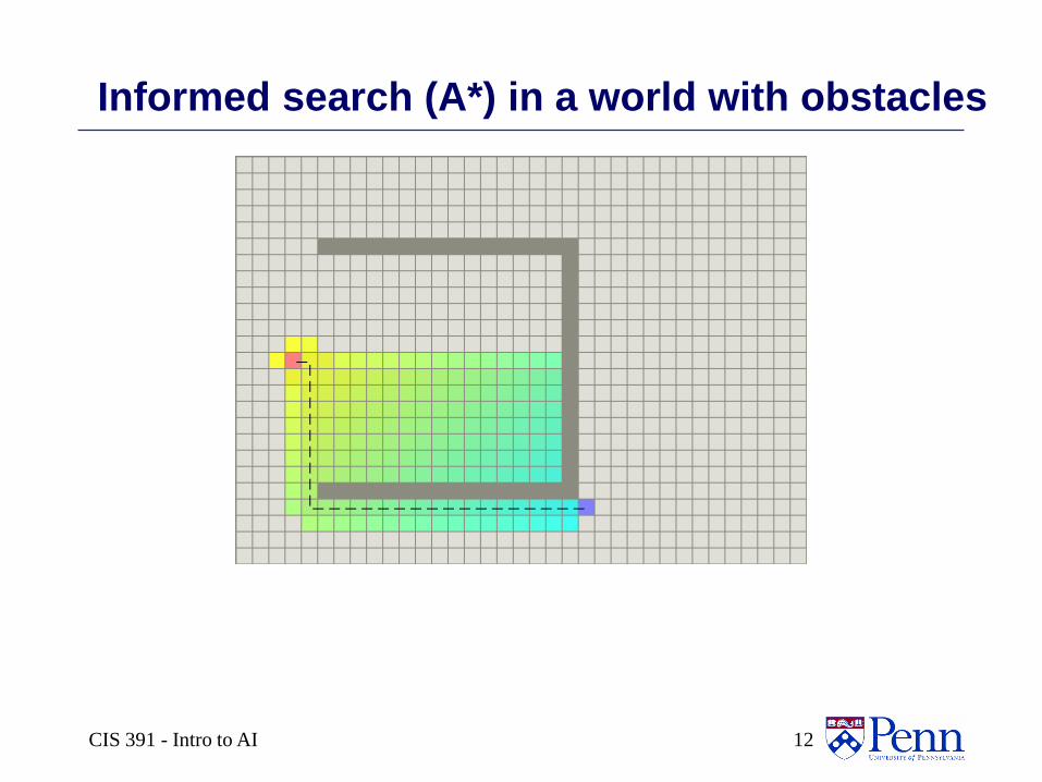
Informed search (A*) in a world with obstacles
12CIS 391 - Intro to AI
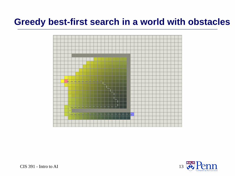
Greedy best-first search in a world with obstacles
CIS 391 - Intro to AI 13
Review: Best-first search
Basic idea:
select node for expansion with minimal
evaluation function f(n)
• where f(n) is some function that includes estimate heuristic
h(n) of the remaining distance to goal
Implement using priority queue
Exactly UCS with f(n) replacing g(n)
14CIS 391 - Intro to AI
Greedy best-first search: f(n) = h(n)
Expands the node that is estimated to be closest
to goal
Completely ignores g(n): the cost to get to n
Here, h(n) = hSLD(n) = straight-line distance from `
to Bucharest
15CIS 391 - Intro to AI
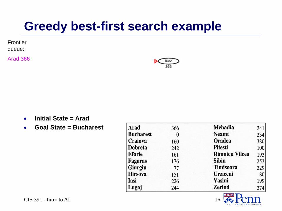
Greedy best-first search example
Initial State = Arad
Goal State = Bucharest
Frontier
queue:
Arad 366
16CIS 391 - Intro to AI
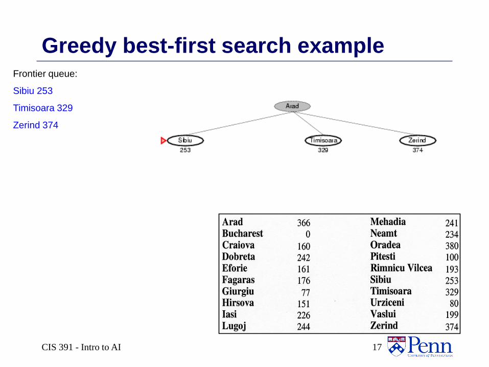
Greedy best-first search exampleFrontier queue:
Sibiu 253
Timisoara 329
Zerind 374
17CIS 391 - Intro to AI
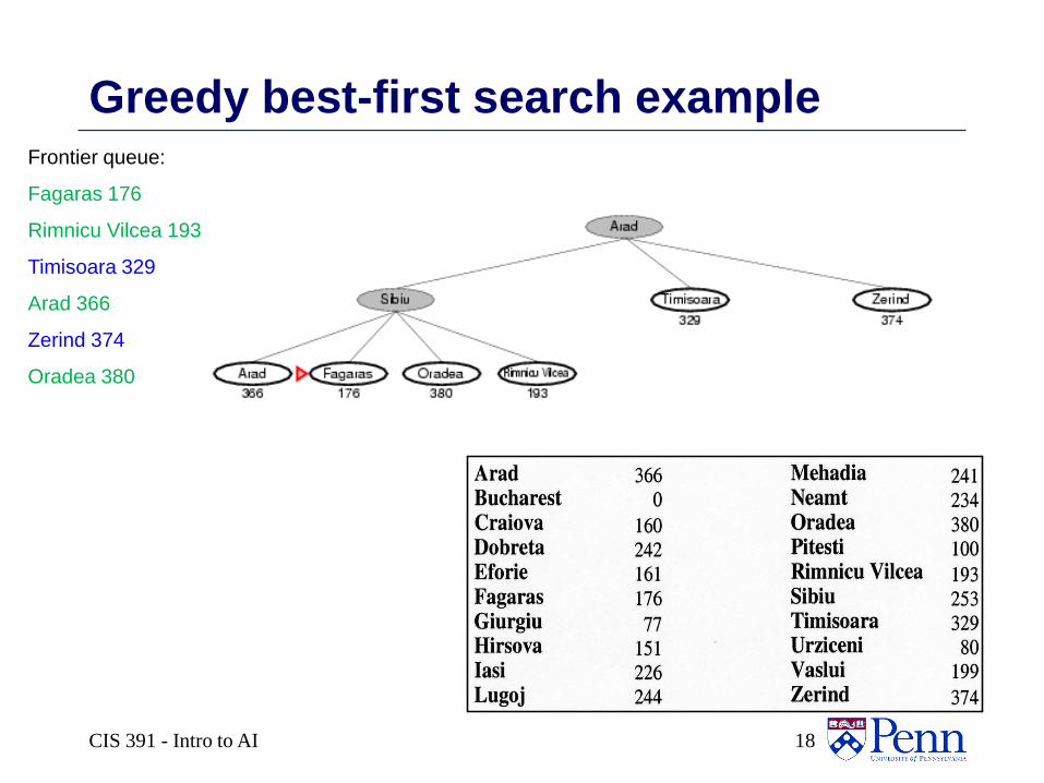
Greedy best-first search exampleFrontier queue:
Fagaras 176
Rimnicu Vilcea 193
Timisoara 329
Arad 366
Zerind 374
Oradea 380
18CIS 391 - Intro to AI
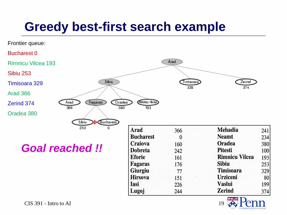
Greedy best-first search example
Goal reached !!
Frontier queue:
Bucharest 0
Rimnicu Vilcea 193
Sibiu 253
Timisoara 329
Arad 366
Zerind 374
Oradea 380
19CIS 391 - Intro to AI
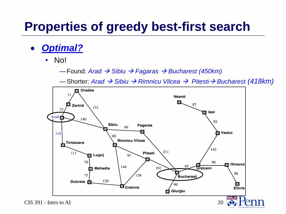
Properties of greedy best-first search
Optimal?
• No!
—Found: Arad Sibiu Fagaras Bucharest (450km)
—Shorter: Arad Sibiu Rimnicu Vilcea Pitesti Bucharest (418km)
Arad
118
20CIS 391 - Intro to AI
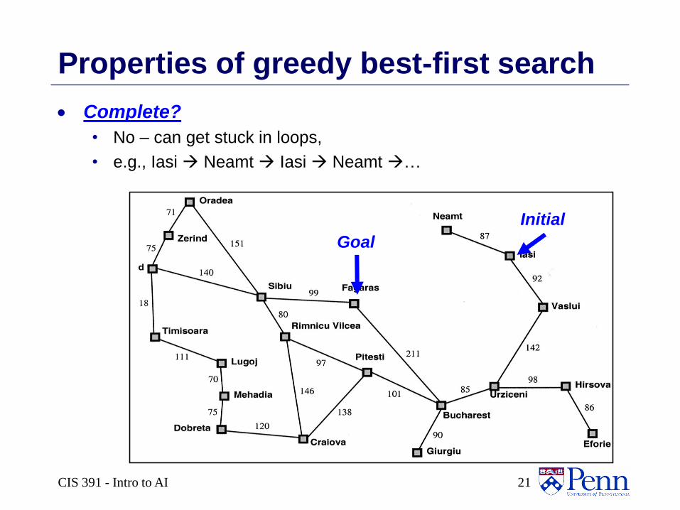
Properties of greedy best-first search
Complete?
• No – can get stuck in loops,
• e.g., Iasi Neamt Iasi Neamt …
Goal
Initial
21CIS 391 - Intro to AI
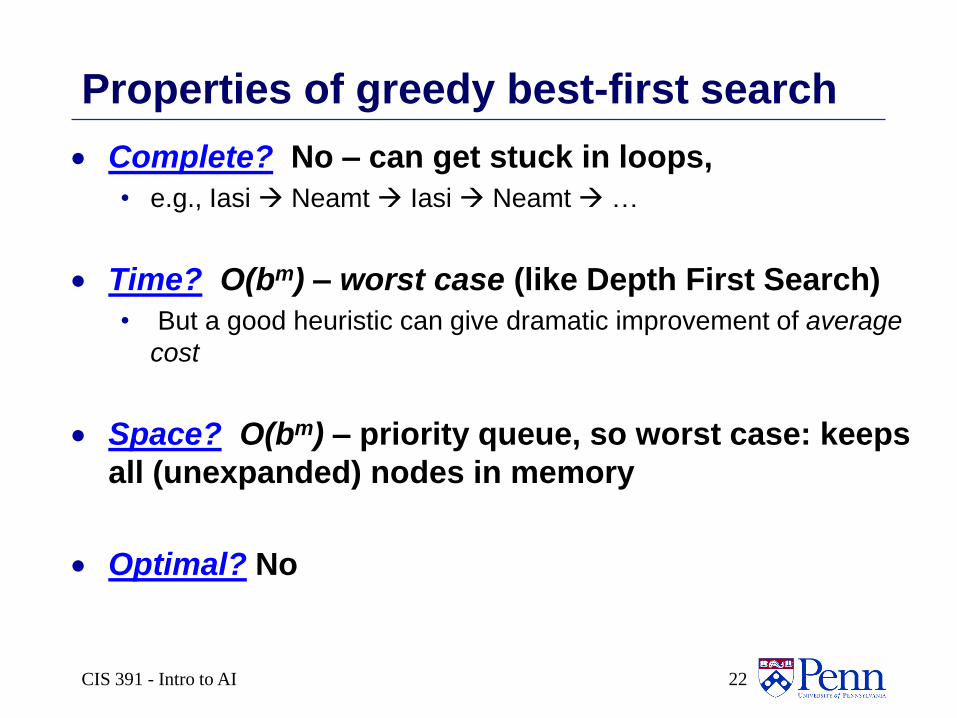
Properties of greedy best-first search
Complete? No – can get stuck in loops,
• e.g., Iasi Neamt Iasi Neamt …
Time? O(bm) – worst case (like Depth First Search)
• But a good heuristic can give dramatic improvement of average
cost
Space? O(bm) – priority queue, so worst case: keeps
all (unexpanded) nodes in memory
Optimal? No
22CIS 391 - Intro to AI
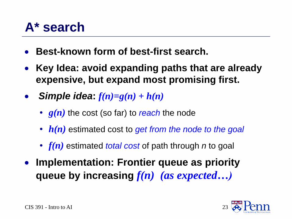
A* search
Best-known form of best-first search.
Key Idea: avoid expanding paths that are already
expensive, but expand most promising first.
Simple idea: f(n)=g(n) + h(n)
• g(n) the cost (so far) to reach the node
• h(n) estimated cost to get from the node to the goal
• f(n) estimated total cost of path through n to goal
Implementation: Frontier queue as priority
queue by increasing f(n) (as expected…)
23CIS 391 - Intro to AI
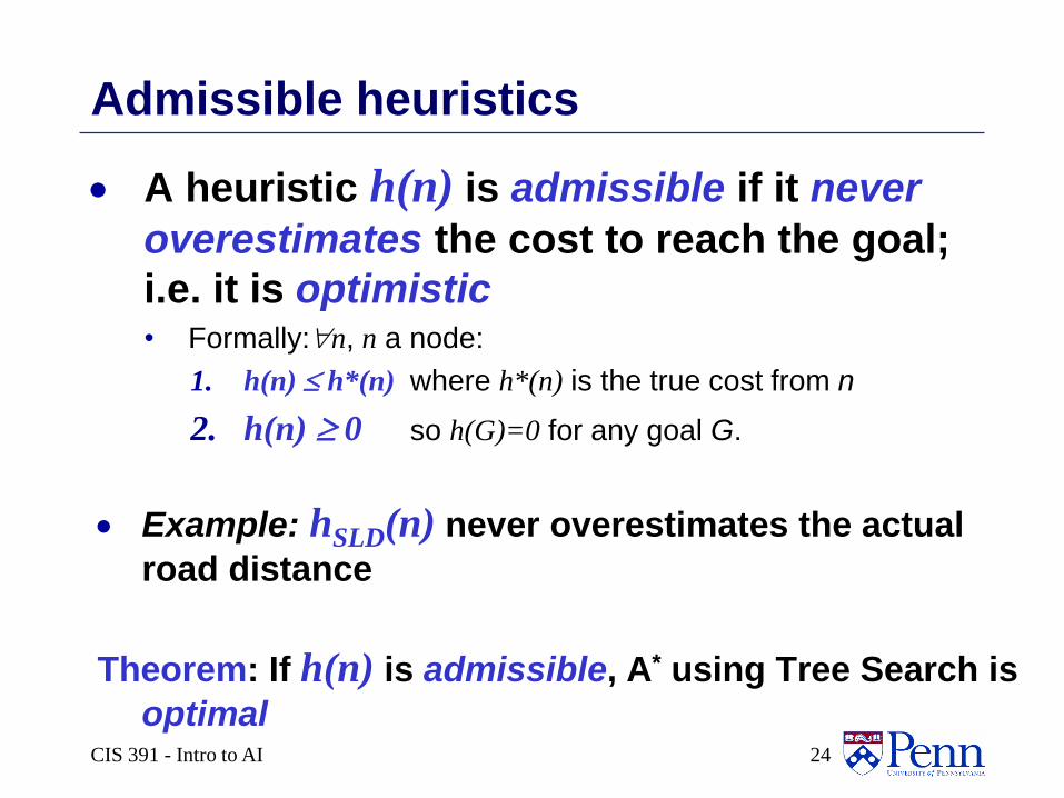
Admissible heuristics
A heuristic h(n) is admissible if it never
overestimates the cost to reach the goal;
i.e. it is optimistic• Formally:n, n a node:
1. h(n) h*(n) where h*(n) is the true cost from n
2. h(n) 0 so h(G)=0 for any goal G.
Example: hSLD(n) never overestimates the actual
road distance
Theorem: If h(n) is admissible, A* using Tree Search is
optimal24CIS 391 - Intro to AI
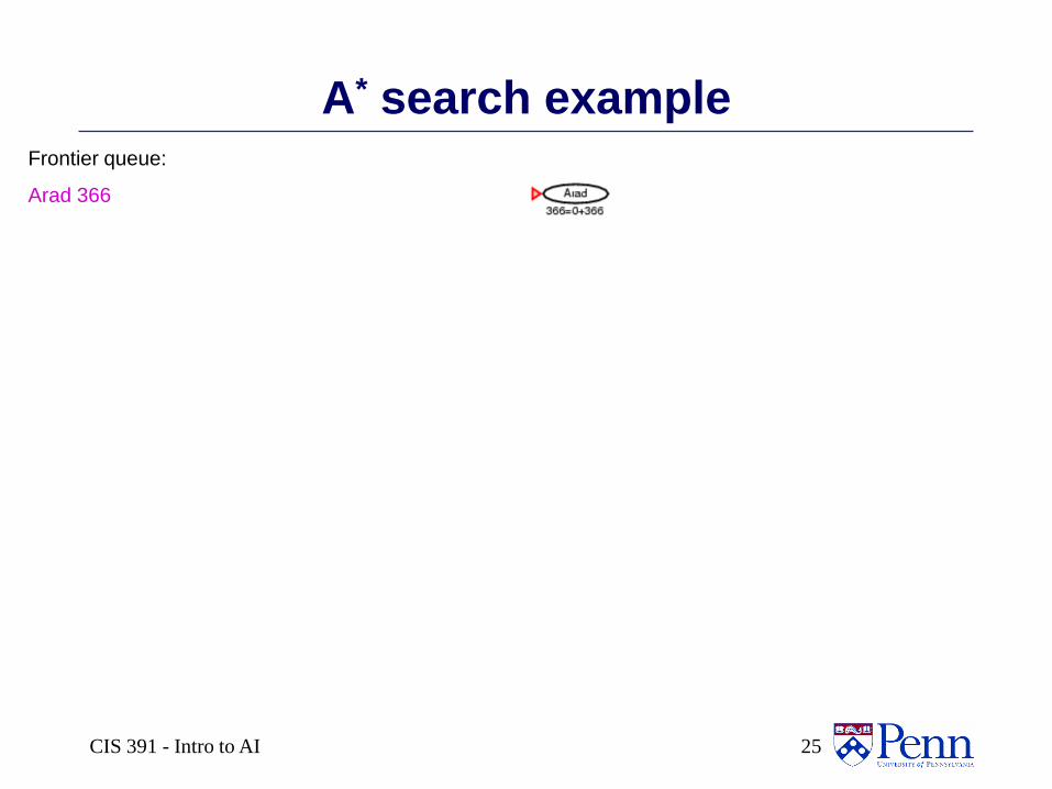
A* search exampleFrontier queue:
Arad 366
25CIS 391 - Intro to AI
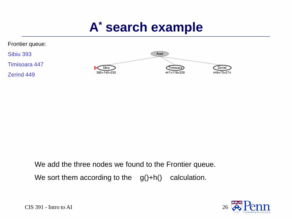
A* search exampleFrontier queue:
Sibiu 393
Timisoara 447
Zerind 449
We add the three nodes we found to the Frontier queue.
We sort them according to the g()+h() calculation.
26CIS 391 - Intro to AI
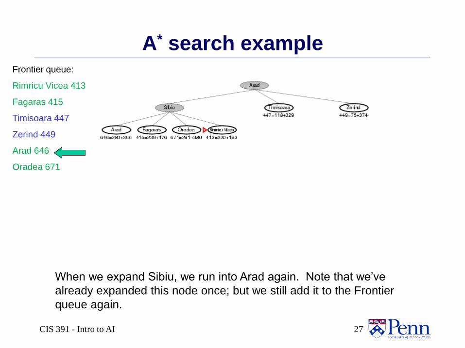
A* search exampleFrontier queue:
Rimricu Vicea 413
Fagaras 415
Timisoara 447
Zerind 449
Arad 646
Oradea 671
When we expand Sibiu, we run into Arad again. Note that we’ve
already expanded this node once; but we still add it to the Frontier
queue again.
27CIS 391 - Intro to AI
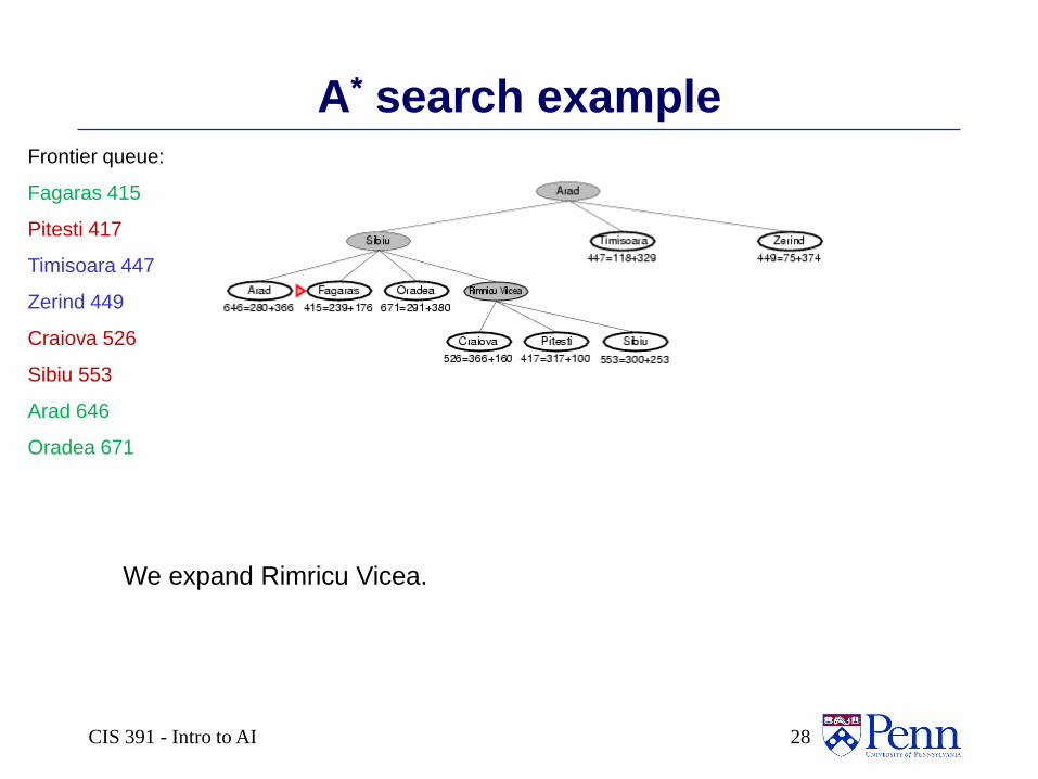
A* search exampleFrontier queue:
Fagaras 415
Pitesti 417
Timisoara 447
Zerind 449
Craiova 526
Sibiu 553
Arad 646
Oradea 671
We expand Rimricu Vicea.
28CIS 391 - Intro to AI
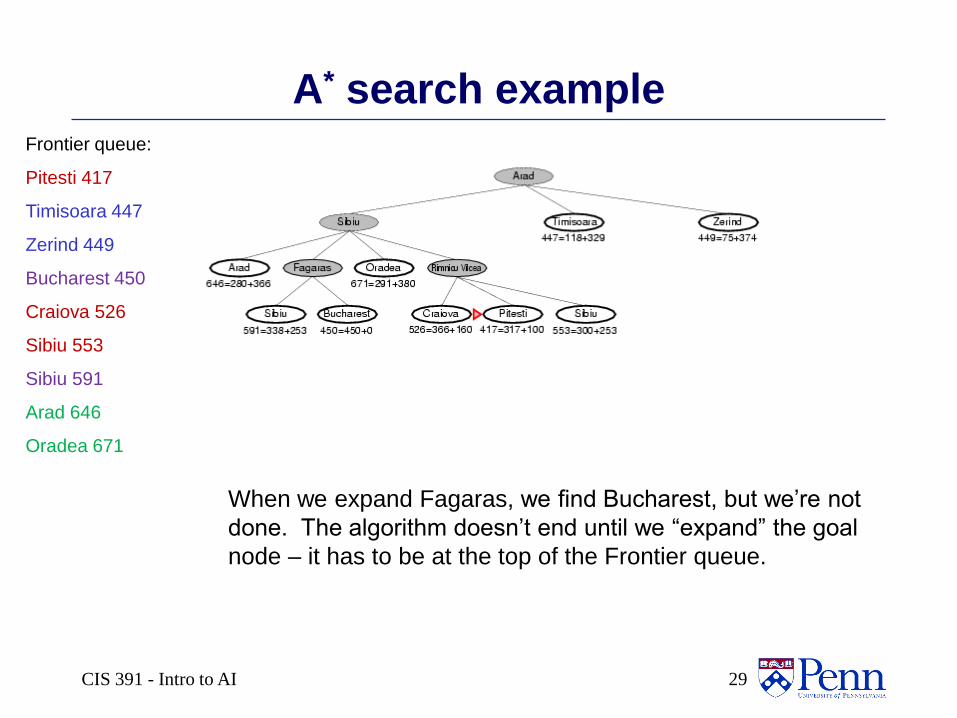
A* search exampleFrontier queue:
Pitesti 417
Timisoara 447
Zerind 449
Bucharest 450
Craiova 526
Sibiu 553
Sibiu 591
Arad 646
Oradea 671
When we expand Fagaras, we find Bucharest, but we’re not
done. The algorithm doesn’t end until we “expand” the goal
node – it has to be at the top of the Frontier queue.
29CIS 391 - Intro to AI
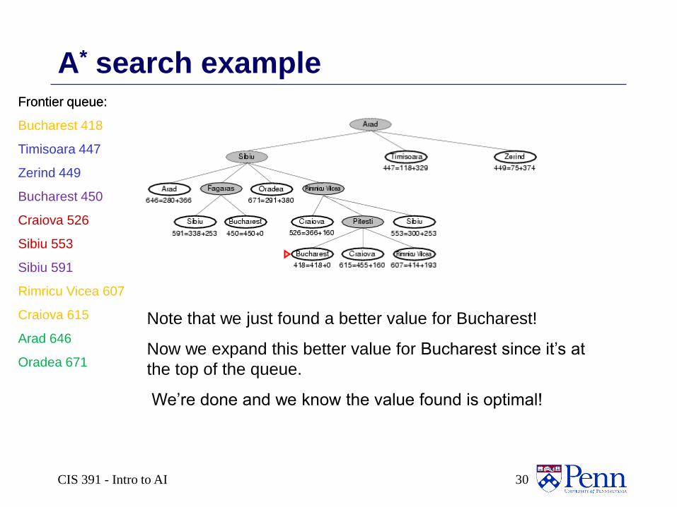
A* search exampleFrontier queue:
Note that we just found a better value for Bucharest!
Now we expand this better value for Bucharest since it’s at
the top of the queue.
We’re done and we know the value found is optimal!
Frontier queue:
Bucharest 418
Timisoara 447
Zerind 449
Bucharest 450
Craiova 526
Sibiu 553
Sibiu 591
Rimricu Vicea 607
Craiova 615
Arad 646
Oradea 671
30CIS 391 - Intro to AI
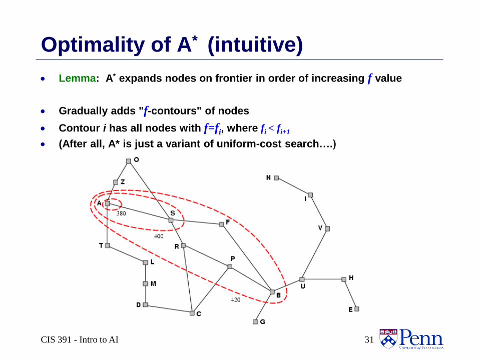
Optimality of A* (intuitive)
Lemma: A* expands nodes on frontier in order of increasing f value
Gradually adds "f-contours" of nodes
Contour i has all nodes with f=fi, where fi < fi+1
(After all, A* is just a variant of uniform-cost search….)
31CIS 391 - Intro to AI
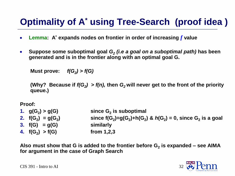
Lemma: A* expands nodes on frontier in order of increasing f value
Suppose some suboptimal goal G2 (i.e a goal on a suboptimal path) has been generated and is in the frontier along with an optimal goal G.
Must prove: f(G2) > f(G)
(Why? Because if f(G2) > f(n), then G2 will never get to the front of the priority queue.)
Proof:
1. g(G2) > g(G) since G2 is suboptimal
2. f(G2) = g(G2) since f(G2)=g(G2)+h(G2) & h(G2) = 0, since G2 is a goal
3. f(G) = g(G) similarly
4. f(G2) > f(G) from 1,2,3
Also must show that G is added to the frontier before G2 is expanded – see AIMA for argument in the case of Graph Search
Optimality of A* using Tree-Search (proof idea )
32CIS 391 - Intro to AI
A* search, evaluation
Completeness: YES
• Since bands of increasing f are added
• As long as b is finite
—(guaranteeing that there aren’t infinitely many nodes n with f (n) < f(G) )
33CIS 391 - Intro to AI
A* search, evaluation
Completeness: YES
Time complexity:
• Number of nodes expanded is still exponential in the length of the solution.
34CIS 391 - Intro to AI
A* search, evaluation
Completeness: YES
Time complexity: (exponential with path length)
Space complexity:
• It keeps all generated nodes in memory
• Hence space is the major problem not time
35CIS 391 - Intro to AI
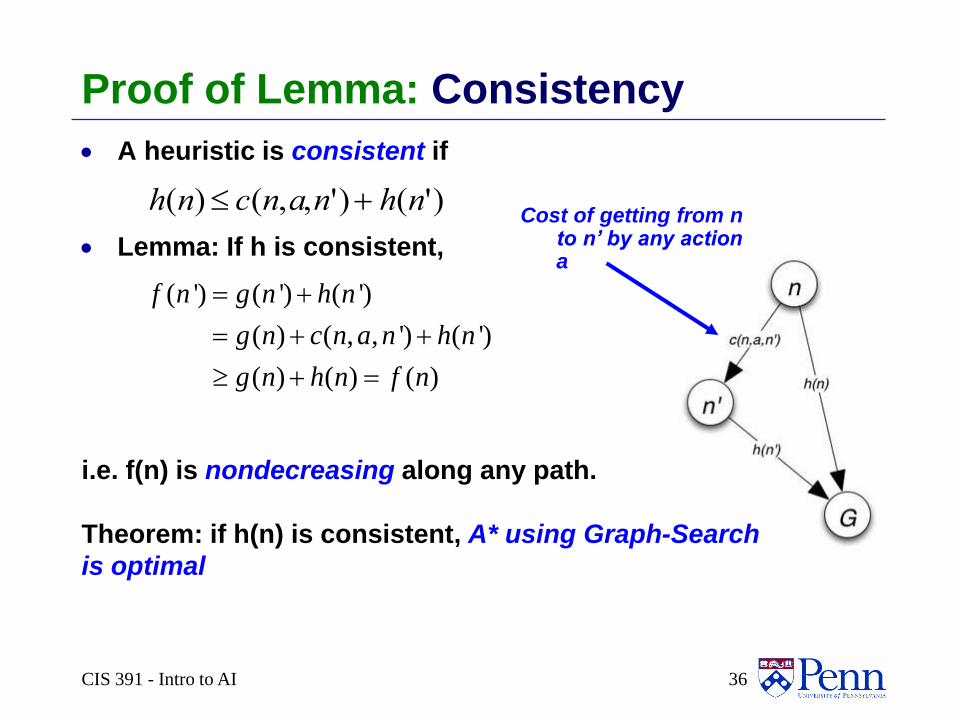
Proof of Lemma: Consistency
A heuristic is consistent if
Lemma: If h is consistent,
i.e. f(n) is nondecreasing along any path.
Theorem: if h(n) is consistent, A* using Graph-Search
is optimal
h(n) c(n,a,n') h(n')
( ') ( ') ( ')
( ) ( , , ') ( ')
( ) ( ) ( )
f n g n h n
g n c n a n h n
g n h n f n
Cost of getting from n to n’ by any action a
36CIS 391 - Intro to AI
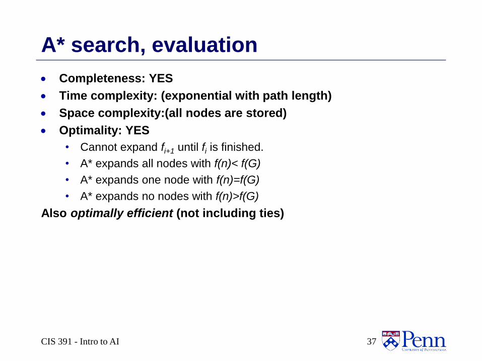
A* search, evaluation
Completeness: YES
Time complexity: (exponential with path length)
Space complexity:(all nodes are stored)
Optimality: YES
• Cannot expand fi+1 until fi is finished.
• A* expands all nodes with f(n)< f(G)
• A* expands one node with f(n)=f(G)
• A* expands no nodes with f(n)>f(G)
Also optimally efficient (not including ties)
37CIS 391 - Intro to AI
Creating Good Heuristic Functions
AIMA 3.6
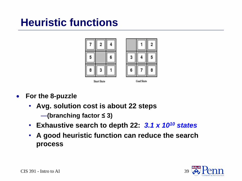
Heuristic functions
For the 8-puzzle
• Avg. solution cost is about 22 steps
—(branching factor ≤ 3)
• Exhaustive search to depth 22: 3.1 x 10¹⁰ states
• A good heuristic function can reduce the search
process
39CIS 391 - Intro to AI
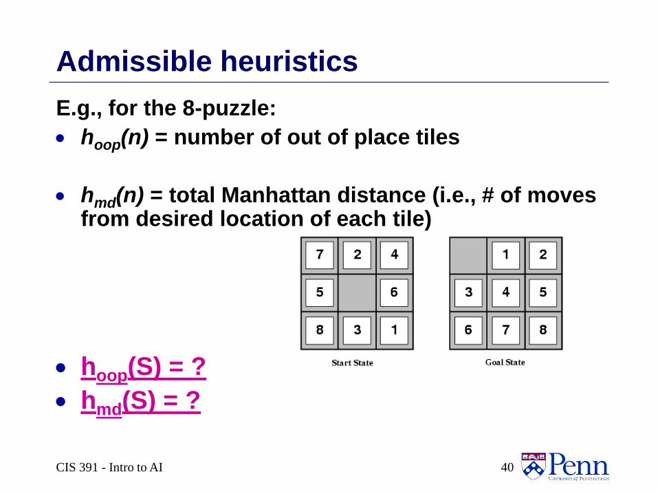
Admissible heuristics
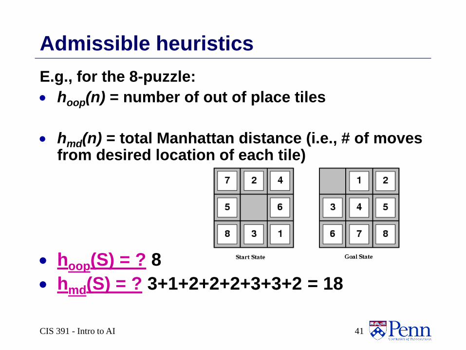
E.g., for the 8-puzzle:
hoop(n) = number of out of place tiles
hmd(n) = total Manhattan distance (i.e., # of moves from desired location of each tile)
hoop(S) = ?
hmd(S) = ?
40CIS 391 - Intro to AI
Admissible heuristics
E.g., for the 8-puzzle:
hoop(n) = number of out of place tiles
hmd(n) = total Manhattan distance (i.e., # of moves from desired location of each tile)
hoop(S) = ? 8
hmd(S) = ? 3+1+2+2+2+3+3+2 = 18
41CIS 391 - Intro to AI
Relaxed problems
A problem with fewer restrictions on the actions than the original is called a relaxed problem
The cost of an optimal solution to a relaxed problem is an admissible heuristic for the original problem
If the rules of the 8-puzzle are relaxed so that a tile can move anywhere, then hoop(n) gives the shortest solution
If the rules are relaxed so that a tile can move to any adjacent square, then hmd(n) gives the shortest solution
42CIS 391 - Intro to AI
Defining Heuristics: h(n)
Cost of an exact solution to a relaxed problem
(fewer restrictions on operator)
Constraints on Full Problem:
A tile can move from square A to square B if A is adjacent to B and
B is blank.
• Constraints on relaxed problems:
—A tile can move from square A to square B if A is adjacent to B.
(hmd)
—A tile can move from square A to square B if B is blank.
—A tile can move from square A to square B. (hoop)
43CIS 391 - Intro to AI
Dominance
If h2(n) ≥ h1(n) for all n (both admissible)
• then h2 dominates h1
So h2 is optimistic, but more accurate than h1
• h2 is therefore better for search
• Notice: hmd dominates hoop
Typical search costs (average number of nodes expanded):• d=12 Iterative Deepening Search = 3,644,035 nodes
A*(hoop) = 227 nodes A*(hmd) = 73 nodes
• d=24 IDS = too many nodesA*(hoop) = 39,135 nodes A*(hmd) = 1,641 nodes
44CIS 391 - Intro to AI
Iterative Deepening A* and beyond
Beyond our scope:
Iterative Deepening A*
Recursive best first search (incorporates A* idea, despite
name)
Memory Bounded A*
Simplified Memory Bounded A* - R&N say the best
algorithm to use in practice, but not described here at all.
• (If interested, follow reference to Russell article on Wikipedia article for
SMA*)
(see 3.5.3 if you’re interested in these topics)
45CIS 391 - Intro to AI