arXiv:astro-ph/0011165 v1 8 Nov 2000 - core.ac.uk · Since the angular momentum of the torus is extracted due to magnetic braking, ... the system evolves ... in the center of a galaxy

arX

iv:a

stro

-ph/

0011

165

v1

8 N

ov 2

000

Resistive Magnetohydrodynamics of Jet Formation and

Magnetically Driven Accretion

Takuhito Kuwabara

Graduate School of Science and Technology, Chiba University, Inage-ku, Chiba 263-8522

E-mail(TK): [email protected]

Kazunari Shibata

Kwasan and Hida Observatories, Kyoto University, Yamashina, Kyoto 607-8471

Takahiro Kudoh

National Astronomical Observatory, Mitaka, Tokyo 181-8588

and

Ryoji Matsumoto

Department of Physics, Faculty of Science, Chiba University, Inage-ku, Chiba 263-8522

(Received 2000 June 16; accepted 2000 August 16)

Abstract

We carried out 2.5-dimensional resistive magnetohydrodynamic simulations to study the

effects of magnetic diffusivity on magnetically driven mass accretion and jet formation. The

initial state is a constant angular-momentum torus threaded by large-scale vertical magnetic

fields. Since the angular momentum of the torus is extracted due to magnetic braking, the torus

medium falls toward the central region. The infalling matter twists the large-scale magnetic

fields and drives bipolar jets. We found that (1) when the normalized magnetic diffusivity,

η ≡ η/(r0VK0), where VK0 is the Keplerian rotation speed at a reference radius r = r0, is small

(η ≤ 10−3), mass accretion and jet formation take place intermittently; (2) when 10−3 ≤ η ≤

10−2, the system evolves toward a quasi-steady state; and (3) when η ≥ 10−2 the accretion/mass

1

outflow rate decreases with η and approaches 0. The results of these simulations indicate that

in the center of a galaxy which has a super-massive (∼ 109 M) black hole, a massive (∼ 108

M) gas torus and magnetic braking provide a mass accretion rate which is sufficient to explain

the activity of AGNs when η ≤ 5 × 10−2.

Key words: accretion, accretion disks — galaxies: active — galaxies: nuclei — galaxies:

jets — MHD

1. Introduction

Magnetically driven outflows from accretion disks are the most promising models of the acceleration

and collimation of jets/winds in AGNs and in star-forming regions. By assuming steady axisymmetric

cold outflow, it has been shown that when the magnetic field lines make angles of less than 60o from the

equatorial plane, a magneto-centrifugally driven outflow of matter emanates from the surface of the disk

(Blandford, Payne 1982; Pudritz, Norman 1983; Lovelace et al. 1986; Shu et al. 1994a,b). Recently, by

including gas pressure, Kudoh and Shibata (1997) obtained a steady solution along a magnetic field line

and showed that when the strength of the poloidal magnetic field, Bp0, is much smaller than the toroidal

component, Bϕ0, the mass outflow rate, Mjet, increases with Bp0 and Mjet approaches a constant value

when Bp0 > Bϕ0.

Several authors have reported the results of axisymmetric two-dimensional magnetohydrodynamic

(MHD) simulations of jet formation by fixing the boundary conditions at the disk surface without includ-

ing the effects of magnetic braking on the disk (e.g., Ustyugova et al. 1995; Meier et al. 1997; Ouyed et

al. 1997). The surface conditions of the accretion disk, however, should be determined self-consistently.

Uchida and Shibata (1985) as well as Shibata and Uchida (1986) carried out nonlinear, two-dimensional

MHD simulations of jet formation from accretion disks by including the effects of a back reaction of jet

formation on disks. They showed that jets/winds are accelerated along the magnetic field lines twisted

by the rotation of the disk. They called this mechanism a “sweeping magnetic twist mechanism”. The

numerical results by Uchida and Shibata (1985) as well as Shibata and Uchida (1986) have been confirmed

by Stone and Norman (1994) by using the ZEUS code. Stone and Norman (1994) have also discussed the

2

relation between magnetic braking and magnetorotational instability (Balbus, Hawley 1991).

The effects of magnetic extraction of angular momentum (magnetic braking) on the disk become

more evident when a geometrically thick disk (or torus) is considered. Matsumoto et al. (1996) carried

out 2D MHD simulations of a torus threaded by poloidal magnetic fields and showed that the surface

layer of the torus accretes faster than the equatorial region, like an avalanche, because magnetic braking

most efficiently extracts angular momentum from that layer. Kudoh, Matsumoto, and Shibata (1998)

confirmed the numerical results by employing a newly developed CIP-MOCCT code which uses the CIP

method (Yabe, Aoki 1991) for hydrodynamic part and the MOCCT scheme (Stone, Norman 1992) to solve

the induction equations and to evaluate the Lorentz force terms. They have proposed that the ejection

mechanism of non-steady jets found in the 2.5-dimensional simulations can be understood using the steady

state theory even when the back reaction of the jet on the disk is included self-consistently. Matsumoto

and Shibata (1997) extended the 2D model to 3D by taking into account the non-axisymmetric effects,

and have shown that the avalanche breaks up into several spiral channels. When the torus is threaded by

large-scale poloidal magnetic field lines, accretion proceeds along these spiral channels. Since the channel

flow bundles the large-scale magnetic field lines, a spiral structure also appears in the jet.

Most of the nonsteady models of magnetohydrodynamic jet formation from an accretion disk have

assumed ideal MHD. Recently, several authors included resistivity to study protostellar jets. Hayashi et

al. (1996) carried out 2D resistive MHD simulations of the interaction of the dipole magnetic field of the

protostar and its surrounding disk and have shown that magnetic reconnection takes place in the current

sheet created inside the expanding magnetic loops. They successfully explained both the acceleration

of optical jets and the X-ray flares in protostars observed by the ASCA satellite (Koyama et al. 1996).

Similar resistive MHD simulations of protostellar jets have been carried out by Miller and Stone (1997),

Grosso et al. (1997), and Goodson et al. (1997, 1999).

Hirose et al. (1997) investigated the interaction of the stellar magnetosphere originated in its

dipole magnetic field and the interstellar magnetic field carried with the infalling gas. They carried out

2D resistive MHD simulations and showed that magnetic reconnection takes place by an interaction of

these magnetic fields. They showed that matter accretes along the reconnected magnetospheric field and

3

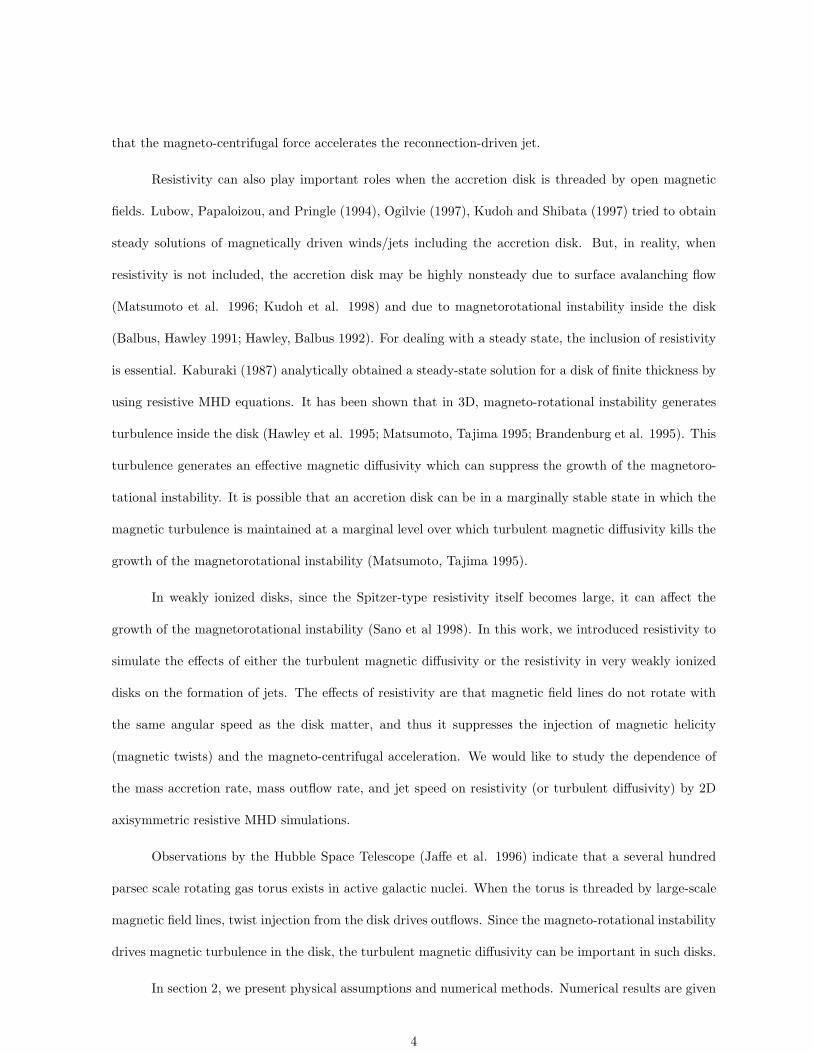
that the magneto-centrifugal force accelerates the reconnection-driven jet.

Resistivity can also play important roles when the accretion disk is threaded by open magnetic

fields. Lubow, Papaloizou, and Pringle (1994), Ogilvie (1997), Kudoh and Shibata (1997) tried to obtain

steady solutions of magnetically driven winds/jets including the accretion disk. But, in reality, when

resistivity is not included, the accretion disk may be highly nonsteady due to surface avalanching flow

(Matsumoto et al. 1996; Kudoh et al. 1998) and due to magnetorotational instability inside the disk

(Balbus, Hawley 1991; Hawley, Balbus 1992). For dealing with a steady state, the inclusion of resistivity

is essential. Kaburaki (1987) analytically obtained a steady-state solution for a disk of finite thickness by

using resistive MHD equations. It has been shown that in 3D, magneto-rotational instability generates

turbulence inside the disk (Hawley et al. 1995; Matsumoto, Tajima 1995; Brandenburg et al. 1995). This

turbulence generates an effective magnetic diffusivity which can suppress the growth of the magnetoro-

tational instability. It is possible that an accretion disk can be in a marginally stable state in which the

magnetic turbulence is maintained at a marginal level over which turbulent magnetic diffusivity kills the

growth of the magnetorotational instability (Matsumoto, Tajima 1995).

In weakly ionized disks, since the Spitzer-type resistivity itself becomes large, it can affect the

growth of the magnetorotational instability (Sano et al 1998). In this work, we introduced resistivity to

simulate the effects of either the turbulent magnetic diffusivity or the resistivity in very weakly ionized

disks on the formation of jets. The effects of resistivity are that magnetic field lines do not rotate with

the same angular speed as the disk matter, and thus it suppresses the injection of magnetic helicity

(magnetic twists) and the magneto-centrifugal acceleration. We would like to study the dependence of

the mass accretion rate, mass outflow rate, and jet speed on resistivity (or turbulent diffusivity) by 2D

axisymmetric resistive MHD simulations.

Observations by the Hubble Space Telescope (Jaffe et al. 1996) indicate that a several hundred

parsec scale rotating gas torus exists in active galactic nuclei. When the torus is threaded by large-scale

magnetic field lines, twist injection from the disk drives outflows. Since the magneto-rotational instability

drives magnetic turbulence in the disk, the turbulent magnetic diffusivity can be important in such disks.

In section 2, we present physical assumptions and numerical methods. Numerical results are given

4

in section 3. Section 4 is devoted to a summary and discussion.

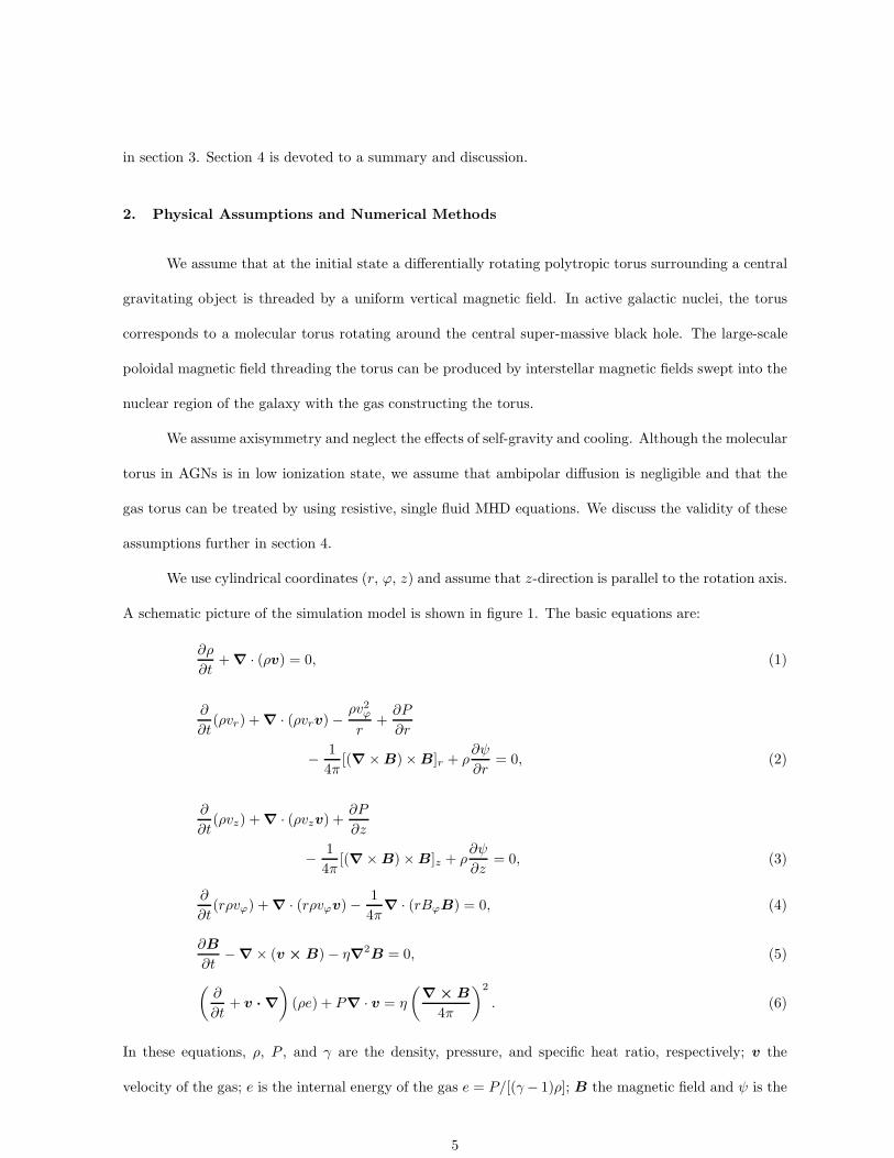
2. Physical Assumptions and Numerical Methods

We assume that at the initial state a differentially rotating polytropic torus surrounding a central

gravitating object is threaded by a uniform vertical magnetic field. In active galactic nuclei, the torus

corresponds to a molecular torus rotating around the central super-massive black hole. The large-scale

poloidal magnetic field threading the torus can be produced by interstellar magnetic fields swept into the

nuclear region of the galaxy with the gas constructing the torus.

We assume axisymmetry and neglect the effects of self-gravity and cooling. Although the molecular

torus in AGNs is in low ionization state, we assume that ambipolar diffusion is negligible and that the

gas torus can be treated by using resistive, single fluid MHD equations. We discuss the validity of these

assumptions further in section 4.

We use cylindrical coordinates (r, ϕ, z) and assume that z-direction is parallel to the rotation axis.

A schematic picture of the simulation model is shown in figure 1. The basic equations are:

∂ρ

∂t+ ∇ · (ρv) = 0, (1)

∂

∂t(ρvr) + ∇ · (ρvrv) −

ρv2ϕ

r+∂P

∂r

− 1

4π[(∇ × B) × B]r + ρ

∂ψ

∂r= 0, (2)

∂

∂t(ρvz) + ∇ · (ρvzv) +

∂P

∂z

− 1

4π[(∇ × B) × B]z + ρ

∂ψ

∂z= 0, (3)

∂

∂t(rρvϕ) + ∇ · (rρvϕv) − 1

4π∇ · (rBϕB) = 0, (4)

∂B

∂t− ∇ × (v × B) − η∇2

B = 0, (5)

(

∂

∂t+ v · ∇

)

(ρe) + P∇ · v = η

(

∇ × B

4π

)2

. (6)

In these equations, ρ, P , and γ are the density, pressure, and specific heat ratio, respectively; v the

velocity of the gas; e is the internal energy of the gas e = P/[(γ− 1)ρ]; B the magnetic field and ψ is the

5

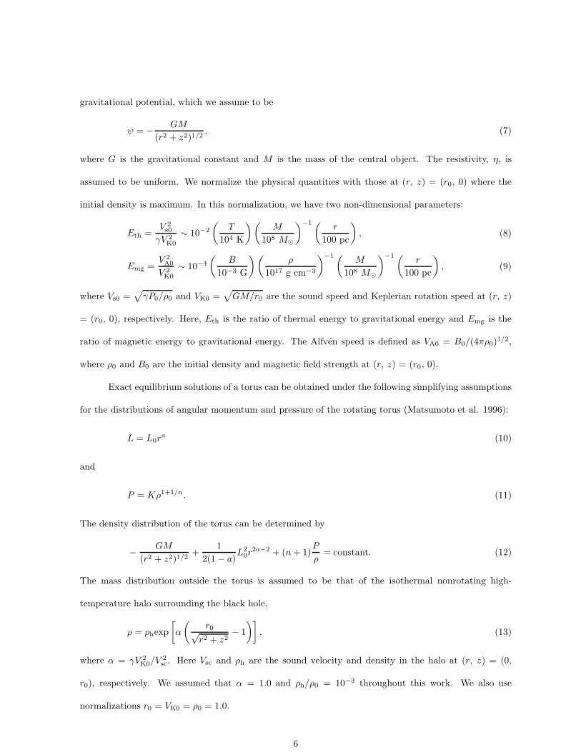
gravitational potential, which we assume to be

ψ = − GM

(r2 + z2)1/2, (7)

where G is the gravitational constant and M is the mass of the central object. The resistivity, η, is

assumed to be uniform. We normalize the physical quantities with those at (r, z) = (r0, 0) where the

initial density is maximum. In this normalization, we have two non-dimensional parameters:

Eth =V 2

s0

γV 2K0

∼ 10−2

(

T

104 K

)(

M

108 M

)−1(r

100 pc

)

, (8)

Emg =V 2

A0

V 2K0

∼ 10−4

(

B

10−3 G

)(

ρ

1017 g cm−3

)−1(M

108 M

)−1(r

100 pc

)

, (9)

where Vs0 =√

γP0/ρ0 and VK0 =√

GM/r0 are the sound speed and Keplerian rotation speed at (r, z)

= (r0, 0), respectively. Here, Eth is the ratio of thermal energy to gravitational energy and Emg is the

ratio of magnetic energy to gravitational energy. The Alfven speed is defined as VA0 = B0/(4πρ0)1/2,

where ρ0 and B0 are the initial density and magnetic field strength at (r, z) = (r0, 0).

Exact equilibrium solutions of a torus can be obtained under the following simplifying assumptions

for the distributions of angular momentum and pressure of the rotating torus (Matsumoto et al. 1996):

L = L0ra (10)

and

P = Kρ1+1/n. (11)

The density distribution of the torus can be determined by

− GM

(r2 + z2)1/2+

1

2(1 − a)L2

0r2a−2 + (n+ 1)

P

ρ= constant. (12)

The mass distribution outside the torus is assumed to be that of the isothermal nonrotating high-

temperature halo surrounding the black hole,

ρ = ρhexp

[

α

(

r0√r2 + z2

− 1

)]

, (13)

where α = γV 2K0/V

2sc. Here Vsc and ρh are the sound velocity and density in the halo at (r, z) = (0,

r0), respectively. We assumed that α = 1.0 and ρh/ρ0 = 10−3 throughout this work. We also use

normalizations r0 = VK0 = ρ0 = 1.0.

6

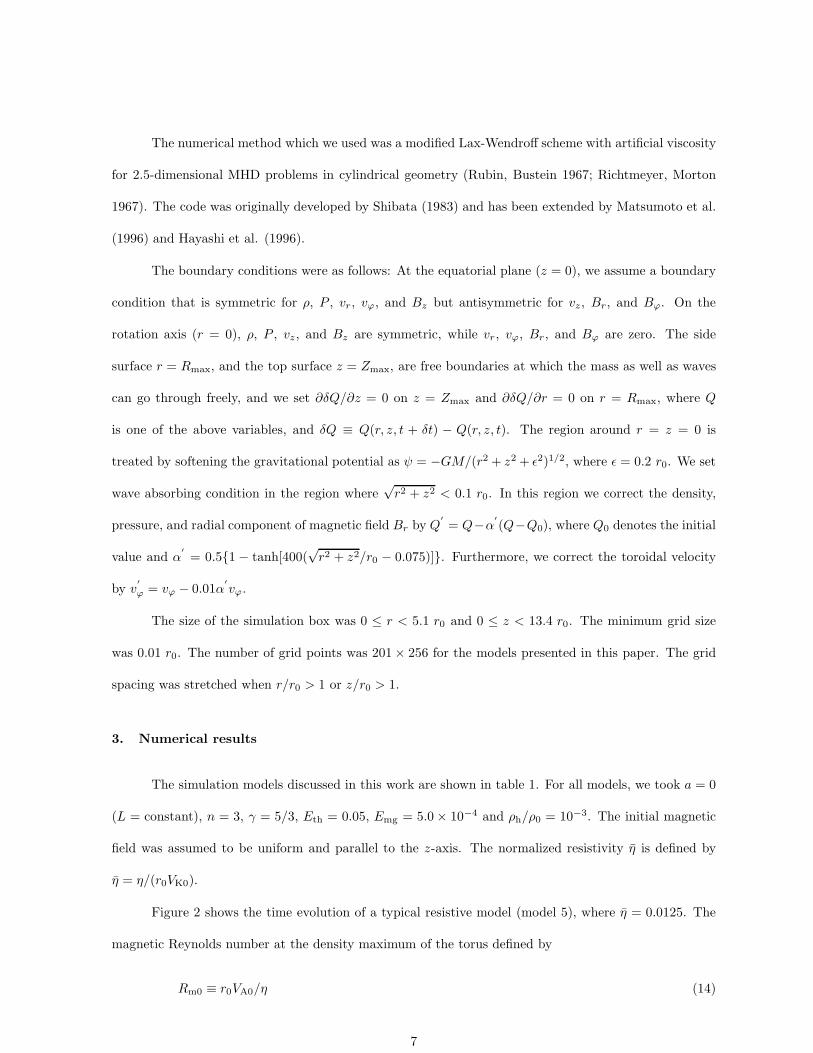
The numerical method which we used was a modified Lax-Wendroff scheme with artificial viscosity

for 2.5-dimensional MHD problems in cylindrical geometry (Rubin, Bustein 1967; Richtmeyer, Morton

1967). The code was originally developed by Shibata (1983) and has been extended by Matsumoto et al.

(1996) and Hayashi et al. (1996).

The boundary conditions were as follows: At the equatorial plane (z = 0), we assume a boundary

condition that is symmetric for ρ, P , vr, vϕ, and Bz but antisymmetric for vz, Br, and Bϕ. On the

rotation axis (r = 0), ρ, P , vz, and Bz are symmetric, while vr, vϕ, Br, and Bϕ are zero. The side

surface r = Rmax, and the top surface z = Zmax, are free boundaries at which the mass as well as waves

can go through freely, and we set ∂δQ/∂z = 0 on z = Zmax and ∂δQ/∂r = 0 on r = Rmax, where Q

is one of the above variables, and δQ ≡ Q(r, z, t + δt) − Q(r, z, t). The region around r = z = 0 is

treated by softening the gravitational potential as ψ = −GM/(r2 + z2 + ε2)1/2, where ε = 0.2 r0. We set

wave absorbing condition in the region where√r2 + z2 < 0.1 r0. In this region we correct the density,

pressure, and radial component of magnetic field Br by Q′

= Q−α′

(Q−Q0), where Q0 denotes the initial

value and α′

= 0.51 − tanh[400(√r2 + z2/r0 − 0.075)]. Furthermore, we correct the toroidal velocity

by v′

ϕ = vϕ − 0.01α′

vϕ.

The size of the simulation box was 0 ≤ r < 5.1 r0 and 0 ≤ z < 13.4 r0. The minimum grid size

was 0.01 r0. The number of grid points was 201× 256 for the models presented in this paper. The grid

spacing was stretched when r/r0 > 1 or z/r0 > 1.

3. Numerical results

The simulation models discussed in this work are shown in table 1. For all models, we took a = 0

(L = constant), n = 3, γ = 5/3, Eth = 0.05, Emg = 5.0 × 10−4 and ρh/ρ0 = 10−3. The initial magnetic

field was assumed to be uniform and parallel to the z-axis. The normalized resistivity η is defined by

η = η/(r0VK0).

Figure 2 shows the time evolution of a typical resistive model (model 5), where η = 0.0125. The

magnetic Reynolds number at the density maximum of the torus defined by

Rm0 ≡ r0VA0/η (14)

7

is Rm0 = 1.8. The magnetic Reynolds number near the surface of the torus is

Rmh ' r0VAh/η = r0(VA0/η)(VAh/VA0) = r0(VA0/η)(ρ0/ρh)1/2 ∼ 57. (15)

Here, VAh is the Alfven speed at (r, z) = (1.0, 0.75). The poloidal magnetic field lines depicted by

integrating the equation of magnetic lines of force (bottom panels) show that the surface layer of the

torus falls faster than the equatorial plane due to magnetic braking. For comparison, we show in figure

3 the results of non-resistive model (model 1). The bottom panels show the isocontours of rAϕ (Aϕ is

the vector potential) which depict poloidal magnetic field lines when η = 0. After one rotation period

(t = 2π), the magnetic field lines near the surface are already convected to the central gravitating object

in the non-resistive model (figure 3). In the resistive model (figure 2), however, this surface avalanche

(Matsumoto et al. 1996) is not so evident as that in non-resistive model; the magnetic field lines are only

slightly deformed.

The speed of the jet in the early stage (t < 9) of the resistive model is slower than that in the

non-resistive model. However, as the magnetic field lines are deformed and the angle from the equatorial

plane decreases (t = 18.5), the jet speed increases and approaches the Keplerian rotation speed of the

torus.

In the non-resistive model (figure 3), the jet-forming surface area of the torus is narrower than

that of the resistive model because some part of the surface layer moves outward by gaining angular

momentum, thus preventing the infall of the outer disk material. Inside the torus, strong twists are

accumulated, as shown in the isocontours of Bϕ in both the non-resistive model and the resistive model.

The torus expands in the vertical direction due to magnetic pressure produced by the accumulated toroidal

magnetic fields.

In the resistive model (figure 2), the magnetic field lines inside the torus approach straight lines

(see the bottom panels of figure 2). The torus is deformed into a disk-like shape and accretion proceeds

inside the torus by magnetically losing angular momentum. Figure 4 shows the numerical results for a

highly resistive model (model 7; η = 0.05, Rm0 = 0.4, Rmh ∼ 13). In this model, since Rm0 < 1, the

torus is stable for the magnetorotational instability (Sano et al. 1998). These results indicate that the

magnetic field lines are deformed only slightly and that magnetic twists are not accumulated inside the

8

torus. Only weak outflow with velocity v ∼ 0.2VK0 appears in this model.

Figure 5–7 show 3D pictures of the magnetic field lines and isosurface of density for models 5,

1, and 7, respectively. As the resistivity increases, the angle which the large-scale magnetic field lines

make with the vertical axis decreases. The magnetic twist also decreases with the resistivity. The density

isosurfaces evidently show that bipolar outflow is produced in model 5 and model 1.

Figure 8 shows the time variation of the temperature distribution (gray scale) and rAϕ (Aϕ is

vector potential), which depicts magnetic field lines and velocity vectors for models 5, 1, and 7. Figure

8a (upper three panels) is for model 5. In this mildly diffusive model, mass accretion and mass outflow

take place continuously. Figure 8b (middle three panels) is for model 1. In this non-diffusive model, the

mass accretion and mass outflow take place episodically. At t = 5.96, the first avalanching mass accretion

and mass outflow take place. Subsequently, the accretion rate decreases because some parts of the disk

material obtain angular momentum and prevent the outer region from infalling. Around t = 15.9, surface

mass accretion occurs again. Figure 8c (bottom three panels) is for model 7. Almost no mass accretion

and mass outflow take place.

Figures 9a and b show the mass outflow rate for various models. The mass outflow rate is defined

as

Mjet = 2 ×∫ 3.0

0

2πrρVzdr (16)

at z = 3.1 r0. When η ∼ 0.0125, it increases monotonically with time and approaches a quasi-steady

value (model 5, model 6). When η < 0.0125, however, the mass outflow rate has several peaks (model 1,

model 2, model 3, model 4). In these models jet production takes place episodically. When η > 0.0125

(model 7) the mass outflow rate approaches zero. Figures 10a and b show the time variation of the mass

accretion rate, defined as

Macc = 2 ×∫ 0.4

0

2πrρvrdz (17)

at r = 0.3 r0. When η takes a value between 0 and 0.01, the time averaged-accretion rate when t 0

takes almost the same value independent of η, although the accretion rate increases more rapidly with

time when η ∼ 0. When 0.01 < η < 0.05, the accretion rate approaches a quasi-steady value, but the

9

peak accretion rate is smaller than in models with η < 0.01. When η ≥ 0.05, almost no accretion takes

place.

The numerical results indicate the existence of three-regimes of jet formation and accretion de-

pending on the resistivity, (1) episodic jet formation and accretion for small resistivity: (Rm0 > 2.0), (2)

quasi-steady jet formation and accretion for mildly-resistive (1 < Rm0 < 2.0) disk and (3) almost no jet

formation and no accretion in highly resistive models (Rm0 < 1). In highly resistive models, since the

torus medium almost slips the magnetic field lines by magnetic diffusion, magnetic braking is insufficient

to induce accretion.

Figure 11 shows isocontours of the magnetic Reynolds number log10Rm = log10(VAλ0/η). Here, λ0

is a characteristic scale of the magnetorotational instability at t = 0 at (r, z) = (r0, 0), which is defined

as λ0 = 2πVA0/Ω0, where VA0 and Ω0 are the Alfven speed and the rotation angular speed at (r, z) = (r0,

0), respectively. In figure 11, the solid curves show the region where diffusion is not effective (Rm > 1)

and the dotted curves show the region where diffusion is effective (Rm < 1). In figure 11a, the diffusive

region occupies about half the volume in the torus. In this model, diffusion does not have much affection

on the disk surface where a jet is formed. No diffusive region appears in figure 11b because model 1 is a

non-diffusive model. Figure 11c shows a highly diffusive model. Since the diffusive region occupies almost

the total area in the torus, magnetic braking is suppressed and the accretion is not sufficient to form a

jet. To illustrate the twist level of the magnetic field lines, we show in figure 12 the time variation of the

ratio of the toroidal magnetic field, Bϕ, to the poloidal magnetic field, Bp, along a field line determined

by integrating the equation of the magnetic lines of force inward from (r, z) = (1.0, 3.1). Figure 12

illustrates that the resistive model [model 5; figure 12a, model 7; figure 12c] shows smaller twists than

that in non-diffusive model [model 1; figure 12b]. In the non-diffusive model, a strong twist appears at

t = 5.5 and propagates outward when the jet is created. Figure 12c illustrates a highly resistive model

(model 7) which hardly shows outflows and has the smallest toroidal magnetic field component.

Figure 13 shows the poloidal velocity, the poloidal fast velocity, poloidal Alfven velocity, and

poloidal slow velocity along a magnetic field line. In model 5 and model 1, snapshots were taken at the

start time of jet formation. In model 7, the velocities were measured at t ∼ 8π. Figure 13a (top panels)

10

is for model 5 (η = 1.25 × 10−2). In model 5, the jet is accelerated faster than both the Alfven velocity

and the slow velocity and its speed becomes about the Keplerian speed. Figure 13b (middle panels) is for

model 1 (η = 0). The jet is accelerated similarly to model 5 and the maximum poloidal speed becomes

about 1.4 times the Keplerian speed. Figure 13c (bottom two panels) is for model 7 (η = 5.0× 10−2). A

jet is not formed and the poloidal velocity does not exceed either the slow velocity or the Alfven velocity.

4. Discussion

4.1. Dependence of the Numerical Results on the Diffusivity

We have studied the effects of resistivity on the magnetically driven accretion and jet formation

from a torus threaded by large-scale poloidal magnetic fields. When η ∼ 0, the surface layer of the

torus infalls faster than the equatorial region, like an avalanche, due to magnetic braking. As the angle

between the deformed magnetic field lines and the vertical direction increases, a magnetically driven jet

appears. The jet formation and mass accretion occur episodically. This episodic accretion takes place

because parts of the torus matter move radially outward by gaining angular momentum and hinder the

mass outside of it to accrete. The magnetorotational instability developing inside the torus also helps to

generate the episodic behavior. The speed of the jet nearly equals the Keplerian rotation speed. When

0.0067 < η < 0.0125, the torus approaches a quasi-steady state without showing episodic accretion. When

0.0125 < η < 0.05, mass accretion and jet formation take place, but the mass accretion rate and mass

outflow rate decrease with η. When η > 0.05, neither mass accretion nor jet formation takes place.

4.2. Evaluation of Turbulent Diffusivity

In this paper, we carried out 2.5-dimensional simulations by explicitly including uniform magnetic

diffusivity. Even when the classical Spitzer-type resistivity is small, turbulent diffusivity can be gener-

ated by three-dimensional effects. In three dimensions, non-axisymmetric instabilities generate magnetic

turbulence (Hawley et al. 1995; Matsumoto, Tajima 1995; Brandenburg et al. 1995). The turbulence in

accretion disks generates effective magnetic diffusion. Here, let us estimate the effective diffusivity in an

accretion disk based on a marginal stability analysis (Matsumoto, Tajima 1995). The marginal stability

11

model belongs to a self-organized criticality (SOC) model (e.g., Bak et al. 1988; Mineshige et al. 1994) in

complex systems, which claims that the system spontaneously evolves to a critical state between unstable

states and stable states. We can obtain a marginally stable state by equating the growth rate of the

magnetorotational instability, γBH, and the stabilization rate due to magnetic diffusivity, ηtk2, where ηt

is the turbulent diffusion coefficient and k = 2π/λmax, here, λmax is the most unstable wavelength, which

we take λmax = 2πVA/ΩK0. In the marginally stable state, γBH = ηtk2. Since the growth rate of the

magnetorotational instability is on the order of γBH ∼ ΩK0,

VK0r0ηt

∼ VK0r0ΩK0/k2

∼ (2π)2VK0r0ΩK0λ2

max

∼ V 2K0

V 2A

∼ β

2E−1

th , (18)

where β = Pgas/Pmag. Since β ' 10 in the nonlinear saturated stage of the magnetorotational instability

(Stone et al. 1996; Matsumoto 1999) and Eth = 0.05 in our model torus, we obtain ηt/(VK0r0) ∼ 0.01.

From this result, the effective diffusivity in the marginally stable state of the accretion disk can be

estimated as η = η/(VK0r0) ∼ 0.01.

We have shown that the numerical results of resistive MHD simulations sensitively depend on η

when η ∼ 0.01. The order of magnitude estimates of the turbulent resistivity, ηt presented here are

not sufficient to determine the dependence of the turbulent resistivity on the disk parameters (e.g., disk

thickness). To obtain exact values of ηt, we need to carry out global 3D MHD simulations. Hawley

(2000) and Machida et al. (2000) published the results of 3D global MHD simulations stating from a

geometrically thick disk. Much higher resolution simulations are necessary to show the difference of ηt for

different disk types. Such simulations are now in progress and will be reported in our subsequent papers.

In this work, we assumed uniform resistivity which mimics the turbulent diffusion in accretion disks.

A rather different model for dissipation is magnetic reconnection in a hot corona. By assuming anomalous

resistivity, Hayashi et al. (1996) carried out resistive MHD simulations of magnetic reconnection in

magnetic loops connecting the central star and surrounding accretion disk. They successfully reproduced

the formation of bipolar plasma outflows and X-ray flares. Magnetic reconnection of magnetic loops

whose footpoints are both on accretion disks have been simulated by Romanova et al. (1998). The

coronal activities of accretion disks acompanying magnetic reconnection are more complicated processes

12

which cannot be mimiced by uniform resistivity, and is thus beyond the scope of this paper.

4.3. Application to AGN Molecular Torus

Next, we discuss the application of these numerical results to AGNs. Observations indicate that

molecular gas whose mass is 1010 M exists in the central region of high-luminosity IRAS galaxies (Scoville

et al. 1991) and that a circumnuclear starburst torus whose radius is between several tens pc and 1 kpc

exists in the central region of Seyfert galaxies (Wilson et al. 1991, Forbes et al. 1994, Storchi-Bergmann

et al. 1996). The ionization rate of the torus may be low because the torus exists far from the central

black hole. We should discuss whether magnetic braking is effective in a low-ionized gas torus. The

magnetic diffusivity in partially ionized gas is

η = 6.5 × 1012(lnΛ)T−3/2

(

1 +τeiτen

)

cm2 s−1 (19)

and

τeiτen

= 1.3 × 10−5 1

χ

(

T

500 K

)21

ln Λ(20)

(Spitzer 1962). Here, τei, τen, χ, and ln Λ are the electron–ion collision time, electron–neutral atom

collision time, ionization rate, and Coulomb logarithm (∼ 10), respectively. When the number density of

gas satisfies n 1,

η ' 8 × 103

(

T

500 K

)1/21

χ(21)

(Gammie 1996), where the ionization rate, χ, is

χ =

10−5n−1/2 104 < n < 1010

n−1 1010 < n

(22)

(Norman, Heyvaerts 1985). Assuming that a gas torus exists at 100 pc from the central black hole and

that the temperature of the torus is 100 K, the magnetic Reynolds number is

Rm ∼ vAH

η∼ 1014

( vA1 km s−1

)

(

H

10 pc

)

×(

T

100 K

)−1/2( n

104 cm−3

)−1/2

. (23)

13

Here, H is the thickness of the gas torus. Since Rm 1, magnetic braking is effective for charged

particles. We should discuss whether magnetic braking is effective for neutral particles, too. The velocity

of a neutral particle is influenced by ambipolar diffusion. The velocity difference, vd, between charged

particles and neutral particles is

vd ∼ 104( n

104 cm3

)−2 ( χ

10−7

)−1

×(

B

50 µG

)2(H

10 pc

)−1

cm s−1 (24)

(Tajima, Shibata 1997). Since the velocity difference, vd ∼ 104 cm s−1, is smaller than the dynamical

velocity, vdyna ∼ 107 cm s−1, neutral particles also fall to the black hole when magnetic braking takes

place around the surface of the torus. We conclude that magnetic braking can be effective in an AGN

gas torus. Recently, Hawley and Stone (1998) carried out 3D MHD simulations of an ion–neutral fluid.

We would like to confirm the above discussion in the near future by extending our MHD code to an

ion–neutral MHD code.

Tables 2 and 3 show the mean and maximum mass outflow rates and accretion rates when we

apply our numerical results to AGNs which have MBH = MBH9 = 109 M and circumnuclear gas torus

with mass Mtorus = M8 = 108 M. In order to explain the energy release rate of quasars,

L = εMc2 ∼ 3 × 1045( ε

0.05

)

(

M

1 M yr−1

)

erg s−1. (25)

where ε is the conversion efficiency of mass energy, we need a mass accretion rate of at least 1 M yr−1.

Table 3 shows that when η < 0.05 VK0r0 in an AGN gas torus, we can explain quasar activity.

4.4. Order-of-Magnitude Estimation of the Mass Accretion Rate

We can estimate the mass accretion rate by approximating the torus by a rectangular box with

height r0. The diffusion region of the torus is approximated by a rectangular box with height λ, as shown

in figure 14. The disk gas couples with the magnetic field in a surface region with thickness r0 − λ. The

accretion rate is

Macc = 4π

∫

ρVaccrdz ∼ 4π × 0.1ρ0r20Vacc

(

1 − λ

r0

)

∼ 0.25ρ0r30ΩK0

(

1 − λ

r0

)

, (26)

14

where

Vacc ∼ 0.1r0ΩK0. (27)

Here, the density of the torus is assumed to be constant, ρ = 0.25ρ0. The size of λ is determined by the

condition that the magnetic Reynolds number, Rm, is unity, Rm = λVA0/η ∼ 1. Thus,

λ ∼ ηRm

VA0

∼ η

VA0

. (28)

Using equations (26), (27), and (28), the normalized magnetic diffusivity, η ≡ η/(r0VK0), and Emg =

(VA0/VK0)2 [equation (9)], we can obtain a normalized mass accretion rate

Macc

ρ0r20VK0

∼ 0.25(

1 − E−1/2mg η

)

. (29)

This equation can explain the numerically obtained mass accretion rate when 0 < η < 1.4 × 10−2, but

can not explain the accretion rate when η > 5.0 × 10−2 (see figure 15). To improve this point, we take

into consideration the density gradient. The mass accretion rate is

M ∼∫ r0

λ

4πr0ρ(z)dzVacc ∼ 4πr0ρsurfaceHVacc (for λ r0)

∼ 10r20ρ0 exp

[

−1

2

(

λ

H

)2]

H × 0.1ΩK0

∼ r20ρ0 exp

[

−1

2

(

ηΩK0

VA0Vs0

)2]

Vs0

∼ ρ0r20Vs0 exp

[

−1

2

(

ηr20Ω2K0

VA0Vs0

)2]

∼ ρ0r20Vs0 exp

[

−1

2

(

ηE−1/2mg E

−1/2

th

)2]

. (30)

Here, E1/2

th = Vs0/VK0. From equation (30), normalized mass accretion rate becomes

M

ρ0r20VK0

∼ E1/2

th exp[−1

2

(

ηE−1/2mg E

−1/2

th

)2

]. (31)

Here, H is the scale height,

H

r0∼ Vs0

VK0

∼ Vs0

r0ΩK0

.

Figure 15 shows the normalized mass accretion rate given by equations (29), (31), and the numerical

result. From this figure, the mass accretion rate estimated by equation (31) can better fit the results of

numerical simulations.

15

4.5. Concluding Remarks

In this paper, we have presented the results of 2.5-dimensional simulations of a magnetized torus

by explicitly including magnetic diffusivity. When we carry out three-dimensional simulation, the effects

of turbulent magnetic diffusion automatically comes in when the torus becomes turbulent. We would

like to extend our model to 3D in the near future. Furthermore, when we apply the results to AGNs,

self-gravitational effects may be important when the torus mass is as large as Mtorus ∼ 108 M. We

would like to discuss the effects of self-gravity in forthcoming papers.

The numerical computations were carried out on VX/4R at the Astronomical Data Analysis Center

of the National Astronomical Observatory, Japan. This work is supported in part by the grant for

special field of Ministry of Education, Sports and Culture (10147105) and Japan Science and Technology

Coorporation (ACT-JST).

16

Reference

Bak P., Tang C., Wiesenfeld K. 1988, Phys. Rev. Lett. A38, 364

Balbus S.A., Hawley J.F. 1991, ApJ 376, 214

Blandford R.D., Payne D.G. 1982, MNRAS 199, 883

Brandenburg A., Nordlund A., Stein R.F., Torkelsson U. 1995, ApJ 446, 741

Forbes D.A., Norris R.P., Williger G.M., Smith R.C. 1994, AJ 107, 984

Gammie C.F. 1996, ApJ 457, 355

Goodson A.P., Bohm K.-H., Winglee R.M. 1999, ApJ 524, 142

Goodson A.P., Winglee R.M., Bohm K.-H. 1997, ApJ 489, 199

Grosso N., Montmerle T., Feigelson E.D., Andre P., Casanova S., Gregorio-Hetem J. 1997, Nature 387,

56

Hawley J.F. 2000, ApJ 528, 462

Hawley J.F., Balbus S.A. 1992, ApJ 400, 595

Hawley J.F., Gammie C.F., Balbus S.A. 1995, ApJ 440, 742

Hawley J.F., Stone J.M. 1998, ApJ 501, 758

Hayashi M.R., Shibata K., Matsumoto R. 1996, ApJ 468, L37

Hirose S., Uchida Y., Shibata K., Matsumoto R. 1997, PASJ 49, 193

Jaffe W., Ford H., Ferrarese L., van den Bosch, F., O’Connell R.W. 1996, ApJ 460, 214

Kaburaki O. 1987, MNRAS 229, 165

Koyama K., Hamaguchi K., Ueno S., Kobayashi N., Feigelson E.D. 1996, PASJ 48, L87

Kudoh T., Matsumoto R., Shibata K. 1998, ApJ 508, 186

Kudoh T., Shibata K. 1997, ApJ 474, 362

Lovelace R. V. E., Mehanian C., Mobarry C. M., Sulkanen M. E. 1986, ApJS 62, 1

Lubow S.H., Papaloizou J.C.B., Pringle J.E. 1994, MNRAS 268, 1010

Machida M., Hayashi M.R., Matsumoto R. 2000, ApJ 532, L67

Matsumoto R. 1999, Numerical Astrophysics, eds S.M. Miyama, K. Tomisaka, T. Hanawa (Kluwer Aca-

demic Publishers, Dordrecht), p195

17

Matsumoto R., Shibata K. 1997, Accretion Phenomena and Related Outflows, IAU Colloquium 163, ASP

Conference Series Vol. 121, ed D.T. Wickramasinghe, G.V. Bicknell, L. Ferrario, p443

Matsumoto R., Tajima T. 1995, ApJ 445, 767

Matsumoto R., Uchida Y., Hirose S., Shibata K., Hayashi M.R., Ferrari A., Bodo G., Norman C. 1996,

ApJ 461, 115

Meier D.L., Edgington S., Godon P., Payne D.G., Lind K.R. 1997, Nature 388, 350

Miller K.A., Stone J.M. 1997, ApJ 489, 890

Mineshige S., Ouchi N. B., Nishimori H. 1994, PASJ 46, 97

Norman C., Heyvaerts J. 1985, A&A 147, 247

Ogilvie G.I. 1997, MNRAS 288, 63

Ouyed R., Pudritz R.E., Stone J.M. 1997, Nature 385, 409

Pudritz R. E., Norman C. A. 1983, ApJ 274, 677

Richtmeyer R.D., Morton K.W. 1967, Difference Methods for Initial-Value Problems, 2nd ed (Interscience

Publishers, New York) ch13

Romanova M.M., Ustyugova G.V., Koldoba A.V., Chechetkin V.M., Lovelace R.V.E. 1998, ApJ 500, 703

Rubin E.L., Burnstein S.Z. 1967, J. Comp. Phys. 2, 178

Sano T., Inutsuka S., Miyama S.M. 1998, ApJ 506, L57

Scoville N.Z., Sargent A.I., Sanders D.B., Soifer B.T. 1991, ApJ 366, L5

Shibata K. 1983, PASJ 35, 263

Shibata K., Uchida Y. 1986, PASJ 38, 631

Shu F., Najita J., Ostriker E., Wilkin F., Ruden S., Lizano S. 1994a, ApJ 429, 781

Shu F.H., Najita J., Ruden S. P., Lizano S. 1994b, ApJ 429, 797

Spitzer L.Jr 1962, Physics of Fully Ionized Gases (Interscience Publishers, New York), p133

Stone J.M., Hawley J.F., Gammie C.F., Balbus S.A. 1996, ApJ 463, 656

Stone J.M., Norman M.L. 1992, ApJS 80, 753

Stone J.M., Norman M.L. 1994, ApJ 433, 746

Storchi-Bergmann T., Wilson A.S., Baldwin J.A. 1996, ApJ 460, 252

18

Tajima T., Shibata K. 1997, Plasma astrophysics (Addison-Wesley, Reading, Massachusetts)

Uchida Y., Shibata K. 1985, PASJ 37, 515

Ustyugova G.V., Koldoba A.V., Romanova M.M., Chechetkin V.M., Lovelace R.V.E. 1995, ApJ 439, L39

Wilson A.S., Helfer T.T., Haniff C.A., Ward M.J. 1991, ApJ 381, 79

Yabe T., Aoki T. 1991, Comp. Phys. Comm. 66, 219

19

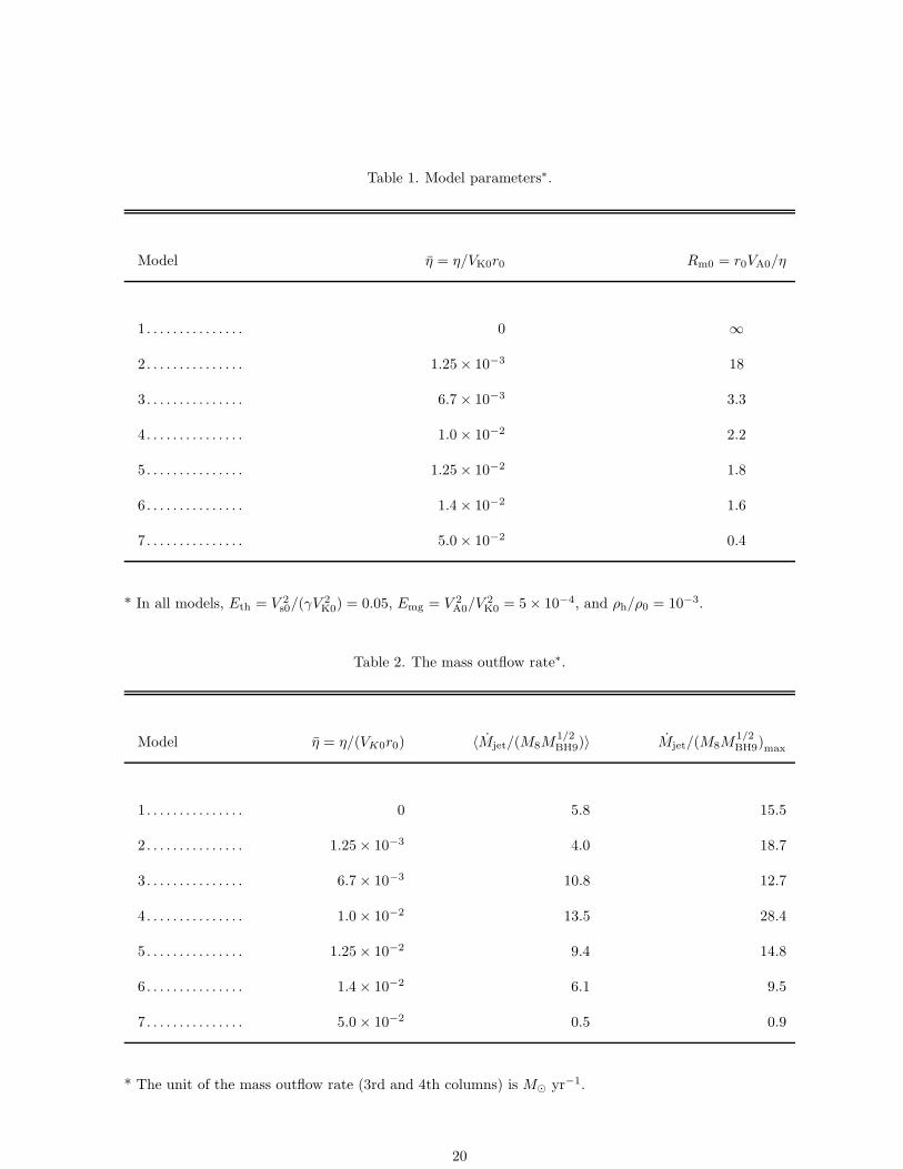
Table 1. Model parameters∗.

Model η = η/VK0r0 Rm0 = r0VA0/η

1 . . . . . . . . . . . . . . . 0 ∞

2 . . . . . . . . . . . . . . . 1.25 × 10−3 18

3 . . . . . . . . . . . . . . . 6.7 × 10−3 3.3

4 . . . . . . . . . . . . . . . 1.0 × 10−2 2.2

5 . . . . . . . . . . . . . . . 1.25 × 10−2 1.8

6 . . . . . . . . . . . . . . . 1.4 × 10−2 1.6

7 . . . . . . . . . . . . . . . 5.0 × 10−2 0.4

* In all models, Eth = V 2s0/(γV

2K0) = 0.05, Emg = V 2

A0/V2K0 = 5 × 10−4, and ρh/ρ0 = 10−3.

Table 2. The mass outflow rate∗.

Model η = η/(VK0r0) 〈Mjet/(M8M1/2

BH9)〉 Mjet/(M8M1/2

BH9)max

1 . . . . . . . . . . . . . . . 0 5.8 15.5

2 . . . . . . . . . . . . . . . 1.25 × 10−3 4.0 18.7

3 . . . . . . . . . . . . . . . 6.7 × 10−3 10.8 12.7

4 . . . . . . . . . . . . . . . 1.0 × 10−2 13.5 28.4

5 . . . . . . . . . . . . . . . 1.25 × 10−2 9.4 14.8

6 . . . . . . . . . . . . . . . 1.4 × 10−2 6.1 9.5

7 . . . . . . . . . . . . . . . 5.0 × 10−2 0.5 0.9

* The unit of the mass outflow rate (3rd and 4th columns) is M yr−1.

20

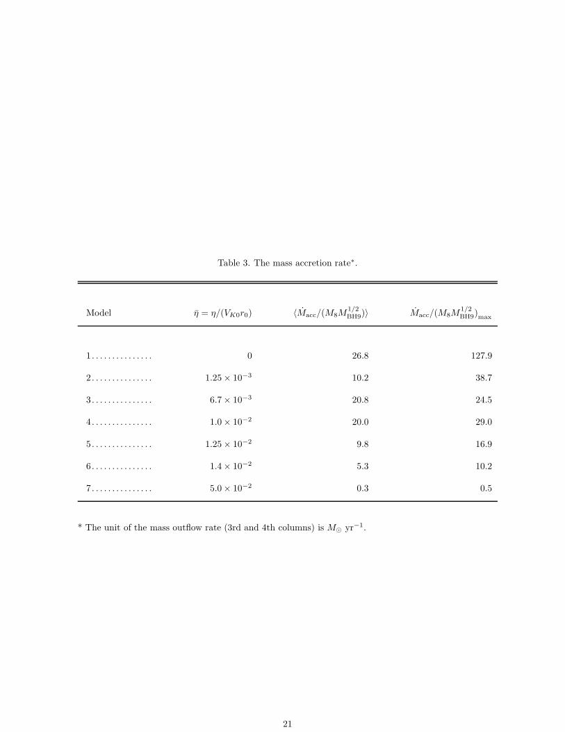
Table 3. The mass accretion rate∗.

Model η = η/(VK0r0) 〈Macc/(M8M1/2

BH9)〉 Macc/(M8M1/2

BH9)max

1 . . . . . . . . . . . . . . . 0 26.8 127.9

2 . . . . . . . . . . . . . . . 1.25 × 10−3 10.2 38.7

3 . . . . . . . . . . . . . . . 6.7 × 10−3 20.8 24.5

4 . . . . . . . . . . . . . . . 1.0 × 10−2 20.0 29.0

5 . . . . . . . . . . . . . . . 1.25 × 10−2 9.8 16.9

6 . . . . . . . . . . . . . . . 1.4 × 10−2 5.3 10.2

7 . . . . . . . . . . . . . . . 5.0 × 10−2 0.3 0.5

* The unit of the mass outflow rate (3rd and 4th columns) is M yr−1.

21

Figure Captions

Fig. 1. Schematic picture of the simulation model and simulation box. A differentially rotating gas torus is

threaded by global magnetic fields. Numerical simulations were carried out by using an axisymmetric

MHD code in cylindrical coordinates.

Fig. 2. Time variation of ρ (the contour step width is 0.3 in logarithmic scale of ρ), poloidal velocity

vectors v, isocontours of toroidal magnetic field component Bϕ (the contour step width is 0.1), poloidal

magnetic field lines Bp in model 5 (η = 1.25×10−2). The surface layer of the torus falls to the central

object because of magnetic braking. A bipolar jet is formed along the large-scale poloidal magnetic

field lines (see velocity vectors v).

Fig. 3. Time variation of ρ (the contour step is 0.3 in logarithmic scale), poloidal velocity vectors v,

isocontours of toroidal magnetic field component Bϕ (the contour step is 0.1), poloidal magnetic field

lines Bp in model 1 (η = 0). The magnetic braking is more effective than in model 5 (see Bp). The

magnetic twist is lager than in model 5 (see contours of Bϕ) and the jet width is smaller than in model

5 (see v).

Fig. 4. Time variation of ρ (the contour step is 0.3 in logarithmic scale), poloidal velocity vectors v,

isocontours of toroidal magnetic field component Bϕ (the contour step is 0.1), poloidal magnetic field

lines Bp in model 7 (η = 5.0 × 10−2). The magnetic braking is not effective and mass accretion does

not take place. The magnetic twist is hardly accumulated and a jet is not formed.

Fig. 5. 3D images of the time variation of numerical results for model 5 (η = 1.25 × 10−2). The top

panels show the isosurface of the density and the magnetic field lines. The middle panels show the

time variation of the two magnetic field lines viewed from the side. The bottom panels show the time

variation of two magnetic field lines seen from the top.

Fig. 6. 3D images of the time variation of model 1 (η = 0). The top panels show the isosurface of the

density and the magnetic field lines. The middle panels show the time variation of two magnetic field

lines seen from the side. The bottom panels show the time variation of two magnetic field lines seen

from the top.

22

Fig. 7. 3D images of the time variation of model 7 (η = 5.0× 10−2). The top panels show the isocontour

of the density and the magnetic field lines. THe middle panels show the time variation of two magnetic

field lines viewed from the side. The bottom panels show the time variation of two magnetic field lines

seen from the top.

Fig. 8. Time variation of the temperature distribution (gray scale) and rAϕ (Aϕ is the vector potential),

which approximately depicts the magnetic field lines and the velocity vectors. The top panels are for

model 5. The middle panels are for model 1. The bottom panels are for model 7.

Fig. 9. Time variation of the mass outflow rate defined as Mjet = 2∫ 3.0

02πrρVzdr at z = 3.1 for all

models. As η increases (from model 1 to model 6), the outflow changes its character from episodic

outflow to qusi-steady outflow. In a highly diffusive model (model 7), mass outflow hardly takes place.

Fig. 10. Time variation of the mass accretion rate, defined as Macc = 2∫ 0.4

02πrρVrdz at r = 0.3 of all

models. As η becomes larger (from model 1 to model 6), the mass accretion changes from episodic

accretion to quasi-steady accretion. In model 7, mass accretion hardly takes place.

Fig. 11. Isocontours of magnetic Reynolds number (Rm = 2πVAVA0/ηΩ0) at the initial state (t = 0) and

at about 2.5 rotation time (t = 16.4). (a) model 5 (η = 1.25 × 10−2), (b) model 1 (η = 0), and (c)

model 7 (η = 5.0 × 10−2). The region depicted by solid curves shows where diffusion is not effective

(Rm > 1), and the region depicted by dotted curves correspond to the diffusive region (Rm < 1). In

a mildly diffusive model (model 5), the diffusive region occupies about half the area in the torus. In

the non-diffusive model (model 1), no diffusive region appears. In a highly diffusive model (model 7),

almost the total region of the torus is diffusive.

Fig. 12. Ratio of | Bϕ | to | Bp | along B in (a) model 5 (η = 1.25 × 10−2), (b) model 1 (η = 0), and

(c) model 7 (η = 5.0 × 10−2). In the diffusive model 5 (η = 1.25 × 10−2), the twist of magnetic field

accumulates gradually. In non-diffusive model 1, magnetic field lines are twisted in short time, and we

can see that a strong twist propagates along the magnetic field line. In model 7, the twist of magnetic

field slowly accumulates, but takes long time. Mass outflow and mass accretion hardly occur in this

model.

23

Fig. 13. Poloidal velocity, poloidal fast velocity, poloidal Alfven velocity and poloidal slow velocity along

a magnetic field line for (a) model 5 (η = 1.25× 10−2, t = 16.2), (b) model 1 (η = 0, t = 5.8), and (c)

model 7 (η = 5.0 × 10−2, t = 27). The filled circles denote the slow point and the open circles show

the Alfven point nearest from the equatorial plane.

Fig. 14. Schematic picture of a torus modified to roughly estimate the mass accretion rate. We approxi-

mate the cross section of the torus by a square.

Fig. 15. Comparison between the numerically obtained mass accretion rate and analytically obtained

estimation of the mass accretion rate. The equation (31) gives a better fit than equation (29).

24

This figure "fig01.jpg" is available in "jpg" format from:

http://arXiv.org/ps/astro-ph/0011165












































Documents

arXiv:astro-ph/0011165 v1 8 Nov 2000 - core.ac.uk · Since the angular momentum of the torus is extracted due to magnetic braking, ... the system evolves ... in the center of a galaxy